Coupling vs decoupling approaches for PDE/ODEsystems modeling intercellular signaling

Thomas Carraro∗ Elfriede FriedmannDaniel Gerecht

Institute for Applied MathematicsHeidelberg University, Germany

August 31, 2018

Abstract

We consider PDE/ODE systems for the simulation of intercellular signal-ing in multicellular environments. The intracellular processes for each celldescribed here by ODEs determine the long-time dynamics, but the PDEpart dominates the solving effort. Thus, it is not clear if commonly useddecoupling methods can outperform a coupling approach. Based on a sen-sitivity analysis, we present a systematic comparison between coupling anddecoupling approaches for this class of problems and show numerical results.For biologically relevant configurations of the model, our quantitative studyshows that a coupling approach performs much better than a decoupling one.

keywords Coupled PDE/ODE systems, Sensitivity analysis, Multilevel precondi-tioner, Intercellular Signaling

1 Introduction

Cellular signaling has been mathematically described by a variety of models mostlyrelying on large systems of ordinary differential equations (ODE) [1]. These earliermodels were extended by partial differential equations (PDE) to accurately considerconcentration gradients and their effect [2, 3, 4, 5]. In our intercellular model weconsider the diffusion and action of small signaling proteins in the intercellular spacedescribed by PDE, i.e. reaction-diffusion equations, coupled on the cell surfaces withODEs responsible for the intracellular dynamics. This coupling of mixed differentialequations allows mainly two strategies for an implicit solver: (1) nonlinear methodsamong them the nonlinear multigrid method also called “full approximation scheme”(FAS) [6, 7], (2) linearization based approaches (Newton-type). These methods canbe used in a combined approach, where for example a Newton-type method canbe used as smoother for a FAS and a linear or a nonlinear multigrid can be used

∗thomas.carraro@iwr.uni-heidelberg.de

1

arX

iv:1

603.

0274

4v1

[m

ath.

NA

] 9

Mar

201

6

as a preconditioner for a Newton-type method. The comparison and discussion ofadvantages and disadvantages of these strategies that depend on many aspects like,e.g. the accuracy of the Jacobian approximation [8], is not the focus of our work.Moreover, since in the considered coupled PDE/ODE system the linearization is nota critical point we choose a Newton-type method preconditioned by a linear multigridand study the effect of splitting the linearization. A decoupling solution approach,based on a fixed-point method, is often used when restrictions on accuracy can berelaxed in order to allow an easier numerical treatment of complicated problems.Such an approach makes it possible to reuse existing solvers and is widely usedin numerical methods for coupled systems, see [9, 10, 11, 12, 13, 14]. In case ofstrongly coupled equations (see Section 4 for the definition of strong coupling usedhere), this strategy leads usually to high computational costs through very smalltime steps needed to reduce the strength of the coupling. In fact, the convergenceof the fixed-point iterations is typically linear with the convergence rate dependingon the used block-iterative method and on the strength of the coupling since itdepends on the spectral radius of the matrices involved [15]. Therefore a drawbackof decoupling solvers is their low convergence and possibly divergence. On thecontrary, the drawback of fully implicit solvers is mainly that they demand for theimplementation of a special-purpose code.

We consider PDE/ODE systems for the simulation of intercellular signaling inmulticellular environments. Since the ODE part does not lead to a large discretiza-tion system like the PDE part, it is not clear if a decoupling method can outperforma coupling approach. In fact other works with PDE/ODE models have used de-coupling approaches for systems arising in biological applications, e.g. blood flowincluding chemical interaction [16, 17], signal transduction [4], cardiovascular flow[9], cancer invasion [18]. With the exception of [9] these works do not consider a com-parison with a monolithic approach. In addition, for the most of these applicationsit is not clear whether the strength of the coupling is strong or weak.

In this context, the scope of our work is to present a systematic comparison be-tween coupling and decoupling approaches for this class of problems. The methodis based on a sensitivity analysis to compute the strength of the coupling. Addition-ally, we compare a multigrid method in which the coupling is considered only at thecoarsest level to a fully coupling approach. There are few works that deal with thefully coupling solution process of dimensionally heterogeneous systems such as [19].Furthermore, we focus on the solution of local microenvironments. Therefore, thissolution process can be used for example as local solver for nonlinear preconditionerof Newton-type methods [20] or domain decomposition methods [21].

Outline The paper is organized as follows. In Section 2 we give an abstract de-scription of the model. We present the mathematical formulation and the functionalsetting. We discretize the coupled PDE/ODE system by the finite element method(FEM) in Section 3. We use a sensitivity approach in Section 4 to analyze thecoupling of the PDE/ODE system and in Section 5 we present different solving ap-proaches for the coupled system. We present the numerical results exemplarily fora particular application and discuss numerical aspects in Section 6. In Section 7 wedescribe a realistic configuration and give a biological interpretation to the resultsobtained.

2

2 Mathematical Models for Intercellular Signal-

ing

Our intercellular signaling model consists of one PDE equation for the interactionbetween the cells in the intercellular area Ω ⊂ R3 coupled with ODEs for the intra-cellular processes. We denote by Nc the number of cells in Ω and indicate by Γithe boundary of each cell i for i = 1, . . . , Nc. The outer boundary of Ω is denotedby Γout, see Figure 1.

Figure 1: Visualization of the computational domain

Γout

Γi

(a) 8 interacting cells with surfacesΓi

(b) Intercellular area Ω(sliced for visualization)

Depending on the type of intercellular signaling, different nonlinear operatorsdescribe the dynamics in the intercellular area (AΩ), e.g. degradation, the dynamicson the cell surfaces (AΓi

) of each cell and the intracellular processes (Bi). We denotethe solution of the PDE part with u and the vector of solutions of the ODE partwith v.

∂tu(t, x)− µ∆u(t, x) +AΩ(u(t, x)) = 0 for (t, x) ∈ (0, T ]× Ω,

µ∂nu(t, x)−AΓi(u(t, x), vi(t)) = 0 for (t, x) ∈ (0, T ]× Γi,

µ∂nu(t, x) = 0 for (t, x) ∈ (0, T ]× Γout,

∂tvi(t) + Bi(ui(t), vi(t)) = 0 for t ∈ (0, T ],

(1)

with given initial values u(0, x) = u0 and v(0) = v0. We denote the average of u onthe surface of Γi by ui and by vi the associated ODE values with this cell

ui(t) =

∫Γiu(t, s) ds

|Γi|. (2)

Remark 2.1. To study the dynamical process and validate the model we computethe entire trajectory. Nevertheless, the simulations converge to a stable steady state.Therefore, we consider as well a coupling and a decoupling solver for a computationof the steady state in Section 6.2.

3

3 Discretization

For a variational formulation we introduce the Hilbert space V p = H1, for thePDE part of the equation, and the vector space V o = Rn, where n denotes thenumber of ordinary differential equations in the system. We define the productspace V := V p × V o.

We consider the implicit Euler method as time stepping scheme, and spatiallydiscretize the computational domain Ω by continuous finite elements.

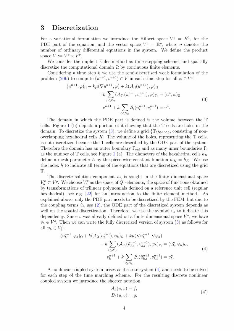
Considering a time step k we use the semi-discretized weak formulation of theproblem (20b) to compute (un+1, vn+1) ∈ V in each time step for all ϕ ∈ V p:

(un+1, ϕ)Ω + kµ(∇un+1, ϕ) + k(AΩ(un+1), ϕ)Ω

+k∑i≤NC

(AΓi(un+1, vn+1

i ), ϕ)Γi= (un, ϕ)Ω,

vn+1 + k∑i≤NC

Bi(un+1i , vn+1

i ) = vn.

(3)

The domain in which the PDE part is defined is the volume between the Tcells. Figure 1 (b) depicts a portion of it showing that the T cells are holes in thedomain. To discretize the system (3), we define a grid Tl0≤l≤L, consisting of non-overlapping hexahedral cells K. The volume of the holes, representing the T cells,is not discretized because the T cells are described by the ODE part of the system.Therefore the domain has an outer boundary Γout and as many inner boundaries Γias the number of T cells, see Figure 1 (a). The diameters of the hexahedral cells hKdefine a mesh parameter h by the piece-wise constant function h|K = hK . We usethe index h to indicate all terms of the equations that are discretized using the gridT.

The discrete solution component uh is sought in the finite dimensional spaceV ph ⊂ V p. We choose V p

h as the space of Q1-elements, the space of functions obtainedby transformations of trilinear polynomials defined on a reference unit cell (regularhexahedral), see e.g. [22] for an introduction to the finite element method. Asexplained above, only the PDE part needs to be discretized by the FEM, but due tothe coupling terms ui, see (2), the ODE part of the discretized system depends aswell on the spatial discretization. Therefore, we use the symbol vh to indicate thisdependency. Since v was already defined on a finite dimensional space V o, we havevh ∈ V o. Then we can write the fully discretized version of system (3) as follows forall ϕh ∈ V p

h :

(un+1h , ϕh)Ω + k(AΩ(un+1

h ), ϕh)Ω + kµ(∇un+1h ,∇ϕh)

+k∑i≤NC

(AΓi(un+1

h,i , vn+1h,i ), ϕh)Γi

= (unh, ϕh)Ω,

vn+1h + k

∑i≤NC

Bi(un+1h,i , v

n+1h,i ) = vnh .

(4)

A nonlinear coupled system arises as discrete system (4) and needs to be solvedfor each step of the time marching scheme. For the resulting discrete nonlinearcoupled system we introduce the shorter notation

Ah(u, v) = f,

Bh(u, v) = g.(4′)

4

We use the subscript h to indicate the dependence of the operator Bh on the meshdiscretization through the coupling with the PDE part. We omit the subscript h forthe solution components u and v to simplify the notation in the next sections.

4 Sensitivity Analysis of the Coupled System

In this section we study the strength of the coupling between the PDE and the ODEpart of the system. This is done to motivate the choice of the solution process thatwe present in the following part of the work. In this work we refer to strong orweak coupling meaning the strength of the coupling independently of the approachused to solve the coupled problem. We first define in the next subsection the useddefinition of strong and weak coupling, then we apply this definition to our systemof equations.

4.1 A criterion to measure the coupling strength

Let Sh : v 7→ u and Th : u 7→ v denote the solution operator for the PDE partand respectively for the ODE part of the discretized system of equations (4′). Thefirst equation, u = Sh(v), is solved for a given value of v, then the second equation,v = Th(u), is solved with the resulting value of u and the cycle is iterated until agiven tolerance is reached. This process can also be written as a composition of thetwo operators:

un+1 = Sh(Th(u

n)). (5)

A fixed-point iteration to solve a coupled system of equations has a slow conver-gence rate (typically only linear) and the number of fixed-point iterations depends onthe nature of the coupling and the model parameters. Considering the formulation(5) to solve our coupled system we write the Jacobian of the fixed-point operator as

J =∂Sh∂v

∂Th∂u

. (6)

For convergence the fixed-point iteration (5) has to fulfill the following criterionaccording to the Banach fixed-point theorem

‖J‖ < 1, (7)

in some norm ‖ · ‖. A more convenient criterion is the substitution of the norm withthe spectral radius of the matrix J

|λmax(J)| < 1. (8)

Based on this statement Haftka and coworkers have defined in [23] a quantitativemeasure for the strength of the coupling between the two parts of the problem. Infact, according to their definition a system is weakly coupled if

|λmax(J)| 1, (9)

5

respectively is strongly coupled if

|λmax(J)| 1. (10)

In [23] there is no precise separation of the two ranges of weak and strong coupling.We also do not give a quantitative definition of the ranges, because a more generaldefinition should consider many models. The criterion (9), respectively (10), hasbeen used here with the maximal eigenvalue of (6) to define whether the couplingof our system is weak, respectively strong, considering that in one case the maximaleigenvalue is two orders of magnitude smaller than 1 and in the other case almostone order of magnitude larger than 1, see results in Section 6.

We remark that in case of nonlinear problems the strength of the coupling couldbe time dependent. In particular, this is the case if the coefficients of the operatorare time dependent. In our case, the coefficients are constant.

4.2 Application to the PDE/ODE coupled system of equa-tions

In the rest of this section we present the sensitivity approach needed to calculate thelargest eigenvalue of the Jacobian J of the fixed-point problem, see (6). Therefore, wedifferentiate the discretized operators Ah and Bh and obtain the sensitivity equations

A′h,u(u, v)uδv + A′h,v(u, v)δv = 0, ∀δv ∈ V o, (11)

and

B′h,v(u, v)vδu +B′h,u(u, v)δu = 0, ∀δu ∈ V ph . (12)

where we have used the notation

uδv :=∂u

∂v(δv), vδu =

∂v

∂u(δu)

for the sensitivities. In the decoupled system, uδv indicates the variation of thePDE solution perturbing the solution of the ODE system and equivalently vδu is thevariation of the ODE system for a perturbation of the PDE system. For nonlinearsystems of equations the sensitivity analysis depends on a given point of lineariza-tion (u, v). We compute an approximate numerical solution of the system (4′) forcharacteristic values of the parameters and choose the computed solution as pointof linearization.

Since the sensitivities in the linear solver strongly depend on the used timestepping scheme, we consider only the sensitivities for a computation of the steadystate. Then, the equations (11) are stationary PDEs to be solved for each componentof δv, while the ODE part (12) consists of algebraic equations solved for each δu.Therefore, we compute the sensitivity matrices ∂Sh/∂v as a N o × Np matrix and∂Th/∂u as a Np×N o matrix, where N o denotes the number of ODE equations andNp the dimension of the PDE discretization.

The sensitivity matrices are

∂Sh∂v

=

(∂u

∂v1

. . .∂u

∂vi. . .

∂u

∂vNo

)T, (13)

6

where each row

(∂u

∂vi

)Tis of the dimension of the PDE discretization and

∂Th∂u

=

∂v1

∂u1

. . .∂vi∂u1

. . .∂vNo

∂u1

. . . . . . . . . . . . . . .

∂v1

∂ui. . .

∂vi∂ui

. . .∂vNo

∂ui. . . . . . . . . . . . . . .

∂v1

∂uNp

. . .∂vi∂uNp

. . .∂vNo

∂uNp

, (14)

where∂vi∂uj

denotes the derivatives of the ith component of v with respect to the jth

degree of freedom of u.

Practical realization In the PDE/ODE system presented in Section 6 the cou-pling between the two parts appears only at the boundaries Γi and only with thefirst two components of v. Thus the product ∂Sh/∂v ∂Th/∂u decouples into a blockdiagonal matrix consisting of 2× 2 matrices for each biological cell. In addition, weneed to calculate the sensitivities (12) only for the restriction of δu on the boundariesΓi, which are nonetheless algebraic equations, so that the major costs to calculatethe sensitivities are given by the PDE part (11).

5 Numerical Schemes

In this section we present two different approaches to solve the class of coupledPDE/ODE systems presented in this work that are depicted in Figure 2. In bothschemes we consider a Newton-type solver for the nonlinearities. In the couplingscheme (a) the linear system is solved by a Krylov-solver that is preconditioned by amultigrid scheme. In the decoupling scheme (b) the Newton update is approximatedby a fixed-point iteration and a multigrid method is applied only to the PDE part.Therefore, the decoupling approach is applied not to the original system but to itslinearization within a Newton step.

This section is organized as follows: we first introduce the nonlinear solver basedon a (Quasi-)Newton method in Subsection 5.1 and then we present the variants ofmultigrid preconditioner in Subsections 5.2 and 5.3.

7

Figure 2: Schematic representation of the considered coupling and decouplingschemes

(a) Coupling scheme

Newton method

↓Krylov-solver for system (15)

↓Multigrid-preconditioner

↓Smoother S1 or S2

(b) Decoupling scheme

Quasi-Newton method

↓Fixed-point iteration for system (16)

Direct solver Krylov-solver

↓Multigrid-preconditioner

↓PDE Smoother

5.1 Nonlinear solver

Newton-type methods provide a flexible and reliable framework for nonlinear prob-lems by solving a series of linear equations. As explained above, we present a fullycoupling and a decoupling approach to solve the linearized subproblems.

5.1.1 Fully coupling Newton’s method

To apply Newton’s method we linearize the system and solve in each Newton stepthe system:(

A′h,u(un, vn) A′h,v(u

n, vn)B′h,u(u

n, vn) B′h,v(un, vn)

)(δun+1

δvn+1

)=

(f − Ah(un, vn)g −Bh(u

n, vn)

), (15)

to obtain the Newton updates δun+1 and δvn+1, with which we calculate the nextiterates un+1 = un + δvn and vn+1 = vn + δvn+1. We write A′h,u and A′h,v for thederivatives of Ah with respect to u and v and analogously B′h,u and B′h,v for thederivatives of Bh.

5.1.2 Decoupling inexact Newton’s method

Secondly we consider a decoupling solving scheme for the linear systems defined ineach Newton-step. For each Newton step n the decoupled system is solved by thefollowing fixed-point iteration(

A′h,u(un, vn) A′h,v(u

n, vn)0 B′h,v(u

n, vn)

)(δui+1

δvi+1

)=

(f − Ah(un, vn)

g −Bh(un, vn)−B′h,v(un, vn)δui

)(16)

until the Newton updates (δui+1, δvi+1) fulfill the linear residual of the system (15)to an accuracy (TOLiter).

If the linear system is solved until the full accuracy is reached then the updateformula (16) defines a full Newton-step, which is equivalent to the exact solution

8

of (15). A common approach to accelerate the computation of the Newton-updatesis a Quasi-Newton iteration in which the Jacobian matrix is approximated only upto a certain accuracy. This corresponds not to solving the system (16) to the fullaccuracy. In this way the costs per Newton iteration are reduced, while the numberof Newton iterations increases. A trade-off between accuracy and total costs canenable a reduction of computing time with respect to a full Newton method. Such aQuasi-Newton scheme is obtained if a low accuracy (TOLiter) or a small maximumnumber of fixed-point iterations (MAX iter) is chosen in the Algorithm 1.

Algorithm 1: Decoupling algorithm: Inexact Newton scheme

n = 0repeat

i = 0repeat

compute Newton updates (δui+1, δvi+1) by solving (16)evaluate the residual resiter of the linear system (15)i = i+ 1

until resiter < TOLiter or i = MAX iter

update the iterate un and vn by δun+1 and δvn+1

evaluate the residual resnewton of the nonlinear system (4′)n = n+ 1

until resnewton < TOLnewton

This decoupling method is compared for different parameters in numerical testsof Section 6.2 to the fully coupling Newton method.

5.2 Multigrid scheme for the coupling approach

In this section we introduce a multilevel preconditioner which can cope with thestrong coupling between PDE and ODEs. Such a coupling arises in the solver of thelinear subsystems if the fully coupling Newton method is used instead of a decouplingscheme. Coupled problems are commonly preconditioned by block preconditioningapproaches, e.g. by simple block diagonal methods or a preconditioning of the Schurcomplement [24]. We will not use a block preconditioning approach because of thesmall dimension of the ODE part but instead we set up a coupling preconditionerbased on the linear multigrid method.

In fact, it is well known that the most efficient preconditioner for the PDEblock is a multilevel preconditioner, because the number of linear iterations becomesindependent of the mesh refinement [25, 7]. We consider a hierarchy of meshesTl0≤l≤L, where the index 0 denotes the root mesh, i.e. the coarsest mesh fromwhich all other meshes are derived by refinement. In this section we use the followingnotation for the system matrix of (15):

Kl :=

(A′,lh,u A′,lh,vB′h,u B′h,v

), (17)

where the index l indicates the grid refinement level. The diagonal block B′h,v doesnot depend on the mesh level, whereas the block B′h,u does depend on the mesh

9

level through the coupling term uh on the cell boundary. Nevertheless, we do notuse the notation with superscript l in the blocks of the ODE part. In fact, we usean approximation in the coupling. To reduce the computational costs and simplifythe implementation, the coupling ODE/PDE block is calculated at each level withthe term uh computed at the finest level. In this way the whole ODE part does notdepend on the refinement level l. Our numerical results have indicated that thismodification does not influence the performance of the multilevel algorithm.

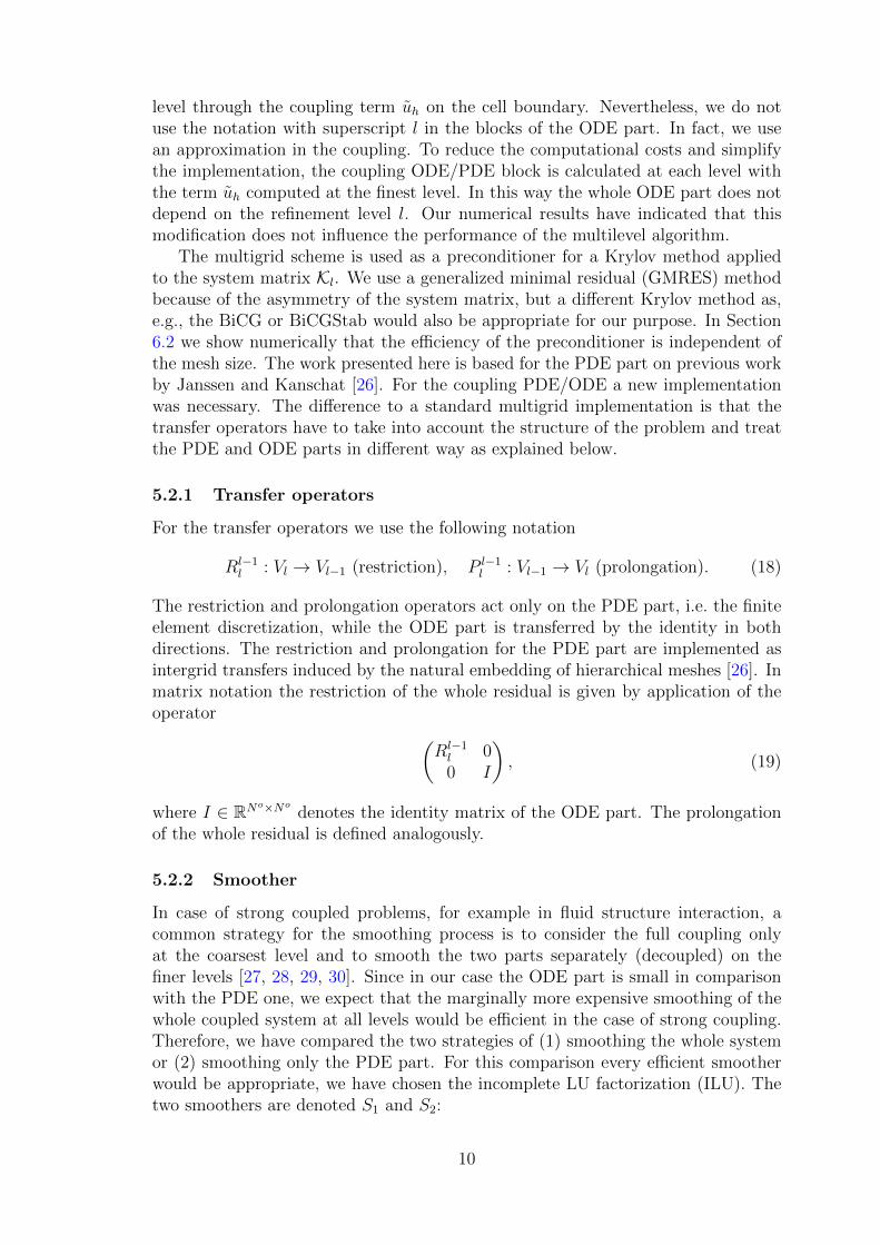
The multigrid scheme is used as a preconditioner for a Krylov method appliedto the system matrix Kl. We use a generalized minimal residual (GMRES) methodbecause of the asymmetry of the system matrix, but a different Krylov method as,e.g., the BiCG or BiCGStab would also be appropriate for our purpose. In Section6.2 we show numerically that the efficiency of the preconditioner is independent ofthe mesh size. The work presented here is based for the PDE part on previous workby Janssen and Kanschat [26]. For the coupling PDE/ODE a new implementationwas necessary. The difference to a standard multigrid implementation is that thetransfer operators have to take into account the structure of the problem and treatthe PDE and ODE parts in different way as explained below.

5.2.1 Transfer operators

For the transfer operators we use the following notation

Rl−1l : Vl → Vl−1 (restriction), P l−1

l : Vl−1 → Vl (prolongation). (18)

The restriction and prolongation operators act only on the PDE part, i.e. the finiteelement discretization, while the ODE part is transferred by the identity in bothdirections. The restriction and prolongation for the PDE part are implemented asintergrid transfers induced by the natural embedding of hierarchical meshes [26]. Inmatrix notation the restriction of the whole residual is given by application of theoperator (

Rl−1l 00 I

), (19)

where I ∈ RNo×Nodenotes the identity matrix of the ODE part. The prolongation

of the whole residual is defined analogously.

5.2.2 Smoother

In case of strong coupled problems, for example in fluid structure interaction, acommon strategy for the smoothing process is to consider the full coupling onlyat the coarsest level and to smooth the two parts separately (decoupled) on thefiner levels [27, 28, 29, 30]. Since in our case the ODE part is small in comparisonwith the PDE one, we expect that the marginally more expensive smoothing of thewhole coupled system at all levels would be efficient in the case of strong coupling.Therefore, we have compared the two strategies of (1) smoothing the whole systemor (2) smoothing only the PDE part. For this comparison every efficient smootherwould be appropriate, we have chosen the incomplete LU factorization (ILU). Thetwo smoothers are denoted S1 and S2:

10

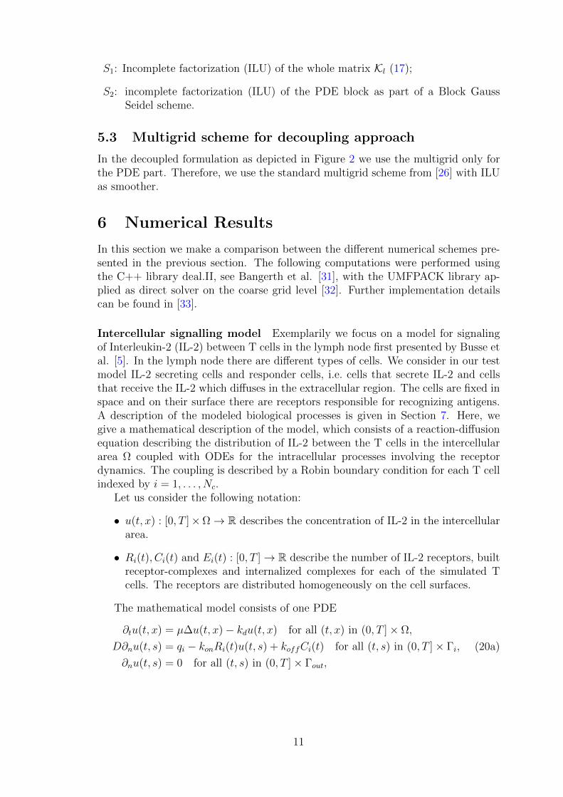
S1: Incomplete factorization (ILU) of the whole matrix Kl (17);

S2: incomplete factorization (ILU) of the PDE block as part of a Block GaussSeidel scheme.

5.3 Multigrid scheme for decoupling approach

In the decoupled formulation as depicted in Figure 2 we use the multigrid only forthe PDE part. Therefore, we use the standard multigrid scheme from [26] with ILUas smoother.

6 Numerical Results

In this section we make a comparison between the different numerical schemes pre-sented in the previous section. The following computations were performed usingthe C++ library deal.II, see Bangerth et al. [31], with the UMFPACK library ap-plied as direct solver on the coarse grid level [32]. Further implementation detailscan be found in [33].

Intercellular signalling model Exemplarily we focus on a model for signalingof Interleukin-2 (IL-2) between T cells in the lymph node first presented by Busse etal. [5]. In the lymph node there are different types of cells. We consider in our testmodel IL-2 secreting cells and responder cells, i.e. cells that secrete IL-2 and cellsthat receive the IL-2 which diffuses in the extracellular region. The cells are fixed inspace and on their surface there are receptors responsible for recognizing antigens.A description of the modeled biological processes is given in Section 7. Here, wegive a mathematical description of the model, which consists of a reaction-diffusionequation describing the distribution of IL-2 between the T cells in the intercellulararea Ω coupled with ODEs for the intracellular processes involving the receptordynamics. The coupling is described by a Robin boundary condition for each T cellindexed by i = 1, . . . , Nc.

Let us consider the following notation:

• u(t, x) : [0, T ]×Ω→ R describes the concentration of IL-2 in the intercellulararea.

• Ri(t), Ci(t) and Ei(t) : [0, T ]→ R describe the number of IL-2 receptors, builtreceptor-complexes and internalized complexes for each of the simulated Tcells. The receptors are distributed homogeneously on the cell surfaces.

The mathematical model consists of one PDE

∂tu(t, x) = µ∆u(t, x)− kdu(t, x) for all (t, x) in (0, T ]× Ω,

D∂nu(t, s) = qi − konRi(t)u(t, s) + koffCi(t) for all (t, s) in (0, T ]× Γi,

∂nu(t, s) = 0 for all (t, s) in (0, T ]× Γout,

(20a)

11

coupled with three ODEs for each T cell

∂tRi(t) = w0i + w1

i

Ci(t)3

K3 + Ci(t)3− konRi(t)ui(t)

− kiRRi(t) + koffCi(t) + krecEi(t) for all cells i = 1, . . . , Nc,

∂tCi(t) = konRi(t)ui(t)− (koff + kiB)Ci(t),

∂tEi(t) = kiBCi(t)− (krec + kdeg)Ei(t),

ui(t) =

∫Γiu(t, s) ds

|Γi|,

(20b)

with given initial conditions for u(0), Ri(0), Ci(0) and Ei(0) for all cells i = 1, . . . , Nc.The used parameters and their values are described in Table 1. The parameters andthe chosen initial values have been taken from [5]. The two types of cell that we

Table 1: Model parameters

Symbol Value Parameter

qi 0− 22000 mol./cell/h IL-2 secretion rateµ 36000 µm2/h Diffusion coefficient of IL-2kd 0,1/h Extracellular IL-2 degradationw0i 150 mol./cell/h Antigen stimulated IL-2 receptor expression rate

w1i 3000 mol./cell/h Feedback induced IL-2 receptor expression rate

K 1000 mol./cell Half-saturation constant of feedback expressionkon 111,6 /nM/h IL-2 association rate constant to IL-2 receptorskoff 0,83/h IL-2 dissociation rate constant from IL-2 receptorskiR 0,64/h Internalization rate constant of IL-2 receptorskiC 1,7/h Internalization rate constant of receptor complexeskrec 9/h Recycling rate constant of IL-2 receptorskdeg 5/h Endosomal degradation constant IL-2 receptorsr 5µm Cell radiusd 5µm Cell to cell distance

consider share the same receptor dynamics but differ in the IL-2 secretion rate:

• Secreting T cells, which secrete IL-2 with the secretion rate qi = 2500 mol/h,

• Responding T cells with qi = 0.

Table 2: Value of the IL-2 degradation parameter and corresponding maximumeigenvalue of J , see (6)

kd λmaxBiologically relevant test model 0.1 8.8

Artificial test model 1000 0.01

In Section 7 we show a simulation for a microenvironment configuration with 216T cells, among them 54 randomly chosen secreting T cells. That simulation is used

12

to give a biological interpretation to the results obtained with the presented model.The numerical tests shown here are performed using a subproblem. We consideronly eight cells among them only one is secreting IL-2. The reduction in size allowsfor fast tests and does not affect the study of the strength of the coupling. In fact, wehave observed by calculations using many different configurations that the strengthof the coupling depends on the model parameters and not on the number of cells.The configuration is displayed in Figure 1 where the responding T cells are in greyand the secreting T cell is highlighted. For this test problem we found a stationarystate numerically.

The goal of the next subsections is to show the numerical comparison between thetwo schemes depicted in Figure 2. We have divided the results in three subsections:

• Subsection 6.1: at first we compare the two smoothers S1 and S2 that we havechosen for the coupling solver, see again Figure 2.

Once we have decided which is the best smoother for the coupling solver, we comparethis solver with the decoupling solver in two cases:

• Subsection 6.2: the stationary case;

• Subsection 6.3: the non-stationary case.

Since the results depend on the strength of the coupling, we want to test oursolvers for strong and weak coupling conditions for both the stationary and thenon-stationary cases. In the stationary case, we consider two configurations chang-ing the parameter kd. The two values of kd and the respective maximal eigenvaluesof the Jacobian are shown in Table 2. We denote the case with low value of kdas biologically relevant since it is in the range of reference values given in Table 1.According to the criterion (10) it is a strongly coupled system.

We refer to the case with a high value of kd as an artificial setting since thisvalue is far larger than the biological assumptions taken in other publications withthis model [5, 34]. According to the criterion (9) it is a weakly coupled system. Highvalues of kd correspond to large degradation of u. In this way the influence of v onu is diminished. Thus the PDE part is artificially decoupled from the ODE part.We use the two proposed settings to compare the solvers. In the next paragraphswe give a biological interpretation of the two settings.

Biological scenario for the strongly coupled (biological relevant) testmodel This model consists of 8 T cells among which one is a secreting cell. Allparameters are like in the real application, in the lymph node (Table 1). After thedefinition in (10) we have a strongly coupling between the equations. In Figure 3(a) we see the time course of the IL-2R receptors (the sum of R and C receptors) onthe surface of each cell. The receptors need some minutes to get the IL-2 for a slightincrease and reach their steady state quite early after 9 hours. In this configurationone secreting cell is not enough to activate the others. In Figure 3 (b) we see thetime course of the averaged IL-2. Again we have a slight increase in the first 3 hoursand the steady state regulates quite early after 9 hours. The IL-2 concentration islow, around 0.045 pM.

13

Figure 3: Dynamic behavior for the biological relevant test model which is stronglycoupled (8 T cells among them one secreting)

0 5 10 15 20230

240

250

260

270

280

time (h)

IL−

2R (

mol

ecul

es/c

ell)

(a) Time course of the amount of IL-2R receptors (R+C) on thesurface of each cell. No cell is activated in this configuration

0 5 10 15 200

0.01

0.02

0.03

0.04

0.05

0.06

time (h)

IL−

2 (p

M)

(b) Time course of the averaged IL-2 concentration on the surface ofall cells

Biological scenario for the weakly coupled (artificial) test model Thismodel differs from the biological relevant test model only in one parameter, kd , thedegradation rate. The parameter is chosen artificially to create a weekly couplingbetween the equations. It is chosen to be greater by four orders of magnitude withrespect to the biologically relevant value (Table 2). Therefore, IL-2 degrades 104

faster than in the strongly coupled scenario. It follows that there is much less IL-2available for the responder cells than in the strongly coupled model. Numericalsimulations (Figure 4) show that the amount of IL-2 is reduced by three orders ofmagnitude. Thus, there will be less IL-2 for the responder cells and also no chancefor activation. In the steady state which occurs immediately, whereas in the strongly

14

coupled model it occurs after 9 hours, there is only 2.2 ·10−4 pM IL-2 which is threeorders of magnitude less than in the biological relevant scenario. The total amountof IL-2R receptors stays almost constant for all times. With this concentrationchanges in the ODEs the secreting cell also produces less IL-2.

In the non-stationary case, we do not have to change kd to compare two config-urations. Instead we use two different time discretizations with steps ∆t = 0.01hand ∆t = 0.1h. By reducing the time step in this way we also reduce the strengthof the coupling as shown in the results.

Figure 4: Dynamic behavior for the artificial test model which is weekly coupled (8T cells among them one secreting)

0 5 10 15 20

234

234.2

234.4

234.6

234.8

235

time (h)

IL−

2R (

mol

ecul

es/c

ell)

(a) Time course of the amount of IL-2R receptors (R+C) on thesurface of each cell. No cell is activated in this configuration

0 5 10 15 200

1

2

3

4x 10

−4

time (h)

IL−

2 (p

M)

(b) Time course of the averaged IL-2 concentration on the surface ofall cells

15

6.1 Choice of multigrid preconditioner for the coupling solver

The two smoothers have been described in Subsection 5.2.2. We compare them usingthe configuration with a strong coupling strength, i.e. the biologically relevant case.Recall that S1 uses a factorization of the whole matrix, while S2 uses a factorizationof only the PDE part.

We compute the number of GMRES steps over all Newton steps (Σn) and theaverage reduction rate (r) of the residual in each GMRES step. We have set theNewton accuracy to 10−6. The accuracy of the linear solver per Newton step isset to 10−11. We have observed that the number of Newton steps only depends onthe coupling, the nonlinearity of the equation and the accuracy of the solver. Inparticular it is not dependent on the grid refinement. The latter effect is knownas “asymptotic mesh independence” and a proof of it can be found in [35, 36] forNewton-type methods applied to nonlinear operator equations and, e.g., in [37] fora Gauss-Newton method for nonlinear Least Squares problems. The number ofsmoothing cycles are set in both smoothers to three. We have observed that a largernumber of smoothing steps is unnecessary to improve the smoother performance.To test the mesh independence of the multigrid preconditioner we compute severalrefinement levels up to five refinements as indicated in the first column of Table3. We use a global refinement of the grid. The finest grid has 885673 degrees offreedom, the coarsest 367 degrees of freedom for the PDE part. Additionally 24degrees of freedom for the ODE part are coupled to the PDE part. Table 3 showsthat the number of GMRES steps preconditioned by the two smoothers is almostconstant for S1 (from 46 at L = 2 to 54 at L = 5) and increases moderately for S2

(from 69 at L = 2 to 84 at L = 5). Therefore we have chosen S1 because it is meshindependent and more effective. In fact, the computational costs per smoothingiteration are almost the same for the two smoothers because the ODE block is notlarge. Since the costs are comparable, we see that the smoother S1 costs from 33%(at L = 2) to 35% (at L = 5) less than the smoother S2.

Table 3: Reduction rates of different preconditioners

MG-S1 (ILU) MG-S2 (Bl.-ILU)

L log10 r Σs log10r Σs2 2.00 46 1.41 693 1.92 51 1.27 774 1.85 54 1.21 815 1.81 54 1.15 84

Notation: Σs GMRES iterationsin all Newton steps

r average reduction rateL refinement level

6.2 Stationary case

In this section we compare the two approaches depicted in Figure 2 where for thecoupling method (a) we use the smoother S1 as explained above. For the coupling

16

approach we use an iterative method preconditioned by the multigrid method de-scribed in 5.2, while for the decoupling approach we use the method described in5.3. In the coupled case, since the matrix is asymmetric we use a GMRES method.In the decoupling approach the system matrix is symmetric, therefore the solverof choice would be, e.g. the conjugate gradient method (CG). Nevertheless, for adirect comparison we use instead the GMRES method also for this approach. Infact, we have observed that, in combination with the preconditioner, both solvershave similar performance. Furthermore, to make the schemes comparable we usethe same accuracy of the GMRES solver set to TOLiter for both schemes. In thisway the number of Newton steps to solve the nonlinear problem is independent ofthe approach and we can compare the total number of GMRES steps to solve for aNewton accuracy of TOLnewton.

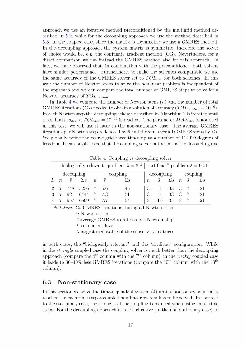
In Table 4 we compare the number of Newton steps (n) and the number of totalGMRES iterations (Σs) needed to obtain a solution of accuracy (TOLnewton = 10−6).In each Newton step the decoupling scheme described in Algorithm 1 is iterated untila residual resiter < TOLiter = 10−11 is reached. The parameter MAX iter is not usedin this test, we will use it later in the non-stationary case. The average GMRESiterations per Newton step is denoted by s and the sum over all GMRES steps by Σs.We globally refine the coarse grid three times up to a number of 114929 degrees offreedom. It can be observed that the coupling solver outperforms the decoupling one

Table 4: Coupling vs decoupling solver

“biologically relevant” problem λ = 8.8 “artificial” problem λ = 0.01

decoupling coupling decoupling couplingL n s Σs n s Σs n s Σs n s Σs

2 7 748 5236 7 6.6 46 3 11 33 3 7 213 7 921 6444 7 7.3 51 3 11 33 3 7 214 7 957 6699 7 7.7 54 3 11.7 35 3 7 21

Notation: Σs GMRES iterations during all Newton stepsn Newton stepss average GMRES iterations per Newton stepL refinement levelλ largest eigenvalue of the sensitivity matrices

in both cases, the “biologically relevant” and the “artificial” configuration. Whilein the strongly coupled case the coupling solver is much better than the decouplingapproach (compare the 4th column with the 7th column), in the weakly coupled caseit leads to 30–40% less GMRES iterations (compare the 10th column with the 13th

column).

6.3 Non-stationary case

In this section we solve the time-dependent system (4) until a stationary solution isreached. In each time step a coupled non-linear system has to be solved. In contrastto the stationary case, the strength of the coupling is reduced when using small timesteps. For the decoupling approach it is less effective (in the non-stationary case) to

17

solve the linear problems up to a very small tolerance (TOLiter) as can be seen fromthe numerical results. For this reason we have introduced the parameter MAX iter

in Algorithm 1, and for comparison purposes we have made numerical tests with thevalues MAX iter = 1, . . . , 4, see first column in Table 5. This table reports as well

Table 5: Decoupling and coupling solving of the non-stationary problem

∆t = 0.1h ∆t = 0.01hMAX iter Σn Σs Σn Σs

decoupling 1 1393 3375 5566 140162 754 3792 3395 152173 547 4363 2880 211534 448 4775 2871 23658

coupling 356 1799 2868 11299

Notation: Σn Newton steps in all time stepsΣs Krylow iterations in all Newton stepsMAX iter maximum of iterations

per Newton step

the sum of computed newton steps (Σn) and the sum of computed GMRES steps(Σs) over all time steps. The results are listed for computations on a spatial gridlevel L = 2 (2189 degrees of freedom) with 200 (∆t = 0.1h) or 2000 (∆t = 0.01h)time steps, with final time 20 hours.

A higher maximal number of fixed-point iterations per Newton step (i.e. a higherMAX iter) increases the accuracy of the linear solver and thus reduces the numberof Newton steps. The decoupling solving scheme with a MAX iter = 4 results ina number of Newton steps not much larger than in coupling solving scheme (448vs 356) but with more than twice the number of computed GMRES steps (4775vs 1799). Furthermore, it can be observed that the number of total GMRES stepsdecreases reducing MAX iter, see the 3rd column. A comparison of the computationaltime should consider also the time per Newton step. In fact, we observe that thecomputing time for solving with the decoupling approach is much larger than thedouble of the time needed by the coupling approach. In fact, associated to eachNewton iteration there are additional computational costs, e.g. building or updatingthe Jacobian and the residual. Since the time per Newton step depends on thespecific implementation (e.g. how often the Jacobian is updated), we restrict thecomparison to the total number of linear solving. For this reason we consider abetter choice the value of MAX iter = 1.

As already remarked, the effectiveness of the decoupling solver depends on thestrength of the coupling and thus on the size of the time step. In fact the couplingsolver needs for time steps ∆t = 0.1h around half of the iterations of the decouplingsolver, while for smaller time steps (∆t = 0.01h) the iterations of the coupling solverare reduced by 20% compared to the decoupling solver with MAX iter = 1.

Remark 6.1. By using the implicit Euler scheme we have shown that the couplingsolver is more effective. The use of a higher order time scheme, e.g. the Crank-Nicolson scheme, allows for larger time steps to produce the same accuracy. Asshown above, larger time steps lead to a stronger coupling during the time integration.

18

We expect therefore that the coupling solver is even more effective using a higherorder time scheme.

Remark 6.2. For the test that we have done in this work we did not use a global-ization method for the Newton convergence. Our experience is that for the dynamicproblem we do not need globalization, while for the stationary problem some criticalconfigurations could be solved only using pseudo time steps approach to get a goodstart solution for Newton to converge.

Solver performance with increasing number of T cells To test how thesolver scales with the number of T cells, i.e. how the total number of Newton stepsand the total number of GMRES steps increase with the increasing number of thesimulated T cells, we have run simulations with 8, 27 and 64 T cells. The parameterset is the same as that for the previous simulations, in particular we set the final timeto 20 hours and a time step ∆t = 0.1h. To maintain the same ratio between secretingand responding T cells, around 1/8 of the total number of T cells is randomly chosenas secreting, i.e. 1, 3, and 8 for the simulations with 8, 27 and 64 T cells respectively.Since the computing time for the decoupling solver is much larger than that for thecoupling solver, we have run the simulations at refinement level L = 1.

In Table 6 we report the total number of Newton steps and the total number ofGMRES steps for all time steps. For the coupled problem we use the notation ΣnCand ΣsC and for the decoupling solver the notation ΣnD and ΣsD. The last columnshows the reduction of total GMRES steps by using the coupling solver with respectto the decoupling one. It can be observed that the gain of the coupling solver scalesperfectly with the number of T cells, i.e. the reduction of total number of GMRESsteps by using the coupling solver is around 50% independently of the number of Tcells.

Table 6: Scaling with the number of T cells

Coupling Decoupling Reduction of ΣsNum. T cells ΣnC ΣsC ΣnD ΣsD ΣsC/ΣsD

8 337 1601 1250 2997 53%27 334 2007 1214 3389 59%64 344 2316 1343 4386 52%125 345 2672 1325 4813 55%

Notation: Σn Newton steps in all time stepsΣs Krylow iterations in all Newton steps

7 Application to a cellular microenviroenment

We present a numerical result applied to a cellular microenvironment consisting of216 T cells. This in silico experiment can be considered as representative to observethe cell-to-cell interactions in the lymph node. In our configuration 54 T cells arerandomly chosen as T helper cells and release IL-2 locally into the immunologicalsynapse with a rate of qi = 3500 mol/h. The remaining cells are responding T cells

19

with qi = 0 which absorb the IL-2 from the environment. The amount of IL-2 whichis absorbed by each cell is proportional to the number of the expressed receptorson their surface and this number depends again on the amount of absorbed IL-2.This means, the more IL-2 a cell can absorb the more receptors are expressed onits surface. If a certain amount of receptors are expressed, the T cell is activatedand ready for proliferation and differentiation determining the type of the immuneresponse. The more IL-2 a cell absorbs the better is the chance for it to get activated.Thus, the result is a competitive behavior between the cells for IL-2.

For this application we have used a final time of 30 hours, a time step ∆t = 0.1hand a refinement level L = 2. Due to the value of kd = 0.1/h the equations arestrongly coupled. In Figure 5 (a) we see the time development of the amount ofreceptors for each T cell. At the beginning the amount of receptors grows stronglyin all cells with the same speed. After 9 hours they have five times more receptorsthan in the biological relevant test model. Thereafter they split into two groups,the activated (yellow curves) and non-activated (grey curves) cells. A cell is calledactivated when it has more than 4000 IL-2R molecules. After 30 hours the T cellshave either become activated by building new receptors or their number of receptorshas decreased to the starting level. These biological processes take some time suchthat the steady state will be reached later after 30 hours. The Figure 5 (b) showsthe averaged IL-2 concentration at the cell surface. Here, the same colors are used,yellow (see electronic version of the paper for the colors) for the activated and grayfor the non-activated cells. Interestingly, there is almost no difference in the averagedamount of IL-2 between activated and non-activated cells except at the time point ofdecision, i.e. after 9 hours of activation. The cells which get slightly more IL-2 at thistime will be activated. All others will down-regulate their receptors. In the steadystate there is over 100 times more IL-2 than in the corresponding test model withone secreting cell and in the initial phase 104 times more. One of the most importantbiological findings from these simulations was the heterogeneity of the IL-2 amountin time and space. Despite the rapid diffusion of IL-2, spatial inhomogeneities occurin the concentration distribution (Figure 6) and large gradients develop over severalorders of magnitude (Figure 5 (b)). In Figure 6 we present a volume visualization ofour numerical results for the chosen configuration in the steady state performed withCovise [38]. Transparency of the whole data set is used to make the inner structurevisible and a flexible mapping of the data on colors and opacity to visualize thedifferent T cells for a realistic representation. The (randomly) chosen secreting cellsare marked with magenta (see color version of the paper). By visualizing only apart of the IL-2 range we can see the secretion points on the cell surfaces (small reddomains). There, we find the largest IL-2 concentration. The yellow cells are theactivated cells and the transparent gray ones the responder cells which have down-regulated their receptors. Further visualization and numerical results are presentedin [34].

20

Figure 5: Dynamic behavior of 216 T cells among them 54 secreting T cells

0 5 10 15 20 25 300

1000

2000

3000

4000

5000

time (h)

IL−

2R (

mol

ecul

es/c

ell)

(a) Time course of the amount of IL-2R receptors (R+C) on thesurface of each of the activated (yellow curves) and non-activated

(gray curves) cells

0 5 10 15 20 25 30

10

100

1000

time (h)

IL−

2 (p

M)

(b) Time course of the averaged IL-2 concentration on the surface ofall activated (yellow curve; at t=9h is the curve above) and

non-activated (gray curves) cell surfaces

21

Figure 6: IL-2 concentration distribution in a cell microenvironment consisting of216 T cells. This inhomogeneous IL-2 pattern develops in the steady state after 30hours of activation of the IL-2 signaling pathway

8 Conclusions

In this paper, we considered a coupled nonlinear system consisting of a parabolicpartial differential equation and many ordinary differential equations, which emergese.g. in systems biology by modeling intercellular signaling pathways. We presentednumerical results for an application in immunology: the dynamics of cytokine(Interleukin-2) signaling between different types of T cells. The presented methodscan nevertheless be used for solving other signaling pathways or other applicationsmodeled by systems of coupled PDE/ODE equations.

Previous works dealing with coupled PDE/ODE models have presented mainlydecoupling approaches (especially for biological applications) and have not showna quantitative comparison with coupling approaches (see references in the intro-duction). This paper showed in a systematic way a quantitative comparison be-tween coupling and decoupling approaches for this class of problems. Specifically,we used a sensitivity analysis and its numerical implementation to study the cou-pling/decoupling strategy. This approach, applied to the model for Interleukin-2

22

signaling, indicated that a coupling strategy performs better for our strongly cou-pled model. We implemented a solution method based on a Newton-type solver witha multigrid preconditioner. Depending on the time step length, the total numberof linear solver iterations over all Newton steps can be reduced with this strategyup to 50%. The saving in computational time is typically much more than 50%because also the number of Newton iterations is higher in the decoupling scheme incomparison with the coupling one, and associated to each Newton iteration thereare additional computational costs. Nevertheless, the quantitative estimation of thecomputing time highly depends on how the Newton method is implemented. There-fore, in this work we have restricted the comparison to the total number of linearsolving over all Newton steps.

As future work, we indicate a possible strategy for an additional reduction of thecomputation time by using local mesh refinement both in space and time. In par-ticular, different time grids for the PDE and the ODE part allow, depending on thestrength of the coupling, to decrease the number of time steps for the computation-ally expensive PDE part of the model. The essential question is how to choose thetwo time grids without decreasing the overall convergence rate of the method. An aposteriori error estimator for the errors of the PDE and ODE discretization is neces-sary to reach a wanted accuracy efficiently by iterative adaptive refinement. The useof a refinement strategy based on such an error estimator allows to control the twotime grids separately and obtain an optimal time discretization for both parts of thesystem. The complex realization of such a method is subject of our current research.

AcknowledgementsThe authors thank Prof. Rolf Rannacher for the numerous fruitful discussions on

numerical aspects of this work. Furthermore, the authors acknowledge Prof. ThomasHofer for his support and for provisioning this concrete application in immunology.In addition, the authors gratefully acknowledged the work for the visualization in3D done by Marcus Schaber (Visualization and Numerical Geometry Group at theInterdisciplinary Center of Scientific Computing (IWR), Heidelberg.)T.C. was supported by Deutsche Forschungsgemeinschaft (DFG) through the projectCA 633/2-1.E.F. and D.G. were supported by the Helmholtz Alliance on Systems Biology (SBCancer, Submodule V.7) and D.G. additionally by ViroQuant.

References

[1] H. A. Kestler, C. Wawra, B. Kracher, M. Kuhl, Network modeling of signaltransduction: establishing the global view, Bioessays 30 (11-12) (2008) 1110–1125.

[2] J. Sherratt, P. Maini, W. Jager, W. Muller, A receptor based model for patternformation in hydra, Forma 10 (2) (1995) 77–95.

[3] A. Marciniak-Czochra, Receptor-based models with diffusion-driven instabilityfor pattern formation in hydra, Journal of Biological Systems 11 (03) (2003)293–324.

23

[4] E. Friedmann, A. Pfeifer, R. Neumann, U. Klingmller, R. Rannacher, Inter-action Between Experiment, Modeling and Simulation of Spatial Aspects inthe JAK2/STAT5 Signaling Pathway, in: H. G. Bock, T. Carraro, W. Jager,S. Korkel, R. Rannacher, J. P. Schloder (Eds.), Model Based Parameter Esti-mation, Vol. 4 of Contributions in Mathematical and Computational Sciences,Springer Berlin Heidelberg, 2013, pp. 125–143.

[5] D. Busse, M. de la Rosa, K. Hobiger, K. Thurley, M. Flossdorf, A. Schef-fold, T. Hofer, Competing feedback loops shape IL-2 signaling between helperand regulatory T-lymphocytes in cellular microenvironments, PNAS 107 (2010)3058–3063.

[6] A. Brandt, Multi-level adaptive solutions to boundary-value problems, Mathe-matics of Computation 31 (138) (1977) 333–390.

[7] W. Hackbusch, Multi-grid methods and applications., Springer Series in Com-putational Mathematics, 4. Berlin etc.: Springer- Verlag. XIV, 377, 1985.

[8] D. J. Mavriplis, An assessment of linear versus nonlinear multigrid methods forunstructured mesh solvers, Journal of Computational Physics 175 (1) (2002)302–325.

[9] M. E. Moghadam, I. E. Vignon-Clementel, R. Figliola, A. L. Marsden, A mod-ular numerical method for implicit 0D/3D coupling in cardiovascular finite el-ement simulations, Journal of Computational Physics 244 (0) (2013) 63 – 79.

[10] C. Farhat, M. Lesoinne, Fast staggered algorithms for the solution of three-dimensional nonlinear aeroelastic problems, Numerical Unsteady Aerodynamicsand Aeroelastic Simulation (1998) 7–1.

[11] C. A. Felippa, K. Park, C. Farhat, Partitioned analysis of coupled mechanicalsystems, Computer methods in applied mechanics and engineering 190 (24)(2001) 3247–3270.

[12] D. Mok, W. Wall, Partitioned analysis schemes for the transient interaction ofincompressible flows and nonlinear flexible structures, Trends in computationalstructural mechanics (2001) 689–698.

[13] M. Heil, Stokes flow in an elastic tubea large-displacement fluid-structure in-teraction problem, International journal for numerical methods in fluids 28 (2)(1998) 243–265.

[14] G. Seemann, F. Sachse, M. Karl, D. Weiss, V. Heuveline, O. Dossel, Frameworkfor Modular, Flexible and Efficient Solving the Cardiac Bidomain EquationsUsing PETSc, in: A. D. Fitt, et al. (Eds.), Progress in Industrial Mathematicsat ECMI 2008, Mathematics in Industry, Springer Berlin Heidelberg, 2010, pp.363–369.

[15] M. Cervera, R. Codina, M. Galindo, On the computational efficiency and im-plementation of block-iterative algorithms for nonlinear coupled problems, En-gineering Computations: Int J for Computer-Aided Engineering 13 (6) (1996)4–30.

24

[16] T. Ricken, D. Werner, H. Holzhtter, M. Knig, U. Dahmen, O. Dirsch, Model-ing functionperfusion behavior in liver lobules including tissue, blood, glucose,lactate and glycogen by use of a coupled two-scale PDE-ODE approach, Biome-chanics and Modeling in Mechanobiology 14 (3) (2015) 515–536.

[17] A. Quarteroni, A. Veneziani, Analysis of a Geometrical Multiscale Model Basedon the Coupling of ODE and PDE for Blood Flow Simulations, MultiscaleModeling & Simulation 1 (2) (2003) 173–195.

[18] C. Stinner, C. Surulescu, M. Winkler, Global weak solutions in a pde-ode sys-tem modeling multiscale cancer cell invasion, SIAM Journal on MathematicalAnalysis 46 (3) (2014) 1969–2007.

[19] J. S. Leiva, P. J. Blanco, G. C. Buscaglia, Iterative strong coupling of dimen-sionally heterogeneous models, International Journal for Numerical Methods inEngineering 81 (12) (2010) 1558–1580.

[20] X.-C. Cai, D. E. Keyes, L. Marcinkowski, Nonlinear additive Schwarz precondi-tioners and application in computational fluid dynamics., Int. J. Numer. Meth-ods Fluids 40 (12) (2002) 1463–1470.

[21] A. Quarteroni, A. Valli, Domain decomposition methods for partial differentialequations, Tech. rep., Oxford University Press (1999).

[22] P. G. Ciarlet, The finite element method for elliptic problems., Studies in Math-ematics and its Applications. Vol. 4. Amsterdam - New York - Oxford: North-Holland Publishing Company. (1978).

[23] R. Haftka, J. Sobieszczanski-Sobieski, S. Padula, On options for interdisci-plinary analysis and design optimization, Structural optimization 4 (1992) 65–74.

[24] J. Mandel, On block diagonal and schur complement preconditioning, Nu-merische Mathematik 58 (1) (1990) 79–93.

[25] J. H. Bramble, Multigrid Methods, Longman Scientific and Technical, London,1993.

[26] B. Janssen, G. Kanschat, Adaptive multilevel methods with local smoothingfor h1- and hcurl-conforming high order finite element methods, SIAM J. Sci.Comput. 33 (2011) 2095–2114.

[27] E. van Brummelen, K. van der Zee, R. de Borst, Space/time multigrid for afluid-structure-interaction problem, Applied Numerical Mathematics 58 (12)(2008) 1951 – 1971, special Issue in Honor of Piet Hemker.

[28] M. W. Gee, U. Kttler, W. A. Wall, Truly monolithic algebraic multigrid forfluidstructure interaction, International Journal for Numerical Methods in En-gineering 85 (8) (2011) 987–1016.

[29] Y. Langer, A note on robust preconditioners for monolithic fluid-structure in-teraction systems of finite element equations (2014).URL http://arxiv.org/abs/1412.6845

25

[30] T. Richter, A monolithic geometric multigrid solver for fluid-structure inter-actions in ALE formulation, International Journal for Numerical Methods inEngineering 104 (5) (2015) 372–390.

[31] W. Bangerth, T. Heister, L. Heltai, G. Kanschat, M. Kronbichler, M. Maier,B. Turcksin, T. D. Young, The deal.II library, version 8.2, Archive of Numer-ical Software 3.

[32] T. A. Davis, Algorithm 832: Umfpack v4. 3—an unsymmetric-pattern multi-frontal method, ACM Transactions on Mathematical Software (TOMS) 30 (2)(2004) 196–199.

[33] D. Gerecht, Adaptive finite element simulations of coupled PDE/ODE systemsmodeling intercellular signaling, Ph.D. thesis, Heidelberg University (2015).

[34] K. Thurley, S. C. Tovey, G. Moenke, V. L. Prince, A. Meena, A. P. Thomas,A. Skupin, C. W. Taylor, M. Falcke, Reliable Encoding of Stimulus Intensi-ties Within Random Sequences of Intracellular Ca2+ Spikes, Science Signaling7 (331) (2014) ra59.

[35] M. Weiser, A. Schiela, P. Deuflhard, Asymptotic Mesh Independence of New-ton’s Method Revisited, SIAM Journal on Numerical Analysis 42 (5) (2005)1830–1845.

[36] E. L. Allgower, K. Bohmer, Application of the Mesh Independence Principleto Mesh Refinement Strategies, SIAM Journal on Numerical Analysis 24 (6)(1987) 1335–1351.

[37] M. Heinkenschloss, Mesh Independence for Nonlinear Least Squares Problemswith Norm Constraints, SIAM Journal on Optimization 3 (1) (1993) 81–117.

[38] HLRS High Performance Computing Center Stuttgart, COllaborative VIsual-ization and Simulation Environment (COVISE).URL www.hlrs.de/covise

26