coupling of hydrologic effects to borehole strain data · coupling of hydrologic effects to...

Notes on Hydrologic Coupling 3/27/06

1

Coupling of Hydrologic Effects to Borehole Strain Data

Evelyn Roeloffs, USGS

July 2005

1. Introduction

The entire period range over which borehole strainmeters are useful can be

subdivided into several smaller ranges.

High-frequency data (100 or 200 sps) from some dilatometers and from the mini-

PBO Sakata-type 3-component strainmeters has been recorded and appears to be of good

quality. However, few quantitative comparisons have been made between these data and

seismic recordings. Little or no data has been available from the GTSM’s at sampling

intervals shorter than 5 minutes. 20-sps data from new PBO installations will allow the

performance of these instruments to be investigated in the high-frequency range.

The tidal band was discussed above. It is unusual for a borehole strainmeter to

fail to record any tides. For most dilatometers, agreement between observed and

reference areal strain phases is very good. The situation is not quite so simple for GTSM

shear strains.

However, it is for periods longer than about 10 days that the most challenging

questions arise as to the meaningfulness of borehole strainmeter data. At these periods,

other factors can affect the data, many of which are hydrologic.

Topics covered in this section:

1) Response to rainfall and snow loading

2) Basic poroelastic coupling and fluid flow

3) Direct effects of fluid pressure changes on the strainmeter

4) Hydrologic influences on post-earthquake strain changes.

5) Drainage effects

Hydrologic Effects 3/27/06

2

2. Snow and Rainfall Loading

Borehole strainmeters are sensitive enough to detect the weight of rain or snow on

the earth’s surface. Shallow tiltmeter installations and creepmeters are notoriously

affected by rainfall, often exhibiting large excursions that continue after the rainfall has

stopped, and which are attributable to nonlinear behavior of soft, weathered, near-surface

materials. It is important to understand the the responses to rainfall recorded by borehole

strainmeters installed in rock of low porosity, at depths of 100 meters or more, are of an

entirely different origin and reflect the instrument’s very high sensitivity.

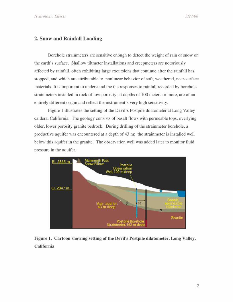
Figure 1 illustrates the setting of the Devil’s Postpile dilatometer at Long Valley

caldera, California. The geology consists of basalt flows with permeable tops, overlying

older, lower porosity granite bedrock. During drilling of the strainmeter borehole, a

productive aquifer was encountered at a depth of 43 m; the strainmeter is installed well

below this aquifer in the granite. The observation well was added later to monitor fluid

pressure in the aquifer.

Figure 1. Cartoon showing setting of the Devil's Postpile dilatometer, Long Valley,

California


3

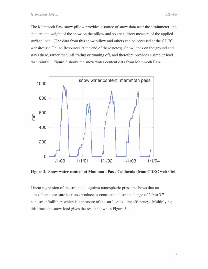
The Mammoth Pass snow pillow provides a source of snow data near the strainmeter; the

data are the weight of the snow on the pillow and so are a direct measure of the applied

surface load. (The data from this snow pillow and others can be accessed at the CDEC

website; see Online Resources at the end of these notes). Snow lands on the ground and

stays there, rather than infiltrating or running off, and therefore provides a simpler load

than rainfall. Figure 2 shows the snow water content data from Mammoth Pass.

0

200

400

600

800

1000

1/1/00 1/1/01 1/1/02 1/1/03 1/1/04

snow water content, mammoth pass

mm

Figure 2. Snow water content at Mammoth Pass, California (from CDEC web site)

Linear regression of the strain data against atmospheric pressure shows that an

atmospheric pressure increase produces a contractional strain change of 2.9 to 3.7

nanostrain/millibar, which is a measure of the surface-loading efficiency. Multiplying

this times the snow load gives the result shown in Figure 3.


4

Figure 3. Snow load component of Postpile strain

At Postpile, the snow load is a small but distinct influence on the strainmeter data.

Because the snow is a static load, it can be corrected for by just removing a scaled

version of the snow water content data. Obviously snow loading is not a large part of the

seasonal cycle at Postpile; we will return to this later.

Like snow, rainfall applies a surface load. However, it does not stay on the

ground above the strainmeter, or accumulate there. So generally rainfall loading steps are

smaller than snow loading steps, and they dissipate over a period of days. If rainfall

loading steps occur, then they usually occur during low values of atmospheric pressure.

Therefore,when determining the strainmeter’s response to atmospheric pressure, it may

be necessary to select a stretch of data without rainfall.

Should rainfall loading show up on GTSM data? Surface loads do produce

horizontal strain, so in principle, rainfall loading can be observed in time series of

individual gauge components, or in areal strain components. Rainfall is not expected to

produce significant shear strain, but should always be evaluated as a possible contributor

to borehole strainmeter signals.

3. Coupling of fluid pressure and strain Subsurface fluid pressure and strain are coupled. The reason is that deforming a

rock changes the volume of pore space. Unless fluid can escape or enter the deformed


5

volume (as it can near the water table), the pore volume change causes the pore fluid

pressure to change. Conversely, fluid-pressure changes in subsurface rocks deform the

rock. Non-uniform fluid pressures generally dissipate with time due to fluid flow, and

therefore the coupled strains are also time-varying.

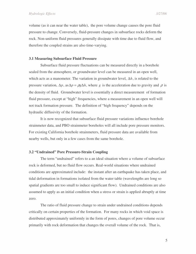
3.1 Measuring Subsurface Fluid Pressure

Subsurface fluid pressure fluctuations can be measured directly in a borehole

sealed from the atmosphere, or groundwater level can be measured in an open well,

which acts as a manometer. The variation in groundwater level, ∆h , is related to the

pressure variation, ∆p , as∆p = ρg∆h , where g is the acceleration due to gravity and ρ is

the density of fluid. Groundwater level is essentially a direct measurement of formation

fluid pressure, except at “high” frequencies, where a measurement in an open well will

not track formation pressure. The definition of “high frequency” depends on the

hydraulic diffusivity of the formation.

It is now recognized that subsurface fluid pressure variations influence borehole

strainmeter data, and PBO strainmeter boreholes will all include pore pressure monitors.

For existing California borehole strainmeters, fluid pressure data are available from

nearby wells, but only in a few cases from the same borehole.

3.2 “Undrained” Pore Pressure-Strain Coupling

The term “undrained” refers to a an ideal situation where a volume of subsurface

rock is deformed, but no fluid flow occurs. Real-world situations where undrained

conditions are approximated include: the instant after an earthquake has taken place, and

tidal deformation in formations isolated from the water table (wavelengths are long so

spatial gradients are too small to induce significant flow). Undrained conditions are also

assumed to apply as an initial condition when a stress or strain is applied abruptly at time

zero.

The ratio of fluid pressure change to strain under undrained conditions depends

critically on certain properties of the formation. For many rocks in which void space is

distributed approximately uniformly in the form of pores, changes of pore volume occur

primarily with rock deformation that changes the overall volume of the rock. That is,


6

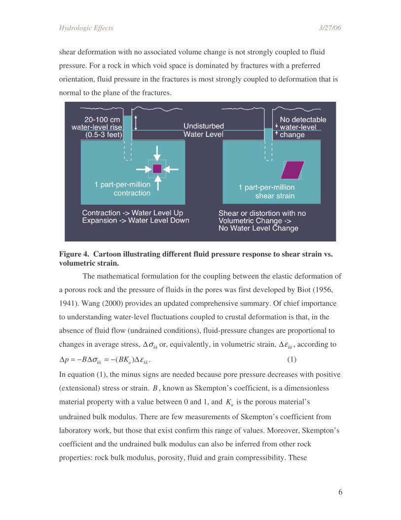
shear deformation with no associated volume change is not strongly coupled to fluid

pressure. For a rock in which void space is dominated by fractures with a preferred

orientation, fluid pressure in the fractures is most strongly coupled to deformation that is

normal to the plane of the fractures.

Figure 4. Cartoon illustrating different fluid pressure response to shear strain vs. volumetric strain.

The mathematical formulation for the coupling between the elastic deformation of

a porous rock and the pressure of fluids in the pores was first developed by Biot (1956,

1941). Wang (2000) provides an updated comprehensive summary. Of chief importance

to understanding water-level fluctuations coupled to crustal deformation is that, in the

absence of fluid flow (undrained conditions), fluid-pressure changes are proportional to

changes in average stress, ∆σkk or, equivalently, in volumetric strain, ∆εkk , according to

∆p = −B∆σkk = −(BKu )∆εkk . (1)

In equation (1), the minus signs are needed because pore pressure decreases with positive

(extensional) stress or strain. B , known as Skempton’s coefficient, is a dimensionless

material property with a value between 0 and 1, and Ku is the porous material’s

undrained bulk modulus. There are few measurements of Skempton’s coefficient from

laboratory work, but those that exist confirm this range of values. Moreover, Skempton’s

coefficient and the undrained bulk modulus can also be inferred from other rock

properties: rock bulk modulus, porosity, fluid and grain compressibility. These


7

calculations, observations of Earth tides in wells, and laboratory studies suggest that the

coefficient of proportionality between water-level changes and volumetric strain is in the

range of 30-100 cm/microstrain for rocks whose void space is in the form of pores. In a

homogeneous, isotropic rock no coupling is expected between shear strain and fluid

pressure.

In a rock where void space is dominated by fractures, the sensitivity of water

pressure to strain can be greater than in a porous rock, but is not as easily calculated

based on rock properties because the coefficient depends on fracture compliance. Bower

(1983) has shown how to relate fracture parameters to observed Earth tide response.

Observed coefficients of water-level change in response to strain in fracture-dominated

formations are as high as 2 m/microstrain (e.g., Woodcock and Roeloffs, 1996). Because

such formations are anisotropic, regional shear strain can in principle be coupled to local

fluid pressure variations.

If undrained conditions truly exist, then the fluid-saturated rock mass can simply

be thought of as an elastic material whose shear modulus is the same as that of the rock

itself, but with an “undrained” Poisson ratio, ν u , such that ν < ν u < 0.5 . There is no fluid

flow and no induced time-dependent strain.

3.3 Strain-fluid pressure coupling when conditions are not undrained

Subsurface fluid pressure varies in response to rainfall, pumping, or any other

factor changing the mass of fluid in the system. When fluid mass per unit volume of

material is not constant, equation (1) generalizes to

∆p = BKu −∆εkk +1

1− K / Ks

m − m0

ρ0

�

� � �

� � (2)

where K is the (drained) bulk modulus of the material, Ks is the bulk modulus of the

solid grains, and (m − m0 ) / ρ0 is the change in fluid mass per unit volume, divided by the

fluid density in a reference state. Equation (2) shows that fluid-mass changes are coupled

not only to fluid pressure changes, but also to volumetric strain changes.

3.4 Strainmeter signals produced by pore fluid pressure acting on the strainmeter


8

Segall et al. (2003) pointed out that increasing fluid pressure would apply

compressional stress to borehole strainmeters and produce contractional signals that do

not represent strain of the rock. Under isotropic conditions, the fluid pressure changes

would be expected to affect only areal or volumetric strain, not the shear strain. From

equation (14) of Segall et al. (2003), the ratio up /uε of instrument output in response to

fluid pressure change, to instrument output in response to volumetric strain of the rock, is

up /uε = 3(ν u −ν)(1+ α)2GB(1+ ν u)

(3)

where ν is the drained Poisson ratio, ν u is the undrained Poisson ratio, B is Skempton’s

coefficient, and G is the shear modulus (all for the rock in which the strainmeter is

installed), and α is the ratio of strainmeter output for a change in vertical strain to

strainmeter output for a change in radial strain. Note that α is not really known, but is

probably much smaller than 1 for a GTSM. An important fact about equation (3) is that it

predicts an apparent contractional strain signal in response to increasing fluid pressure.

This differs from the response of the crust itself in the absence of a strainmeter, for which

poroelastic coupling predicts extensional strain when fluid pressure rises. The reason is

that the strainmeter is an essentially impermeable inclusion. Table 1 lists some computed

values of up /uε for plausible values of ν , ν u , B, G, and α .

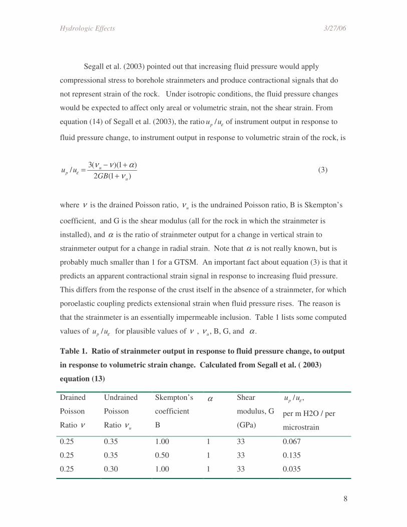
Table 1. Ratio of strainmeter output in response to fluid pressure change, to output

in response to volumetric strain change. Calculated from Segall et al. ( 2003)

equation (13)

Drained

Poisson

Ratio ν

Undrained

Poisson

Ratio ν u

Skempton’s

coefficient

B

α Shear

modulus, G

(GPa)

up /uε ,

per m H2O / per

microstrain

0.25 0.35 1.00 1 33 0.067

0.25 0.35 0.50 1 33 0.135

0.25 0.30 1.00 1 33 0.035


9

0.25 0.30 1.00 0 33 0.017

0.25 0.35 1.00 1 10 0.222

0.20 0.35 1.00 1 10 0.333

0.20 0.35 1.00 1 3 1.111

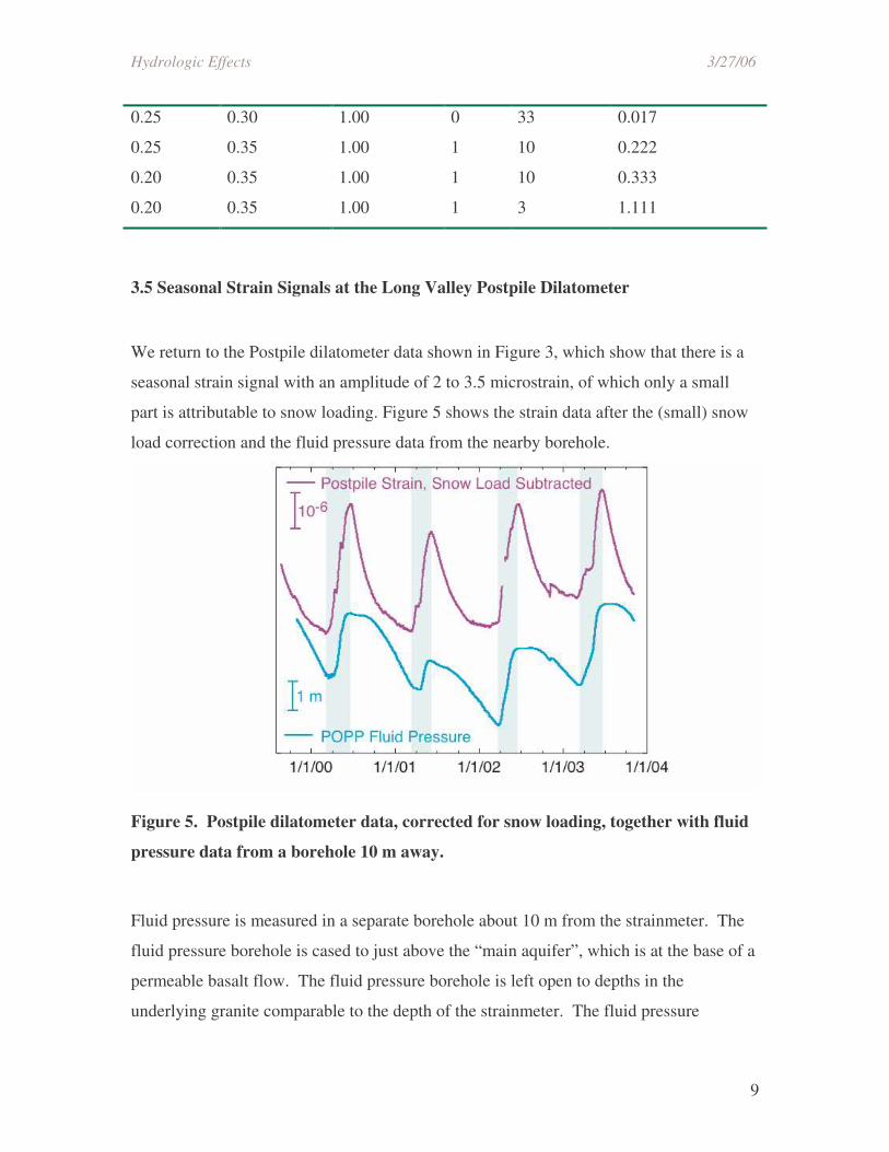
3.5 Seasonal Strain Signals at the Long Valley Postpile Dilatometer

We return to the Postpile dilatometer data shown in Figure 3, which show that there is a

seasonal strain signal with an amplitude of 2 to 3.5 microstrain, of which only a small

part is attributable to snow loading. Figure 5 shows the strain data after the (small) snow

load correction and the fluid pressure data from the nearby borehole.

Figure 5. Postpile dilatometer data, corrected for snow loading, together with fluid

pressure data from a borehole 10 m away.

Fluid pressure is measured in a separate borehole about 10 m from the strainmeter. The

fluid pressure borehole is cased to just above the “main aquifer”, which is at the base of a

permeable basalt flow. The fluid pressure borehole is left open to depths in the

underlying granite comparable to the depth of the strainmeter. The fluid pressure


10

measured with this configuration will be an average of the pressures in the permeable

aquifer and the granite.

In Figure 5, the periods of seasonal contractional strain are highlighted to show

that they correspond closely with the times when fluid pressure is increasing (which

coincide almost exactly with the times when snow is melting). Although the times of

peaks and troughs correspond, the actual time histories of fluid pressure and strain change

are somewhat different. However, comparing the net annual changes in strain and in

water level yields a ratio of strain change to fluid pressure change between 1 and 3

microstrain/m of water level change. The observed effect of the fluid pressure on the

strain data is consistent with the principle proposed by Segall et al. (2003), in that the

contractional strain coincides with increasing fluid pressure, consistent with the effect

being due to the pressure of the fluid acting on the relatively impermeable

strainmeter/grout inclusion. However, the ratio of observed strain to fluid pressure

change is at the high end of the values expected. A value as high as 1 microstrain/m of

water is obtained only for a low shear modulus (3 GPa) and a large difference between

ν and ν u (0.25 and 0.35, respectively).

Although the seasonal strain changes at the Postpile site are qualitatively

consistent with what’s expected from fluid pressure acting on the strainmeter, the fluid

pressure data at the Postpile site cannot be used with just a simple technique like linear

regression to correct the seasonal signal in the strain data. One possibility is that the fluid

pressure measurement made in a separate borehole, which is open not only to the granite

in which the strainmeter is installed, but also to a much more permeable formation, does

not track the fluid pressure in the immediate vicinity of the strainmeter. It is also possible

that the strainmeter experiences some degree of strain from deformation of the overlying

active aquifer as the pressure in that aquifer changes.

3.6 Seasonal Signals at Parkfield Donna Lee Site

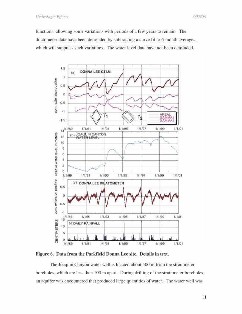
Figure 6 shows data from the Parkfield Donalee GTSM, Donalee dilatometer, and

Joaquin Canyon water well. The GTSM data are the areal and shear strains prepared by

CSIRO, which have been detrended by subtracting a combination of exponential


11

functions, allowing some variations with periods of a few years to remain. The

dilatometer data have been detrended by subtracting a curve fit to 6-month averages,

which will suppress such variations. The water level data have not been detrended.

Figure 6. Data from the Parkfield Donna Lee site. Details in text.

The Joaquin Canyon water well is located about 500 m from the strainmeter

boreholes, which are less than 100 m apart. During drilling of the strainmeter boreholes,

an aquifer was encountered that produced large quantities of water. The water well was


12

drilled through interbedded sand and clay, with a confining unit overlying a productive

aquifer about 152 m below the surface. The water well is open to the formation from 147-

153 m below the surface, so its water level is proportional to the pressure in this aquifer.

The dilatometer is at a depth of 176.5 m and the GTSM is at a depth of 174 m; both are

installed in sandstone. Although the depth at which the aquifer was encountered in the

strainmeter boreholes is not known, it is probably the same formation as that monitored

by the water well.

Variations with an approximately 1-year period are visible in all the strain data,

including the shear strains. Contractional strain coincides closely with increasing fluid

pressure for both the dilatometer and the GTSM areal strain, and maxima and minima of

γ 2 and γ1, respectively, coincide with peak extension. However, the amplitudes of the

seasonal cycles in the water level data vary much more than the amplitudes of the

seasonal strain cycles. The shear strain cycles approximately mirror each other and their

time histories closely resemble the time history of areal strain recorded by the GTSM.

The shapes of the annual cycles are distinctly different for the GTSM, water level, and

dilatometer. The areal and volumetric strain vary of the order of 0.5 microstrain/m of

water, comparable to the Postpile dilatometer, and at the high end of the range of

coefficients relating fluid pressure to strainmeter output (Table 1).

The seasonal variations in shear strain are about half as large as those in areal

strain, which is not expected in a model based on a uniform, isotropic porous elastic

medium. The poroelastic properties of Berea sandstone have been found to be anisotropic

(e.g., Lockner [2002]) in that properties measured in the direction perpendicular to

bedding differ from those measured parallel to bedding. However, anisotropy with

respect to the two bedding-parallel directions would seem to be required to induce shear

strain via a change in the fluid pressure in the formation surrounding the strainmeter.

Shear strain imposed by deformation of the aquifer itself seems a more likely

explanation.

The differences between the shapes of the seasonal strain cycles and the water

level cycles, the smaller year-to-year variability of the strain cycles, the large shear

strains, and the relatively large coefficient between fluid pressure change and areal and

vertical strain suggest that another mechanism may be operating. Temperature changes


13

induced by infiltration of precipitation are a candidate. The strainmeters are reputed to be

be extremely temperature sensitive, but the exact coefficient relating strainmeter output to

ambient temperature of the rock around the sensor is not known. Groundwater

temperature changes of 0.001-0.01ºC due to influx of meteoric water seem feasible and

should be evaluated as a contributing factor in seasonal strain variations.

4. Time-dependent drainage effects Undrained fluid-pressure changes in response to strain occur instantaneously with

deformation. In fact, the water-level variation would have the same time history as the

deformation were it not for the ability of water to flow. Flow causes spatial variations in

pressure to equilibrate with each other over a time scale governed by the material’s

hydraulic diffusivity. In particular, a sudden, localized change of pore pressure induced

by a tectonic event such as an earthquake or rapid intrusion will spread and dissipate with

time, causing time-dependent fluid pressure changes in locations not originally affected

by the tectonic event.

4.1 Vertical flow to the water table

The vertical flow path between the subsurface and the water table (sometimes

called “water table drainage”) can have a huge effect on fluid pressures that are induced

by strain, and, in principle, on data from borehole strainmeters. Here we will use

operational definitions of “water table” and “confined” aquifers specific to the purposes

of understanding their responses to strain. (We will also use the term “aquifer” for any

subsurface saturated formation, whereas hydrologists usually reserve the term for

formations that can supply useful quantities of water for human consumption.)

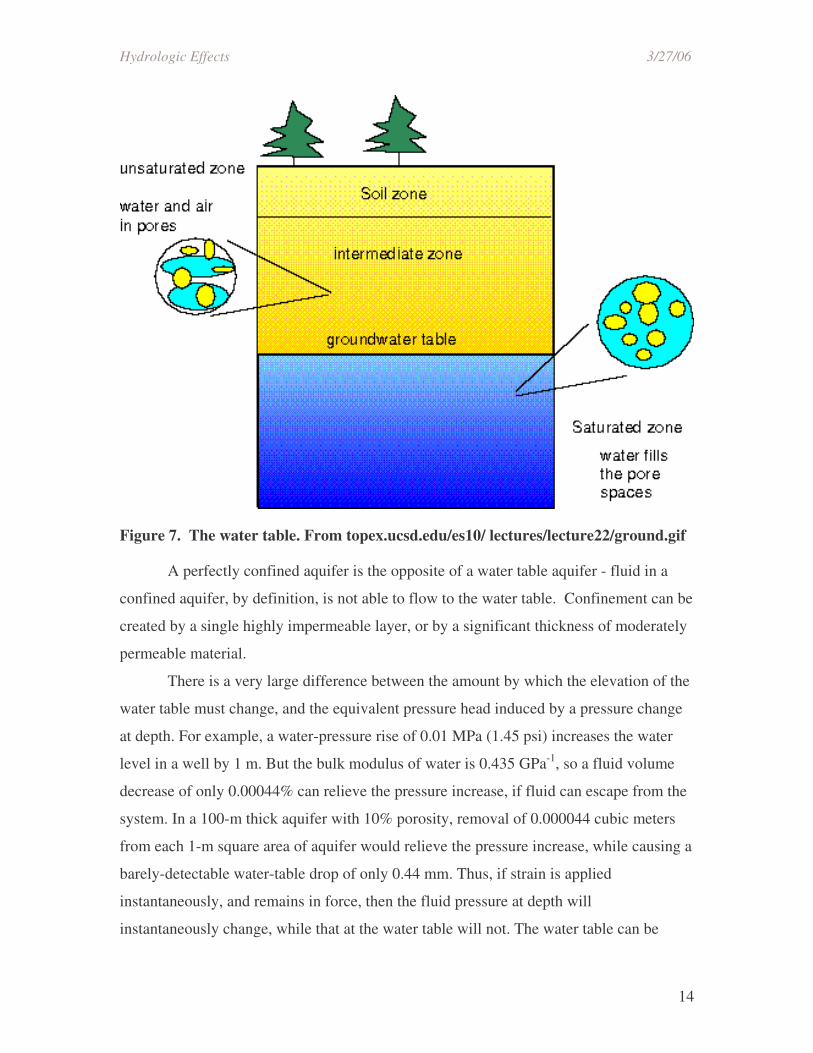
The water table is defined as the top of the zone of saturation. For our purposes,

the important thing about the water table is that there is empty pore space above it (Fig.

7). If rock at the depth of the water table is deformed, fluid in the pores has the option of

moving up or down into unoccupied pore space.


14

Figure 7. The water table. From topex.ucsd.edu/es10/ lectures/lecture22/ground.gif

A perfectly confined aquifer is the opposite of a water table aquifer - fluid in a

confined aquifer, by definition, is not able to flow to the water table. Confinement can be

created by a single highly impermeable layer, or by a significant thickness of moderately

permeable material.

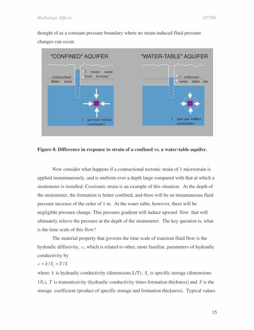
There is a very large difference between the amount by which the elevation of the

water table must change, and the equivalent pressure head induced by a pressure change

at depth. For example, a water-pressure rise of 0.01 MPa (1.45 psi) increases the water

level in a well by 1 m. But the bulk modulus of water is 0.435 GPa-1, so a fluid volume

decrease of only 0.00044% can relieve the pressure increase, if fluid can escape from the

system. In a 100-m thick aquifer with 10% porosity, removal of 0.000044 cubic meters

from each 1-m square area of aquifer would relieve the pressure increase, while causing a

barely-detectable water-table drop of only 0.44 mm. Thus, if strain is applied

instantaneously, and remains in force, then the fluid pressure at depth will

instantaneously change, while that at the water table will not. The water table can be


15

thought of as a constant-pressure boundary where no strain-induced fluid pressure

changes can occur.

Figure 8. Difference in response to strain of a confined vs. a water-table aquifer.

Now consider what happens if a contractional tectonic strain of 1 microstrain is

applied instantaneously, and is uniform over a depth large compared with that at which a

strainmeter is installed. Coseismic strain is an example of this situation. At the depth of

the strainmeter, the formation is better confined, and there will be an instantaneous fluid

pressure increase of the order of 1 m. At the water table, however, there will be

negligible pressure change. This pressure gradient will induce upward flow that will

ultimately relieve the pressure at the depth of the strainmeter. The key question is, what

is the time scale of this flow?

The material property that governs the time scale of transient fluid flow is the

hydraulic diffusivity, c , which is related to other, more familiar, parameters of hydraulic

conductivity by

c = k /Ss = T /S

where k is hydraulic conductivity (dimensions L/T), Ss is specific storage (dimensions

1/L), T is transmissivity (hydraulic conductivity times formation thickness) and S is the

storage coefficient (product of specific storage and formation thickness). Typical values


16

of specific storage range from about 10-7/m to 10-4/m. Note that although T and c have

the same dimensions, they have different physical meanings and their numerical values

differ by many orders of magnitude. The hydraulic conductivity is related to

permeability by:

(hydraulic conductivity)=

permeability*(fluid density)*(acceleration due to gravity)/(fluid viscosity)

Permeability is an intrinsic property of the rock; it has dimensions of L2, and is usually

expressed in darcies, with 1 darcy=10-12 m2. 1 darcy corresponds to a hydraulic

conductivity of approximately=10-5 m/s for water.

If the material between the depth, z , of the strainmeter and the depth, zw , of the

water table is assumed to have a uniform vertical hydraulic diffusivity, c , then the 1-D

diffusion equation for groundwater flow can be solved analytically to yield the time

history of pressure change, p(z, t) , caused by this vertical flow:

p(z, t) = −BKuε0erf {[(z − zw )2 /4ct]1/ 2} (4)

In equation (4), erf denotes the error function and ε0 denotes the amplitude of the

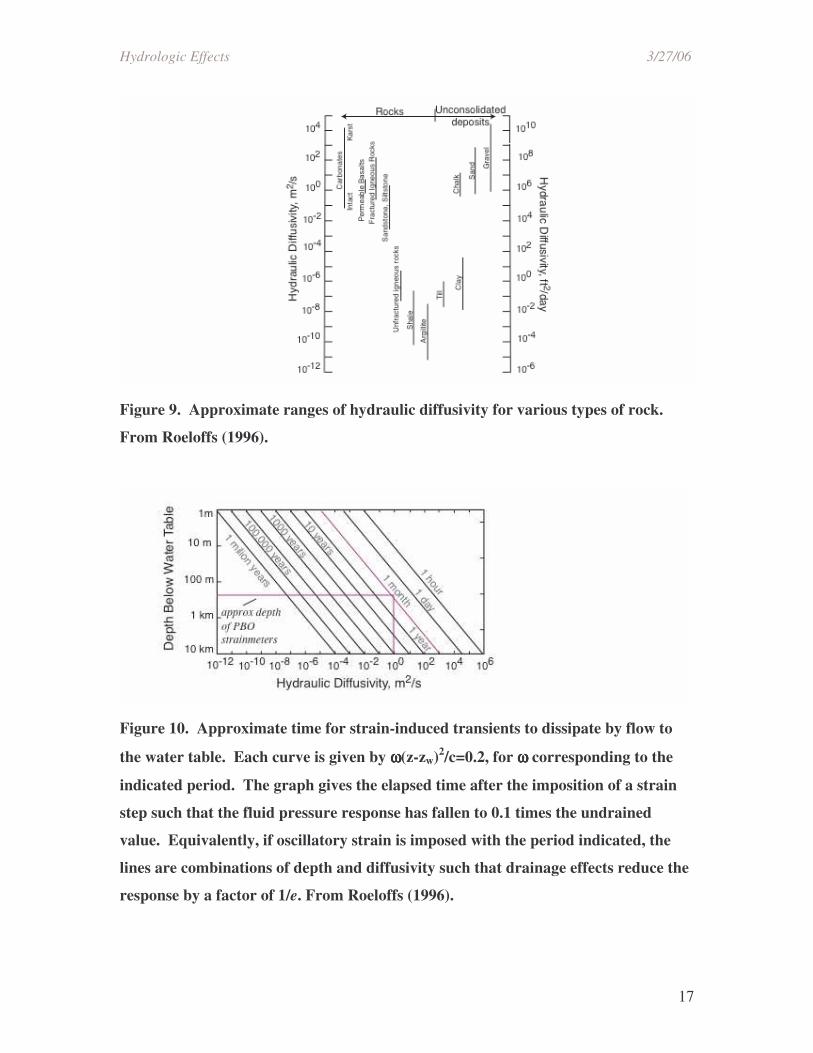
instantaneously applied strain (Roeloffs, 1996). Equation (4) implies that the time

required for strain-induced pressure to dissipate increases as the square of the depth

below the water table, and decreases in inverse proportion to the hydraulic diffusivity.

Since hydraulic diffusivity varies over many orders of magnitude (Figure 9), this time

scale also varies tremendously (Figure 10).


17

Figure 9. Approximate ranges of hydraulic diffusivity for various types of rock.

From Roeloffs (1996).

Figure 10. Approximate time for strain-induced transients to dissipate by flow to

the water table. Each curve is given by ωωωω(z-zw)2/c=0.2, for ωωωω corresponding to the

indicated period. The graph gives the elapsed time after the imposition of a strain

step such that the fluid pressure response has fallen to 0.1 times the undrained

value. Equivalently, if oscillatory strain is imposed with the period indicated, the

lines are combinations of depth and diffusivity such that drainage effects reduce the

response by a factor of 1/e. From Roeloffs (1996).


18

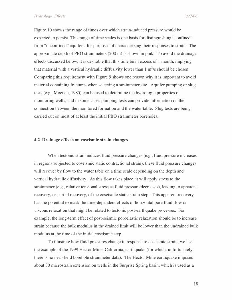
Figure 10 shows the range of times over which strain-induced pressure would be

expected to persist. This range of time scales is one basis for distinguishing “confined”

from “unconfined” aquifers, for purposes of characterizing their responses to strain. The

approximate depth of PBO strainmeters (200 m) is shown in pink. To avoid the drainage

effects discussed below, it is desirable that this time be in excess of 1 month, implying

that material with a vertical hydraulic diffusivity lower than 1 m2/s should be chosen.

Comparing this requirement with Figure 9 shows one reason why it is important to avoid

material containing fractures when selecting a strainmeter site. Aquifer pumping or slug

tests (e.g., Moench, 1985) can be used to determine the hydrologic properties of

monitoring wells, and in some cases pumping tests can provide information on the

connection between the monitored formation and the water table. Slug tests are being

carried out on most of at least the initial PBO strainmeter boreholes.

4.2 Drainage effects on coseismic strain changes

When tectonic strain induces fluid pressure changes (e.g., fluid pressure increases

in regions subjected to coseismic static contractional strain), these fluid pressure changes

will recover by flow to the water table on a time scale depending on the depth and

vertical hydraulic diffusivity. As this flow takes place, it will apply stress to the

strainmeter (e.g., relative tensional stress as fluid pressure decreases), leading to apparent

recovery, or partial recovery, of the coseismic static strain step. This apparent recovery

has the potential to mask the time-dependent effects of horizontal pore fluid flow or

viscous relaxation that might be related to tectonic post-earthquake processes. For

example, the long-term effect of post-seismic poroelastic relaxation should be to increase

strain because the bulk modulus in the drained limit will be lower than the undrained bulk

modulus at the time of the initial coseismic step.

To illustrate how fluid pressures change in response to coseismic strain, we use

the example of the 1999 Hector Mine, California, earthquake (for which, unfortunately,

there is no near-field borehole strainmeter data). The Hector Mine earthquake imposed

about 30 microstrain extension on wells in the Surprise Spring basin, which is used as a


19

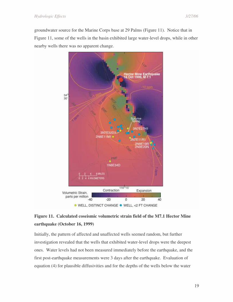
groundwater source for the Marine Corps base at 29 Palms (Figure 11). Notice that in

Figure 11, some of the wells in the basin exhibited large water-level drops, while in other

nearby wells there was no apparent change.

Figure 11. Calculated coseismic volumetric strain field of the M7.1 Hector Mine

earthquake (October 16, 1999)

Initially, the pattern of affected and unaffected wells seemed random, but further

investigation revealed that the wells that exhibited water-level drops were the deepest

ones. Water levels had not been measured immediately before the earthquake, and the

first post-earthquake measurements were 3 days after the earthquake. Evaluation of

equation (4) for plausible diffusivities and for the depths of the wells below the water


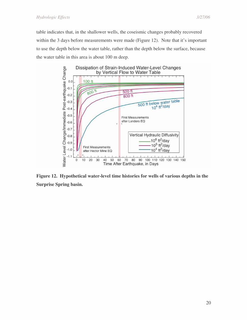
20

table indicates that, in the shallower wells, the coseismic changes probably recovered

within the 3 days before measurements were made (Figure 12). Note that it’s important

to use the depth below the water table, rather than the depth below the surface, because

the water table in this area is about 100 m deep.

Figure 12. Hypothetical water-level time histories for wells of various depths in the

Surprise Spring basin.


21

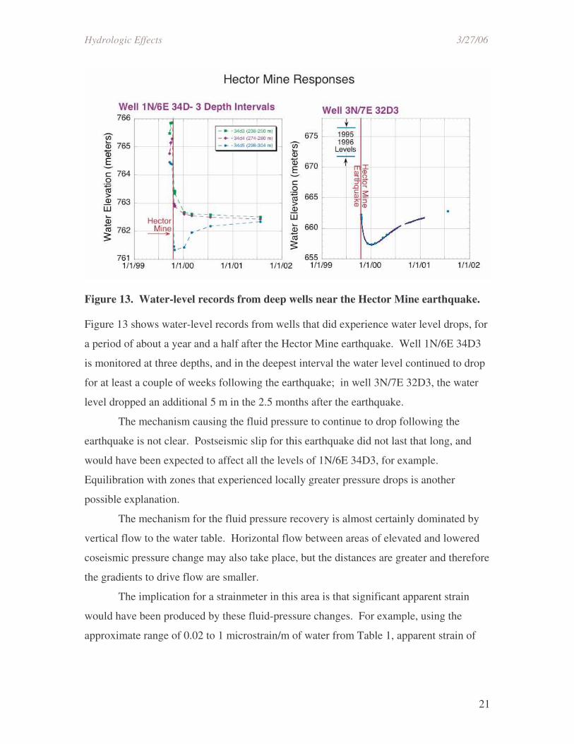
Figure 13. Water-level records from deep wells near the Hector Mine earthquake.

Figure 13 shows water-level records from wells that did experience water level drops, for

a period of about a year and a half after the Hector Mine earthquake. Well 1N/6E 34D3

is monitored at three depths, and in the deepest interval the water level continued to drop

for at least a couple of weeks following the earthquake; in well 3N/7E 32D3, the water

level dropped an additional 5 m in the 2.5 months after the earthquake.

The mechanism causing the fluid pressure to continue to drop following the

earthquake is not clear. Postseismic slip for this earthquake did not last that long, and

would have been expected to affect all the levels of 1N/6E 34D3, for example.

Equilibration with zones that experienced locally greater pressure drops is another

possible explanation.

The mechanism for the fluid pressure recovery is almost certainly dominated by

vertical flow to the water table. Horizontal flow between areas of elevated and lowered

coseismic pressure change may also take place, but the distances are greater and therefore

the gradients to drive flow are smaller.

The implication for a strainmeter in this area is that significant apparent strain

would have been produced by these fluid-pressure changes. For example, using the

approximate range of 0.02 to 1 microstrain/m of water from Table 1, apparent strain of


22

0.1 to 5 microstrain could have been caused by the continuing 5 m of water-level drop at

well 3N/7E 32D3.

4.3 Possible apparent strain from anomalous post-earthquake fluid pressure

changes

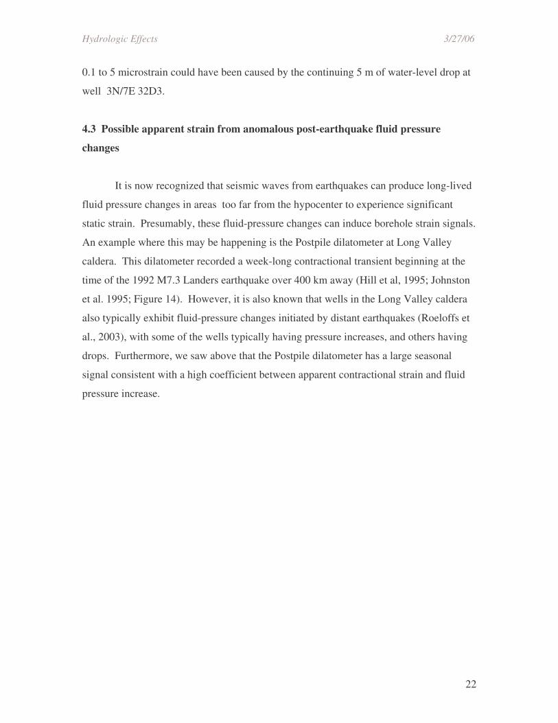
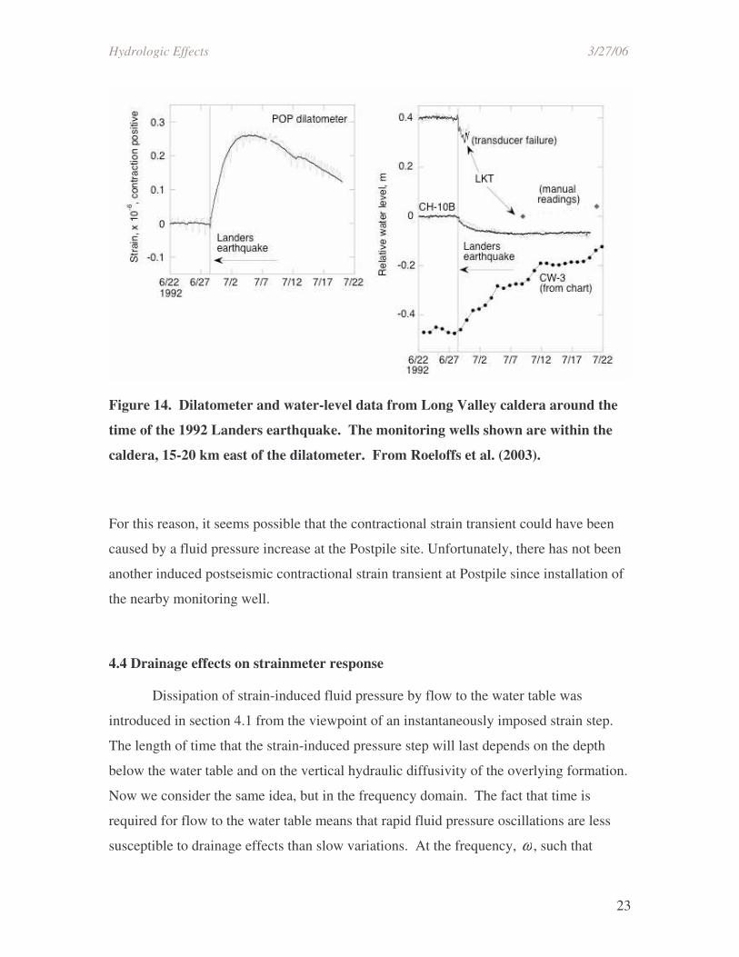
It is now recognized that seismic waves from earthquakes can produce long-lived

fluid pressure changes in areas too far from the hypocenter to experience significant

static strain. Presumably, these fluid-pressure changes can induce borehole strain signals.

An example where this may be happening is the Postpile dilatometer at Long Valley

caldera. This dilatometer recorded a week-long contractional transient beginning at the

time of the 1992 M7.3 Landers earthquake over 400 km away (Hill et al, 1995; Johnston

et al. 1995; Figure 14). However, it is also known that wells in the Long Valley caldera

also typically exhibit fluid-pressure changes initiated by distant earthquakes (Roeloffs et

al., 2003), with some of the wells typically having pressure increases, and others having

drops. Furthermore, we saw above that the Postpile dilatometer has a large seasonal

signal consistent with a high coefficient between apparent contractional strain and fluid

pressure increase.


23

Figure 14. Dilatometer and water-level data from Long Valley caldera around the

time of the 1992 Landers earthquake. The monitoring wells shown are within the

caldera, 15-20 km east of the dilatometer. From Roeloffs et al. (2003).

For this reason, it seems possible that the contractional strain transient could have been

caused by a fluid pressure increase at the Postpile site. Unfortunately, there has not been

another induced postseismic contractional strain transient at Postpile since installation of

the nearby monitoring well.

4.4 Drainage effects on strainmeter response

Dissipation of strain-induced fluid pressure by flow to the water table was

introduced in section 4.1 from the viewpoint of an instantaneously imposed strain step.

The length of time that the strain-induced pressure step will last depends on the depth

below the water table and on the vertical hydraulic diffusivity of the overlying formation.

Now we consider the same idea, but in the frequency domain. The fact that time is

required for flow to the water table means that rapid fluid pressure oscillations are less

susceptible to drainage effects than slow variations. At the frequency, ω , such that


24

ω(z − zw )2 /c = 0.2, drainage reduces the amplitude of the pressure oscillation by a factor

of 1/e times the undrained response. Periods much shorter than this are not affected by

drainage, but longer periods will be increasingly affected. Figure 10 can also be used to

visualize this period as a function of depth and diffusivity. Comparing Figures 9 and 10

shows that for vertical diffusivities at the upper end of the expected range for fractured

igneous rocks, drainage at a depth of 200 m may influence signals with periods of days.

When a strainmeter is subjected to strain at a period long enough for drainage to

occur, its apparent sensitivity to strain will be lower than at undrained periods. An

undrained contractional strain is accompanied by elevated fluid pressure that acts to

further compress the strainmeter. When drainage occurs, this elevated fluid pressure is

not there, so the strainmeter experiences less compression, even though the strain of the

rock is the same. Under these conditions, the strainmeter will have a frequency response

whose gain drops with increasing period. We saw in an earlier chapter that the frequency

response of a dilatometer can be estimated by calculating its cross-spectrum with

atmospheric pressure, and that at least two California dilatometers (Vineyard Canyon and

Sunol) have frequency response that decreases at periods of days.

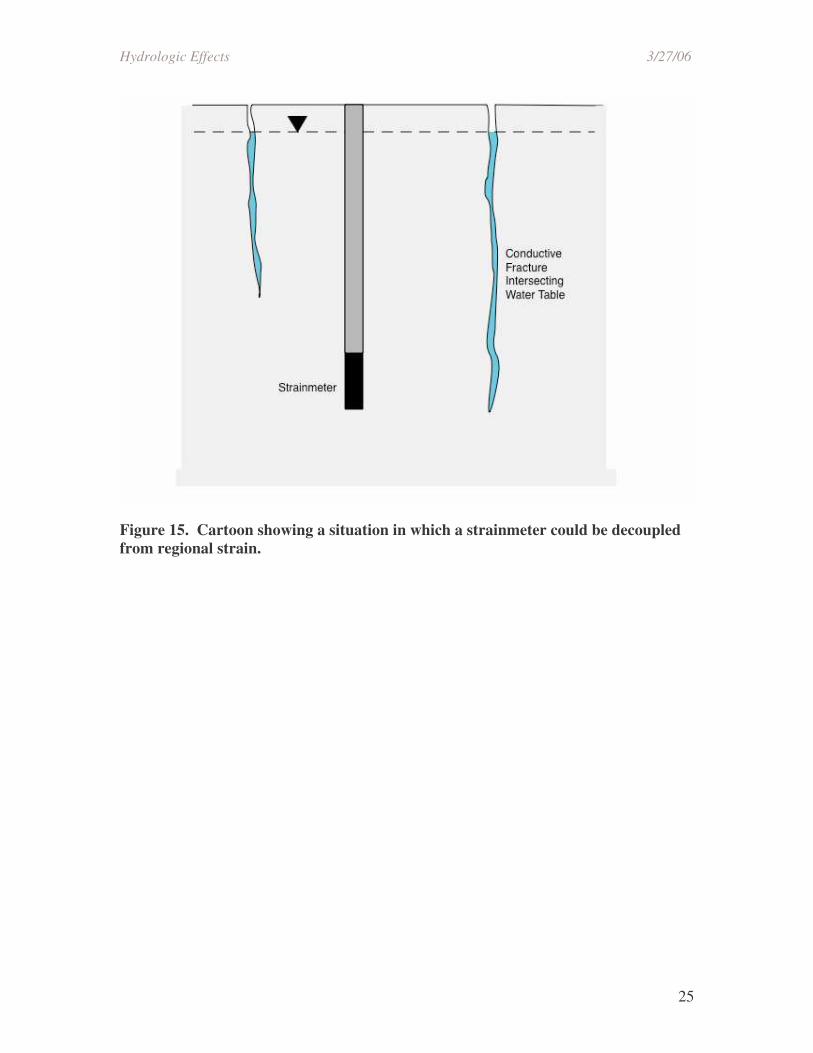
Jonsson et al. (2003) have raised the possibility that a borehole strainmeter could

be installed in a location that is essentially decoupled from crustal strain on a scale of

more than a few meters from the borehole. This situation requires not only that drainage

occur at periods of days or less, but also that almost all strain be accommodated by

deformation of pore space or fractures. The concern is motivated by the behavior of the

BUR dilatometer in Iceland, for which the responses to two different earthquakes and

two different volcanic eruptions have been essentially the same, after scaling by the

maximum magnitude, and consist of a rapid step followed by a decay over 3-4 days. The

long-term record of data from this instrument shows negligible long-term strain. A

preliminary analysis of the atmospheric pressure response of the instrument shows that its

response to atmospheric pressure fluctuations falls off at long periods, with a noticeable

effect at periods of several days.


25

Figure 15. Cartoon showing a situation in which a strainmeter could be decoupled from regional strain.


26

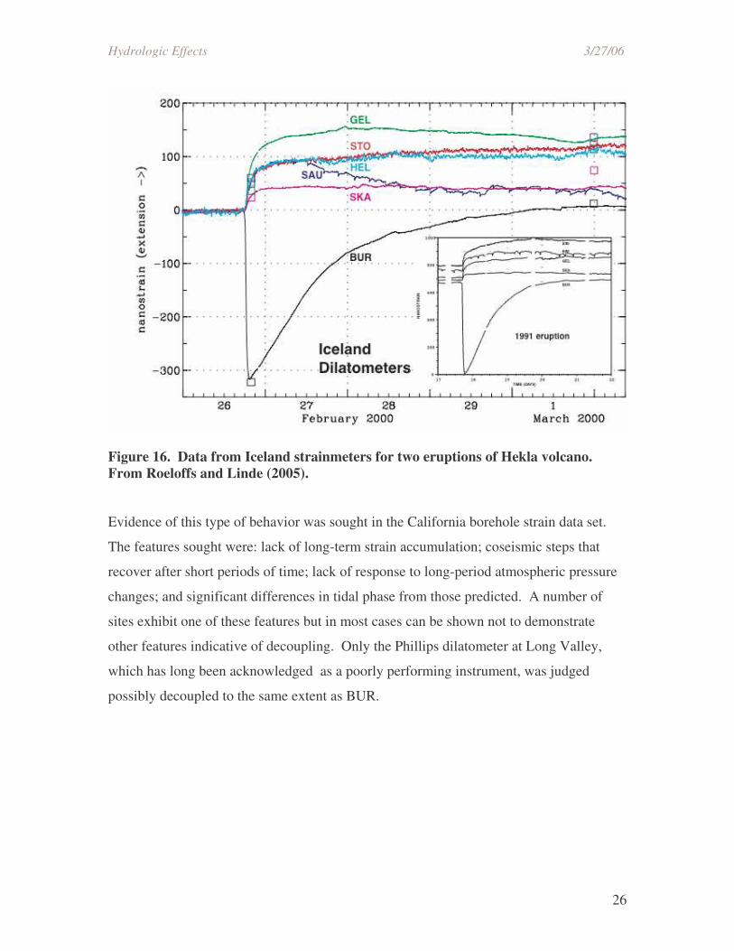
Figure 16. Data from Iceland strainmeters for two eruptions of Hekla volcano. From Roeloffs and Linde (2005).

Evidence of this type of behavior was sought in the California borehole strain data set.

The features sought were: lack of long-term strain accumulation; coseismic steps that

recover after short periods of time; lack of response to long-period atmospheric pressure

changes; and significant differences in tidal phase from those predicted. A number of

sites exhibit one of these features but in most cases can be shown not to demonstrate

other features indicative of decoupling. Only the Phillips dilatometer at Long Valley,

which has long been acknowledged as a poorly performing instrument, was judged

possibly decoupled to the same extent as BUR.


27

References cited

Biot, M.A., General theory of three-dimensional consolidation, Jour. Appl. Phys., 12, 155-164, 1941. Biot, M.A., General solutions of the equations of elasticity and consolidation for a porous material, Jour. Appl. Mech., 91-96, 1956. Bower, D.R., Bedrock fracture parameters from the interpretation of well tides, J. Geophys. Res., 88 (B6), 5025-5035, 1983. Hill, D.P., M.J.S. Johnston, J.O. Langbein, and R. Bilham, Response of Long Valley Caldera to the Mw 7.3 Landers, California, earthquake, Journal of Geophysical Research, 100 (B7), 12,985-13,005, 1995. Johnston, M.J.S., D.P. Hill, A.T. Linde, J. Langbein, and R. Bilham, Transient deformation during triggered seismicity from the 28 June 1992 Mw=7.3 Landers earthquake at Long Valley Volcanic Caldera, California, Bull. Seismol. Soc. Am., 85 (3), 787-795, 1995. Jonsson S, Segall P, Agustsson K, Agnew D. Local fluid flow and borehole strain in the South Iceland Seismic Zone. Eos Trans. AGU, 84 (46), Fall Meet. Suppl., Abstract G31B-0717, 2003 Lockner, D.A., S.A. Stanchits, Undrained poroelastic response of sandstones to a deviatoric stress change, J. Geophys. Res., 107 (B12), 2353 doi:10.1029/2001JB001460, 2002. Moench, A.F., Transient flow to a large-diameter well in an aquifer with storative semi-confining layers, Water Resour. Res., 21, 1121-1131, 1985. Roeloffs, E.A., Poroelastic techniques in the study of earthquake-related hydrologic phenomena, Advances in Geophysics, 37, 135-195, 1996. Roeloffs, E., M. Sneed, D.L. Galloway, M.L. Sorey, C.D. Farrar, J.F. Howle, J. Hughes, Water level changes induced by local and distant earthquakes at Long Valley caldera, California, J. Volc. Geotherm. Res., 127, 269-303, 2003. Roeloffs E, Linde AT. Borehole observations of continuous strain and fluid pressure. In Volcano Geodesy, D. Dzurisin, in press, 2005. Segall, P., S. Jónsson, K. Agustsson, When is the strain in the meter the same as the strain in the rock?, Geophys. Res. Letters, v. 30, no 19, doi:10.1029/2003GL017995, 2003. Wang, H.F., Theory of linear poroelasticity with applications to geomechanics and hydrogeology, 287 pp., Princeton University Press, 2000.


28

Woodcock, D., and E. Roeloffs, Seismically-induced water level oscillations in a fractured-rock aquifer well near Grants Pass, Oregon, Oregon Geology, 58 (2), 27-33, 1996.

Online Resource

California Data Exchange Center

-snowpack, rainfall, temperature, and streamflow data for California

http://cdec.water.ca.gov/

coupling of hydrologic effects to borehole strain data · coupling of hydrologic effects to...

Documents