couples’ migration and marital instability ying li
TRANSCRIPT

COUPLES’ MIGRATION AND MARITAL INSTABILITY
by
YING LI
B.A., China Agricultural University, 2005
M.A., University of Colorado at Boulder, 2007
A thesis submitted to the
Faculty of the Graduate School of the
University of Colorado in partial fulfillment
of the requirement for the degree of
Doctor of Philosophy
Department of Economics
2011

This thesis entitled:
Couples’ Migration and Marital Instability
written by Ying Li
has been approved for the Department of Economics
Terra McKinnish
Jeffrey Zax
Date
The final copy of this thesis has been examined by the signatories, and we
Find that both the content and the form meet acceptable presentation standards
Of scholarly work in the above mentioned discipline.
IRB protocol # ____0509.3_____________

iii
Ying Li (Ph.D., Economics)
Couples’ Migration and Marital Instability
Thesis directed by Associate Professor Terra McKinnish
Full-time working couples are more likely to face the co-location issue than other couples. Co-
location conflicts could affect migration decisions, labor market choices, and ultimately, marital
stability. This dissertation studies how occupation mobility (or occupation migration rate) affects
these outcomes for full-time working couples in the United States.
Having some probability of relocating one's job in the future can create a locational conflict
between spouses if the other spouse is also working and has his/her own preferred job location. If
this locational conflict is not fully expected before marriage, joint location becomes less possible
and marital stability is endangered. In this study I use occupation mobility as the proxy for the
uncertainty of future occupation migration. Occupation mobility is measured as the fraction of
workers in an occupation who have moved across state lines during the five years prior to the
year of U.S. Census report. The dissertation consists of three parts: a study on migration and
earning outcomes using cross-sectional data from the 5% Public-Use Microdata Samples
(PUMS) of Census 2000, an analysis of marital status based on the same data from Census 2000,
and a study on marital stability using data from the National Longitudinal Survey of Youth 1979
and three rounds of Census: 1980, 1990 and 2000.

Dedicated to my parents and my husband

v
ACKNOWLEDGMENTS
First and foremost, I would like to express my deepest appreciation to my advisor,
Professor Terra McKinnish, for all the time, energy, and encouragement given to me throughout
this dissertation. Her openness in sharing her knowledge and insight has given me the tools to
pursue the high professional standards and academic excellence that she has attained.
I would like to also thank my committee members: Professors Jeffrey Zax, Francisca
Antman, Jonathan Hughes and Laura Argys, for valuable discussions and suggestions that help
improve this dissertation.

vi
CONTENTS
INTRODUCTION ..........................................................................................................................1
CHAPTER ONE .............................................................................................................................4
1.1 Introduction .....................................................................................................................4
1.2 Literature Review ............................................................................................................6
1.3 Data and Sample .............................................................................................................9
1.4 Empirical Analysis ........................................................................................................22
1.5 Results ...........................................................................................................................24
1.6 Conclusion ....................................................................................................................28
CHAPTER TWO ..........................................................................................................................29
2.1 Introduction ...................................................................................................................29
2.2 Literature Review ..........................................................................................................31
2.3 Empirical Analysis and Results Using Census Data .....................................................36
CHAPTER THREE ......................................................................................................................46
3.1 Empirical Analysis Using NLSY79 Data .....................................................................46
3.2 Results of NLSY79 .......................................................................................................59
3.3 Conclusion ....................................................................................................................66
BIBLIOGRAPHY .........................................................................................................................68

vii
TABLES
Table
1. 1.1 Most Common Occupations for Power Couples ......................................................13
1.2 Distribution of Occupation Motilities of Career people ...........................................15
2. 2.1 Conditional Frequency Distributions for Individuals
by Education Category and by Occupation Category ...............................................17
2.2 Conditional Frequency Distributions for Couples
by Education Category and by Occupation Category ...............................................18
3. Occupation Characteristics ............................................................................................19
4. Descriptive Statistics ......................................................................................................21
5. Results of Equation 1 .....................................................................................................25
6. Results of Equation 2 .....................................................................................................27
7. Descriptive Statistics, Census 2000 ...............................................................................37
8. Estimates of Probability of Divorce Status ....................................................................41
9. Estimates of Linear Probability of Divorce Status ........................................................43
10. The Effects of Mobility on Divorce Status, Fixed Effect Model ...................................45
11. Descriptive Statistics for Variables in Cross-section Regressions ................................49
12. Relationship between Pre-marriage and Post-marriage Migration ................................56
13. 13-1 OLS Estimation of Probability of Divorce (Occupation) ......................................60
13-2 OLS Estimation of Probability of Divorce
(Industry-Occupation) .............................................................................................60
14. OLS Estimation of Probability of Divorce Controlling for
Pre-marriage Migration ..................................................................................................62
15. OLS Estimation of Probability of Divorce Controlling for
Most Recent Pre-marriage Migration ............................................................................65

viii
16. Discrete Divorce Hazard Model .....................................................................................66

1
Introduction
Chapter 1
This chapter extends recent literature on power-couple migration. Power couples are referred
to as couples in which both spouses have at least a college degree. Some of these couples may
not experience conflicts over re-location. The reason is if one party in the marriage is not
pursuing a career, this party is more likely to yield the choice of location to that of the spouse. As
a result, previous studies on power-couple migration may reduce to studies on power individual
migration. This finding motivates our work on career-couple migration. If both spouses work in a
career occupation, they form a career couple. Career occupation is defined as an occupation in
which the percentage of workers with at least a college degree is relatively large and earnings
growth of a typical worker is comparatively high. Couples in which both members work in a
career occupation should be more likely to experience conflict over re-location decisions.
Following McKinnish (2008), we examine the effects of occupation-education mobility. The
sample in this analysis is from the 5% PUMS of Census 2000. Using a binary logit model, the
migration study shows that male occupation-education mobility has a positive and considerably
larger effect on the family migration than that of women. The earnings analysis provides some
evidence of positive selective matching from career wives to career husbands. This finding is
hard to reconcile with complementarity, the theoretical prediction by Becker (1973).

2
Chapter 2
Prospective migration of one party or both parties in a marriage can lead to the locational
conflict between the two spouses. Mincer (1978) suggests that this discord can result in marital
instability. We use occupational mobility as a proxy for prospective migration to test for an effect
on ever-married persons’ marital status. By Mincer’s hypothesis, all else being equal, a person
working in an occupation with higher mobility is more likely to face conflicts on optimal
location choices with the working spouse, and their marriage is thus more likely to break up.
Using linear probability models and data from the 5% PUMS of Census 2000, basic analysis
shows that higher occupational mobility predicts a larger probability of divorce status for all
education/gender groups except for the college educated male. This effect is higher among
non-college-educated people than among their college-educated counterparts for both genders.
But the effect declines substantially when occupational mobility is replaced by
occupation-industry mobility, controlling for occupation and industry fixed effects.
Chapter 3
Although 5% PUMS of Census 2000 has the benefit of a very large sample size, it does not
allow one to distinguish first marriage from re-marriage. In contrast, data from the National
Longitudinal Survey of Youth 79 (NLSY79) make this distinction possible. NLSY79 also has
rich information on marriage histories, spouse’s occupation and individual characteristics, and
the Geocode data also contain information such on location and migration. In the final chapter,
we use these data to test the relationship between occupation mobility and divorce.

3
A main concern on the measure of occupational mobility is that, it may in part reflect one’s
taste for migration, meaning that people who like to move choose highly mobile occupations.
The correlation can confound the true effect of occupational mobility, the proxy for prospective
migration, on marital stability. This potential endogeneity is discussed and partially addressed in
the current chapter. Using the Geocode data, one’s pre-marital migration history is constructed
and controlled as a proxy for individuals’ preference for migration.
Using both linear probability model and logit discrete time hazard model, we do not find
sufficient evidence to support that occupation mobility affects the stability of first marriages.
Rational expectation of future occupation migration before marriage or a unitary approach on
family migration is offered to explain these findings.
4
Chapter One
1.1 Introduction
Recent research on migration focuses on couples or households who may or may not act as a
single decision maker. Following the study by Costa and Kahn (2000), much attention is placed
on the migration behavior of power couples, formed by spouses who both own at least a college
degree. It is documented that among married couples, the proportion of power couples in the
United States rose from 2 percent in 1940, to 9 percent in 1970, and further to 15 percent in 1990.
The location choices of power couples are worth studying for at least two important reasons. First,
while geographic locations are crucial for the career of a highly educated person, the influx and
exodus of many highly educated people may have a long-term effect on the development of cities.
Second, though these ―dual-career‖ couples are very likely to experience within household
trade-off or bargaining on the optimal assignment of their co-locations, less has been known
concerning the socio-economic consequences of migration.
The classification of couples based on their education level, however, simply overlooks two
facts: there is great heterogeneity in occupation mobility for highly educated workers, and many
of them may not really work for an occupation with opportunities for career advancement and
salary growth. Statistics has shown us that a fairly large fraction of husbands and wives holding
college or even graduate degrees are in occupations without much potential for a career. For
example, among power couples, 18.6% wives and 5.6 % husbands are elementary and middles

5
school teachers, according to 2000 Decennial Census.1 Although a couple formed by two highly
educated spouses is powerful in terms of education, it is possible that one spouse, say the wife,
does not pursue career in her occupation and thus yields her own location to the husband’s optimal
location. If this is the case, previous studies on power couples’ migration may reduce to studies on
a power individual’s migration.
Unlike the existing literature on couples’ migration which often classifies couples based on
education, this paper takes a different step by dividing occupations into career occupations and
non-career occupations. A career occupation should satisfy two requirements: the percentage of
workers with at least a college degree is relatively large and the earnings growth of a typical
worker is comparatively high. We then reclassify couples into four groups: dual-career couples,
husband-only career couples, wife-only career couples and non-career couples.
In the regression analysis, we replicate McKinnish (2008) by investigating how occupational
attributes such as mobility and occupation wage rate affect household location choices as well as
earnings of spouses. Occupation-education mobility is measured by the proportion of workers in
an occupation-education class who have moved across state lines in the past five years. 2
Empirical results also show that occupation-education mobility for both husband and wife has a
positive effect on a family’s migration decision for all couple groups, with the effect by the
1 Elementary and middle teachers are not a career occupation based on the concept defined in this paper.
2 This follows the definition of mobility by McKinnish (2008).

6
husband’s occupation-education mobility being considerably larger. Meanwhile, the earnings
analysis implies a positive selective matching story for career wives. This seems not to be
reconciled with the well-established theory by Becker (1973) that very career-oriented men will
seek less career-oriented women so that wives will devote energy to their husband’s career.
The rest of this chapter is organized as follows. The next section provides a literature review.
Section 1.3 discusses data and samples used in the regressions, which is followed by a detailed
description on how to define career occupations. Empirical strategies are specified in Section 1.4.
Results are reported in Section 1.5. The last section 1.6 concludes.
1.2 Literature Review
Migration is defined by the Population Association of America as a ―relatively permanent
change of residence that crosses jurisdictional boundaries (counties in particular), measured in
term of usual residence at a prior point in time, typically 1-5 years earlier. Local moves within
jurisdictions are preferably defined as residential mobility.‖ The key distinction between
migration and residential mobility is that the former involves a move to a new labor market and
the latter does not. This paper focuses on migration across state lines.
In the neoclassical unitary model, a family will migrate if migration improves (expected)
household income more than migration cost. A husband or wife can become a ―tied-mover‖ or
―tied-stayer‖ if their individual losses are smaller than their partner’s gains [Sandell 1977; Mincer

7
1978]. The bulk of the empirical evidence suggests that migrating wives experience more
negative labor market outcomes than migrating husbands [Boyle et al. 2001; Boyle et al. 2002;
Cooke 2003; Nivalainen 2004; Cooke and Speirs 2005; Astrom and Westerlund 2006; Shauman
and Noonan 2007].3
Most early empirical studies on household migration do not allow the effects to vary by
education level, yet the existing evidence points to the opposite. Greenwood (1975 and 1993)
establishes that the propensity to migrate decreases with age and increases with education. The
migration pattern and its subsequent outcomes could be different with respect to different
education levels. Basker (working paper 2003) models a previously unexamined relationship
between education and the purpose of migration: the high educated tends to move with jobs at
hand while the low educated is more likely to move for jobs searching. He then verifies this
theoretical prediction using CPS data. In other words, migration behavior differs across education
groups.
More recent literature investigates the location decisions of highly-educated couples. Estimates
using samples from the integrated public use census (Ruggles and Sobeck 1997) show that
college educated couples are increasingly located in large metropolitan areas. These areas are
home to 32 percent of all college educated couples in 1940, 39 percent by 1970, and 50 percent
3 Boyle et al. (2002) use British vs. U.S. data; Nivalainen (2004) uses Finnish data; Astrom and Westerlund (2006)
use Swedish data; Others use U.S. data.
8
by 1990. Costa and Kahn (2000) argue that ―power couples‖, in which both spouses have at least
a college degree, increasingly move to large cities where both parties can more easily find jobs
suitable for their careers. Using census data, Costa and Kahn (2000) find that the co-location
hypothesis explains 65 percent of the increased concentration of power couples in large
metropolitan areas. Compton and Pollak (2007) find some evidence that contradicts the findings
by Costa and Kahn using data from the Panel Study of Income Dynamics (PSID). Specifically,
they show that couples with a college educated husband and a non-college educated wife are as
likely to migrate to large city areas as power couples. They also demonstrate that the observed
locational trends of power couples are better explained by higher rates of power couples
formation rather than migration to large metropolitan areas.
McKinnish (2008) also studies migration of highly-educated couples. Using the 2000
Decennial Census, McKinnish calculates migration rates by occupation and education groups. She
then estimates the effects of these occupation mobility measures on migration decisions and labor
market outcomes of married couples. Her results show that compared with the wife’s occupation
mobility, the husband’s occupation mobility has a much larger positive effect on household
migration. Among never-married individuals with college degrees however, men and women’
migration behavior equally responds to their respective occupation mobility. For couples in which
the husband has a college degree, regardless of wife’s education, wife’s occupation mobility has a
positive effect on husband’s earnings, whereas husband’s occupation mobility has a larger but
significantly negative effect on wife’s earnings. Such effects are considerably weaker among

9
couples in which only the wife has a college degree. These findings may suggest that a more
mobile wife is generally helpful in the location choices of the husband, while a more mobile
husband tends to exert unfavorable influence on the migration decisions of the wife.
Costa and Kahn (2000), Compton and Pollak (2007) and McKinnish (2008) all study
college-educated couples under the assumption that these couples are more likely to encounter the
problem of balancing two careers when making joint location decisions. As we argue below,
however, lots of college-educated workers have jobs with little potential for career advancement.
We thus re-examine the results by Costa and Kahn (2000) and by McKinnish (2008), by
classifying couples based on their occupation and education rather than simply on their education.
1.3 Data and Sample
1.3.1 Census Data
This paper uses the 5% Public Use Microdata Sample (PUMS) from the 2000 Decennial
Census. Occupation is reported for the worker’s current job, and for a non-worker, the most
recent job in the past 5 years. Workers are classified into 504 civilian occupation categories.
An important assumption in our analysis is that workers’ occupation classifications are
relatively stable over time. That is, although migration involves one’s move to a new labor
market, the majority of migrants are still employed in their pre-migration occupations. The latest
findings on occupation stability are mixed. Moscarini and Thomsson (2007) use monthly CPS to

10
show that between 1979-2006, 3.5% of male workers employed in two consecutive months
report changes in occupation; while using PSID, Kambourov and Manovskii (2008) find that in
the year of 1997, average annual occupation change rate is 15% at the one-digit occupation level,
17% at the two-digit level, and 20% at the three-digit level.4 In addition, their results indicate
that for each age group, more educated people (some college and college) experienced both a
lower level and a smaller increase in their occupation change rates than less educated people
(high school and less). Therefore, our assumption on occupational stability better applies to the
group of highly educated workers. Sullivan (2010) finds from NLSY79 that, at three-digit
occupation level, the yearly across firm occupation switch is between 20% and 30% from 1980
to 1990, and is less than 20% from 1990 to 2000. Also, the fraction of employed individuals
reporting within-firm occupation switch averages at 21% between the 1980 and 1993 survey
years, peaks in 1993 at 25%, and declines to be 7% in 2000. In general, there is a decreasing
trend of occupation change rate according to NLSY79.5
The analysis in this paper makes use of two samples: a large sample used to calculate
occupation characteristics and a small regression sample. The large sample includes all workers
with age between 25 and 55 (the period in which career is more likely to motivate migration)
4 Kambourov and Manovskii (2008) find that average annual occupation change rate has increased from 10% to 15%
at the one-digit occupation codes, from 12% to 17% at the two-digit level, and from 16% to 20% at the three-digit
level during the period of 1968-1997. 5 The data of occupation change in Sullivan (2010) is obtained by aggregating the weekly NLSY employment
data into a yearly employment record. Even though NLSY becomes biennial interviews after 1994 instead of annual
interviews, consistent weekly labor force records make the occupation change comparable before and after 1994. In
chapter 3, the analysis of the effect of occupation mobility on marital instability is based on NLSY79.

11
who resided in the U.S. in 1995 and for whom occupation, education and migration status are not
allocated. These workers are sorted using by 504 occupations and 8 education classifications:
less than 9th
grade, some high school, high school diploma, some college education, bachelor’s
degree, master’s degree, professional degree, and doctoral degree. This large sample is then used
to calculate the migration rate and average wage of each occupation-education category. The
mobility measure is the fraction of workers in that occupation-education class who have
migrated across state lines in the past 5 years. Average wages are computed only for workers
with a reported wage between $3 per hour and $300 per hour. The regression sample consists of
workers in the large sample who are non-Hispanic white and dual-earner married couples with
age between 25 and 55. 6
1.3.2 Career Occupations
Previous papers often categorize couples based on their education. The implicit assumption is
that college-educated workers are more likely to pursue careers for which location is a crucial
factor in career advancement. Nonetheless, it is also observed that many college educated workers
have jobs with little scope for career advancement. For example, 18.6% of working wives in
power couples are elementary or middle-school teachers. In other words, it doesn’t make much
sense to define power couples based only on one’s education and then to study how these
―dual-career‖ couples solve their co-location problems when facing migration decisions. We
6 Some recent works such as Astrom and Westerlund (2006) and Compton and Pollak (2007) also include
co-habitants as couples. This paper only examines legally married couples.

12
believe that it is imperative to redefine couples in terms of career occupations and this should
improve our understanding of real dual-career couples’ migration decisions and their
post-migration earnings. In the regressions, couples are divided into four groups: both spouses in
career occupations (career couples), only husband in a career occupation (husband career couples),
only wife in a career occupation (wife career couples), and neither in a career occupation
(non-career couples).
In this paper a career occupation has to satisfy these two conditions: 1) the percentage of
college graduates in an occupation is at least one standard deviation above the mean of the
percentage of college graduates among all occupations, 2) its earnings gap (90 percentile - 50
percentile) is above the median of earnings gap in all occupations. These two criteria are
designed to determine which occupations require a high skill level and have the potential for
high (cross sectional) earnings growth. The remaining occupations are called non-career
occupations.
According to Census 2000, there are 30.7% full time workers having at least a college degree.
Using 5% PUMS, I calculate the mean and standard deviation for percentage of college educated
workers by occupations, which are 26% and 28% respectively; the median of earnings gap in all
occupations is $25,000. Therefore, by our approach, an occupation is a career occupation if at
least 54% of its workers are college graduates and its earnings gap is at least $25,000.

13
Table 1-1 lists 30 most common occupations for power couples. These occupations are
provided in the first column, followed by two columns for the number of male and female
observations in the regression sample. The last two columns report the percentage of college
graduates and earnings gap (using the large sample) for each occupation. Observe that only 13
out of these 30 occupations are career occupations (highlighted in bold letters). Also note that in
the regression sample, only 17% of power couples are career couples.
Table 1-1 Most Common Occupations for Power Couples
Occupations Number
of men
Number
of Women
Percent of
College
Graduate
Earning
Gap
Elementary and Middle School Teachers 7,445 24,971 83.52% 23,000
Registered Nurses 719 8,717 50.38% 25,000
Accountants and Auditors 4,276 4,602 67,23% 40,000
Secondary School Teachers 3,887 4,872 94.18% 24,000
Postsecondary Teachers 3,871 4,003 88.08% 45,000
Managers, All Other 4,957 2,372 45.60% 40,500
Lawyers 4,817 2,510 99.73% 110,000
Marketing and Sales Managers 3,384 2,576 63.16% 61,000
Education Administrator 3,070 2,758 73.16% 39,000
Chief Executives 4,046 945 58.66% 247,000
Sales Representatives, Wholesale and
Manufacturing
3,613 1,284 36.87% 55,500
Financial Managers 3.022 1,744 52.05% 61,500
Physicians and Surgeons 2,603 1,596 99.49% 241,000
First-Line Supervisors/Managers of Retail
Sales Workers
2,418 1,132 19.57% 38,000
General and Operations Managers 2,603 867 43.74% 62,000
Secretaries and Administrative Assistants 216 3,178 12.32% 18,000

14
Notes: Power couples are the couples in which both spouses have at least a college degree.
Career couples are the couples in which both spouses are in career occupations. An Occupation
is a career occupation if at least 54% of its workers are college graduates and its earnings gap is
at least $25,000. The bolded occupations are career occupations.
Table 1-2 provides the distribution of occupation-education mobility of career people with
college degree by female and by male. Average occupation-education mobility is 0.164.
Generally, the occupations with more involvement of local network are the ones having relative
lower mobility.
Computer Software Engineers 2,427 917 74.98% 42,000
Retail Salespersons 1,651 1,683 13.91% 32,000
Human Resources, Training, and Labor
Relations Specialists
1,074 2,152 43.44% 36,800
Counselors 1,058 2,114 65,67% 26,000
First-Line Supervisors/Managers of Office
and Administrative Support Workers
1,366 1,793 28.12% 27,000
Social Workers 772 2,374 71.36% 19,500
Computer Scientists and Systems
Analysts
1,709 928 57.22% 41,000
Management Analysts 1,559 1,027 72.02% 74,000
Clergy 2,012 429 72.77% 26,000
First-Line Supervisors/Managers of
Non-Retail Sales Workers
1,737 691 31.20% 60,700
Computer Programmers 1,618 744 59.82% 36,700
Customer Service Representatives 832 1,239 15.62% 21,400
Sales Representatives, Services, All Other 1,372 652 36.41% 60,000
Preschool and Kindergarten Teachers 28 1,929 36.04% 18,500

15
Table 1-2 Distribution of Occupation Motilities of Career people
Female
High Mobility Occupations Mobility
Materials Engineers 0.5135
Industrial Engineers, Including Health and Safety 0.43103
Market and Survey Researchers 0.39772
Dietitians and Nutritionists 0.37931
Agricultural and Food Scientists 0.36904
Low Mobility Occupations Mobility
Dentists 0.0873
Librarians 0.0772
Education Administrator 0.08047
Legislators 0.05714
Judges, Magistrates, and Other Judicial Workers 0.0292
Male
High Mobility Occupations Mobility
Materials Engineers 0.51351
Budget Analysts 0.5
Industrial Engineers, Including Health and Safety 0.43103
Financial Analysts 0.37837

16
Agricultural and Food Scientists 0.369047
Low Mobility Occupations Mobility
Legislators 0.05714
Surveyors, Cartographers, and Photogrammetrists 0.0476
Electrical and Electronics Engineers 0.0392
Judges, Magistrates, and Other Judicial Workers 0.0292
Mechanical Engineers 0.0285
Notes: This sample includes college graduated career people (married individuals in career
occupations) from Census 2000 PUMS. Mobility is occupation-education mobility, measured by
the fraction of workers in certain occupation-education category who ever moved across state
line in the past five years.
1.3.3 Descriptive Statistics
Table 2-1 presents the conditional frequency distributions for individuals by education
category and by occupation category (male and female separately). The top numbers in each row
sum to one, so do the bottom numbers in each column. For example, 43% of college educated
men are in career occupations; while 79% of men in career occupations have at least a college
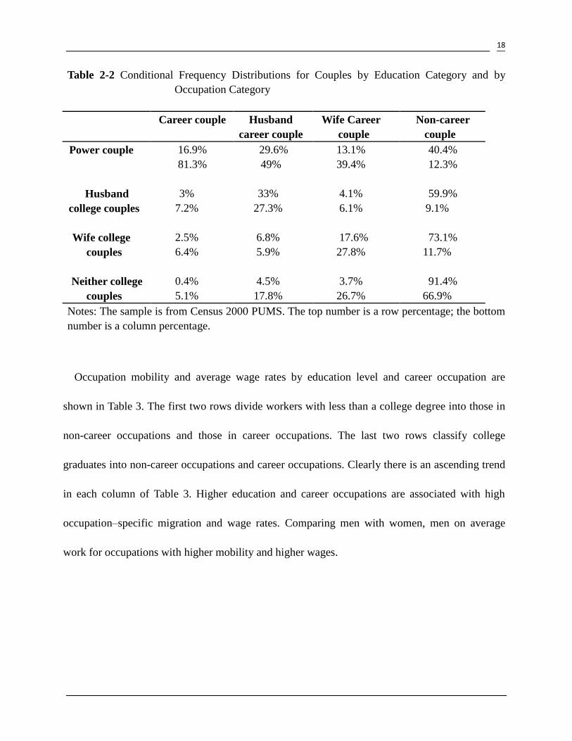
degree. Table 2-2 provides the conditional frequency distributions for couples grouped by
education and for couples grouped by occupation. In each cell, the top number is the proportion
of couples by the education group that are also couples by the corresponding occupation group,
and vice versa for the bottom number. For instance, only a small proportion of power couples
(16.9%) are career couples, while most of career couples (81.3%) are power couples. It is also

17
interesting to see that almost ¾ of husband career couples are not husband college couples ,
which can largely be explained by the fact that a half (49%) of husband career couples are power
couples. There is a similar pattern for wife career couples, with about two fifths of them being
power couples.
Table 2-1 Conditional Frequency Distributions for Individuals by Education Category and by
Occupation Category
Men Career Non-career
College degree or
higher male
43% 57%
79% 24%
Less than College
degree
5.7% 94.3%
21% 76%
Women Career Non-career
College degree or
higher female
27% 73%
75% 29%
Less than College
Degree
4.6% 95.3%
25% 71%
18
Table 2-2 Conditional Frequency Distributions for Couples by Education Category and by
Occupation Category
Career couple Husband
career couple
Wife Career
couple
Non-career
couple
Power couple 16.9% 29.6% 13.1% 40.4%
81.3% 49% 39.4% 12.3%
Husband
college couples
3% 33% 4.1% 59.9%
7.2% 27.3% 6.1% 9.1%
Wife college
couples
2.5% 6.8% 17.6% 73.1%
6.4% 5.9% 27.8% 11.7%
Neither college
couples
0.4% 4.5% 3.7% 91.4%
5.1% 17.8% 26.7% 66.9%
Notes: The sample is from Census 2000 PUMS. The top number is a row percentage; the bottom
number is a column percentage.
Occupation mobility and average wage rates by education level and career occupation are
shown in Table 3. The first two rows divide workers with less than a college degree into those in
non-career occupations and those in career occupations. The last two rows classify college
graduates into non-career occupations and career occupations. Clearly there is an ascending trend
in each column of Table 3. Higher education and career occupations are associated with high
occupation–specific migration and wage rates. Comparing men with women, men on average
work for occupations with higher mobility and higher wages.

19
Table 3 Occupation Characteristics
Occupation-Education
Specific Migration Rate
Occupation-Education
Specific Average wage
Men Women Men Women
Less than college degree in
non-career occupation
0.069
(0.024)
0.072
(0.023)
16.85
(3.14)
14.38
(3.24)
Less than college degree in
career occupation
0.102
(0.030)
0.092
(0.027)
25.05
(6.07)
21.06
(5.79)
College degree or more in
non-career occupation
0.125
(0.044)
0.110
(0.040)
24.98
(6.38)
21.74
(5.28)
College degree or more in
career occupation
0.167
(0.056)
0.157
(0.054)
32.90
(10.99)
28.87
(9.69)
Notes: This sample includes white, non-Hispanic, native-born, co-working couples from 2000
Census PUMS with both partners ages 25-55. Occupation-Education Specific Migration Rate is
measured by the fraction the workers in certain occupation-education class who have migrated
across the state line the past 5 years. Occupation-Education Specific Average wage is computed
for workers with reported wage between $3 per hour and $300 per hour in certain
occupation-education category.
Sample means of key variables used in the regression analysis are presented in Table 4.
Columns 1,3,5,7 are for couples grouped by occupation. In Columns 2,4,6,8, the same data are
used but couples are grouped by education. In order to show the differences between our approach
of grouping couples by occupation and the previous one by education, we treat power couples as
counterparts of career couples, husband college couples as counterparts of husband career couples,
and so on. Compared with spouses in power couples, those in career couples tend to have higher
individual earnings, higher occupation-education migration rates and average wages, and higher
education level. In addition, though there are nearly as many wife college couples as husband

20
college couples, husband career couples are twice as many as wife career couples. This implies
that many highly educated wives are not working in career occupations.
For married couples, we also pay attention to how spouses match one another with respect to
occupation. The theory of marriage (Becker 1973) predicts negative assortative mating in wage
rates. For example, high wage men tend to marry low-wage women who spend more time in
household production, rather than in labor markets. But spouses are positively matched in traits
such as physical capital, education and height. Empirical evidence also shows that the
resemblance of spouses has been increasing. Schwartz and Mare (2005) show that educational
homogamy in prevailing marriages has been rising from 1960 to 2003, which can partly be
attributed to a higher increase in educational attainment for women than for men.
The descriptive statistics in Table 4 seems to provide some evidence of positive assortative
matching in the occupation classification. To see this, first look at wife career couples and wife
college couples. It is obvious that husbands’ occupation-education migration rate, average wage
rate and average education level are on average higher in wife career couples. Similar patterns can
be found for wives, by comparing husband career couples with husband college couples. For
instance, wives’ average occupation-education migration rate is higher by 0.021, average
occupation wage rate is higher by 3.3 and average educational level is higher by 0.86 in husband
career occupations. In sum, statistics indicate that workers in career occupations are more likely to
have spouses who also make higher earnings, receive more education and of course are more

21
mobile.
Table 4 Descriptive Statistic
1 2 3 4 5 6 7 8
Career
couple
Power
couple
Husband
career
Husband
college
Wife
Career
Wife
College
Non
Career
Neither
college
Cross-State Migration
in Past 5 years 0.156 0.117
0.119
0.087 0.100 0.062 0.066 0.049
Husband’s Earnings 83,185
(72,233)
70,693
(61,887)
73,585
(61,548)
62,389
(49,162)
52,027
(44,667)
43,800
(32,310)
42,976
(31,188)
39,660
(5,736)
Wife’s Earnings 52,078
(50,321)
40,109
(37,421)
29,618
(27754)
24,810
(22,403)
42,300
(36057)
35,078
(25,193)
24,622
(19,833)
21,929
(16,985)
Husband’s
Occupation-Education
Migration Rate
0.165
(.06)
0.147
(0.056)
0.150
(.0569)
0.138
(0.050)
0.101
(.047)
0.078
(0.029)
0.08
(.037)
0.070
(0.025)
Wife’s
Occupation-Education
Migration Rate
0.155
(.059)
0.126
(0.051)
0.097
(.0392)
0.078
(0.024)
0.131
(.053)
0.116
(0.043)
0.08
(.032)
0.073
(0.024)
Husband’s
Occupation-Education
Average Wage
32.91
( 10.93)
29.05
(9.82)
30.74
(10.50)
27.07
(8.74)
21.38
( 6.70)
18.30
(4.23)
18.51
(5.16)
17.11
(3.76)
Wife’s
Occupation-Education
Average Wage
29.257
(10.395)
24.27
(7.89)
19.012
(5.881)
15.68
(4.06)
25.474
(8.573)
22.45
(6.33)
16.04
(4.88)
14.49
(3.56)
Husband’s Education 5.736
(1.181)
5.59
(0.84)
5.254
(1.141)
5.32
(0.64)
4.386
(1.083)
3.66
(0.55)
3.756
(1.046)
3.29
(0.75)
Wife’s Education 5.626
(1.123)
5.48
(0.71)
4.604
(.980)
3.74
(0.48)
4.976
(1.096)
5.31
(0.58)
3.886
(1.009)
3.38
(0.68)
Husband’s Age 41.078
(7.999)
41.15
(8.35)
42.309
(8.007)
43.44
(7.70)
40.699
(7.976)
40.21
(7.92)
41.339
(7.899)
41.36
(7.73)
Wife’s Age 39.492
(7.759)
39.62
(8.20)
40.702
(7.919)
41.44
(7.67)
38.969
(7.741)
38.59
(7.77)
39.577
(7.794)
39.58
(7.64)
Any Children under
18 0.597 0.607 0.606 0.592 0.593 0.623 0.620 0.623
Any Children under 6 0.306 0.286 0.229 0.198 0.285 0.300 0.230 0.213
N 27,938 134,151 81,024 66,934 44,621 70,240 439,578 321,614

22
Notes: The sample in Table 4 is the same as in Table 3. Columns 1,3,5,7 are for couples grouped
by occupation: career couples (both are in career occupation), only the husband is in a career
occupation, only the wife is in a career occupation, neither is in a career occupation. Columns
2,4,6,8 are the couples grouped by education: power couples (both have a college degree), only
the husband has a college degree, only the wife has a college degree, neither has a college
degree.
1.4 Empirical Analysis
This section of the paper replicates the analysis in McKinnish (2008). The major difference is
that couples are grouped based on occupation rather than on education. The empirical analysis
includes two parts: household migration decisions and the effect of spousal occupational
characteristics on own earnings. In the regressions, couples are divided into four groups: career
couples, husband career couples, wife career couples and non-career couples.
1.4.1 Migration Decisions
We estimate the effect of occupation mobility on married couple’s migration decisions using
the following Logit model:
log [ 𝑃𝑟𝑜𝑏( 𝑌𝑐ℎ𝑤𝑠 = 1)/𝑃𝑟𝑜𝑏(𝑌𝑐ℎ𝑤𝑠 = 0)] =
∝0+∝1 𝑀𝑐ℎ +∝2 𝑀𝑐𝑤 +∝3 𝑊𝑎𝑔𝑒𝑐ℎ + ∝4 𝑊𝑎𝑔𝑒𝑐𝑤 + 𝑋𝑐𝜃 + 𝑆𝑡𝑎𝑡𝑒𝑐𝑠𝛿 + 𝑆𝑡𝑎𝑡𝑒𝑐𝑠 ∗
𝑈𝑟𝑏𝑎𝑛𝑐𝛾 (1)
Where Y is an indicator variable for cross-state migration between 1995 and 2000 for couple c
with husband’s occupation class h and wife’s occupation class w living in state s. On the right

23
hand side, M is the occupation mobility; Wage is logarithm of average wage in an occupation; X
is a vector of demographic controls for both husband and wife, including age, age squared, a
dummy of presence of children under 18, a dummy of presence of children under 6, education
level. Also, we include state fixed effect and the interaction between state and urban residence,
controlling for the heterogeneities across states and the differences between urban area and
non-urban area in the same state. The average marginal effects of one’s own and the spouse’s
occupation mobility are expected to be positive and asymmetric.
1.4.2 Earnings Analysis
We estimate an earnings regression of the form:
𝐸𝑎𝑟𝑛𝑖𝑜𝑝𝑠 = 𝛽0 + 𝛽1𝑀𝑖𝑜 + 𝛽2𝑀𝑖𝑝 + 𝛽3𝑊𝑎𝑔𝑒io + 𝛽4𝑊𝑎𝑔𝑒i𝑝 + 𝑋𝑖𝜃 + 𝑂𝑐𝑐𝑖𝑜𝜙 + 𝑆𝑡𝑎𝑡𝑒𝑖𝑠𝛿 +
𝑆𝑡𝑎𝑡𝑒𝑖𝑠 ∗ 𝑈𝑟𝑏𝑎𝑛𝑖𝛾 + 휀𝑖𝑜𝑝𝑠 (2)
Where the dependent variable, 𝐸𝑎𝑟𝑛𝑖𝑜𝑝𝑠, is the logarithm of annual earnings in 1999 for person
i in occupation o with the spouse being in occupation p living in state s. The independent
variables are similar to those in equation 1, except that 𝑂𝑐𝑐𝑖𝑜 controls one’s own occupation
fixed effect. The primary interest is the effect of spouse’s occupation mobility.
One may argue that the assortative matching based on unobserved factors can bias the effect of
spousal occupation mobility on own earnings. For example, a man in a mobile career occupation

24
tends to seek his wife in a less mobile non-career occupation so that she can devote more time to
their household. However, assume that this assortative mating occurs largely based on
occupation, then controlling for one’s occupation fixed effect already significantly reduces the
concern on this endogeneity issue.7 It is also possible that some people get married before
choosing their occupations. In such cases, we have to worry about the occupation assignment (or
division) issue within a family. But the data in 2000 Census do not allow us to check this
possibility.
1.5 Results
1.5.1 Migration Results
Table 5 reports the average marginal effects of mobility and wage rates for four career
occupation categories using Equation 1. The corresponding effects under education classification
from McKinnish (2008) are also reported.8 Average marginal effects of husband’s and wife’s
occupation-education migration rate are given in the first two rows. Both husband’s and wife’s
occupation-education migration rate positively affects a family’s migration probability for all
couple groups, with the effect of the husband’s occupation mobility considerably larger. For
career couples, the effect of husband’s occupation mobility is higher in magnitude than those for
7 Following the seminal work by Becker (1973, 1974), there has been a huge literature in economics on matching in
the marriage market. Typically, empirical studies focus on matching based on one’s education, income, beauty,
attractiveness and socioeconomic background. To the best of our knowledge, there are no papers studying spousal
matching in terms of occupation.
8 Note that these results don’t match those of McKinnish (2008) because of cross-state migration is replaced by
cross –MSA migration in her final version.

25
power couples (0.690 vs. 0.602), and the effect of husband’s occupation mobility in non-career
couples is lower than that in neither college couples (0.486 vs. 0.543). Moreover, the gap between
the effect of the husband’s occupation mobility and that of the wife’s occupation mobility
increases for career couples and husband career couples, but decreases for wife career couples and
non-career couples.9 This result implies that in the decision of family migration, occupation
mobility of career husbands matters more than that of career wives.
Table 5 Results of Equation 1
Career
Couple
Power
Couple
Husband
Career
Husband
College
Wife
Career
Wife
College
Non
Career
Neither
College
Husband’s Occupation
–education Migration
Rate
0.690
(0.03)
0.602
(0.021)
0.64
(0.021)
0.585
(0.023)
0.576
(0.04)
0.636
(0.026)
0.486
(0.011)
0.543
(0.016)
Wife’s Occupation –
education Migration
Rate
0.385
(.039)
0.387
(0.032)
0.425
(.03)
0.459
(0.072)
0.272
(.03)
0.310
(0.030)
0.333
(.011)
0.362
(0.030)
Husband’s Occupation
Education Average
Wage
-0.008
(.007)
-0.0043
(0.0034)
-.012
(.004)
0.0011
(0.0037)
-0.024
(.006)
-0.0002
(0.004)
-0.0008
(.001)
0.0045
(.0019)
Wife’s
Occupation-education
Average Wage
-0.017
(.008)
-0.022
(.0050)
-0.007
(.005)
-0.029
(0.0050)
-0.001
(.005)
0.0003
(0.004)
0.0018
(.002)
-0.001
(0.0025)
N 27,915 134,151 81,002 66,932 44,531 70,240 439,489 321,614
Notes: Table 5 reports average marginal effects of occupation-education mobility from Equation
(1). Columns 1,3,5,7 are for couples grouped by occupation and Columns 2,4,6,8 are the couples
grouped by education as in Table 4. Occupation-education mobility is an occupation characteristic
measured by the fraction of workers who moved across state line in the past five years in certain
9 Standard errors are calculated by delta method.

26
occupation-education category. In this logit model, the dependent variable is an indicator for
cross-state migration between 1995 and 2000. This model includes controls for the husband’s age
and age squared, wife’s age and age squared, presence of children under 18, presence of children
under 6, indicators for husband’s and wife’s education level (less than high school, some high
school, some college, college degree, bachelor’s degree, master’s degree, professional degree, and
doctoral degree), state fixed effect and interaction between state and state and urban residence.
Standard errors for average marginal effects are calculated by delta method.
1.5.2 Earnings Analysis
The first column of Table 6 reports the effects of spouse’s occupation mobility from
Equation 2, while the second column reports the effects of spouse’s occupation mobility from
McKinnish (2008) by education category. For couples in which the husband is
college-educated, regardless of wife’s education, wife’s occupation mobility has a positive
effect on husband’s earnings, but husband’s occupation mobility has an even larger,
significantly negative impact on wife’s earnings. Clearly, the negative effects of husband’s
occupation mobility on wives’ earnings are smaller in career couples compared with power
couples. Since 75% career wives have at least a college degree while only 27% college
graduated wives are in career occupations, the wives in career couples are those with
relatively high wage and education and they are less likely to receive negative impact from
the husbands. Also, wives in wife career couples are more negatively affected by their
husbands, in comparison with wives in wife college couples. This can be explained by
positive assortative matching as well: because a husband who marries a career wife tends to
be competent himself, and thus is more likely to exert negative influence on his wife. Finally,
for husband career couples, the gap of the spousal effects widens, which implies a pattern of

27
negative assortative matching. Overall, compared with college educated wives, career wives
are more likely to match with relatively able husbands; whereas compared with college
educated husbands, career husbands do not necessarily seek out highly competent wives.
Table 6 Results of Equation 2
Effects of Spouses’ mobility
Occupation Category Education Category
Career couple Power couple
Husband 0.058
(0.076)
0.117
(0.072)
Wife -.603
(0.092)
-.869
(0.156)
N 27,917 120,726
Husband Career Husband college
Husband .476
(.061 )
0.397
(0.276)
Wife -.974
(.055)
-0.795
(0.201)
N 81,072 60,154
Wife Career Wife college
Husband -0.136
(0.064)
0.026
(0.073)
Wife -0.302
(.092)
-0.156
(0.158)
N 44,470 63,117
Neither Career Neither College
Husband -0.111
(0.029)
-0.491
(0.183)
Wife -0.25
(0.034)
-0.055
(0.144)
N 439,473 289,398
Notes: The sample includes white, non-Hispanic, native-born, co-working couples from 2000

28
Census PUMS with both partners ages 25-55. Dependent variable is the logarithm of own annual
earnings in 1999. The first column reports estimates of β2 from equation (2), which is the
coefficient on the migration rate in the spouse’s occupation-education group, while the second
column reports the effects of spouse’s occupation mobility from McKinnish (2008) by education
category. Regressions include same controls listed in notes of Table 5, with the addition of
occupation fixed-effects.
1.6 Conclusion
This paper discusses the migration behavior of couples who are classified according to career
occupations. Our approach to studying couples is better than the previous approach in terms of
capturing the joint migration decisions of couples with dual-career desire. Empirical results show
that both husband’s and wife’s occupation-education mobility positively affect the likelihood of a
family’s migration in each couple group, with the effect from the husband’s side being dominant.
More importantly, earnings analysis provides certain evidence of positive assortative matching
for career wives, which is not predicted by Becker’s (1973) theory.
Since we group couples based on occupation, a possible extension in the future is to examine
the effects of other occupation attributes. Also, unobserved time-invariant individual
characteristics, say migration preferences, that are correlated with occupation mobility cannot be
controlled for using Census data. One way to correct this omitted variable bias is to employ
panel data.
29
Chapter Two
2.1 Introduction
In his well-known paper, Mincer (1978; p.769) points out, ―As I argued in the theoretical
discussion, conflicting private locational incentives cannot always be reconciled, and prospective
or actual migration may lead to family dissolution.‖ To the best of our knowledge, this
hypothesis has not been tested. For researchers who may intend to estimate the true marital effect
of actual migration, the major obstacle is the endogeneity of actual migration choices. Another
challenge is the lack of information on returns at each possible locational choice.
But is there an effect of prospective migration on marital stability? If there is uncertainty about
future location preferences before marriage, locational conflicts can occur in the future and this
increases the probability of divorce. In particular, this uncertainty may pose a greater threat to the
marital stability of full-time working couples, since they are more likely to face joint-location
issues than other couples. We use occupation mobility as the proxy for this uncertainty, which is
the probability of having to migrate within the same occupation. It is measured by the fraction of
workers in an occupation who have moved across state lines in the past five years.10
The
underlying assumption is that, all else being equal, a person working in an occupation with
higher mobility has a higher chance of facing a locational conflict with the working spouse, and
their marriage is thus more likely to break up.
Using linear probability models and data from the 5% Public-Use Microdata Samples (PUMS)
of Census 2000, we find some evidence that higher occupation mobility does predict a larger
10 Occupation mobility is initiated and used by McKinnish (2008) in studying power couple migration decisions.

30
probability of divorce for all four education-gender groups except for the college-educated male.
In general, the effect is higher among the non-college-educated than among the college-educated,
for both genders. But this positive effect is substantially dampened when occupation mobility is
replaced by occupation-industry mobility, and when occupation and industry fixed effects are
added.
The analysis is then extended to exploit both public data and the restricted Geocode data from
the National Longitudinal Survey of Youth 1979 (NLSY79), which contains richer information
on first marriage, spouse’s occupation and individual characteristics. First marriage is examined
here since NLSY79 allows us to separate first marriage from remarriages. But the disadvantages
of using NLSY79 are a smaller sample with less statistical power and a relatively young
population. To compute occupation mobility and other characteristics at different times, three
rounds of Census: 1980, 1990 and 2000 are used.
A main concern about the identification is that occupation mobility may in part reflect another
factor, for instance, one’s preference for moves to new towns or cities. That is, occupation
mobility can be correlated with individual preferences for migration. This correlation can
confound the true effect of occupation mobility, the proxy for prospective migration, on marital
stability. This potential endogeneity is addressed by including pre-marriage migration history as
a proxy for one’s preference for migration. The independent variable of pre-marriage migration
history is constructed using the restricted Geocode data from NLSY79. In a way, the analysis
here is similar to the one conducted by Farber (1994), who uses ―prior job change‖ variables to
account for a person’s taste for changing jobs in studying the causality from job tenure to job

31
separation.
Without controlling for pre-marriage migration history, the coefficient estimates for either
occupation mobility or occupation-industry mobility are never statistically significant. Even after
this control is added, there is still no strong evidence that occupation mobility affects the stability
of first marriages. For the time being, our work indicates that rational expectation of future
occupation migration before entering a marriage or a joint decision making on family migration
cannot be excluded as candidates to explain these findings.
In the next section, a literature review on divorce and on migration is presented. Section 2.3
describes data from Census 2000 and provides some estimation results. Section 3.1 discusses
NLSY79 with the focus on its restricted Geocode data; more empirical results are then presented.
Finally, Section 3.3 concludes.
2.2 Literature Review
2.1.1 Conceptual Discussion
Theoretically, ―persons get married when the utility expected from marriage exceeds the utility
expected from remaining single‖ (Becker, Landes and Michael (1977). If a single individual
could perfectly anticipate the post-marriage utility, he or she would easily choose either to
remain as a single or to get married. And for a married couple, they would be unlikely to separate
and end the marriage because their realization of the utility of the marital state would be
equivalent to their expectation beforehand.

32
This assumption, however, is unrealistic. Married persons always receive updated information
and experience unexpected shocks during marriage; therefore, they constantly re-evaluate their
understanding of the utility of being married. And if the expected utility of remaining married
strikes them as less than terminating a marriage, couples may divorce. As Becker et al. (1977)
point out, ―Couples separate when utility expected from remaining married falls below the utility
expected from divorcing and possibly remarrying.‖
A prospective locational change by one party may give rise to spousal conflict over optimal
locational choices, with marital instability being the result. Such locational conflicts may not be
fully anticipated before marriage. Consider the case in which a husband working in a mobile
occupation wishes to move, but the new location results in a substantial utility loss for his wife.
If a suitable transfer of utility from the husband to the wife cannot be accomplished, the couple
may divorce.
It is assumed that all else being equal, people working in an occupation with higher (lower)
mobility are more (less) likely to face conflicts on optimal location choices with their spouses,
and their families are thus more (less) prone to dissolutions. Suppose that there are two husbands:
one works as an insurance salesman (a low mobility occupation) and the other is an economist (a
high mobility occupation), with both wives being an elementary school teacher. In contrast to the
economist, the insurance salesman has a stronger local social network and lower occupation
mobility, which implies that the latter is less inclined to have future location conflicts with his
wife and thus is less likely to have an unstable marriage due to prospective migration.
In this paper, we are mainly concerned with how marriage stability is affected by migration.

33
Nevertheless, even if migration is by itself exogenous, this hypothesis cannot be tested directly
for at least two reasons. First, no researcher can know every possible migration destination for
every married person. Second, it is hard to set up a general form of utility function that
represents one’s preference regarding each possible locational choice. These factors prevent us
from knowing whether a less desirable migration leads to family dissolution. Therefore, an
indirect approach to the estimation by using one’s occupation mobility will be used here.
As suggested in the introduction, occupation mobility is a proxy for the probability of being
forced to do cross-state locational changes in a foreseeable future. With one spouse working in
an occupation with higher mobility, the family tends to suffer more instability because of more
conflicting locational choices for the husband and wife. Since it is not observed in the census
data whether a divorce occurs before migration or after, the theoretical prediction in Mincer
(1978) cannot be directly tested. In other words, our empirical study with census data is actually
testing whether or not and to what extent the probability of a prospective spousal conflict on
optimal locational choices predicts one’s divorce status. But with individual historical
information of location and marriage status change, the analysis based on the data from NLSY79
can be used to study the effect of occupation mobility on divorce decision(s).
2.2.2 Literature on Divorce and Family Migration
Amidst the sharply increasing number of divorce from the late 1960s in the U.S., the economic
analysis on marital instability starting from Becker, et.al (1977) has made a large contribution to
our understanding on this complicated issue. Often time, empirical studies examine the following

34
factors on divorce: the variables in the optimal sorting such as men’s income and women’s
attractiveness, deviations between actual and expected values such as one’ earnings and fecundity,
education, age of marriage, investment in marriage-specific capital, discrepancies between the
traits of mates, duration of a marriage, number of marriages experienced and so on. Becker et al.
conclude that a couple dissolves their marriage if and only if their combined wealth when
dissolved exceeds their combined married wealth, which is a direct extension of the conclusion
in Becker’s (1974) classical analysis on marriage.
Many later works provide evidence that women’s increasing labor-force participation and
higher economic status are reasons to explain the jump in divorce rate from the late 1960s (Ross
and Sawhill 1975; Michael 1988; Greenstein 1990; Ruggles 1997; and South 2001). The basic
idea in these papers is that increasing labor market participation improves women’s (expected)
utility outside marriage and reduces their investment in marriage-specific capital, leading to
higher marital instability.
Some sociological studies have contributed to the understanding of the relationship between
migration and family instability. For example, Trovato (1986) examines the interrelationship
between migration and divorce in 1970s Canada and finds that regions characterized by high
rates of population mobility have high divorce rates. Using the 1990 and 1995 Current
Population Surveys, Hill (2004) discovers that for women who have ever migrated, the
likelihood of experiencing a first divorce around the time of migration is greater than at any other
time. A main drawback in this body of studies is that instead of examining the causality from
migration to divorce, it only estimates the relationship between them. Finally, Bramley,

35
Champion and Fisher (2006) use the British Household Panel Survey to explore the relationship
between migration and household formation. Their finding verifies the hypotheses that migration
is associated with higher rates of household separations, at least for younger age groups.
Recent studies such as Friedberg (1998) and Wolfers (2006) use quasi-natural experiments to
investigate divorce. For example, Wolfers (2006) explores variations in the timing of adopting
unilateral divorce laws across states and finds that unilateral divorce laws can hardly explain the
rise in aggregate divorce rate in the U.S. since the late 1960s. This line of inquiries does provide
some insight into divorce analysis by using exogenous factors, but the data it uses are at the
aggregate level. This is in contrast to the micro level data used in this paper.
Another set of recent studies considers the exogenous variation in one’s occupational
characteristics like occupational sex ratios as a predictor of divorce. South, Trent and Shen (2001)
and Aberg (2003) discover some evidence of the effect of occupational sex mix on family
divorce, but they do not attempt to address the possible endogenous selection on one’s
occupation. In contrast, with careful treatment of endogenous occupation choice by controlling
one’s occupation and industry fixed effects and applying an instrumental variable approach,
McKinnish (2007) uses 1990 Census and the NLSY79 to finds that those with a larger proportion
of co-workers of the opposite sex are more likely to get divorced, with female workers suffering
more than their male counterparts.
Finally, this paper is also related to the recent empirical studies on occupational characteristics
and family migration. Duncan and Perrcucci (1976) find that higher husbands’ occupational
prestige is associated with higher probability of familial migration, but wives’ work roles do not

36
affect migration probability. Another occupational characteristic is mobility, a measure of how
likely people in certain occupations are to move across states in a prior five- years period.
Occupation mobility has been shown to significantly affect family migration and post-migration
income (McKinnish 2008). Specifically, both the husband’s and the wife’s occupation-education
migration rate positively affects a family’s migration probability for all couple groups, with the
husband’s migration rate considerably larger. Testing the effect of occupation mobility on family
stability is an extension of this literature on occupational characteristics.
2.3. Empirical Analysis and Results Using Census Data
2.3.1 Census Data
We first report some descriptive statistics using data of 5% PUMS from Census 2000. The full
sample includes 18-to-55-year-old non-Hispanic white men and women who were married at
least once and resided in U.S in 1995. Sample means of key variables are presented in Table 7.
The occupation mobility measure is the fraction of workers in that occupation class who
migrated across state lines in the prior five-year period, i.e., from 1995-2000.
Occupation-industry mobility is the fraction of workers in that occupation-industry class who
migrated across state lines in the same period. Occupation wage is the average wage in each
occupation, which is computed among workers with wages between $3 and $300 per hour.
Individuals are classified into four groups by gender and education. The divorce rate is higher
in the non-college group than that in the college group both for men and for women. College
men and college women have higher mobility than their non-college counterparts. As expected,
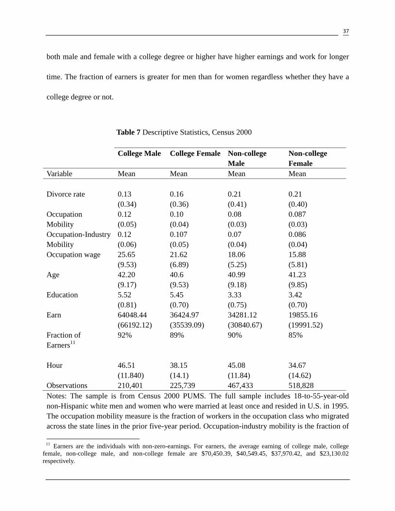
37
both male and female with a college degree or higher have higher earnings and work for longer
time. The fraction of earners is greater for men than for women regardless whether they have a
college degree or not.
Table 7 Descriptive Statistics, Census 2000
Notes: The sample is from Census 2000 PUMS. The full sample includes 18-to-55-year-old
non-Hispanic white men and women who were married at least once and resided in U.S. in 1995.
The occupation mobility measure is the fraction of workers in the occupation class who migrated
across the state lines in the prior five-year period. Occupation-industry mobility is the fraction of
11
Earners are the individuals with non-zero-earnings. For earners, the average earning of college male, college
female, non-college male, and non-college female are $70,450.39, $40,549.45, $37,970.42, and $23,130.02
respectively.
College Male College Female Non-college
Male
Non-college
Female
Variable Mean Mean Mean Mean
Divorce rate 0.13
(0.34)
0.16
(0.36)
0.21
(0.41)
0.21
(0.40)
Occupation
Mobility
0.12
(0.05)
0.10
(0.04)
0.08
(0.03)
0.087
(0.03)
Occupation-Industry
Mobility
0.12
(0.06)
0.107
(0.05)
0.07
(0.04)
0.086
(0.04)
Occupation wage 25.65
(9.53)
21.62
(6.89)
18.06
(5.25)
15.88
(5.81)
Age 42.20
(9.17)
40.6
(9.53)
40.99
(9.18)
41.23
(9.85)
Education 5.52
(0.81)
5.45
(0.70)
3.33
(0.75)
3.42
(0.70)
Earn 64048.44
(66192.12)
36424.97
(35539.09)
34281.12
(30840.67)
19855.16
(19991.52)
Fraction of
Earners11
92% 89% 90% 85%
Hour 46.51
(11.840)
38.15
(14.1)
45.08
(11.84)
34.67
(14.62)
Observations 210,401 225,739 467,433 518,828

38
workers in that occupation-industry class who migrated across state lines in the same period.
Occupation wage is the average wage in each occupation, which is computed among workers
between $3 and $300 per hour. Education level is scaled from 1-8 from less than high school,
some high school, some college, college degree, bachelor’s degree, master’s degree, professional
degree, to doctoral degree.
2.3.2 Methods with Census 2000
The following linear probability model is used as the baseline to estimate the effect of
occupation mobility on an individual’s divorce status.12
𝑑𝑖𝑣𝑜𝑟𝑐𝑒𝑖𝑜𝑠 =∝0+∝1 𝑀𝑜 +∝2 𝑊𝑎𝑔𝑒𝑜 +∝3 𝑒𝑎𝑟𝑛𝑖𝑜𝑠 +∝4 ℎ𝑜𝑢𝑟𝑖𝑜𝑠 + 𝑋𝑖𝑜𝑠𝜃 + 𝑆𝑡𝑎𝑡𝑒𝑠𝛿 +
𝑆𝑡𝑎𝑡𝑒𝑠 ∗ 𝑈𝑟𝑏𝑎𝑛𝑖𝛾 + 휀𝑖𝑜𝑠
(3)
Where for person i in an occupation o, living in state s, 𝑀𝑜 is the occupation mobility and
𝑊𝑎𝑔𝑒𝑜 is the logarithmic occupation wage; 𝑒𝑎𝑟𝑛𝑖𝑜𝑠 is an individual’s logged earnings;
ℎ𝑜𝑢𝑟𝑖𝑜𝑠 is the individual’s weekly working hours. 𝑋𝑖𝑜𝑠 is a vector of demographic controls
including age, age squared, education level as well as the interaction between age and education.
State and state-urban fixed effects are added in order to control for both across state and within
state urban-rural differences in divorce. Two additional controls: children under six or children
between six and 18 are included for women. We estimate Equation 3 separately for college males,
non-college males, college females and non-college females. 13
Personal earnings and weekly working hours are included in Equation 3 because they are
12
Note that in Chapter 2 and Chapter 3, the results are reported by education categories instead of the career
occupation categories in Chapter 1. It is mainly because in NLSY data, the sample size for career couples is too small
to be made comparison with the other groups. 13
All Standard errors are clustered at the occupation level.

39
possibly correlated with one’s occupational characteristics and can affect family divorce
decisions. For example, it is likely that people are in general better compensated for working in
more mobile occupations. Notice that controlling for occupation wage, to some extent, already
alleviates our concerns. In addition, earnings and weekly working hours are post-divorce
information, and there may exist a feedback effect from divorce to one’s post-divorce working
hours and earnings. Therefore we have excluded personal earnings and weekly hours from
Equation 4 (By the same token, child dummies are excluded from female groups).
𝑑𝑖𝑣𝑜𝑟𝑐𝑒𝑖𝑜𝑠 =∝0+∝1 𝑀𝑜 +∝2 𝑊𝑎𝑔𝑒𝑜 + 𝑋𝑖𝑜𝑠𝜃 + 𝑆𝑡𝑎𝑡𝑒𝑠𝛿 + 𝑆𝑡𝑎𝑡𝑒𝑠 ∗ 𝑈𝑟𝑏𝑎𝑛𝑖𝛾 + 휀𝑖𝑜𝑠
(4)
Another concern is the unobserved heterogeneity. People in different occupations may differ in
other ways that affect divorce. For example, it is possible that those working in higher- mobility
occupations do prefer for children, career investment and stability. This might lower the
probability of divorce. In order to control for such unobserved heterogeneity, we put occupation
fixed effect in Equation 5, and use occupation-industry mobility to allow for variation of
mobility within the occupation-industry cell, rather than just across occupations,
𝑑𝑖𝑣𝑜𝑟𝑐𝑒𝑖𝑜𝑛𝑠 =∝0+∝1 𝑀∗𝑖𝑜𝑛𝑠 +∝2 𝑊𝑎𝑔𝑒∗
𝑖𝑜𝑛𝑠+ 𝑋𝑖𝑜𝑛𝑠𝜃 + 𝑂𝑐𝑐𝑖 + 𝑆𝑡𝑎𝑡𝑒𝑠𝛿 + 𝑆𝑡𝑎𝑡𝑒𝑠 ∗
𝑈𝑟𝑏𝑎𝑛𝑖𝛾 + 휀𝑖𝑜𝑛𝑠 (5)
where 𝑀∗𝑖𝑜𝑛𝑠 denotes one’s occupation-industry mobility, and 𝑊𝑎𝑔𝑒∗
𝑖𝑜𝑛𝑠 is now the
corresponding occupation-industry wage.

40
2.3.3 Results with Census 2000
The results for Equation 3 are reported in Table 8. Overall, a husband’s occupation mobility
does not have a significant effect on his divorce status, while wife’s occupation mobility is
positively associated with her divorce status.14
In particular, occupation mobility has a larger
effect on the divorce status of non-college women than on divorce status of college women. For a
non-college-educated woman, increasing the occupation mobility by one standard deviation (.04)
raises her probability of being divorced by 2.24 percentage points.15
In contrast, for a
college-educated woman, the same increase in the occupation mobility increases her probability
of being divorced by 1.24 percentage points. Finally, in each group, the occupation wage is
negatively associated with a person’s divorce status with the impact being statistically
insignificant among college men.16
14 The coefficient of college-educated men’s occupation mobility is significantly different from that of college-educated
women, (F-statistics is 5.37). The coefficient of non-college-educated men’s occupation mobility is significantly different from
that in non-college-educated women, (F-statistics is 18.23).
15 This is pooled standard deviation, which is also used in the following interpretations.
16 Logit estimations are also applied in addition to Linear Probability Models. The results are similar to the conclusion of OLS
estimates. For example, the effect of occupational mobility on college men is insignificantly negative (-.47), and the effect on
non-college men is .87 and significant. Comparing the effect of occupation mobility on college and non-college women, I have
much larger coefficient among non-college-educated women than that of college-educated female peers (5.01 V.S 2.51).

41
Table 8 OLS Estimates of Probability of Divorce Status17
(Controlling for personal earnings and weekly working hours)
Notes: Table 8 provides the coefficients of occupation mobility, occupation wage rate, and
personal earnings from the OLS regression of Equation 3. The sample is as described in Table 7.
The results are reported by gender and by education. Demographic controls includes age, age
squared, education level as well as the interaction between age and education. State and
state-urban fixed effects are also controlled.
Table 9 reports the results of Equation 4, which has the same specification except that it
College male College female Non-college male Non-college female
Mobility -0.08
(0.11)
. 0.31
(0.14)
0.058
(0.08)
0.56
(0.18)
Occ wage -0.01
(0.02)
-0.04
(0.01)
-0.068
(0.009)
0.06
(0.02)
Earn -0.034
(0.002)
0.008
(0.002)
-0.060
(0.002)
0.005
(0.002)
Working Hours
-0.0002
(0.0001)
0.002
(.0003)
. 0.0002
(0.001)
0.003
(.0001)
Children under 18 - -0.125
(0.006)
- -0.128
(0.003)
Children under 6
-
-
-0.09
(0.005)
-
-0.105
(0.002)
Age
0.04
(0.002)
0.04
(0.0004)
0.065
(0.001)
0.05
(0.0001)
Age2
-0.0005
(0.00003)
( -0.0004
(0.00004)
-0.0007
(0.00002)
( -0.0006
(0.00002)
N 194,127 202,675 421,740 445,087

42
excludes personal earnings and weekly work hours as well as children dummies for female
groups. Using Equation 4 occupation mobility significantly increases the probability of divorce
status of non-college men who have been married, while in Equation 3 it has barely an effect on
the divorce status of non-college men when controlling for their personal earnings and weekly
working hours in Equation 3. In contrast, for women who are or have been married, results using
both equations indicate that, being in a more mobile occupation significantly increases their
probability of being divorced, with a disproportional effect on non-college-educated females.
Specifically, in Equation 4, increasing the occupation mobility of a non-college-educated female
by one standard deviation (.04) makes her family more likely to break up by 1.8 percentage
points. This is a moderate effect, considering that the average divorce rate among families with
non-college wives is 21%.
For all four cases in Table 9, occupation mobility has a larger and more positive effect on the
divorce status of non-college-educated persons than on that of the college-educated regardless of
gender. A one-standard-deviation (.04) increase in a non-college-educated woman’s occupation
mobility reduces her family’s stability by 1.8 percentage points, while the same
one-standard-deviation increase in a college-educated female’s occupation mobility is associated
with 1.0 percentage point higher family instability. Similar divorce effects are estimated for male
workers, but the coefficient of college-educated men’s occupation mobility is a wrong sign, and
statistically insignificant.
An explanation of why the divorce status of more educated persons is less likely to be
affected by the occupation mobility is provided as follows. All married people have higher
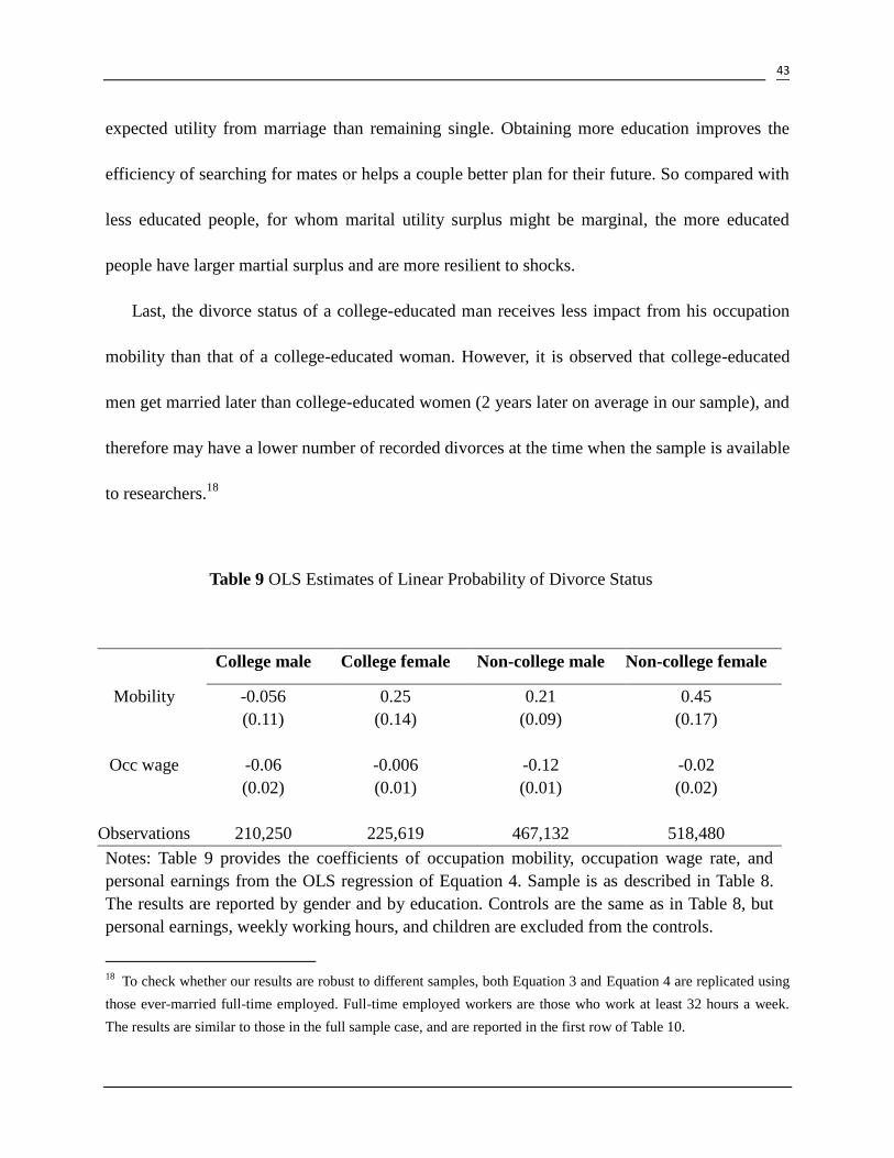
43
expected utility from marriage than remaining single. Obtaining more education improves the
efficiency of searching for mates or helps a couple better plan for their future. So compared with
less educated people, for whom marital utility surplus might be marginal, the more educated
people have larger martial surplus and are more resilient to shocks.
Last, the divorce status of a college-educated man receives less impact from his occupation
mobility than that of a college-educated woman. However, it is observed that college-educated
men get married later than college-educated women (2 years later on average in our sample), and
therefore may have a lower number of recorded divorces at the time when the sample is available
to researchers.18
Table 9 OLS Estimates of Linear Probability of Divorce Status
18
To check whether our results are robust to different samples, both Equation 3 and Equation 4 are replicated using
those ever-married full-time employed. Full-time employed workers are those who work at least 32 hours a week.
The results are similar to those in the full sample case, and are reported in the first row of Table 10.
College male College female Non-college male Non-college female
Mobility -0.056
(0.11)
0.25
(0.14)
0.21
(0.09)
0.45
(0.17)
Occ wage -0.06
(0.02)
-0.006
(0.01)
-0.12
(0.01)
-0.02
(0.02)
Observations 210,250 225,619 467,132 518,480
Notes: Table 9 provides the coefficients of occupation mobility, occupation wage rate, and
personal earnings from the OLS regression of Equation 4. Sample is as described in Table 8.
The results are reported by gender and by education. Controls are the same as in Table 8, but
personal earnings, weekly working hours, and children are excluded from the controls.

44
(Without controlling for personal earnings, weekly working hours, and children)
Table 10 reports the coefficient estimates of occupation-industry mobility based on Equation 5,
using the full-time employed sample. To alleviate the concern on personal endogenous selection
of an occupation or/and an industry, the third row reports results controlling for occupation fixed
effect, and the fourth row does a similar job by including both occupation and industry fixed
effects.
There are several interesting findings. For both genders, mobility effects are larger for workers
without a college degree than college-educated workers. For instance, in Row 2, a
one-standard-deviation (.04) increase in occupation-industry mobility raises the divorce of
non-college-educated women rate by 1.12 percentage points; while, the same increase is only
associated with a rise of .84 percentage point of divorce rate among families with
college-educated women. The effects estimated using models with the fixed-effects are
considerably smaller in magnitude than without fixed-effects. In particular, controlling for both
occupation and industry fixed effects, occupation-industry mobility now reduces the probability
of being married for college-educated female and non-college-educated female by coefficient
estimates of .05 and .064 respectively. Moreover, for a non-college-educated male the effect
becomes larger than that for a non-college-educated female. A one-standard-deviation (.04)
increase in the occupation-industry mobility raises the probability of divorce status by a .4
percentage point.

45
Table 10 The Effects of Mobility on Divorce Status, Fixed Effect Model19
College
male
College
female
Non-college
male
Non-college
female
Occupation mobility -0.06
(0.11)
0.37
(0.18)
0.19
(0.09)
0.52
(0.17)
Occupation-Industry mobility -0.022
(0.046)
0.21
(0.07)
0.089
(0.02)
0.28
(0.06)
Occupation-industry mobility controlling
for occupation fixed effects
0.007
(0.015)
0.1
(0.02)
0.17
(0.03)
0.18
(0.03)
Occupation-industry mobility controlling
for occupation and industry fixed effects
-0.01
(0.02)
0.05
(0.02)
0.10
(0.02)
0.064
(0.02)
Notes: The results of Table 10 are based on the sample in Table 8 and Table 9 but include
full-time employed workers only. The first row reports the coefficients of occupation mobility as
in Equation 4. The second row reports the coefficients of Occupation-Industry mobility as in
Equation 5. Based on specification of Equation 5, the third row reports results controlling for
occupation fixed effect, and the fourth row does a similar job by including both occupation and
industry fixed effects. For each row, personal earnings, weekly working hours and children
controls are excluded.
We also estimate the coefficient of mobility for the old (at least 35) and the young (under 35)
separately. In most cases, the effect of mobility on one’s divorce status is higher for the relatively
old than for the young. This is not surprising, given the fact that spouses of the old are typically
older and may have invested more on location-specific human capital than spouses of the young.
Ceteris paribus, the older spouses are more likely to resist a possible future migration, resulting
in more marriage instability.
19
Standard errors are clustered in the occupation-industry level for Row 2 to Row 4.

46
Chapter Three
3.1 Empirical Analysis Using NLSY79 Data
The analysis in this section uses NLSY79 data covering the period of 1979-2006. NLSY79 is a
nationally representative sample of 12,686 young men and women who were 14-22 years old
when they were first surveyed in 1979. These individuals were interviewed annually through
1994 and have been interviewed on a biennial basis since 1994.
NLSY79 has several advantages over the Census. First, with Census data, it is impossible to
separate re-marriage from first marriage;however, NLSY79 contains each individual’s marriage
history and thus allows us to separately study divorce after first marriage. The examination of
first marriage is important in this dissertation for at least two reasons: 1) before first marriage,
most persons and their spouses have already had an occupation that probably is exogenous to the
formation of first marriage; 2) some people may endogenously choose or adjust their occupations
after the unsuccessful first marriage and hence better prepare for re-marriage. Second, unlike the
Census, NLSY79 reports the information on spouse’s occupation, even for divorced couples.
Third, pre-marriage migration history can be used as a proxy for one’s taste for migration and be
controlled for. Finally, pre-divorce occupation and/or industry information, as well as other
useful individual characteristics are accessible in NLSY79. A major disadvantage of NLSY79,
however, is the smaller sample with less statistical power. One may also be concerned with the
relatively young sample in NLSY79, which cannot represent the whole population in the U.S.
It is assumed in this paper that all else equal, higher occupation mobility is more likely to
result in the conflicts of optimal location choices between two married spouses, and thus tends to

47
generate larger marital instability. Nonetheless, whether occupation mobility should be
interpreted as an exogenous occupational characteristic or as the selection of workers with
similar low migration costs into the same occupation is open to discussion. It is possible that our
measure of occupation mobility is correlated with one’s unobserved preferences for migration,
which in turn affects one’s marital stability. To address this unobserved heterogeneity, the
restricted geocode data from NLSY is used to control for one’s migration history before the first
marriage as a proxy for one’s taste for migration. In a way, this technique is similar to the
analysis by Farber (1994), who uses ―prior job change‖ variables to account for one’s taste for
job changes in the study of the causal effect of job tenure on job separation.
3.1.1 Descriptive Statistics
The sample used in our primary analysis contains individuals who ever report first marriages
and are not in the military sample. Individuals whose spouses were in the military during their
year of first marriage are also excluded from the analysis. Among 8,724 ever-married individuals,
5,561 report valid personal occupation and industry information and their spouses’ occupation
information.20
Since this study focuses on how occupation mobility affects the probability of
divorce, we merge occupation mobility and wage rate as well as the corresponding
industry-occupation characteristics from 5% PUMS of three rounds of Census into the NLSY
data sets. Specifically, for first marriages during 1979 and 1985, occupation mobility,
industry-occupation mobility and wage rate are calculated from the 1980 Census data set; for
20 Spouses’ industry information is not available from NLSY79.

48
first marriages between 1986 and 1995, these occupation and industry-occupation features are
computed using the 1990 Census data set; and the 2000 Census data set is used to provide the
occupation and industry-occupation mobility and wage rate for first marriages after 1995.
Table 11 reports the descriptive statistics. For individuals whose occupation, industry, and
income are not available at the year of first marriage, the most recent information from the prior
five years is used. Since spouses’ past occupational information is not reported, we are unable to
fill spouses’ missing value. Using mobility and wage rate in the industry-occupational cell
substantially decreases the sample size more than that in the occupation cell because some
industry-occupation combination information is not available in the Census 5% PUMS.
Individual controls also include the highest grade completed, highest grade completed by
spouses, age at the first marriage, race indicators, on indicator of living with both biological
parents at age 14, and the expected number of children in 1979.
There is a slightly higher divorce rate among women who are or have been married in our
sample than once or currently married men. An explanation is that women usually marry ealier,
have a longer period of being observed in our sample, and therefore are more likely to have
reported divorced. Occupation mobility and industry-occupation mobility are a little bit higher
among women on average, and this finding is also true for their spouses in terms of occupation
mobility. Men’s average occupation wage rate and industry-occupation wage rate are higher than
that of women. For average individual annual income, men enjoy a nearly three quarters
premium compared with women. One possible reason is that men who have been or are married
work more hours than married women in our sample. The average individual income of women

49
is about 58% lower than that of their spouses in the women’s sample; whereas, men earn 75%
more than their spouses in the first year of their marriage in the men’s sample.
Table 11 Descriptive Statistics for Variables in Cross-section Regressions
Women Men
Mean Standard
Deviation
Mean Standard
Deviation
Percent divorced from first
marriage
0.36 0.35
Age of first marriage 23.8 (4.87) 24.9 (4.82)
Year of first marriage 1985 (4.96) 1986 (5.08)
Duration of first marriage in
years (if divorced)
7.89 (5.67) 7.69 (5.31)
Occupation mobility 0.22 (0.09) 0.20 (0.09)
Occupation wage rate 9.06 (4.1) 10.89 (4.4)
Spouses’ occupation
mobility
0.22 (0.09) .20 (0.09)
Spouses’ occupation wage
rate
10.79 (4.63) 9.49 (4.54)
Income 12,267 (11,165) 21052 (11,450)
Working hour (weekly) 32 (12) 39 (12)
Percent of black 0.19 0.20
Percent of Hispanic 0.15 0.14
Highest grade completed 13.31 (2.14) 13.02 (2.44)
Spouses’ highest grade
completed
13 (4.2) 13 (3.2)
Percent living with both
biological parent in 1979
0.72 0.72
Number of Children
expected (measured 1979)
2.4 (1.44) 2.36 (1.43)
Industry-occupation
mobility
0.24 (0.14) 0.22 (0.16)
Industry-occupation wage
rate
8.86 (4.42) 10.76 (4.9)
Spouses’ income 19,207 (17,244) 12,158 (13,173)
Spouses’ working hour
(weekly)
40 (14.00) 34 (12)
N 2,194 2,072
Notes: The sample includes individuals who ever report first marriages in NLSY79 and are not in
50
military sample. Individuals whose spouses were in the military during their year of first
marriage are excluded from the analysis. Occupation/industry-occupation mobility and wage
rates are from 5% PUMS of three rounds of census: Census 1980 is used for those with first
marriages before 1986; for the first marriages between 1986 and 1995, 1990 Census is used; and
the 2000 Census data set is used to provide the occupation and industry-occupation mobility and
wage rate for first marriages after 1995.
3.1.2 Information in the Geocode Files of NLSY79
The Geocode files of NLSY79 provide us with migration information that the public-use files
do not. To be specific, the history before his/her first marriage can be constructed using the
Geocode data.21
We argue that to some extent this migration history can reflect and thus be
treated as a proxy for one’s preference for migration. Recall that in using Census data, individual
heterogeneity in preferences for migration is one of the main confounding factors in the OLS
regression of marriage status on one’s own spousal occupation mobility. This is because the
selection of one’s occupation in part due to migration preferences, and such prefer can also affect
family stability. Being able to control heterogeneity in the taste for migration should have the
potential to lessen concern on identifying the real causal effect of occupation mobility on one’s
marriage.
We create two different sets of controls for prior migration history. One consists of indicators
of the number of pre-marriage migrations; the other is the duration (in years) since the most
recent pre-marriage migration. Notice that this approach is analogous but not equivalent to what
Farber (1994) does in the identification of the causal effect of job tenure on the probability of job
separation. In that paper, he actually controls for the number of prior jobs started in each year
21
Migration preferences are assumed to be constant over time.
51
preceding the start of the current job.
3.1.3 Methodologies Overview
Following McKinnish (2007), the regression analysis includes two parts: a linear probability
model using cross-sectional data and a discrete-time hazard model using panel data. In the linear
probability model, the information of respondents’ occupation, industry and location at the time
of first marriage is used. Unlike work and location decisions made during the marriage, these
decisions before or at the time of first marriage may be less endogenous to the quality or stability
of the marriage. But, if one believes that occupation and location at the year of divorce are more
likely to affect people’s divorce decision, then the linear probability model becomes problematic.
To address this possibility, we also use a discrete-time hazard model to predict how likely a
person will end up divorced in a certain year when she/he remained married in the past year,
controlling for occupation and personal characteristics in that current year.
Economic control variables such as individual and spouses income and working hours are also
available in NLSY79. As discussed when using Census data, since these economic controls could
be correlated with both marriage status and occupation/industry characteristics, adding them into
the linear probability models will help reduce the omitted variable bias. However, one’s income
reported in NLSY79 is the occupation income or income from the major occupation (if he/she
has at least two occupations). If there are only small income or working-hour variations within
an occupation, controlling occupation fixed-effects already purges mean income and mean
working hours in that occupation. In addition, the reverse causality of an unsuccessful marriage
on one’s income and working hours cannot be simply ignored. An example is that one can adjust

52
working hours and thus income, forecasting a divorce in the near future. In the following
regression, we will separately test the effect of occupation mobility with and without personal
economic controls.
Although actual migration may affect one’s marriage stability, it should not enter the
right-hand side of the divorce regression. The reason is that actual migration is more likely to be
correlated with unobserved personal characteristics and family structure that lead to divorce; plus
there is reverse causality from an unstable marriage to actual migration. Since the Geocode files
provide information on the specific date of respondents’ (first) marriage(s), we can separate
respondents who actually migrate after their first marriage from those who do not do so. Thus,
potentially different patterns of marital stability between migrants and non-migrants can be
investigated in detail.
3.1.4 Regression Specifications
Baseline Regressions
The baseline regression considers a linear probability model. Equation 6 estimates the effect of
occupation mobility on divorce status controlling for occupation wage rate and individual
characteristics as well as state,1-digit occupation, and 1-digit industry fixed effects.
𝑌𝑖𝑜𝑛𝑠 =
𝛽0 + 𝛽1𝑜𝑐𝑐_𝑚𝑜𝑏𝑖𝑙𝑖𝑡𝑦𝑜 + 𝛽2𝑜𝑐𝑐_𝑤𝑎𝑔𝑒𝑜 + 𝛽3𝑜𝑐𝑐_𝑚𝑜𝑏𝑖𝑙𝑖𝑡𝑦_𝑠𝑝𝑜𝑢𝑠𝑒𝑜 +
𝛽4𝑜𝑐𝑐_𝑤𝑎𝑔𝑒_𝑠𝑝𝑜𝑢𝑠𝑒𝑜 + 𝑖𝑛𝑐𝑜𝑚𝑒𝑖𝛽5 + 𝑖𝑛𝑐𝑜𝑚𝑒_𝑠𝑝𝑜𝑢𝑠𝑒𝑖𝛽6 + ℎ𝑜𝑢𝑟𝑖𝛽7 + ℎ𝑜𝑢𝑟_𝑠𝑝𝑜𝑢𝑠𝑒𝑖𝛽8 +
𝑐𝑜𝑛𝑡𝑟𝑜𝑙𝑖𝛽9 + STATEsδ + (STATEs ∗ 𝑈𝑟𝑏𝑎𝑛𝑖)∅ + occoγ1 + indnγ2 + occ_spouseoγ3 + εi

53
(6)
Where for person i in occupation o and industry n, living in state s, 𝑌𝑖𝑜𝑛𝑠 is an indicator that
equals one if the individual reports ending their first marriage in divorce at any time in the
NLSY79 survey. 𝑀𝑜𝑏𝑖𝑙𝑖𝑡𝑦𝑜 is occupation mobility of the respondent’s occupation at the year of
first marriage. 𝑊𝑎𝑔𝑒_𝑠𝑝𝑜𝑢𝑠𝑒𝑜 denotes occupation wage rate of the respondent’s occupation at
the year of his/her first marriage. 𝑀𝑜𝑏𝑖𝑙𝑖𝑡𝑦_𝑠𝑝𝑜𝑢𝑠𝑒𝑜 and 𝑤𝑎𝑔𝑒_𝑠𝑝𝑜𝑢𝑠𝑒𝑜 are occupation
variables with respect to spouses’ occupation at the year of their first marriage. 𝐼𝑛𝑐𝑜𝑚𝑒𝑖 and
𝑖𝑛𝑐𝑜𝑚𝑒_𝑠𝑝𝑜𝑢𝑠𝑒𝑖 are the annual income from wages and salary in logarithm for respondents and
their spouses. 𝐻𝑜𝑢𝑟𝑖 and ℎ𝑜𝑢𝑟_𝑠𝑝𝑜𝑢𝑠𝑒𝑖 are the number of hours worked during the year of
marriage in logarithm for respondents and their spouses. 𝐶𝑜𝑛𝑡𝑟𝑜𝑙𝑖 are individual controls
including highest grade completed, highest grade completed by spouse, age at first marriage, race
indicators, an indicator of living with both biological parents at age 14, whether living in the
South at age 14, and the expected number of children in 1979.
STATEs is a vector of state indicator variables, and STATEs ∗ 𝑈𝑟𝑏𝑎𝑛𝑖 is the interaction
between state and urban fixed-effects. Since 𝑜𝑐𝑐_𝑚𝑜𝑏𝑖𝑙𝑖𝑡𝑦𝑜, 𝑜𝑐𝑐_𝑤𝑎𝑔𝑒𝑜 , 𝑚𝑜𝑏𝑖𝑙𝑖𝑡𝑦_𝑠𝑝𝑜𝑢𝑠𝑒𝑜
and 𝑤𝑎𝑔𝑒_𝑠𝑝𝑜𝑢𝑠𝑒𝑜 are measured using three-digit level occupations, occo and indn are
measured in one-digit level in order to avoid perfect multi-collinearity. As a consequence, the
value of mobility and wage rate can vary within broader occupation and industry cells.
To address the potential reverse causality arising from adding economic controls, we also
estimate Equation 7 in which individuals’ and spouses’ income and working hours are excluded.

54
𝑌𝑖𝑜𝑛𝑠 = 𝛽0 + 𝛽1𝑜𝑐𝑐_𝑚𝑜𝑏𝑖𝑙𝑖𝑡𝑦𝑜 + 𝛽2𝑜𝑐𝑐_𝑤𝑎𝑔𝑒𝑜 + 𝛽3𝑜𝑐𝑐_𝑚𝑜𝑏𝑖𝑙𝑖𝑡𝑦_𝑠𝑝𝑜𝑢𝑠𝑒𝑜
+ 𝛽4𝑜𝑐𝑐_𝑤𝑎𝑔𝑒_𝑠𝑝𝑜𝑢𝑠𝑒𝑜 + 𝑐𝑜𝑛𝑡𝑟𝑜𝑙𝑖𝛽5 + STATEsδ + (STATEs ∗ 𝑈𝑟𝑏𝑎𝑛𝑖)∅
+ occoγ1 + indnγ2 + occ_spouseoγ3 + εi
(7)
Similar to the analysis of using Census data, Equation 8 differs from Equation 7 by instead
using the industry-occupation mobility and the industry-occupation wage rate to account for the
mobility differences at the occupation level within the same industry, and vice versa.
𝑌𝑖𝑜𝑛𝑠 = 𝛽0 + 𝛽1𝑖𝑛𝑑_𝑜𝑐𝑐_𝑚𝑜𝑏𝑖𝑙𝑖𝑡𝑦𝑜𝑛 + 𝛽2𝑖𝑛𝑑_𝑜𝑐𝑐_𝑤𝑎𝑔𝑒𝑜𝑛 + 𝛽3𝑜𝑐𝑐_𝑚𝑜𝑏𝑖𝑙𝑖𝑡𝑦_𝑠𝑝𝑜𝑢𝑠𝑒𝑜
+ 𝛽4𝑜𝑐𝑐_𝑤𝑎𝑔𝑒_𝑠𝑝𝑜𝑢𝑠𝑒𝑜 + 𝑐𝑜𝑛𝑡𝑟𝑜𝑙𝑖𝛽4 + STATEsδ + (STATEs ∗ 𝑈𝑟𝑏𝑎𝑛𝑖)∅
+ occoγ1 + indnγ2 + occ_spouseoγ3 + εi
(8)
Pre-Marriage Migration History
If the pre-marriage migration history is a proxy for one’s preference for migration, people with
more such migrations or with more recent one are more likely to have post-marriage migration.
Alternatively, the learning-by-doing migration could offer the other side of story: those who
migrate more frequently before their first marriage are more likely to choose their post-marriage
destination successfully, and thus more likely to enjoy a stable marriage.
Equation 9 is used to test those two competing hypotheses. Dependent variable 𝑃𝑜𝑠𝑡_𝑚𝑖𝑔𝑖𝑜𝑛𝑠
is an indicator which has a value of one if a respondent reports a cross-state migration five years
after his/her first marriage. There are two main sets of explanatory variables: occupation mobility
and pre-marriage migration history. Occupation mobility consists of one’s own occupation

55
mobility (𝑜𝑐𝑐_𝑚𝑜𝑏𝑖𝑙𝑖𝑡𝑦𝑜) and spousal occupation mobility (𝑜𝑐𝑐_𝑚𝑜𝑏𝑖𝑙𝑖𝑡𝑦𝑠𝑝𝑜𝑢𝑠𝑒𝑜) at the time of
the first marriage. Pre-marriage migration history (𝑝𝑟𝑒_𝑚𝑖𝑔) includes three migration dummies:
whether the respondent migrated once, twice, or more three years before first marriage. This
arrangement allows each additional migration to have a different effect on post-marriage
migration. Other controls include occupation wage rate for both parties, state fixed effects, urban
fixed effects, occupation fixed effects for both parties, highest education completed by both
parties, the age and the year of first marriage, race indicators and a dummy indicating living in
the South at age 14.
𝑃𝑜𝑠𝑡_𝑚𝑖𝑔𝑖𝑜𝑛𝑠 =
𝛽0 + 𝛽1𝑜𝑐𝑐_𝑚𝑜𝑏𝑖𝑙𝑖𝑡𝑦𝑜 + 𝛽2𝑜𝑐𝑐_𝑚𝑜𝑏𝑖𝑙𝑖𝑡𝑦𝑠𝑝𝑜𝑢𝑠𝑒𝑜+
𝑝𝑟𝑒_𝑚𝑖𝑔𝛽3 + 𝛽4𝑜𝑐𝑐𝑤𝑎𝑔𝑒𝑜+ 𝛽5𝑜𝑐𝑐𝑤𝑎𝑔𝑒𝑠𝑝𝑜𝑢𝑠𝑒𝑜
+ 𝑖𝑛𝑑𝑖𝑣𝑖𝑑𝑢𝑎𝑙 𝑐𝑜𝑛𝑡𝑟𝑜𝑙𝑖𝛽6 + 𝑠𝑡𝑎𝑡𝑒𝑠𝛿 +
(𝑠𝑡𝑎𝑡𝑒𝑠 ∗ 𝑢𝑟𝑏𝑎𝑛𝑖)∅ + 𝑜𝑐𝑐𝑜𝛾1 + 𝑜𝑐𝑐𝑠𝑝𝑜𝑢𝑠𝑒𝑜𝛾2 + 휀𝑖
(9)
Results are shown in Table 12 for the sample of all respondents who report their first
marriages between 1983 and 1996 in NLSY79. This period is chosen so that each respondent can
have consecutive three years to be observed on migration(s). Having migrated once, twice, or
three times are the three dummies of pre-marriage migration. The first two columns report the
effects of pre-marriage migration history for males and for females separately. The last two
columns are the effects for a smaller group of respondents whose first marriages did not break up
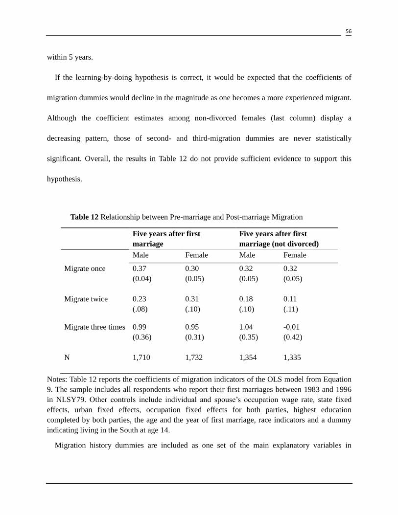
56
within 5 years.
If the learning-by-doing hypothesis is correct, it would be expected that the coefficients of
migration dummies would decline in the magnitude as one becomes a more experienced migrant.
Although the coefficient estimates among non-divorced females (last column) display a
decreasing pattern, those of second- and third-migration dummies are never statistically
significant. Overall, the results in Table 12 do not provide sufficient evidence to support this
hypothesis.
Table 12 Relationship between Pre-marriage and Post-marriage Migration
Notes: Table 12 reports the coefficients of migration indicators of the OLS model from Equation
9. The sample includes all respondents who report their first marriages between 1983 and 1996
in NLSY79. Other controls include individual and spouse’s occupation wage rate, state fixed
effects, urban fixed effects, occupation fixed effects for both parties, highest education
completed by both parties, the age and the year of first marriage, race indicators and a dummy
indicating living in the South at age 14.
Migration history dummies are included as one set of the main explanatory variables in
Five years after first
marriage
Five years after first
marriage (not divorced)
Male Female Male Female
Migrate once 0.37
(0.04)
0.30
(0.05)
0.32
(0.05)
0.32
(0.05)
Migrate twice 0.23
(.08)
0.31
(.10)
0.18
(.10)
0.11
(.11)
Migrate three times 0.99
(0.36)
0.95
(0.31)
1.04
(0.35)
-0.01
(0.42)
N 1,710 1,732 1,354 1,335
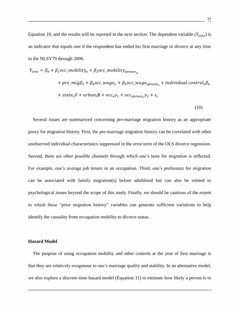
57
Equation 10, and the results will be reported in the next section. The dependent variable (𝑌𝑖𝑜𝑛𝑠) is
an indicator that equals one if the respondent has ended his first marriage in divorce at any time
in the NLSY79 through 2006.
𝑌𝑖𝑜𝑛𝑠 = 𝛽0 + 𝛽1𝑜𝑐𝑐_𝑚𝑜𝑏𝑖𝑙𝑖𝑡𝑦𝑜 + 𝛽2𝑜𝑐𝑐_𝑚𝑜𝑏𝑖𝑙𝑖𝑡𝑦𝑠𝑝𝑜𝑢𝑠𝑒𝑜
+ 𝑝𝑟𝑒_𝑚𝑖𝑔𝛽3 + 𝛽4𝑜𝑐𝑐_𝑤𝑎𝑔𝑒𝑜 + 𝛽5𝑜𝑐𝑐_𝑤𝑎𝑔𝑒𝑠𝑝𝑜𝑢𝑠𝑒𝑜+ 𝑖𝑛𝑑𝑖𝑣𝑖𝑑𝑢𝑎𝑙 𝑐𝑜𝑛𝑡𝑟𝑜𝑙𝑖𝛽6
+ 𝑠𝑡𝑎𝑡𝑒𝑠𝛿 + 𝑢𝑟𝑏𝑎𝑛𝑖∅ + 𝑜𝑐𝑐𝑜𝛾1 + 𝑜𝑐𝑐𝑠𝑝𝑜𝑢𝑠𝑒𝑜𝛾2 + 휀𝑖
(10)
Several issues are summarized concerning pre-marriage migration history as an appropriate
proxy for migration history. First, the pre-marriage migration history can be correlated with other
unobserved individual characteristics suppressed in the error term of the OLS divorce regression.
Second, there are other possible channels through which one’s taste for migration is reflected.
For example, one’s average job tenure in an occupation. Third, one’s preference for migration
can be associated with family migration(s) before adulthood but can also be related to
psychological issues beyond the scope of this study. Finally, we should be cautious of the extent
to which these ―prior migration history‖ variables can generate sufficient variations to help
identify the causality from occupation mobility to divorce status.
Hazard Model
The purpose of using occupation mobility and other controls at the year of first marriage is
that they are relatively exogenous to one’s marriage quality and stability. In an alternative model,
we also explore a discrete-time hazard model (Equation 11) to estimate how likely a person is to

58
divorce in a certain year given that his/her first marriage remained intact in the past year,
controlling for occupation, industry and personal characteristics in the current year.
H(t) = Pr(Divorce in year t|Married but Not Divorced in Year t − 1)
= F[𝛽0 + 𝛽1𝑚𝑜𝑏𝑖𝑙𝑖𝑡𝑦𝑜𝑡 + 𝛽2𝑤𝑎𝑔𝑒𝑜𝑡 + 𝛽1𝑚𝑜𝑏𝑖𝑙𝑖𝑡𝑦𝑠𝑝𝑜𝑢𝑠𝑒𝑜𝑡+ 𝛽2𝑤𝑎𝑔𝑒𝑠𝑝𝑜𝑢𝑠𝑒𝑜𝑡
+ 𝑐𝑜𝑛𝑡𝑟𝑜𝑙𝑖𝛽3 + STATEstδ + (STATEst ∗ 𝑈𝑟𝑏𝑎𝑛𝑖𝑡)∅ + occotγ1 + indntγ2
+ occspouseotγ3 + Yeartλ + g(Yeart − year of marriagei) + εi
(11)
for person i working in occupation o and industry n, living in state s in year t.
Equation 11 contains an individual’s occupation mobility and wage rate for both an individual
and the spouse. State and urban controls as well as occupational and industry fixed effects are all
measured at time t. Individual controls are the same as those when using Census 2000 in
Equations 3 and Equation 4. Year effects are also included in the model. We consider a
non-parametric baseline and create g(.) as a vector of dummy variables for the duration of
marriage, where the hazard is assumed to be constant after ten years of marriages. Discrete-time
logit estimation is applied in which the right censor is assumed, and the "hazard" is getting
divorced in a certain year.
The hazard model applies unbalanced panel data. People who got married before 1979 could
be included in this panel data as long as they didn't divorce prior to 1979. Occupational and
industry information for the current year is used. If this information is not available from the
individual or his/her spouse for a specific year, the most recent occupation or industry reported in

59
the past five (5) years will be used. This approach avoids selection bias in labor force
participation. The disadvantage is that we might estimate how the past occupations instead of the
present ones affect the marital stability of those respondents. Observations are dropped if there is
no individual occupation or spousal occupation available for the past five years.
3.2 Results of NLSY79
Baseline Regression Results
Some preliminary results of Equations 7 and 8 are reported in Table 13-1 and Table 13-2
respectively, for the main coefficients of interest in this study. Standard errors are clustered at the
occupational level for Equation 7 and at industry-occupational level for Equation 8. As
mentioned before, we do not control for respondents’ working hours and income in the OLS
regression because this has by and large been done by adding occupation/industry fixed-effects,
and there are possible feedback effects from a (potential) divorce to post-divorce working hours
and earnings. To make a comparison, we first run the regressions without controlling for spouses’
occupation mobility and then include spouses’ occupation mobility. Dummy variables for
pre-marriage migration history, state indicators and state-urban interactions are not included in
these baseline regressions. 22
22 Using Logit to estimate the effect of occupational mobility on divorce, we obtain similar results in which the coefficient for
women is significantly positive, but the coefficient for men is insignificant.

60
Table 13-1 OLS Estimation of Probability of Divorce
(Occupation Mobility)
Table 13-2 OLS Estimation of Probability of Divorce
(Industry-Occupation Mobility)
OLS Estimates of Probability of Divorce, NLSY—without controlling for spouses’
occupation mobility
Male Female
Occupation Mobility 0.10
(0.14)
0.26
(0.14)
OLS Estimates of Probability of Divorce, NLSY—controlling for spouses’ occupation
mobility
Male Female
Occupation Mobility -0.22
(0.25)
0.13
(0.24)
Spouses’ Occupation
mobility
0.39
(0.26)
0.15
(0.23)
N=2611 N=2765
OLS Estimates of Probability of Divorce, NLSY—without controlling for spouses’
occupation mobility
Male Female
Industry-Occupation
mobility
0.03
(0.06)
0.14
(0.07)
OLS Estimates of Probability of Divorce, NLSY—controlling for spouses’ occupation
mobility
Male Female
Industry-Occupation
mobility
-0.05
(0.07)
0.08
(0.08)
Spouses’ occupation
mobility
0.35
(0.15)
0.25
(0.15)
N=2487 N=2673

61
Notes: Sample is the same as in Table 11. Coefficients of the individual and spouse’s occupation
mobility/industry-occupation mobility are reported from Equation 7 and Equation 8. Individuals’
occupation/industry-occupation wage rate and spouses’ occupation wage rates are controlled.
Individual controls including highest grade completed, highest grade completed by spouse, age at
first marriage, race indicators, an indicator of living with both biological parents at age 14,
whether living in the South at age 14, and the expected number of children in 1979.1-digit
occupation, and 1-digit industry fixed effects are included. Standard errors are clustered the
occupational level for Equation 7 and at industry-occupational level for Equation 8.
Both the coefficient estimates for male occupation mobility and for male industry-occupation
mobility are never statistically significant. And in the latter scenario, they even display opposite
signs. Without controlling for the husband’s occupation mobility, the effect of female occupation
mobility is almost statistically significant at 5% level in Equation 7, and the effect of female
industry-occupation mobility is almost statistically significant at 1% level in Equation 8.
However, after controlling for the husband’s occupation mobility, neither of the coefficient
estimates is statistically significant at the conventional confidence intervals. A possible
explanation is that since one’s own occupation mobility is highly correlated with the spousal
occupation mobility, controlling for both creates multi-collinearity and results in a large standard
error for the coefficient estimates.23
Regression Results with Geocode Information
Table 14 reports results of Equation 10 with Geocode information using four different samples.
The full sample includes all respondents who reported their first marriage in NLSY79. Columns
23 One may be concerned with whether an individual is in an occupation with higher mobility affects the
significance of the results. To test this, a high mobility indicator—whether the individual or spouse is in occupations
with mobility higher than the mean of all occupations (0.21)— is controlled. Results show that neither the coefficient
of own occupation mobility nor that of spouse’s occupation mobility is statistically significant.

62
3 and 4 report coefficient estimates for these respondents whose first marriage was in or before
1996, because NLSY79 records consecutive migration history every year before 1994 and every
other year after 1994. Since the year of first marriage affects the observed length of migration
history before marriage, we further restrict the sample so that all respondents have equivalent
observed years of pre-marriage migration records. As a result, Columns 5 and 6 are for
respondents who were married for the first time between 1983 and 1996, and whose
pre-marriage migrations can be observed for three consecutive years. As a sensitivity test, the last
two columns report results for respondents whose first marriage occurred between 1985 and
1996, and whose pre-marriage migration(s) can be observed for five consecutive years. In all
four samples, respondents are eliminated if they entered first marriage before starting a formal
work. For those with missing industry or occupational information in the year of their first
marriage, information from their most recent reported job in the past five years is used.
Table14 OLS Estimation of Probability of Divorce Controlling for Pre-marriage Migration
Full Sample First-marriage
before 1996
First-marriage
1983 to 1996
First-marriage
1985 to 1996
Male
(1)
Female
(2)
Male
(3)
Female
(4)
Male
(5)
Female
(6)
Male
(7)
Female
(8)
Own
occupation
mobility
-0.22
(0.25)
0.13
(0.24)
-0.23
(0.27)
0.24
(0.25)
-0.43
(0.29)
0.05
(0.27)
-0.41
(0.31)
0.006
(0.29)

63
Notes: Table 14 reports the result of OLS model from Equation 10 for occupation mobility and
migration indicators. The full sample includes all respondents who reported their first marriage
in NLSY79 with different specifications in marriage periods for the other columns. In addition to
the individual controls in Table 13, state indicators and state-urban interactions are included.
We do not find sufficient evidence that higher pre-marriage occupation mobility (for either
spouse) results in higher instability of first marriage. For male respondents, a higher mobility in
their occupation reduces the instability of the marriage; whereas a higher mobility in the wife’s
occupation makes the marriage more unstable. But both effects are insignificant at the
conventional confidence interval. For female respondents, both own effect and spouse effect are
positive statistically insignificant.
However, this does not necessarily mean the failure of the prediction by Mincer (1978) that
prospective migration may lead to family dissolution. Our measure of occupation mobility,
calculated from several rounds of Census data, is far from being perfect. Also, whether
occupation mobility is a good proxy for prospective migration is an open question. Still, one may
contend whether and to what extent pre-marriage occupation mobility is an appropriate predictor
Spousal
occupation
mobility
0.39
(0.26)
0.15
(0.23)
0.32
(0.28)
0.13
(0.25)
0.43
(0.30)
0.22
(0.27)
0.31
(0.32)
0.22
(0.29)
Migration
once
- - 0.05
(0.04)
-0.01
(0.04)
0.003
(0.03)
0.04
(0.03)
0.05
(0.03)
0.01
(0.04)
Migrate
twice
- - 0.04
(0.05)
0.06
(0.06)
0.17
(0.06)
0.06
(0.08)
0.03
(0.05)
0.04
(0.06)
Migrate
more
- - 0.12
(0.10)
0.08
(0.06)
-0.25
(0.28)
0.005
(0.23)
0.17
(0.11)
0.14
(0.16)
N 2,611 2,765 2,313 2,615 1,710 1,732 1,318 1,211

64
of family divorce, which in general takes place at least several years after first marriage. Finally,
a linear probability model effectively assumes that the marginal effect of occupation mobility is
the same, regardless of the level of occupation mobility.
Can the framework of rational expectation hold? It is possible that for important lifetime
decisions like forming a marital relationship, both spouses have fully expected a potential future
migration due to occupational requirements, and have thus internalized its cost into their
respective optimal location choices. Or they take a unitary approach in the migration decision
and act as if there is only one decision maker. If that is the case for most couples, it won’t be
surprising to see that prospective migration has no effect on marital stability.
To check the robustness of this finding, Table 15 reports results using the most recent
pre-marriage migration as the other measure of pre-marriage migration history. The sample
includes those who were married for the first time between 1983 and 1996. Again, coefficient
estimates of occupation mobility are not statistically significant.

65
Table 15 OLS Estimation of Probability of Divorce Controlling for
Most Recent Pre-marriage Migration
Male Female
Own occupation mobility -0.43
(0.30)
0.04
(0.27)
Spousal occupation mobility 0.43
(0.3)
0.24
(0.27)
Last migration is one year ago 0.05
(0.05)
0.10
(0.05)
Last migration is two-year ago 0.08
(0.06)
0.008
(0.05)
Last migration is three-year ago -0.01
(0.05)
0.02
(0.06)
N 1,710 1,732
Notes: The sample of Table 15 is same as the full sample used in Table 14. Migration frequency
indicators are replaced by most recent pre-marriage migration duration indicators.
Regression Results of Hazard Model
The results using logit discrete hazard model are reported in Table 16. For both male and
female groups, the hazard of getting divorced increases with occupation mobility, but the
coefficients are not statistically significant. The coefficients of male occupation wage rate are
negative, while the coefficients of female occupation wage rates are positive, but both are a
statistically insignificant. The coefficient estimates of spousal occupation mobility and wage rate
are also reported in a similar pattern.

66
Table 16 Discrete Divorce Hazard Model
Male Female
Occupation mobility 1.33
(.78)
1.9
(.68)
Occupation wage rate -0.012
(0.009)
0.0008
(0.007)
Spouse occupation mobility 0.9
(0.76)
0.27
(0.6)
Spouse occupation wage rate 0.004
(0.008)
-0.014
(0.008)
N 27,453 35,102
Notes: The Sample uses ever-married respondents in the NLSY79. Table 16 reports estimates
from a logistic model for divorce from Equation 11. All regressions include the individual’s
occupation and spouse’s occupation mobility, and wage controls, age of marriage, race indicators
(black, Hispanic), highest grade completed, highest grade completed of spouse, indicator for
respondent lived with both biological parents at age 14, expected age of marriage in 1979,
expected number of children in 1979, state fixed-effects, state-urban fixed-effects, year
fixed-effects, duration of marriage indicators, 1-digit industry code fixed-effects, 1-digit
occupation code fixed-effects and 1-digit spouse occupation code fixed-effects.
3.3 Conclusion
This paper uses data from Census 1980 to 2000 and NLSY79 to test the predication by Mincer
(1978) that prospective migration may cause marital instability. For the single round of Census
2000, there is some evidence that the probability of divorce among couples is positively
associated with occupation mobility, and the effect of women’s occupation mobility is larger than
that of men’s. However, the empirical results from using NLSY79 are insignificant under various
econometric specifications with rich controls. Several factors that can prevent the potential
migration effect from being identified are briefly discussed below.

67
First, an occupation already compensates for its higher mobility in terms of some unobserved
benefits like a more flexible work schedule. Second, across occupations people differ in other
ways that also affect divorce but cannot be controlled for given the available data. For example,
occupation mobility is correlated to one’s ability to maintain a marriage. Third, within the same
occupation people differ in their reasons for cross-state migrations; for example, some migrate
because of promotions while others do so simply as a job requirement. That is, occupation
mobility is not a homogeneous measure.
We offer two explanations for the absence of the prospective migration effect. First, it is
possible that before a marriage one is rational and fully expects the costs and benefits from own
future migration and from future migration of the potential spouse; two parties then form a
marital relationship if they are able to internalize the costs of future migration. Second, upon
important family decisions such as migration and giving birth, the husband and the wife take a
unitary approach and act as if there is only one decision maker.

68
References
Aberg, Yvonne. (2003). Social Interactions: Studies of Contextual Effects and Endogenous
Processes (Unpublished doctoral dissertation). Stockholm University, Sweden.
Acemoglu, Daron. (1996). ―A Microfoundation for Social Increasing Returns in Human Capital
Accumulation‖, Quarterly Journal of Economics, CXI, 779-804.
Astrom, Johanna and Olle Westerlund. (2006). ―Sex and Migration: Who is the Tied Mover?‖
Working Paper, Department of Economics, Umea University.
Basker, Emek. 2003. ―Education, Job Search and Migration.‖ University of Missouri-Columbia,
Working Paper 02-16.
Becker, Gary S. (1974). A theory of social interactions. The Journal of Political Economy, 82(6),
1063-1093.
Becker, Gary S., Elisabeth M. Landes and Robert T. Michael. (1977). An economic analysis of
marital instability. The Journal of Political Economy 85(6), 1141-1187.
Bramley, Glen, Tony Champion and Tania Fisher. (2006). Exploring the household impacts of
migration in Britain using panel survey data. Regional Studies 40(8), 907-926.
Compton, Janice and Robert Pollak. ―Why are Power Couples Increasingly Concentrated in
Large Metropolitan Areas?‖ Journal of Labor Economics, Forthcoming.
Cooke, Thomas J. 2003. ―Family Migration and the Relative Earnings of Husbands and Wives.‖
Annals of the Association of American Geographers 93:338-49.
Cooke, Thomas and Karen Speirs. 2005. ―Migration and Employment among the Civilian
Spouses of Military Personnel.‖ Social Science Quarterly 86(2):343-355.
Costa, Dora and Matthew Kahn. (2000). ―Power Couples: Changes in the Location Choice of the
College Educated, 1940-1990.‖ Quarterly Journal of Economics 53(4) 648-664.
Duncan, R. Paul and Carolyn Cummings Perrucci. (1976). Dual occupation families and
migration. American Sociological Review 41(2), 252-261.
Farber, Henry S. (1994). The analysis of interfirm worker mobility. Journal of Labor Economics
12 (4), 554-593.

69
Friedlberg Leora. (1998). Did unilateral divorce raise divorce rates? Evidence from panel data.
The American Economic Review 88(3), 608-627.
Glaeser, Edward L., and David C. Mare. (2001). ―Cities and Skills‖, Journal of Labor
Economics, 19(2): 316-342
Greenwood, Michael J.. (1975). ―Research on Internal Migration in the United States: A Survey.‖
Journal of Economic Literature 13(2): 397-433
Greenwood, Michael J.. (1993). ―Migration: A Review.‖ Regional Studies, 27(4): 295-296
Hill, Laura E. (2004). Connections between U.S. female migration and family formation and
dissolution. Migraciones Internacionales, 2(3), 60-82.
McKinnish, Terra G. (2007). Sexually-integrated workplaces and divorce: Another form of
on-the-job search. Journal of Human Resources XLII(2), 331-352.
McKinnish, Terra G. (2008). Spousal mobility and earnings. Demography 45(4), 829-849.
Michael, Robert T. (1988). Allocation of Income Within the Household.
Mincer, Jacob. (1979). Family migration decisions. The Journal of Political Economy 86(5),
749-773.
Ross Heather L. and Isabel V. Sawhill. (1975). Time of Transition: The Growth of Families
Headed by Women.
Ruggles, Steven. (1997). The rise of divorce and separation in the United States 1880-1990.
Demography 34(4), 455-466.
Sandell, Steven. (1977). ―Women and the Economics of Family Migration.‖ The Review of
Economics and Statistics 59(4): 406-14.
Schwartz, Christine and Robert Mare. (2005). ―Trends in Educational Assortative Marriage.‖
Demography 42(4): 621-46.
Shauman, Kimberlee A., and Mary C. Noonan. (2007). ―Family Migration and Labor Force
Outcomes: Sex Differences in Occupational Context‖ Social Forces 85(4): 1735-64
South, Scott J. (2001). The geographic context of divorce: Do neighborhoods matter? Journal of
Marriage and Family 63(3), 755-766.

70
South, Scott J., Katherine Trent and Yang Shen. (2004). Changing partners: Toward a
macrostructural-opportunity theory of marital dissolution. Journal of Marriage and Family 63(3),
743-754.
Sullivan, Paul. (2010). ―Empirical Evidence on Occupation and Industry Specific Human.‖
Labour Economics 3(6): 567-580
Trovato, Frank. (1986). The relationship between migration and the provincial divorce rate in
Canada, 1971 and 1978: A reassessment. Journal of Marriage and the Family 48(1), 207-216.
Wolfers, Justin. (2006). Did unilateral divorce law raise divorce rates? A reconciliation and new
results. The American Economic Review. 96(5), 1802-1820.