Coupled TRNSYS-CFD simulations evaluating the performance of PCM plate

heat exchangers in an Airport Terminal building displacement conditioning

system

B.L. Gowreesunker a, S.A. Tassoub, M. Kolokotronic

Howell Building, Mechanical Engineering, School of Engineering and Design, Brunel

University, Uxbridge, Middlesex, UB8 3PH, UK

a Corresponding Author: lesh_g@yahoo.com b Savvas.Tassou@brunel.ac.uk

c Maria.kolokotroni@brunel.ac.uk a Tel: +44(0) 1895 277220 (United Kingdom) b Tel: +44 (0)1895 266865 (United Kingdom)

Abstract

This paper reports on the energy performance evaluation of a displacement ventilation (DV)

system in an airport departure hall, with a conventional DV diffuser and a diffuser

retrofitted with a phase change material storage heat exchanger (PCM-HX). A TRNSYS-CFD

quasi-dynamic coupled simulation method was employed for the analysis, whereby

TRNSYS® simulates the HVAC and PID control system and ANSYS FLUENT® is used to

simulate the airflow inside the airport terminal space. The PCM-HX is also simulated in CFD,

and is integrated into the overall model as a secondary coupled component in the TRNSYS

interface. Different night charging strategies of the PCM-HX were investigated and

compared with the conventional DV diffuser. The results show that: i) the displacement

ventilation system is more efficient for cooling than heating a space; ii) the addition of a

PCM-HX system reduces the heating energy requirements during the intermediate and

summer periods for specific night charging strategies, whereas winter heating energy

remains unaffected; iii) the PCM-HX reduces cooling energy requirements, and; iv)

maximum energy savings of 34% are possible with the deployment of PCM-HX retrofitted

DV diffuser.

Keywords: CFD; TRNSYS; Phase Change Materials (PCM); Airport; Displacement Ventilation

Nomenclatures:

λ Thermal conductivity (W/mK)

α Gray Radiation absorptivity

ε Gray Radiation emissivity

τ Gray Radiation transmissivity β Liquid fraction

ρ Density (kg/m3)

cp Specific heat capacity (J/kgK)

Heat flux (W/m2)

φ Cell parameter

Vi Cell Volume

A Area (m2)

G Solar irradiation (W/m2)

hc Convective heat transfer coefficient (W/m2K)

L Latent heat capacity (J/kg)

t Time (s)

Subscripts:

fl Floor

gl Glazing

ro Roof

amb Ambient

surf Surface

sky Sky parameter

ext Exterior wall

rad Radiation

exh Exhaust

m Mixed

f Feedback

r Return

s Supply

1.0 Introduction

Phase change materials (PCM) are materials with enhanced heat storage capabilities arising

from their latent heat capacity at a specific phase change temperature. The use of these

materials in different forms and applications such in building wallboards and PCM plates for

the thermal control of relatively small and thermally lightweight spaces have been

extensively studied in the literature [1-6]. The aim has mainly been to provide additional

thermal mass to lower the indoor temperature swing and prevent overheating in the space,

as well as reduce the energy demand in air-conditioned spaces.

PCM systems can be classified into passive and active systems. Passive systems are regarded

as systems which do not require the input of additional energy to operate them. They

usually take the form of PCM embedded into the building fabric such as plasterboards or

concrete to increase thermal mass. Active systems are systems requiring an auxiliary

mechanical system for its operation [7]. Due to the poor heat transfer properties of PCMs,

the choice of PCM system to be used is thus very dependent on its application. The thermal

load of the building and its diurnal variation, the required heat transfer rates, the type of

auxiliary heating, ventilation and air-conditioning (HVAC) systems used, are some of the

important parameters to be considered in the selection of an appropriate PCM system.

Active systems are generally preferred in situations where a greater control of the system

and higher heat transfer rates are required [1, 3, 7], such as is in airport terminal buildings.

PCMs can be integrated as PCM-plates [2] or PCM nodules [8] in the HVAC system for ‘free’

air-conditioning, or in storage tanks [9] where water or brine can be used as secondary heat

transfer media for air-conditioning. In all cases, the PCM has to be regenerated (re-charged)

and the regeneration method will depend on the application. In cooling applications, the

PCM can be recharged using cold night air, while in heating application this can be done

using waste heat or solar energy. Examples of ‘active’ PCM products developed in recent

years are the Monodraught Cool-Phase® [10] or the Trox Type FSL-B-PCM® [11] systems.

These are low-energy ventilation systems, with applications aimed at spaces having fairly

uniform thermal loads such as offices and schools.

Airport terminal buildings are normally: very large open plan spaces with high ceiling, and in

many cases large glazing areas; with highly variable thermal loads influenced by passenger

traffic; and high lighting and equipment loads [12, 13]. Other complexities in the thermal

control of terminal buildings are the different thermal comfort requirements in different

parts of the terminal and the relatively low thermal mass of the envelope due to the large

glazing areas [14]. As a result, the HVAC system employed in airports plays a significant role

in satisfying the diverse thermal comfort requirements in the various spaces, and in the

overall energy requirements of the indoor environment.

Thermal environment control in large open plan airport spaces is normally provided either

through the use of long-throw nozzles [15] or displacement diffusers [13]. Long-throw

nozzles, as employed in Terminal 1 of Chengdu Shuangliu International Airport [15] or

Barcelona International Airport, supply conditioned air at relatively high levels and high

velocities into the space, generating mixing. Conversely, displacement diffusers, as

employed at the New Bangkok International Airport [13] or London Heathrow Terminal 5

[16], rely on buoyancy effects to provide air movement in the space.

In recent years, displacement cooling has been extensively applied for the thermal control

of large spaces [17]. With this method, conditioned air at relatively low temperature is

blown horizontally into the space at floor level. Upon reaching a heat source, the warm air

plume rises due to buoyancy effects, displacing the heat to higher regions where it is

removed. This method reduces the conditioned volume with respect to mixed ventilation

systems, and improves the ventilation effectiveness with respect to heat transfer [18].

Heating can be provided with the same method but due to the buoyancy of warm supply air,

the air in the building space becomes mixed very quickly, reducing the stratification benefits

of displacement diffusers.

The term ‘displacement ventilation’ is normally used when fresh supply air is used to

displace (push) the older air away, without mixing it with the supply air [17]. In this study,

the term ‘displacement ventilation’ will refers to the application of the displacement

principle to provide both cooling and heating of a large space.

This paper explores the application of PCM to a large airport terminal building. The

geometry is very similar to that of the departure hall of London Heathrow Terminal 5, UK,

the airport HVAC system in the departure hall employs the displacement principle. For this

study, it was assumed that a PCM-heat exchanger system (PCM-HX) was retrofitted into the

displacement diffusers, and the thermal performance of this active PCM-HX system and its

impact on the overall response of the building and main air-conditioning (AC) unit was

assessed using a coupled TRNSYS-CFD simulation. TRNSYS was used to simulate the air

conditioning system whereas CFD was used to simulate the building air-flow and PCM

The following sections elaborate on the simulation tools and the coupling strategy

employed.

2.0 Numerical Considerations

Zonal or multi-zonal energy simulations (ES) and computational fluid dynamics (CFD) models

have been extensively used as design tools. The information extracted from them allows

energy performance comparisons of different systems, as well as optimisation of the

building services systems, building orientation, lighting and various controls to minimise

energy requirements. Common simulation tools such as TRNSYS®, EnergyPlus® and ESP-r®

employ zonal or multi-zonal models to simulate buildings and HVAC systems [19]. Zonal

models comprise of one air-node in each zone, representing an air volume with uniform

properties, i.e. a fully mixed zone. This approach eliminates the necessity to model the

airflow distribution in the zone, considerably simplifying the model through the use of

empirical equations to mimic air-flow. These simulation tools have been more focused on

the simulation of building services systems than the air flow and temperature variation in

the space. In doing so, the simulation times and computer costs are kept low, at the

expense of accuracy in the determination of air flow and temperature in the building.

CFD tools such as ANSYS FLUENT® or CFX® have been mainly developed as general purpose

simulation software, where major importance is given to accuracy and details of the results.

These tools employ the finite volume simulation principle, which requires the generation

and discretisation of the building volume and solution of the approximate form of the

Navier-Stokes equations. The simulation results can be of high accuracy, at the expense of

high computing time and costs.

Some commercial simulation packages such as Integrated environmental Solution Virtual

Environment® (IES-VE) [20] and Design builder® [21] have introduced CFD components to

their interface. The CFD capability on these tools, however, is simpler than that of

commercial CFD solvers, but the resulting simulation outputs are more detailed than those

of zonal models. Limitations of these packages are: i) the grids are uniform hexahedral cells,

suited mainly to rectangular geometries; ii) there are limitations in the turbulence models

employed; and iii) the coupling between the building space and the control systems is done

at the end of the simulations.

In this study, the advantages of ES and CFD modelling are utilised through the development

of a coupling code that dynamically links the ES tool TRNSYS to the CFD package FLUENT.

2.1 ES tool – TRNSYS®

TRNSYS (TRaNsient SYstem Simulation) is a modular simulation program that allows the

modelling of various energy systems, including HVAC analysis, multi-zone airflow analyses,

electric power simulation, solar design, building thermal performance, analysis of control

schemes, etc [22]. It consists of a Graphical User Interface, a simulation kernel and different

simulation components (Types). After appropriately linking all components, TRNSYS

produces solutions based on the successive substitution method, which is the process

where the outputs of a component are fed/ substituted as the inputs to another

component. A component is called only if its inputs change during a particular time-step,

and convergence is reached when the outputs vary within the tolerance limits defined by

the solver.

The incorporation of weather files, control systems, HVAC systems, scheduling strategy and

the modelling of multi-zone buildings makes TRNSYS a flexible tool in the evaluation of

building energy systems.

2.2 CFD tool – ANSYS FLUENT®

FLUENT is a general purpose CFD tool which solves the approximate form of the governing

equations in order to provide different solution fields for a particular domain. The potential

of CFD extends into many disciplines, and has been validated in various research studies,

ranging from oxygen generation [23], thermal comfort in buildings [24] and atmospheric

simulations [25]. The level of precision in the simulation varies depending on the level of

refinement in the model discretisation, and the more refined the model, the longer the

simulation times. In the case of buildings, CFD applications include predictions of CO2

concentration, thermal comfort, smoke/fire propagation, ventilation and contaminant

transport. Furthermore, FLUENT allows for phase change simulations of PCM through the

enthalpy porosity method [5].

Previous studies on the application of CFD to buildings have identified that the turbulence

models have a major influence on the final solution, depending on the type of air-flow in the

space (e.g. forced, buoyant or mixed forced/buoyant flows). Zhang et al. [26] investigated

eight turbulence models for different geometries, and concluded that LES offers the most

accurate and detailed results, but required much higher computing time compared to the

RANS models. The RNG k-ε and the modified V2-f models also provided accurate

performance for the cases studied. Gebremedhin and Wu [27] simulated a ventilated cattle

facility using five RANS models, and concluded that the RNG k-ε model provided the most

suitable flow field modelling. Rohidin et al. [28] employed the standard, RNG and realizable

k-ε models to simulate a large packaging facility equipped with a forced ventilation system.

They found the RNG k-ε model to provide a good accuracy compared to experimental data.

Hussain et al [29] investigated six RANS models, including the one-equation model (Spallart–

Allamaras), together with the discrete transfer radiation model (DTRM) for the simulation of

in the natural and forced ventilation of atria. In comparison with experimental results, they

concluded that the two equation models (the standard k-ε, RNG k-ε, realizable k-ε, standard

k-ω and SST k-ω) provided better results compared to the one-equation model, with the SST

k-ω model providing the best prediction accuracy. Zhai et al [30] studied turbulence models

for different enclosed indoor environments. They concluded that each turbulence model

has its advantages and limitations, and there is no single universal turbulence model for

indoor airflow simulations.

In general, RANS models have been more popular for building simulations compared to

Large Eddy Simulation (LES) because of their more favourable computing times. The results

from the literatures suggest that the RNG k-ε model produces adequate flow fields for

simulations involving buoyant, forced or forced/buoyant flows [31, 32], similar to the

simulations in this study. The modifications to the RNG k-ε turbulence model may lead to

improvements in the modelling of separating and near-wall flows [33], compared to the

standard model.

2.3 COUPLED Simulations

As elaborated in section 2.0, the benefits provided by one tool are missing in the other tool,

such that an ‘optimum’ model would be the complement of both tools, requiring a coupling

strategy [34]. At the moment, because of the respective architecture of the softwares, it is

simpler to allow TRNSYS to control the whole coupling; as it is easier to integrate new

components in TRNSYS than to modify the FLUENT kernel. This coupling can be done via a

script and results file [35, 36].

A script file is a *.in file, created by TRNSYS that is read by FLUENT. It contains the journal

file with all the inputs to the CFD simulation: specific models to be used, updated boundary

conditions, and which outputs to be produced. A results file is a *.txt file, created by FLUENT

containing the outputs from the CFD tool. These outputs can be localised or mean values.

Zhai and Chen [34] generally classified the coupling methods as either static or dynamic. A

static coupling consists of ‘one-step’ or ‘two-step’ data exchange between the CFD and the

ES simulation tools. This is suitable for cases where the solution is not very sensitive to the

data being exchanged. Alternatively, a dynamic coupling strategy is proposed, which refers

to a continuous exchange of data for each time-step in the simulation. The latter strategy

can be further sub-divided into quasi-dynamic and fully-dynamic coupling.

A quasi-dynamic coupling involves no iterations between ES and CFD at each time-step.

Instead CFD receives the boundary conditions from the previous ES time-step (tth), and

returns the results to the ES for the next (t+1)th time-step. Conversely, a fully-dynamic

coupling iterates ES and CFD a number of times during each time-step, until a converged

coupled solution is reached, before moving to the next time-step. The latter method is more

time-consuming because of the relatively higher number of coupled iterations between the

ES and CFD tools during one time-step.

2.4 Simulation models

2.4.1 PCM-HX system

The PCM-HX system investigated in this study consists of the Rubitherm CSM® plates (Fig.

1(a)) placed inside the displacement diffuser in the departure hall shown in Fig. 1(b). The

plates are symmetrically arranged as shown in Fig. 1(c).

Fig. 1(a). Rubitherm CSM plate ®

Fig. 1(b). Actual Heathrow Terminal 5 diffuser

Fig. 1(c). Schematic of DV diffuser, ducts and CSM plate arrangement inside diffuser

Due to the large air volume flow rate supplied by each diffuser to the space, the surface

area of the diffusers has to be large in order to satisfy the low velocity requirements of

displacement ventilation system [37]. The volume inside the diffuser is mainly empty space,

providing the opportunity to retrofit the PCM-HX system within this space. In this paper,

the DV diffuser with the PCM-HX unit will be referred to as the ‘DV-PCM-HX’ system, while

the unmodified DV diffuser will referred to as ‘DV-only’.

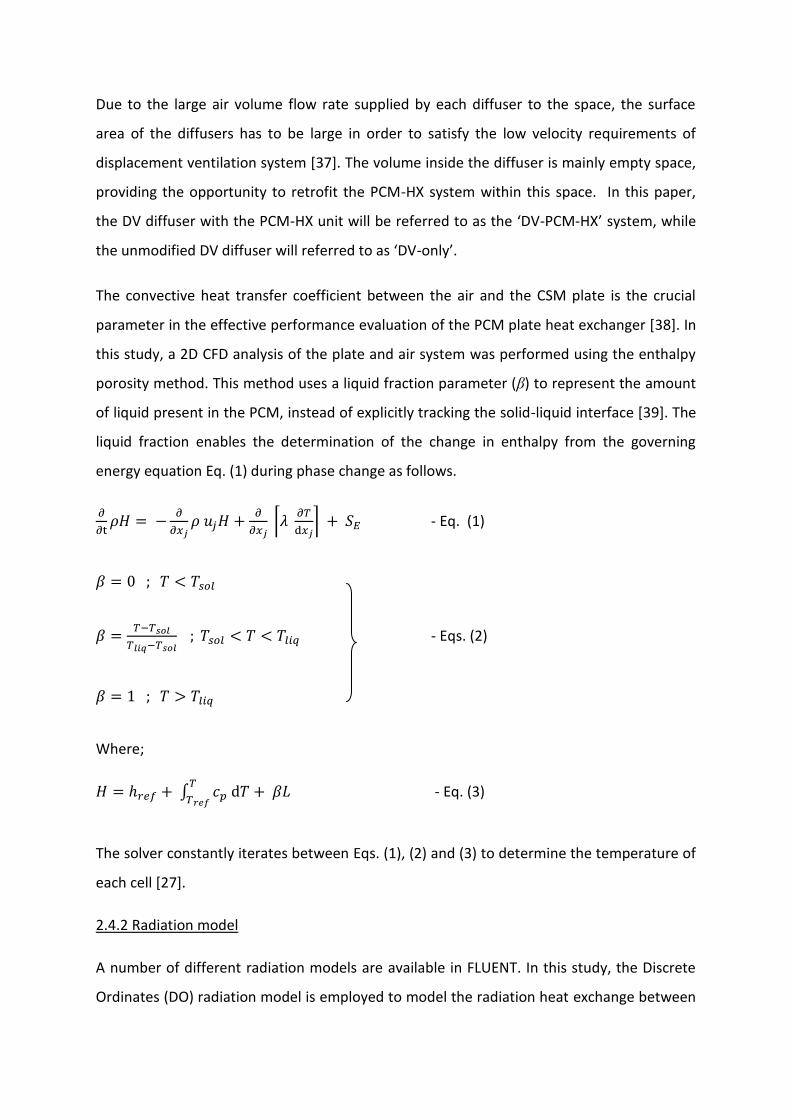
The convective heat transfer coefficient between the air and the CSM plate is the crucial

parameter in the effective performance evaluation of the PCM plate heat exchanger [38]. In

this study, a 2D CFD analysis of the plate and air system was performed using the enthalpy

porosity method. This method uses a liquid fraction parameter (β) to represent the amount

of liquid present in the PCM, instead of explicitly tracking the solid-liquid interface [39]. The

liquid fraction enables the determination of the change in enthalpy from the governing

energy equation Eq. (1) during phase change as follows.

⌈

⌉ - Eq. (1)

- Eqs. (2)

Where;

∫

- Eq. (3)

The solver constantly iterates between Eqs. (1), (2) and (3) to determine the temperature of

each cell [27].

2.4.2 Radiation model

A number of different radiation models are available in FLUENT. In this study, the Discrete

Ordinates (DO) radiation model is employed to model the radiation heat exchange between

the airport terminal building surfaces, as it is a more generic radiation model available in

FLUENT, and is more accommodating to complex geometries [33]. The model solves the

radiative heat transfer equation Eq. (4) for a finite number of discrete solid angles.

∫

All surfaces in the airport terminal building are treated as opaque and diffuse in CFD. The

effect of external solar radiation entering the space is represented by heat fluxes in the

building envelope, as described in the IEA Task 12 Report [40]. This is mainly done because

applying the solar radiation directly using the DO radiation model will result in the

inappropriate representation of long-wave radiation at night [40]. Thus, Kirchhoff’s Law is

used to account for solar load heat fluxes in the building envelope, while radiation inside the

space is considered with DO gray modelling.

The radiative heat exchange between the external surface and the sky is determined

through a fictive sky temperature, obtained from TRNSYS Type 69b. The sky energy

exchange ( , W/m2) is then obtained through Eq. (5) in FLUENT.

(

)

3.0 Model Design

3.1 TRNSYS-FLUENT Coupling strategy

Referring to the coupling methods outlined in section 2.3, a quasi-dynamic simulation is

adopted for this study. The flow of information is shown in Fig. 2.

Fig. 2. Generic flow of information in TRNSYS-FLUENT coupling

A 2D transient model of the airport was built in FLUENT. The ‘inputs’ to FLUENT at time tth,

from TRNSYS, comprise of the external weather data, heat gains and ventilation supply air

temperature, used as boundary conditions. The ‘outputs’ from FLUENT at tth are then

passed to the PID controller which controls the HVAC system. The outputs from the HVAC

system ‘updated ventilation conditions’ at t+1th are then fed back to TRNSYS for the

repetition of the cycle.

This quasi-dynamic coupling approach provides a good representation of the HVAC control

system, but requires a small enough time-step so that the switching effects of the PID

control are captured by the simulation. The time-step for the controller in TRNSYS, is based

on specifications for commercial PID temperature controllers such as the Siemens REV200®

or REV23RF®, which normally operate with switching cycles between 6 and 12 minutes,

depending on the size and thermal response of the space. The maximum time-step for the

CFD simulation was determined from an L2 norm study for temperature and velocity,

described in section 3.2.1.

3.2 Airport CFD Model

A 2D model of the airport is chosen for this study based on the constant cross-section of the

airport terminal and to reduce the simulation times to practical levels. The simulated 2D

geometry contains a fully glazed surface at the extremity, a partially glazed roof and tiled

Updated Ventilation Inputs

(t+1)th

time

Boundary conditions

tth

CFD Outputs

tth

FLUENT-

Airport

terminal

TRNSYS-

Inputs

TRNSYS -

HVAC

+Controls

Updated Ventilation Inputs

(t+1)th

time

Boundary conditions

tth

CFD Outputs

tth

floor, shown in Fig. 3. For completeness, the solid envelope domains are also discretised in

CFD to account for their thermal inertia. The glazed surfaces are externally bounded to the

ambient by convection and radiation conditions (Eq. (8)), while the floor outer surface is

adiabatic. The external convective heat transfer coefficient is taken to be 25 W/m2K, based

on the empirical ‘equation-3.6’ for hc obtained from CIBSE guide A [14] for a mean wind

speed of ~5 ms-1 at London Heathrow [41]. The external emissivity of 0.16, transmittance of

0.55 and internal emissivity of 0.2 were chosen for the external glazed surfaces based on the

specifications of commercially available structural glazing units such as ClimaGuard® [42]

and from ref. [43]. The roof transmittance is based on the assumption that it is 25% glazed,

with a fritted structure of transmittance value of 0.035 [43].

The 2D domain is supplied by a constant volume displacement diffuser, defined by a

constant mass flow rate of 0.5 kg/s, with its temperature controlled by the main AC unit in

TRNSYS. The ‘return’ is defined as an ‘outwards-mass flux inlet’ of 0.125 kg/s, to balance the

mass flow in the ducting system. Infiltration is neglected, assuming that the space is fully air-

tight. Each square (0.25 m2) mimics the internal occupancy heat gains, bounded by uniform

heat fluxes defined in Fig. 7. For the case of the actual 3D Heathrow Terminal 5, each

diffuser would serve an area equivalent to 12 times the 2D cross-section (i.e. 12m) shown in

Fig. 3, perpendicular to the drawing, with 6 kg/s air supply per diffuser. Thus, the input

boundary parameters: internal heat gains, solar heat gains and mass flow rates, are passed

from TRNSYS to the airport CFD model as heat and mass fluxes, in order to account for the

appropriate representation of the airport terminal space in 2D (with a cross-sectional

thickness of 1m).

Fig. 3. Schematic of 2D airport geometry and HVAC ducts

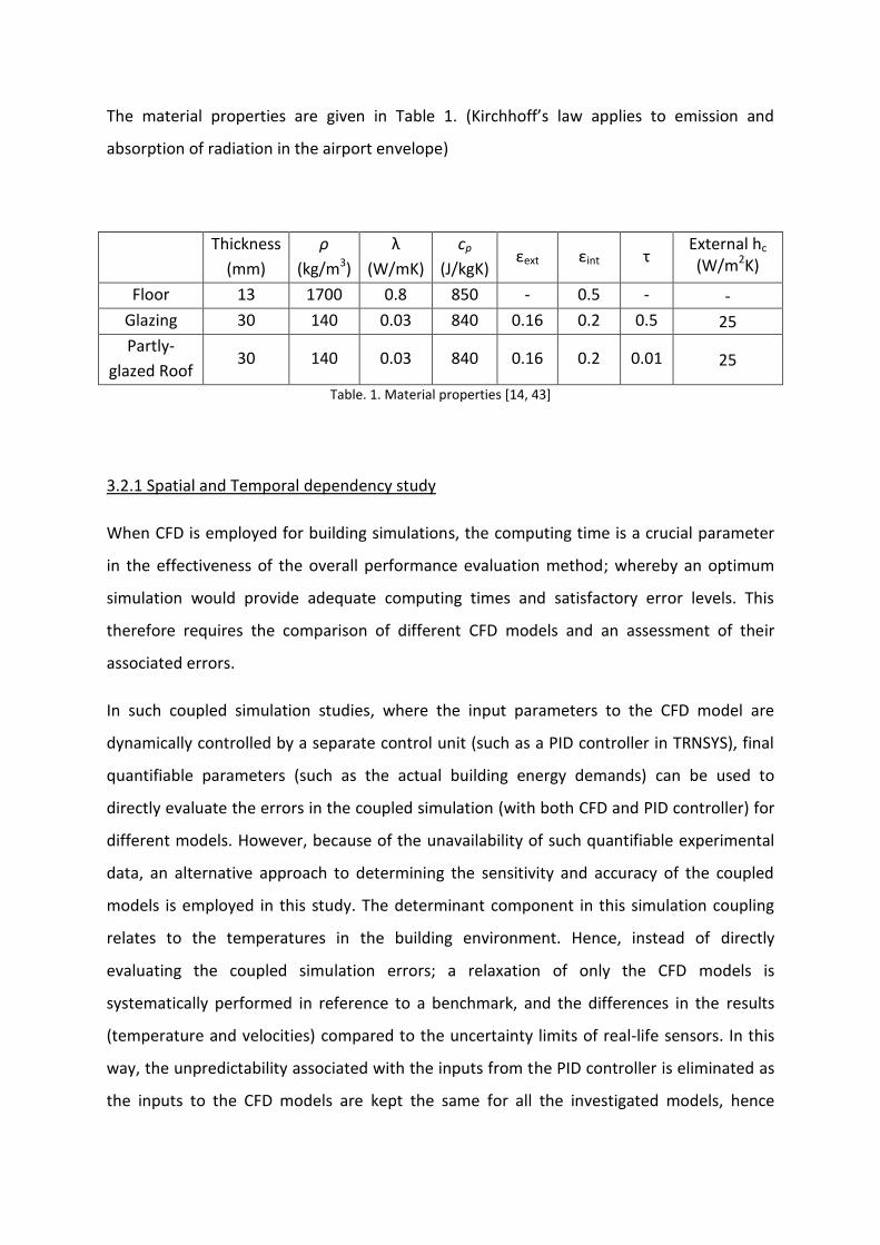
The material properties are given in Table 1. (Kirchhoff’s law applies to emission and

absorption of radiation in the airport envelope)

Thickness

(mm)

ρ

(kg/m3)

λ

(W/mK)

cp

(J/kgK) εext εint τ

External hc (W/m2K)

Floor 13 1700 0.8 850 - 0.5 - -

Glazing 30 140 0.03 840 0.16 0.2 0.5 25

Partly-

glazed Roof 30 140 0.03 840 0.16 0.2 0.01 25

Table. 1. Material properties [14, 43]

3.2.1 Spatial and Temporal dependency study

When CFD is employed for building simulations, the computing time is a crucial parameter

in the effectiveness of the overall performance evaluation method; whereby an optimum

simulation would provide adequate computing times and satisfactory error levels. This

therefore requires the comparison of different CFD models and an assessment of their

associated errors.

In such coupled simulation studies, where the input parameters to the CFD model are

dynamically controlled by a separate control unit (such as a PID controller in TRNSYS), final

quantifiable parameters (such as the actual building energy demands) can be used to

directly evaluate the errors in the coupled simulation (with both CFD and PID controller) for

different models. However, because of the unavailability of such quantifiable experimental

data, an alternative approach to determining the sensitivity and accuracy of the coupled

models is employed in this study. The determinant component in this simulation coupling

relates to the temperatures in the building environment. Hence, instead of directly

evaluating the coupled simulation errors; a relaxation of only the CFD models is

systematically performed in reference to a benchmark, and the differences in the results

(temperature and velocities) compared to the uncertainty limits of real-life sensors. In this

way, the unpredictability associated with the inputs from the PID controller is eliminated as

the inputs to the CFD models are kept the same for all the investigated models, hence

abiding to the similitude and comparative nature of error assessments. These inputs

represent typical values for airport terminal buildings [12, 43], and are shown in Fig. 4.

Thus, the errors are quantified in this study based on an L2 norm study for temperature and

velocity. The L2 norm quantifies errors based on the difference between the exact solution

of the governing differential equations and the solution of the discrete equations, as shown

by Eq. (6) [44].

L2 norm = [∑ [

]

∑ ]

- Eq. (6)

In this case, the results of a simulation with very fine-uniform mesh (307,000) and time-step

(10s) are taken as the benchmark [45]. Air is modelled as an ideal gas to account for

buoyancy effects. The body-force weighted scheme was used for the pressure discretisation,

the RNG k-ε model non-slip wall conditions were used for turbulence and the SIMPLE

algorithm was used for the pressure-velocity coupling. The enhanced wall treatment is used

to model the near-wall flows, because the enhanced-wall function in FLUENT allows an

adequate representation of the velocity and thermal profiles in the buffer region (3 < y+ <

10) [33]. This benchmark model employs the second-order discretisation scheme (as

proposed by ref. [46]), has a mean y+ value of 3.2 and a global Courant number of 1.55. The

scaled residuals resulting from this benchmark model simulation are found to be 10-4 for

continuity; 10-5 for x/y velocities, k and ε; and 10-7 for energy and DO intensity, as shown in

Fig. 5(a). The results obtained from this benchmark model were used as the basis for the

error comparisons of the different ‘relaxed’ model, as described by Eq. (6).

Fig. 4(a). External temperatures schedule input for L2 norm study

Fig. 4(b). Heat gains schedule input for L2 norm study

Fig. 4(c). Ventilation input schedule input for L2 norm study

The ‘relaxed’ models evaluated in this model independence study constitute of the

following setups: three meshes - Coarse (26,000 cells), Medium (40,000 cells) and Fine

(61,000 cells); and four time-steps - 60 s, 120 s, 360 s and 720 s. The mesh refinement was

performed by varying all mesh sizes by the same ratio, and the default FLUENT residual

convergence criteria and first-order discretisation schemes were employed for the ‘relaxed’

models. All other inputs are similar to the benchmark model. The mean errors from the L2

norm study shown in Figs. 5(b-d) are determined from 36 uniformly distributed points in the

comfort zone at heights of 0.3 m, 1.2 m, and 2 m, and time intervals of 1 hour.

Fig. 5(a). Scaled residuals for the benchmark model only, over the course of the simulation

Fig. 5(b). L2 norm for Temperature

Fig. 5(c). L2 norm for x-velocity

Fig. 5(d). L2 norm for y-velocity

The error requirements are taken to be 0.5K for the temperature values (similar to errors in

K-type thermocouples) and 0.15 m/s for the velocity values (similar to errors in the TSI

VelociCalc 8386® Pitot-tube velocity meter). Figs. 5(b-d) generally show that refining the

mesh sizes from ‘Coarse’ to ‘Fine’ gradually reduce the temperature and velocity errors for

each time-step, and that the L2 norm errors are more prominent at large time-steps. In this

regard, the velocity error requirement is satisfied with the Coarse-60s/120s, and all the

Medium and Fine configurations, whilst, the temperature error requirement is only satisfied

with the Coarse-60s/120s, Medium-60s/120s/360s and Fine-60s/120s/360s configurations.

As a result, the medium mesh with 360 s time-step was chosen for the airport CFD model,

on the basis of a temperature error level < 0.5K, velocity errors <0.15 m/s and the relatively

lower computing times.

Furthermore, although first-order discretisation schemes are used in the ‘relaxed’ models,

as opposed to second-order discretisation schemes proposed by the CFD best practice

guidelines [46], the temperature and velocity errors for the different mesh sizes and time-

steps are still within the error limits considered in this study. It should be noted that first-

order discretisation schemes are mainly used in this study due to the improved convergence

stability for the ‘relaxed’ models. Thus for the case of the simulated models, the time-steps

for both the CFD component and the controller in TRNSYS were taken to be 360s (6

minutes). It is used in TRNSYS because this time-step also suitably accounts for the PID

switching cycles described in section 3.1, and allows both TRNSYS and FLUENT to progress

with the same time-scales.

3.2.2 Grid Description

The resulting grid from the L2 norm study is shown in Fig. 6.

Fig. 6. Grid description for Airport CFD model

The mesh is designed using the in-built ANSYS® design modeller meshing algorithm, and

consists of mainly hexahedral cells. The air domain is made of unstructured mesh: with a

face cell size of 5 cm and growth rate of 1.1 at the internal gains; a face cell size of 10 cm

and growth rate of 1.05 at the envelope surfaces, producing a first inflated layer of 4 cm;

and a face cell size at the inlet and outlet of 6 cm. The mesh gradually increases towards the

bulk of the air domain producing a maximum cell size of 75 cm. The roof, glazing and floor

domains are made of structured hexahedral cells ranging from 3 cm to 10 cm, with the

finest meshes in the floor domain to appropriately account for the solar heat fluxes, defined

by Eq. (7).

It should be noted that although an actual experimental validation of the coupled simulation

would be preferred, no actual temperature measurements were available in this study.

However, the Airport CFD model errors were quantified by the L2 norm study using the

widely validated RNG k-ε turbulence model for buildings. The PCM plate model was

developed from validated works [38] and the input parameters were obtained from the

CIBSE and AHSRAE guides. The coupling strategy is similar to the validated models used in

the works of ref. [34, 36]. Furthermore, the results were used as a comparative measure

between different DV systems, rather than the characterisation of their absolute

performances in the airport terminal building.

4.0 Thermal Simulation Models

The impact of the PCM-HX system in the DV diffuser was obtained by comparing its results

to a normal DV diffuser. The following sub-sections explain the methodology employed to

evaluate the PCM-HX system and present the results. Due to extensive simulation times, the

simulations were performed for separate 100 hour intervals for discrete weather conditions

for London-UK. The annual energy results were evaluated based on the concept of Heating/

Cooling Degree Days (HDD/CDD).

4.1 Model conditions

The Meteonorm C-37790 weather files for London were used for the simulations, and the

weather data values for the 360s time-steps employed in this study are linearly interpolated

between the hourly values. The internal heat gains in the domain follow the schedule

adapted from the works of Parker et al. [12], with heat fluxes obtained from ref. [43], shown

in Fig. 7. These inputs are calculated in TRNSYS and passed as boundary conditions to the

FLUENT model, where the building is simulated.

Fig. 7. Internal heat gains schedule

Based on the radiation absorptivity for the floor of 0.5, only 50% of the solar load

transmitted by the roof and glazing is absorbed by the floor. The other 50% is assumed to be

reflected back to the outside. The heat flux on the floor due to solar radiation is therefore

obtained from Eq. 7.

[( ) ]

The heat gains at the building envelope due to ambient conditions are obtained from Eq. 8.

(

)

4.1.1 HVAC System

The AC unit is the constant air volume system shown in Fig. 3. 0.2 kg/s of fresh air [14] is

mixed with 0.3 kg/s of return air for the 2D geometry, with the ratio of fresh to return air

remaining constant. The total supply mass flow rate abides to the velocity comfort criteria

of 0.1 - 0.4 m/s in the conditioned zone from ASHRAE 55-2004 [47].

In the actual diffuser shown in Fig. 1(b), the total mass flow rate would be 12 times that of

the 2D geometry (equivalent to the total area served by one diffuser), i.e. 6 kg/s. The PID

controller respectively adjusts the amount of cooling and heating provided based on the

temperature feedback (Tf), from a sensor located at an important location in the passenger

0

10

20

30

40

50

60

70

80

0 1 2 3 4 5 6 7 8 9 10 11 12 13 14 15 16 17 18 19 20 21 22 23 24

Hea

t G

ain

s (W

/m2)

Time of Day (hr)

Internal Heat gains

zone [15] as shown in Fig. 3. As a result, the TRNSYS HVAC component adjusts the diffuser

inlet temperature in FLUENT, for each time-step, as shown in Fig. 8.

Fig. 8. Schematic of AC unit

A comfort temperature range of 18-23 oC [14] was used with the PID controller; calling for

heating/cooling if Tf is outside this temperature range. Within the comfort temperature

range, the supply temperature Ts is equal to the mixed temperature Tm in the DV-only case,

or the PCM-conditioned temperature in the DV-PCM-HX case, in order to portray the free-

conditioning potential of the space and to reduce energy consumption. The PID set point

temperature is 21 °C, and the integral, derivative and gain constants are 0.1 hour, 0.1 hour

and 10% respectively. The PID set point temperature is maintained constant for all seasons,

as it can be considered a mean optimum thermal comfort temperature condition [48]. This

was verified for the case of an airport terminal space in the UK, based on: 1.15 clo, 1.4 met

and air velocity of 0.15 ms-1 for winter conditions; and 0.65 clo, 1.4 met and air velocity of

0.15 ms-1 for summer conditions [14]; whereby a temperature of 21 °C is found to provide

an adequate PMV of ±0.5 for the occupants in both seasons, using the Fanger’s equation of

thermal comfort [49].

The capacity of the terminal heating and cooling units was assumed to be 4 kW each,

producing a maximum air ΔT of 8 K across the units, with a constant mass flow rate of 0.5

kg/s. These parameters were maintained for both the DV-only and the DV-PCM-HX

simulations. The AC unit was assumed to be operational during the occupied hours between

04:00 and 24:00. During the non-occupied hours for the DV-only case, the AC system was

assumed to be shut down with no external air entering the space. For the DV-PCM-HX

system case, different PCM night charging strategies were investigated.

- +

AIRPORT

DOMAIN

IN FLUENT

PID

Tm Ts

Tr

Tamb

Texh

Tf

Ts

Tr

Tamb

Texh

4.2 Case of DV-only system - Results

Due to extensive simulation times, three discrete weather conditions were used to evaluate

the performance of the DV systems: summer, intermediate and winter. All simulations were

initialised at the optimum comfort temperature of 21 oC, and the results are depicted in Fig.

9. A time-step of 360 s with an average of 40 iterations per time-step was employed for the

CFD simulation. The overall actual simulation time for each season was 13 hours with a

3GHz i7 processor.

Fig. 9(a). Zone temperature (Tf) profiles for three distinct seasons in ‘DV-only’ Case

Fig. 9(b). Heating (+ve) and Cooling (-ve) Load on AC unit in ‘DV-only’ case for 2D geometry

During the intermediate period, the AC unit successfully controls Tf within the comfort

temperature range of 18-23 oC. The majority of the energy requirement is for cooling, with a

relatively small amount for heating during the early hours of the morning. During the

summer period, the zone temperature is less effectively controlled compared to the

intermediate season, where the temperature reaches ≈26oC at mid-day. Similar to the

intermediate season, the majority of the load is for cooling, but heating is also required on a

small number of occasions when the ambient temperature is low during the early morning.

During winter, only heating is required. However, Fig. 9(a) shows that based on the control

strategy used, the AC unit is unable to satisfy the comfort requirements in winter and the

zone temperature varies between 15 oC and 18oC.

Fig. 10(a). Temperature contour (

oC) still-frame during the AC unit cooling mode

Fig. 10(b). Temperature contour (

oC) still-frame during the AC unit heating mode

Fig. 10 further demonstrates why DV is more suitable for cooling, rather than heating large

spaces. During the cooling mode (Fig. 10(a)), the buoyancy effects of the DV system enhance

cooling in the space as the cold air spreads on the floor until it reaches a heat source. This

enables the cooling potential of the system to be specifically directed to the occupied space,

and avoid unnecessary conditioning of unoccupied areas. Furthermore, the temperature

stratification effect in the space prevents further heat gains from the higher level in the

building envelope by reducing the temperature difference with the external conditions. In

the case of heating, the DV system behaviour resembles a mixed ventilation system. Fig.

10(b) shows that the warm air supplied by the displacement diffuser due to the dominant

buoyancy effects rises very quickly and mixes with the air in the space, failing to establish

temperature stratification in the space.

4.3 Case of DV-PCM-HX system

The PCM heat exchanger (PCM-HX) is accommodated inside the DV diffuser, at the end of

the air-conditioning duct, just before the supply into the airport space, as shown in Fig. 1(c).

As a result, the control of the system becomes more complex due to the uncertainty in

supply temperature (Ts) as the air passes through the PCM. The control system is therefore

slightly modified to allow for the conditioned air to only pass through the PCM-HX when the

zone temperature is within comfort; 18 oC < Tf < 23 oC. For conditions where Tf is outside the

comfort range, the conditioned air from the heating/cooling unit bypasses the PCM-HX unit,

and directly enters into the airport space, as depicted in Fig. 1(c). This concept maintains

‘free-conditioning’ of the space with PCM-HX used only when Tf is within comfort.

4.3.1 PCM-HX simulation model

As mentioned in section 2.4.1, due to the different interactions in this system, the PCM-HX

is also simulated in FLUENT. This is done through a separate custom-built TRNSYS

component that links the appropriate inputs to FLUENT, resulting in a secondary quasi-

dynamic coupling within the same simulation. The flow of information between TRNSYS and

FLUENT is thus modified as shown in Fig. 11.

Fig. 11. Modified information flow for DV with PCM-HX

Owing to the successive substitution method in TRNSYS, the components are solved

sequentially, such that the simulation time for each TRNSYS-FLUENT coupled component is

additive.

Due to the symmetrical nature of the PCM-HX system, a 2D CFD model for the CSM plate

arrangement is employed (Fig. 12(a)). The protrusions of the plate surface into the air

stream, shown in Fig.1(a), is incorporated in the simulations as a surface roughness of 0.25

mm [38]. In addition to the ‘boundary conditions-1’ employed in the section 3.1, the

‘boundary conditions-2’, referred to in Fig. 11, are also employed and comprise of the inlet

air mass flow rate and temperature to the PCM plate. ‘CFD output-2’ are the air

temperature exiting the PCM-HX and the PCM mean temperature.

The mesh employed in the CSM plate model consists of structured 1*3mm hexahedral cells

in the PCM domain, and hexahedral cells with a face size of 2mm with growth ratio of 1.2 in

the air domain, as shown in Fig. 12(a). The RNG k-ε turbulence model was used as it is

adaptable to both high and low turbulence scenarios [50]. The phase change process was

modelled with the enthalpy porosity method. The properties of the PCM used are: λ = 0.2

W/mK; ρ = 820 kg/m3; cp = 2100 J/kgK; phase change range = 16 - 25 oC; and latent enthalpy

= 180 kJ/kg.

To allow for appropriate residual convergence, a time-step of 20 s was employed. Hence, for

one time-step in the FLUENT Airport and TRNSYS models, 18 sub time-steps were performed

for the PCM plate to ensure that all the simulation components were at the same time.

FLUENT:

Airport

terminal

FLUENT:

PCM-HX

TRNSYS- Inputs

TRNSYS -

HVAC +

Controls

tth

Boundary

Conditions -2

Updated Ventilation Inputs

(t+1)th

time

CFD Outputs -2

tth

Boundary Conditions-1

tth

CFD Outputs -1

tth

Fig. 12(a) Model description of CSM Plate

Fig. 12(b). Heat transfer rates of PCM-HX unit for different air-gaps between plates at a total mass flow rate of

6 kg/s (i.e. 0.5 kg/s/m in 2D *12m served by 1 diffuser). ΔT is the temperature difference between the incoming air and the PCM plate.

Considering the results in Fig. 9(b), the average load on one DV diffuser over the three

seasons was found to be 32 kW (i.e. 12 × average load from Fig. 9(b)). Hence, based on the

data from Fig. 12(b), obtained from the simulation of the model in Fig. 12(a), an air gap of 16

mm between the PCM plates was used. This produces a maximum heat transfer rate

equivalent to the 32 kW capacity required by the DV system at a ΔT of 7 K. This amounts to

125 rows, with 12 CSM plates in each row, uniformly arranged as shown in Fig. 1(c),

resulting in a mass flow rate of 0.048 kg/s per row and a total latent energy of 133 MJ for

one diffuser. At this mass flow rate, the static pressure drop across the PCM plates is 10 Pa

with a heat transfer coefficient of 14.3 W/m2K, obtained using the CFD model described in

Fig. 12(a). Although this sizing method is relatively simple and assumes that the air reaches

the PCM temperature at the PCM-HX outlet, it only serves as an approximation for system

sizing. The actual performance is evaluated in the following sections.

4.3.2 DV-PCM-HX Charging Strategy

As elaborated in various studies [1-5], the energy stored when the PCM is charged, has to be

discharged in order to allow the appropriate and repetitive functioning of the energy

storage system. The most common PCM charging method involves passing cold night air to

solidify the PCM and restore its cooling potential.

In this study, three different charging strategies are investigated when the airport terminal

building is closed between 24:00 and 04:00 as follows: i) no night ventilation; ii) non-stop

full ventilation; and iii) a limiting ventilation control. During the intermediate and summer

periods, cold ambient air is used for charging. The limiting control is done by monitoring the

PCM temperature, and ending night ventilation when the PCM temperature drops below 18

oC, the lower comfort level. During the winter period, the return air from the airport is re-

circulated through the PCM-HX to store the extra heat from the space. In this case, the

limiting control is performed by monitoring the difference between the return air

temperature and the PCM temperature, such that night ventilation is active only when there

is a net positive heat transfer into the PCM.

4.3.3 DV-PCM-HX system – Results

Similar to the DV-only case, three discrete weather conditions were used for performance

evaluation of the DV-PCM-HX system. The time-step used was 360 s, with an average of 40

iterations per CFD time-step. The overall total simulation time for each season was 19 hours.

Fig. 13(a). Zone temperature (Tf) profiles for three distinct seasons in ‘DV-PCM-HX’ Case

Fig. 13(b). Heating (+ve) and Cooling (-ve) Load on AC unit in ‘DV-PCM-HX’ case for 2D geometry

Fig. 13 shows the behaviour of the DV-PCM-HX system to be similar to the DV-only system.

The DV-PCM-HX system is able to satisfy the comfort conditions only during the

intermediate season. There is slight overheating during the summer, whilst the temperature

during the winter drops outside the comfort region. With regards to energy demand, it can

be seen that full ventilation control increases the heating demand during both the

intermediate and summer periods due to space over-cooling, relative to the other

strategies. The winter heating loads are similar for all control strategies. The overall

temperature progression of the three control strategies is very similar.

During the intermediate and summer season, Tf and Tamb fluctuate within the PCM phase

change range, while during the winter, Tf tends to stay below the lower limit of the phase

change range. This accounts for the varying impact of the control strategy on the energy

demand. A detailed comparison between the DV-only and the DV-PCM-HX cases are given in

section 4.4.1.

4.4 Yearly energy demand

4.4.1 Heating / cooling energy demand

The yearly thermal energy demand was determined using the Heating and Cooling Degree

days (HDD/CDD) concept, as proposed by CIBSE TM-41 [51]. Degree days are a measure of

how much (in degrees), and for how long (in days), the external air temperature was lower

than a specific base temperature in the case of heating or above a specific base temperature

in the case of cooling. They are used for calculations relating to the energy required to heat

or cool buildings [52, 53].

The base temperatures were obtained from the results of the DV-only case in Fig. 9(a) for

the intermediate season, where the heating and cooling demands are relatively uniform. It

can be observed that heating is required when the ambient temperature is below 15 oC,

while cooling is required for ambient temperatures above 18 oC. These two temperatures

were thus taken as the base temperatures for HDD and CDD, respectively.

Seasons HDD CDD

Simulated Winter 46.35 0.00

Simulated Summer 0.29 13.79

Simulated Intermediate 2.49 6.27

Entire Year 1859.12 120.10

Table. 2. Simulated and yearly Degree days for 15oC and 18oC base temperatures

Due to extensive computing times, the simulations were run for 100 hours in each typical

summer, winter and intermediate conditions. The HDD and CDD for these three periods in

Table 2 therefore refer to the individually simulated 100 hours. The total HDD and CDD for

the entire year are then used to extrapolate for the yearly energy demand based on these

typical simulated conditions. The limitations of such extrapolation concepts have been

identified in ref. [51], however HDD and CDD have been employed in several studies in the

prediction of building energy consumption [52, 53]. This is due to its simplicity and speed of

use, as well as the possibility to easily estimate the building performance for different

weather conditions. This concept is hence adopted as an adequate design estimation option

for simulations requiring long computing times.

Fig. 14. HVAC energy demand per Degree Day (DD) over the three simulated seasons for different DV

configurations (+ve is heating demand)

In order to avoid initialisation errors, the first day of the simulations was not included in the

energy analysis. Fig. 14 shows that the addition of the PCM-HX in the DV diffuser has a

greater effect on the heating energy requirement than the cooling energy requirement. It

can be seen that reducing night ventilation to charge the PCM, reduces the heat demand in

the intermediate and summer periods as overcooling in the morning is reduced. The use of

the PCM-HX has little effect on the heating demand in winter, due to the fact that the

temperature of the air (Tm or Tr) passing through the PCM-HX is lower than the PCM phase

change temperature range of 16-26 °C, as shown in Fig. 13(a). The latent storage capacity of

the PCM is therefore inefficiently used during winter.

On the other hand, the cooling demand in both the summer and intermediate periods are

reduced with the addition of the PCM-HX, relative to the DV-only system. However the

different ventilation charging strategies do not affect the performance. Previous studies

have primarily shown that PCM systems can reduce cooling demand or temperature swing

in intermittently occupied buildings [1-6]. However, as the airport schedule is less uniform

and different to intermittently occupied buildings, this study shows that the PCM-HX has a

higher impact on the heating demand of the space during the intermediate and summer

periods.

Fig. 15(a). Zone temperatures (Tf) and PCM temperatures during one day in the Intermediate period

Fig. 15(b). Heating (+ve) and cooling (-ve) energy demand for one day in the intermediate period

Fig. 15(a) shows that during the early hours of the morning, the zone temperature is less

than the lower comfort limit of 18oC, with the space requiring heating. Employing a full

ventilation charging strategy implies that the temperature being supplied to the space from

the PCM-HX is lower compared to the other configurations, hence increasing the heating

requirement. Preventing night ventilation or limiting the PCM temperature to 18oC will

reduce the need for heating in the early hours (at 4564 hr) of the morning. Fig. 15(b) shows

that the use of the PCM-HX shifts the occurrence of high space temperature from the

morning hours towards mid-day, reducing cooling energy requirements in the morning. The

overall cooling energy requirement of the space is also reduced with the use of the PCM-HX.

4.4.2 Pressure Drop Calculations

The different ventilation configurations studied in this paper have an impact on the air

pressure drop in the system and energy consumption. To determine the effect of pressure

drop in the different ventilation strategies, the system boundary in Fig. 3 was used for the

calculations.

The sizing of the ducts was based on the velocity criteria provided by CIBSE [37] and

equations given in ref. [54] assuming a constant air volume system. A velocity of 15 m/s was

used for the main ducts giving a diameter of 0.65 m and a velocity of 10 m/s with a duct

diameter of 0.45 m for the final duct run to the diffuser. The pressure drop across the PCM-

HX was 10 Pa, as discussed in section 4.3.1.

4.4.3 Total yearly energy demand

The total energy demand of the space is the sum of the thermal energy requirement of the

HVAC system and the energy consumption of the fans to overcome pressure losses. For this

case study, 24 DV diffusers were present in the airport terminal building.

Fig. 16. Total yearly energy demand for the entire airport departure hall

The total annual energy consumption of the conventional DV system and the DV-PCM-HX is

shown in Fig. 16. It can be seen that when no night ventilation and limiting control

ventilation strategies are used, the DV-PCM-HX system can result in 34% and 22% energy

savings, respectively, compared to the conventional DV system. The full night ventilation

strategy for the DV-PCM-HX system will result in 20% higher energy consumption compared

to the DV-only system. This higher energy results from higher HVAC energy due to

overcooling of the space and higher fan power.

5.0 Conclusions

This study evaluates the energy impact of a PCM-HX retrofitted into an airport DV diffuser.

The evaluation was performed using a TRNSYS-CFD coupled simulation and comparing the

energy demands of a DV-only system with that of a DV-PCM-HX system under different

charging strategies for the PCM. The results show that:

displacement ventilation is more appropriate for cooling rather than heating

applications as it relies on buoyancy effects to provide stratification and reduce the

volume of air in the space that needs to be cooled compared to mixing HVAC

systems.

the addition of the PCM-HX in the DV diffuser reduces the energy requirement for

heating in the intermediate and summer periods when ‘no-night-ventilation’ and

‘limiting-control-ventilation’ night charging strategies for the PCM are used. These

PCM charging strategies lead to annual energy demand reductions for the airport

terminal building of 1060 MWh (34%) or 680 MWh (22%), respectively. During

winter, the DV-PCM-HX system does not have much effect as the zone temperature

during the unoccupied hours can fall outside the phase change temperature range of

the PCM.

during the intermediate and summer seasons, the DV-PCM-HX shifts the cooling load

from the early hours in the morning to later in the day and reduces the overall HVAC

energy requirement for cooling compared to the DV-only system.

Further work will consider the effect of a wider comfort temperature band, more

sophisticated control strategies and alternative PCM-HX configurations.

6.0 Acknowledgements

This work was made possible through sponsorship from the UK Engineering and Physical

Sciences Research Council (EPSRC), Grant No: EP/H004181/1. The TRNSYS Fortran

debugging process was facilitated by D. Bradley of Thermal Energy Systems Specialists

(TESS-inc), Madison, Wisconsin.

7.0 REFERENCES:

[1] Y. Zhang, G. Zhou, K. Lin, Q. Zhang, H. Di, Application of latent heat thermal energy storage in

buildings: State-of-the-art and outlook, Building and Environment 42(2011), pp. 2197-2209.

[2] B. Zalba, J.M. Marin, L.F. Cabeza, H. Mehling, Free-cooling of buildings with phase change

materials, International Journal of Refrigeration, 27(2004), pp. 839-849.

[3] D. Zhou, C.Y. Zhao, Y. Tian, Review on thermal energy storage with phase change materials

(PCMs) in building applications, Applied Energy 92(2012), pp. 593-605.

[4] P. Arce, C. Castellon, A. Castell, L.F. Cabeza, Use of microencapsulated PCM in buildings and the

effect of adding awnings, Energy and Buildings 44(2012), pp. 88-93.

[5] G. Susman, Z. Dehouche, T. Cheechern, S. Craig, Tests of prototype PCM ‘sails’ for office cooling,

Applied Thermal Engineering 31(2011), pp. 717-726.

[6] L. Shilei, F. Guohui, Z. Neng, D. Li, Experimental study and evaluation of latent heat storage in

phase change materials wallboards, Energy and Buildings 39(2007), pp. 1088-1091.

[7] E. Osterman, V.V. Tyagi, V. Butala, N.A. Rahim, U. Stritih. Review of PCM based cooling

technologies for buildings, Energy and Buildings 49(2012), pp. 37-49

[8] C. Arkar, B. Vidrih, S. Medved, Efficiency of free cooling using latent heat storage integrated into

the ventilation system of a low energy building, International Journal of Refrigeration 30(2007), pp.

134–143

[9] N.H.S Tay, M. Belusko, F. Bruno. Designing a PCM storage system using the effectiveness-number

of transfer units method in low energy cooling of buildings, Energy and Buildings 50(2012), pp. 234-

242

[10] http://www.monodraught.com , Accessed on 22 December 2012

[11] http://www.troxtechnik.com , Accessed on 22 December 2012

[12] J. Parker, P. Cropper, L. Shao. Using building simulation to evaluate low carbon refurbishment

options for airport buildings, Proceedings of Building Simulation 2011: 12th Conference of

International Building Performance Simulation Association, Sydney, 14-16 November 2011, pp. 554-

561.

[13] P. Simmonds, W. Gaw. Using a constant volume displacement ventilation system to create a

micro climate in a large airport terminal in Bangkok, Proceedings of the Tenth Symposium on

Improving Building Systems in Hot and Humid Climates, Fort Worth, TX, May 13-14, 1996, pp. 217-

227

[14] Chartered Institute of Building Services Engineering, Guide A (2006).

[15] J. Liu, N. Yu, B. Lei, X. Rong, L. Yang. Research on indoor environment for the terminal 1 of

Chengdu Shuangliu International airport, Proceedings of the Eleventh International IBPSA

Conference, Glasgow, Scotland, 27-30 July 2009.

[16] http://www.rsh-p.com , Accessed on 22 December 2012

[17] H. Goodfellow, E. Tahti. Industrial ventilation design guidebook. 1st Edition, Academic Press;

2001

[18] H.B. Awbi, Energy efficient room air distribution, Renewable Energy 15 (1998), pp. 293-299.

[19] D.B. Crawley, J.W. Hand, M. Kummert, B. T. Griffith, Contrasting the capabilities of building

energy performance simulation programs, Building and Environment 43(2008), pp. 661–673.

[20] http://www.iesve.com/news , Accessed on 22 December 2012

[21] http://www.designbuilder.co.uk/content/view/40/61/ , Accessed on 22 December 2012

[22] TRNSYS-17 manual, Volume 1: Getting Started, 2009

[23] M. Matsuia, H. Takayanagi, Y. Oda, K. Komurasaki, Y. Arakawa, Performance of arc jet-type

atomic-oxygen generator by laser absorption spectroscopy and CFD analysis, Vacuum 73(2004), pp.

341-346.

[24] M. Tye-Gingras, L. Gosselin, Comfort and energy consumption of hydronic heating radiant

ceilings and walls based on CFD analysis, Building and Environment 54(2012), pp. 1- 13.

[25] P. Gousseau, B. Blocken, T. Stathopoulos, G.J.F. van Heijst, CFD simulation of near-field

pollutant dispersion on a high-resolution grid: A case study by LES and RANS for a building group in

downtown Montreal, Atmospheric Environment 45(2011), pp. 428-438.

[26] Zhang, Z., Zhang, W., Zhai, Z., and Chen, Q.Y., Evaluation of various turbulence models in

predicting airflow and turbulence in enclosed environments by CFD: Part-2 - comparison with

experimental data from literature, HVAC&R Research 13(2007), pp. 871-886.

[27] K.G. Gebremedhin, B.X. Wu, Characterization of flow field in a ventilated space and simulation

of heat exchange between cows and their environment, Journal of Thermal Biology, 28 (2003), pp.

301–319.

[28] P. Rohdin, B. Moshfegh, Numerical predictions of indoor climate in large industrial premises. A

comparison between different k-ε models supported by field measurements, Building and

Environment 42(2007), pp. 3872-3882.

[29] S. Hussain, P.H. Oosthuizen, A. Kalendar, Evaluation of various turbulence models for the

prediction of the airflow and temperature distributions in atria, Energy and Buildings 48(2012), pp.

18-28.

[30] Z. Zhai, Z. Zhang, W. Zhang, Q.Y. Chen, Evaluation of various turbulence models in predicting air

airflow and turbulence in enclosed environments by CFD. Part-1: Summary of prevent turbulence

models, HVAC and R Research 13 (2007), pp. 853-870

[31] S. Leenknegt, R. Wagemakers, W. Bosschaerts, D. Saelens, Numerical sensitivity study of

transient surface convection during night cooling, Energy and Buildings 53(2012), pp. 85-95.

[32] B.L. Gowreesunker, S.A. Tassou. Effectiveness of CFD simulation for the performance prediction

of phase change building boards in the thermal environment control of indoor spaces, Building and

Environment 59(2013), pp. 612-625.

[33] ANSYS FLUENT Theory Guide; Nov 2010. Release 13.0.

[34] Z.J. Zhai, Q.Y. Chen. Performance of coupled building energy and CFD simulations, Energy and

Buildings 37(2005), pp. 333-344.

[35] D.A. Arias, Advances on the coupling between a commercial CFD package and a component-

based simulation program, Second National IBPSA-USA Conference (SimBuild 2006), Cambridge, MA,

August 2-4, 2006.

[36] Y. Fan, K. Ito. Energy consumption analysis intended for real office space with energy recovery

ventilator by integrating BES and CFD approaches, Building and Environment 52(2012), pp. 57-67.

[37] Chartered Institute of Building Services Engineering, Guide B (2006).

[38] P. Dolado, A. Lazaro, J.M. Marin, B. Zalba, Characterization of melting and solidification in a real

scale PCM-air heat exchanger: Numerical model and experimental validation, Energy Conversion and

Management 52(2011), pp. 1890-1907.

[39] V. R. Voller and C. R. Swaminathan, Generalized Source-Based Method for Solidification Phase

Change, Numerical Heat Transfer, Part B 19(1991): pp. 175-189.

[40] I. Bryn, P.A. Schiefloe, Atrium models for the analysis of thermal comfort and energy use, A

report of the International Energy Agency (IEA) Task 12 – Building Energy analysis and design tools

for solar applications, Project A.3, March 2006.

[41] https://restats.decc.gov.uk/cms/annual-mean-wind-speed-map , Accessed on 14 March 2013

[42] http://www.guardianglass.co.uk/architectural/product/detail/climaguard-aplus , Accessed on

14 Mar 2013

[43] P. Simmonds, S. Holst, S. Reuss. Using radiant cooled floors to condition large spaces and

maintain comfort conditions, ASHRAE Transactions 106 (2000), pp. 695–701.

[44] Veluri SP, Roy CJ, Luke EA, Comprehensive Code Verification Techniques for Finite Volume CFD

Codes, Computers & Fluids (2012), doi: http://dx.doi.org/10.1016/j.compfluid.2012.04.028 .

[45] Alauzet F, Frey PJ, George PL, Mohammadi B. 3D transient fixed point mesh adaptation for time-

dependent problems: Application to CFD simulations, Journal of Computational Physics 222(2007),

pp. 592–623.

[46] R. Ramponi, B. Blocken, CFD simulation of cross-ventilation for a generic isolated building:

Impact of computational parameters, Building and Environment 53 (2012), pp. 34–48.

[47] ASHRAE Standard 55-2004, Thermal Environmental Conditions for Human occupancy (2004).

[48]A. Auliciems, S.V. Szokolay. Thermal comfort: Passive and low energy Architecture International

design tools and techniques, PLEA Note 3. ISBN: 0867767294. 2nd Edition. The University of

Queensland; 2007

[49] P.O. Fanger. Thermal comfort: Analysis and applications in environmental engineering. McGraw-

Hill Book Company; 1970.

[50] P. Rohdin, B. Moshfegh. Numerical predictions of indoor climate in large industrial premises. A

comparison between different k-ε models supported by field measurements, Building and

Environment 42(2007), pp. 3872-3882

[51] T. Day. Degree days: Theory and Applications, CIBSE TM-41, 2006.

[52] M. Kolokotroni, M. Davies, B. Croxford, S. Bhuiyan, A. Mavrogianni. A validated methodology for

the prediction of of heating and cooling energy demand for buildings with the Urban Heat Island:

Case-study of London, Solar Energy 84(2010), pp. 2246-2255.

[53] A. Bolatturk. Optimum insulation thickness for building walls with respect to cooling and

heating degree-hours in the warmest zone of Turkey, Building and Environment 43(2008), pp. 1055-

1064.

[54] I.E. Idelchik. Handbook of hydraulic resistance. 3rd Edition. CRC Press; 1994.