coupled simulation of indoor environment, hvac...

2014 ASHRAE/IBPSA-USA Building Simulation Conference

Atlanta, GA September 10-12, 2014

COUPLED SIMULATION OF INDOOR ENVIRONMENT, HVAC AND CONTROL

SYSTEM BY USING FAST FLUID DYNAMICS AND THE MODELICA BUILDINGS LIBRARY

Wangda Zuo1,*, Michael Wetter2, Dan Li1, Mingang Jin3, Wei Tian1, Qingyan Chen3 1University of Miami, Coral Gables, FL

2Lawrence Berkeley National Laboratory, Berkeley, CA 3Purdue University, West Lafayette, IN

*Corresponding Author: [email protected]

ABSTRACT

Ventilations with stratified air distributions are commonly used to reduce building energy consumption while improving the indoor environment quality. This paper describes the coupling of transient simulations of indoor environments with HVAC systems, controls and building envelope. The indoor environment was simulated using a fast fluid dynamics (FFD) simulation program. The building fabric heat transfer, HVAC and control system were modeled using the Modelica Buildings library. After presenting the concept, the mathematical algorithm and the implementation of the coupled simulation, two numerical examples of ventilation with natural convection and mixed convection in a single-room building are provided for validation and demonstration. Further research and development needs are also discussed.

INTRODUCTION Ventilations with stratified air distributions are commonly used to reduce building energy consumption while improving the indoor environment quality. Examples include displacement ventilation and hybrid ventilation. To optimize the design and control of these buildings’ HVAC systems, a coupled simulation of the indoor environment and the HVAC system is needed. In the past, coupled simulations between building energy simulation tools and computational fluid dynamics (CFD) were proposed to study the energy performance for buildings with stratified air distributions (Zhai et al., 2002, Djunaedy et al., 2005). Due to the long computation time required by the CFD, most coupled simulations usually perform only a few steady-state CFD simulations to compute the critical indoor environment information for the building energy simulation. These previous coupled simulations used conventional building energy simulation programs and CFD tools that were sufficient for estimating building energy performance. However, using only a few steady-state CFD simulations is not appropriate for the design and optimization of an HVAC control for a stratified

indoor environment as it does not account for the dynamics of the feedback control. Furthermore, conventional building simulation tools, such as EnergyPlus, are designed for whole building energy performance simulations and implement idealized control, often embedded in equipment models.

The purpose of this research is to develop a coupled simulation of an indoor environment and a building HVAC system that can simulate the transient interaction between room air flow, HVAC, building envelop and feedback control. For the indoor environment simulation, the Fast Fluid Dynamics (FFD) program (Zuo et al., 2009, Jin et al., 2012b), written in the C language, was selected. FFD solves the same Navier-Stokes equation and other governing equations as CFD. However, by employing different numerical algorithms and sacrificing some accuracy, FFD simulations have been shown to be around 50 times faster than their CFD counterparts. In addition, parallel computing on a graphics processing unit further accelerates the FFD (30 times faster). Consequently, this results in a total speedup of 1,500 times faster than CFD (Zuo et al., 2010a). The FFD program was used to study various airflows inside and around buildings (Zuo et al., 2010c, Zuo et al., 2010b, Jin et al., 2013b, Jin et al., 2013a, Jin et al., 2012a). The building envelope and HVAC system are modeled using the Modelica Buildings library (Wetter et al., 2014). Modelica is an equation-based, object-oriented modeling language for the simulation of multi-domain dynamic systems. The Buildings library is an open-source, freely available Modelica library for building energy and control systems. It has been used for the design and performance evaluation of various buildings’ energy and control systems (Kim et al., 2013, Ansuini et al., 2012, Zuo et al., 2011).

This paper is structured as follows: The next section discusses the mathematical algorithm for the coupled simulation between FFD and the Modelica Buildings library. Afterwards, the implementation of the FFD programs and Modelica models is discussed. Next, the

© 2014 ASHRAE (www.ashrae.org). For personal use only. Reproduction, distribution, or transmission in either print or digital form is not permitted without ASHRAE’s prior written permission.

56

implementation is validated quantitatively using ventilation with natural convection, and qualitatively using ventilation with mixed convection. Finally, further research and development needs are discussed at the end of the paper.

DATA EXCHANGE ALGORITHM This section describes the algorithms that conduct the data exchange between the FFD and Modelica models. This differs from coupling the CFD and conventional building energy simulation programs. The major challenge of coupling the FFD and Modelica models is the data exchange between the causal input/output signal flow semantics of FFD and the acausal semantics of Modelica models. Because of the similarity of FFD and CFD, the mathematical algorithms discussed in this section can also be used for future coupling between CFD and Modelica models.

Fluid Ports

In the Modelica Buildings library, the fluid flow into and out of models is simulated with fluid ports. These ports carry variables for pressure, mass flow rate, enthalpy, mass fractions (such as for water vapor) and optional trace substances (such as carbon dioxide) that are carried by the mass flow. The fluid ports in the Modelica model correspond to the inlet and outlet boundaries in the FFD. The direction of the mass flow rate can be reversed in Modelica as needed to satisfy the pressure and flow equations. Therefore, in the FFD program, air inlets or outlets need to be assigned by checking the direction of the mass flow rate. This is done using the following rules: If the flow goes into the room space, then the fluid port is an inlet, otherwise it is an outlet.

For the “inlet” fluid port, the Modelica model calculates the inlet boundary conditions for FFD. At the time of the data exchange, , the FFD program converts the inlet averaged airflow rate obtained from Modelica to the inlet velocity . FFD then assumes a uniform velocity distribution on the inlet surface. Hence

1, (1)

where is the fluid density and is the inlet surface area, and is the time interval between two data exchanges. In addition, Modelica defines the temperature, concentration of species, and trace substances at the inlet by using their corresponding quantities at the fluid port.

For the “outlet” fluid port, the Modelica model will receive the boundary conditions from FFD. FFD computes the time averaged mass flow rate as

, , (2)

where , is the velocity normal to the mesh surface s at the outlet and is the total surface area of the outlet. The time averaged air temperature at the outlet, , is computed as

, , , (3)

where , is the air temperature on the mesh surface. Other scalar variables, such as mass fraction and trace substances concentration, are calculated similarly.

Walls and Windows

For the FFD simulation, thermal boundary conditions of solid surfaces, such as walls and windows, can either have a given temperature or a given heat flux. In the current implementation, if Modelica provides to FFD the temperature of an average solid surface as

1, (4)

then FFD will compute the heat flux accordingly and provide Modelica the heat flow rate as

1, , (5)

where , is the heat flux through the solid surface s.

Alternatively, if Modelica computes the averaged heat flow rate as

1,

(6)

then FFD converts it to a heat flux as

. (7)

Similarly, FFD then computes the mean temperature as

1 1, . (8)

Other Variables

For internal heat sources, the current implementation assumes the heat flow rate , injected into the


57

space, to be uniformly distributed. Hence, the heat flow rate in FFD is

, (9)

where V is the volume of the room air.

In addition, FFD will provide the average room air temperature to Modelica as

1, . (10)

However, if a heat source needs to be modeled at a certain location, such to compute the plume caused by a person, then this can be done using one or several surfaces and prescribing their temperature or heat flux as described in the previous section.

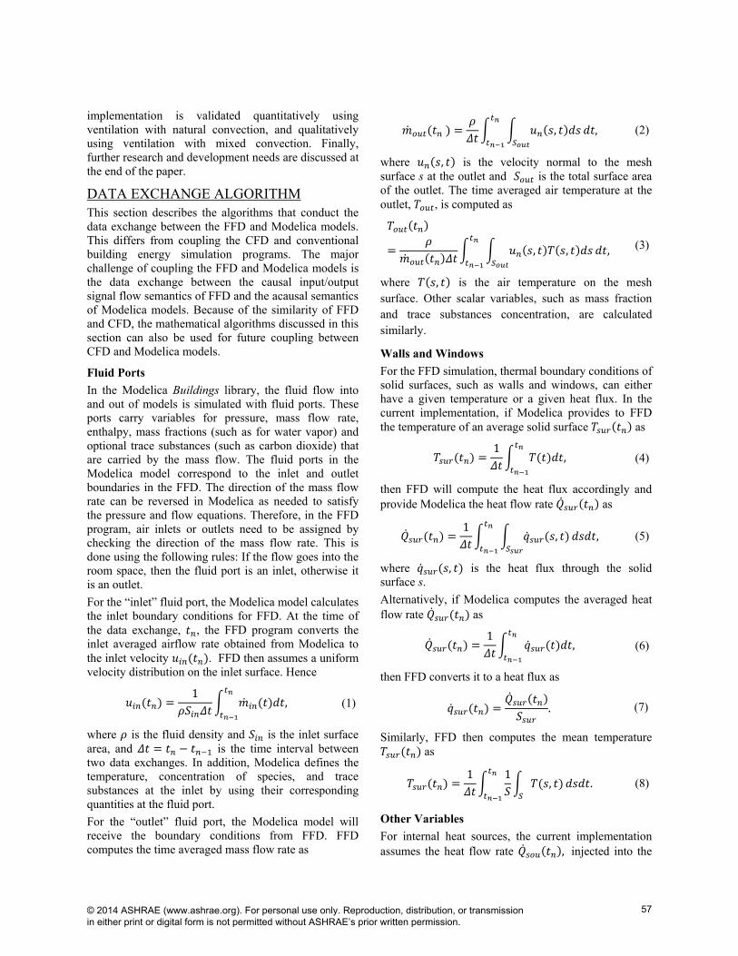
DATA SYNCHRONIZATION As shown in Figure 1, our implementation uses a data synchronization strategy between FFD and Modelica that is based on a zero-order hold of the respective input signals. At time step , corresponding data are exchanged. They are then kept constant in each individual program until the next synchronization step. Regardless of this, each program may use smaller time steps for its own integration between synchronization steps. This synchronization strategy is semantically equivalent to the one used by the Building Controls Virtual Test Bed (BCVTB) (Wetter, 2011). However, the BCVTB is a middleware used to facilitate the data exchange between two programs while we, on the other hand, applied direct data exchanges.

Figure 1 Data synchronization between the FFD and

Modelica models

IMPLEMENTATION The above algorithms have been implemented in the FFD program and the Modelica Buildings library. In the current implementation, Modelica is the master of the coupled simulation and FFD is the slave. Modelica defines the coupled simulation period and the next synchronization time. It also launches and terminates the FFD simulation. Since most of the implementation in the Modelica models can be used for coupled simulation with not only FFD but also CFD programs,

the term “CFD” is used in the related Modelica model names when it is applicable.

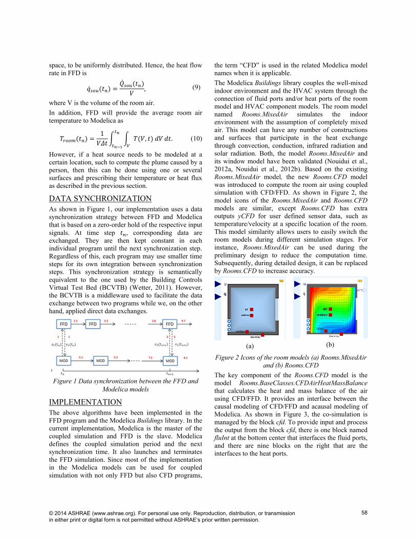
The Modelica Buildings library couples the well-mixed indoor environment and the HVAC system through the connection of fluid ports and/or heat ports of the room model and HVAC component models. The room model named Rooms.MixedAir simulates the indoor environment with the assumption of completely mixed air. This model can have any number of constructions and surfaces that participate in the heat exchange through convection, conduction, infrared radiation and solar radiation. Both, the model Rooms.MixedAir and its window model have been validated (Nouidui et al., 2012a, Nouidui et al., 2012b). Based on the existing Rooms.MixedAir model, the new Rooms.CFD model was introduced to compute the room air using coupled simulation with CFD/FFD. As shown in Figure 2, the model icons of the Rooms.MixedAir and Rooms.CFD models are similar, except Rooms.CFD has extra outputs yCFD for user defined sensor data, such as temperature/velocity at a specific location of the room. This model similarity allows users to easily switch the room models during different simulation stages. For instance, Rooms.MixedAir can be used during the preliminary design to reduce the computation time. Subsequently, during detailed design, it can be replaced by Rooms.CFD to increase accuracy.

(a)

(b)

Figure 2 Icons of the room models (a) Rooms.MixedAir and (b) Rooms.CFD

The key component of the Rooms.CFD model is the model Rooms.BaseClasses.CFDAirHeatMassBalance that calculates the heat and mass balance of the air using CFD/FFD. It provides an interface between the causal modeling of CFD/FFD and acausal modeling of Modelica. As shown in Figure 3, the co-simulation is managed by the block cfd. To provide input and process the output from the block cfd, there is one block named fluInt at the bottom center that interfaces the fluid ports, and there are nine blocks on the right that are the interfaces to the heat ports.


58

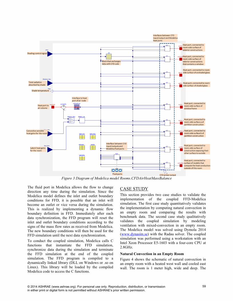
Figure 3 Diagram of Modelica model Rooms.CFDAirHeatMassBalance

The fluid port in Modelica allows the flow to change direction any time during the simulation. Since the Modelica model defines the inlet and outlet boundary conditions for FFD, it is possible that an inlet will become an outlet or vice versa during the simulation. This is realized by implementing a dynamic flow boundary definition in FFD. Immediately after each data synchronization, the FFD program will reset the inlet and outlet boundary conditions according to the signs of the mass flow rates as received from Modelica. The new boundary conditions will then be used for the FFD simulation until the next data synchronization.

To conduct the coupled simulation, Modelica calls C functions that instantiate the FFD simulation, synchronize data during the simulation and terminate the FFD simulation at the end of the coupled simulation. The FFD program is compiled to a dynamically linked library (DLL on Windows or .so on Linux). This library will be loaded by the compiled Modelica code to access the C functions.

CASE STUDY This section provides two case studies to validate the implementation of the coupled FFD-Modelica simulation. The first case study quantitatively validates the implementation by computing natural convection in an empty room and comparing the results with benchmark data. The second case study qualitatively validates the coupled simulation by modeling ventilation with mixed-convection in an empty room. The Modelica model was solved using Dymola 2014 (www.dynasim.se) with the Radau solver. The coupled simulation was performed using a workstation with an Intel Xeon Processor E5-1603 with a four-core CPU at 2.8GHz.

Natural Convection in an Empty Room

Figure 4 shows the schematic of natural convection in an empty room with a heated west wall and cooled east wall. The room is 1 meter high, wide and deep. The


59

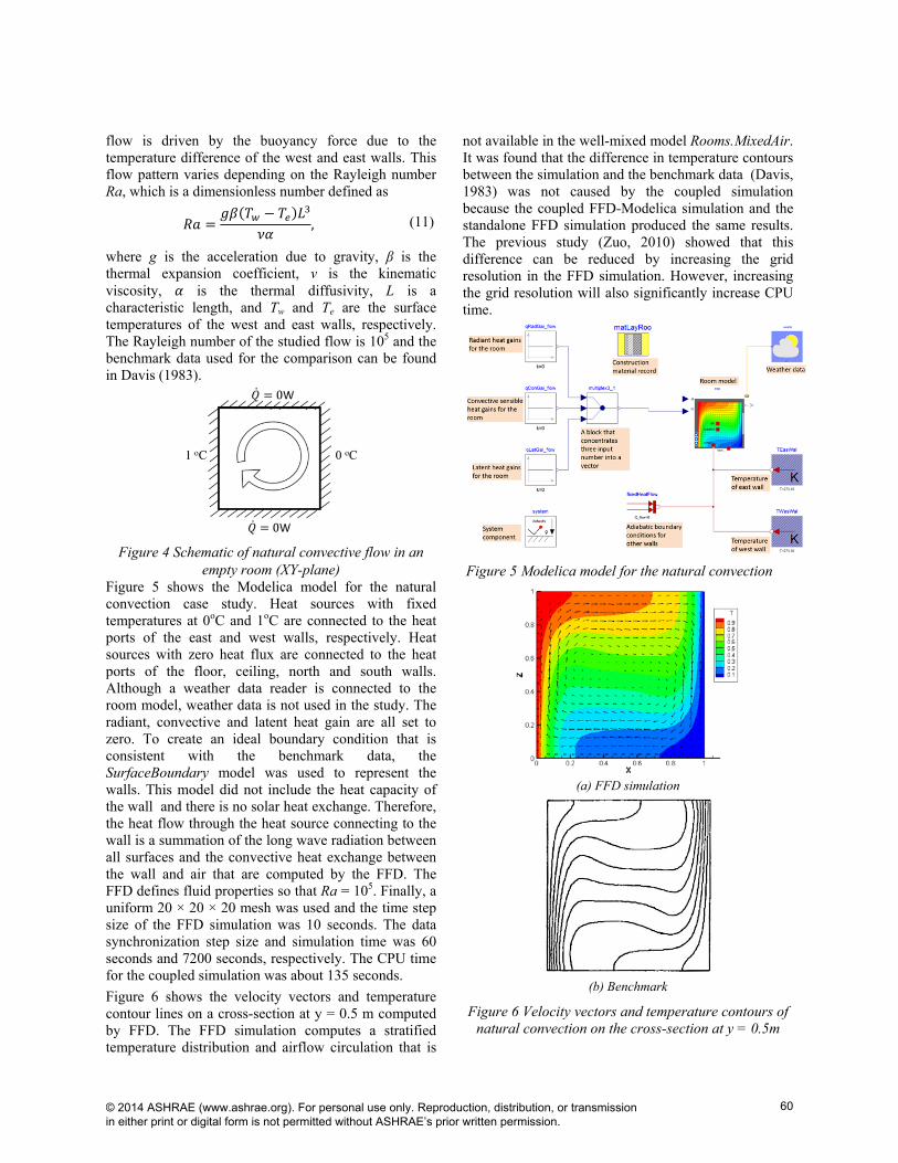
flow is driven by the buoyancy force due to the temperature difference of the west and east walls. This flow pattern varies depending on the Rayleigh number Ra, which is a dimensionless number defined as

, (11)

where g is the acceleration due to gravity, β is the thermal expansion coefficient, ν is the kinematic viscosity, is the thermal diffusivity, L is a characteristic length, and Tw and Te are the surface temperatures of the west and east walls, respectively. The Rayleigh number of the studied flow is 105 and the benchmark data used for the comparison can be found in Davis (1983).

Figure 4 Schematic of natural convective flow in an

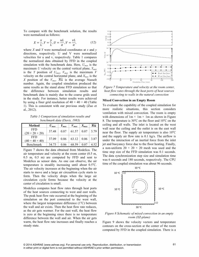
empty room (XY-plane) Figure 5 shows the Modelica model for the natural convection case study. Heat sources with fixed temperatures at 0oC and 1oC are connected to the heat ports of the east and west walls, respectively. Heat sources with zero heat flux are connected to the heat ports of the floor, ceiling, north and south walls. Although a weather data reader is connected to the room model, weather data is not used in the study. The radiant, convective and latent heat gain are all set to zero. To create an ideal boundary condition that is consistent with the benchmark data, the SurfaceBoundary model was used to represent the walls. This model did not include the heat capacity of the wall and there is no solar heat exchange. Therefore, the heat flow through the heat source connecting to the wall is a summation of the long wave radiation between all surfaces and the convective heat exchange between the wall and air that are computed by the FFD. The FFD defines fluid properties so that Ra = 105. Finally, a uniform 20 × 20 × 20 mesh was used and the time step size of the FFD simulation was 10 seconds. The data synchronization step size and simulation time was 60 seconds and 7200 seconds, respectively. The CPU time for the coupled simulation was about 135 seconds.

Figure 6 shows the velocity vectors and temperature contour lines on a cross-section at y = 0.5 m computed by FFD. The FFD simulation computes a stratified temperature distribution and airflow circulation that is

not available in the well-mixed model Rooms.MixedAir. It was found that the difference in temperature contours between the simulation and the benchmark data (Davis, 1983) was not caused by the coupled simulation because the coupled FFD-Modelica simulation and the standalone FFD simulation produced the same results. The previous study (Zuo, 2010) showed that this difference can be reduced by increasing the grid resolution in the FFD simulation. However, increasing the grid resolution will also significantly increase CPU time.

Figure 5 Modelica model for the natural convection

(a) FFD simulation

(b) Benchmark

Figure 6 Velocity vectors and temperature contours of natural convection on the cross-section at y = 0.5m


60

To compare with the benchmark solution, the results were normalized as follows:

, , , , (12)

where X and Y were normalized coordinates at x and y directions, respectively. U and V were normalized velocities for u and v, respectively. Table 1 compares the normalized data obtained by FFD in the coupled simulation with the benchmark data. Here, Umax is the maximum U velocity on the central vertical plane, Ymax is the Y position of Umax, Vmax is the maximum V velocity on the central horizontal plane, and Xmax is the X position of the Vmax. is the average Nusselt number. Again, the coupled simulation produced the same results as the stand alone FFD simulation so that the difference between simulation results and benchmark data is mainly due to the coarse grids used in the study. For instance, better results were achieved by using a finer grid resolution of 40 × 40 × 40 (Table 1). This is consistent with our previous study (Zuo et al., 2012).

Table 1 Comparison of simulation results and benchmark data (Davis, 1983)

Method Umax Ymax Vmax Xmax FFD

(20 × 20 × 20) 37.48 0.87 61.57 0.07 3.79

FFD (40 × 40 × 40)

37.09 0.86 63.12 0.06 3.87

Benchmark 34.73 0.86 68.59 0.07 4.52

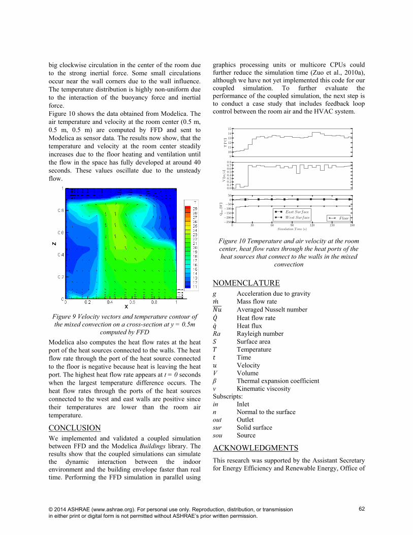
Figure 7 shows the data obtained from Modelica. The air temperature and velocity at the room center (0.5 m, 0.5 m, 0.5 m) are computed by FFD and sent to Modelica as sensor data. As one can observe, the air temperature is steadily increasing until about 0.5oC. The air velocity increases at the beginning when the air starts to move and a large air circualtion cycle starts to form. Then the velocity drops when the large air circulation cycle forms because the velocity at the center of circulation is small.

Modelica computes heat flow rates through heat ports of the heat sources connecting to west and east walls. The peak heat flow rate occurred at the beginning of the simulation on the port connected to the west wall, where the largest temperature difference (1oC) between the wall and air exists. Then the heat flow rate reduces, as the air gets warmer. For the east wall, the heat flow is zero at the beginning since there is no temperature difference between the wall and air. When the air gets warm, the heat flow rate increases and finally reaches a steady state.

Figure 7 Temperature and velocity at the room center, heat flow rates through the heat ports of heat sources

connecting to walls in the natural convection

Mixed Convection in an Empty Room

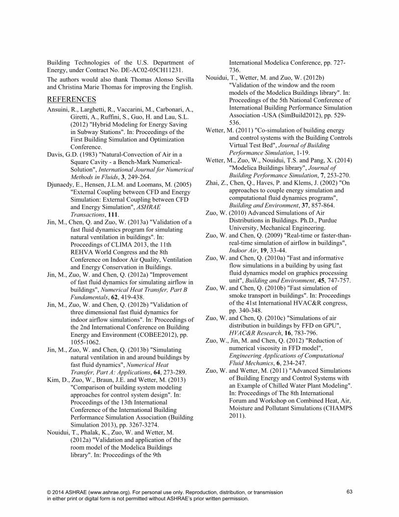
To evaluate the capability of the coupled simulation for more realistic situations, this section considers ventilation with mixed convection. The room is empty with dimensions of 1m × 1m × 1m as shown in Figure 8. The temperature is 30oC on the floor and 10oC on the ceiling and all walls. The inlet is located on the west wall near the ceiling and the outlet is on the east wall near the floor. The supply air temperature is also 10oC and the supply air flow rate is 0.1 kg/s. The airflow is under the interaction of an inertial force from the inlet jet and buoyancy force due to the floor heating. Finally, a non-uniform 20 × 20 × 20 mesh was used and the time step size of the FFD simulation was 0.1 seconds. The data synchronization step size and simulation time was 6 seconds and 180 seconds, respectively. The CPU time of the coupled simulation was about 96 seconds.

Figure 8 Schematic of mixed convection in an empty room (XZ-plane)

Figure 9 shows the velocity vectors and temperature contours on the cross-section at the center of the room computed by FFD in the coupled simulation. There is a

0.0

0.1

0.2

0.3

0.4

0.5

T[◦C]

10−5

10−4

10−3

V[m

/s]

0 20 40 60 80 100 120Simulation T ime (min)

−0.6

−0.4

−0.2

0.0

0.2

Qsu

r[W

]

East Surface

West Surface


61

big clockwise circulation in the center of the room due to the strong inertial force. Some small circulations occur near the wall corners due to the wall influence. The temperature distribution is highly non-uniform due to the interaction of the buoyancy force and inertial force. Figure 10 shows the data obtained from Modelica. The air temperature and velocity at the room center (0.5 m, 0.5 m, 0.5 m) are computed by FFD and sent to Modelica as sensor data. The results now show, that the temperature and velocity at the room center steadily increases due to the floor heating and ventilation until the flow in the space has fully developed at around 40 seconds. These values oscillate due to the unsteady flow.

Figure 9 Velocity vectors and temperature contour of the mixed convection on a cross-section at y = 0.5m

computed by FFD

Modelica also computes the heat flow rates at the heat port of the heat sources connected to the walls. The heat flow rate through the port of the heat source connected to the floor is negative because heat is leaving the heat port. The highest heat flow rate appears at t = 0 seconds when the largest temperature difference occurs. The heat flow rates through the ports of the heat sources connected to the west and east walls are positive since their temperatures are lower than the room air temperature.

CONCLUSION We implemented and validated a coupled simulation between FFD and the Modelica Buildings library. The results show that the coupled simulations can simulate the dynamic interaction between the indoor environment and the building envelope faster than real time. Performing the FFD simulation in parallel using

graphics processing units or multicore CPUs could further reduce the simulation time (Zuo et al., 2010a), although we have not yet implemented this code for our coupled simulation. To further evaluate the performance of the coupled simulation, the next step is to conduct a case study that includes feedback loop control between the room air and the HVAC system.

Figure 10 Temperature and air velocity at the room center, heat flow rates through the heat ports of the heat sources that connect to the walls in the mixed

convection

NOMENCLATURE g Acceleration due to gravity

Mass flow rate Averaged Nusselt number

Heat flow rate Heat flux

Ra Rayleigh number Surface area Temperature Time Velocity

V Volume β Thermal expansion coefficient ν Kinematic viscosity Subscripts: in Inlet n Normal to the surface out Outlet sur Solid surface sou Source

ACKNOWLEDGMENTS

This research was supported by the Assistant Secretary for Energy Efficiency and Renewable Energy, Office of

9

10

11

12

13

14

15

T[◦C]

0.00.10.20.30.40.50.60.70.8

V[m

/s]

0 30 60 90 120 150 180Simulation T ime (s)

−250

−200

−150

−100

−50

0

50

Qsur[W

]Floor

East Surface

West Surface


62

Building Technologies of the U.S. Department of Energy, under Contract No. DE-AC02-05CH11231.

The authors would also thank Thomas Alonso Sevilla and Christina Marie Thomas for improving the English.

REFERENCES Ansuini, R., Larghetti, R., Vaccarini, M., Carbonari, A.,

Giretti, A., Ruffini, S., Guo, H. and Lau, S.L. (2012) "Hybrid Modeling for Energy Saving in Subway Stations". In: Proceedings of the First Building Simulation and Optimization Conference.

Davis, G.D. (1983) "Natural-Convection of Air in a Square Cavity - a Bench-Mark Numerical-Solution", International Journal for Numerical Methods in Fluids, 3, 249-264.

Djunaedy, E., Hensen, J.L.M. and Loomans, M. (2005) "External Coupling between CFD and Energy Simulation: External Coupling between CFD and Energy Simulation", ASHRAE Transactions, 111.

Jin, M., Chen, Q. and Zuo, W. (2013a) "Validation of a fast fluid dynamics program for simulating natural ventilation in buildings". In: Proceedings of CLIMA 2013, the 11th REHVA World Congress and the 8th Conference on Indoor Air Quality, Ventilation and Energy Conservation in Buildings.

Jin, M., Zuo, W. and Chen, Q. (2012a) "Improvement of fast fluid dynamics for simulating airflow in buildings", Numerical Heat Transfer, Part B Fundamentals, 62, 419-438.

Jin, M., Zuo, W. and Chen, Q. (2012b) "Validation of three dimensional fast fluid dynamics for indoor airflow simulations". In: Proceedings of the 2nd International Conference on Building Energy and Environment (COBEE2012), pp. 1055-1062.

Jin, M., Zuo, W. and Chen, Q. (2013b) "Simulating natural ventilation in and around buildings by fast fluid dynamics", Numerical Heat Transfer, Part A: Applications, 64, 273-289.

Kim, D., Zuo, W., Braun, J.E. and Wetter, M. (2013) "Comparison of building system modeling approaches for control system design". In: Proceedings of the 13th International Conference of the International Building Performance Simulation Association (Building Simulation 2013), pp. 3267-3274.

Nouidui, T., Phalak, K., Zuo, W. and Wetter, M. (2012a) "Validation and application of the room model of the Modelica Buildings library". In: Proceedings of the 9th

International Modelica Conference, pp. 727-736.

Nouidui, T., Wetter, M. and Zuo, W. (2012b) "Validation of the window and the room models of the Modelica Buildings library". In: Proceedings of the 5th National Conference of International Building Performance Simulation Association -USA (SimBuild2012), pp. 529-536.

Wetter, M. (2011) "Co-simulation of building energy and control systems with the Building Controls Virtual Test Bed", Journal of Building Performance Simulation, 1-19.

Wetter, M., Zuo, W., Nouidui, T.S. and Pang, X. (2014) "Modelica Buildings library", Journal of Building Performance Simulation, 7, 253-270.

Zhai, Z., Chen, Q., Haves, P. and Klems, J. (2002) "On approaches to couple energy simulation and computational fluid dynamics programs", Building and Environment, 37, 857-864.

Zuo, W. (2010) Advanced Simulations of Air Distributions in Buildings. Ph.D., Purdue University, Mechanical Engineering.

Zuo, W. and Chen, Q. (2009) "Real-time or faster-than-real-time simulation of airflow in buildings", Indoor Air, 19, 33-44.

Zuo, W. and Chen, Q. (2010a) "Fast and informative flow simulations in a building by using fast fluid dynamics model on graphics processing unit", Building and Environment, 45, 747-757.

Zuo, W. and Chen, Q. (2010b) "Fast simulation of smoke transport in buildings". In: Proceedings of the 41st International HVAC&R congress, pp. 340-348.

Zuo, W. and Chen, Q. (2010c) "Simulations of air distribution in buildings by FFD on GPU", HVAC&R Research, 16, 783-796.

Zuo, W., Jin, M. and Chen, Q. (2012) "Reduction of numerical viscosity in FFD model", Engineering Applications of Computational Fluid Mechanics, 6, 234-247.

Zuo, W. and Wetter, M. (2011) "Advanced Simulations of Building Energy and Control Systems with an Example of Chilled Water Plant Modeling". In: Proceedings of The 8th International Forum and Workshop on Combined Heat, Air, Moisture and Pollutant Simulations (CHAMPS 2011).


63

coupled simulation of indoor environment, hvac...

Documents