coupled geomechanical and reactive geochemical … · coupled geomechanical and reactive...
TRANSCRIPT

PROCEEDINGS, Thirty-Eighth Workshop on Geothermal Reservoir Engineering
Stanford University, Stanford, California, February 11-13, 2013
SGP-TR-198
COUPLED GEOMECHANICAL AND REACTIVE GEOCHEMICAL SIMULATIONS FOR
FLUID AND HEAT FLOW IN ENHANCED GEOTHERMAL RESERVOIRS
Yi Xiong, Litang Hu and Yu-Shu Wu
Department of Petroleum Engineering
Colorado School of Mines
1500 Illinois Street,
Golden, CO, 80401, USA
e-mail: [email protected]
ABSTRACT
A major concern in development of fractured
reservoirs in Enhanced Geothermal Systems (EGS) is
to achieve and maintain adequate injectivity, while
avoiding short-circuiting flow paths. The injection
performance and flow paths are dominated by
fracture rock permeability. The evolution of fracture
permeability can be made by change in temperature
or pressure induced rock deformation and
geochemical reaction. Especially in fractured media,
the change of fracture apertures due to
geomechanical deformation and mineral
precipitation/dissolution could have a major impact
on reservoir long-term performance. A coupled
thermal-hydrological-mechanical-chemical (THMC)
model is in general necessary to examine the
reservoir behavior in EGS.
This paper presents a numerical model, TOUGH2-
EGS, for simulating coupled THMC processes in
enhanced geothermal reservoirs. This simulator is
built by coupling mean stress calculation and reactive
geochemistry into the existing framework of
TOUGH2 (Pruess et al., 1999), a well-established
numerical simulator for geothermal reservoir
simulation. The geomechanical model is fully-
coupled as mean stress equations, which are solved
simultaneously with fluid and heat flow equations.
The flow velocity and phase saturations are used for
reactive geochemical transport simulation after
solution of the flow and heat equations in order to
sequentially couple reactive geochemistry at each
time step. The fractured medium is represented by
multi interacting continua (MINC) model in the
simulations.
We perform coupled THMC simulations to examine
a prototypical EGS reservoir for fracture aperture
change at the vicinity of the injection well. The
results demonstrate the strong influence of
temperature-induced rock deformation effects in the
short-term and intermediate- and long-term influence
of chemical effects. It is observed that the fracture
enhancement by thermal-mechanical effect can be
counteracted by the precipitation of minerals, initially
dissolved into the low temperature injected water.
We conclude that the temperature and chemical
composition of injected water can be modified to
improve reservoir performance by maintaining or
even enhancing fracture network under both
geomechanical and reactive geochemical effects.
INTRODUCTION
The successful development of enhanced geothermal
systems (EGS) highly depends on the reservoir
fracture network of hot dry rock (HDR) and its
hydraulic properties. The geomechanical processes
under subsurface reservoir condition are prevalent in
the EGS applications. For example, Tsang and Chin-
Fu (1999) presented that hydraulic properties of
fracture rocks are subjected to change under reservoir
mechanical effects. Rutqvist et al. (2002) investigated
the stress-induced changes in the fracture porosity,
permeability and capillary pressure. It is also well
known that the cold water injection and steam or hot
water extraction have thermo-poro-elastic effects for
EGS reservoirs.
On the other hand, the strong impacts of geochemical
reaction on the EGS reservoirs have been observed in
the commercial EGS fields in the past few years.
Kiryukhin et al.(2004) modeled the reactive chemical
process based on the field data from tens of
geothermal fields in Kamchatka (Russia) and Japan.
In addition, Xu et al. (2004a) presented the reactive
transport model of injection well scaling and
acidizing at Tiwi field in Philippines. Montalvo et al.
(2005) studied the calcite and silica scaling problems
with exploratory model for Ahuachapan and Berlin
geothermal fields in El Salvador. The typical
chemical reactions between fluids and rock minerals

in EGS reservoirs, the mineral dissolution and
precipitation, should be fully evaluated and predicted
in order to assist the development of geothermal
energy.
The numerical simulation is a powerful tool to model
the geomechanical and geochemical processes for
EGS reservoirs. The research efforts have been put in
this direction and a few EGS reservoir simulation
tools are developed. For example, Rutqvist et al.
(2002) linked TOUGH2 (Pruess et al., 1999) and
FLAC3D for modeling of THM process. Wang and
Ghassemi (2012) presented a 3D thermal-poroelastic
model for geothermal reservoir simulation.
Fakcharoenphol and Wu (2012) developed the fully
implicit flow and geomechanics model for EGS
reservoirs. The coupled THC simulator,
TOUGHREACT (Xu et al., 2004b), has the
capability to model the multi-components multi-
phase fluid flow, solute transport and chemical
reactions in the subsurface systems. However, the
single programs coupling THMC processes are rarely
available. Taron et al. (2009) introduced one
“modular” approach to generate a coupled THMC
simulator by coupling the capabilities of
TOUGHREACT with the mechanical framework of
FLAC3D. Compared with single coupled program,
although the modular approach may be more rapid
and less expensive, it may result in the issues of
flexibility and accuracy.
In this paper, we present one single coupled THMC
simulator for geothermal reservoir modeling,
TOUGH2-EGS. This simulator is built by coupling
mean stress calculation and geochemical reactions
into the existing framework of TOUGH2 (Pruess et
al., 1999), a well-established numerical simulator for
subsurface thermal-hydrological analysis with multi-
phase, multi-component fluid and heat flow. The
mechanical model is fully-coupled as the mean stress
equations, solved simultaneously with fluid and heat
flow equations. In order to sequentially couple the
chemical process, the solution of fluid and heat flow
equations provides the flow velocity and phase
saturation to compute the solute transport and
chemical reactions at each time step.
This paper is organized as follows. First, we present
the mathematical model for coupling geomechanical
and geochemical processes. Then the simulation
procedure for coupling THMC processes is
introduced. Finally, one application example for
simulating the THMC processes at the vicinity of the
injection well is presented. In this application
example, we analyze the fracture aperture evolution
due to the mechanical and chemical effects through
three cases. By comparing the base case and modified
cases, it is found that the mechanical and chemical
process may be in favor of or undermine the fracture
network by modifying chemical components and
temperature of the injection water.
MATHEMATICAL MODEL
Formulation of Fluid and Heat Flow
The fluid and heat flow equations are formulated
based on mass and energy conservation. Following
the integral formats of TOUGH2, the general mass
and energy balance equation can be written as
ˆ
n n n
k k k
n n n
V V
dM dV F nd q dV
dt
(1)
The integration is over an arbitrary subdomain or
representative element volume (REV) Vn of EGS
reservoir flow system, which is bounded by the
closed surface Гn. The quantity M in the
accumulation term represents mass or energy per
volume, with k=1, 2 labeling the component of water
and air in the EGS reservoir and k=3 labeling heat
“component” for energy balance. F donates the mass
or heat flux, and q donates sinks and sources. n is the
normal vector on the surface element dГn, pointing
inward into Vn. The general form of mass
accumulation for component k is
k kM S X
(2)
The total mass of component k is obtained by
summing over the fluid phase β (= liquid or gas). 𝜙 is
the porosity, Sβ is the saturation of phase β, ρβ is the
density of phase β, and Xβk is the mass fraction of
component k present in phase β. Similarly the heat
accumulation is
3 1k
R RM C T S u
(3)
where ρR and CR is the grain density and specific heat
of the rock. T is the temperature and uβ is the specific
internal energy in phase β.
The mass flux includes advective and diffusive flux
(hydrodynamic dispersion and molecular diffusion)
as
k k k
adv disF F F (4)
Advective flux is the sum over phases,
k k
advF X F
(5)

The advective flux of phase β is given by the
multiphase Darcy’s law as
rkF v k P g
(6)
where vβ is Darcy velocity of phase β, k is the
absolute permeability; krβ and µβ are relative
permeability and viscosity of phase β respectively. Pβ
is the fluid pressure of the phase, which is given by
the pressure of reference phase and the capillary
pressure between the phases.
In addition to the advective flow, the mass transport
also occurs through hydrodynamic dispersion and
molecular diffusion defined as follows.
k k k
dispF D X
(7)
0
k k k
diffF d X (8)
k k k
dis disp diffF F F (9)
where Dβk is the hydrodynamic dispersion tensor; dβ
k
is the molecular diffusion coefficient for component k
in phase β. τ0 and τβ are the tortuosity factors,
respectively depending on rock property and phase
saturation.
The heat flow is governed by conduction and
convection.
3kF T h F
(10)
where λ is thermal conductivity, and hβ is specific
enthalpy in phase β. Fβ is given by equation (6).
Formulation of Geomechanics
The fully coupled mechanical model assumes that
each grid block can move as an elastic material and
obey the generalized Hooke’s law.
Under the assumption of linear elastic with small
strain for thermo-poro-elastic system, the stress
equilibrium can be expressed as follows (Jaeger et
al., 2007, Winterfeld and Wu, 2011)
3
2 , , ,
kk ref xx yy zz
kk
P K T T
G k x y z
(11)
where σ is the normal stress, α is the Biot’s
coefficient, β is the linear thermal expansion
coefficient, K is the bulk modulus, λ is the Lame’s
constant, G is the shear modulus and ε is the strain.
The subscript k stands for the directions.
Summing over the x, y and z component of equation
(11) gives the trace of Hooke’s law for poroelastic
medium.
33
2
3
xx yy zz
ref
xx yy zz
P K T T
G
(12)
Rewrite equation (12) in terms of mean normal stress
and volumetric strain as
23
3m ref vP K T T G
(13)
where σm and εv are the mean normal stress and
volumetric strain.
The poroelastic version of the Navier equations may
be written as
2
3
0
P K T G u
G u F
(14)
where u is the displacement vector and F is the
body force. The divergence of the displacement
vector is the volumetric strain as
yx zxx yy zz v
uu uu
x y z
(15)
Take partial derivatives with respect to x for the x-
component of equation (14), with respect to y for the
y-component and with respect to z for the z-
component, and add together to achieve the following
equation.
2 2 23 2 0P K T G u F (16)
Solving εv in equation (13) and substitute u in
equation (16) gives us the governing equation
coupling pore pressure, temperature and mean normal
stress.
2 2 23 1 2 1 23
1 1m F P K T
(17)
where υ is the Poisson’s ratio, substituting the λ and
G of the original equations with the appropriate
relationships.
The multiple interacting continua (MINC) approach
(Pruess and Narasimhan, 1985) is used to simulate
facture and matrix flow and interactions in our
model. From the dual porosity poroelastic Navier
equations (Bai and Roegiers, 1994) with the similar
steps as before, the governing geomechanical
equation for each set of MINC blocks can be derived
as
2 2 2
1
3 1 2 1 23
1 1
N
m i i i ii
F P K T
(18)
where N is the total number of MINC blocks for each
set.
Formulation of Reactive Chemistry
Due to the complexity of multiphase fluid and heat
flow, fluid-rock interaction and the strong non-
linearity in mass and energy conservation equation
for geochemical process, it is costly to develop the
fully coupled chemical reaction model (Zhang et al.,
2012). We therefore take the approach same as the
TOUGHREACT to sequentially couple the chemical
reaction process, which iteratively solves solute
transport and chemical reactions.
Solute transport
The solute transport occurring in the liquid phase also
follows the general mass balance equation (1), where
accumulation and flux terms may be expressed
k
k klM S C (19)
1...k
l kl l l kl lF v C S D C k N (20)
where Nl is the total number of the chemical
components (species) in the liquid phase; Ckl is the
concentration of the kth
species in liquid phase; vl is
the Darcy velocity, Dl is the diffusion coefficient.
It is convenient to select a subset of aqueous species
as basis species (primary species) for representing a
geochemical system. All other species, including
aqueous complexes, precipitated species, are called
secondary species. The number of secondary species
must be equal to the number of independent
reactions. Any of the secondary species can be
represented as a linear combination of basis species
as
1
1...cN
i ij j Rj
C v C i N
(21)
where Nc is the number of the primary species and NR
is the number of the secondary species, j is the
primary species index and i is the secondary species
index, vij is the stoichiometric coefficient of jth
primary species in the ith
reaction. Likewise, the
concentration of aqueous complex can be expressed
as function of that of primary species
1 1
1
c
ij ij
Nv v
i i i j j
j
c K c
(22)
where ci is the concentration of the ith
aqueous
complex, and cj is the concentration of the jth
primary
species, γ is the thermodynamic activity coefficients
and Ki is the equilibrium constant. Therefore it is
sufficient to only solve primary species concentration
in the transport solute; the secondary species and
aqueous complex can be readily represented.
Mineral dissolution/precipitation
The mineral saturation ratio can be expressed as
1 1 1
1
1...c
mj
Nv mj
m m m m j j p
j
X K c m N
(23)
where Np is the number of minerals at equilibrium
conditions, m is he equilibrium mineral index, Ωm is
mineral saturation ratio, Xm is the mole fraction of
the mth
mineral phase, λm is its thermodynamic
activity coefficient (Xm and λm are taken to one for
pure mineral phases), and Km is the corresponding
equilibrium constant. At equilibrium condition
0m mSI Log (24)
where SIm is the mineral saturation index.
For the kinetic mineral dissolution/precipitation, the
kinetic rate could be functions of non-primary
species. We usually consider the species appearing in
rate laws as the primary species. In our model, we
use the rate expression given by Lasaga et al. (1994),
1, 2,..., 1 1...n Nc n n n qr f c c c k A n N (25)
where Nq is the number of minerals at kinetic
conditions, the positive values of rn indicate
dissolution and negative values for precipitation, kn is
the rate constant (moles per unit mineral surface area
and unit time) which depends on the temperature, An
is the specific reactive surface area per kg H2O. Ωn is
the kinetic mineral saturation ratio defined as
equation (23). The parameters θ and η, can be
determined from experiment, usually assumed to be
unity. The reaction rate constant kn is dependent on
temperature and usually rate constants are reported at
25oC. For a reasonable approximation, the rate
constant could be handled via the Arrhenius equation
(Lasaga 1984; Steefel and Lasaga 1994),
25
1 1exp
298.15aE
k kR T
(26)

where Ea is the activation energy, k25 is the rate
constant at 25oC, R is gas constant, T is absolute
temperature.
Numerical Model
The general mass and energy balance equation (1) is
discretized in space using integral finite difference
method (IFD; Narasimhan and Witherspoon, 1976).
By introducing proper average volume and
approximating surface integrals to a discrete sum of
averages over surface segments, the equation (1) has
the residual form as equation (27) with time and
space discretization.
, 1 , 1 , , 1 , 1 0k t k t k t k t k t
n n n nm nm n nmn
tR M M A F V q
V
(27)
where R is the residual of component k ( k = 1 and 2
stands for components of water and air, and 3 stands
for the heat) for grid block n, t+1 donates the current
time level, m donates the neighboring grid blocks of
n, Anm and Fnm are the interface area and flux between
them.
In order to fully couple the geomechanical effect, the
mean stress governing equation (17) needs to be
discretized to the same form as equation (27).
Applying the divergence theorem and approximating
surface integrals to a discrete sum over surface
segments, the mean stress equation has the following
discretized residual form,
4, 1 3 1 2 1 23 0
1 1
t
n mnm
R F P K T A
(28)
where m is the neighboring grid blocks of n and Anm
is the interface area between them. There are total
four residual equations with four primary variable,
pressure, temperature, air mass fraction and mean
normal stress, which are solved simultaneously
through Newton-Raphson methods. After solving the
THM process, the Darcy velocity and phase
saturation are used to compute solute transport and
chemical reaction, which also follows a similar
numerical method.
RESERVOIR EVOLUTION UNDER THMC
EFFECTS
The EGS reservoir properties, such as permeability,
porosity, block volume, and capillaries etc., are
subject to changes under the geomechanical and
geochemical effects, and those changes may feedback
to the heat and fluid flows. The relationship between
effective stress σ’ and permeability k, porosity ϕ has
been investigated through many research efforts
(Ostensen et al., 1986; McKee et al., 1988; Davies
and Davies, 2001; Rutqvist et al., 2002).
' 'k k (29)
Our mechanical model implements those correlations
and the user can choose the proper one according to
the specific reservoir conditions.
The geochemical model considers the porosity
change due to mineral dissolution/precipitation as
follows.
1
1Nm
m u
cm
fr fr
(30)
where Nm is the number of reactive minerals and frm
is the mineral fraction in the containing rock
(Vmineral/Vmedium), fru is the non-reactive fraction. Since
frm of each mineral change, the porosity is updated at
each time step.
The above analysis applies to the independent THM
or THC processes. As for the THMC process, we
combine the fracture aperture change due to both
mechanical and chemical processes. The aperture
under the effective stress σ’ may be defined
empirically as (Rutqvist et al., 2002)
max exp ' exp 'm i m i ib b b b b d d (31)
where bm is the aperture under mechanical effect, bi is
the initial aperture under no stress, bmax is maximum
“mechanical” aperture and d is the constant defining
the non-linear stiffness of the fracture, σ’ and σi’ are
the current stress and initial stress. On the other hand,
chemical dissolution and precipitation could lead to
the change in fracture aperture Δbc under chemical
effect (Xu et al., 2004b).
0
0
c cc g
c
b b
(32)
0
f
g
f
bA
(33)
where bg is the initial aperture available for
precipitation (geometry aperture), which can be
calculate from the ratio of the initial fracture porosity
ϕ f0 to the fracture surface area Af. The total aperture
under THMC effects therefore is
1 1 1t t t t
m cb b b b (34)
where the t+1 and t means current and previous time
step; subscripts m and c means the mechanical and
chemical effects respectively. The changed fracture

aperture leads to the updated permeability, porosity
and capillary pressure. The possible relationships
between them are
31
1
12
t
tb
kW
(35)
1 1 1
1 1 2 30 0 0 0
1 2 3
t t tt b b b
b b b
(36)
0
0
0c c
kp p
k
(37)
where equation (35) is the cubic law (Snow, 1969;
Witherspoon et al., 1979) and W is the fracture space;
Rutqvist et al. (2002) derived equation (36) with
cubic-block conceptual model, and used J-function to
correct capillary pressure as equation (37). The
superscripts t+1 is the current time step and 0 is the
initial time.
SIMULATION LOGIC AND PROCEDURE
Our EGS reservoir simulator is a single program built
on the framework of TOUGH2, fully coupling
geomechanics and sequentially coupling reactive
geochemistry. The figure 1 describes the program
process. It mainly includes two modules, the
geomechanical and geochemical modules. Although
the figure shows the THMC process, the two modules
could be run independently only for THM or THC
according to the selection in the input files.
The THMC coupling logic is as follows: The input
files, including rock hydrologic and geomechanical
properties, computing parameters, solute and
chemical parameters, etc. are read into the program.
Before stepping into the main cycle, the program
initializes the stress state and chemical state variables
at initial condition. For each time step, the THM
variables are firstly solved and the results, such as
fluid velocity, phase saturations and temperature
distributions, will be used to solve solute transport
and chemical reactions. The solute transport and
chemical reactions are solved iteratively until
chemical state converges. The time control cycle
repeats until the target time is reached.
APPLICATION AND DISCUSSION
In the application example, we present one
prototypical EGS reservoir to simulate THMC
process of the vicinity of the injection well. As
shown in the figure 2, the fractured reservoir is
overlain by the caprock and the injection well is in
the middle of the simulated area. The mesh is
generated with radial and vertical (R-Z) dimensions
and logarithmic distribution in radial direction to
capture the subtle effects around the wellbore. The
tables 1 and 2 list the reservoir mechanical and
chemical properties.
Read input files
Time step +1
More time
stepsNo
Initialzie transport and chemical
variables
Stop
Initialize fluid, heat and stress
variables
Yes
Build Jacobian matrix for residual
equations
of water,air, heat and stress
Solve solute transport of
chemical components
Call chemical reaction model
Chemical state
converged
No
ConvergedCall linear solver and update
variables
Update secondary and
primary variables
(P,T, air mass fraction, stress)
Update chemical variables
No
Yes
Input Darcy velocity, etc.
Input concentration values
Yes
Figure 1: Simulation process for THMC coupling
R 1000m
….. …..
Figure 2: Geometry of the simulated area and initial
temperature, pressure and mean stress
THM Module
Chemical Module
Caprock
Fractured
Reservoir T = 260ºC
P = 12.6 MPa σ = 42.0 MPa
Injection Rate = 38 kg/s

Table 1: Reservoir and material properties
Properties Values
Young’s Modulus (GPa) 14.4
Poisson’s ratio (dimensionless) 0.20
Permeability (m2) 2.37×10⁻¹³
Porosity (dimensionless) 0.1
Pore compressibility(Pa-1) 5×10⁻¹⁰
Thermal expansion coefficient (ºC-1) 4.14×10⁻⁶
Rock grain specific heat (J/kg ºC) 1000
Rock grain density (kg/m3) 2750
Formation thermal conductivity (W/m ºC) 2.4
Constant d in Eq. (31) (Pa-1) 1.06×10⁻⁷
Maximum aperture in Eq. (31) (m) 1.86×10⁻⁴
Geometry aperture in Eq. (32) (m) 1.55×10⁻³
Biot’s coefficient (dimensionless) 1.0
Table 2: The chemical components for reservoir
initial water and injection water
Chemical
Species
Initial Water
Concentration
(mol/l)
Injection Water
Concentration
(mol/l)
Ca2+ 3.32×10⁻³ 1.0327×10⁻³
Mg2+ 8.62×10⁻⁶ 1.6609×10⁻⁶
Na+ 1.285×10⁻¹ 1.2734×10⁻¹
Cl- 1.418×10⁻¹ 1.418×10⁻¹
SiO2(aq) 1.218×10⁻² 1.1734×10⁻²
HCO3- 1.0423×10⁻³ 1.0423×10⁻³
SO42- 2.6272×10⁻⁴ 2.6272×10⁻⁴
K+ 1.5852×10⁻² 1.5852×10⁻²
AlO2- 0.059×10⁻⁴ 0.0205×10⁻⁴
The figure 3 shows the initial mineral composition of
reservoir rock by volume fractions. The volume
fraction of the mineral is the mineral volume divided
by total volume of solids, excluding the liquid
volume. The sum of the mineral volume fraction is
not necessary to be 1 because the remaining solid
fraction is considered to be un-reactive throughout
the whole process.
Figure 3: Initial mineral volume fraction
In order to represent a prototypical EGS reservoir, the
geomechanical and geochemical data are taken from
reasonable assumptions and from the Tiwi EGS field
of Philippines (Xu et al., 2004a; Takeno et al., 2000).
We run three simulation cases within one year to
investigate the THMC effects with changed chemical
composition and temperature of the injection water.
The base case has the injection temperature of 150 ºC
and chemical concentrations as table 2. The case 1
has the same injection temperature but lower
concentration of aqueous SiO2 in the injection water.
The case 2 has the same chemical concentration as
table 2 but with lower injection temperature of
120ºC.
Base Case
Figure 4: Reservoir effective mean stress evolution
Figure 5: Mineral volume fraction evolution
Figures 4 and 5 show the evolution of geomechanical
and geochemical states extending to 200m from the
injection well simulated in one year. The mechanical
and chemical effects on the reservoir are spatially and
temporally different. Spatially, the mechanical effect
has larger impacts on the area of radius about 150m
and chemical impacts on that of radius about 30m
from injection well in one year study. Temporally,
the mean effective stress keeps decrease from day 1
to end of the simulation, but the remarkable change
happens in the early time before 40 days. The stress
state is almost unchanged after 100 days. With
respect to the chemical state, the positive change of
mineral fraction, which means the precipitation
dominates the chemical effects, keeps increasing
steadily in the early, intermediate and late time.
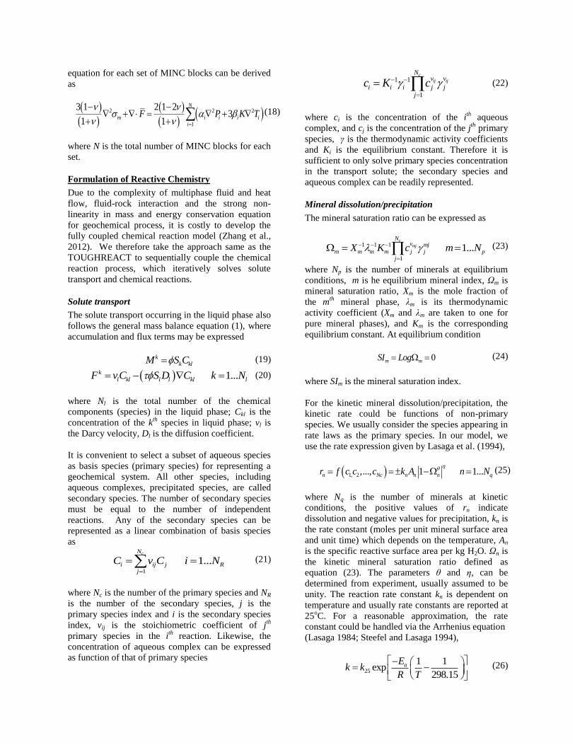
The combined mechanical and chemical effects with
respect to time may be further illustrated as figure 6.
It shows the mechanical and chemical states as
Albite-low 0.18
Muscovite 0.16
Quartz 0.14
Calcite 0.13
Clinochlore-7A 0.08
Illite 0.05
Anorthite 0.02
Clinozoisite 0.01
Unreactive 0.23
16
20
24
28
32
0 50 100 150 200
Mea
n e
ffec
tive
str
ess
(MP
a)
Radial distance (m)
1 day 10days 40 days100days 200 days 365 days
0E+0
5E-4
1E-3
2E-3
2E-3
3E-3
3E-3
4E-3
4E-3
5E-3
5E-3
0 50 100 150 200
Ch
ange
of
min
eral
fra
ctio
n
Radial distance (m)
1 day 10 days 40 days
100 days 200 days 365 days
function of time for one grid block close to the well.
The mean effective stress decreased immediately at
the beginning with negligible change at the later time,
while the chemical precipitation keeps the nearly
constant rate throughout the study time.
Figure 6: The M and C effects on the grid block close
to the wellbore
The induced fracture aperture changes due to
mechanical and chemical effect are calculated from
the parameters in table 1 and plotted as figure 7. The
decreasing effective stress leads to the enhancement
on the facture but the mineral scaling counteracts this
effect. At the early time the stress enhanced aperture
outperforms the chemical precipitation, accordingly
the total change of aperture Δb is positive until 40
days. As analyzed before, mechanical process only
dominates at the early time, the enhanced aperture
decrease from the starting time due to stable
precipitation process. Consequently the change of
aperture becomes negative, less than the initial size of
aperture, in the intermediate and late time. On the
other hand, the chemical effect acts on closer area
and mechanical effect on the further area, which
explains the aperture sharp decrease around the well
and fracture enhancement still exists at the radius of
more than 30m after one year THMC process.
Figure 7: Fracture aperture evolution due to M and
C effects
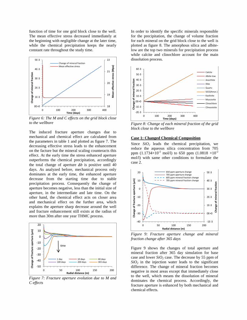
In order to identify the specific minerals responsible
for the precipitation, the change of volume fraction
for each mineral on the grid block close to the well is
plotted as figure 8. The amorphous silica and albite-
low are the top two minerals for precipitation process
while calcite and clinochlore account for the main
dissolution process.
Figure 8: Change of each mineral fraction of the grid
block close to the wellbore
Case 1: Changed Chemical Composition
Since SiO2 leads the chemical precipitation, we
reduce the aqueous silica concentration from 705
ppm (1.1734×10⁻²
mol/l) to 650 ppm (1.0818 ×10⁻²
mol/l) with same other conditions to formulate the
case 2.
Figure 9: Fracture aperture change and mineral
fraction change after 365 days
Figure 9 shows the changes of total aperture and
mineral fraction after 365 day simulation for base
case and lower SiO2 case. The decrease by 55 ppm of
SiO2 in the injection water leads to the significant
difference. The change of mineral fraction becomes
negative in most areas except that immediately close
to the well, which means the dissolution of mineral
dominates the chemical process. Accordingly, the
fracture aperture is enhanced by both mechanical and
chemical effects.
18
19
20
21
22
0E+0
1E-3
2E-3
3E-3
4E-3
5E-3
0 100 200 300 400M
ean
eff
ecti
ve s
tres
s (M
pa)
Ch
ange
of
min
eral
fra
ctio
n
Time (days)
Change of mineral fraction
Mean effective stress
-50
-40
-30
-20
-10
0
10
20
0 50 100 150 200
Ch
ange
of
frac
ture
ap
ertu
re (μ
m)
Radial distance (m)
1 day 10 days 40 days100 days 200 days 365 days
-2E-3
-1E-3
0E+0
1E-3
2E-3
3E-3
4E-3
5E-3
6E-3
0 100 200 300 400
Ch
ange
of
min
eral
fra
ctio
n
Time (days)
Calcite
Albite-low
Anorthite
Illite
Quartz
SiO2(Amor.)
Kaolinite
Muscovite
Clinochlore
Clinozoisite
-1E-3
0E+0
1E-3
2E-3
3E-3
4E-3
5E-3
-40
-30
-20
-10
0
10
20
0 50 100 150 200
Ch
ange
of
min
eral
fra
ctio
n
Ch
ange
of
frac
ture
ap
ertu
re (μ
m)
Radial distance (m)
650 ppm aperture change705 ppm aperture change605 ppm mineral fraction change705 ppm mineral fraction change
time

Case 2: Reduced temperature
The temperature of the injection water has impacts on
both mechanical and chemical process. The case 2
has the reduced temperature of 120 ºC of the
injection water but with the same chemical
composition as the base case.
Figure 10: Mean effective stress and the change of
mineral fraction after 365 days
Figure 10 shows the mechanical and chemical state
after 365 days by comparing the base case and the
reduced temperature case. The mean effective stress
decreases by 1.5 MPa in the areas within 100m of
radial distance, which could strengthen the enhanced
effects on the fracture aperture. However, the lower
injection temperature also results in larger increase in
the mineral fraction, which means the precipitation
reactions are stronger. Thus the temperature decrease
leads to the different directions on aperture change
for mechanical and chemical effects.
Figure 11: Change of fracture aperture due to
mechanical and chemical effects under reduced
injection temperature after 365 days
Figure 11 compares the change of fracture aperture
between base case and the reduced temperature case.
The left plot shows that the chemical precipitation
results in the significant aperture decrease under
lower injection temperature around the wellbore, less
than 50m, even if the rock deformation could
counteract this effect. However, the mechanical
enhanced aperture could be observed beyond the
radius of 50m in the right plot because the
precipitation is weaker in those areas. The lower
temperature leads to the stronger precipitation,
meanwhile stronger mechanical enhanced aperture.
The precipitation outperforms the mechanical
induction in our example, but it may change for
different values of material parameters, such as
maximum mechanical fracture bm, geometry aperture
available for precipitation bg, and mechanical
constant d in equation (31).
CONCLUSIONS
A coupled THMC simulator has been developed for
simulating the multiphase flow, heat transfer, rock
deformation and chemical reactions in EGS
reservoirs. In the model, fluid and heat flow is fully
coupled with geomechanical model since the mean
normal stress, solved simultaneously with fluid and
heat flow equations. The chemical reaction model is
sequentially coupled after the flow equations, solved
at each time step. The solute transport and chemical
reactions are solved iteratively until the chemical
variable converges.
The mechanical model is based on the mean stress
formulation and therefore cannot handle the shear-
stress induced phenomena, such as rock failure by
shearing. But it is sufficient and rigorous to simulate
the stress induced reservoir evolution, such as
porosity and permeability change, formation
subsidence etc.
The application example illustrates the reservoir
evolution in the vicinity areas of the injection well
due to THMC effects. It is found that the mechanical
effects act on the reservoir immediately from the start
and the stress state becomes stable quickly, while the
chemical effects accumulate steadily from beginning
to the intermediate and late time. It is also observed
that the mechanical effects reach further distance
from the injection wells, while the mineral
dissolution and precipitation concentrates around the
injector.
The chemical composition and temperature of
injected water are two key factors influencing the
mechanical and chemical process. By optimizing the
concentration of chemical components of injected
water, the precipitation effects could be minimized or
even eliminated while maintaining the mechanical
enhanced fracture network. The temperature change
has the opposite impacts on the mechanical and
chemical process. For example, the reduced
temperature helps the mechanical enhanced fracture
but leads stronger mineral precipitation. Whether the
0E+0
2E-3
4E-3
6E-3
8E-3
1E-2
1E-2
1E-2
2E-2
2E-2
2E-2
15
17
19
21
23
25
27
29
31
33
0 50 100 150 200ch
ange
of
min
eral
fra
ctio
n
Me
an
eff
ect
ive
str
ess
(M
Pa
)
Radial distance (m)
150 degC effective stress
120 degC effective stress
150 degC change of mineral fraction
120 degC change of mineral fraction
-200
-150
-100
-50
0
50
0 50
Ch
an
ge o
f fr
act
ure
ap
ert
ure
(μm
)
Radial distance (m)
120 degC150 degC
0
1
2
3
4
50 150

temperature change favors or undermines the fracture
network under both mechanical and chemical effects
may also depend on the material properties of the
specific reservoir.
ACKNOWLEDGEMENT
This work is supported by the U.S. Department of
Energy under Contract No. DE-EE0002762,
“Development of Advanced Thermal-Hydrological-
Mechanical-Chemical (THMC) Modeling
Capabilities for Enhanced Geothermal Systems”.
Special thanks are due to the Energy Modeling Group
(EMG) of Department of Petroleum Engineering at
Colorado School of Mines.
REFERENCES
Bai, Mao, and Jean-Claude Roegiers. (1994), "Fluid
flow and heat flow in deformable fractured
porous media." International journal of
engineering science 32, no. 10: 1615-1633.
Davies, J. P., and D. K. Davies. (2001), "Stress-
dependent permeability: characterization and
modeling." SPE Journal, 6.2 : 224-235.
Fakcharoenphol, Perapon, and Yu-Shu Wu. (2011),
"A Coupled Flow-Geomechanics Model for
Fluid and Heat Flow for Enhanced Geothermal
Reservoirs." In 45th US Rock
Mechanics/Geomechanics Symposium.
Jaeger, J. C., N. G. W. Cook, and R. W. Zimmerman.
(2007), “Fundamentals of rock mechanics.”
Blackwell, Fourth edition.
Kiryukhin, A., Xu, T., Pruess, K., Apps, J., &
Slovtsov, I. (2004), “Thermal–hydrodynamic–
chemical (THC) modeling based on
geothermal field data.” Geothermics, 33(3),
349-381.
Lasaga, A. C. (1984), “Chemical kinetics of water-
rock interactions”, J. Geophys. Res., v.89, p.
4009-4025.
Lasaga, A. C., et al. (1994), "Chemical weathering
rate laws and global geochemical cycles."
Geochimica et Cosmochimica Acta, 58.10:
2361-2386.
McKee, C. R., A. C. Bumb, and R. A. Koenig.
(1988), "Stress-dependent permeability and
porosity of coal and other geologic
formations." SPE formation evaluation, 3.1:
81-91.
Montalvo, F., Xu, T., & Pruess, K. (2005),
“TOUGHREACT Code Applications to
Problems of Reactive Chemistry in
Geothermal Production-injection Wells. First
Exploratory Model for Ahuachapán and Berlín
Geothermal Fields.” In Proceedings of World
Geothermal Congress 2005 Antalya, Turkey.
Narasimhan, T. N., and P. A. Witherspoon. (1976),
"An integrated finite difference method for
analyzing fluid flow in porous media." Water
Resources Research, 12.1: 57-64.
Ostensen, R. W. (1986), "The effect of stress-
dependent permeability on gas production and
well testing." SPE Formation Evaluation, 1.3:
227-235.
Pruess, K., Oldenburg, C., and G. Moridis, (1999),
“TOUGH2 user's guide, Version 2.0,”
Lawrence Berkeley Laboratory Report LBL-
43134, Berkeley, CA.
Pruess, K. and T.N. Narasimhan. (1985), “A Practical
Method for Modeling Fluid And Heat Flow in
Fractured Porous Media,” Soc. Pet. Eng. J.,
25, 14-26.
Rutqvist, J., Y-S. Wu, C-F. Tsang, and G.
Bodvarsson. (2002), "A Modeling Approach
for Analysis of Coupled Multiphase Fluid
Flow, Heat Transfer, and Deformation in
Fractured Porous Rock." International Journal
of Rock Mechanics and Mining Sciences 39,
no. 4: 429-442.
Snow, David T. (1969), "Anisotropies permeability
of fractured media." Water Resources
Research 5.6: 1273-1289.
Steefel, C. I., and Lasaga, A. C. (1994), “A coupled
model for transport of multiple chemical
species and kinetic precipitation/dissolution
reactions with applications to reactive flow in
single phase hydrothermal system.” Am. J.
Sci., v. 294, p. 529-592.
Takeno, Naoto, Tsuneo Ishido, and JW. Pritcheit.
(2000), "Dissolution, transportation, and
precipitation of silica in geothermal systems."
Rep Geol Surv Jpn 284 :235-248.
Taron, Joshua, Derek Elsworth, and Ki-Bok Min.
(2009), "Numerical simulation of thermal-
hydrologic-mechanical-chemical processes in
deformable, fractured porous media."
International Journal of Rock Mechanics and
Mining Sciences, 46, no. 5: 842-854.
Tsang, Chin-Fu. (1999), "Linking Thermal,
Hydrological, and Mechanical Processes in
Fractured Rocks 1." Annual review of earth
and planetary sciences 27, no. 1 359-384.
Wang, Xiaonan, and Ahmad Ghassemi. (2012), "A
3D THERMAL-POROELASTIC MODEL
FOR GEOTHERMAL RESERVOIR
STIMULATION." PROCEEDINGS, Thirty-
Seventh Workshop on Geothermal Reservoir
Engineering Stanford University, Stanford,
California.
Winterfeld, P.H., Wu, Y.S. (2011), “Parallel
simulation of CO2 sequestration with rock
deformation in saline aquifers.” Society of
Petroleum Engineers, SPE 141514.
Witherspoon, P. A., J. S. Y. Wang, K. Iwai, and J. E.
Gale. (1979), "Validity of cubic law for fluid
flow in a deformable rock fracture." Technical
Rep. No. LBL-9557, SAC 23.
Xu, T., Ontoy, Y., Molling, P., Spycher, N., Parini,
M., & Pruess, K. (2004a), “Reactive transport
modeling of injection well scaling and
acidizing at Tiwi field, Philippines.”
Geothermics, 33(4), 477-491.
Xu, Tianfu, Eric Sonnenthal, Nicolas Spycher, and
Karsten Pruess. (2004b), “TOUGHREACT
User's Guide: A Simulation Program for Non-
isothermal Multiphase Reactive Geochemical
Transport in Variably Saturated Geologic
Media.” V1. 2.1. No. LBNL-55460-2004.
Ernest Orlando Lawrence Berkeley National
Laboratory, Berkeley, CA (US).
Zhang, Ronglei, Xiaolong Yin, Yu-Shu Wu, and
Philip Winterfeld. (2012) "A Fully Coupled
Model of Nonisothermal Multiphase Flow,
Solute Transport and Reactive Chemistry in
Porous Media." In SPE 2012 Annual Technical
Conference and Exhibition.