countywide assessment of existing & future pavement …dpw.lacounty.gov/gmed/slsr2/octa needs...

Nichols Consulting Engineers, Chtd. Engineer ing and Envi ronmenta l Serv ices 7071 Warner Ave. , #F147

Hunt ington Beach, CA 92647 Phone 714-848-8897 Fax 714-848-2667

FINAL REPORT

Countywide Assessment of Existing

& Future Pavement Needs

Orange County Transportation Authority550 South Main Street

P.O. Box 14184 Orange, CA 92863-1584

March 2006

108.05.30

Submitted to:

Nichols Consulting Engineers, Chtd. Page 1

Table of Contents

Executive Summary ........................................................................................................... 2 1. Overview ...................................................................................................................... 4

Streets & Roads Network........................................................................................................4 Goods Movement....................................................................................................................4 Measure M ..............................................................................................................................6 Pavement Conditions and Thresholds ....................................................................................6 Pavement Condition - 1998 and 2005.....................................................................................7 Objectives of 2005 Study ........................................................................................................8

2. Data Collection........................................................................................................... 10

Pavement Management Data ...............................................................................................10 Pavement Mileages...................................................................................................11

Revenue Data .......................................................................................................................12 3. Maintenance Needs Analyses.................................................................................. 14

Pavement Condition Index (PCI)...........................................................................................14 Performance Curves for Projecting Conditions .....................................................................14 Comparisons of Pavement Condition - 1998 & 2005 ............................................................15 Comparisons of Pavement Condition with Other Agencies...................................................16 Unit Costs of Maintenance Treatments.................................................................................17 Comparisons of Unit Costs - 1998 and 2005 .......................................................................18 Thresholds for Maintenance Treatments ..............................................................................19 Analysis Period and Escalation Factors................................................................................20 Results of Future Maintenance Needs Analyses ..................................................................21

4. Projections of Pavement Expenditures ................................................................... 25

Pavement Expenditure Projections .......................................................................................27 Projected Shortfalls ...............................................................................................................29 Return on Investment............................................................................................................30

5. Summary and Recommendations ............................................................................ 31

Recommendations ................................................................................................................33 Appendix A. Revenue Survey


Executive Summary This study builds upon the previous county-wide assessments that were prepared in 1998. The objectives are to update the results from the 1998 studies, and specifically, to determine the:

Current status of Orange County pavement conditions. Pavement maintenance needs in monetary terms given different pavement condition

goals (i.e. maintain current condition (PCI = 75), and to improve it to 1998 levels (PCI = 81)).

Amount local jurisdictions are spending each year on pavement maintenance activities Project countywide funding shortfalls between projected expenditures and maintenance

needs. Impact on pavement conditions due to the potential loss of Measure M funds.

Pavement condition data were received from 33 out of 35 agencies, and revenue data from 28 agencies. Pavement Condition The current average county-wide pavement condition is a PCI of 75, a reduction from the 1998 estimate of 81. The deterioration is more pronounced for residential/local streets than for arterials/collectors, indicating that there is more investment in arterials/collectors. Reasons for the deterioration are a combination of the weak economic situation in the past 5 years that have diverted more local funds to arterials/collectors and higher than expected maintenance costs. Pavement Expenditures Pavement expenditure data for the past five years (FY 1999-00 to 2003-04) were obtained and the results indicated that agencies relied heavily on Gas Tax subventions and Measure M funds for repairs (46.8%). A third of all transportation revenues were spent on pavements, with the bulk on overlays (19.2%) and reconstruction (59%). The survey data were used to project pavement expenditures for the next 15 years. It was assumed that Measure M sunsets in 2011 and that approximately 32% of Prop. 42 funds are expended on pavements. This results in projected expenditures of $1.326 billion over the next 15 years. Maintenance Needs and Shortfalls Three scenarios were analyzed: Scenario 1: Assuming that the current PCI of 75 is maintained, the countywide pavement maintenance needs are estimated to be $1.64 billion over the next 15 years. The resulting funding shortfall is $314 million. Scenario 2: To improve the pavement condition to 1998 levels (i.e. PCI of 81), the maintenance needs are approximately $2.09 billion over the next 15 years (assuming an annual budget of


$139.3 million/year) or $1.831 billion (assuming no annual budget constraints). The resulting funding shortfall is $764 million and $505 million, respectively. Scenario 3: Given the existing level of pavement expenditures, it is projected that the overall condition will deteriorate to a PCI of 69 by FY 2019-2020. A funding shortfall will result once Measure M sunsets, regardless of the pavement condition goal desired (either PCI = 75 or 81). Therefore, we strongly recommend that OCTA support renewal of Measure M in order to guarantee a stable and consistent source of funds. Renewal of Measure M will provide additional funding; however, alternative funding sources must also be identified in order to achieve the desirable pavement goals. Pavement Management Systems There are a variety of pavement management software utilized by the agencies within Orange County which add to the challenge of performing regional projections. As a minimum, we recommend that OCTA consider the following:

1. Require that agencies include all streets within the pavement management databases. 2. Ensure that all agencies employ a consistent 1-100 scale in rating their pavements and

move away from subjective descriptions. 3. Employ standard procedures to determine maintenance unit costs.

Although this was not an objective in our study, we also recommend that OCTA explore the option of using one standard pavement management software to allow greater ease in future regional projections. Alternative Pavement Rehabilitation Techniques In discussions with the many agencies throughout this study, it was apparent that most employed conventional pavement rehabilitation techniques i.e. slurry seals, conventional asphalt concrete overlays or reconstruction. Alternative pavement rehabilitation strategies are available that can be more cost-effective, and we strongly recommend that longer life designs and the use of alternative materials be considered.


1. Overview The 2000 census data shows that Orange County’s population reached 2.87 million1, making it the second most populated county in California (after Los Angeles County), and the fifth most populated county in the U.S. If it were a city, it would rank fourth largest in terms of population, and larger than the cities of Houston, Philadelphia, Phoenix, San Diego and Dallas. Within Orange County, the two largest cities are Santa Ana and Anaheim (with populations over 300,000 each), and the three smallest are Villa Park, Los Alamitos and La Palma (population less than 20,000). Between 2000 and 2030, Orange County is expected to add another 735,000 people, an increase of 26%. As the County grows, there will be greater demands on the transportation system. The following sections provide a snapshot of the existing streets and roads network as well as an overview of Measure M and its impact.

Streets & Roads Network Orange County’s streets and roads network is composed of approximately 6,542 centerline miles, of which 1,381 centerline miles comprise arterial highways (designated as MPAH, or Master Plan of Arterial Highways), and another 5,161 centerline miles of local streets. (Note that this does not include freeways). The MPAH system carries a little over half the vehicle miles traveled (VMT) in the County and consists of a network of major thoroughfares composed of transportation corridors, arterials and collectors. The completed MPAH will consist of 1,491 centerline miles (6,896 lane miles), and it is projected that $2 billion will be required to complete buildout1. Figure 1.1 illustrates the extent of the MPAH network in Orange County.

Goods Movement Freight volumes in Southern California have been steadily increasing, fueled by the demands of a growing population, economic growth, increased globalization and reduced trade restrictions. It is projected that freight movement will grow by over 80% between 1995 and 20202. Forecasts suggest that heavy-duty traffic will grow by 65% alone. Trucking activity is generally focused in areas where commodities are picked up and delivered, including industrial areas with manufacturing, warehousing and truck terminals. The portions of Orange County with a high concentration of such industrial land uses are areas along I-5, Route 91, SR 57 and other more scattered areas.

1 Directions 2030 – Beyond the Power of Ten: Orange County Long-Range Transportation Plan, 2002. 2 Southern California Freight Management Case Study, Southern California Association of Governments, Caltrans and the Los Angeles County Metropolitan Transportation Authority, 2002.

Figure 1.1 Orange County Arterial Highways (Courtesy OCTA)


The impacts of trucks on pavements are significant and pavement deterioration is directly related to the number of trucks. On arterials, trucking activity is greatest during the peak and midday time periods because of restricted delivery hours. During peak period hours, arterials with relatively high truck volumes carry over 8% large (3+ axles) trucks and up to 46% total trucks (2 or more axles). Typically, urban arterials in Orange County carry no more than 2-3 % large trucks3. The North American Free Trade Agreement (NAFTA) alone is projected to result in an increase of 2,100 additional truck trips per day on the MPAH3.

Measure M In 1990, Orange County taxpayers approved Measure M, a ½ cent sales tax devoted to transportation improvements. This initiative, which will sunset on March 31st, 2011, is expected to provide more than $4.2 billion over 20 years for much needed freeway and local streets and roads improvements. As of March 2005, $361 million has been returned to local agencies as part of Measure M’s Turnback program. An additional $488 million has been allocated through April 2005 on a competitive basis. This is a total of $849 million since inception. When Measure M sunsets in 2011, the result is an expected loss of $234 million annually4. A more detailed analysis of the financial impacts of Measure M is included in Chapter 4.

Pavement Conditions and Thresholds In 1998, the Orange County Transportation Authority (OCTA) performed two county-wide studies5,6; the first assessed the pavement conditions countywide, and the second recommended a standard method for local agencies to assess and report pavement conditions. In the 1998 reports, there was a detailed description of pavement condition and how it is used by local agencies. To briefly recapitulate, pavement condition or quality is used to determine the most appropriate maintenance or rehabilitation strategy. There are a variety of techniques that can be used to determine the pavement condition, but most include an estimation of the type, severity and quantity of distress. This information is then converted into some type of condition index such as Pavement Condition Index (PCI), Pavement Quality Index (PQI) or Condition Score (CS) etc. Depending on the appropriate condition index, a treatment strategy is then assigned. In the first study completed in March 19985, pavement condition data was received from 18 cities (out of 31 incorporated cities and the County) and then extrapolated to the rest of the county in order to arrive at an assessment of the pavement needs. The 18 agencies represented 55% of the total centerline mileage in Orange County.

3 OCTA Goods Movement Study, 1998. 4 Measure M Quick Facts, OCTA. 5 “Countywide Pavement Condition Assessment Study” prepared by Nichols Consulting Engineers, Chtd., March 1998. 6 “Orange County PMS Standardization Recommendations” prepared by Nichols Consulting Engineers, Chtd., August 1998.


However, of the 18 agencies, only 4 provided sufficient information on unit costs for maintenance treatments and pavement condition data to generate performance models. These four agencies were selected as case studies, and initial thresholds were determined based on the data received. In a subsequent survey later the same year, data were received from 20 agencies, and the recommended thresholds were modified as shown in Table 1.1 below. These thresholds were then linked to a maintenance strategy, such as overlays or slurry seals.

Table 1.1 Pavement Condition Thresholds from 1998 Studies5,6

OCTA Studies Condition Category March 1998 August 1998 Very Good 90-100 86-100 Good 84-89 75-85 Fair 73-83 60-74 Poor 60-72 41-59 Very Poor 0-59 0-40

The definition of what is a “Very Good” pavement vs. “Fair” etc is highly subjective i.e. different agencies have different definitions of what is “good” or “poor”. In 2005, there are 34 incorporated cities and the County. Of the 35 agencies, we were able to obtain pavement condition data from 30 agencies, and partial data from 2 cities. Only 3 cities did not provide any data, and in these cases, we had to extrapolate from cities that were similar in size. This represents data on almost 93% of the total centerline mileage. All major cities and the county provided some information for this study. Currently, all but one agency use a 0-100 scale. Therefore, for this study, we have focused our efforts on the condition index values rather than the descriptive categories. The analysis in Chapter 3, for instance, only uses the more objective PCI categories rather than the more subjective descriptions.

Pavement Condition – 1998 and 2005 For purposes of comparison between the 1998 studies and 2005, it is useful to retain the subjective ratings. Nonetheless, any conclusions drawn from this comparison must be tempered with the following caveats:

1. The 1998 study included only 55% of the total centerline mileage, whereas in 2005, the data is for 93% of total centerline mileage. Therefore, any comparisons assume that the 1998 data represents countywide conditions.

2. There was a huge range in pavement distresses measured in 1998, and agencies did not always collect the same data. In 2005, there is more standardization in both the distresses calculated and in the calculation of a condition index.


3. Not all cities in 1998 study used a 0 to 100 scale, and therefore conversions had to be made. In 2005, all but one city uses this scale.

Figure 1.2 shows the pavement conditions for 1998 and 2005 for all streets and roads. As can be seen, there appears to be a gradual deterioration in the pavement quality in the intervening 8 years. Very Good to Good streets have shrunk from 55% to 47.8% of the total pavement area. Conversely, Poor to Very Poor streets have grown from 25.8% to 31.4%. Fair streets have remained about the same. Chapter 3 discusses the pavement condition data in more detail, and possible reasons for the deterioration.

Objectives of 2005 Study This study continues to build upon the previous reports by taking the assessment one step further. Now that pavement conditions are standardized, the objective is to determine the overall county-wide deficiencies and to quantify the investment needed to bring those deficiencies to acceptable levels. In addition, this study updates countywide pavement conditions and compares them with the 1998 study. The results of this study will assist OCTA in updating the Long Range Transportation Plan and related funding outlook. With the expiration of the current Measure M in 2011 and the subsequent loss of those transportation funds, it becomes critically important to have accurate data on what the pavement maintenance needs are, and the impacts of the loss of Measure M. Specifically, the objectives of this study were to determine the:


goals (i.e. maintain current condition, and to improve it to 1998 levels) Amount local jurisdictions are investing each year in pavement maintenance activities. Projected countywide funding shortfalls between projected expenditures and

maintenance needs. Impact on pavement conditions due to the potential loss of Measure M funds.

In addition, this study lists pavement management systems in use by individual agencies, and a brief discussion on alternative pavement rehabilitation techniques is included.

This report describes the process in collecting the data necessary, the technical approach used to perform the analyses and our conclusions and recommendations.


2005 Countywide Pavement ConditionsAll Streets & Roads

(Based on Pavement Area)

Very Good, 26.3%

Good, 21.5%

Fair, 20.8%

Poor, 12.7%

Very Poor, 18.7%

Figure 1.2 Countywide Pavement Conditions for 1998 and 2005

1998 Countywide Pavement ConditionsAll Streets and Roads

(Based on Pavement Area)

Very Good, 36.2%

Good, 18.8%

Fair, 19.2%

Poor, 12.8%

Very Poor, 13.0%


2. Data Collection The pavement network in Orange County is distributed among 34 cities, the County and Caltrans. The 34 cities are: 1. Aliso Viejo 2. Anaheim 3. Brea 4. Buena Park 5. Costa Mesa 6. Cypress 7. Dana Point 8. Fountain Valley 9. Fullerton 10. Garden Grove 11. Huntington Beach 12. Irvine

13. La Habra 14. La Palma 15. Laguna Beach 16. Laguna Hills 17. Laguna Niguel 18. Laguna Woods 19. Lake Forest 20. Los Alamitos 21. Mission Viejo 22. Newport Beach 23. Orange 24. Placentia

25. Rancho Santa Margarita

26. San Clemente 27. San Juan Capistrano 28. Santa Ana 29. Seal Beach 30. Stanton 31. Tustin 32. Villa Park 33. Westminster 34. Yorba Linda

Pavement Management Data All 34 cities and the County utilized some form of pavement management system. Each agency was contacted by OCTA to provide their pavement management system (PMS) database and/or relevant reports for analysis. As part of this study, NCE was able to obtain at least some pavement management data from all but two cities – Garden Grove and La Palma. In the case of Garden Grove, the City apparently does utilize the MicroPAVER pavement management system (PMS) software, but their consultant did not provide the database to NCE. For La Palma, no database was available for analysis. A wide range of PMS software is currently being utilized; Table 2.1 summarizes the types of software used today as well as in 1998. Note that there appears to be a trend towards public domain software such as MicroPaver and the Metropolitan Transportation Commission (MTC) PMS. Only one agency reported using in-house software in 2005, compared to 5 in 1998, indicating a trend towards currently available off-the-shelf software. We also contacted individual cities as needed, primarily to clarify issues such as the unit costs used, or on other data elements in the database. Typical questions included:

What Pavement Management software is used? Version? Are all streets included in the database? Only arterials/collectors? How old is the pavement condition data? What type of pavement condition indices are used? What are the thresholds used for selecting maintenance and rehabilitation

treatments? How are unit costs determined? Contract costs only? Include design and overhead? How is future performance predicted? What kind of performance curves?


Table 2.1 Summary of PMS Software Used in 1998 and 2005

No. of Agencies PMS software 1998 2005 Comments

Cartegraph 1 5 One is converting to MicroPAVER In-house software 5 1 Mostly Excel spreadsheets IMS 2 1 InfraManager 1 1 MicroPaver 8 14

Metropolitan Transportation Commission (MTC) 1 5

Orange County PMS, V 03 3 Stantec PMA V1.43 3 2 Web Quickbase 1 Others 7 1 Mostly proprietary software Totals 21 34

Notes: Not all agencies responded in 1998. Only 1 agency did not indicate software in 2005.

Pavement Mileages OCTA provided NCE with the total mileage for each agency from the GIS database as a quick check to ensure that all pavements were included in the databases. The GIS database is based on data from Thomas Brothers Maps. There were differences between what the agencies reported and what OCTA provided to us. In some cases, it was because the agency did not include any data for residential streets. Since there were insufficient resources to examine the differences for each agency in detail, we selected three cities (Aliso Viejo, Costa Mesa and Newport Beach) as case studies. These cities have small to medium networks (in order to facilitate the process) and had significant differences in their mileages (23%, -5% and 23% respectively). Based on this review, the reasons for the discrepancies are as follows:

Privately maintained streets or alleys may not be included in the agency’s database. Many were internal to housing developments/complexes, and while public access is not restricted, they are typically not maintained by the city.

Agencies may break a divided street into 2 sections by direction (e.g. westbound vs. eastbound) for maintenance purposes, but OCTA’s GIS only reports a single centerline lengths unless there are two separate roadbeds (one for each direction.)

Double-counting of intersections (typically within the GIS, but not in PMS database). Other differences may be attributable to miscoding of a facility type.

All analyses in this study are based on the mileage data from the cities and County as this was deemed to be more representative of actual maintenance expenditures. In cases where no data were provided by the agency, then the mileage data from OCTA was used. From the data provided by the Cities and County, there is a total of 6,057 centerline miles compared to 6,542 miles reported by OCTA.


Revenue Data A survey requesting types and sources of revenue data was sent to all Financial Officers and Public Works Directors to determine current sources of funds for pavement rehabilitation. This was followed by a more detailed survey on June 14th, 2005. A total of 28 agencies responded to the survey. Table 2.2 summarizes the data received. Both pavement expenditures and all sources of transportation revenues were requested for the last five fiscal years i.e. FY 1999-00 to FY 2003-04. This was to obtain a more accurate and balanced view of both revenues and expenditures, and to avoid situations where spikes may occur. For instance, a small city may “save up” revenues for 2 years in order to put together a substantial overlay program to encourage lower bid prices. Pavement maintenance and rehabilitation activities and expenditures included:

Crack seals Slurry seals Overlays

Reconstruction Curb and gutter repairs Other items

The bulk of expenditures were on reconstruction and rehabilitation activities (59%). Since this is the most expensive activity, this is not unexpected. Crack and slurry seals accounted for 12.7% of expenditures, indicating a healthy preventive maintenance program. This is the most effective strategy for pavement preservation. Curb and gutters accounted for a significant 7% of all expenditures. Transportation funds came from a wide variety of sources. Gas tax subventions and Measure M together accounted for 46.8% of all funding (25.2 and 21.6%, respectively). General Funds accounted for a significant 16.4%, despite the unfavorable budgetary conditions of the past five years. Chapter 4 describes in more detail our analysis of the revenue data.


Table 2.2 Results of Revenue Surveys*

Actual Expenditures for Pavement Maintenance and Rehabilitation by Fiscal Year TOTALS Pavement Maintenance and Rehabilitation

Activities 1999-00 2000-01 2001-02 2002-03 2003-04 $ %

Crack Seal 672,535

771,025 1,149,587

836,981

366,652 $3,796,780 1.0% Slurry Seal 6,408,701 7,104,182 14,943,427 8,305,578 7,891,209 $44,653,099 11.7% Overlays 9,209,450 15,799,063 20,767,699 13,766,498 13,704,024 $73,246,734 19.2% Reconstruction and Rehabilitation 28,733,943 40,086,438 47,627,539 49,500,899 59,033,258 $224,982,078 59.0% Curb and Gutter Repair 4,228,020 4,775,915 7,091,275 5,431,067 5,222,962 $26,749,239 7.0% Other 1,646,271 1,920,960 1,449,998 1,508,363 1,511,545 $8,037,137 2.1% Totals $50,898,921 $70,457,583 $93,029,525 $79,349,387 $87,729,650 $381,465,066 100.0%

Actual Revenue Received for All Transportation Activities by Fiscal Year TOTALS

Funding Source (Annually) 1999-00 2000-01 2001-02 2002-03 2003-04 $ % STP (Federal) 5,898,227 4,261,602 5,016,877 4,257,328 7,309,235 $26,743,269 2.2% AHRP (Federal RSTP) 4,352,255 7,145,137 12,936,863 12,904,892 17,089,643 $54,428,789 4.5% Gas Tax 55,053,845 60,355,793 58,928,297 65,304,768 62,973,157 $302,615,861 25.2% Proposition 42 20,870,147 8,552,839 7,856,956 306,791 $37,586,733 3.1% Measure M funds 43,016,997 45,207,143 51,358,402 54,876,349 65,838,803 $260,297,694 21.6% Public Facility Fees (PFF) 1,798,282 1,809,167 2,583,309 2,093,563 2,719,872 $11,004,193 0.9% Assessment Districts 8,035,456 64,967,005 72,427,576 4,425,950 26,700,036 $176,556,023 14.7% General Funds 34,122,979 37,765,950 39,675,146 43,894,465 42,107,612 $197,566,152 16.4% CDBG (Community Development Block Grant) 2,635,601 1,704,849 3,713,901 4,522,978 2,868,352 $15,445,681 1.3% Traffic Congestion Relief 2,242 2,158,933 935,284 924,665 24,594 $4,045,718 0.3% Redevelopment Agency Fund (RDA) 1,698,696 2,003,973 2,496,047 2,644,791 2,559,008 $11,402,515 0.9% TEA (Transportation Enhancement Activities) 51,140 736,724 532,515 1,068,737 860,390 $3,249,506 0.3% Other 21,890,502 8,887,682 21,470,846 25,519,268 23,809,721 $101,578,018 8.4% TOTALS $178,556,222 $257,874,104 $280,627,901 $230,294,711 $255,167,214 $1,202,520,152 100.0% *Results are based on responses from 28 agencies


3. Maintenance Needs Analyses Once all the PMS data were collected as described in Chapter 2, it was necessary to establish baseline conditions for comparisons of the pavement data from each agency. The following key data elements have the highest contribution to differences in funding needs, and so were the foci of this study:

Calculation of pavement condition indices Performance curves used for projecting future conditions Unit costs of treatments Thresholds for triggering maintenance and rehabilitation treatments Inflation factors used to project future costs

Each is described in more detail in the following paragraphs.

Pavement Condition Index (PCI) Since the 1998 report established common standards for pavement distresses and a condition index, it was anticipated that most, if not all, agencies would have collected common distresses and used a common condition index. And indeed, this was true for all but two agencies where we received databases. The remainder employed a 0-100 point scale as recommended in the 1998 report. This facilitated the first portion of the analyses i.e. a determination of county-wide conditions. For the two agencies that did not use a 0-100 point scale, we converted them using a linear relationship i.e. a 0-10 scale was automatically multiplied by a factor of 10 to obtain a 0-100 scale. For those agencies that did not have any local or residential streets in their database, they provided us with subjective estimates as to their condition. For those agencies which did not provide us with their database, we assumed that they would be similar to other agencies with a similar-sized network.

Performance Curves for Projecting Conditions In addition, the age of the pavement condition data was considered. The majority of the agencies had data from 2003 or 2004, but there were others that contained older data. In those cases, we had to project their condition data to the same date for a valid comparison. From the databases provided, it was not always clear what type of performance curves were available. In the case of MicroPAVER, a straight line regression was used. For many of the other systems, we were not able to determine the performance curves used, or if they existed. However, we had available performance curves developed by the Metropolitan Transportation Commission (MTC). These curves were developed using actual data from California cities and counties, and have been widely used by more than 200 agencies not just in California, but throughout the United States since the mid-1980’s. They have been widely accepted and MTC uses them to project future long-term pavement conditions and needs for regional studies, similar to that of OCTA’s. Therefore, they were selected as the basis for projecting the pavement condition data.


Comparisons of Pavement Condition – 1998 & 2005 The overall pavement condition has deteriorated since 1998 study as seen in Table 3.1 below. Local or residential streets have deteriorated the most, by more than 7 points.

Table 3.1 Average Countywide Pavement Condition Index Average PCI 1998 2005 All Roads 81.0 75.0

Arterials/Collectors 80.0 75.8 Local Streets 82.0 74.7

As previously noted in Figure 1.2, Very Good to Good streets have shrunk from 55% to 47.8% of the total pavement area. Conversely, Poor to Very Poor streets have grown from 25.8% to 31.4%. Fair streets have remained about the same. The trend is clear – pavement conditions have gradually deteriorated since 1998, and much more so for residentials than for arterials. Cities and the County have been slightly more successful in maintaining and preserving their arterials/collectors compared to residential and local streets. Which leads us to the following question – why have pavement conditions continued to deteriorate when Measure M funds were supposed to help provide better pavement maintenance? Some factors that could explain this are:

1. Arterials/collectors are eligible for more funding and from more sources, whether federal, state or Measure M. Therefore, arterials and collectors are relatively better maintained than local streets. In addition, local agencies have used Measure M turnback and gas tax funds to match competitive grant programs, and this, in turn, reduces funding for local /residential streets.

2. There is an increasing use of gas tax funds for other eligible services, e.g. tree trimming,

street sweeping, median maintenance, etc. This reduces the funds available for pavements.

3. The costs of maintenance may actually be higher than originally estimated, and

therefore estimates of pavement needs may have been too low. This is further explored in the next section.

4. The 2000-2001 national economic recession7 may have adversely affected local funds.

Lingering impacts from the County’s bankruptcy in 1994 may also remain. The state’s fiscal crisis has also had a detrimental impact on local funds, such as the Vehicle License Fee. Gas tax and General Funds are the primary sources for local streets, and yet are most affected by the economic climate.

7 National Bureau of Economic Research, www.nber.org


The next few sections discuss in more detail the factors used in our analysis.

Comparisons of Pavement Condition with Other Agencies An average pavement condition of 75, by itself, may not mean much until we compare this with other agencies. The most comprehensive data on pavement conditions comes from the San Francisco Bay area, where MTC monitors annual pavement conditions for over 100 cities and counties. The Bay area has approximately 19,000 centerline miles of streets and roads. Regionally, the average PCI is 65, which is considerably lower than Orange County. Approximately 44% of the Bay area network has a PCI greater than 75 (considered to be Good to Excellent), 32% have a PCI between 45 and 74 (considered Fair to Good), and 16% have a PCI less than 45 (Poor to Very Poor). Note that the subjective descriptions used are quite different than those used in Orange County. Therefore, a direct comparison with Orange County is not possible because of the different thresholds used. Table 3.2 below summarizes pavement conditions for sample agencies in the Bay area. The full

Table 3.2 Sample Pavement Conditions from Other Cities8

Agency 2002 Average PCICounties (unincorporated areas)

Alameda County 79 Contra Costa County 83 Marin County 54 Napa County 55 San Mateo County 62 Santa Clara County 64 Solano County 66 Sonoma County 50

Cities Berkeley 59 Concord 78 Fairfield 81 Fremont 77 Hayward 69 San Francisco 66 San Jose 66 San Leandro 64 Santa Clara 86 Santa Rosa 66 Vacaville 81

report may be found on the www.mtc.ca.gov website8. The pavement conditions reported are for 2002. Note that the more rural and less populated counties (Napa, Marin, and Sonoma) tend to have lower PCIs. More urban counties like Santa Clara, Alameda and Contra Costa have more similarities to Orange County (since the populations and traffic levels are higher) and some have PCIs that are higher.

8 Bay Area Transportation: State of the System 2004, Metropolitan Transportation Commission, February 2005.


Some sample cities are also included, and again, there is a wide range of PCIs reported. In general, smaller cities that are bedroom communities, or that are growing rapidly will have higher PCIs because of the addition of new streets to the network (e.g. Vacaville or Fairfield). Older cities that are built out will tend to have lower PCIs.

Unit Costs of Maintenance Treatments In the next phase of our analyses, we looked at the unit costs of the treatments assigned. This is a particularly critical component of the analyses since it has a tremendous impact on the maintenance needs calculations. Approximately half of the agencies provided us with unit cost data, and there was a wide range in the unit costs provided for the same treatments (see Table 3.3). To understand the range in costs, we had further discussions with the cities, and found that there were different

Table 3.3 Unit Costs for Maintenance Treatments Unit costs from Cities

($/sy) Unit costs used in analysis

($/sy) PCI Range Maintenance Treatment

Range Average Arterials / Collectors

Residential/Local

Asphalt Concrete Pavements

90-100 Do Nothing $ - $ - 70-90 Surface Seal/Crack Sealing $1.15 - $3.25 $ 1.67 $ 1.90 $ 1.80 70-90 Restoration(1.5" Overlay) $4.23 - $11.70 $ 6.57 $ 8.80 $ 8.20

50-70 Thin Overlay (1.5” - 2" Overlay) $ 11.50 $ 10.70

40-50 Thick Overlay (3.5" Overlay) $6.65 - $23.85 $ 15.29

$ 21.30 $ 19.80 0-40 Reconstruction $9.00 - $74.70 $ 38.17 $ 52.50 $ 34.30 Portland Cement Concrete Pavements 90-100 Do Nothing $ - $ -

70-90 Crack Sealing $1.00/ft $1.00/ft

50-70 Slab repairs* $ 2.00 $ 1.80 40-50 Slab replacement* $ 6.00 $ 5.50 0-40 Reconstruction $ 60.00 $ 52.00 Cities reported a wide range of unit costs. Not all Cities included the same elements in deciding unit costs i.e. contract cost, overhead, engineering design and other related activities. The unit costs used in the analysis were based on:

Engineering estimates 2004 survey from MTC (from 75+ cities); and Cities’ databases.

* Unit cost is applied to entire area of pavement philosophies in determining unit costs. Some cities only included contract costs or material costs, while others included engineering design, overhead, construction testing and inspection and so forth. This was consistent with their uses of the results. In other words, if a city wanted to estimate the costs of a slurry seal contract, then only construction contract costs were included. However, if a city wanted to use the results for budgeting, then engineering and other costs were included.


In order to arrive at a baseline unit cost for treatments, we examined two additional sources of data. The first is the result of a 2004 survey performed by MTC for the 106 cities and counties in the San Francisco Bay area. Over 75% of those cities responded, and this provided us with a rich source of data. While costs in the Bay area can vary from Orange County, nonetheless, this provided us a basis for comparison and with a test of “reasonableness”. The MTC study included fully-loaded unit costs i.e. they included engineering and other costs in addition to materials. This is much more useful for regional planning studies such as this one. The second was an examination of engineering estimates recently performed by NCE for various clients that included projects that were similar to those in the PMS databases. This again provided us with a test of “reasonableness”. The final unit costs selected for our analyses (shown in Table 3.3) included the following elements:

Engineering design Overhead Paving materials Other related costs such as signal loops, striping and other traffic markings Surface preparation activities e.g. base repairs Traffic control Construction testing and inspection Construction management Contingencies

Since the results of this study is intended to be used for long-term budgeting, and to assess the total pavement needs, it was determined that a complete picture is only possible with “fully-loaded” unit costs that include the above elements. Note too that we differentiated between the unit costs for arterial streets vs. collector or residential streets. Typically, arterials will have higher costs (more traffic control requirements, more striping, signals etc). Finally, no unit costs were provided for Portland cement concrete (PCC) pavements; therefore, our projections are based on engineering estimates.

Comparisons of Unit Costs – 1998 & 2005 Table 3.4 is a comparison of the unit prices used in the 1998 study and in 2005. Note that all 1998 costs were adjusted for inflation, and reported in 2005 dollars. This table shows that there have been significant increases in the unit costs in the intervening years. For example, the cost of a thin overlay in 2005 for an arterial is 11% more than estimated in 1998. For reconstruction, the differences are particularly stark. Note too that 59.1% of the expenditures reported in Table 2.2 was for reconstruction, and therefore accounts for a huge portion of the pavement maintenance. On average, the 2005 costs are 17% higher for arterials/collectors, and 19% higher for residentials/locals (for asphalt concrete pavements). In short, construction costs have escalated much more than originally estimated in the intervening years from 1998 to 2005. The escalations can partly be attributed to new state and federal regulatory requirements, such as the addition of ADA (American with Disabilities Act) ramps, NPDES (National Pollutant


Table 3.4 Comparison of Unit Costs – 1998 and 2005

Maintenance & Rehabilitation Unit Costs ($/sy) Differences (%)

1998* 2005 Treatment

Arterials / Collectors

Residential/Local


Residential/Local


Residential/Local

Asphalt Concrete Pavements Slurry Seal $ 2.61 $ 1.54 $ 1.90 $ 1.80 -27% 17% Thin Overlay $ 10.32 $ 8.59 $ 11.50 $ 8.20 11% -5% Thick Overlay $ 16.54 $ 13.47 $ 21.30 $ 19.80 29% 47% Reconstruction $ 34.08 $ 29.19 $ 52.50 $ 34.30 54% 18%

Average Difference 17% 19% Portland Cement Concrete Pavements

Reconstruction $ 56.97 $ 28.38 $ 60.00 $ 52.00 5% 83%

*1998 costs adjusted for inflation, and reported in 2005 dollars. Discharge Elimination System) permits, as well the use of new pavement materials, e.g. rubberized asphalt concrete. All these factors help to explain why Measure M funds have not been able to prevent the deterioration in the pavement condition.

Thresholds for Maintenance Treatments In addition to examining the unit costs, we also looked at the thresholds or triggers for specific treatments. Different agencies have different standards – City A may program an overlay when the PCI is 60 whereas City B may program one when the PCI is at 75. Some cities may program no activity on streets with a high PCI while others may require preventive maintenance. This results in funding needs that are not directly comparable. There is no one correct way to program thresholds. How these thresholds are determined depend on the needs of individual agencies. Typically, there are two approaches to develop these thresholds; by programming what should be done, or by programming what is actually done. The former approach reflects what is required based on engineering or other technical criteria, while the latter reflects budget constraints that eliminate certain choices. The consequences of the latter approach is that the pavement needs are usually understated because it reflects the budget constraints of an agency, and not the real needs. A common example is the replacement of overlays with seals due to inadequate funds. Therefore, for this study, we used the first approach i.e. we programmed thresholds and treatments based on what should be done using generally accepted engineering criteria. This is reflected in Table 3.5 where different maintenance treatments are recommended for different PCI ranges.


Table 3.5 Thresholds for Maintenance Treatments

PCI Ranges Programmed Maintenance Treatments

90-100 Do Nothing

84-89

73-83

70-73

Preventive/Routine Maintenance

60-70 Thin Overlay

40-59 Thick Overlay

0-39 Reconstruction

Analysis Period and Escalation Factors For this study, we looked at a 15 year analysis period, and assumed a 2.5% annual inflation factor. This is based on data for the U.S. Department of Labor9 from 1990 to 2005. In addition, we also examined the escalation in construction costs in transportation. Table 3.6 from Caltrans10 is particularly illuminating.

Table 3.6 Price Index for California Construction Items10

Period Annual Average % Change in Construction Prices

1989 - 2003 2.48% 1990 - 2004 5.07% 1995 - 2004 8.04%

Oct. 2004 - June 2005 22.60%

Although the data for the last 9 months in the table above is particularly startling, it would be unreasonable to assume that an annual increase of 22% can be sustained over the next 15 years. Based on the above data and upon consultation with OCTA, we used an annual average of 5.5% as the most reasonable escalator for construction costs. It should also be noted that within the 15 year period, multiple treatments are projected to occur on any one street. For instance, a street that is overlaid in Year 1 may expect a slurry seal in Year 7 and another in Year 13. Another that has a PCI of 95 in Year 1 will be programmed for preventive maintenance and perhaps a restoration within the 15 year analysis period.

9 U.S. Department of Labor, Bureau of Labor Statistics. www.bls.gov/cpi 10 Caltrans, Division of Engineering Services – Office Engineer. www.dot.ca.gov/hq/esc/oe


Finally, all results are reported in 2005 dollars to be consistent with OCTA’s Long Range Transportation Plan.

Results of Future Maintenance Needs Analyses As indicated in Chapter 1, one of the primary objectives of this study is to determine the maintenance needs. The answer to this question leads to yet another – the maintenance needs at which pavement condition level? In other words, if the desired pavement condition goal is, say, a PCI of 60, then the maintenance needs will be considerably less than if the pavement condition goal is 80. In discussions with OCTA staff and the Technical Steering Committee (TSC) as well as the Technical Advisory Committee (TAC), it was determined that we should look at this question from three different perspectives.

Scenario 1: Maintain current pavement condition (i.e. PCI = 75) Scenario 2: Improve pavement condition to 1998 levels (i.e. PCI = 81) Scenario 3: Impact on pavement condition from loss of Measure M funds after 2011

Each scenario is described in more detail in the following paragraphs. Again, all results are reported in 2005 dollars. Scenario 1: Maintain current pavement conditions The underlying assumption in this scenario was to ensure that the countywide pavement condition levels would remain at its current level of 75. What this also implies is that cities where the average pavement condition is considerably higher than 75 may see a reduction, while those with PCI lower than 75 will see an improvement. However, for purposes of a county-wide study such as this, this is an acceptable assumption. The results of the pavement needs analyses are summarized in Table 3.7 below.

Table 3.7 Summary of 15 year Maintenance Needs

Types of Streets 15 Year Needs

(millions)

Arterials/Collectors $ 800 Residentials/Locals $ 840

Total $ 1,640

The total 15-year maintenance needs are estimated to be $1.64 billion and almost evenly split between arterials/collectors and residentials/locals. On an annual basis, this is approximately $109 million a year. Of course, this assumes that no additional pavements are added within the next 15 years, which may not be a reasonable assumption given the developments in the County. However, these will be new streets and should exhibit excellent pavement conditions, and therefore minimal maintenance needs initially.


Scenario 2: Improve pavement conditions to 1998 levels In this scenario, we determined the funds needed to improve the pavement conditions to 1998 levels (i.e. PCI = 81), or to put it another way, the maintenance needs in order to achieve a PCI goal of 81. There are two conceivable ways to achieve this goal:

a. Assume no annual budget constraints i.e. variable expenditures based on PMS projections

b. Assume a stable annual budget. The subtle difference between the two assumptions above is that the first has no budget constraints on an annual basis, so therefore the most cost-effective approach is to perform all repairs in the first year. This results in an extremely large list of repairs in the first few years, and much lower costs in subsequent years. This approach essentially “front loads” the repairs and in doing so, minimizes future repairs. The second is a more realistic scenario, because most agencies would have or prefer to have a consistent budget from one year to the next. This eliminates any spikes in the funds available, allowing agencies to manage a consistent workload with stable labor resources. However, by spreading out the maintenance needs over 15 years, maintenance costs will increase because streets that should have been repaired in Year 2 are deferred until, say, Year 11, and the cost of repair will therefore increase, either because of inflation or because the treatment in Year 2 is no longer appropriate in Year 11. Table 3.8 below summarizes the different funding levels used in the analyses.

Table 3.8 Annual Budgets Used in Maintenance Needs Analyses Annual Budgets ($ million)

Scenario 2 Improve to 1998 Levels Year Scenario 1

Maintain Current PCI Unconstrained

Budget Stable Annual

Budget

Scenario 3 Loss of

Measure M

2005 $ 109.3 $ 665.1 $ 139.3 $ 90.8 2006 $ 109.3 $ 122.1 $ 139.3 $ 86.9 2007 $ 109.3 $ 125.0 $ 139.3 $ 100.5 2008 $ 109.3 $ 102.4 $ 139.3 $ 100.7 2009 $ 109.3 $ 88.5 $ 139.3 $ 100.8 2010 $ 109.3 $ 65.9 $ 139.3 $ 101.0 2011 $ 109.3 $ 38.2 $ 139.3 $ 82.1 2012 $ 109.3 $ 231.0 $ 139.3 $ 82.3 2013 $ 109.3 $ 56.7 $ 139.3 $ 82.4 2014 $ 109.3 $ 34.5 $ 139.3 $ 82.6 2015 $ 109.3 $ 10.1 $ 139.3 $ 82.8 2016 $ 109.3 $ 9.5 $ 139.3 $ 83.0 2017 $ 109.3 $ 33.0 $ 139.3 $ 83.2 2018 $ 109.3 $ 55.6 $ 139.3 $ 83.4 2019 $ 109.3 $ 193.3 $ 139.3 $ 83.6

Totals $ 1,639.5 $ 1,831.0 $ 2,090.1 $ 1,326.0


Overall, Scenario 2a results in a smaller 15 year total pavement expenditure of $1.831 billion, but is probably unrealistic. Scenario 2b is more realistic, but results in a higher 15 year expenditures of $2.09 billion. On an annual basis, this is $139.3 million/year. There is, again, a near even split between the maintenance needs for arterials/collectors and residentials/locals (see Table 3.9 below).

Table 3.9 Summary of 15 year Maintenance Needs

Type of Streets 15 Year Needs

(millions)

Arterials/Collectors $ 1,080 Residentials/Locals $ 1,010

Total $ 2,090

Scenario 3: Loss of Measure M funds In the last scenario analyzed, the question asked was slightly different. Since Measure M is due to sunset in 2011, both the Technical Steering Committee and TAC had the same question – what will be the impact on the pavement condition if Measure M is not renewed? The assumptions we used to determine the annual budgets used in this analysis are:

The baseline is the average pavement expenditures from 1999 to 2004 (this is described in more detail in Chapter 4)

Measure M ends in 2011 and there is no reduction in the MOE (maintenance of effort) levels of approximately $70 m/year.

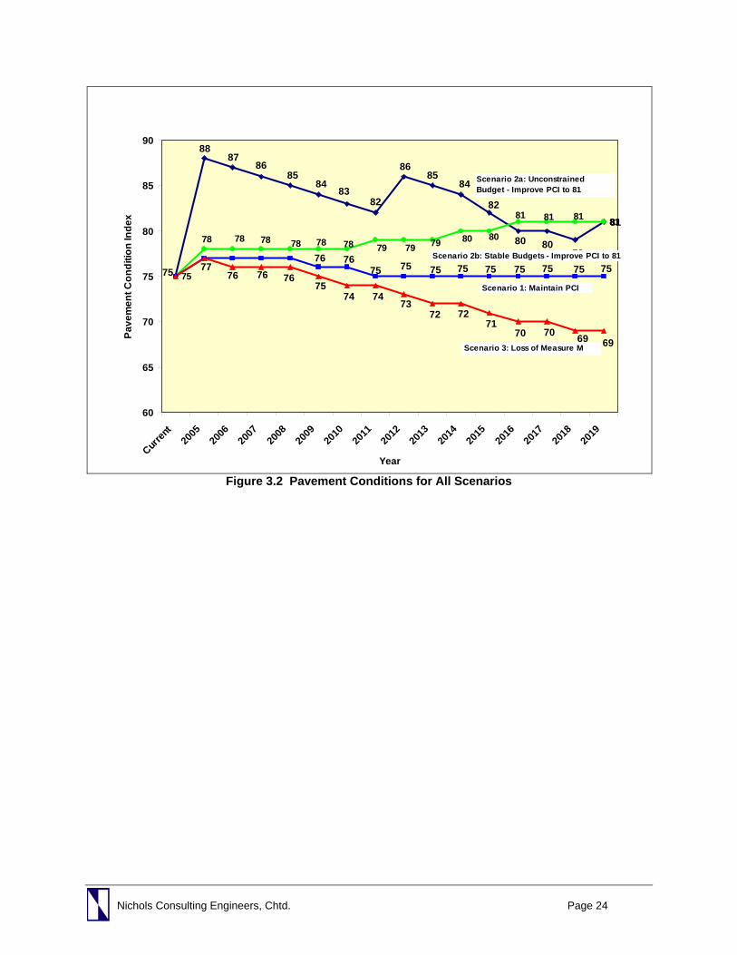
Proposition 42 funds are available for all years except 2006-07. The results indicate a clear trend in the pavement deterioration. By FY 2019-2020, the overall pavement condition index is expected to drop 6 points to 69. Summary of Results Figure 3.2 below illustrates the results in the pavement conditions depending on the scenario. Note again that both Scenarios 2a and 2b arrive at the final PCI of 81 by FY 2019-2020, but achieve this through different means. Scenario 2a, as described earlier, assumes an unconstrained annual budget that allows it to achieve most of the improvements within the first year. Scenario 2b assumes a stable annual budget, which results in gradual improvements.


81

75

81

8887

8685

8483

82

8685

84

82

80 8079

818181

80 80797979787878787878

757575757575757676

75 7575 7776 76 76

7574 74

7372 72

7170 70 69 69

60

65

70

75

80

85

90

Curren

t20

0520

0620

0720

0820

0920

1020

1120

1220

1320

1420

1520

1620

1720

1820

19

Year

Pave

men

t Con

ditio

n In

dex

Scenario 2a: Unconstrained Budget - Improve PCI to 81

Scenario 2b: Stable Budgets - Improve PCI to 81

Scenario 1: Maintain PCI

Scenario 3: Loss of Measure M

Figure 3.2 Pavement Conditions for All Scenarios


4. Projections of Pavement Expenditures As previously mentioned in Chapter 1, a revised revenue survey was sent out to all agencies on June 14th, 2005. Agencies were requested to identify their actual pavement expenditures over a five-year period (1999 to 2004). A multi-year period was requested to ensure that any peaks or valleys in funding could be identified. For instance, many smaller agencies budget for an overlay program only every 2 years. The fluctuations in the state budget have also affected local budgets, so it was desirable to determine as accurately as possible the average funds annually. Pavement maintenance and rehabilitation activities included:

Crack seals Slurry or other surface seals Overlays

Reconstruction Curb and gutter repairs Other activities

The types of funding sources included:

Federal (STP and RSTP) Gas taxes Proposition 42 Measure M Public Facility fees Assessment districts Special maintenance districts

General Funds Community Development Block

Grants Traffic Congestion Relief Redevelopment Agency Transportation Enhancement

Activities Of the 35 agencies surveyed, a total of 28 responded. The results were summarized in Table 2.2 and reproduced here as Table 4.1. The top half of Table 4.1 represent the pavement expenditures of the agencies. The bottom half represent the revenues received for all transportation activities including traffic signals, bridges, safety projects, pedestrian, bicycle projects etc. Since pavement maintenance is only a small portion of the total transportation activities, we would expect to see more revenues than pavement expenditures. Overall, pavement expenditures are a significant portion of total transportation revenues i.e. approximately 32%. Of this, 59% is spent on reconstruction and rehabilitation activities, with an additional 19.2% on overlays. Preventive maintenance accounts for 12.7%, a very cost-effective strategy for pavement preservation.

The majority of transportation funds come from two main sources: Gas tax subventions and Measure M. While the former is expected, it was with some surprise that to see that agencies relied so heavily on Measure M funds (21.6% of total revenues).The next two primary sources of funds were General Funds and Assessment Districts (31.1% combined). However, funds from Assessment Districts appear to be extremely volatile i.e. $8 million in 1999-00, then jumping to $65 million the next year, $73 million the following year, and then abruptly dropping to $4 million the year after before rebounding to $26 million in 2003-04. One encouraging feature is that most agencies are continuing to use General Funds for transportation activities. Of the 28 agencies reporting, 16 report that General Funds are available for transportation. However, this could also be due to the maintenance of effort (MOE)


Table 4.1 Summary of Revenue Surveys*

Actual Expenditures for Pavement Maintenance and Rehabilitation by Fiscal Year TOTALS Pavement Maintenance and Rehabilitation

Activities 1999-00 2000-01 2001-02 2002-03 2003-04 $ %

Crack Seal 672,535

771,025 1,149,587

836,981

366,652 $3,796,780 1.0% Slurry Seal 6,408,701 7,104,182 14,943,427 8,305,578 7,891,209 $44,653,099 11.7% Overlays 9,209,450 15,799,063 20,767,699 13,766,498 13,704,024 $73,246,734 19.2% Reconstruction and Rehabilitation 28,733,943 40,086,438 47,627,539 49,500,899 59,033,258 $224,982,078 59.0% Curb and Gutter Repair 4,228,020 4,775,915 7,091,275 5,431,067 5,222,962 $26,749,239 7.0% Other 1,646,271 1,920,960 1,449,998 1,508,363 1,511,545 $8,037,137 2.1% Totals $50,898,921 $70,457,583 $93,029,525 $79,349,387 $87,729,650 $381,465,066 100.0%

Actual Revenue Received for All Transportation Activities by Fiscal Year TOTALS

Funding Source (Annually) 1999-00 2000-01 2001-02 2002-03 2003-04 $ % STP (Federal) 5,898,227 4,261,602 5,016,877 4,257,328 7,309,235 $26,743,269 2.2% AHRP (Federal RSTP) 4,352,255 7,145,137 12,936,863 12,904,892 17,089,643 $54,428,789 4.5% Gas Tax 55,053,845 60,355,793 58,928,297 65,304,768 62,973,157 $302,615,861 25.2% Proposition 42 20,870,147 8,552,839 7,856,956 306,791 $37,586,733 3.1% Measure M funds 43,016,997 45,207,143 51,358,402 54,876,349 65,838,803 $260,297,694 21.6% Public Facility Fees (PFF) 1,798,282 1,809,167 2,583,309 2,093,563 2,719,872 $11,004,193 0.9% Assessment Districts 8,035,456 64,967,005 72,427,576 4,425,950 26,700,036 $176,556,023 14.7% General Funds 34,122,979 37,765,950 39,675,146 43,894,465 42,107,612 $197,566,152 16.4% CDBG (Community Development Block Grant) 2,635,601 1,704,849 3,713,901 4,522,978 2,868,352 $15,445,681 1.3% Traffic Congestion Relief 2,242 2,158,933 935,284 924,665 24,594 $4,045,718 0.3% Redevelopment Agency Fund (RDA) 1,698,696 2,003,973 2,496,047 2,644,791 2,559,008 $11,402,515 0.9% TEA (Transportation Enhancement Activities) 51,140 736,724 532,515 1,068,737 860,390 $3,249,506 0.3% Other 21,890,502 8,887,682 21,470,846 25,519,268 23,809,721 $101,578,018 8.4% TOTALS $178,556,222 $257,874,104 $280,627,901 $230,294,711 $255,167,214 $1,202,520,152 100.0% *Results are based on responses from 28 agencies


requirements for Measure M, which states that the minimum annual level of local streets and roads expenditures shall be based upon an average of the expenditures over the five years from FY 1985/86 to FY 1989/90. As a side note, MOE eligible expenditures include street lights, traffic signals, landscaping and not necessarily just pavement rehabilitation and maintenance. Two cities, Aliso Viejo and Rancho Santa Margarita, did not have complete data for the entire 5 year period since they were only incorporated in 2001. In this case, only the data from the last two years (2002-03 and 2003-04) are used in this analysis.

Pavement Expenditure Projections In order to determine the funding shortfall, we projected the anticipated expenditures for pavement maintenance and rehabilitation based on current levels of expenditures. We looked at a 15 year analysis period; from 2005-06 to 2019-20. Annual Growth Rates The annual growth rates were calculated from Table 4.1 and summarized below in Table 4.2.

Table 4.2 Summary of Growth Rates in Expenditures and Revenues

Period

Growth in Pavement

Expenditures

Growth in Transportation

Revenues 1999-00 to 2000-01 38% 13% 2000-01 to 2001-02 32% 8% 2001-02 to 2002-03 -15% 8% 2002-03 to 2003-04 11% -1%

Average 17% 8% The average growth in pavement expenditures is 17%. However, the growth rate for the revenues is much lower, only 8% (note that funds from Assessment Districts were not included because of their volatility). There is also a downward trend in the revenues reported from 2002 to 2004. However, future projections of expenditures are not dependent on historical trends. From the surveys, pavement expenditures depend highly on two key funding sources, Measure M and Proposition 42. Both are discussed in more detail in the following paragraphs. Measure M Because Measure M sunsets in 2011, all revenue projections from 2011-12 to 2019-20 do not include any Measure M revenues. It should be noted that Measure M was intended to supplement and not replace existing local revenues, which have been traditionally used for local street and maintenance improvements.


Further, as was described earlier, the Measure M maintenance of effort (MOE) requirement states that the minimum annual level of local streets and roads expenditures shall be based upon an average of the expenditures over the five years from FY 1985/86 to FY 1989/90. Currently, this is approximately $70 million a year. There is a possibility that if Measure M were to end, then the MOE requirement may also be reduced. Proposition 42 With recent passage of the State’s budget, Prop. 42 funds are again available to local agencies. For FY 2005-06, it is anticipated that Orange County will receive approximately $20 million in 2005-06 and this slowly increases to an annual level of $57 million by 2019-202011. Table 4.3 below lists the additional funds available from Proposition 42.

Table 4.3 Summary of Projected Pavement Expenditures

Year Baseline

Expenditures ($ million)

Additional Prop. 42 Funds

($ million)

Total ($ million)

2005-06 $ 86.9 $ 3.9 $ 90.8 2006-07* $ 86.9 $ - $ 86.9 2007-08** $ 86.9 $ 13.6 $ 100.5 2008-09 $ 86.9 $ 13.8 $ 100.7 2009-10 $ 86.9 $ 13.9 $ 100.8 2010-11 $ 86.9 $ 14.1 $ 101.0 2011-12 $ 67.9 $ 14.2 $ 82.1 2012-13 $ 67.9 $ 14.4 $ 82.3 2013-14 $ 67.9 $ 14.5 $ 82.4 2014-15 $ 67.9 $ 14.7 $ 82.6 2015-16 $ 67.9 $ 14.9 $ 82.8 2016-17 $ 67.9 $ 15.1 $ 83.0 2017-18 $ 67.9 $ 15.3 $ 83.2 2018-19 $ 67.9 $ 15.5 $ 83.4 2019-20 $ 67.9 $ 15.7 $ 83.6 Totals $ 1,132 $ 194 $ 1,326

Assumptions Baseline expenditures are based on survey data. Only 32% of Prop. 42 funds are assumed available for pavements. * For FY 2006-07, agencies may receive Prop. 42 funds owed from previous years. ** For FY 2007-08, agencies are likely to receive less than full funding for Prop. 42

The assumptions made for the above projections were:

Measure M end in 2010-2011. There is no reduction in Measure M MOE funds. Only 32% of Prop. 42 funds would be spent on pavement expenditures.

11 Proposition 42 projections provided by OCTA, October 2005.


In order to be eligible for Prop. 42 funds, there is also a MOE requirement which states that cities and counties shall maintain their existing commitment of local funds for street and highway maintenance, rehabilitation, reconstruction, and storm damage repair in order to remain eligible for these funds. Any city or county that is not in compliance would be required to reimburse the state for funds received during that fiscal year. The level of required expenditure will be based on the city or county’s average annual expenditures from its general funds for the fiscal years 1996-97, 1997-98, and 1998-99. Note too that pursuant to Senate Bill 460, chapter 716 (2003 Statutes), cities and counties were not required to meet the MOE for fiscal years during which Prop. 42 payments were not received from the state. This is significant because all cities and counties will be entitled to Prop. 42 payback from the state, without consideration paid to the MOE requirement.

Projected Shortfalls To determine the funding shortfalls, we compared the projected expenditures with the maintenance needs calculated in Chapter 3. Table 4.4 below summarizes the results:

Table 4.4 Summary of 15 Year Analysis 15 year Projections

Scenarios Pavement

Expenditures ($ million)

Maintenance Needs

($ million) Shortfall

($ million)

Scenario 1: Maintain Current PCI Total without Prop. 42 $ 1,132 Est. Additional Prop. 42 Funds $ 194

Total with Prop. 42 $ 1,326 $ 1,640 $ (314) Scenario 2a: Improve to 1998 Levels (Unconstrained budget)

Total without Prop. 42 $ 1,132 Est. Additional Prop. 42 Funds $ 194

Total with Prop. 42 $ 1,326 $ 1,831 $ (505) Scenario 2b: Improve to 1998 Levels (Stable budget)

Total without Prop. 42 $ 1,132 Est. Additional Prop. 42 Funds $ 194

Total with Prop. 42 $ 1,326 $ 2,090 $ (764) As can be seen, even under the most minimal conditions (i.e. Scenario 1: Maintain current conditions), there is a $314 million shortfall. To conclude, it should be noted that the pavement expenditures are for the current pavement network, and does not include new streets and roads that may be added in the future. A 5% growth in the pavement network alone is approximately 300 miles and would have a significant impact on pavement expenditures.


Return on Investment Another way to look at the results of our analysis is to examine the graph (Figure 4.1) below. The same data can be presented in terms of the return on investment (dashed lines are extrapolations).

Figure 4.1 Return on Investment For instance, at the current projected expenditures of $1.326 billion (see red lines), the resulting pavement condition is 69 at the end of 15 years. However, if the same expenditures were to be spread out over 20 years, the resulting condition would be 56.5. Finally, if we were to maintain the pavement network at its current PCI of 75 (see light blue lines), it would require an investment of $ 1.093 billion over 10 years, or $1.64 billion over 15 years, or $2.187 billion over 20 years.

50

55

60

65

70

75

80

85

90

$- $0.50 $1.00 $1.50 $2.00 $2.50 $3.00

Cumulative Investment ($Billion)

After 1 Year After 5 Years After 10 Years

After 15 Years After 20 Years

$2.187$1.640$1.093 $1.326

79

69

56.5

Resulting Average Network Pavement Condition


5. Summary and Recommendations The objectives of this study were to determine the:


goals (i.e. maintain current condition, and to improve it to 1998 levels) Amount local jurisdictions are spending each year on pavement maintenance activities. Projected countywide funding shortfalls between projected expenditures and

maintenance needs. Impact on pavement conditions due to the potential loss of Measure M funds.

In addition, this study was to make recommendations regarding the pavement management systems in use by individual agencies, and to include a brief discussion on alternative pavement rehabilitation techniques. Pavement condition data were received from 33 out of 35 agencies, and revenue data from 28 agencies. This is a vast improvement over the data received for the 1998 studies. Pavement Condition The current average county-wide pavement condition is a PCI of 75, a reduction from the 1998 estimate of 81. The deterioration is more pronounced for residential/local streets than for arterials/collectors, indicating that there is more investment in arterials/collectors. Reasons for the deterioration are a combination of the weak economic situation in the past 5 years that have diverted more local funds to arterials/collectors and higher than expected maintenance costs. Pavement Expenditures Pavement expenditure data for the past five years (FY 1999-00 to 2003-04) were obtained and the results indicated that agencies relied heavily on Gas tax subventions and Measure M funds for repairs (46.9%). A third of all transportation funds were spent on pavements, with the bulk on overlays (19.2%) and reconstruction (59%). This information was used to project pavement expenditures for the next 15 years. It was assumed that Measure M sunsets in 2011 and that approximately 32% of Prop. 42 funds are used for pavements. This results in projected expenditures of $1.326 billion over the next 15 years. Maintenance Needs and Shortfalls Three scenarios were analyzed: Scenario 1: Assuming that the current PCI of 75 is maintained, the countywide pavement maintenance needs are estimated to be $1.64 billion over the next 15 years. The resulting funding shortfall is $314 million. Scenario 2: To improve the pavement condition to 1998 levels (i.e. PCI of 81), the maintenance needs are approximately $2.09 billion over the next 15 years (assuming an annual budget of


$139.3 million/year) or $1.831 billion (assuming no annual budget constraints). The resulting funding shortfall is $764 million and $505 million, respectively. Scenario 3: Given existing expenditures, it is projected that the overall condition will deteriorate to a PCI of 69 by FY 2019-2020 if Measure M is not extended beyond 2011. Pavement Management Systems There is a variety of pavement management software utilized by the agencies within Orange County which add to the challenge of performing regional projections. This is further complicated by the fact that not all agencies include all the pavements within their network. Most typically, agencies will include their arterials/collectors but not their residential/local streets. This results in an underestimate of pavement needs. As a minimum, we recommend that OCTA consider the following:

1. Require that agencies include all streets within the pavement management databases. 2. Ensure that all agencies employ a consistent 1-100 scale in rating their pavements and

move away from subjective descriptions. 3. Employ standard procedures to determine maintenance unit costs.

It is desirable, from a regional point of view, to see all agencies employ the same pavement management software. Other regions in the country are using this approach, either through a subsidy to assist smaller agencies in maintaining and updating their databases or through providing technical and other support. The Metropolitan Transportation Commission (MTC) is most notable in providing pavement management assistance to all its member jurisdictions. Other regional governments have followed suit e.g. in Iowa and Massachusetts. While this was not an objective in our study, such an approach will allow greater ease in future regional projections, and we recommend that OCTA explore this option with the member agencies. Alternative Pavement Rehabilitation Techniques In discussions with the many agencies throughout this study, it was apparent that most employed conventional pavement rehabilitation techniques i.e. slurry seals, conventional asphalt concrete overlays or reconstruction. However, there exists a wide variety of treatments in the industry, some of which are described below.

Cold-in-place recycling – a variety of recycling alternatives are available, of which cold-in-place is the most prevalent today. When long corridor projects need to be rehabilitated, this has been shown to be cost-effective. It reduces haul costs and also the cost of new materials.

Rubberized asphalt concrete (RAC) – many agencies have begun to employ rubberized asphalt concrete, but most continue using conventional asphalt concrete. Using RAC can extend pavement life, and with more and more agencies using this product, unit prices can be very competitive with conventional asphalt.

Foam asphalt – this is a low-cost alternative to reconstruction and after a hiatus in the United States, is beginning to be utilized by state agencies such as Caltrans as well as local agencies.


Perpetual pavements or long life pavements – most typical pavement designs are for 10 or 20 years, but it is possible to construct pavements that last 30-40 years or more. This is applicable to high volume facilities, and reduces life-cycle costs. I-710 is one example of a perpetual pavement.

Thin bonded wearing surfaces, such as Novachip can be a cost-effective alternative to overlays on low volume facilities.

Recommendations

1. Given the results of this study summarized above, it is important that a more accurate picture of the growth in the pavement network be established. The maintenance needs analyses assume that there is no growth in the pavement network, which is unlikely given the growth in the County. While it is outside the scope of this study to correlate population growth or VMT (vehicle miles traveled) growth with the street network, it is recommended that some sensitivity analysis be performed to determine potential increases in the pavement needs. This is particularly important given that the analyses in this study assume stable pavement conditions.

2. Further, a funding shortfall will result once Measure M sunsets, regardless of the

pavement condition goal desired (either PCI = 75 or 81). The only question is, how large will this shortfall be? The addition of Prop. 42 funds mitigate some of the impacts of the loss of Measure M, but do not completely replace it. It is also conceivable that the Governor can still suspend these funds if the state’s fiscal crisis continues or if the economy weakens in the future.

Therefore, we strongly recommend that OCTA support renewal of Measure M in order to guarantee a stable and consistent source of funds. Additionally, alternative funding sources must also be identified in order to maintain the desirable pavement goals.

3. Alternative pavement rehabilitation strategies are available that can be more cost-

effective, and we strongly recommend that longer life designs and use of alternative methods be considered.

4. To facilitate future regional projections, we recommend that OCTA require that:

Agencies include all streets within the pavement management databases. This will

remove some of the differences noted when comparing the pavement mileages. Ensure the use of a consistent 1-100 scale in rating pavements Employ standard procedures to determine maintenance unit costs.

Further, we also recommend that OCTA explore the use of one standard pavement management software to facilitate future regional projections.


APPENDIX A

Revenue Survey


Table A.1 Revenue Surveys Sent to Agencies Orange County Transportation Authority Pavement Needs Study Contact Information Agency: Name: Title: Phone Number: Email:

Instructions: Please report actual expenditures incurred for pavement maintenance or rehabilitation in your jurisdiction over the five-year period identified in Table 1 below. Examples of such activities include crack seals, slurry seal, overlays, recon

Table 1: Actual Expenditures for Pavement Maintenance and Rehabilitation by Fiscal Year

Pavement Maintenance and Rehabilitation

Activities Example

Fiscal Year 1999-00 2000-01 2001-02 2002-03 2003-04

Crack Seal 20,000

Slurry Seal 50,000

Overlays 250,000

Reconstruction and Rehabilitation 500,000

Curb and Gutter Repair 50,000

Other: (Fill in other activity here)

Total Pavement Maintenance and Rehab

Activities $ 870,000 $ - $ - $ - $ - $ -

Table 2: Actual Revenue Received for All Transportation Activities by Fiscal Year

Funding Source (Annual Funds per Year) Example

Fiscal Year 1999-00 2000-01 2001-02 2002-03 2003-04

STP (Federal) 2,000,000

AHRP (Federal RSTP) 200,000

Gas Tax 5,000,000

Proposition 42 200,000

Measure M funds 100,000

Public Facility Fees (PFF) 1,000,000

Assessment Districts 150,000

General Funds -

Special Maintenance District 500,000

Other: (Fill in other activity here) Total Transportation Funding $9,150,000 $0 $0 $0 $0 $0

Please email this survey to [email protected]. Questions? Call Steve Montano at 714-560-5579

countywide assessment of existing & future pavement …dpw.lacounty.gov/gmed/slsr2/octa needs...

Documents