Country Portfolios with Imperfect Corporate Governance∗

Rahul Mukherjee†

The Graduate Institute

First Draft: August 31, 2008

This Draft: August 31, 2010 ‡

Abstract

Equity home bias is one of the most enduring puzzles in international finance. In this pa-per, I start out by documenting a novel stylized fact about home bias: countries with weakerdomestic institutions hold fewer foreign assets. I then explore a macroeconomic mechanism bywhich the presence of agency problems in firms may explain this pattern. To do so, I develop atwo-country dynamic stochastic general equilibrium model of international portfolio choice withcorporate governance frictions and two distinct agents – outside investors (outsiders) and largecontrolling shareholders (insiders). Insiders can extract private benefits of control from a firmat a cost which is lower when institutions are weaker. I show that the interaction between theinsider’s private benefits and investment decisions leads asset and labor income for outsiders tobe more negatively correlated in countries with weaker institutions. Thus, outsiders in thesecountries bias their portfolios more towards home assets to hedge their labor income risk. Cal-ibrating the model to match existing estimates of private benefits of control, I am also able toreplicate the cross-country dispersion in insider ownership and investment volatility seen in thedata.

Keywords: home bias, institutional quality, corporate governanceJEL Codes: F21, F41, G15

∗Acknowledgements: I am indebted to my advisors Linda Tesar, Uday Rajan, Jing Zhang and Andrei Levchenkofor their encouragement, time and advice. Additional thanks to: George Alessandria, Heitor Almeida, RudigerBachmann, Robert Barsky, Nandita Das, Logan Lewis, Raoul Minetti, Francesc Ortega, and Roberto Rigobon forsuggestions, and seminar participants at the Paris School of Economics, IHEID, 2009 MEA Meetings, and theUniversity of Michigan for valuable comments. All remaining errors are mine. The author gratefully acknowledgesfellowship support from the Rackham School of Graduate Studies at the University of Michigan.†Correspondence: Department of Economics, Graduate Institute for International and Development Studies,

Pavillon Rigot, Avenue de la Paix 11A, 1202 Genve, Switzerland . E-mail: rahul.mukherjee@graduateinstitute.ch.‡Please check for the latest version of this paper at https://sites.google.com/site/rahulmkiheid/.

1

1 Introduction

Equity home bias is one of the most enduring puzzles in international finance. This paperuncovers a novel stylized fact about home bias: countries with lower institutional quality (“theSouth”) also hold fewer foreign assets.1 This appears counter-intuitive. Why would countries withworse domestic institutions be more home-biased in their equity holdings, while having apparentlybetter alternatives in countries with better institutions (“the North”)? The central contribution ofthis paper is to show that this striking pattern might actually be an equilibrium outcome of agencyproblems in the South.

To better understand the crucial role of agency problems, I start with the observation thatthe shares of a firm are typically held by two different kinds of agents, outsiders and insiders. Anoutsider is an investor who owns stock in a firm but has no direct control over its operations.A large part of her income comes from supplying labor. In short, she fits the description of theclassical atomistic agent in a business cycle model. By contrast, an insider is a large shareholderwho has control over the investment, dividend, and employment policies of a firm by virtue of hersizeable equity stake. Weaker institutions lower the ability of outsiders to hold insiders accountablefor their decisions through the usual mechanisms of corporate governance. I label this “imperfectcorporate governance.”

With this structure in mind, I develop a two-country dynamic stochastic general equilibriummodel of international portfolio choice with two distinct agents in each country – an outsider andan insider. I incorporate the conflict of interest that arises between these two parties when thelatter has full control of the firm, yet owns only a part of it. Weaker institutions, by openingup opportunities for self-interested behavior by insiders, affect the payoffs of claims to the firm’sdividends. This influences the portfolio choice of both outsiders and insiders, yielding two mainresults. First, I find that for a given size of the float portfolio,2 domestic outsiders will exhibitgreater home bias in asset holdings in countries with weaker institutions. Second, in addition tothis, worse institutions will make the domestic float portfolio itself smaller. The aggregate homebias in each country will then be the sum of these two elements.

The first result, that Southern outsiders are more home biased for a given float portfolio,follows from the impact of imperfect corporate governance on the ability of domestic assets tohedge labor income risk. The hedging properties of domestic assets have been examined as apossible explanation of home bias by Cole and Obstfeld (1991), Baxter and Jermann (1997), vanWincoop and Warnock (2006), Coeurdacier and Gourinchas (2008), Heathcote and Perri (2009),and Coeurdacier et al. (2009), among others. Building especially on the last two, I show that

1Institutional quality, measured by the indices from Kaufmann et al. (2008), refers to aspects of the economicenvironment such as the standard of general governance, the strength of contract enforcement, or the efficiency ofthe judicial system.

2The float portfolio is a term used to describe the fraction of the Southern market portfolio actually traded inworld equity markets, that is, the part not held by insiders.

2

imperfect corporate governance makes domestic assets a better hedge against labor income riskin countries with worse institutions. The mechanism, working primarily through the dynamics ofinvestment, plays itself out as follows.

Consider the case of the South while holding the level of insider ownership constant. Insidershere can extract rents from firms as private benefits of control. Since more rents can be extractedfrom larger firms, they become “empire-builders.”3 Empire-building affects the dynamics of invest-ment in the following way. With a persistent productivity process, insiders anticipate a favorableshock to last for several periods. Hence, they find it privately optimal to reduce dividends belowthe first-best level to finance socially suboptimal capital investments in expectation of higher futureprivate benefits. At the same time, a good productivity shock tends to increase labor income in theSouth, relative to the North, for two reasons. First, there is equilibrium over-employment in theSouthern representative firm, resulting from higher investment. Second, the sharper increase in de-mand for domestic investment buffers the decline in South’s terms of trade that follows a favorablesupply shock. This contributes to an increase in the relative value of Southern labor income. Thus,imperfect corporate governance amplifies the negative correlation between dividends on the domes-tic asset and labor earnings in the South. Consequently, home bias for domestic outside investors isgreater in the South, due to their increased demand for domestic shares for the purpose of hedgingtheir labor income risk. In general equilibrium, this also leads to lower Northern ownership of theSouthern float portfolio.

The second result, that the South also has greater insider ownership of firms, and hence, asmaller float portfolio, works through a channel that has been studied by Admati et al. (1994)and DeMarzo and Urosevic (2006).4 As noted earlier, weaker institutions in the South let domesticinsiders extract private benefits of control. Lower insider equity, by reducing the insider’s ownershipof cash-flow rights of the firm, increases extraction. Thus, risk-averse Southern insiders, wishingto diversify country-specific risk by buying foreign assets, can only sell their stake at a discount;outside investors, anticipating greater extraction, are only willing to trade shares with the insider atlower prices.5 This acts as an endogenous “transaction tax” on the insider’s portfolio adjustments.The insider’s trade-off, between the potential benefits of diversification and the penalty of thetransaction tax, determines the size of the float portfolio of a country. Since the effect of thetransaction tax dominates in the Southern equilibrium, it ends up with more insider ownership.This outcome can be thought of as home bias on the part of insiders.

While insider ownership and the agency problems associated with private benefits of controlhave long been central to the finance literature (see LaPorta et al. (1998b, 1999, 2000a,b, 2002),

3This is a version of the free-cash flow problem first pointed out by Jensen (1986). Private benefits of controlcould vary from outright pilferage of firm assets, to more subtle forms like product discounts to subsidiaries and sharesales at low prices to related parties. See Nenova (2003), Dyck and Zingales (2006), and Albuquerque and Schroth(2009) for empirical estimates of private benefits.

4These papers study the asset pricing problem of a large shareholder in a partial equilibrium environment.5The price corresponds to the lower post-trade level of insider ownership.

3

Shleifer and Wolfenzon (2002), Nenova (2003), and Dyck and Zingales (2006)), these have not yetbeen incorporated into international macroeconomics.6 To the best of my knowledge, this paperpresents the first international real business cycle model with labor income and endogenous assetreturns that characterizes outsider holdings and insider ownership in the presence of agency issues.

I show how poor institutions may amplify the effects of a well-known candidate explanationof home bias, non-diversifiable labor income risk. For this, I draw on insights from two lines ofresearch. The first is the literature concerning the implications of agency problems on asset-pricing(Dow et al. (2005), Albuquerque and Wang (2006, 2008)) and macroeconomic aggregates (Danthineand Donaldson (2005), Philippon (2006)). My results address international portfolio allocation inthe backdrop of this literature. The second is the recent work of Heathcote and Perri (2009) andCoeurdacier et al. (2009) that has focussed on the interaction of trade openness and labor incomerisk to explain the home bias puzzle. In contrast, I emphasize a different channel, institutionalquality, through which labor income risk determines home bias.7 Thus, this paper brings togethertwo areas in international macroeconomics and finance that have, surprisingly, remained separateuntil now.

In this context, one of the most important results of this paper is that imperfect corporategovernance helps in resolving the asset home bias puzzle not only by limiting the size of theworld float portfolio, but also by affecting its ownership pattern. Contrary to intuition, I findthat domestic outside investors in countries with weaker institutions will hold more of their owncountry’s float portfolio because it has weaker institutions. This paints a nuanced picture of theconnection between insider ownership and home bias, a connection first described in Dahlquistet al. (2003) and Kho et al. (2006).

Building on the empirical research program of Faria et al. (2007) and Faria and Mauro (2009),this paper uncovers a new stylized fact about international asset holdings. It also contributes to thegrowing literature on the effects of institutions on economic outcomes such as financial development(LaPorta et al. (1997), LaPorta et al. (1998a)) by focusing on institutional heterogeneity in aninternational asset pricing framework. My work is also related to the extensive literature on financialintegration and risk sharing in the presence of financial frictions, exemplified by the work of Kehoeand Perri (2002), Bekaert and Harvey (2003), Levchenko (2005), Kraay et al. (2005), Kalemli-Ozcanet al. (2008), Broner and Ventura (2008, 2009), Bai and Zhang (2008), Broner et al. (2008), andKose et al. (2009), among others. The papers most closely related to my work are Heathcote andPerri (2009), Albuquerque and Wang (2006, 2008), and Coeurdacier et al. (2009). I discuss the

6Albuquerque and Wang (2006) is a notable exception.7Levy and Sarnat (1970), Tesar and Werner (1995), Lewis (1999), Warnock (2002), Lane and Milesi-Ferretti

(2007), and Sørensen et al. (2007) have documented the asset home bias puzzle over the years. Some theoreticalexplanations of equity home bias in the finance and international macroeconomics literature are Cole and Obstfeld(1991), Uppal (1993), Stockman and Tesar (1995), Brennan and Cao (1997), Baxter and Jermann (1997), Baxteret al. (1998), Engel and Matsumoto (2006), Coeurdacier (2008), Heathcote and Perri (2009), and Nieuwerburgh andVeldkamp (2009).

4

connections between my results and theirs in more detail in a later section.The rest of the paper is organized as follows. Section 2 establishes a new empirical regularity

about the cross section of country portfolios and reviews some that are well-known. Section 3 laysout a dynamic model of portfolio choice by outsider investors with exogenous insider ownership.Section 4 presents the main results of the paper and provides intuition for them. Section 5 discussesan extension with endogenous insider ownership. Section 6 concludes.

2 Stylized facts

This section makes two points. The first is that countries with weaker local institutions holdfewer foreign assets relative to their size. They also issue fewer foreign liabilities relative to theirsize, a fact that has been noted by Faria and Mauro (2009). The second is that, countries withweaker institutions have more insider ownership of their firms, first pointed out by LaPorta et al.(1999).

2.1 Data description

I look at the years 1996-2004 because that is the period of overlap of my two main sourcesof data: external wealth measures for the years 1970-2004 from Lane and Milesi-Ferretti (2007),and institutional quality indices for the years 1996-2007 from Kaufmann et al. (2008). The datasources are summarized in the appendix (7.1.1). Since the theoretical mechanism in the model islikely to be important only for those countries that make significant use of external financing forfirms, I use the sample of LaPorta et al. (1999) with a few modifications.8 The resultant groupof 43 countries (21 developed markets, 22 emerging markets by the FTSE classification) retainssignificant heterogeneity in institutional quality.

I focus on portfolio and foreign direct investment as these financial claims have explicit equityattached to them, unlike debt. I construct two measures of diversification using the gross equity(portfolio and foreign direct investment) assets and liabilities held by a country’s nationals, deflatedby the size of a country’s economy measured by its gross domestic product. I take the simple averageof these measures over the year 1996-2004 to get the cross-section of holdings. My measure of thequality of institutions is the simple average of the six indices in Kaufmann et al. (2008) that quantifygeneral governance, the degree of corruption, the rule of law, political stability, effectiveness ofregulations, and the strength of media and public opinion. The index so constructed ranges from-1.21 to 1.78 in my sample, with higher scores assigned to countries with better institutional quality.9

8Specifically, I include countries that had at least 5 domestic non-financial publicly traded firms with no governmentownership in 1993. I exclude Luxembourg, Ireland and Switzerland from the analysis because their gross externalpositions are unusually large in relation to their GDP due to their status as financial centers. The countries are listedin the appendix.

9These are meant to capture the quality of local economic institutions, rather then specific investor protectionlaws. Laws are effective only when enforced, and enforcement is dependent mainly institutional quality. For example,

5

2.2 Two stylized facts

Stylized fact 1 Better institutional quality in a country is associated with greater foreign assetsand liabilities for that country.

Figure 1: Better institutions associated with more foreign equity assets and liabilities.Each point represents the time average (1996-2004) for each country. Institutional quality measuredby the Kaufmann et al. (2008) indices on the x-axis. The ratio of foreign equity assets (liabilities)to GDP in panel 1 (2) on the y-axis. Data source: Lane and Milesi-Ferretti (2007) and Kaufmannet al. (2008).

Figure 1 draws a scatter plot with institutional quality on the horizontal axis and two measuresof international diversification on the vertical axis. The measures of international diversificationare the ratios of foreign assets (and liabilities) to gross domestic product. The world distributionof assets and liabilities suggest that countries with better domestic institutions are also betterdiversified using greater cross-holdings.10

common law countries typically have better investor protection codified in their laws; yet the list of common lawcountries includes Zimbabwe, where such laws can hardly be expected to be useful. On the other hand, the list of civillaw, where investor protection laws are generally weaker, includes Germany, where the existent laws would possiblybe better implemented than in a lot of common law nations.

10In OLS regressions reported in appendix A (7.1.4), institutions remain significant after controlling for factors thathave been shown in the empirical literature to be important determinants of international diversification (Dahlquistet al. (2003), Kho et al. (2006), Faria et al. (2007), Coeurdacier (2008)), such as country size (GDP), the level

6

Stylized fact 2 Better institutional quality in a country is associated with lower insider ownershipin that country.

Figure 2: Better institutions associated with lower insider ownership; lower insiderownership associated with greater diversification. Each point represents the time average(1996-2004) for each country. Institutional quality measured by the Kaufmann et al. (2008) indiceson the x-axis of panel 1. The value-weighted average percentage insider ownership in a country’sfirms on y-axis in panel 1 and x-axis of panel 2. The ratio of foreign equity assets and liabilitiesto GDP on y-axis in panel 2. Data source: Kho et al. (2006), Lane and Milesi-Ferretti (2007) andKaufmann et al. (2008).

The first panel of figure 2 plots the percentage of market capitalization of a country closelyheld, versus institutional quality, using a subset of 34 countries for which insider ownership datahas been compiled by Kho et al. (2006). This shows countries having better institutional qualityalso exhibiting lower insider ownership. The second panel of figure 2 plots the ratio of foreign equity

of general development (per capita GDP), openness to trade (share of total trade in GDP), the level of financialdevelopment (domestic credit to GDP ratio), financial openness (Chinn and Ito (2008) index), and insider ownership(fraction of market capitalization closely held). The adjusted R-squares of the fitted lines are about 70%. Theregressions for equity liabilities for my sample yield similar results to those reported by Faria et al. (2007) and Fariaand Mauro (2009). Year-by-year regressions for the cross section (not reported here) show that the coefficient on theinstitutional index has grown larger over the sample period. I do not pursue a time-series analysis of how changes indiversification may have been affected by changes in institutional quality. This is because the time-variation in theinstitutional quality index for each country is much smaller than the variation across countries. The cross-sectionalvariance of institutional quality ranges from roughly 4 to 100 times the variance for individual countries.

7

assets plus liabilities to GDP on the vertical axis versus insider ownership. It makes a point aboutinsider ownership and international risk sharing – the greater the fraction of financial claims on anation available to be held by outsiders, the more internationally diversified a nation is. That is,freeing up a greater fraction of the float portfolio for outside investors leads to greater foreign crossholdings. Not all the freed domestic liabilities are held by domestic residents. Nor is all the freedwealth re-invested locally, as some of it finds its way abroad as an accumulation of foreign assets.

These facts raise several questions about portfolio allocation when insiders and outsiders co-exist. For instance, given a certain amount of insider ownership, what is the composition of own-ership of foreign versus domestic investors? What will happen when institutional quality improvesin the South? Will the effects be felt mostly through an expansion of the world float portfolio,or also through portfolio adjustments by outsiders? I try to address these questions in a dynamicframework with insiders and outsiders.

3 A model of outsider portfolios with exogenous insider ownership

This section lays out a model of international portfolio choice by outsiders with endogenouslabor supply and asset returns. It extends the basic two-country, two-good framework developedby Backus et al. (1995) by embedding in it the free-cash-flow problem of Jensen (1986). The agencyproblem is incorporated in reduced form for analytical tractability, as in Albuquerque and Wang(2008). In what follows, I describe the economic environment in (3.1), the optimization problemsof the agents in (3.2), and the concept of equilibrium in (3.3).

3.1 Setup

3.1.1 Countries, firms and agents

There are two countries in the world – North and South. North and South may differ in thequality of their institutions, with the South having weaker institutions. Institutional quality ismodeled in a very specific way that will be described in detail later. In each country, there is onefirm which produces an internationally traded intermediate good. There are four agents in theworld, two agents in each of the two countries. One of them, labeled the insider, derives utilityfrom consumption, and does not supply labor inputs. Her only source of income are dividendsfrom the shares she owns in her own country’s firm, and private benefits of control, a concept thatwill be clarified later. The other agent, the outsider, is a worker-investor. She earns wages fromworking in her own country’s firm. She also has dividend income from the shares she holds in thedomestic firm and the foreign firm.

8

3.1.2 The goods market

Each country produces an internationally traded intermediate good using capital (K) and labor(L). a(st) is produced only in the North, and b(st) only in the South.11 Except for the total outputof the intermediate goods in the North and the South, which are denoted by Ya and Yb respectively,all quantities associated with the South are superscripted with a “*”. The production functions forthe intermediate goods are

Ya(st) = Z(st)K(st−1)θL(st)1−θ (3.1)

Yb(st) = Z∗(st)K∗(st−1)θL∗(st)1−θ (3.2)

The only source of uncertainty is the technology in the intermediate goods sector of each country,described by the stochastic processes Z(st) and Z∗(st). These evolve according to first-order auto-regressive processes driven by homoscedastic shocks ε(st) and ε∗(st).

log(Z(st)) = ρ11log(Z(st−1)) + ρ12log(Z∗(st−1)) + ε(st) (3.3)

log(Z∗(st)) = ρ22log(Z∗(st−1)) + ρ21log(Z(st−1)) + ε∗(st) (3.4)

Both intermediate goods are used in the production of the final consumption-investment good ineach country. The two intermediates are combined using a Cobb-Douglas technology that is notsubject to uncertainty

Y (st) = a(st)ωb(st)1−ω (3.5)

Y ∗(st) = a∗(st)ω∗b∗(st)1−ω∗ (3.6)

This sets the elasticity of substitution between Northern and Southern intermediates to unity. Aconstant fraction of the value of final output is used in the purchases of each intermediate input.The Cobb-Douglas assumption is relaxed later. ω and ω∗ are assumed to be greater than 1

2 toreflect an exogenous preference for domestic intermediates.

Let the price of the Northern and Southern intermediate be pa and pb, and the price index of eachcountry’s final consumption good be p(pa, pb) and p∗(pa, pb) respectively. Define qa(st) = pa

p(pa,pb),

q∗a(st) = pa

p∗(pa,pb), qb(st) = pb

p(pa,pb), and q∗b (s

t) = pbp(pa,pb)

as the intermediates prices in each countryin units of the local final good. The real exchange rate between the two countries, which is definedas the price of the Southern final good relative to the Northern final good, can then be written in

11A reminder of standard notation: at each time t, the economy is in state st ∈ S, where S is the set of possiblestates of the world. The sequence of events from the start of time till date t is denoted by the history st.

9

two ways,

e(st) =qa(st)q∗a(st)

(3.7)

e(st) =qb(st)q∗b (s

t)(3.8)

by the law of one price for the traded intermediate goods. Defined this way, a depreciation of thereal exchange rate for North is an increase in its algebraic value. The terms of trade for North,similarly, is defined as the price of its imports divided by the price its exports, both denominatedin terms of its own consumption good

t(st) =qb(st)qa(st)

(3.9)

so that an improvement in North’s terms of trade is a decline in the algebraic value of t(st).

3.1.3 Asset markets

There are two assets in fixed supply, equity in the Northern intermediate goods firm, and equityin the Southern intermediate goods firm. The supply of both assets is normalized to unity. Firmsare entirely equity financed. Agents do not have access to a full range of Arrow-Debreu contingentclaims, and can save and share risks by holding these two assets at most.

Definition 1 A holder of an equity contract in the Northern (Southern) intermediate goods firmis entitled to dividend D(st) (D∗(st)) at time t after the history of events st, paid in units of thefinal good of the country in which the firm is located.

Let λij(st) (where i, j = N,S) denote the share of country j equity held by outsiders of countryi. α(st) and α∗(st) denote ownership of own-country equity by the insider in the North and theSouth. Thus, asset market clearing requires

λNN (st) + λSN (st) + α(st) = 1 (3.10)

λNS(st) + λSS(st) + α∗(st) = 1 (3.11)

3.1.4 Description of agents: Insiders

This section lays out a bare bones description of the insider’s optimization problem. A morecomplete discussion of how the insider affects the equilibrium comes in a later section (4.1). Theinsider has sole authority over the decisions of the representative domestic firm. I assume for themoment that the insider owns a fraction α of the firm’s equity, but cannot perform asset trades, so

10

that she has her entire wealth invested in domestic equity. The insider has the following period-wiseflow of income and consumption in the North.

M(st) = αD(st) + qa(st)f(st)Ya(st)− Φ(st) (3.12)

where dividends, D(st) are defined by

D(st) = qa(st)[{1− f(st)}{Ya(st)} −W (st)L(st)]− {K(st)− (1− δ)K(st−1)} (3.13)

f(st) is the fraction of output extracted as private benefits of control, and Φ(st) is the deadweightcost to the insider for doing so.12 The cost of stealing is assumed to take the following functionalform

Φ(st) = qa(st)ηf(st)2Ya(st)

2(3.14)

which is quadratic in the fraction stolen and linear in the scale of stealing.13 It depends on aparameter η, which captures institutional quality. Higher values of η correspond to better institu-tional quality.14The value of η may differ between the North and the South to reflect differences ininstitutional quality. When η differs between the two countries, it will be lower in the South.

Let us consider the insider’s problem in the North. She chooses {I(st), D(st), L(st), f(st)}∞0 ,15

which are investments, dividends, labor demand, and fraction of output extracted as private bene-fits. Her maximization problem, for a given level of ownership α, is

max{I(st),D(st),L(st),f(st)}

∞∑t=0

∑st

Q(st)(αD(st) + qa(st)f(st)Y (st)− Φ(st)) (3.15)

where Q(st) is the stochastic discount factor that the insider uses to price her own flow of incomeafter history st. Q(st) is assumed to be

12Think of Φ as monetary bribes, the costs of running front companies, doctoring accounts or paying court-mandatedfines in the event of litigation. I assume that this output is simply burnt and does not enter the consumption streamof any other agent.

13Fractional private benefits of control and a quadratic cost-of-stealing function are common modeling devices usedin the corporate finance literature. See Shleifer and Wolfenzon (2002) and Kim and Durnev (2005) for empiricalimplementations, and Albuquerque and Wang (2008) for an example of a recent DSGE model which uses thesefunctional forms to model the free cash flow problem.

14In other words, private benefits of control are easier to extract in certain countries due to institutional failures.This is consistent with the empirical evidence in Nenova (2003) and Dyck and Zingales (2006). Conversely, betterinstitutions make it easier for outside investors to extract the free cash flow of a firm in the form of dividends, as inLaPorta et al. (2000b), and Dittmar et al. (2003).

15Note that in this section of the paper, the insider does not choose her own level of ownership. Endogenous insiderownership is explored in a later section.

11

Q(st) ≡ π(st)βtU′(M(st))

U ′(M(s0))

where U(M(st)) = log(M(st)) is the utility function of the insider, defined only over consumption.The Southern insider has a similar problem.

There are two forces of misalignment at work here: the assumption that the insider maximizeswith respect only to her own flow of consumption, not the stream of dividends; and the discountfactor used to value this consumption stream. Perfect alignment of interests amounts to the insidermaximizing dividends with respect to the correct discount factor, which could be a ownership-weighted average of insider and outsider marginal utilities. I assume the polar opposite, that thestochastic discount factor in question does not heed the ownership of outsiders, and the insidermaximizes her own consumption stream.16

3.1.5 Description of agents: Outsiders

There are two representative outsiders in the model, one a resident of the North and the otherresiding in the South. They have preferences over the final consumption good produced in theirown country and leisure. The two outsiders take the wage earned at the domestic firm and the flowof dividends from the two representative intermediate goods firms as given and choose a sequenceof consumption, labor supply and asset holdings. For example, the Northern outsider chooses{C(st), L(st), λNN (st), λNS(st)}∞0 . The maximization problem of the representative Northern agentis

max{C(st),L(st),λNN(st),λNS(st)}

∞∑t=0

∑st

βtπ(st)U(C(st), L(st)) (3.16)

subject to the period-wise budget constraint

C(st) + P (st)(λNN (st)− λNN (st−1)) + e(st)P ∗(st)(λNS(st)− λNS(st−1))

= qa(st)W (st)L(st) + λNN (st−1)D(st) + λNS(st−1)e(st)D∗(st)(3.17)

We can also write this budget constraint in terms of a state variable, the outsider’s financialwealth, and asset returns. Define financial wealth of the Northern outsider, Λ(st), as the value oftotal holdings of assets after history st,

Λ(st) ≡ P (st)λNN (st) + P ∗(st)λNS(st) ≡ ΛNN (st) + ΛNS(st) (3.18)16See Danthine and Donaldson (2005) for a discussion on the alignment of discount factors between owners and

managers. Quite intuitively, they find that an optimal remuneration package for the manager involves a componentthat is a function of aggregate labor income.

12

and asset returns in units of the local final good as

R(st) ≡ P (st) +D(st)P (st−1)

(3.19)

R∗(st) ≡ P ∗(st) +D∗(st)P ∗(st−1)

(3.20)

The budget constraint of the Northern outsider can then be written as

Λ(st) = qa(st)W (st)L(st) + ΛNN (st−1)R(st) + e(st)ΛNS(st−1)R∗(st)− C(st) (3.21)

or,

Λ(st) = qa(st)W (st)L(st) + Λ(st−1) ˜R(st)− C(st) (3.22)

where ˜R(st) ≡ ΛNN (st−1)Λ(st−1)

R(st) + ΛNS(st−1)Λ(st−1)

e(st)R∗(st) is the weighted average return on the entireportfolio.The felicity function is U(C(st)) = log(C(st))− V (L(st)), an assumption that is relaxed later.

3.1.6 Optimal combination of intermediate goods

The optimal combination of the two intermediate goods can be found by thinking of a proxyfinal goods firm in each country that takes input prices qa(st) and qb(st) as given to maximizeprofits every period. Thus their problem is static profit maximization.

Π = max{a(st),b(st)}Y (a(st), b(st))− qa(st)a(st)− qb(st)b(st) (3.23)

Π∗ = max{a∗(st),b∗(st)}Y∗(a∗(st), b∗(st))− q∗a(st)a∗(st)− q∗b (st)b∗(st) (3.24)

Having a final goods firm in each country is just a convenient way to bypass specifying a priceindex for final consumption for each country. The real exchange rate between the two countries,which is defined as the relative price of their consumption bundles, is the same whether we modelthe aggregation as taking place in a final goods sector or in the utility function of the individual.Therefore, the final goods sector plays absolutely no role in any of the qualitative or quantitativeresults that follow.

13

3.2 First order and market clearing conditions

First, I set out the optimality and market clearing conditions of the decentralized economy, andthen define the concept of equilibrium in the next section.

3.2.1 First order conditions for the insider’s problem

The Northern insider observes the history of states up to the period t, st, and forms expectationson the future state st+1. Then she decides on investment, employment and amount of privatebenefits based on the following conditions.

∑st+1∈S

Q(st, st+1)Q(st)

[θ(1 +(1− α)2

2αη)qa(st, st+1)Ya(st, st+1)

K(st)+ (1− δ)] = 1 (3.25)

This is the inter-temporal optimality condition for investment. Since the cash-flow ownership of theinsider is limited to α, she bears only a fraction of the costs of investment. But private benefits ofcontrol extracted are a fraction of the revenue of the firm. Thus she assigns a higher-than-optimalweight to returns on capital, over and above the normal marginal product of capital, θ qaYaK . Thisis because her private pay-off from capital comes through dividends and private benefits.

W (st)L(st) = (1− θ)(

1 +(1− α)2

2αη

)Ya(st) (3.26)

This is the period-wise labor demand function. Observe that the agency problem expands theshare of labor income in output beyond (1− θ) by a fixed amount

(1 + (1−α)2

2αη

), which goes to 1 as

institutional quality gets better, that is, η gets very large.

f(st) =1− αη

(3.27)

The last equation states that the insider steals a constant fraction of output in each period andstate, which follows directly from the quadratic cost of stealing that I assume. This simplifies theanalysis substantially. There are a similar set of conditions for the South.

Remark 1 The expression (1 + (1−α)2

2αη ) that appears in the first two optimality conditions of theinsider is the gross payoff (before deducting the insider’s share of labor and investment costs) tothe insider from dividends and private benefits of control (net costs of extracting that benefit) perunit of cash flow rights held. This payoff is lower, the better is the quality of domestic institutions(higher η).

Two conditions need to be imposed on the parameter η for the solution to be economicallymeaningful. The first is trivial, that the fraction of output consumed as private benefits should notexceed 1. Also, the optimal solution to the investment problem should not require infusion of new

14

funds from investors in the steady state, which would make steady state dividends and stock pricesnegative. Obviously, ensuring the second condition is sufficient for the first to hold. Note that thecondition holding in the non-stochastic steady state does not ensure that dividends are positive forall states of nature.

Assumption 1 For given insider ownership α and α∗, the institutional quality parameters η andη∗ are high enough so that dividends are non-negative in the steady state. These values are providedin the appendix.

3.2.2 First order conditions for the outsider’s problem

The outsider observes the history of states up to the period t, st, and forms expectations on thefuture state st+1. Since expectations are rational, she can implicitly calculate expected dividendpolicy and current labor demand of the insider. She then solves for her own optimal consumption,labor supply and asset allocation, given the insider’s behavior. The first order conditions for theoutsiders are standard. The Northern outsider has the following optimality conditions for stockpurchases

P (st) = β∑st+1∈S

π(st+1|st)UC(st, st+1)UC(st)

(D(st, st+1) + P (st, st+1)

)(3.28)

e(st)P ∗(st) = β∑st+1

π(st+1|st)UC(st, st+1)UC(st)

e(st, st+1)(D∗(st, st+1) + P ∗(st, st+1)

)(3.29)

which is the standard asset-pricing Euler equation. The condition for hours worked is

UC(st)qa(st)W (st) + UL(st) ≥ 0

= 0 if L(st) > 0 (3.30)

There are a similar set of conditions for the South.

3.2.3 First order conditions for optimal combination of intermediates goods

The hypothetical final goods firms buy the two intermediate inputs in spot markets. Theiroptimality conditions for the use of inputs are

ωY (st) = qa(st)a(st) (3.31)

(1− ω)Y (st) = qb(st)b(st) (3.32)

such that the fraction of final output used to pay for intermediates is constant.

15

There are a similar set of conditions for the South. I stress again at this point that the introductionof the final goods firm is just an expositional tool. These “firms” do not have any profits, do notemploy capital or labor, and just serve as a proxy for the deterministic technology for assemblingfinal goods from the two traded intermediates. In short, they play absolutely no substantive rolein this model economy.

3.2.4 Market clearing conditions

Relative prices of intermediate goods, qa(st) and qb(st) adjust such that

a(st) + a∗(st) = Ya(st) (3.33)

b(st) + b∗(st) = Yb(st) (3.34)

The final consumption good market clearing requires

C(st) +K(st)− (1− δ)K(st−1) +M(st) = Y (st)− Φ(st) (3.35)

Cm∗(st) +K∗(st)− (1− δ)K∗(st−1) +M∗(st) = Y ∗(st)− Φ∗(st) (3.36)

so that consumption demand by the representative outsider, investment demand and the consump-tion of the insider add up to the output of final goods.Stock market clearing requires that

λNN (st) + λSN (st) = 1− α(st) (3.37)

λNS(st) + λSS(st) = 1− α∗(st) (3.38)

so that the total shares held by outsiders in a country’s firms is constrained by the holdings of theinsider. The fractions (1 − α(st)) and (1 − α∗(st)) are the float portfolios in the North and theSouth.

3.3 Definition of equilibrium

An equilibrium in this model is a set of prices P (st), P ∗(st), R(st), R∗(st), W (st), W ∗(st),qa(st), q∗a(s

t), qb(st), q∗b (st), and e(st) for all st and t satisfying the following conditions

1 The insider’s investment, employment and private benefits optimality conditions (3.25), (3.26)and (3.27) hold in the North. Analogous conditions hold in the South.

16

2 The outsider’s stock purchase and labor supply optimality conditions (3.28), (3.29) and (3.30)hold in the North. Analogous conditions hold in the South.

3 Intermediate inputs are combined optimally according to conditions (3.31) and (3.32) in theNorth. Analogous conditions hold in the South.

4 Intermediate inputs resource constraints (3.33) and (3.34) hold worldwide.

5 Final goods resource constraints (3.35) and (3.36) hold in each country.

6 Asset markets clear according to constraints (3.37) and (3.38).

In the equilibrium defined above, insiders make decisions regarding the investment, dividends,and labor demand of the intermediate goods firms. How their decisions influence the equilibriumis discussed in the following section (4.1). Outsiders take these decision rules as known and given,and formulate their consumption and labor supply plans. Additionally, they decide how much oftheir financial wealth to invest in each of the two available assets. Section (4.2) explores theseportfolio shares.

4 Outsider portfolios

This section presents the key insights from the model regarding the general equilibrium effect ofinstitutional quality and insider ownership on outsider portfolios. I first discuss in section 4.1 howthe insider’s decisions influence the second moments of variables that are crucial for the outsider’sportfolio decision. I then provide analytical solutions to the portfolio allocation problem of outsideinvestors in terms of these second moments in section (4.2), for an exogenous amount of insiderownership. This is done under some simplifying assumptions – countries are symmetric, agents havelogarithmic utility in consumption, and the final good is a Cobb-Douglas aggregate of intermediategoods. These analytical solutions show the direct link between the insiders’ investment decisionsand outsider portfolios. I then implement a numerical technique to solve for asset prices andoutsider portfolios for general functional forms in (4.4) and (4.5). Armed with these tools, I nextdefine an equilibrium in which insider portfolios are endogenous, and solve for equilibrium holdingsof both insiders and outsiders in section (5).

4.1 How does the insider influence the equilibrium?

The insider’s consumption M(st) has three components,

αD(st)︸ ︷︷ ︸insider share of dividends

+qa(st)f(st)Ya(st)︸ ︷︷ ︸private benefits

−Φ(st)︸ ︷︷ ︸cost of stealing

17

where dividends D(st) are defined by

qa(st)(1− f(st)

)Ya(st)︸ ︷︷ ︸

revenue net of private benefit

−qa(st)W (st)L(st)︸ ︷︷ ︸labor costs

−{K(st)− (1− δ)K(st−1)}︸ ︷︷ ︸investment

The agency problem in the model stems from the insider’s limited ownership of the firm and herability to extract private benefits of control. Because the insider owns only a fraction α of the firm,in effect (1−α) of her private benefits come from revenues that rightfully belongs to outsiders. Thelarger the share (1 − α) owned by outsiders, the greater the incentive to steal. Thus, the optimalextraction of private benefits of control declines with greater insider ownership and increases withgreater outsider ownership as in Shleifer and Wolfenzon (2002) and Albuquerque and Wang (2006,2008), as shown by the insider’s optimality condition (3.27).

f(st) =1− αη

Multiplying the expression for dividends by the insider’s ownership share α and inspecting the lasttwo terms, we see that the insider pays for only a fraction α of the labor and investment cost ofthe firm due to her limited ownership.

−α{qa(st)W (st)L(st)}︸ ︷︷ ︸insider share of labor costs

−α{K(st)− (1− δ)K(st−1)}︸ ︷︷ ︸insider share of investment

Since private benefits are proportional to firm size by assumption and the higher costs of a largerfirm are partly subsidized by outside owners, the insider has an incentive to over-invest. Capitaland labor being imperfect substitutes in production, a higher equilibrium capital stock also requireshigher equilibrium employment. This distinguishes the agency aspect of the model in this paperfrom Albuquerque and Wang (2008), who focus only on over-investment.

As noted by these authors, there is also a separate reason that might make the insider reluctantto over-invest. Since the insider is risk averse and her consumption stream is derived entirely fromthe firm, over-investment reduces her utility by increasing the volatility of her consumption stream.Recall that the insider is not allowed to trade in other assets. This makes asset markets incompletefor the insider, because she has to insure against the two shocks in the world economy using a singleasset, her fixed holdings in her own firm. This form of financial market incompleteness has realeffects because the insider attempts to insure herself by affecting the pay-offs to the asset she holds.However, in their model as in this one, the incentive to over-investment dominates in equilibrium.

4.1.1 How does the insider affect the outsiders’ portfolios?

Because of similar goods and asset market setups, the model shares an important feature ofHeathcote and Perri (2009) and Coeurdacier et al. (2009): relative (to the other country) labor

18

Figure 3: Southern dividends are relatively more volatile and negatively correlated withlabor income. The top and bottom panel show simulated dividend and labor income paths inthe North and South. The benchmark model has perfect institutions in the North. The dividendprocess for the South is for the model calibrated to the lowest decile of institutional quality.

income and asset income are negatively correlated. This result comes from three interconnectedchannels. First, a positive productivity shock in any country leads to an increase in labor incomein that country. Second, it also leads to a worsening of the terms of trade for that country becauseof an increase in supply of the their intermediate good. This is the “automatic insurance” role ofthe terms of trade emphasized by Cole and Obstfeld (1991). However, the dynamics of investmentdampens the decline in the terms of trade. Recall that the final investment good is made fromNorthern and Southern intermediates. Since the technology for producing the final good is biasedtowards domestic inputs, an increase in domestic investment due to the positive shock to technologyincreases demand for the domestic intermediate good, cushioning the worsening of the terms oftrade. This leads to an overall increase of the labor income in the country experiencing the positivetechnology shock, relative to the other country. Third, the increase in domestic investment due tothe technology shock also leads to a contemporaneous decline in dividends, relative to the othercountry. These three effects in conjunction induce a negative correlation between domestic laborincome and domestic dividend income.

The same forces are at work in the present model. However, the presence of the insider servesas an amplifying mechanism in the connection between investment and the income processes ofoutsiders. Following a good productivity shock that is known to be persistent, insiders find itoptimal to reduce dividends below first-best to finance privately optimal projects in expectation ofhigher future private benefits of control. Figure 3 (4.1.1) shows the simulated labor income anddividend paths from the model for the North and the South when the former has better institutions.In a country with good institutions, labor income and dividends are weakly positively correlated,whereas, this correlation is sharply negative in a country with poor governance. Note that dividends

19

are also more volatile in the South, the vertical axis in each panel having different scales.17

4.2 Analytical solutions to the outsider’s portfolio allocation problem

In this section I follow Heathcote and Perri (2004, 2009) in making a number of simplifyingassumptions to solve for outsider’s portfolios. I assume that the two countries are symmetric in allrespects. I also assume that the technology that combines Northern and Southern intermediatesis Cobb-Douglas. Under these conditions, a constant portfolio rule for outsiders is derived. Thepurpose of this proposition is purely to provide intuition for the results of the numerical simulationsthat follow and to highlight the main qualitative mechanisms at work. The more interesting caseof two countries with different institutional quality is explored numerically.18 The solution inProposition 1 can be thought of as equity positions that decentralize a central planner’s problemthat maximizes the equally weighted sum of outsider utilities, given optimal behavior by the insidersin each country.

Proposition 1 There exists an equilibrium for this economy with own-country portfolio share foroutsiders, λNN = λSS = λ, such that the consumptions of outside investors are equated acrosssymmetric countries in all states of nature. The value of λ is given by

λ =1− α

2+

12{ ψ0(2ω − 1)(1− α)

1− (1− ψ0)(2ω − 1)} (4.1)

where

ψ0 = (1− θ){1 +(1− α)2

2αη}

is labor’s share of total income.

Proof: See appendix. (7.2)

4.2.1 Intuition

The first piece in the solution is the minimum-variance portfolio used for pure diversification

λDiv =1− α

2

which just says that the outsiders should hold half of the world float portfolio for the purpose ofdiversification. This is the same dictum that a simple consumption-based asset pricing model would

17Note that this diagram plots only dividends and labor income, not these variables relative to the other country’slabor income and dividends.

18This problem, due to the ex-ante asymmetry of the countries in question, cannot be solved by the simple algebraused in this section.

20

deliver, which is to hold the world float portfolio in proportion to the agent’s share in world wealth.Since only a fraction (1 − α) of the world market portfolio is actually available for purchase, andby symmetry, each representative outsider owns half of the freely investible wealth in the world,they each hold 1−α

2 .The second piece is the part of the portfolio which hedges against labor-income risk. As discussed

in the previous section, the demand for this part of the portfolio comes from the endogenous negativecorrelation between labor and dividend income. The hedge portfolio is

λHedge =12{ ψ0(2ω − 1)(1− α)

1− (1− ψ0)(2ω − 1)}

In this piece, ψ0 in the numerator is the share of labor income in GDP. This can be seen most easilyby inspecting the first order condition for labor employment (3.26) and the expression for ψ0. Alsoobserve that as we let the cost-of-stealing parameter, η, go to very large values, ψ0 → (1 − θ),which is labor’s share of income in the Cobb-Douglas production function. The higher labor incomeshare ψ0 resulting from beyond optimal firm sizes increases this term, augmenting the extent ofhome bias.19 Thus, home bias in equity portfolios increases with declining institutional quality dueto increased demand for domestic shares from domestic residents for the purpose of labor incomerisk hedging. This demonstrates one of the channels by which the model generates cross sectionalvariation of asset holdings – the demand for the hedging component of outsider portfolios is morein countries with weaker institutions because there is more labor income to hedge. The otherchannel is an endogenous increase in the covariance between relative labor and dividend income.This channel is explored in the next section.

Note that there is no hedging demand when ω = 12 . When this is the case, domestic investment

is made up of equal proportions of the home and foreign intermediate. As described by Heathcoteand Perri (2009), in this case increases in investment demand translate into equal increases indemand for the domestic and foreign intermediate goods, thereby having no terms of trade effects,ceteris paribus. In their model, the crucial feature that drives the home bias result is the asymmetryof the two countries’ investment composition and its effect on the dynamics of the real exchangerate.20 The investment and terms of trade channel is eliminated when there is no home bias ininvestment.

In contrast, the mechanism of the present model is primarily driven by the asymmetry inthe countries’ institutions. In the case where we are able to solve for portfolios analytically, thischannel is eliminated completely because we assume that the two countries have equally bad orgood institutions. Thus, varying the institutional quality parameter in the symmetric case changes

19Under perfect alignment of interests, perfect institutional quality, and insider ownership close to zero, the portfoliodescribed above converges to the portfolio in Heathcote and Perri (2009), which is λ = ω+θ−2ωθ

1+θ−2ωθ.

20In a related paper Civelli (2008) shows that what is crucial for the result is home bias in investment, not all ofdomestic absorption.

21

home bias by very little. But significant quantitative effects are seen when the two countries areallowed to be asymmetric. However, since this case has to be solved numerically, the purpose ofProposition 1 (and Proposition 2 in the next section) is to highlight the qualitative mechanism atwork – which is, the moments of certain endogenous variables.

4.2.2 Intuition using covariances of endogenous variables

Following Heathcote and Perri (2009), we can also write the portfolio as a covariance ratio ofkey endogenous variables.

Proposition 2 The portfolio λ can also be expressed as

λ =1− α

2− 1

2Ψ

cov(∆L,∆D)

var(∆D)

where

Ψ =θψ0

2ωω1− ω1−ω

(1− θ)(ψ1 − ψ0)( 1β + δ − 1)− δ

and Ψ = LD

, L = qaW L = Labor income, D = Dividends, ∆L = L− e− L∗, ∆D = D− e−D∗. Hats over variables denote log deviations from symmetric steady state values and bars abovevariables denote symmetric steady state values.

Proof: See appendix. (7.2)

As shown in a previous section, the presence of the insider affects the moments of the model’svariables. Specifically, (i) it increases the relative volatility of the domestic dividend process, makingthe domestic asset relatively riskier and therefore less attractive to outsiders; (ii) it increases thecovariance between relative labor and dividend income, making the domestic asset a better hedgeagainst labor income risk and therefore more attractive to outsiders; (iii) it makes the steady statelabor income to dividend ratio L

Dhigher, increasing the need to hedge labor income risk, thereby

making the domestic asset more attractive to outsiders. Since the effect of (ii) and (iii) dominate(i), the hedge portfolio increases with worse institutional quality.

Common sense tells us that domestic equity capital should flee from countries that have weakerinstitutions. This idea is captured by the volatility effect (i). However, how much wealth is allocatedto an asset depends not only on the relative variance of its payoff but also on the covariance of thispayoff with other sources of risk, effect (ii) above. The remainder of the paper shows by numericalsimulations that the effect of these covariances overturns the riskiness of assets from the South,making them desirable for Southern worker-investors.

22

4.3 Related literature

The papers that are closest to mine are Albuquerque and Wang (2006, 2008), referred to asAW (2006) and AW (2008). AW (2006) study the investment and exchange rate effects of investorprotection. They solve for equilibrium consumption allocations of outsiders under the assumption ofasset market completeness and find portfolios that support these allocations. In their equilibrium,outsiders in each country hold claims on each other that are independent of the degree of investorprotection. In the present paper, the focus is on portfolio allocation when the available assets arejust equity in Northern and Southern firms. On the production side, the present model uses laborinputs, and this brings inefficient employment as an additional source of misalignment of incentivesbetween insiders and outsiders. The inclusion of labor turns out to have implications for hedginglabor income risk, and makes outsider portfolios dependent on institutional parameters.

AW (2008) is a closed economy variant of AW (2006) that examines the effects of poor corporategovernance on investment and output. It has a risk averse insider who is allowed to trade in a risk-less asset and consumes dividend earnings plus private benefits, and an outsider whose consumptionis financed solely by domestic dividends. The ratio of the marginal utilities of these two agentsbetween different states and dates turn out to be the same because of the underlying structureof logarithmic utilities and linear private benefits, so that their marginal rates of substitutionscoincide. Thus, in equilibrium, there is no incentives for asset trade between insiders and outsidersfor any level of insider ownership, which is not true here because outsiders’ consumptions arealso affected by pay-outs of the foreign equity that they hold in equilibrium. Also, insiders haveincentives to reduce holdings in their own firm for the purpose of diversification due to the presenceof a second risky security, foreign equity. Thus, the focus of both AW (2006) and AW (2008) is onthe cross-section of macroeconomic aggregates like investment, stock market volatility, exchangerates and stock prices, while I attempt to quantify the connection between institutional quality andcountry portfolios.

The results on home bias presented in this paper are closely related to those in Heathcoteand Perri (2009), referred to as HP (2009). Specifically, the solution in Proposition 1 approachesthe portfolio in HP (2009) when three conditions are satisfied: (i) institutional quality in bothcountries is perfect; (ii) insider ownership in both countries is very close to zero; (iii) there isperfect alignment of interests between the insider and the outsider, in the sense that the insideruses a weighted average of discount factors of the firm’s owners to value the stream of dividends.

4.4 Numerical solutions of the general model

This section solves the model numerically for two reasons. First, one needs solutions to theoptimal time-paths for non-portfolio variables in order to verify the intuition provided in the pre-vious section. Second, the time-invariant portfolio rule derived in the previous section works onlyunder the assumption of log utility, Cobb-Douglas aggregation, and symmetric countries. The sim-

23

ple algebra used to solve for portfolios rests entirely on the linear structure that comes out of thelogarithmic utility and Cobb-Douglas final goods aggregation. It is of interest whether the resultof Proposition 1 is robust to more general specifications of utility and technology. Also, solving forportfolio positions when the countries are asymmetric is especially crucial, because the motivationof the paper is the observed heterogeneity of institutions in different countries. For the numericalsolution, the insider and outsider both have power utility, which nests logarithmic utility as a spe-cial case when the elasticity of inter-temporal substitution, and co-efficient of risk aversion are both1;21 the final good is made using Armington technology; also, the countries are asymmetric, in thatthe level of insider holdings (α), and the quality of institutions (η) are allowed to be different.

Following perturbation techniques, I find second order Taylor-series approximations of the op-timal decision rules for the control variables, and the transition equations of the endogenous statevariables using the algorithms provided in Schmitt-Grohe and Uribe (2004). The details of thismethod are reviewed in section (7.4.2). I follow Devereux and Sutherland (2007) and Tille andWincoop (2008) in choosing, for the non-portfolio variables, the non-stochastic steady-state of themodel as the approximation point. As is well known, portfolio shares are indeterminate in thesteady-state. Thus, after the first step of choosing the approximation point for non-portfolio vari-ables, I approximate the dynamics of the model at different guesses for the portfolio shares. In thenext step I use certain criterion to choose between the different approximation points for portfolioshares to come up with the steady-state portfolio value. As detailed in Judd and Guu (2001) andDevereux and Sutherland (2007), this amounts to finding a bifurcation point (see Judd (1998), Juddand Guu (2001)), which is the intersection of the set of stochastic and non-stochastic solutions ofthe model. The details of this procedure is described in section (4.4.1).

4.4.1 Choosing the portfolio approximation point

As discussed in recent papers like Devereux and Sutherland (2006, 2007) and Tille and Win-coop (2008), solving portfolio-choice DSGE using local approximation techniques is problematicbecause the portfolio choice problem is irrelevant in the non-stochastic steady-state, which is theapproximation point used in such an approach. Without uncertainty it does not really matterwhich agent owns which stream of dividends, as long as their budget constraints hold. For exam-ple, if the countries are symmetric and thus are equally wealthy ex-ante, any mirror-image assetholdings can be used to support the steady-state levels of consumption in each country. As a result,portfolio shares are indeterminate at the determinate steady-state for other non-portfolio variableslike capital stock and consumption. Thus, we need to pick out the true steady-state portfolios of astochastic economy from the infinite possibilities that arise in the non-stochastic economy.

To do this, I simulate the economy around all points in a fine grid of steady state portfolio21Though these two parameters arguably have very different implications for portfolio allocation, I do not attempt

to differentiate between them using Epstein-Zin utility.

24

allocations. I store the data generated from these simulations and use certain criterion to pickthe correct approximation point. First of all, recall that markets are effectively complete for theoutsider. This means that there exists equilibrium portfolio shares such that the Backus and Smith(1993) full risk-sharing condition holds between outsiders of the two countries. For example, withpower utility, it must be that at the neighborhood of the true equilibrium

γc = e+ γc∗

where γ, c, e, and c∗ are the coefficient of relative risk aversion, and log-deviations from an approx-imation point, of Northern outsider consumption, the real exchange rate, and Southern outsiderconsumption respectively. I search for that point for which the squared approximation error (S.E.)for this condition, up to a second order approximation, is the least. In essence, this is the numericalcounterpart of solving for an equilibrium using the first order conditions of a planner’s problem.Let ε = γc − e − γc∗. I choose the steady state λs to minimize

S.E.ε = (ε− ¯ε)′(ε− ¯ε)

In the general model of this section, portfolio allocations are not time-invariant, as in the simplifiedversion of the model in the previous section. Once we have the correct approximation point, whichby definition will be the average portfolio holding if the model is simulated around that point, I usethe decision rules to simulate a distribution of asset holdings. To test the accuracy of this method,I follow Heathcote and Perri (2009) in comparing the numerically derived choice of steady-stateportfolios for symmetric countries, to the analytical solution derived in Proposition 1 in section 4.2.This provides a robustness check for the method used.

4.5 Robustness checks: simulations of the general model

Simulations confirm that Proposition 1 carries through to the general case. In the followingsimulation, I fix the quality of institutions in one country (North) to very high levels (high η), andvary η for the other country (South). When I select the portfolio steady-state using the methoddescribed in the previous section, outsider portfolios are home-biased, and the degree of bias goesdown with better institutional quality. The following table gives some simulated average values ofportfolios for the two countries differing in the quality of institutions in the South, for a fixed levelof insider ownership in each country (α = 0.01, α∗ = 0.5), and perfect quality institutions in theNorth. The numbers for insider ownership are chosen in this simulation so that one can easily seethat the portfolio positions add up to 0.99 in the North and 0.5 in the South.

Going down column 1 of the table, as we increase the value of the institutional quality param-eter, outsider portfolios become less home-biased. These numbers can be given a cross sectionalinterpretation. As we move down the column for λSN , we see that countries with better institu-

25

Table 1: Average portfolios with different institutions in the South

Value of η∗ λNN λSN λNS λSS

10 0.9738 0.0162 0.0628 0.437220 0.9074 0.0826 0.1313 0.3687100 0.8531 0.1369 0.1479 0.35211010 0.84 0.15 0.15 0.35

tional quality will hold more international assets. Likewise, moving down the column for λNS , wesee that such countries with should also be associated with higher levels of international liabilities.This pattern corresponds closely with the stylized facts noted before.

4.6 How well does the model explain the cross sectional dispersion of home

bias?

The purpose of these exercises is to see if the model can come close to replicating the data. Iuse the group of 43 countries for which stylized patterns were presented earlier. I try to see if themodel can replicate the degree of home bias in equity assets. First, regressions confirm that tradeopenness and institutions are the two most important cross-sectional determinants of internationaldiversification for this group, as predicted by the model. Qualitatively speaking, the model predicts(from Proposition 1) the correct sign of the regression coefficients – that countries more open totrade and with better domestic institutional quality will hold more foreign assets as a fraction oftheir wealth.

The numerical exercise proceeds as follows. I take one country (North) and set insider ownershipthere to be equal to the value for the US (12.35%) reported in Kho et al 2006. This is the lowest valueof insider ownership in the sample. In terms of the model, α=0.1235. I set institutional quality inthis country to be perfect, i.e., η is set to an arbitrarily large value. For the other country (South),I fix insider ownership to the median insider ownership in the sample (48.45%). In terms of themodel, this means α∗ = 0.4845. Then I vary the quality of institutions (the parameter η∗) to matchdifferent deciles of private benefits of control as a fraction of firm value in the South using estimatesfrom Dyck and Zingales (2006). For each value of η∗, I solve for the equilibrium fraction of wealthheld in domestic and foreign assets for each of the two countries. This gives me 10 points. At oneend are two symmetric countries with perfect institutions and the foreign asset holdings of any oneof them (because they are symmetric). At the other end is one country with perfect institutionsand another with private benefits in the 10th decile, and there are 8 more such points in between.

Figure 4 plots the results. I regress diversification on a set of controls other than institutionalquality, and take the residuals of that regression as the data points I am trying to explain. In thatcase, a model without the corporate governance friction, trivially, would not be able to explain any

26

Figure 4: Model versus data. Each dot represents the residuals from a regression of average(1996-2004) diversification for each country on control variables other than institutional quality.Institutional quality on x-axis. Thus, the scatter plot shows the partial correlation in the databetween portfolios and institutional quality. The line shown is that fitted by OLS to data generatedfrom the model.

of this variation, while the present model explains the cross-sectional dispersion of home bias.

4.6.1 The cross-sectional dispersion of investment volatility

The model also has clear predictions about the cross sectional variation of the second momentsof some observable macroeconomic aggregates. For example it predicts that the amplitude ofinvestment fluctuations from peak to trough should go down with better institutions. Figure 5is a scatter plot of the standard deviation of the growth rate of fixed capital formation versusinstitutional quality. A regression with the usual controls used in this paper indicate institutionsas the only significant variable. The years used are 1996-2004. A longer time sample yields thesame cross-sectional dispersion.

5 Endogenous insider ownership

This section extends the model in the previous sections by letting insiders choose their portfolios.In order to maintain tractability, I make the simplifying assumption that the insider trades hershares only once during the horizon of the model. This is a reasonable simplification in the light oftwo empirical observations: Kho et al. (2006) note that the time series for average insider ownershiparound the world shows little variation, the reasons for which will be clear in the discussion at theend this section; also, there is ample evidence that insiders face large fixed costs of trading in

27

Figure 5: Investment volatility goes down with stronger institutions. Each dot representsthe standard deviation (1996-2004) of fixed capital formation growth rate for a country. Institu-tional quality measured by the Kaufmann et al. (2008) indices on the x-axis.

their control blocks because of several factors such as asymmetric information between insiders andthe market (Goldstein and Razin (2006)), price impacts of large share sales because of negativelysloped demand curve for assets (Shleifer (1986), Chari and Henry (2004)), and the presence ofprivate benefits of control (Nenova (2003), Dyck and Zingales (2006)). Thus, starting at some levelof insider ownership, α0 at t = 0, insiders trade in shares of country portfolios, and this fixes insiderownership α for the rest of time, as in the previous sections. When making this decision, insiderstake the optimal reaction function of all other agents from time t = 0 onwards as given.

Models such as Shleifer and Wolfenzon (2002) show that better investor protection leads to morediffuse ownership of assets in a static, risk-neutral framework. When firms are equity financed,better investor protection and corporate governance increase the amount of pledgable income foroutside investors, increasing the availability of external financing. The intuition as to why betterinstitutional quality leads to lower insider ownership in a dynamic model is quite simple. There aretwo forces at work. The first is a risk-averse insider’s desire to diversify internationally by loweringher ownership. However, poor institutional quality prevents insider from diversifying their positionsin the domestic index, because lower ownership increases their incentives to extract private benefitsof control. This reduces the value of the domestic index for outsiders. Outside investors take thisinto account, and hence any attempt to reduce ownership leads to downward revisions of stockprices, and hence, the value of the insider’s holdings. This imposes a “transaction” tax on portfolioadjustments by insiders in markets with poor institutional quality.22 The level of country insiderownership is determined when these two forces, the diversification benefit of the insider, and the

22This effect has been analyzed in the finance literature by Admati et al. (1994) and DeMarzo and Fishman (2007).

28

penalty for reducing her stake, balance out.23

5.1 Algorithm for computing insider ownership

Figure 6: Optimal insider ownership goes down with better institutions. Each dot repre-sents the average utility of the Southern insider when the model is simulated for 1000 periods ateach level of insider ownership. The negatively sloped line is for weak institutional quality.

Recall from previous sections that I have in place a method for computing stock prices andthe portfolio allocation of outsiders, given a certain level of insider holdings. Now, I start with acertain level of Southern insider holdings in the two risky securities, Northern and Southern equity.Let this be (0, α∗

′) initially, so that the Southern insider holds equity only in the South. I assume

that the North has perfect institutions and fixed low insider ownership. Let there be an additionalperiod t = − 1 just prior to t = 0. In this period, only the Southern insider chooses herholdings of the two risky securities, Northern and Southern equity. She trades the securities atprices (P (α), P ∗(α∗)), where α∗ is the final holdings of Southern equity of the Southern insider.Note that because the insider is unable to commit to a certain level of the value-reducing actionbecause of imperfect corporate control, the stock price depends on the final holdings of the insider,α∗, rather than the initial holdings α∗

′, as in Admati et al. (1994) and DeMarzo and Urosevic

(2006).23Note that the insider takes into consideration the impact of her sale of shares on the price of these shares when

deciding how much to sell. Thus the insider does not act as a price taker as in perfectly competitive markets.

29

The time-line is as follows. In period t = − 1, the Southern insiders announces desiredholdings α∗ for time t = 0 to ∞. Enforceable contracts are written between the Southern insider,and outsiders in each country, that the insider will sell (α∗

′ − α∗) units of Southern stock andwill receive a share of the Northern stock index at prevailing prices. In period zero, as agreed

in the previous period’s contract, αSN = (α∗′−α∗)P0(α∗)P0(α) units of the Northern stock index are

delivered to the Southern insider. Also, trade takes place between outsiders and portfolio holdings{λNN , λSN , λNS , λSS} are established. The insider takes into account the effect her final holdinghas on the stock price, and consequently, her wealth, when she announces her desired holdings α∗.So she chooses α∗ to maximize her discounted lifetime utility.

α∗(α∗′) = argmaxα∗′′{Ve(α

∗′′)} (5.1)

I describe the numerical algorithm used to evaluate the best α∗ in 7.4.4. In short, I evaluate thediscounted lifetime utility of insiders for various insider ownership stakes.

Figure 6 plots the result. The downward sloping line (simulation 1) shows Southern insiderutility for various levels of insider ownership when institutions are weak. Since the stock price fallswhen the post-trade equity held by the insider goes down, there is a fall in the insider’s wealth. As aresult, she gets very few Northern stocks in exchange for her stake. Thus, though she retains privatebenefits of control, her lifetime utility falls because her total dividend income falls. The insiderhas no incentive to diversify because weak institutional quality acts as an endogenous “transactiontax” on her portfolio adjustments. The other line (simulation 2) shows average insider utility forvarious levels of insider holdings when institutional quality is perfect. Note that there is a slightgain from diversification and there exists an optimal amount of diversification for the insider whenSouthern institutions are strong. Thus, ownership tends to remain concentrated in the South aslong as institutions are weak. Also, this yields the feature that we see in the data (see also LaPortaet al. (1999)), that countries with weaker institutions have more insider ownership.

6 Conclusion

I analyze the international portfolio diversification problem of small, security-only investorsin the presence of insider ownership, corporate governance frictions, and non-diversifiable laborincome risk. The main message of the paper is that imperfect corporate governance influencesthe dynamics of investment in ways that makes equity in domestic firms a better hedge againstfluctuations in labor income for residents in a country with poor institutions. This creates apreference for home assets in countries with poor institutions, a cross-sectional prediction that isconsistent with empirical evidence presented in the paper. I also solve the model numerically for theoptimal amount of insider equity, and demonstrate the link between insider and outsider portfoliosin general equilibrium.

30

Common sense tells us that domestic equity capital should flee from countries that have weakerinstitutions. This idea is captured by the model as an increase in the volatility of dividends ina country with weaker institutions. However, how much wealth is allocated to an asset dependsnot only on the relative variance of its payoff but also on the covariance of this payoff with othersources of risk – herein lies the key insight of the paper. Contrary to intuition, I find that domesticoutside investors in countries with weaker institutions will hold more of their own country’s floatportfolio because it has weaker institutions.

Though most of the stock of international assets is held by a handful of countries with similar,well-developed capital markets, nations where investor rights are relatively weak are playing an in-creasingly important role in international capital movements. Understanding how agency problemsaffect macroeconomic aggregates and portfolio allocation thus constitutes an important set of openquestions which this paper tries to address. An extension of the work in this paper would seek toprovide a fully dynamic framework which yields sharper quantitative predictions about the degreeof insider ownership, and the exact magnitudes of foreign diversification of countries under differ-ent institutional quality. Such an extension would be better able to address questions about thetime-path of asset portfolios after financial liberalization and institutional reforms. These issues,and a more complete empirical test of the mechanism by which the model generates home bias isleft for future work.

31

References

A. R. Admati, P. Pfleiderer, and J. Zechner. Large shareholder activism, risk sharing, and financialmarket equilibrium. The Journal of Political Economy, 102:1097–1130, 1994.

R. Albuquerque and E. J. Schroth. Quantifying private benefits of control from a structural modelof block trades. Journal of Financial Economics (forthcoming), 2009.

R. Albuquerque and N. Wang. Corporate governance and asset prices in a two-country model.Boston University and Columbia University working paper, 2006.

R. Albuquerque and N. Wang. Agency conflicts, investment, and asset pricing. The Journal ofFinance, 63:1–40, 2008.

D. K. Backus and G. W. Smith. Consumption and real exchange rates in dynamic economies withnon-traded goods. Journal of International Economics, 35:297–316, 1993.

D. K. Backus, P. Kehoe, F. Kydland, and T. F. Cooley. Frontiers of Business Cycle Research.Princeton University Press Princeton, NJ, 1995.

Y. Bai and J. Zhang. Financial integration and international risk sharing. University of Michiganand Arizona State University Working Paper, 2008.

M. Baxter and U. J. Jermann. The international diversification puzzle is worse than you think.The American Economic Review, 87:170–180, 1997.

M. Baxter, U. J. Jermann, and R. G. King. Nontraded goods, nontraded factors, and internationalnon-diversification. Journal of International Economics, 44:211–229, 1998.

G. Bekaert and C. R. Harvey. Emerging markets finance. Journal of Empirical Finance, 10(1-2):3–56, 2003.

M. J. Brennan and H. H. Cao. International portfolio investment flows. Journal of Finance, pages1851–1880, 1997.

F. Broner and J. Ventura. Rethinking the effects of financial liberalization. CREI Working Paper,2008.

F. Broner and J. Ventura. Globalization and risk sharing. CREI Working Paper, 2009.

F. A. Broner, J. Ventura, and R. T. Fargas. Globalization and risk sharing. CREI Working Paper,2008.

A. Chari and P. B. Henry. Risk sharing and asset prices: Evidence from a natural experiment. TheJournal of Finance, 59:1295–1324, 2004.

32

M. D. Chinn and H. Ito. A new measure of financial openness. Journal of Comparative PolicyAnalysis: Research and Practice, 10(3):309–322, 2008.

A. Civelli. International real business cycles, portfolio diversification and valuation effects. Prince-ton University Working Paper, 2008.

N. Coeurdacier. Do trade costs in goods market lead to home bias in equities? Journal ofInternational Economics, 2008.

N. Coeurdacier and P. O. Gourinchas. When bonds matter: Home bias in goods and assets.Manuscript, London Business School, 2008.

N. Coeurdacier, R. Kollmann, and P. Martin. International portfolios, capital accumulation andforeign assets dynamics. Journal of International Economics (forthcoming), 2009.

H. L. Cole and M. Obstfeld. Commodity trade and international risk sharing. Journal of MonetaryEconomics, 28:3–24, 1991.

M. Dahlquist, L. Pinkowitz, R. Stulz, and R. Williamson. Corporate governance and the homebias. Journal of Financial and Quantitative Analysis, 38:87–110, 2003.

J. P. Danthine and J. B. Donaldson. Corporate governance meets macroeconomics: Optimal con-tracting in general equilibrium. 2005.

P. DeMarzo. Majority voting and corporate control: The rule of the dominant shareholder. Reviewof Economic Studies, 60:713–734, 1993.

P. M. DeMarzo and M. J. Fishman. Optimal long-term financial contracting. Review of FinancialStudies, 20:2079, 2007.

P. M. DeMarzo and B. Urosevic. Ownership dynamics and asset pricing with a large shareholder.Journal of Political Economy, 114:774–815, 2006.

M. B. Devereux and A. Sutherland. Country portfolio dynamics. Discussion Paper Series - Centrefor Economic Policy Research, London, 6208, 2007.

M. B. Devereux and A. Sutherland. Solving for Country Portfolios in Open Economy Macro Models.Centre for Economic Policy Research, 2006.

A. Dittmar, J. Mahrt-Smith, and H. Servaes. International corporate governance and corporatecash holdings. The Journal of Financial and Quantitative Analysis, 38(1):111–133, 2003.

J. Dow, G. Gorton, and A. Krishnamurthy. Equilibrium investment and asset prices under imperfectcorporate control. American Economic Review, 95:659–681, 2005.

33

A. Dyck and L. Zingales. Private benefits of control: An international comparison. A Reader inInternational Corporate Finance, 59, 2006.

C. Engel and A. Matsumoto. Portfolio Choice in a Monetary Open-economy DSGE Model. NationalBureau of Economic Research Cambridge, Mass., USA, 2006.

M. Evans and V. Hnatkovska. Solving general equilibrium models with incomplete markets andmany financial assets. Georgetown University and University of British Columbia Working Paper,2007.

A. Faria and P. Mauro. Institutions and the external capital structure of countries. Journal ofInternational Money and Finance, 28(3):367–391, 2009.

A. Faria, P. Mauro, P. Lane, and G. Milesi-Ferretti. The shifting composition of external liabilities.Journal of the European Economic Association, 5(2-3):480–490, 2007.

J. Geanakoplos, M. Magill, M. Quinzii, and J. Dreze. Generic inefficiency of stock market equilib-rium when markets are incomplete. Journal of Mathematical Economics, 19:113–151, 1990.

I. Goldstein and A. Razin. An information-based trade off between foreign direct investment andforeign portfolio investment. Journal of International Economics, 70:271–295, 2006.

S. J. Grossman and J. E. Stiglitz. Stockholder unanimity in making production and financialdecisions. Quarterly Journal of Economics, 94:543–66, 1980.

S. J. Grossman and J. E. Stiglitz. On value maximization and alternative objectives of the firm.The Journal of Finance, 32:389–402, 1977.

J. Heathcote and F. Perri. Financial globalization and real regionalization. Journal of EconomicTheory, 119:207–243, 2004.

J. Heathcote and F. Perri. The international diversification puzzle is not as bad as you think.University of Minnesota and Federal Reserve Bank of Minneapolis Working Paper, 2009.

A. Heston, R. Summers, and B. Aten. Penn World Table Version 6.2. Center for InternationalComparisons of Production, Income and Prices at the University of Pennsylvania, September2006.

M. C. Jensen. Agency costs of free cash flow. American Economic Review, 76:323–329, 1986.

K. L. Judd. Numerical Methods in Economics. MIT Press, 1998.

K. L. Judd and S. M. Guu. Asymptotic methods for asset market equilibrium analysis. EconomicTheory, 18:127–157, 2001.

34

S. Kalemli-Ozcan, L. Alfaro, and V. Volosovych. Why doesn’t capital flow from poor to richcountries? an empirical investigation. Review of Economics and Statistics, 90, 2008.

D. Kaufmann, A. Kraay, and M. Mastruzzi. Governance matters VII: aggregate and individualindicators, 1996-2007. World Bank Policy Research Paper, 4654, 2008.

P. J. Kehoe and F. Perri. International business cycles with endogenous incomplete markets.Econometrica, 70(3):907–928, 2002.

D. Kelsey and F. Milne. The existence of equilibrium in incomplete markets and the objectivefunction of the firm. Journal of Mathematical Economics, 25:229–245, 1996.

B. C. Kho, R. M. Stulz, F. E. Warnock, Monetary, E. Dept, and B. for International Settlements.Financial Globalisation, Governance and the Evolution of the Home Bias. Bank for InternationalSettlements, 2006.

E. H. Kim and A. Durnev. To steal or not to steal: Firm attributes, legal environment, andvaluation. The Journal of Finance, 60:1461–1493, 2005.

J. Kim and S. H. Kim. Spurious welfare reversals in international business cycle models. Journalof International Economics, 60:471–500, 2003.

M. A. Kose, E. S. Prasad, and M. E. Terrones. Does financial globalization promote risk sharing?Journal of Development Economics, 89(2):258–270, 2009.

A. Kraay, N. Loayza, L. Serven, and J. Ventura. Country portfolios. Journal of the EuropeanEconomic Association, 3(4):914–945, 2005.

P. R. Lane and G. M. Milesi-Ferretti. The external wealth of nations mark ii: Revised and extendedestimates of foreign assets and liabilities, 1970-2004. Journal of International Economics, 73:223–250, 2007.

R. LaPorta, F. Lopez-De-Silanes, A. Shleifer, and R. W. Vishny. Legal determinants of externalfinance. The Journal of Finance, 52:1131–1150, 1997.

R. LaPorta, F. L. de Silanes, A. Shleifer, and R. W. Vishny. Law and finance. Journal of PoliticalEconomy, 106:1113–1155, 1998a.

R. LaPorta, F. L. de Silanes, A. Shleifer, and R. W. Vishny. Law and finance. Journal of PoliticalEconomy, 106:1113–1155, 1998b.

R. LaPorta, F. L. de Silanes, and A. Shleifer. Corporate ownership around the world. Journal ofFinance, 54:471–517, 1999.

35

R. LaPorta, F. L. de Silanes, A. Shleifer, and R. Vishny. Investor protection and corporate gover-nance. Journal of Financial Economics, 58:3–27, 2000a.

R. LaPorta, F. L. de Silanes, A. Shleifer, and R. W. Vishny. Agency problems and dividend policiesaround the world. The Journal of Finance, 55:1–33, 2000b.

R. LaPorta, F. Lopez-De-Silanes, A. Shleifer, and R. Vishny. Investor protection and corporatevaluation. The Journal of Finance, 57:1147–1170, 2002.

A. Levchenko. Financial liberalization and consumption volatility in developing countries. IMFStaff Papers, 52(2), 2005.

H. Levy and M. Sarnat. International diversification of investment portfolios. The AmericanEconomic Review, 60:668–675, 1970.

K. K. Lewis. Trying to explain home bias in equities and consumption. Journal of EconomicLiterature, 37:571–608, 1999.

T. Nenova. The value of corporate voting rights and control: A cross-country analysis. Journal ofFinancial Economics, 68:325–351, 2003.

S. V. Nieuwerburgh and L. Veldkamp. Information immobility and the home bias puzzle. TheJournal of Finance, 64(3):1187–1215, 2009.

T. Philippon. Corporate governance over the business cycle. Journal of Economic Dynamics andControl, 30:2117–2141, 2006.

S. Schmitt-Grohe and M. Uribe. Solving dynamic general equilibrium models using a second-orderapproximation to the policy function. Journal of Economic Dynamics and Control, 28:755–775,2004.

S. Schmitt-Grohe and M. Uribe. Closing small open economies. Journal of International Economics,61:163–185, 2003.

A. Shleifer. Do demand curves for stocks slope down? Journal of Finance, 41:579–590, 1986.

A. Shleifer and D. Wolfenzon. Investor protection and equity markets. Journal of FinancialEconomics, 66:3–27, 2002.

B. E. Sørensen, Y. T. Wu, O. Yosha, and Y. Zhu. Home bias and international risk sharing: Twinpuzzles separated at birth. Journal of International Money and Finance, 26:587–605, 2007.

A. C. Stockman and L. L. Tesar. Tastes and technology in a two-country model of the business cycle:Explaining international comovements. The American Economic Review, 85:168–185, 1995.

36

L. L. Tesar and I. M. Werner. Home bias and high turnover. Journal of International Money andFinance, 14:467–492, 1995.

C. Tille and E. V. Wincoop. International capital flows. University of Virginia Working Paper,2008.

R. Uppal. A general equilibrium model of international portfolio choice. Journal of Finance, pages529–553, 1993.

E. van Wincoop and F. E. Warnock. Is home bias in assets related to home bias in goods? NBERWorking Paper 12728, 2006.

L. Ventura. Investment decisions and normalization with incomplete markets: A pitfall in aggre-gating shareholders preferences. International Journal of Business, 3:21–28, 2004.

F. E. Warnock. Home bias and high turnover reconsidered. Journal of International Money andFinance, 21:795–805, 2002.

WorldBank. World development indicators. 2008.

37

7 Appendices

7.1 Appendix A

7.1.1 Data sources

Table 2: Data sources

Source paper Data Countries CoverageLane and Milesi-Ferretti (2007) External wealth 145 1970-2004

Heston et al. (2006) Capital stock, Investment 188 1950-2004

Kho et al. (2006) Insider ownership 46 1994, 2004

LaPorta et al. (1998b) Governance 49 NA

Kaufmann et al. (2008) Governance 212 1996-2007

WorldBank (2008) Trade, GDP; Financial development 126; 104 Variable

7.1.2 Samples

Sample 1: Intersection of set of countries used in LaPorta et al. (1998b), and covered by WorldBank (2008),

excluding financial centers Ireland and Switzerland (total FA + FL > 150% of GDP). 43 countries are: Argentina,

Australia, Austria, Belgium, Brazil, Canada, Chile, Colombia, Denmark, Ecuador, Egypt, Finland, France, Germany,

Greece, India, Indonesia, Israel, Italy, Japan, Jordan, Kenya, Malaysia, Mexico, Netherlands, New Zealand, Nigeria,

Norway, Pakistan, Peru, Philippines, Portugal, Singapore, South Africa, Spain, Sri Lanka, Sweden, Thailand, Turkey,

United Kingdom United States, Uruguay and Zimbabwe. The original LaPorta et al. (1998b) sample covers 49

countries from Europe, North and South America, Africa, Asia, and Australia. There are no socialist or transition

economies in their sample. A country is selected for inclusion by them, if, on the basis of the WorldScope sample of

15,900 firms from 33 countries and the Moodys International sample of 15,100 non-U.S. firms from 92 countries, that

country had at least 5 domestic nonfinancial publicly traded firms with no government ownership in 1993.

Sample 2: This sample is used to test if worse institutions affect portfolios primarily through increasing insider

ownership and decreasing the float portfolio. Intersection of set of countries used in Kho et al. (2006), and covered

by WorldBank (2008), excluding financial centers Ireland, Luxembourg and Switzerland (total FA + FL > 150% of

GDP). 34 countries are: Argentina, Australia, Austria, Belgium, Brazil, Canada, Chile, Denmark, Finland, France,

Germany, Greece, India, Indonesia, Israel, Italy, Japan, Malaysia, Mexico, Netherlands, New Zealand, Norway,

Pakistan, Peru, Poland, Portugal, Singapore, South Africa, Spain, Sweden, Thailand, Turkey, United Kingdom and

United States.

38

7.1.3 Correlations between governance indices and dependent variables

The following table shows the correlations between my dependent variables, which are foreign assets and liabilities

as a fraction of GDP (Lane and Milesi-Ferretti (2007)), and the six components of my institutional quality measure,

taken from Kaufmann et al. (2008). All six measures show high correlation with the dependent variables, except

for “voice”. Thus the relationship between the institutional quality measure, which is the simple average of the six

measures, and the dependent variables is not likely to be driven by a single measure.

Table 3: Pairwise correlations of dependent variables and individual components of the institutionalquality index (for Sample 1)

FA+FLGDP

FAGDP

FLGDP

General governance 0.7018 0.7267 0.6222

Corruption 0.6809 0.7029 0.6064

Rule of law 0.6088 0.6367 0.5320

Political stability 0.6023 0.6141 0.5461

Regulations 0.6611 0.6633 0.6129

Voice 0.4686 0.5033 0.3927

The following table shows that the institutional quality measure is correlated with the measures constructed by

LaPorta et al. (1998b). The measure seeks to capture those aspects of general institutional quality which facilitate

contract enforcement between outside investors and insiders. It should be noted here that the anti-director index and

the creditor-rights index constructed by LaPorta et al. (1998b), which are more direct measures of investor protection

and creditor protection respectively, are weakly correlated with the above measures. This is because the presence of

protective laws is related to the legal origin of the country. I place more importance on institutional quality as a

good proxy for the enforcement of rules.

Table 4: Pairwise correlations of institutional quality index and select indices from LaPorta et al.(1998b) (for Sample 1)

rulelaw repud riskexp account effjud

Institutional quality 0.94 0.90 0.90 0.52 0.69

39

Table 5: Pairwise correlations of dependent and independent variables. FA: Foreign FDI andPortfolio Assets, FL: Foreign FDI and Portfolio Liabilities

FA+FLGDP

FAGDP

FLGDP

Institutional quality 0.6458 0.7217 0.5224

GDP 0.6211 0.6944 0.5022

Per capita GDP 0.5840 0.6491 0.4755

Export+ImportsGDP 0.5862 0.6339 0.4932

Dom. credit to pvt. sec.GDP 0.6241 0.6662 0.5330

Table 3, 4 and 5. FA: Foreign FDI and Portfolio Assets; FL: Foreign FDI and Portfolio Liabilities; rulelaw: Rule

of law; repud: Risk of contract repudiation by government; riskexp: Risk of expropriation by government; account:

Accounting standards; effjud: Efficiency of judicial system. Data source: LaPorta et al. (1998b), Lane and Milesi-

Ferretti (2007), Kaufmann et al. (2008) and WorldBank (2008). Sample: intersection of set of countries used in

LaPorta et al. (1998b), and covered by WorldBank (2008), excluding financial centers Ireland, Luxembourg and

Switzerland (total FA + FL > 150% of GDP).

Table 6: Ownership Concentration in Low and High Institutional quality nations: two-sample t-testacross two groups of countries with below and above median quality of institutions

Group Obs Mean Std. Err. Std. Dev. [95% Conf. Interval]low (0) 19 .5462579 .0342863 .1494505 .4742251 .6182907high (1) 18 .3990222 .0395198 .1676683 .3156427 .4824017combined 37 .4746297 .0284791 .1732316 .4168714 .532388diff .1472357 .0521535 .0413584 .2531129H0: diff = 0 d.f.= 35Ha: diff < 0 Ha: diff 6= 0 Ha: diff >0Pr(T < t) = 0.9961 Pr(|T | > |t|) = 0.0078 Pr(T > t) = 0.0039

40

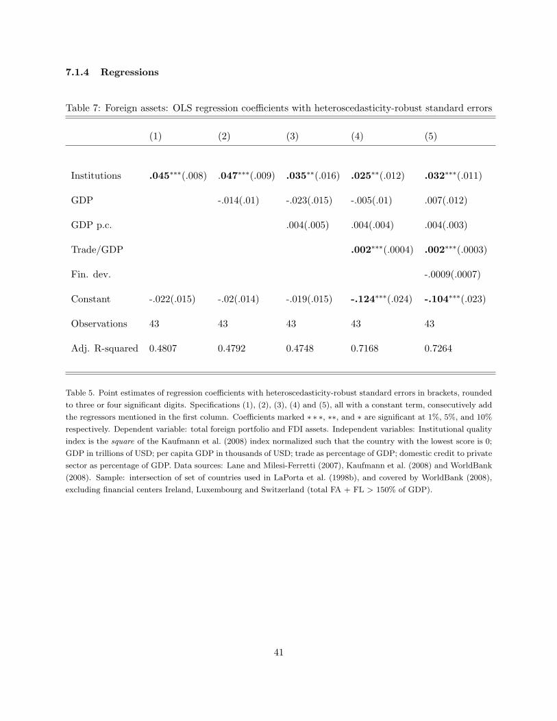
7.1.4 Regressions

Table 7: Foreign assets: OLS regression coefficients with heteroscedasticity-robust standard errors

(1) (2) (3) (4) (5)

Institutions .045∗∗∗(.008) .047∗∗∗(.009) .035∗∗(.016) .025∗∗(.012) .032∗∗∗(.011)

GDP -.014(.01) -.023(.015) -.005(.01) .007(.012)

GDP p.c. .004(.005) .004(.004) .004(.003)

Trade/GDP .002∗∗∗(.0004) .002∗∗∗(.0003)

Fin. dev. -.0009(.0007)

Constant -.022(.015) -.02(.014) -.019(.015) -.124∗∗∗(.024) -.104∗∗∗(.023)

Observations 43 43 43 43 43

Adj. R-squared 0.4807 0.4792 0.4748 0.7168 0.7264

Table 5. Point estimates of regression coefficients with heteroscedasticity-robust standard errors in brackets, rounded

to three or four significant digits. Specifications (1), (2), (3), (4) and (5), all with a constant term, consecutively add

the regressors mentioned in the first column. Coefficients marked ∗ ∗ ∗, ∗∗, and ∗ are significant at 1%, 5%, and 10%

respectively. Dependent variable: total foreign portfolio and FDI assets. Independent variables: Institutional quality

index is the square of the Kaufmann et al. (2008) index normalized such that the country with the lowest score is 0;

GDP in trillions of USD; per capita GDP in thousands of USD; trade as percentage of GDP; domestic credit to private

sector as percentage of GDP. Data sources: Lane and Milesi-Ferretti (2007), Kaufmann et al. (2008) and WorldBank

(2008). Sample: intersection of set of countries used in LaPorta et al. (1998b), and covered by WorldBank (2008),

excluding financial centers Ireland, Luxembourg and Switzerland (total FA + FL > 150% of GDP).

41

Table 8: Foreign liabilities: OLS regression coefficients with heteroscedasticity-robust standarderrors

(1) (2) (3) (4) (5)

Institutions .031∗∗∗(.007) .034∗∗∗(.008) .049∗∗∗(.011) .04∗∗∗(.008) .045∗∗∗(.008)

GDP -.023∗∗(.01) -.011(.012) .005(.008) .014(.009)

GDP p.c. -.005(.004) -.005∗∗(.002) -.006∗∗(.003)

Trade/GDP .002∗∗∗(.0002) .002∗∗∗(.0001)

Fin. dev. -.0006(.0003)

Constant .086∗∗∗(.019) .09∗∗∗(.018) .089∗∗∗(.018) -.006(.021) .008(.023)

Observations 43 43 43 43 43

Adj. R-squared 0.3528 0.3830 0.3912 0.6987 0.7026

Table 6. Point estimates of regression coefficients with heteroscedasticity-robust standard errors in brackets, rounded

to three or four significant digits. Specifications (1), (2), (3), (4) and (5), all with a constant term, consecutively

add the regressors mentioned in the first column. Coefficients marked ∗ ∗ ∗, ∗∗, and ∗ are significant at 1%, 5%, and

10% respectively. Dependent variable: total foreign portfolio and FDI liabilities. Independent variables: Institutional

quality index is the square of the Kaufmann et al. (2008) index normalized such that the country with the lowest score

is 0; GDP in trillions of USD; per capita GDP in thousands of USD; trade as percentage of GDP; domestic credit

to private sector as percentage of GDP. Data sources: Lane and Milesi-Ferretti (2007), Kaufmann et al. (2008) and

WorldBank (2008). Sample: intersection of set of countries used in LaPorta et al. (1998b), and covered by WorldBank

(2008), excluding financial centers Ireland, Luxembourg and Switzerland (total FA + FL > 150% of GDP).

42

7.2 Appendix B

7.2.1 Planner’s problem

The social planner allocates consumption between outsiders of the two countries taking the sum of income (labor

and dividend income) in each period as given (denoted by subscript “eq”). Since the planner has a static allocation

problem after the realization of the state st, I drop the state notation. Since asset trade takes place between outsiders

only, any capital gains do not affect the sum of their incomes.

max{C,C∗}

U(C,Leq) + U(C∗, L∗eq)

subject to,

C(st) + eeqC∗ = ψ0qaeqYaeq + ψ∗0qbeqYbeq + (1− α)Deq + (1− α)eeqD

∗eq

The solution to this problems requiresUCUC∗

=1

e

Portfolios which yield this allocation of consumption between outsiders will effectively replicate the constrained Pareto

efficient allocation in this economy.

7.2.2 Proof of Proposition 1

Consider the budget constraints of the outsiders in the two countries.

C(st) + P (st)(λNN (st)− λNN (st−1)) + e(st)P ∗(st)(λNS(st)− λNS(st−1))

= qa(st)W (st)L(st) + λNN (st)D(st) + λNS(st)e(st)D∗(st)

C∗(st) +P (st)(λSN (st)− λSN (st−1))

e(st)+ P ∗(st)(λSS(st)− λSS(st−1))

= qa(st)W (st)L(st) +λSN (st)D(st)

e(st)+ λSS(st)D∗(st)

With time invariant optimal portfolio shares the budget constraints reduce to

C(st) = qa(st)W (st)L(st) + λNND(st) + λNSe(st)D∗(st)

C∗(st) = qb(st)W ∗(st)L∗(st) +

λSND(st)

e(st)+ λSSD

∗(st)

Using the first order conditions for employment and stealing from the insiders’ problem,

W (st)L(st) =1− θα

(α+

(1− α)2

2η

)Ya(st)

W ∗(st)L∗(st) =1− θα

(α+

(1− α)2

2η

)Yb(s

t)

f(st) =1− αη

f∗(st) =1− αη

the dividend flows

43

D(st) = qa(st)[{1− f(st)}{Ya(st)} −W (st)L(st)]− {K(st)− (1− δ)K(st−1)}

D∗(st) = qb(st)[{1− f∗(st)}{Yb(st)} −W ∗(st)L∗(st)]− {K∗(st)− (1− δ)K∗(st−1)}

can be written as

D(st) = qa(st)Ya(st)[ψ1 − ψ0]− I(st)

D∗(st) = qb(st)Yb(s

t)[[ψ1 − ψ0]]− I∗(st)

where

ψ0 = (1− θ){1 +(1− α)2

2αη}

ψ1 =η + α− 1

η

Thus the budget constraints reduce to

C(st) = ψ0y(st) + λNN [(ψ1 − ψ0)y(st)− I(st)] + λNSe(st)[(ψ1 − ψ0)y∗(st)− I∗(st)]

C∗(st) = ψ0y∗(st) +

λSNe(st)

[(ψ1 − ψ0)y(st)− I(st)] + λSS [(ψ1 − ψ0)y∗(st)− I∗(st)]

where, for notational simplicity, I have

I(st) = K(st)− (1− δ)K(st−1)

I∗(st) = K∗(st)− (1− δ)K∗(st−1)

y(st) = qa(st)Ya(st)

y∗(st) = qb(st)Yb(s

t)

With logarithmic utility, the planner’s constrained Pareto efficient consumption allocations are

C(st) = e(st)C∗(st)

If there exists a portfolio share λ such that this condition holds for all states, then λ must satisfy

C(st)− e(st)C∗(st) = [ψ0 + (ψ1 − ψ0)(2λ+ α− 1)]{y(st)− e(st)y∗(st)} − (2λ+ α− 1){I(st)− e(st)I∗(st)} = 0

where I have expressed all portfolio shares in terms of λ by using symmetry and market clearing in asset markets,

which imply

λNN = λ

λSN = 1− α− λ

λNS = 1− α− λ

λSS = λ

44

Now,

y(st) = qa(st)Ya(st)

= qa(st){a(st) + a∗(st)}

= ωY (st) + (1− ω)e(st)Y ∗(st)

and

y∗(st) = qb(st)Yb(s

t)

= qb(st){b(st) + b∗(st)}

= (1− ω)Y (st)

e(st)+ ωY ∗(st)}

Henceforth for all variables x, ∆x(st) denotes the value of x(st)− e(st)x∗(st). Therefore

∆y(st) = y(st)− e(st)y∗(st)

= (2ω − 1){Y (st)− e(st)Y ∗(st)}

= (2ω − 1)∆Y (st)

Using the final-goods market-clearing conditions and the expression for the insiders’ consumption demand

Y (st) = C(st) +K(st)− (1− δ)K(st−1) +M(st) + Φ(st)

Y ∗(st) = Cm∗(st) +K∗(st)− (1− δ)K∗(st−1) +M∗(st) + Φ∗(st)

M(st) = αD(st) + qa(st)f(st)Ya(st)− Φ(st)

M∗(st) = αD∗(st) + qb(st)f∗(st)Yb(s

t)− Φ∗(st)

together with the expressions for the optimal stealing fraction and dividends, we have

∆y(st) = (2ω − 1)∆Y (st)

= (2ω − 1)[∆C(st) + ∆I(st) + {αθ +(1 + θ)(1− α)2

2η}∆y(st)− α∆I(st)

This gives after some algebra

∆y(st) =(2ω − 1)

ψ2{∆C(st) + (1− α)∆I(st)}

where

ψ2 = 1− (2ω − 1){αθ +(1 + θ)(1− α)2

2η}

Now, plugging in the value of ∆y(st) in the expression for ∆C(st), we get, for some constant µ

µ∆C(st) = [ψ2−1(1− α)(2ω − 1){ψ0 + (ψ1 − ψ0)(2λ+ α− 1)} − (2λ+ α− 1)]∆I(st)

This expression gives us the value of the portfolio share, λ, that will ensure that the complete markets condition,

∆C(st) = 0, holds for all states. The value of λ is calculated by simply assuming this the condition holds, and then

45

solving for λ.

This completes the proof of Proposition 1 in section (4.2).

7.2.3 Proof of Proposition 2

Since portfolio shares are constant, consumption of Northern and Southern outsiders can be written as,

C(st) = qa(st)W (st)L(st) + λNND(st) + λNSe(st)D∗(st)

C∗(st) = qb(st)W ∗(st)L∗(st) +

λSND(st)

e(st)+ λSSD

∗(st)

Denote qa(st)W (st)L(st) by L and qb(st)W ∗(st)L∗(st) by L∗. λ ensures that

C(st) = e(st)C∗(st)

Plugging in the values for consumption and log-linearizing the above relationship around the symmetric steady-state

we get,

LL + DDλ+ eD∗D∗(1− α− λ) + eD∗e(1− α− λ) = eL∗L∗ + eL∗e+ DD(1− α− λ) + eD∗D∗λ+ eD∗eλ

Gathering terms and noting that D∗ = D, L∗ = L, e = 1 in a symmetric equilibrium we get

(2λ+ α− 1)D(D − e− D∗) = L(L− e− L∗)

Denoting (D − e− D∗) as ∆D and (L− e− L∗) as ∆L we get

(2λ+ α− 1)D∆D = L∆L

which gives,

(2λ+ α− 1) = − LD

cov(∆L,∆D)

var(∆D)

Solving for λ gives the result.

7.3 Appendix C

7.3.1 The steady-state with symmetric countries (and Cobb-Douglas)

If the countries are ex-ante symmetric, then {qssa , q∗ssa , qssb , q∗ssb } simply reduce to

qssa = ωω(1− ω)1−ω (7.1)

q∗ssa = ωω(1− ω)1−ω (7.2)

qssb = ωω(1− ω)1−ω (7.3)

q∗ssb = ωω(1− ω)1−ω (7.4)

46

and Lss = L∗ss, ψ0 = ψ∗0 , ψ1 = ψ∗1. Thus the non-stochastic steady-state values of all other variables can be

expressed in terms of just Lss when the countries are symmetric. The quantity variables are

Kss =[ θ

1− θψ0q

ssa

1β

+ δ − 1

] 11−θ

Lss (7.5)

K∗ss =[ θ

1− θψ∗0q

∗ssb

1β

+ δ − 1

] 11−θ

L∗ss (7.6)

Y ssa =[ θ

1− θψ0ω

ω(1− ω)1−ω

1β

+ δ − 1

] θ1−θ

Lss (7.7)

Y ssb =[ θ

1− θψ0ω

ω(1− ω)1−ω

1β

+ δ − 1

] θ1−θ

Lss (7.8)

ass = ωY ssa = ω[ θ

1− θψ0ω

ω(1− ω)1−ω

1β

+ δ − 1

] θ1−θ

Lss (7.9)

a∗ss = (1− ω)Y ssa = (1− ω)[ θ

1− θψ0ω

ω(1− ω)1−ω

1β

+ δ − 1

] θ1−θ

Lss (7.10)

bss = (1− ω)Y ssa = (1− ω)[ θ

1− θψ0ω

ω(1− ω)1−ω

1β

+ δ − 1

] θ1−θ

Lss (7.11)

b∗ss = ωY ssa = ω[ θ

1− θψ0ω

ω(1− ω)1−ω

1β

+ δ − 1

] θ1−θ

Lss (7.12)

Y ss = qssa Yssa = ωω(1− ω)1−ω

[ θ

1− θψ0ω

ω(1− ω)1−ω

1β

+ δ − 1

] θ1−θ

Lss (7.13)

Y ∗ss = q∗ssb Y ssb = ωω(1− ω)1−ω[ θ

1− θψ0ω

ω(1− ω)1−ω

1β

+ δ − 1

] θ1−θ

Lss (7.14)

Dss =[ (1− θ)

θ

(ψ1 − ψ0)

ψ0(

1

β+ δ − 1)− δ

]Kss (7.15)

D∗ss =[ (1− θ)

θ

(ψ1 − ψ0)

ψ0(

1

β+ δ − 1)− δ

]Kss (7.16)

Css = (1− α)Dss + qssa WssLss (7.17)

C∗ss = (1− α)D∗ss + q∗ssb W ∗ssL∗ss (7.18)

Mss = α(1

β− 1)Kss (7.19)

M∗ss = α∗(1

β− 1)K∗ss (7.20)

Iss = δKss = δ[ θ

1− θψ0q

ssa

1β

+ δ − 1

] 11−θ

Lss (7.21)

I∗ss = δK∗ss = δ[ θ

1− θψ∗0q

∗ssb

1β

+ δ − 1

] 11−θ

L∗ss (7.22)

The parameters η and η∗ are selected such that steady state dividends are positive. In particular

η >(1− α){θ(1− α)(1− 1

β)− (2− α)( 1

β+ δ − 1)}

(1− 2α)( 1β

+ δ − 1) + 2αθ( 1β− 1)

47

fss =1− αη

(7.23)

f∗ss =1− α∗

η∗(7.24)

and the other prices are

P ss =β

1− βDss (7.25)

P ∗ss =β

1− βD∗ss (7.26)

Rss =1

β− 1 (7.27)

R∗ss =1

β− 1 (7.28)

W ss = ψ0Kss

Lss

θ

(7.29)

W ∗ss = ψ∗0K∗ss

L∗ss

θ

(7.30)

ess = 1 (7.31)

As in other models with portfolio selection like Devereux and Sutherland (2007) and Heathcote and Perri (2009),

the value of portfolios in the non-stochastic steady-state is indeterminate. With ex-ante symmetric countries, any

symmetric value of {λNN , λSS} is an equilibrium, so that

λNN = λSS ∈ [0, 1] (7.32)

λSN = 1− α− λNN (7.33)

λNS = 1− α∗ − λSS (7.34)

As a reminder

ψ0 = (1− θ){1 +(1− α)2

2αη}

ψ1 =η + α− 1

η

7.3.2 The steady-state with asymmetric countries

The steady-state value of {Kss,K∗ss} can be expressed in terms of {qssa , q∗ssa , qssb , q∗ssb }, and {Lss, L∗ss}, the

latter pair being calibrated to the data.

Kss =[ θ

1− θψ0q

ssa

1β

+ δ − 1

] 11−θ

Lss (7.35)

K∗ss =[ θ

1− θψ∗0q

∗ssb

1β

+ δ − 1

] 11−θ

L∗ss (7.36)

Substituting in the production function for intermediate goods we get

48

Y ssa = KssθLss1−θ =[ θ

1− θψ0q

ssa

1β

+ δ − 1

] θ1−θ

Lss (7.37)

Y ssb = K∗ssθL∗ss

1−θ=[ θ

1− θψ∗0q

∗ssb

1β

+ δ − 1

] θ1−θ

L∗ss (7.38)

(7.39)

and from the definition of dividends, the budget constraints of the four agents, and the final goods resource constraint

we have

Dss =[ (1− θ)

θ

(ψ1 − ψ0)

ψ0(

1

β+ δ − 1)− δ

]Kss (7.40)

D∗ss =[ (1− θ)

θ

(ψ∗1 − ψ∗0)

ψ∗0(

1

β+ δ − 1)− δ

]K∗ss (7.41)

Css = Y ss −Mss − Iss − Φss (7.42)

C∗ss = Y ∗ss −M∗ss − I∗ss − Φ∗ss (7.43)

Mss = α(1

β− 1)Kss (7.44)

M∗ss = α∗(1

β− 1)K∗ss (7.45)

(7.46)

and the other prices are

P ss =β

1− βDss (7.47)

P ∗ss =β

1− βD∗ss (7.48)

Rss =1

β− 1 (7.49)

R∗ss =1

β− 1 (7.50)

W ss = ψ0Kss

Lss

θ

(7.51)

W ∗ss = ψ∗0K∗ss

L∗ss

θ

(7.52)

(7.53)

The trade balance is zero in the steady-state. Using this fact, and the first order conditions for combining intermediate

goods, we get

49

ass =ωρ

ωρ + (1− ω)ρY ssa (7.54)

a∗ss =(1− ω)ρ

ωρ + (1− ω)ρY ssa (7.55)

bss =(1− ω)ρ

ωρ + (1− ω)ρY ssb (7.56)

b∗ss =ωρ

ωρ + (1− ω)ρY ssb (7.57)

With ρ = 1 (Cobb-Douglas) we have

qssa = ωω(1− ω)1−ω(K∗K

)θ(1−ω)

(7.58)

q∗ssa = ωω(1− ω)1−ω(K∗K

)θω(7.59)

qssb = ωω(1− ω)1−ω( KK∗

)θω(7.60)

q∗ssb = ωω(1− ω)1−ω( KK∗

)θ(1−ω)

(7.61)

ess =(K∗K

)θ(1−2ω)

(7.62)

tss =(K∗K

)θ(7.63)

where t is the terms of trade of the North, all in terms of K and K∗. Using the expression connecting K and K∗

to qa and q∗b , and the first order conditions for intermediate goods usage we get the expression for the steady-state

capital stock as

Kss = ζζ1

ζ21−ζ2

2 ζ∗ζ2

ζ21−ζ2

2 (7.64)

K∗ss = ζζ2

ζ21−ζ2

2 ζ∗ζ1

ζ21−ζ2

2 (7.65)

where

ζ =[ θ

1− θψ0ω

ω(1− ω)1−ω

1β

+ δ − 1

] 11−θ

Lss (7.66)

ζ∗ =[ θ

1− θψ∗0ω

ω(1− ω)1−ω

1β

+ δ − 1

] 11−θ

L∗ss (7.67)

ζ1 =1− θω1− θ (7.68)

ζ2 =θ(1− ω)

1− θ (7.69)

Note that we can get symmetric countries as a special case of the above, when ζ = ζ∗. For the general aggregating

function, we have, following the same procedure

50

qssa =[ωρ + (1− ω)ρ

(K∗K

) θ(ρ−1)ρ] 1

ρ−1(7.70)

q∗ssa =[(1− ω)ρ + ωρ

(K∗K

) θ(ρ−1)ρ] 1

ρ−1(7.71)

qssb =[ωρ( KK∗

) θ(ρ−1)ρ

+ (1− ω)ρ] 1

ρ−1(7.72)

q∗ssb =[(1− ω)ρ

( KK∗

) θ(ρ−1)ρ

+ ωρ] 1

ρ−1(7.73)

ess =[ωρK θ(ρ−1)

ρ + (1− ω)ρK∗θ(ρ−1)

ρ

(1− ω)ρKθ(ρ−1)

ρ + ωρK∗θ(ρ−1)

ρ

] 1ρ−1

(7.74)

tss =( ω

1− ω

)1−ρ(K∗K

)θ(7.75)

and capital stocks are solved from the simultaneous equations

Kss =[ θ

1− θ

ψ0

[ωρ + (1− ω)ρ

(K∗

K

) θ(ρ−1)ρ] 1

ρ−1

1β

+ δ − 1

] 11−θ

Lss (7.76)

K∗ss =[ θ

1− θ

ψ∗0

[(1− ω)ρ

(KK∗

) θ(ρ−1)ρ

+ ωρ] 1

ρ−1

1β

+ δ − 1

] 11−θ

L∗ss (7.77)

7.4 Appendix D

This section contains descriptions of the numerical algorithms used in the paper.

7.4.1 Algorithm for computing approximate equilibrium for outsiders

1. The first step is to find a point around which to approximate the decision rules. This point is the unique stationary

solution to the set of equilibrium conditions of the model, for the case when there is no uncertainty, that is, the scale

parameter of the variance of the driving shocks is equal to zero. This is called the non-stochastic steady-state. To

ensure stationarity of all variables, and a zero-current account, I follow Schmitt-Grohe and Uribe (2003) in positing

a convex portfolio adjustment cost, which pins down a unique non-stochastic steady-state for portfolio variables,

and hence for financial wealth. The approximation point for portfolio shares, (λNN , λNS), (λSN , λSS) is arbitrary

at this juncture, because in the non-stochastic steady-state, any portfolio share which keeps the wealth distribution

unchanged with respect to the initial endowment of shares, is an equilibrium. We assume a small convex adjustment

cost of changing portfolios from (λNN , λNS), (λSN , λSS). This is done to keep the foreign wealth position of each

country stationary. As noted by Schmitt-Grohe and Uribe (2003), this modification does not significantly affect

the dynamics of other macroeconomic variables at the level of approximation that these models are analyzed. This

technique is also used by Heathcote and Perri (2009), and like them I find that the cost of adjustment τ , can be set

to an arbitrarily small positive number. Of course, the higher τ is set, the less portfolio shares will diverge from the

chosen value of (λNN , λNS), (λSN , λSS). In this model, I set τ to be 0.00001% of the un-weighted average steady-state

stock price. Thus the budget constraint of the outsider in the North is as follows.

51

C(st) + P (st)(λNN (st)− λNN ) + e(st)P ∗(st)(λNS(st)− λNS) +τ

2(λNN (st)− λNN )2

+τ

2(λNS(st)− λNS)2 = qa(st)W (st)L(st) + λNN (st−1)D(st) + λNS(st−1)e(st)D∗(st)

(7.78)

The steady-state values of all variables are provided in the previous section.

2. Around the chosen stationary steady-state, I find second-order Taylor series approximation of the optimal dynamics

of the control and state variables using the algorithm developed by Schmitt-Grohe and Uribe (2004).

7.4.2 Second-order optimal dynamics

This section provides a brief review of the approximation technique described in Schmitt-Grohe and Uribe (2004),

henceforth referred to as SGU, which is used to solve the model.24 The n equations characterizing the stochastic

equilibrium of this economy can be written in the form

Etf(yt+1, yt, xt+1, xt) = 0, f : <ny×ny×nx×nx → <n

y is a ny × 1 vector of control variables and x = (x1, x2)′

is a nx × 1 vector of state variables, where x1 and x2

are respectively (nx − nε) × 1 and nε × 1 vectors of endogenous and exogenous state variables. The non-stochastic

steady-state values of the arguments of f(.) are denoted by the set {yss, xss}, and these values can be solved from

f(yss, yss, xss, xss) = 0

Lemma 1 For the dynamic system described in the previous sections, there exists a unique, interior stationary

solution for all non-portfolio variables, denoted by {yss, xss}(−λ).

Proof: See previous section for steady state values. (7.3)

Following the notation of SGU, the solution to the model can be written in the form of two functions, g(x, σ)

which is the optimal policy function, and h(x, σ) which describes the transition of both the endogenous and exogenous

states. Thus

y = g(x, σ)

x′

= h(x, σ) + ησε′

where η is a nx × nε matrix, partly zeros, describing the variance-covariance structure of the errors in the exogenous

driving variables, which in this case are technology in the Northern and Southern intermediate goods sector. The two

functions g(x, σ) and h(x, σ) are approximated up to the second order by writing them as functions of the first and

second derivative of the function f in the neighborhood of the approximation point {yss, xss}. By solving a system

of linear equations whose co-efficient matrix comprises of these numerical derivatives of the known function f , the

SGU algorithm arrives at the functions g(x, σ) and h(x, σ). The row of the approximated policy function g(x, σ)

that is of paramount interest to us is the one which specifies stochastic-equilibrium portfolio allocations, λ(x, σ), as

24In general, though the certainty-equivalent non-stochastic steady-state, and first-order approximate solution ofthe model are the same, they do not coincide with the true stochastic solution. This is because second or higher orderterms of the true solution are significant in the presence of uncertainty. See Kim and Kim (2003) and Schmitt-Groheand Uribe (2004) for further discussions of this point.

52

a function of the state variables, and uncertainty. Further details of this method can be found in Schmitt-Grohe and

Uribe (2004).25

7.4.3 Algorithm for choosing portfolio approximation point

We search in the neighborhood of a set of points (λNN , λSS) ⊂ [0, 1] × [0, 1] for the “correct” (in a sense that

will be defined below) portfolio approximation point. We search among those points that keep (non-stochastic)

steady-state wealth distribution constant, and the current account balanced.

Lemma 2 The following locus of portfolios keeps (non-stochastic) steady-state wealth distribution constant, and the

current account balanced.

λNNPss − λSSP ∗ssess = (1− α)P ss − (1− α∗)P ∗ssess

Proof: Recall that the non-stochastic steady-state values of all variables except portfolio shares are determinate.

Also they are independent of the value of the portfolio shares, for example, labor incomes in any steady-state are

independent of λNN and λNS . Thus in any two non-stochastic steady-states (λNN , λNS) ∈ [0, 1]× [0, 1], denoted by

1 and 2, we must have

λhh1Dss + λhf1D

∗ssess = λhh2Dss + λhf2D

∗ssess

In particular

λNNDss + λNSD

∗ssess = (1− α)Dss

Using the stock market clearing condition in the North, and the expression for steady-state stock prices, this reduces

to the condition in the statement of the lemma. Also note that using the stock market clearing conditions in each

country, and the expression for stock steady-state stock prices

λNNPss − λSSP ∗ssess = (1− α)P ss − (1− α∗)P ∗ssess (7.79)

⇒ λSNPss = λNSP

∗ssess (7.80)

which implies that net steady-state transfers are zero. This means the current account is balanced.

7.4.4 Algorithm for insider’s choice of ownership

We are seeking a maximum of the function that maps insider ownership to expected lifetime utility of the insider.

1. Start with an initial distribution of ownership, α∗′.

2. Use the “golden search” algorithm. Choose an interval for α, say [αmin, αmax].

3. Approximate optimal decision rules of economy around steady-state with ownership αmin and αmax. Home

stock ownership of the Southern insider given by the budget constraint αSN = (α∗′−α∗)P0(α∗)P0(α)

for each scenario.

4. Simulate economy with above decision rules around αmin and αmax. Calculate average utility of insider in

simulations. Update interval according to “golden search” algorithm.

5. Repeat till convergence occurs.

25A possible issue with this approximation technique is that it ignores the possible heteroscedasticity in the en-dogenous variables (see Evans and Hnatkovska (2007) for a discussion). In the context of this model, this is lessof a problem because the feedback mechanism from asset returns, which depend on higher order moments of statevariables, to the decisions of the firms is weak because of the insider-outsider dichotomy.

53

7.5 Appendix E

7.5.1 Calibration and variables

Table 9:

Notation Explanation

Goodsa North intermediate good used in Northb South intermediate good used in Northa∗ North intermediate good used in Southb∗ South intermediate good used in SouthYa Total North intermediate good producedYb Total South intermediate good produced

Price of goods and servicesqa North intermediate good price in Northqb South intermediate good price in Northq∗a North intermediate good price in Southq∗b South intermediate good price in South

W,W ∗ North, South wagese Real exchange ratet Terms of trade

Asset market quantities and pricesP, P ∗ North, South stock pricesα, α∗ Insider ownership in the North, SouthλNN North outsider’s ownership of Northern assetλSN South outsider’s ownership of Northern assetλNS North outsider’s ownership of Southern assetλSS South outsider’s ownership of Southern asset

Parametersβ = 0.99 Discount factorθ = 0.34 Capital shareδ = 0.025 Depreciationω = 0.15 Import share

Z(t) = 0.91Z(t− 1) + ε(t) Domestic shocksZ∗(t) = 0.91Z∗(t− 1) + ε∗(t) Foreign shocks

σ2ε = 0.0062 Variance of technology shocks

54