coulomb excitation of 200po studied at rex-isolde with the

FACULTEIT WETENSCHAPPENDepartement Natuurkunde en SterrenkundeInstituut voor Kern- en Stralingsfysica

Coulomb excitation of 200Po studied at REX-ISOLDEwith the Miniball γ spectrometer

door

Nele KESTELOOT

Promotor: Prof. dr. P. Van Duppen Proefschrift ingediend tot hetbehalen van de graad vanMaster in de Fysica

Academiejaar 2009-2010

Dankwoord

Alvorens van start te gaan met het “echte” werk, wil ik graag alle mensen bedanken dieop een of andere manier hebben bijgedragen tot de thesis die nu voor u ligt. In de eersteplaats richt ik mij tot mijn promotor Piet Van Duppen en Mark Huyse. Bedankt voorhet ongelofelijk boeiende en aangename jaar dat ik mocht spenderen in de groep.

Dat jaar was zeker niet hetzelfde geweest moest ik op een andere bureau terecht zijngekomen. In de tweede plaats bedank ik dan ook graag mijn begeleider Nick. Nick, ik hebontzettend veel van je geleerd dit jaar. Ik apprecieer het enorm dat je altijd uitgebreidde tijd nam om je “over mij te ontfermen”. Voor de aangename sfeer op de bureau wil ikook Jan bedanken. Nick en Jan, door jullie zag ik er (bijna) nooit tegen op om aan mijnthesis te komen werken, jullie zorgden ervoor dat er veel meer dan alleen maar kernfysicate beleven viel. Ondanks de veelvuldige “seeeg” vind ik het leuk dat jullie zo goed voorme gezorgd hebben: van de registratie-doolhof in CERN over de vele programmeer-, enfysicavraagjes tot de gezellige rookpauzes. Bedankt!

Of course I also want to thank Beyhan for introducing me to the fascinating world ofpolonium nuclei and for the discussions about the analysis that we performed in parallel.Another big thank you goes to Iain for your ever-honest opinion on things, especially forhelping me with the presentation. Er is natuurlijk ook leven buiten onze bureau. Daaromwil ik graag alle andere IKS-ers bedanken en dan vooral de kernspectroscopiegroep. Inhet bijzonder dank ik Jytte voor de vele babbeltjes wanneer ik het even beu was.

Deze thesis is de afronding van vijf jaren fysica. Daarom wil ik graag mijn medestu-denten bedanken en dan vooral Jan, Seb, Geert, Kelly, Bart en Sander. Bedankt voor degezellige middagpauzes, de late-night thesis momenten, alle lessen samen en vooral: dater nog veel gehaktfeestjes mogen volgen!

Hanne, bedankt om de beproeving te doorstaan en je door 70 bladzijden kernfysica teworstelen voor me! Verder wil ik graag al mijn vrienden bedanken waarbij ik mijn energiekwijt kon in vele ontspannende momenten: alle mensen van HONK!, mijn vriendinnenvan het thuisfront, de medebegeleiding van de Plussers en mijn voetbalploeg.

Mama, papa, Lore en Wouter: bedankt! Voor de steun, de interesse, de gezelligheiden vooral om me mijn enthousiaste en prettig gestoorde zelf te laten zijn thuis, zelfs alsik helemaal gek werd tijdens de blok.

Stijn, bedankt voor je onvoorwaardelijke steun, vertrouwen en liefde!

Samenvatting

De polonium isotopen bevinden zich in een zeer interessant gebied van de kernkaart ver-mits ze slechts twee protonen buiten de gesloten Z = 82 schil bezitten. Er is dan ook,zowel op theoretisch als op experimenteel vlak, al veel onderzoek gebeurd naar de ver-schillende polonium isotopen. Uit de resultaten van dat onderzoek blijkt dat 200Po eenovergangskern is. De zware polonium isotopen (met massagetal A > 200) volgen een “se-nioriteitsregime” terwijl er in de lichtste polonium isotopen (A < 198) zowel experimenteelals theoretisch bewijs is voor een coexistentie van verschillende vormen van de kern. Dewijze waarop de overgang tussen deze twee regimes gebeurt is nog niet goed gekend. Daar200Po zich in dit overgangsgebied bevindt, kan de studie van deze atoomkern ons iets lerenover het ontstaan van vormcoexistentie. Dit fenomeen waarbij de atoomkern twee of meerverschillende vormen kan aannemen is nog niet voldoende begrepen. Vooral de mengingtussen de twee kwantumtoestanden moet verder onderzocht worden. In dit werk wordtCoulomb excitatie gebruikt om 200Po te bestuderen.

Wanneer een projectiel met grote energie op een doelwit wordt geschoten, zullen zowelprojectiel als doelwit verstrooid worden. Wanneer tijdens de interactie tussen beide kernenhet virtueel foton van de elektromagnetische interactie wordt uitgewisseld, wordt een vande twee kernen geexciteerd. In dat geval wordt het verstrooiingsproces inelastisch genoemden spreekt men van Coulomb excitatie. Door Coulomb excitatie kunnen de geexciteerdetoestanden met kleine excitatie-energie bevolkt worden. De werkzame botsingsdoorsnedevoor Coulomb excitatie hangt in eerste orde af van de gereduceerde overgangswaarschi-jnlijkheid B(E2, Ii → If ). In tweede orde hangt de botsingsdoorsnede ook af van hetquadrupoolmoment van de gepopuleerde toestanden. De B(E2, Ii → If ) waarde is eenmaat voor de collectiviteit van de kern en het quadrupoolmoment drukt de mate uitwaarin de vorm van de kern afwijkt van sferische symmetrie. Vermits deze twee observ-abelen kunnen bepaald worden met een Coulomb excitatie experiment, leent de techniekvan Coulomb excitatie zich uiterst goed om de overgangskern 200Po te onderzoeken. Dezethesis beschrijft de motivatie, de experimentele opstelling en de data-analyse van eenCoulomb excitatie experiment op 200Po.

Het Coulomb excitatie experiment vond plaats in REX-ISOLDE (CERN, Geneve,Zwitserland) waar een 200Po bundel werd geproduceerd en naversneld tot een energie van2.85 MeV/u. Deze bundel werd gericht op een 104Pd doelwit waarna nauwkeurig werdbestudeerd wat er gebeurde in de doelwitkamer. Om de verstrooide kernen te bestud-eren werd gebruik gemaakt van een positiegevoelige dubbelzijdige silicium strip detector.De gammastralen die worden uitgezonden bij de de-excitatie van de geexciteerde kernenworden gedetecteerd met de Miniball gamma spectrometer die eveneens positiegevoelig

i

ii

is. De positiegevoeligheid is vereist omdat de energie van de de-excitatie gammastralenDoppler verschoven wordt. De kernen vervallen immers voordat ze gestopt zijn in desilicium detector. Om te kunnen corrigeren voor deze Doppler verschuiving is de positievan de kern en van de gammastraal nodig. Voor de detectie van de gammastralen met deMiniball detector werd een absolute efficientiecurve afgeleid aan de hand van vervaldatavan 152Eu, 133Ba en 241Am.

Bij Coulomb excitatie moeten er steeds drie dingen gelijktijdig bestudeerd worden:twee verstrooide kernen in de siliciumdetector en een gammastraal in de MINIBALL de-tector. Een heel belangrijk deel in de analyse van het experiment bestaat er dus uit omdeze interessante gebeurtenissen te selecteren. Om dit correct te kunnen doen, moet dedeeltjesdetector gecalibreerd worden en moeten er voorwaarden worden opgelegd waaraande gammastralen moeten voldoen om verbonden te kunnen worden met een Coulombexcitatie gebeurtenis. Wanneer de interessante gebeurtenissen geselecteerd zijn, kan erworden gekeken naar het gammaspectrum. Dit spectrumn toonde een fotopiek waarvande energie in overeenstemming was met de energie van de bekende 2+

1 → 0+1 overgang

in 200Po en een zeer grote hoeveelheid polonium K-X stralen te zien. Op basis hiervanwerd besloten dat de 2+

1 en de 0+2 toestand in 200Po bevolkt werden tijdens het Coulomb

excitatie experiment. De 0+2 toestand vervalt immers via een E0 overgang naar de grond-

toestand. Deze E0 overgang gaat gepaard met het uitzenden van karakteristieke poloniumK-X stralen. De overgang van de 0+

2 toestand naar de 2+1 toestand werd niet geobserveerd.

Deze vaststelling komt overeen met het resultaat van een β+/elektronvangst studie van200Po waarin deze gamma overgang eveneens niet werd geobserveerd maar de E0 overgangdaarentegen wel [Bij98].

De experimentele informatie die uit het Coulomb excitatie experiment werd gehaaldwerd daarna ingevoerd in GOSIA, een computercode speciaal ontworpen voor de anal-yse van Coulomb excitatie experimenten. GOSIA voert een χ2 minimalisatie uit doorde experimentele informatie te vergelijken met berekende informatie. In dit minimal-isatieproces worden de matrixelementen, die de toestanden verbinden die in het Coulombexcitatie experiment gevoed werden, gevarieerd. Als resultaat van de minimalisatie wor-den de matrixelementen gegeven waarbij de χ2 minimaal is. Deze matrixelementen zijnrechtstreeks verbonden met de eerder vermelde B(E2, Ii → If ) waarde en het quadrupool-moment.

Wanneer alle beschikbare experimentele informatie in GOSIA werd ingegeven, wasGOSIA niet in staat om fysische resultaten te produceren. De onverwacht grote hoeveel-heid polonium K-X stralen en het niet observeren van de 0+

2 → 2+1 overgang maken de

minimalisatie blijkbaar zeer moeilijk. Als tijdelijk compromis werd een vereenvoudigdsysteem, dat enkel bestaat uit de grondtoestand en de 2+

1 toestand, ingevoerd in GOSIA.Uit dit systeem werd een B(E2, 0+

1 → 2+1 ) waarde van 29(4

6) W.u. gehaald en een diagonaalmatrixelement 〈2+

1 ||E2||2+1 〉 van 0.55(85

85) eb gehaald. De B(E2, 0+1 → 2+

1 ) werd vergelekenmet de bekende B(E2, 0+

1 → 2+1 ) waarden in andere poloniumisotopen.

Het spreekt voor zich dat de analyse van dit experiment gefinaliseerd moet wordendoor te zoeken naar een manier om de informatie over de 0+

2 toestand ook in acht tenemen in de GOSIA berekeningen. Op die manier kan een waarde bekomen worden voor

iii

het 〈2+1 ||E2||0+

2 〉 matrixelement en worden de afgeleide waarden voor het 〈0+1 ||E2||2+

1 〉en 〈2+

1 ||E2||2+1 〉 matrixelement ook beınvloed. Verder dient de Coulomb excitatie studie

uitgebreid te worden naar 196,198,202Po om de eerder besproken overgang helemaal in kaartte kunnen brengen. De bundeltijd voor deze experimenten wordt waarschijnlijk in 2011gepland.

Contents

Samenvatting . . . . . . . . . . . . . . . . . . . . . . . . . . . . . . . . . . . . . iContents . . . . . . . . . . . . . . . . . . . . . . . . . . . . . . . . . . . . . . . . iv

Introduction 1

1 Motivation 21.1 Nuclear structure . . . . . . . . . . . . . . . . . . . . . . . . . . . . . . . . 21.2 Nuclear models . . . . . . . . . . . . . . . . . . . . . . . . . . . . . . . . . 3

1.2.1 Shell model . . . . . . . . . . . . . . . . . . . . . . . . . . . . . . . 41.2.2 Deformed nuclei . . . . . . . . . . . . . . . . . . . . . . . . . . . . . 6

1.3 Experimental observables . . . . . . . . . . . . . . . . . . . . . . . . . . . . 81.4 Why 200Po? . . . . . . . . . . . . . . . . . . . . . . . . . . . . . . . . . . . 10

1.4.1 Experimental achievements in the polonium isotopes . . . . . . . . 101.4.2 Theoretical considerations . . . . . . . . . . . . . . . . . . . . . . . 12

1.5 Why Coulomb excitation? . . . . . . . . . . . . . . . . . . . . . . . . . . . 171.5.1 Kinematics . . . . . . . . . . . . . . . . . . . . . . . . . . . . . . . 181.5.2 Cross section of Coulomb excitation . . . . . . . . . . . . . . . . . . 191.5.3 Application to the experiment . . . . . . . . . . . . . . . . . . . . . 221.5.4 Computer codes for the calculation of cross sections . . . . . . . . . 23

2 Experimental Setup 242.1 Production of the 200Po isotopes . . . . . . . . . . . . . . . . . . . . . . . . 242.2 Post acceleration by REX-ISOLDE . . . . . . . . . . . . . . . . . . . . . . 252.3 Time structure . . . . . . . . . . . . . . . . . . . . . . . . . . . . . . . . . 262.4 The detection system . . . . . . . . . . . . . . . . . . . . . . . . . . . . . . 27

2.4.1 The Miniball γ-detector array . . . . . . . . . . . . . . . . . . . . . 282.4.2 Efficiency of the γ detection . . . . . . . . . . . . . . . . . . . . . . 292.4.3 Double-sided silicon-strip detector . . . . . . . . . . . . . . . . . . . 38

2.5 The 104Pd target . . . . . . . . . . . . . . . . . . . . . . . . . . . . . . . . 40

3 Data Analysis 433.1 Energy Calibration of the DSSSD . . . . . . . . . . . . . . . . . . . . . . . 43

3.1.1 Problem in strip 8 . . . . . . . . . . . . . . . . . . . . . . . . . . . 463.2 Two-particle events . . . . . . . . . . . . . . . . . . . . . . . . . . . . . . . 47

3.2.1 Peak at low energy . . . . . . . . . . . . . . . . . . . . . . . . . . . 493.3 Determination of prompt and random window . . . . . . . . . . . . . . . . 523.4 Analysis of the γ spectra . . . . . . . . . . . . . . . . . . . . . . . . . . . . 55

3.4.1 Doppler correction . . . . . . . . . . . . . . . . . . . . . . . . . . . 57

iv

CONTENTS v

3.4.2 Integrals of the de-excitation peaks . . . . . . . . . . . . . . . . . . 603.5 X rays . . . . . . . . . . . . . . . . . . . . . . . . . . . . . . . . . . . . . . 633.6 GOSIA analysis . . . . . . . . . . . . . . . . . . . . . . . . . . . . . . . . . 643.7 Discussion . . . . . . . . . . . . . . . . . . . . . . . . . . . . . . . . . . . . 66

Conclusion 67

Bibliography i

Introduction

This thesis describes the motivation, experimental setup and analysis of a Coulomb-excitation experiment on 200Po. The first chapter starts with a general introduction tonuclear structure and a short description of different theoretical nuclear models. Therelevant experimental observables in a Coulomb-excitation experiment are also described.The main part of the first chapter reviews the theoretical and experimental work of thepolonium isotopes (Z = 84). This part serves as a motivation to why 200Po in particularwas studied. The final part of the first chapter describes the Coulomb-excitation tech-nique.

The experimental setup at REX-ISOLDE (CERN) that was used for the experimentis described in Chapter 2. Firstly the production of the 2.85 MeV/u 200Po beam is ex-plained. In a Coulomb-excitation experiment both particles and gamma rays have to bedetected. Hence a special detection setup is required for this kind of experiments. Thissetup is described and special attention is paid to the extraction of an absolute efficiencycurve of the gamma detection.

Chapter 3 describes in detail the analysis of the experimental data and the problemsthat showed up during the analysis. In a first step the particle detector is calibrated.The main part of the analysis consists of selecting the interesting physical events out ofthe background and extracting the useful information from these physical events. Finallythe results are inserted in GOSIA which is a Coulomb-excitation analysis code. GOSIAtranslates the experimentally obtained results into physical observables that provide in-formation on the nuclear structure of the studied nucleus.

1

Chapter 1

Motivation

This first chapter starts with a general introduction to nuclear structure and a shortdescription of different theoretical nuclear models. Also two-state mixing is explainedbriefly and the relevant experimental parameters are discussed. At the end of this chapterof this chapter, the study of 200Po and the reasons for using the technique of Coulombexcitation are motivated.

1.1 Nuclear structure

Figure 1.1: The nuclear chart with the number of neutrons N on the horizontal axisand the number of protons Z on the vertical axis. The different colors represent thedifferent decay modes (blue: β− decay, red: β+ decay/electron capture, yellow: α decay,green: spontaneous fission). The nuclei depicted in grey have not yet been observedexperimentally [Bea01].

An atom consists of a nucleus surrounded by an electron cloud. Nuclear structurephysics deals with the structure of the nucleus, which is composed of positively chargedprotons and uncharged neutrons, while the electrons are in most cases discarded. The

2

1.2 Nuclear models 3

atomic number Z represents the number of protons and determines the chemical elementand thus the position of the atom in the Periodic Table of Elements. The number of neu-trons N in the nucleus of a certain element can vary. Two nuclei with the same numberof protons but with a different number of neutrons are called isotopes of that particularelement. The mass number A (= Z + N) expresses the total number of protons andneutrons, which are called nucleons. To denote a particular nucleus with A nucleons andZ protons, the notation AX is used, with X representing the name of the element. Allthe theoretically predicted nuclei are depicted on the nuclear chart (see Figure 1.1) as afunction of the number of protons Z and the number of neutrons N. The nuclei in greyhave not yet been observed experimentally.

To date more than 3600 nuclei are known and 284 of them are stable. The remain-ing nuclei are radioactive. The stability of a nucleus is determined by the interactionbetween two forces. The repulsive electromagnetic force between the protons drives thenucleus apart. However this can be overcome on the femtometre scale (10−15 m) by thestrong nuclear force, which holds the nucleons together, provided that there is a sufficientamount of neutrons. It is clear that the ratio of the number of neutrons to the number ofprotons N/Z will play an important role in the stability of the nucleus. Indeed, this ratiodetermines if the nuclear force is strong enough to keep the nucleons together despite theelectromagnetic repulsion. Besides the electromagnetic and the strong interaction, alsothe weak interaction is important as it is responsible for the beta decay of nuclei. Thestable nuclei (indicated in black on Figure 1.1) are said to lie on the “beta stability line”.For low masses this line follows the N = Z trend, for higher masses it departs from theN = Z line towards the more neutron-rich nuclei. Nuclei with an extreme N/Z ratio arecalled “exotic”.

In order to understand the behavior of the different nuclei it is essential to describe indetail the nuclear medium, consisting of a finite number of interacting nucleons. Thereforethe Schrodinger equation HΨ(1, ...,A) =EΨ(1, ...,A) must be solved. The non-relativisticHamiltonian is given by:

H =A∑i=1

Ti +1

2

A∑i,j=1

Vi,j (1.1)

with A, Ti and Vi,j representing respectively the number of nucleons, the kinetic energy ofthe ith nucleon and the two-body interaction [Cas00]. Higher-order terms (e.g. three-bodyinteractions) are neglected here. This complex many-body problem can only be solvedanalytically for the lightest nuclei and the exact form of the two-body interaction is stillpoorly known. In order to describe the heavier nuclei a reasonable approximation is thusessential.

1.2 Nuclear models

Throughout the years different theoretical descriptions of the nucleus that simplify thecomplex many-body problem in their own way have been developed. A first step in thesimplification is to introduce a mean field and hereby splitting the Hamiltonian of equation


1.1 up in two parts

H =[ A∑i=1

(Ti + U(ri))]

+[1

2

A∑i,j=1

Vi,j −A∑i=1

U(ri)]

= H0 + H1 (1.2)

where U(ri) is a central mean-field potential generated by the nucleons themselves [Hey90].H0 is a sum of one-body Hamiltonians and describes the nucleons as independent particlesmoving in an average field. H1 represents the residual interaction between the particlesand can be treated as a perturbation when U(ri) is chosen appropriately. This mean-fieldpotential U(ri) can be determined empirically or in a self-consistent way (Hartree-Fockmethod). In the Hartree-Fock method one starts from a known nucleon-nucleon inter-action potential from which the mean-field potential is derived iteratively by demandingthat the Hartree-Fock energy is minimal. The harmonic-oscillator potential is an exampleof an empirical mean field and is used as a starting point in the shell model. This willbe explained more thoroughly in section 1.2.1. The mean-field approximation is validwhen the long-ranged components of the nucleon-nucleon interaction dominate. Howeverin general the short-ranged components (the interaction between the nucleons e.g. thepairing force) cannot simply be neglected. They can be incorporated after the calculationof the mean-field potential as in the Hartree-Fock + Bardeen-Cooper-Schrieffer method(HF + BCS) or they can be included in the process of determining the mean field as inthe Hartree-Fock-Bogolyubov (HFB) theory [Hey90].

1.2.1 Shell model

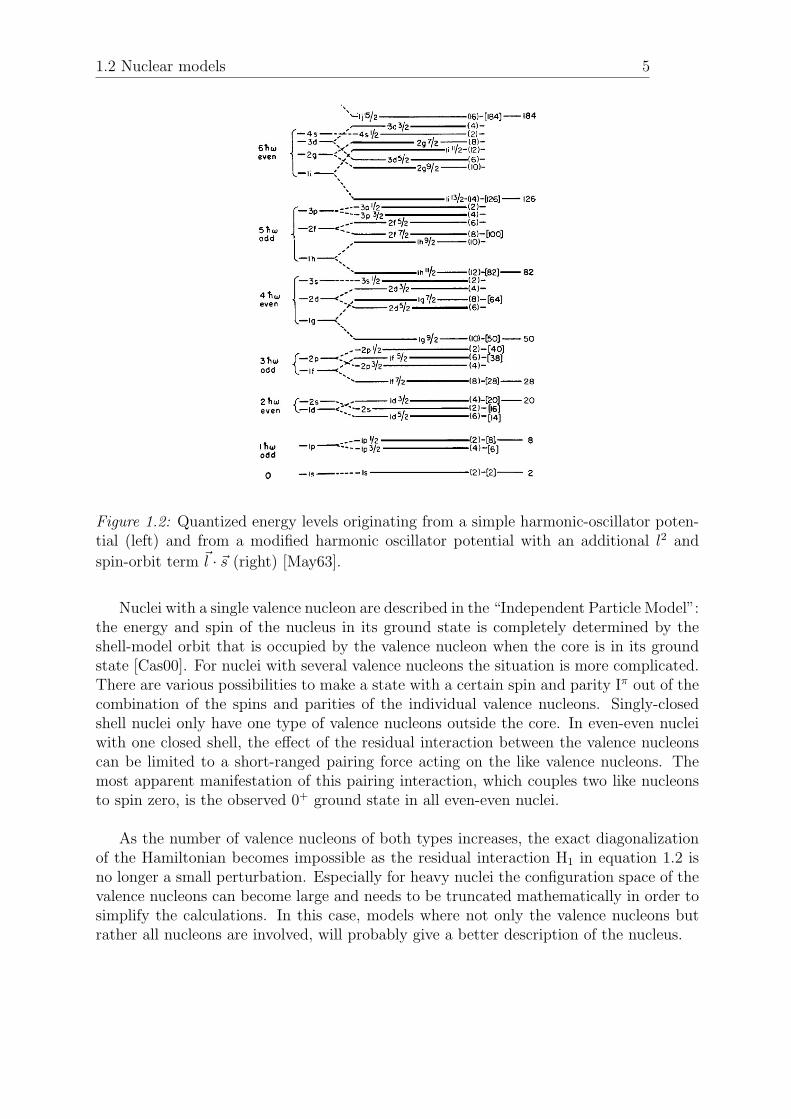
Experimental evidence points to a structure in nuclei that is comparable to the atomicshell structure. Certain numbers of protons and neutrons give rise to exceptionally stablenuclei. This stability is explained by the fact that this particular amount of protons orneutrons leads to the filling of a “shell” of energy levels. Near stability the so-called“magic”numbers are situated at N, Z = 2, 8, 20, 28, 50, 82, 126, ... The single-particleenergy levels group into “shells” that are separated by larger energy gaps, corresponding toa closed shell as illustrated in Figure 1.2. The quantized energy levels are solutions of theSchrodinger equation with the one-body Hamiltonian H0 (equation 1.2). When a simpleharmonic-oscillator potential is used as mean-field potential the observed magic numberscannot be reproduced. The mean field that reproduces the correct magic numbers is amodified harmonic-oscillator potential to which an attractive term in l2 and a spin-orbitterm ~l · ~s are added.

When omitting the residual interaction between the nucleons only doubly-magic nuclei(with a closed proton and neutron shell) can be described. These nuclei can be consideredas inert cores of non-interacting particles. The residual interaction is incorporated in aspecific way in the shell model. The observed shell structure of nuclei with large energygaps at closed shells justifies a separation of the nucleus into an inert core of inactive nu-cleons and a set of active (valence) nucleons outside this core. The valence nucleons movein a selected set of shell-model orbits and interact with each other through the residualinteraction. An appropriate choice of the configuration space (i.e. the orbits in which thenucleons are allowed to move) for the valence nucleons is essential.


Figure 1.2: Quantized energy levels originating from a simple harmonic-oscillator poten-tial (left) and from a modified harmonic oscillator potential with an additional l2 and

spin-orbit term ~l · ~s (right) [May63].

Nuclei with a single valence nucleon are described in the “Independent Particle Model”:the energy and spin of the nucleus in its ground state is completely determined by theshell-model orbit that is occupied by the valence nucleon when the core is in its groundstate [Cas00]. For nuclei with several valence nucleons the situation is more complicated.There are various possibilities to make a state with a certain spin and parity Iπ out of thecombination of the spins and parities of the individual valence nucleons. Singly-closedshell nuclei only have one type of valence nucleons outside the core. In even-even nucleiwith one closed shell, the effect of the residual interaction between the valence nucleonscan be limited to a short-ranged pairing force acting on the like valence nucleons. Themost apparent manifestation of this pairing interaction, which couples two like nucleonsto spin zero, is the observed 0+ ground state in all even-even nuclei.

As the number of valence nucleons of both types increases, the exact diagonalizationof the Hamiltonian becomes impossible as the residual interaction H1 in equation 1.2 isno longer a small perturbation. Especially for heavy nuclei the configuration space of thevalence nucleons can become large and needs to be truncated mathematically in order tosimplify the calculations. In this case, models where not only the valence nucleons butrather all nucleons are involved, will probably give a better description of the nucleus.


1.2.2 Deformed nuclei

The shell model is suited for the description of nuclei with few valence nucleons outside thecore since the basic assumption in the shell model is that the nucleus can be describedin first approximation as an ensemble of non-interacting particles in a spherical meanfield. In nuclei with a lot of valence nucleons of both types the proton-neutron interactiongradually builds up. The nucleus tends to deviate from its spherical shape and end up inan energetically more favorable deformed shape. These effects result from the collectivemotion of many nucleons together which is driven by the proton-neutron interaction. Inthese cases the nuclear radius can be parameterized in terms of a multipole expansion

R(θ, φ) = Rav

(1 +

∑λ≥1

+λ∑µ=−λ

αλµYλµ(θ, φ))

(1.3)

where Rav is the average radius in the equilibrium state and αλµ are the expansion coeffi-cients of the spherical harmonics Yλµ(θ, φ) [Cas00]. The nucleus can be excited with an-gular momenta λ. The lowest multipole λ=2 corresponds to quadrupole deformation anddominates the low-lying excitation spectrum of deformed nuclei. For axially-symmetricshapes the nuclear radius can then be written as:

R(θ, φ) = Rav

(1 + β2Y20(θ, φ)

)where β2 is the quadrupole-deformation parameter which quantifies the nuclear defor-mation: a large value of β corresponds to a strong deformation. Positive values of β2

correspond to prolate shapes, negative values to oblate shapes (see Figure 1.3).

Figure 1.3: Left: prolate shape (shaped like a rugby ball). Right: oblate shape (shapedlike a pancake or discus).

This deformation in nuclei can be incorporated in two ways. A microscopic descrip-tion of deformed nuclei is offered by the Nilsson model in which the nucleons move asindependent particles in a deformed (non-spherical) mean field. A valence nucleon orbit-ing a spherical core in an orbital with angular momentum j produces energy levels thatare (2j + 1)-fold degenerate. This originates from the fact that there is no preferentialdirection in the spherical case. In the case of a deformed core the interaction energybetween the valence nucleons and the core depends on the relative orientation of the orbitof the valence nucleon with respect to the average shape of the core. A symmetry axiscan then be defined and the m-components of the spin j will be split according to the


projection on the nuclear symmetry axis Ω. The Nilsson model describes the splitting ofthe single-particle energy levels as a function of the deformation and is shown for Z ≥ 82in Figure 1.4. The original degenerate states can be recognized at zero deformation.

Figure 1.4: Evolution of the single particle energies as a function of the deformationparameter ε2 in the Nilsson model for Z ≥ 82. The parameter ε2 is related to the commondeformation parameter β2 by the following relation: β2 =

√π5(4

3ε2 + 4

9ε22 + ...) [Fir99].

A more intuitive way of dealing with deformed nuclei is provided by collective ap-proaches. Unlike the single-particle approach of the Nilsson model the collective ap-proaches describe the nucleus as a whole. A first approach considers the nucleus asvibrating around a spherical equilibrium. The vibrational energy is quantized and ex-

1.3 Experimental observables 8

pressed in phonons. The quadrupole phonon related to the lowest order excitation inequation 1.3 (λ = 2) carries two units of angular momentum. Adding one quadrupolephonon of vibrational energy leads to an excited 2+ state, a two-phonon excitation re-sults in three quasi-degenerate states: 0+, 2+, 4+ and a three-phonon excitation createsa 0+, 2+, 3+, 4+ and a 6+ state. The pure vibrational model thus predicts a 0+ groundstate in even-even nuclei, followed by an excited 2+

1 state and by a 0+2 , 2

+2 and a 4+

1 stateat twice the excitation energy of the 2+

1 state. The three-phonon states will lie at threetimes the 2+

1 energy, where also a 3− octupole phonon (λ = 3) state might occur. Theratio E(4+

1 )/E(2+1 ) is a signature for vibrational behavior and equals 2 for pure harmonic

vibration, in realistic situations this value ranges from 2 to 2.5 due to additional effectsthat are not incorporated in this simple approximation.

In a second collective approach the axially-symmetric nucleus rotates around an axisperpendicular to the symmetry axis. The rotational system is described by the followingHamiltonian

H =~2

2I~I2

with I the moment of inertia of the system and ~I the total angular momentum, whichis the sum of the angular momentum generated by the rotating core ~R and the intrinsicangular momentum of the unpaired valence nucleons ~J . Since ~R is perpendicular to thesymmetry axis, the projection of ~R on the symmetry axis vanishes. Hence the projectionK of the total angular momentum ~I on the symmetry axis is simply the projection of~J on that axis. The total rotational energy can then be expressed in terms of J and K[Cas00]:

Erot =~2

2I

(J(J + 1)−K(K + 1)

).

In the case of even-even nuclei the ground-state band has a zero projection of the totalangular momentum on the nuclear axis i.e. K = 0 [Hur06]. The low-lying rotationalenergy levels in these even-even nuclei are expected to make up the following sequence:E(0+) = 0,E(2+) = 6(~2/2I),E(4+) = 20(~2/2I), · · ·. For pure rotational nuclei theE(4+

1 )/E(2+1 ) ratio thus equals 3.33.

1.3 Experimental observables

Experimental observables that provide nuclear structure information are essential in nu-clear physics experiments. This section describes the three most relevant parameters inCoulomb excitation experiments. A first observable is the energy of the first excited2+ state E(2+

1 ). At and near to closed shells the E(2+1 ) is large while in collective nuclei

near mid shell the first excited 2+ state occurs at lower excitation energy. As the excita-tion energy of these low-lying states is lower than the threshold for particle emission, theyde-excite primarily through electromagnetic processes. The matrix elements connectingthe states involved in the γ de-excitations contain direct nuclear structure information.The B(E2) value offers a quantitative measure of the E2 transition strength and is definedas

B(E2 : Ji → Jf ) =1

2Ji + 1〈Ψf ||E2||Ψi〉2 (1.4)

1.3 Experimental observables 9

with 〈Ψf ||E2||Ψi〉2 being the reduced E2 matrix element [Cas00]. To be able to compareB(E2) values of different nuclei a standard for the magnitude of B(E2) values is defined.The standard that is used the most is the Weisskopf unit (W.u.) and is an estimate forthe single-particle B(E2) value:

1 W.u. = 5.94 · 10−6A4/3 e2b2. (1.5)

The B(E2) value for collective nuclei is large compared to one Weisskopf unit, while aB(E2) value close to one corresponds to single-particle behavior. Collective B(E2) valuesfor spherical vibrational nuclei are typically ∼ 10 − 50 W.u. In a collective nucleus anelectromagnetic transition between nuclear states is the result of a collective motion in-volving many particles. In the single-particle case however, an electromagnetic transitionis the result of only one or two particles changing their state. This effect shows in thedifference between B(E2) values for collective and single-particle nuclei [Hur06].

Careful attention has to be paid to the exact definition of the Weisskopf unit to avoidconfusion. This definition regards the B(E2) value from the 2+ state to the 0+ state (B(E2↓) which is directly linked to Coulomb excitation experiments. However, an alternativedefinition of the W.u. considers the 0+ state as the initial state. This definition of aWeisskopf unit differs a factor 5 from the definition in equation 1.5 as can be seen in thespin factor of equation 1.4. B(E2) values can be measured in various ways, the most ap-plied methods being electron scattering, Coulomb excitation and lifetime measurements[vdW06].

The last relevant experimental observable is the electric quadrupole moment whichexpresses the deviation from spherical symmetry. The spectroscopic quadrupole momentQ is defined as [Hur06]

Q = 〈I,M = I|Q|I,M = I〉

and the quadrupole operator is given by

eQ =

∫ρ(−→r )r2(3 cos2θ − 1)dv.

The intrinsic quadrupole moment Q0 is the quadrupole moment that would be observed inthe frame of reference in which the nucleus is at rest. The intrinsic quadrupole moment is aprobe of the nuclear shape and vanishes in the case of spherical symmetry. A positive valueindicates a prolate shape while a negative value indicates an oblate shape. For a 2+

1 state inan even-even nucleus Q = −2/7Q0. Hence the spectroscopic and the intrinsic quadrupolemoment differ in sign. In the rotational model the intrinsic quadrupole moment can beexpressed as a function of the quadrupole-deformation parameter β2:

Q0 =3√5π

ZR2avβ2(1 + 0.16β2)

where Rav is the average nuclear radius as defined in equation 1.3.

1.4 Why 200Po? 10

1.4 Why 200Po?

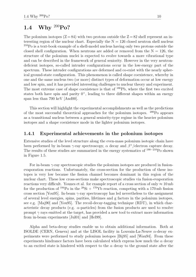
The polonium isotopes (Z = 84) with two protons outside the Z = 82 shell represent an in-teresting region of the nuclear chart. Especially the N = 126 closed neutron shell nucleus210Po is a text-book example of a shell-model nucleus having only two protons outside theclosed shell configuration. When neutrons are added or removed from the N = 126, thestructure of the polonium nuclei is expected to evolve towards a more vibrational typeand can be described in the framework of general seniority. However in the very neutron-deficient isotopes, so-called intruder configurations occur in the low-energy part of thespectrum. These intruder configurations are deformed and co-exist with the nearly spher-ical ground-state configuration. This phenomenon is called shape coexistence, whereby inone and the same nucleus two (or more) distinct types of deformation occur at low energyand low spin, and it has provided interesting challenges to nuclear theory and experiment.The most extreme case of shape coexistence is that of 186Pb, where the first two excitedstates both have spin and parity 0+, leading to three different shapes within an energyspan less than 700 keV [And00].

This section will highlight the experimental accomplishments as well as the predictionsof the most successful theoretical approaches for the polonium isotopes. 200Po appearsas a transitional nucleus between a general seniority-type regime in the heavier poloniumisotopes and a shape coexistence mode in the lighter polonium isotopes.

1.4.1 Experimental achievements in the polonium isotopes

Extensive studies of the level structure along the even-mass polonium isotopic chain havebeen performed by in-beam γ-ray spectroscopy, α decay and β+/electron capture decay.The results of these studies are summarized in the energy systematics of 190−210Po shownin Figure 1.5.

For in-beam γ-ray spectroscopic studies the polonium isotopes are produced in fusion-evaporation reactions. Unfortunately, the cross-section for the production of these iso-topes is very low because the fission channel becomes dominant in this region of thenuclear chart. These low cross-sections make spectroscopic studies via fusion-evaporationreactions very difficult. Younes et al. for example report of a cross section of only ≈ 10 mbfor the production of 194Po in the 28Si + 170Yb reaction, competing with a 170 mb fissioncross section [You95]. In-beam γ-ray spectroscopy has led nevertheless to the assignmentof several level energies, spins, parities, lifetimes and g factors in the polonium isotopes,see e.g. [Maj90] and [You95]. The recoil-decay-tagging technique (RDT), in which char-acteristic decay products (e.g. α-particles) from the fusion products are used to resolveprompt γ rays emitted at the target, has provided a new tool to extract more informationfrom in-beam experiments [Jul01] and [Hel99].

Alpha and beta-decay studies enable us to obtain additional information. Both atISOLDE (CERN, Geneva) and at the LISOL facility in Louvain-La-Neuve α-decay ex-periments were performed to study polonium isotopes [Bij95] and [Wau94]. From theseexperiments hindrance factors have been calculated which express how much the α decayto an excited state is hindered with respect to the α decay to the ground state after the

1.4 Why 200Po? 11

Figure 1.5: Energy systematics of the excited states in the even-mass polonium isotopes.Positive-parity yrast states are denoted by open circles, the asterisks denote the non-yraststates and the bars denote the negative-parity states. Full circles indicate isomeric states.States with the same spin and parity are connected by a line. The figure is taken from[Jul01].

tunneling of the alpha particle through the Coulomb barrier has been taken into account.In addition information on low-lying 0+

2 states has been deduced. Finally, a β-decayexperiment at Louvain-La-Neuve revealed information about the E0 transition in 200Po[Bij95].

Recently, the changes in mean-square charge radii were measured by in-source resonantionization laser spectroscopy at ISOLDE by Cocolios et al. [Coc10]. The results in Figure1.6 show a strong deviation from the predictions of the spherical droplet model starting

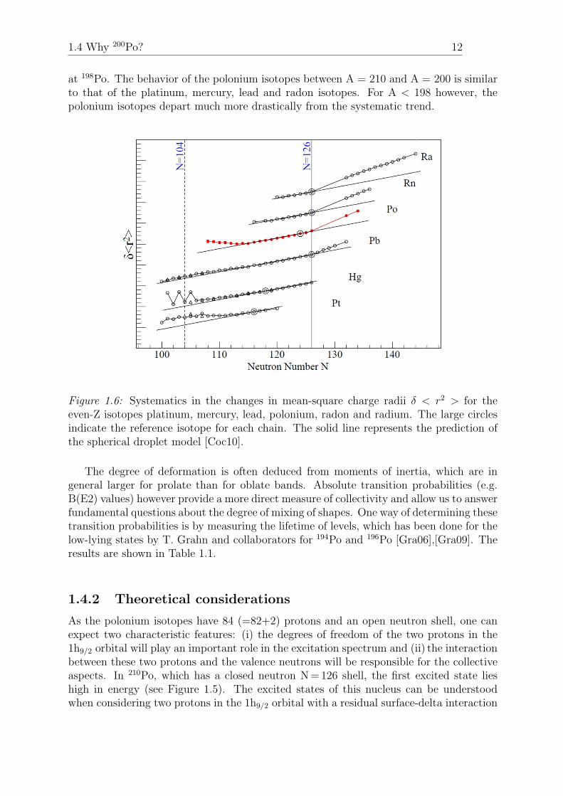
1.4 Why 200Po? 12

at 198Po. The behavior of the polonium isotopes between A = 210 and A = 200 is similarto that of the platinum, mercury, lead and radon isotopes. For A < 198 however, thepolonium isotopes depart much more drastically from the systematic trend.

Figure 1.6: Systematics in the changes in mean-square charge radii δ < r2 > for theeven-Z isotopes platinum, mercury, lead, polonium, radon and radium. The large circlesindicate the reference isotope for each chain. The solid line represents the prediction ofthe spherical droplet model [Coc10].

The degree of deformation is often deduced from moments of inertia, which are ingeneral larger for prolate than for oblate bands. Absolute transition probabilities (e.g.B(E2) values) however provide a more direct measure of collectivity and allow us to answerfundamental questions about the degree of mixing of shapes. One way of determining thesetransition probabilities is by measuring the lifetime of levels, which has been done for thelow-lying states by T. Grahn and collaborators for 194Po and 196Po [Gra06],[Gra09]. Theresults are shown in Table 1.1.

1.4.2 Theoretical considerations

As the polonium isotopes have 84 (=82+2) protons and an open neutron shell, one canexpect two characteristic features: (i) the degrees of freedom of the two protons in the1h9/2 orbital will play an important role in the excitation spectrum and (ii) the interactionbetween these two protons and the valence neutrons will be responsible for the collectiveaspects. In 210Po, which has a closed neutron N = 126 shell, the first excited state lieshigh in energy (see Figure 1.5). The excited states of this nucleus can be understoodwhen considering two protons in the 1h9/2 orbital with a residual surface-delta interaction

1.4 Why 200Po? 13

Eγ [keV] Ii τi [ps] B(E2) [W.u.]194Po 319.7 2+ 37 (7) 90 (20)

366.5 4+ 14 (4) 120 (40)196Po 463.1 2+ 11.7 (15) 47 (6)

427.9 4+ 7.8 (11) 103 (15)499.1 6+ 2.9 (12) 130 (60)

Table 1.1: Results of lifetime measurements on 194Po and 196Po and B(E2) values of thelow-lying states extracted from them [Gra06],[Gra09].

and the breaking of the πh9/2 pair [Ciz97]. In that way, 210Po clearly fulfills expectation(i) as it offers a text book example of a “two-particle nucleus” [Oro99]. Removing twoneutrons makes the 2+

1 state and (to a lesser extent) the 4+1 state drop down in energy.

The 2+1 energy remains approximately constant down to 200Po while the 4+

1 , 6+1 and 8+

1

states show a smooth increase in energy. These low-energy excitations can be associatedwith quadrupole vibrations or by single-particle motion. In the Particle Core Model(PCM) they have been explained by considering two protons coupled to a vibrating Pb-core [Oro99],[Ciz97]. The parameters involved in doing the PCM calculations are theproton-proton interaction strength, the phonon energy and the strength of the proton-core interaction. Figure 1.7 shows the comparison of the PCM calculated states with theexperimental states. The PCM reproduces the yrast states and the 4+

2 and 6+2 states as

showed in Figure 1.7. The 2+ and 4+ level are explained as a one and two-phonon staterespectively, the 6+ and 8+ states are considered pure zero-phonon excitations (π(1h9/2)2).The energy systematics of the excited 0+ state could not be explained in the frameworkof the Particle Core Model and it was suggested that these levels are more collective thanthe PCM calculations suggest.

The 200Po nucleus seems to mark the end of this regular seniority-type regime. From198Po onwards, an abrupt downsloping trend for the excited states with spin I≤ 6 is ob-served. In Figure 1.7 shows the experimentally observed trend is reproduced in 192−198Pobut in order to do so the proton-core interaction strength has to be increased sharply. Oroset al. argue against the unphysically sharp rise in the proton-core interaction strengththat was used by Cizewski and Younes. They concluded that one cannot describe theenergy systematics of the 192−198Po isotopes using an anharmonic vibrator framework bykeeping the PCM parameters in a physically meaningful range [Oro99].

Furthermore the near-degeneracy of the 6+1 and the 8+

1 state is lifted when goingfrom 200Po to 198Po. From the measured reduced transition probabilities B(E2), the halflifes T1/2 and the g factors of these states conclusions can be drawn about their nature(see Table 1.2). As the B(E2;8+

1 → 6+1 ) changes suddenly between 200Po and 198Po and

g(8+1 ) stays rather constant, it is assumed that the 6+

1 state changes from a predominanttwo-proton structure π(1h9/2)2 to a likely vibrational character while the 8+

1 state keepsits two-proton character. This can be associated with an increase in the collectivity ofthe low-lying states because of the increasing number of valence neutrons. While thecollectivity “reaches” the 6+

1 state, the 8+1 state is not affected [Oro99].

1.4 Why 200Po? 14

Figure 1.7: Results of Particle Core Model calculations compared to the experimentalstates for a) the yrast levels and b) the non-yrast levels in 194−208Po. The solid linesrepresent the PCM predictions while the circles represent the experimental values. To beable to reproduce the trend in 194−198Po the strength of the proton-core interaction hadto be increased [Ciz97].

198Po 200PoT1/2(8+

1 ) [ns] 29 (2) 61 (3)Eγ(8

+1 →6+

1 ) [keV] 136.1 (2) 12.2 (2)B(E2;8+

1 →6+1 ) [e2fm4] 137 (10) 655 (35)

g(8+1 ) +0.91 (3) +0.93 (2)

Table 1.2: Half lifes T1/2, energies Eγ , reduced transition probabilities B(E2) and g factors of198Po and 200Po. The data are taken from [Maj90].

The 2+2 and 4+

2 states in 196,198Po can be interpreted in two ways. Alber et al. sug-gest them to be members of a collective π(4p2h) band that is the product of a protonpair excitation across the Z = 82 shell [Alb91]. Bernstein et al. offer an alternative ex-planation by comparing energy ratios of excited stated and ratios of B(E2) values fordecay from the 4+

2 and 2+2 states in 196,198Po to the theoretical predictions for π(1h9/2)2,

vibrational and rotational models [Ber95]. The data are best reproduced by the vibra-tional expectations. An evolution is suggested towards an anharmonic vibrator whichis more collective than the vibrator in the 200−208Po isotopes. This collective motion isattributed to the increasing role of the νi13/2 orbital and its overlap with the πh9/2 orbital.

1.4 Why 200Po? 15

Several approaches have been applied in the study of the lightest (A≤ 198) poloniumisotopes. As mentioned before, the Particle Core Model failed to predict the observedenergy systematics of these isotopes when keeping the parameters in a physically mean-ingful range. Alternative predictions have been made using the Pairing Vibration Modelfor the first excited 0+ states by Oros et al. [Oro99]. The building blocks of the PairingVibration Model are pairs of correlated particles and holes coupled to spin 0+, 2+,... Theresults of these calculations suggest that the 0+

2 states are of 4p-2h structure. Poten-tial Energy Surface (PES) calculations support this description and place them on anoblate minimum, which was already predicted by Nilsson-Strutinsky calculations in 1977[May77]. Further, the oblate minimum is predicted to become the ground state in 192Poand a strongly deformed prolate minimum is predicted to appear as the ground-stateconfiguration in 186Po as shown in Figure 1.8.

Figure 1.8: Summary of the predictions of the Potential Energy Surface calculations for184−202Po. The energy of the 0+ states are plotted accompanied by their respective de-formation parameters β2. Negative values of β2 represent an oblate deformation, positivevalues a prolate deformation [Oro99].

With their self-consistent calculations based on the HF + BCS method Smirnova etal. showed that the lowest 0+

1 and 0+2 states in the lightest Po isotopes do not have

a well defined deformation [Smi03]. Oblate, spherical and prolate shapes are stronglymixed as can be seen on the deformation energy curves in Figure 1.9. Mixing amplitudesconfirming these predictions for the 0+

1 , 2+1 and 4+

1 states in 192−200Po have been deducedfrom two-level mixing calculations by Van de Vel and can be seen in Table 1.3 [vdV03].

Recently self-consistent mean-field calculations have been applied to calculate the exci-tation spectra and transition moments of low-lying states in 194Po and 196Po [Gra08],[Gra09].The results for 194Po are presented in Figure 1.10. After configuration mixing three coex-isting low-lying collective structures at small deformation result. The calculated ground-state wave function is nearly equally distributed around these three structures, with aslight enhancement on the oblate side. Further, a vibrational structure built on theground state and an oblate band are predicted. The calculations performed for 196Po sug-

1.4 Why 200Po? 16

Figure 1.9: Deformation energy curves for the 188−198Po isotopes obtained from con-strained HF+BCS calculations [Smi03].

APo 0+1 2+

1 4+1

sph. [%] obl. [%] sph. [%] obl. [%] sph. [%] obl. [%]192 55 45 8 92 0 100194 74 26 5 95 4 96196 86 14 54 46 20 80198 96 4 84 16 38 62200 96 4 90 10 73 27

Table 1.3: Mixing amplitudes for the lowest 0+1 , 2+

1 and 4+1 states in polonium nuclei

deduced in a two-level mixing model from the level energy systematics of these isotopes[vdV03].

gest a similar picture as can be seen on Figure 1.11. The resulting mean-field deformationenergy surface is extremely soft as a function of the deformation parameter. The coexis-tence of a spherical-vibrational structure built on the ground state and an oblate band issuggested. Finally, the contributions of the oblate component to the mixing amplitudesfor the ground state in 194,196Po obtained from these calculations are much bigger thanthe ones that were predicted by Van de Vel (see Table 1.3).

From all this, it can be suggested that in the lightest polonium isotopes the interplayof spherical and deformed structures, which are strongly lowered in energy as the numberof neutrons decreases, is responsible for the observed perturbation of the systematics.Figure 1.5 clearly indicates that 200Po is a transitional nucleus. The aim of the presentwork is to study this nucleus via Coulomb excitation.

1.5 Why Coulomb excitation? 17

Figure 1.10: Left: Mean-field and angular-momentum projected deformation energycurves for J ≤ 8 in 194Po as a function of the intrinsic deformation β2 of the mean-fieldstates together with selected collective states plotted at the average intrinsic deforma-tion of the states they are constructed from. The energy scale is normalised to the 0+

ground state obtained after configuration mixing. Upper right: Collective wave functionsof 2+ − 8+ states in the oblate band. Lower right: Collective wave functions of lowest 0+

states [Gra08].

Figure 1.11: Results from mean-field calculations on 196Po. For more explanation, seecaption of Figure 1.10 [Gra09].

1.5 Why Coulomb excitation?

The level structure along the even-mass polonium isotopic chain has been studied thor-oughly. The heavier polonium isotopes display a general seniority-type character whilein the lightest polonium isotopes experimental evidence suggests the coexistence of sev-eral types of deformation. Important questions remain however concerning the transitionbetween these two modes, which is expected to lie around 200Po, the sign of the defor-mation and the magnitude of the mixing between different configurations. The reducedtransition probability B(E2, 0+

1 → 2+1 ) renders a direct measure of collectivity and insight


in the mixing of shapes. To date, the experimental B(E2) value has been measured onlyfor 194Po [Gra06], 196Po [Gra09] and 210Po [Ell73]. For this work the technique of safeCoulomb excitation has been used to extract the B(E2) value for 200Po. The main featuresof Coulomb excitation are discussed in this section.

1.5.1 Kinematics

The scattering of a projectile nucleusApZp

Y on a target nucleus AtZt

X is described by thetime dependent Schrodinger equation

i~∂

∂t|Ψ(t)〉 = (H0 + V (−→r (t)))|Ψ(t)〉

where V (−→r (t)) is the electromagnetic interaction, which can be decomposed in its mul-tipole components. The classical Rutherford scattering process, where the nuclei scatterelastically, is described by the monopole-monopole part. The monopole-multipole com-ponents induce inelastic scattering, which is also called Coulomb excitation. Through theexchange of the virtual photon of the electromagnetic interaction one (or both) of thenuclei get excited. The differential cross section for the Coulomb excitation process isgiven by

dσclxdΩ

=dσRuthdΩ

· P (i→ f) =(a

2

)2 1

sin4(ϑp2

)· P (i→ f) (1.6)

where P (i→ f) is the probability that the nucleus gets excited by exchange of the virtualphoton and dσRuth

dΩis the differential cross section for Rutherford scattering with

a =ZpZtECM

e2

4πε0

(1.7)

where Ap and At are the masses of the projectile and target nuclei, Zp and Zt are themass numbers of the projectile and target and ECM is the beam energy in the center-of-mass frame in MeV. ϑp is the scattering angle of the projectile in the center of massframe. Figure 1.12 shows the scattering process with 200Po as projectile and 104Pd astarget schematically. 200Po is a radioactive nucleus with a half-life of 11.51 minutes andcan thus not function as target in the Coulomb excitation experiment. The expression“inverse kinematics” is used when the projectile excitation is studied instead of the targetexcitation.

Working in the center-of-mass frame simplifies the calculations. As can be seen onFigure 1.12 there is a simple relationship between the scattering angles for projectile andtarget in the center-of-mass frame: ϑp = π − ϑt. This can be understood intuitively: inthe frame where the center of mass is at rest the total momentum equals zero, hencethe projectile and target nuclei will be scattered “back to back”. Therefore calculationsconcerning scattering processes are almost exclusively performed in the center-of-massframe. The laboratory scattering angle θp can be transformed into the center-of-massscattering angle ϑp by:

tan(θp) =sin(ϑp)

cos(ϑp) + τ(1.8)


Figure 1.12: Schematic representation of the Coulomb-excitation process. θP and θTare the laboratory scattering angles of the projectile and the target, ϑP and ϑT are thecenter-of-mass scattering angles of the projectile and target [Bre06].

with

τ =mp

mt

√Ep

Ep −∆E(1 +mp/mt)

where ∆E is the excitation energy of the nucleus due to Coulomb excitation [Ald75].

1.5.2 Cross section of Coulomb excitation

If the inelastic part of the interaction between projectile and target is weak (i.e. if theexcitation probability is small compared to unity), the excitation probability P (i → f)can be computed using first-order perturbation theory. The result links the excitationprobability with the B(E2) value:

P (i→ f) ∼ f(B(E2, 0+1 → 2+

1 ),Ep). (1.9)

Details of the calculation can be found in the literature [Ald75]. Figure 1.13 shows thecalculated cross section for the elastic (Rutherford scattering) and inelastic (Coulombexcitation) process as well as the excitation probability P (i → f) as a function of thecenter-of-mass scattering angle. Rutherford scattering is strongly enhanced in the forwarddirection because of the 1

sin4(ϑp/2)term in equation 1.6. The Coulomb excitation cross

section does not show this diverging character.

The interaction between projectile and target causes local electric and magnetic fieldsto be created which can become considerably large because of the high incident energy ofthe projectile. These electric and magnetic fields cause the 2+ level for example to be splitinto its magnetic substates. This splitting depends on the magnitude of the electric andmagnetic fields but also on the magnitude and the sign of the quadrupole moment of the 2+


Figure 1.13: This figure shows the differential cross section for Rutherford scattering andfor Coulomb excitation and the excitation probability P (i→ f) for 200Po on 104Pd . Thecross sections were calculated using the code “CLX” (see 1.5.4). The input values wereEp = 2.85 MeV/A, E(2+

1 ) = 666 keV and B(E2, 0+1 → 2+

1 ) = 1.08 e2b2.

state and equals zero when the quadrupole moment is zero. The final state of the Coulomb-excitation process can now be each of the substates of the 2+ state. After Coulombexcitation to one of these sub states, transitions between the sub states themselves canalso come into play rendering a special kind of two-step Coulomb excitation. Second-orderperturbation theory describes the effect of the interference between the one and two-stepCoulomb excitations. This second-order effect is called the “reorientation” effect as thedifferent sub states each represent a different orientation of the nuclear spin of the excitedstate. This change in nuclear spin direction affects the angular distribution of the emittedγ rays and the amount of excitation. In second order the excitation probability for atransition from a 0+

1 to a 2+1 state is given by

P2+1∝ |〈2+

1 ||E2||0+1 〉|2 ·

(1 + 〈2+

1 ||E2||2+1 〉 ·K(θ,Ep)

)(1.10)

whereK(θ,Ep) is a function which strongly depends on the scattering angle and 〈2+1 ||E2||2+

1 〉is the reduced matrix element that links the 2+

1 state to itself via the quadrupole oper-ator [Ald75]. This “diagonal” matrix element is related to the spectroscopic quadrupolemoment of the 2+

1 state:

〈2+1 ||E2||2+

1 〉 =1

0.7579Q.

The influence of the diagonal matrix element on the cross section for Coulomb excitationis detectable if the term 〈2+

1 ||E2||2+1 〉 · K(θ,Ep) is comparable to (or larger than) 1.

Practically this means that the value of the diagonal matrix element should be on theorder of 1. The second-order effect is illustrated in Figure 1.14 where the differentialcross section for Coulomb excitation is shown as a function of the center-of-mass anglefor different values of the diagonal matrix element.

The Coulomb-excitation theory is only valid when nuclear effects do not influence thescattering process. Nuclear effects can come into play when the closest distance between


Figure 1.14: Differential cross section for Coulomb excitation for 200Po on 104Pd for dif-ferent values of the diagonal matrix element calculated with CLX. The input values werethe same as in Figure 1.13 but a value for the diagonal matrix element was added.The values that are used for the diagonal matrix element are 〈2+

1 ||E2||2+1 〉 = 0.4 eb,

〈2+1 ||E2||2+

1 〉 = 0 eb and 〈2+1 ||E2||2+

1 〉 = −0.4 eb respectively.

the projectile and the target becomes comparable to the range of the strong interaction (afew fm). When the excitation process is purely electromagnetic the term “safe” Coulombexcitation is used. In order to ensure that nuclear effects don’t contribute, the distance ofclosest approach of the nuclei has to exceed a certain minimal distance. The distance ofclosest approach is a function of the beam energy and the center-of-mass scattering angle

b(ϑ) = a(

1 +1

sin(ϑp/2)

)with a given by 1.7. The dependence of b on the beam energy can be easily understood.As both nuclei are positively charged they experience an electromagnetic repulsion whenapproaching each other. In order for the projectile to come closer to the target, theprojectile has to overcome the Coulomb barrier of the target. The higher the beam energy,the closer the projectile and target approach each other. For safe Coulomb excitation it isrequired that the distance of closest approach is at least the sum of the radii of projectileand target, plus the range of the strong interaction

b ≥ bsafe = Rp +Rt + ∆

with ∆ ≈ 5 fm. The radius of a nucleus can be calculated by R = 1.25A1/3 fm [Cli86].Figure 1.15 shows the distance of closest approach in function of the center-of-mass anglefor the Coulomb excitation process of 200Po on 104Pd for two different beam energies. TheCoulomb excitation process is safe for every center-of-mass angle with a beam energy of2.85 MeV/A. However when the beam energy is increased to 4.85 MeV/A the process issafe only for small scattering angles.


Figure 1.15: The distance of closest approach b between projectile 200Po and target 104Pdin fm in function of the center of mass scattering angle θCM for two different beam energies.The red line shows the minimal distance for safe Coulomb excitation.

1.5.3 Application to the experiment

The inelastically scattered nuclei will de-excite through the emission of a γ ray. For thiswork the de-excitation γ rays were detected with the MINIBALL Germanium DetectorArray (more details in section 2.4). The detected number of γ rays is a measure for theexcitation probability to that state if there are no other decay or feeding paths from orto the state. As mentioned before, the excitation probability is proportional to the B(E2)value. By counting the number of de-excitation γ rays information on the B(E2) valuecan thus be extracted. The number of de-excitation γ rays from the first excited state tothe ground state in 200Po is given by

NPoγ (2+

1 → 0+1 ) = εMB,Po · σE2,Po ·

ρdNA

A·NPo (1.11)

where εMB,Po is the total photopeak efficiency of the MINIBALL detector at the energyof the 2+

1 state in 200Po, σE2,Po is the total detected cross section for Coulomb excitationto the 2+

1 state (i.e. the events that create a signal in the particle detector and in thegamma detector), ρd is the target thickness in mg/cm2, NA is Avogadro’s number, A isthe mass number of the target and NPo is the total number of incoming 200Po nuclei. Asthe polonium beam is a weak radioactive ion beam and as the beam intensity fluctuatesthroughout the experiment the total number of incoming 200Po nuclei is not accuratelyknown. Therefore the number of γ rays must be measured relative to the number of γrays corresponding to the de-excitation of the target, of which the Coulomb excitationcross section is known with a good precision. The number of de-excitation gamma raysof the target is given by

NPdγ (2+

1 → 0+1 ) = εMB,Pd · σE2,Pd ·

ρdNA

A·NPo. (1.12)


Dividing 1.11 by 1.12 results in the relative comparison of the beam and target excitation:

NPoγ (2+

1 → 0+1 )

NPdγ (2+

1 → 0+1 )

=εMB,Po

εMB,Pd

· σE2,Po

σE2,Pd

. (1.13)

1.5.4 Computer codes for the calculation of cross sections

Cross sections for Coulomb excitation processes can be calculated with CLX or withGOSIA. CLX is written by H. Ower and adapted by J. Gerl and uses first-order per-turbation theory [Ald75] to calculate excitation cross sections. The input parametersare

1. the beam energy

2. the mass number A and atomic number Z of projectile and target

3. the energies, spins and parities of the populated states

4. the matrix elements connecting the states that are populated

5. the angular coverage of the DSSSD for the scattered particles in the center-of-massframe.

The CLX output consists of the differential cross section at specified angular mesh points,the excitation cross section to each nuclear level and the elastic cross section. The angulardistribution of the γ rays is not taken into account.

GOSIA is a coupled channels code and is developed at the Rochester university byCzosnyka et al. [Czo08]. A least-squares fit, employing the χ2 method, of the calcu-lated transition yields to experimentally observed transition yields is performed. Thenuclear matrix elements are modified during the fitting procedure. The matrix elementsvary within user-specified limits and stay consistent with known experimental data (e.g.branching ratio’s, lifetimes, ...) The gamma yields and the known matrix elements ofthe target are used to calculate a normalization factor to make the information on theprojectile absolute. In a way, this normalization factor is the unknown beam intensity inequation 1.11. The input to GOSIA is more extensive than the CLX input and consistsof four parts:

1. kinematics (masses, energy, energy loss in target,...)

2. nuclear structure (internal conversion coefficients, lifetimes, energies, spins and par-ities of populated states,...)

3. detector geometry (of particle and gamma detector) and efficiency of gamma detec-tion

4. integration options.

GOSIA outputs the differential cross sections, the matrix elements and the χ2 value.

Chapter 2

Experimental Setup

Experiments with exotic nuclei like 200Po suffer from low beam intensities due to low pro-duction cross sections, short life times and the production of unwanted nuclei. Thereforethe efficiency, intensity and selectivity are the most important features of possible pro-duction techniques [Dup06]. The Isotope Separation On Line (ISOL) technique rendersa possibility to make good-quality exotic beams. The 200Po isotopes for this work wereproduced at the ISOL facility ISOLDE in CERN (Geneva). Thereafter the low-energetic200Po beam was post accelerated to 2.85 MeV/u which led to a total incident energy of570 MeV on the 104Pd target.

In this chapter the different parts of the experimental setup are described, startingwith the production of the 200Po nuclei and ending at the detection of the projectile, targetand γ rays emitted after the interaction of projectile and target. Also the extraction ofa γ-efficiency curve is thoroughly described. The final section motivates the use of 104Pdas target.

2.1 Production of the 200Po isotopes

ISOLDE is a radioactive ion beam facility which is situated at the Proton Synchrotron(PS) Booster in CERN. Figure 2.1 shows the layout of the facility schematically. The PSBooster supplies 1.4 GeV protons that impinge on a 238UCx target. The interaction ofthese high-energetic protons with the target induces fission, fragmentation and spallationreactions in the target. In these reactions a wide range of nuclei including a small fractionof 200Po is produced. The reaction products are stopped inside the target material andeventually move out of the target and towards the transfer line by diffusion and effusion.The speed of the diffusion and effusion processes is enhanced by heating the target andtransfer line to a temperature of 2000oC. The elevated temperature also avoids atoms“sticking” to the walls of the target container or the transfer line. Every chemical elementhas a characteristic release time from the target to the transfer line.

The next step in the production process is the ionization of the neutral atoms which isrequired to only select the polonium nuclei and to simplify the post-acceleration process.The perfect ionization mechanism would only ionize the polonium atoms. Three differentionization mechanisms are implemented in the ion sources of the ISOL systems: electron-impact ionization, surface ionization and laser ionization. In this work the polonium

24

2.2 Post acceleration by REX-ISOLDE 25

Figure 2.1: A schematic layout of the radioactive ion beam facility ISOLDE.

atoms were excited to the 1+ charge state by resonant laser ionization in the ResonantIonization Laser Ion Source (RILIS). Information on the different atomic levels in polo-nium is essential for the resonant laser-ionization process to be successful. During theprocess the atoms are excited stepwise by laser photons leading finally to the continuum,to auto-ionizing states or to highly excited states close to the continuum. The ionizationscheme that was used for the polonium isotopes [Coc04] is shown in Figure 2.2. Becauseof the resonant nature of two of the three steps, the ionization process is very efficientand chemically selective. Elements with a small ionization potential can get ionized bycollisions of the atoms with the surface and constitute the (negligible amount of) contam-ination in the beam.

The ions that are created in the ionization process are extracted from the RILIS by anextraction electrode of 60 keV. The beam now consists of the different polonium isotopesand an amount of contamination. After extraction from the ion source the low-energyion beam is mass separated by an analyzing magnet. The mass separation selects theisotopes with mass number A = 200.

2.2 Post acceleration by REX-ISOLDE

In a next step the low-energetic, isobaric and singly-charged beam is delivered to REX-ISOLDE where it is bunched, charge bred and post accelerated in an efficient way in foursteps.

1. The Penning trap cools and bunches the continuous beam. The ions are “captured”by a combination of electric and magnetic fields and in this way decelerated from

2.3 Time structure 26

Figure 2.2: The ionization scheme that has been used to ionize the polonium atoms. Thelast step (510.6 nm) is not resonant. The Ionization Potential (IP) of polonium lies at8.4168 eV [Ril10].

60 keV to several eV. Inside the Penning Trap the ions are decelerated further bycollisions with a dilute buffer gas (argon or neon under a pressure of ≈ 10−3 mbar).Unfortunately the buffer-gas atoms can also be a source of contamination.

2. The singly-charged ions are charge bred by electron-impact ionization at the Elec-tron Beam Ion Source (EBIS). An electron gun provides a 3-6 keV electron beam totransform the 1+ ions into n+ ions. The charge multiplication of the ions serves tosimplify the acceleration process. As the electron-impact ionization technique is notselective, buffer-gas atoms will also get ionized. A distribution of differently-charged200Po is obtained.

3. In the next step the beam is again injected into a mass separator in order to reducethe amount of contamination. The mass separator uses electromagnetic fields toselect ions with the required mass-to-charge ratio A/q (with A the mass numberand q the charge of the ion). In order to select the 200Po48+ ions the A/q value wasset to 4.17.

4. Finally the ions are post accelerated to 2.85 MeV/u in the REX linear accelerator(linac). The total incident energy which the polonium ions hit the palladium targetwith thus equals 570 MeV. The left panel of Figure 2.3 shows the the REX linacwhich consists of three parts.

2.3 Time structure

The experimental setup at REX-ISOLDE has a specific time structure that has to betaken into account during the analysis of the data. In Figure 2.4 the relevant timing

2.4 The detection system 27

Figure 2.3: Left: The linear accelerator at REX-ISOLDE that consists of three parts.The ions move in the direction of the arrow. Right: After the post acceleration the ionsare deflected into the Miniball detection setup [vdW06].

signals related to the REX-ISOLDE operation are shown schematically. The beam isproduced in bunches and not in a continuous way. The PS booster delivers proton pulsesto ISOLDE with a periodicity of 1.2 s. In total 12 of those proton pulses are combined intoa “supercycle” of 14.4 s. The Penning Trap transforms the continuous signal into shortbunches that are injected into EBIS where the charge breeding time was set to 250 msfor this experiment. EBIS produces a bunched signal that is transported to the linearaccelerator. In the linac the beam is accelerated by a voltage that is changing in timewith a resonant frequency.

2.4 The detection system

A bending magnet changes the trajectory of the post-accelerated 200Po ions to let themimpinge on the 104Pd target with a thickness of 2 mg/cm2 as can be seen on the rightpanel of Figure 2.3. After the collision between the projectile and the target both nucleiare scattered (either elastically or inelastically) onto a double-sided silicon-strip detector(DSSSD) which is mounted in the target chamber (see Figure 2.5). If one of the nuclei getsCoulomb excited the de-excitation gamma rays are detected by the Miniball γ-detectorarray that surrounds the target chamber in close geometry to increase the total detectionefficiency. This section describes the Miniball gamma detector, the efficiency of the gammadetection and the particle detector.


Figure 2.4: Time structure of REX-ISOLDE [Hab00].

2.4.1 The Miniball γ-detector array

The Miniball detector array (see Figure 2.6) consists of 8 cluster detectors of which only7 were working in the experiment for this work. Each of the clusters contains threeindividually encapsulated HyperPure Germanium (HPGe) crystals which are surroundedby an aluminium cap. The nuclei that are Coulomb excited will de-excite by emitting agamma ray in flight. Hereby the energy of the gamma ray will be Doppler shifted. In orderto be able to correct for this Doppler shift, the exact positions of the emitting particleand emitted gamma ray have to be known (see section 3.4.1). Therefore it is importantthat the gamma detector is position sensitive. To achieve this position sensitivity, thecrystals are divided into six segments and one central electrode. A total segmentationof 126 (= 7.3.6) was achieved in this way. As the optimal working temperature for thecrystals is low, the crystals are mounted on cold fingers on liquid nitrogen temperature(≈ 70 K). Finally the clusters are placed on four flexible aluminum arms so they can bepositioned in the theta (angle with the beam axis), phi (cone around the beam axis) andalpha (spin around the cluster center) directions.


Figure 2.5: Schematic overview of the Miniball detection setup. The scattered projectileand target fall onto the position-sensitive double-sided silicon-strip detector. The de-excitation gamma rays are detected by the Miniball detector array of which only 7/8th

was working during the 200Po run [Bre10].

Figure 2.6: The Miniball γ detector is placed in close geometry around the target that isplaced inside a metal ball [Dir07].

2.4.2 Efficiency of the γ detection

An absolute efficiency curve for the Miniball gamma detector as it was during the ex-periment for this work (IS479 September 2009, CERN) was extracted by analyzing thegamma spectra taken with a 152Eu source of which the absolute intensity was unknownand a mixed 133Ba/241Am source with respective absolute intensities of 25.76/,kBq and40.11/,kBq. 152Eu decays by β+/EC to 152Sm and by β− decay to 152Gd, 133Ba decaysby β+/EC to 133Cs and 241Am α decays to 237Np. The second source was included inthe analysis because its low-energy gamma rays allow to extract the absolute efficiencyat low energy as well. This section explains the different steps in extracting an absoluteefficiency curve from these two data sets. In a first step the relative detection efficiencies


of the gamma rays of the two sources are calculated. Further using coincidence dataabsolute efficiencies for certain transitions are extracted in the next step. Finally theabsolute efficiency curve is obtained by fitting the absolute efficiency points separately fortwo energy regimes: the energies below 200 keV and the energies above 200 keV.

Relative efficiencies

Figure 2.7 shows the γ spectrum from the decay of 152Eu. Values for the relative detectionefficiencies of the different gamma rays can be calculated by dividing the integrals of thephoto peaks by the corresponding relative intensities1[Chu99]. Exactly the same can bedone for the mixed 133Ba/241Am source (see Figure 2.8). The obtained relative efficiencies(with corresponding errors) are given in Table 2.1. As there was only one transition inthe decay of 241Am observed, at this point it is not possible to extract a value for therelative efficiency at 59.54 keV.

152Eu 133Ba-241AmEγ [keV] εrel Eγ [keV] εrel

121.78 42.41 (10) 80.90 10.96 (8)244.70 32.11 (13) 223.24 9.49 (59)295.94 32.30 (97) 267.40 8.11 (5)344.28 28.24 (43) 302.85 7.94 (4)411.12 23.47 (17) 356.01 7.44 (3)443.96 23.69 (24) 383.85 7.26 (4)778.90 17.90 (5)867.38 15.66 (11)964.07 15.97 (4)1086.38 15.24 (5)1112.04 14.97 (4)1408.01 13.00 (3)

Table 2.1: This table shows the calculated relative efficiencies for the gamma rays in 152Euand 133Ba. The relative efficiencies are expressed in arbitrary units and are multipliedby an arbitrary factor, here 10−4. This table allows a comparison between the relativeefficiencies of the different γ transitions of one source. The relative efficiencies of the twodifferent sources can not yet be compared to one another.

Absolute efficiencies

When considering a gamma cascade as showed in Figure 2.9 the detection efficiency of γ1

and γ2 can be calculated by counting the number of γ2 transitions that are in coincidencewith γ1. The detection efficiency for γ1 is given by

εγ1 =Nγ2γ1(1 + αγ1)

67Nγ2Iγ1(1 + αγ1)

E2→...∑i

(Iγi(1 + αγi)

)(2.1)

1The relative intensity is defined in this case as the theoretical number of gamma rays per 100 decays.


200 400 600 800 1000 1200 1400 1600 1800 200010

210

310

410

510

142

7)±

121.

78 (

1212

130

736

)±

244.

70 (

2434

58

403

)±

295.

94 (

1443

8 9

67)

±34

4.28

(74

8280

368

)±

411.

12 (

5243

2 4

12)

±44

3.96

(74

579

559

)±

778.

90 (

2316

26

372

)±

867.

38 (

6648

5

548

)±

964.

07 (

2353

78 496

)±

1086

.38

(185

638

503

)±

1112

.04

(206

969

532

)±

1408

.01

(273

138

Gamma energy [keV]

Nu

mb

er o

f co

un

ts /k

eV

Figure 2.7: The gamma-energy spectrum from the decay of 152Eu with the number ofcounts on a logarithmic scale. The peaks that have been used in the analysis are denotedwith the gamma energy and the integral of the photo peak. Some clear gamma peaksare not used because they coincide with background radiation from the radioactive decayof the beam or its daughters used in the Coulomb excitation experiment (this gammaspectrum is taken after the Coulomb excitation experiment), e.g. the 367.79 keV gammaray due to the β− decay of 152Eu coincided with the 367.94 keV gamma ray due to thedecay of 200Tl to 200Hg. When two or more gamma rays lie too close in energy to beseparated, the energy that is mentioned is the weighted average of the peaks, e.g. thegamma rays at 963.39 keV and at 964.08 keV yield an average value of 964.07 keV.

where Nγ2γ1 is the number of γ2 transitions observed in coincidence with γ1, αγ1 is thetotal internal conversion coefficient of γ1, Iγi(1 + αγi) is the total relative intensity of γiand the summation runs over all the paths that depopulate energy level E2 (including γ2).The correction factor 6/7 accounts for the fact that if a γ ray hits a crystal in a triplecluster, the same triple cluster cannot register a coincident γ ray (this is a consequenceof the way the data are registered). Also due to the add-back procedure, gamma rayswith an energy above 100 keV are summed when incident within the same cluster. Thiscan be understood as the whole cluster being “blocked” for detection of the coincidentgamma ray. With 7 working Miniball clusters, this leaves 6 available clusters to registerthe coincident gamma ray. However, when considering coincidences with the 80.90 keVgamma ray in 133Ba the correction factor will be 20/21 in stead of 6/7 due to the absence


0 200 400 600 800 1000

210

310

410

510

610 8

73)

±59

.54

(453

912

753

)±

80.9

0 (4

0216

4

261

)±

223.

24 (

4269

321

)±

276.

40 (

5808

4 4

33)

±30

2.85

(14

5463

702

)±

356.

01 (

4617

36

271

)±

383.

85 (

6488

7

Gamma energy [keV]

Nu

mb

er o

f co

un

ts /k

eV

Figure 2.8: The gamma energy spectrum due to the decay of 133Ba and 241Am with thenumber of counts on a logarithmic scale. The peaks that have been used in the analysisare denoted with the gamma energy and the integral of the photo peak. When two ormore gamma rays lie too close in energy to be discriminated, the energy that is mentionedis the weighted average of the peaks, e.g. the gamma rays at 79.61 keV and at 81.00 keVyield an average value of 80.90 keV.

Figure 2.9: A gamma cascade. If the lifetime of level E2 is short enough (< µs) γ1 andγ2 are seen in coincidence.

of add-back. The detection efficiency for γ2 looks similar:

εγ2 =Nγ2γ1(1 + αγ2)

67Nγ1Iγ2(1 + αγ2)

E2→...∑i

(Iγi(1 + αγi)

). (2.2)


Equations 2.1 and 2.2 can then be used to calculate the absolute detection efficiency ofboth γ rays in a cascade. In the β+/EC decay of 152Eu to 152Sm for example the 121.78 keV2+

1 → 0+1 gamma is coincident with the 244.70 keV 4+

1 → 2+1 gamma ray. In the next step

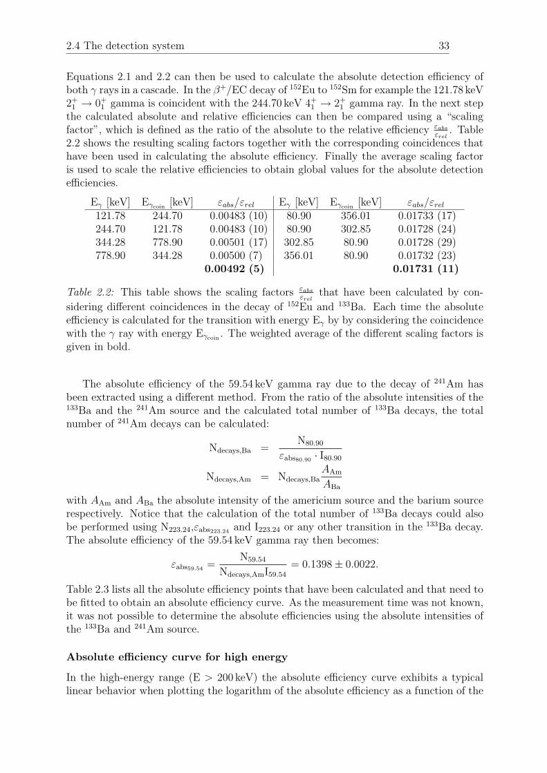
the calculated absolute and relative efficiencies can then be compared using a “scalingfactor”, which is defined as the ratio of the absolute to the relative efficiency εabs

εrel. Table

2.2 shows the resulting scaling factors together with the corresponding coincidences thathave been used in calculating the absolute efficiency. Finally the average scaling factoris used to scale the relative efficiencies to obtain global values for the absolute detectionefficiencies.

Eγ [keV] Eγcoin [keV] εabs/εrel Eγ [keV] Eγcoin [keV] εabs/εrel121.78 244.70 0.00483 (10) 80.90 356.01 0.01733 (17)244.70 121.78 0.00483 (10) 80.90 302.85 0.01728 (24)344.28 778.90 0.00501 (17) 302.85 80.90 0.01728 (29)778.90 344.28 0.00500 (7) 356.01 80.90 0.01732 (23)

0.00492 (5) 0.01731 (11)

Table 2.2: This table shows the scaling factors εabsεrel

that have been calculated by con-

sidering different coincidences in the decay of 152Eu and 133Ba. Each time the absoluteefficiency is calculated for the transition with energy Eγ by by considering the coincidencewith the γ ray with energy Eγcoin . The weighted average of the different scaling factors isgiven in bold.

The absolute efficiency of the 59.54 keV gamma ray due to the decay of 241Am hasbeen extracted using a different method. From the ratio of the absolute intensities of the133Ba and the 241Am source and the calculated total number of 133Ba decays, the totalnumber of 241Am decays can be calculated:

Ndecays,Ba =N80.90

εabs80.90 · I80.90

Ndecays,Am = Ndecays,BaAAm

ABa

with AAm and ABa the absolute intensity of the americium source and the barium sourcerespectively. Notice that the calculation of the total number of 133Ba decays could alsobe performed using N223.24,εabs223.24 and I223.24 or any other transition in the 133Ba decay.The absolute efficiency of the 59.54 keV gamma ray then becomes:

εabs59.54 =N59.54

Ndecays,AmI59.54

= 0.1398± 0.0022.

Table 2.3 lists all the absolute efficiency points that have been calculated and that need tobe fitted to obtain an absolute efficiency curve. As the measurement time was not known,it was not possible to determine the absolute efficiencies using the absolute intensities ofthe 133Ba and 241Am source.

Absolute efficiency curve for high energy

In the high-energy range (E > 200 keV) the absolute efficiency curve exhibits a typicallinear behavior when plotting the logarithm of the absolute efficiency as a function of the


Eγ [keV] εabs Eγ [keV] εabs

59.44 13.98 (22) 383.85 12.57 (7)80.90 18.98 (14) 411.12 11.55 (14)121.78 20.88 (22) 443.96 11.66 (17)223.24 16.42 (101) 778.90 8.81 (9)244.70 15.80 (17) 867.38 7.71 (10)276.40 14.04 (9) 964.07 7.86 (8)295.95 15.90 (50) 1086.38 7.50 (8)302.85 13.74 (6) 1112.04 7.37 (8)344.28 13.90 (25) 1299.14 6.70 (9)356.01 12.88 (5) 1408.01 6.40 (7)

Table 2.3: This table shows the the calculated absolute efficiencies for the gamma rayscoming from the decay of 152Eu, 133Ba and 241Am.

logarithm of the energyln(ε) = p0 + p1 · ln(E/500).

The energy is divided by 500 to decrease the error on the offset parameter p0. Whenperforming a linear fit to a set of data points, the error on the offset can become quite highwhen the “zero point” (=the intercept with the vertical axis) lies far from the considereddata points. A way to circumvent this problem is to fit as a function of (x − a) with aa value on the x axis close to the x-coordinates of the data points. This way the “zeropoint” is brought artificially closer to the data points, making the error on the offset muchsmaller. Fitting to (x− a) translates to fitting to ln(x/a) in the logarithmic case.

0 200 400 600 800 1000 1200 1400 16000

5

10

15

20

25

30

Energy [keV]

Ab

solu

te E

ffic

ien

cy [

%]

Figure 2.10: The absolute efficiencies of the high energy gamma rays due to the decay of152Eu are fitted with a simple exponential function. The absolute efficiency at 121.78 keVhas been left out of the data set for this fit.


In the case of the absolute efficiencies of the high-energy points in the 152Eu data setthe parameters turn out to be p0 = 2.390 ± 0.007 and p1 = −0.512 ± 0.011 (see Figure2.10). The relative efficiencies of the higher-energy points of the 133Ba data set can thenbe fitted into the absolute efficiencies of the 152Eu data set by using

ln(ε) = p0 − 0.512 · ln(E/500)

as fit function. The slope is demanded to be the same as in the 152Eu fit because therelative efficiencies of the 133Ba data should only be shifted by a constant to becomeabsolute efficiencies. The reason that the relative efficiencies are used for this fit (in steadof the absolute) is to keep the error on the final result as small as possible. The offset p0

is found to be 6.430± 0.009 (see Figure 2.11). The relative efficiencies of 133Ba can nowbe scaled to obtain absolute efficiencies:

ln(εabs) = ln(εrel) + (6.430− 2.390).

0 200 400 600 800 1000 1200 1400 1600

200

400

600

800

1000

1200

1400

1600

1800

2000

Energy [keV]

Rel

ativ

e E

ffic

ien

cy [

a.u

.]

Figure 2.11: The relative efficiencies of the high-energy gamma rays coming from thedecay of 133Ba are fitted with a simple exponential function, demanding that the slope isthe same as in the 152Eu fit of Figure 2.10. The absolute efficiency at 80.90 keV has beenleft out of the data set for this fit.

Now all the absolute efficiency points at energies above 200 keV (i.e. the 152Eu pointsand the scaled 133Ba points) can be fitted together to obtain a curve that describes theabsolute efficiency at energies above 200 keV:

ln(εabs) = 2.391− 0.507 · ln(E/500).

Absolute efficiency curve for low energy

When the absolute efficiencies of the points at lower energy are included, a multi-parameterfit has to be used:

ln(ε) = p0 +p1 · ln(E/200)+p2 · (ln(E/200))2 +p3 · (ln(E/200))3 +p4 · (ln(E/200))4. (2.3)


The efficiency increases for decreasing energies. However at low energies the efficiencyreaches a maximum and decreases again. The shape of this turn-over point at low energiesis determined by the higher-order terms of this multi-parameter fit. The result of this fitis shown in Figure 2.12.

- 2 0 0 0 2 0 0 4 0 0 6 0 0 8 0 0 1 0 0 0 1 2 0 0 1 4 0 0 1 6 0 04

6

8

1 0

1 2

1 4

1 6

1 8

2 0

2 2Ab

solut

e Effic

iency

[%]

E n e r g y ( k e V )

Figure 2.12: All the absolute efficiency points ((i.e. the 152Eu points, the scaled 133Bapoints and the one point due to the decay of 241Am) have been fitted with the multi-parameter fit given in equation 2.3.

Again the energy in the fit function is divided by a constant to reduce the errors on thefit parameters. For this multi-parameter fit it was not clear which division constant wouldgive the best result. Therefore the relative errors on the calculated absolute efficienciesare compared in Figure 2.13. When dividing by 1000, the errors become large, especiallyfor low energies (the zero point lies at high energy!). The opposite effect can be seen whenthe division factor is small, for example when dividing by 10 the relative errors at highenergy become large. A minimal relative error on the absolute efficiencies for all energiesseems to be reached for the fit with ln(E/200).

To obtain a final absolute efficiency curve the linear fit at energies above 200 keV iscombined with the multi-parameter fit at energies below 200 keV (see Figure 2.14).

Input in GOSIA

GOSIA, the programma used for the extraction of matrix elements out of the Coulombexcitation data, also takes the γ-detection efficiency into account. As an input, GOSIArequests the parameters of the fit without errors. As the value of the absolute efficiencyat energies above 200 keV is the same for the multi-parameter fit and the linear fit (onlythe errors vary), the five fit parameters that result from the multi-parameter fit are usedas input for GOSIA. However GOSIA requests the parameters of the general efficiencyformula ln(ε) = p0 +p1 · ln(E) +p2 · (ln(E))2 +p3 · (ln(E))3 +p4 · (ln(E))4 so that equation2.3 needs to be rewritten. The input parameters for GOSIA become:


Figure 2.13: The relative error on the calculated absolute efficiency is shown for a rangeof γ energies in function of the type of fit that was used. The horizontal axis shows thedivision factor x in the fit with ln(E/x). The different curves express the relative erroron the absolute efficiency for different energies. This error is demanded to be as low aspossible for all energies.

Figure 2.14: The final curve expressing the absolute efficiency for every energy. Thiscurve is a combination of the multi-parameter fit at low energy and the linear fit at highenergy.

As the parameters that determine the efficiency curve are included in GOSIA without


p0=-85.048p1= 54.613p2=-13.539p3= 1.470p4= -0.060

errors, the uncertainty on the efficiencies has to be included in the error on the photo-peakintegrals. However, since GOSIA performs a minimization by normalizing the projectileto the target excitation, the error on the constant term p0 can be put to zero. Howeverthis can only be done when comparing two gamma’s lying in the same energy regime.The uncertainty on the fit parameters differs for the linear fit and the multi-parameterfit! When for example comparing the photo peak of a low-energy γ ray to the photo peakof a high-energy γ ray the error on the constant term p0 cannot be simply put to zero.Indeed, the errors on the fit parameters for the two regimes differ.

To circumvent this problem, the following solution is applied. In the calculation of theuncertainty on the efficiency at energies above 200 keV the error on the constant term p0

is put to zero. The only transition at low energy that will be used in the analysis is thepolonium X-ray transition at 79 keV. In order to include the correct error on the efficiencyat this low energy when comparing it to the photo peak of the target excitation, anadditional error is included in the error on the X-ray photo peak. This error is simply theerror on the constant term p0 of the linear fit at high energies. The error on the constantterm p0 that had been put to zero is now artificially brought back into the calculation.Table 2.4 shows the relevant absolute efficiencies with the appropriate (absolute) errorsfor the Coulomb excitation experiment on 200Po.

Eγ [keV] εabs real error GOSIA error79 0.1879 0.0082 0.0084

555.8 0.0945 0.0007 0.0001666.9 0.1036 0.0007 0.0001

Table 2.4: This table shows the values for the absolute efficiencies at three importantenergies: the X-ray energy of polonium and the 2+ → 0+ energy in 104Pd and in 200Po.The real error is the calculated error on the absolute efficiency like in Figure 2.14. Forthe GOSIA error the error on p0 has been set to zero for the points at high energy. TheGOSIA error of the X rays includes the error on p0 of the multi-parameter fit and on p0

of the linear fit.

2.4.3 Double-sided silicon-strip detector

The double-sided silicon-strip detector (DSSSD) that serves as particle detector in thesetup, is mounted in the target chamber at a distance of 32.5 mm from the 104Pd targetand is divided into four independent quadrants as shown in Figure 2.15. The right-handside of the schematic picture shows the layout of the front face, the lower left side showsthe layout of the rear face and the upper left side displays the overlap between the front


and the rear face. Each of the four quadrants consists of a silicon wafer with a thicknessbetween 476 and 481 µm and is divided into 16 annular strips in the front plane and 24sector strips in the rear plane (the latter being coupled electronically into groups of twosector strips). This segmentation makes the DSSSD position sensitive as is required to beable to correct for the Doppler shift of the detected γ energy. For this work the followingnaming convention is used for the annular strips: strip number 0 corresponds to the stripat the largest scattering angle in the laboratory frame (the most outer strip), while stripnumber 15 corresponds to the most inner strip.

Figure 2.15: Left: Schematic picture of the double-sided silicon-strip detector [Ost02].Right: Picture of the double sided silicon strip detector.

From the distance between the target and the DSSSD and the width and pitch of theannular strips we can infer the minimal and maximal detection angles in the laboratoryframe: 15 and 52. As we know the energy and mass of the incoming beam and the massof the target, these laboratory angles can be translated to the center-of-mass frame byusing equation 1.8. The DSSSD ranges from 45 to 139 in the projectile center-of-massframe and from 76 to 149 in the target center-of-mass frame. Figure 2.16 visualizes therelation between the laboratory and the center-of-mass scattering angles. The maximalscattering angle of the 200Po projectile in the laboratory frame is only 31. This reflectsthe fact that the trajectory of the projectile, which is much heavier than the target, isless affected by the collision than the trajectory of the lighter target nucleus.

Figure 2.16 predicts the maximal detection angle in the center-of-mass frame for theprojectile to be 164. However, the energy of the scattered polonium ions has decreasedto 67 MeV at this scattering angle (see Figure 2.17) which is not enough to travel throughthe 2 mg/cm2 palladium target. However, if the scattering between projectile and targettakes place at the end of the target, the polonium ion will probably have enough energyto escape the target. In this case we consider the extreme case where the scattering takesplace immediately when the polonium ion encounters a palladium nucleus. SRIM [Zie10],a programme for the calculation of the stopping and range of ions in matter, shows thatthe energy loss of a 570 MeV 200Po ion inside 104Pd equals 58.77 MeV

mg/cm2 . The total energy

2.5 The 104Pd target 40

Figure 2.16: The scattering angle in the laboratory frame θLAB in function of the scatter-ing angle in the center of mass frame ϑCM for a 200Po projectile and a 104Pd target givenboth for projectile and target. In blue the range of the DSSSD in the laboratory frame isshown.

loss inside the 2mg/cm2 104Pd target thus equals 117.54 MeV.

Figure 2.17: The energy of the projectile and target in the laboratory frame as a functionof the scattering angle in the center of mass frame for a 200Po projectile on a 104Pd target.In blue the minimal energy for the projectile required to be able to travel through the2mg/cm2 target is given.

2.5 The 104Pd target

The choice of the most appropriate target material is a crucial step on the road to asuccessful Coulomb-excitation experiment. First of all the target nucleus has to be stable(which is the case for 104Pd). For the analysis of the gamma spectra it is important


that the energies of the de-excitation gamma rays of projectile and target differ enoughin order for them to be discriminated. From the low-lying energy levels of target andprojectile shown in Figure 2.18 it can be seen that the 104Pd target also fulfills this secondcondition. The third condition concerns the kinematics of the reaction: projectile andtarget nuclei falling on the DSSSD need to be distinguishable. A simulation of the energyof the detected particles in function of the strip number in the DSSSD shows that a cleanseparation between the polonium and palladium nuclei is possible (Figure 2.19). Finallythe target nucleus has to be collective enough in order to observe a sufficient amount oftarget excitation to be able to perform a decent relative comparison between the projectileand target excitation (see equation 1.13). The cross section for Coulomb excitation to thefirst excited 2+ state in 104Pd using a 200Po beam of 2.85 MeV/u was calculated with CLXto be 0.941 b2. Using equation 1.12 a quick calculation teaches that this means roughly105 counts in the 104Pd de-excitation peak which is largely enough3. To conclude 104Pdseems a very appropriate target nucleus.

Figure 2.18: The level scheme of the low lying excited states of 200Po and 104Pd. Thetransitions that are denoted in the level scheme of 200Po are the transitions that havebeen observed in the β+/EC-decay study of 200Po by Bijnens et al. [Bij98].

2For this CLX calculation the known matrix elements connecting the low-lying states in 104Pd havebeen used as input: 〈2+

1 ||E2||0+1 〉 = 0.731 eb, 〈2+

2 ||E2||0+1 〉 = 0.134 eb, 〈2+

1 ||E2||2+1 〉 = −0.62 eb,

〈2+1 ||E2||4+

1 〉 = 1.162 eb, 〈2+1 ||E2||2+

2 〉 = 0.574 eb and 〈0+2 ||E2||2+

1 〉 = 0.2 eb [Luo86],[Fah77],[Ram87].3In this calculation the incoming intensity of the polonium ions was estimated to be IPo ∼ 105s−1 and

the value for the detection efficiency of the 555.8 keV peak was εPd = 10.36 %.


0 2 4 6 8 10 12 14 160

100

200

300

400

500

0

20

40

60

80

100

120

140

160

180

Strip Number

Nu

mb

er of co

un

ts /MeV

/Strip

En

erg

y [M

eV]

Po200

Pd104

Figure 2.19: The simulated number of detected particles in function of the energy and thestrip number for a 200Po projectile on a 104Pd target. In this calculation it was assumedthat the beam was perfectly centered with a beam spot of only 9 mm2.

Chapter 3

Data Analysis

This chapter describes the analysis of the data that are obtained from the Coulombexcitation experiment on 200Po which was performed for this work in September 2009at CERN. A first step in the analysis consists of the energy calibration of the particledetector. A Coulomb excitation event consists of the detection of two coincident particlesin the DSSSD (projectile and target) that are scattered back to back in the center-of-mass frame and the detection of a gamma ray that is in coincidence with these twoparticles as well. In a second step these Coulomb excitation events are selected out of thebackground. The corresponding gamma spectrum, after performing a Doppler correction,is used to extract information on the cross section for Coulomb excitation of 200Po. Finally,using GOSIA, values for the matrix elements connecting the low-lying states in 200Po areobtained.

3.1 Energy Calibration of the DSSSD

A particle that hits the DSSSD will deposit its energy in the silicon wafer and createelectron-hole pairs in this semi-conducting material. An applied electric field makes theseelectron-hole pairs move in opposite direction through the silicon. The magnitude of theelectric current that is generated in this way is after proper signal processing associatedwith a channel number. As the number of created electron-hole pairs is proportionalto the energy of the incident particle, the relation between the channel number and theenergy is linear:

E = a+ b · C (3.1)

with E the energy of the incoming particle and C the associated channel number. Cal-ibrating the DSSSD thus consists of determining the parameters a and b in equation3.1 for every annular strip, every sector strip, per quadrant. This means that in total(16 + 12) ·4 = 112 parameters have to be extracted. To be able to extract a and b at leasttwo energy points are needed.

First, a stable 40Ar beam is accelerated to 2.85 MeV/u (2.85 · 40 = 114 MeV). Thescattering process of these 114 MeV 40Ar nuclei on a 197Pt target was analyzed. Twoprocesses need to be taken into account in calculating the detected energy of the 40Arions. Due to kinematics considerations, the detected energy of the 40Ar particles in theDSSSD will vary with the detection angle. The incident energy of the 40Ar ions varies from

43

3.1 Energy Calibration of the DSSSD 44

98 MeV at the outer strip to 112 MeV at the strip associated with the smallest laboratoryscattering angles. The second effect that has to be taken into account is the energy lossof the 40Ar ions in the 2.0 mg/cm2 197Pt target. This energy loss can be calculated withSRIM [Zie10] and is on average equal to 14 MeV. In fact the incident ions have to travelthrough more than just the actual thickness of the target because of the oblique scattering.To take this effect into account, it was assumed that the scattering process takes placeexactly in the middle of the target. The 40Ar ions travel horizontally through the first1 mg/cm2 of the target and in the middle of the target the 40Ar ions are scattered. Asthe scattering angle is known, the actual energy loss in the target can be calculated. The“real” total energy loss varies from 18.4 MeV in the outer strips to 14.5 MeV in the innerstrips. Figure 3.1 shows the spectrum that was used to calibrate the annular strip thatcorresponds to the largest scattering angle in the laboratory frame of the first quadrant.The 40Ar peak can clearly be seen and is broadened by the energy straggling in the target.

Figure 3.1: This graph shows the number of detected 40Ar ions as a function of thechannel number that was used in the calibration of the outer strip of the first quadrant.The mean channel number of the peak was extracted by fitting the peak with a Gaussianfunction and equals 594. The low-energy part of the peak is due to noise in the detector.

To obtain a second energy point to complete the calibration, the scattering processof the 200Po projectile on the 104Pd target is used. Indeed, the kinematics of this processare completely known as it is a classical scattering process. As the 104Pd target nucleiare detected throughout the complete angular range (see Figure 2.16) of the particledetector the 104Pd points are perfect to use as the second energy point in the calibration.Another advantage of using the 104Pd points for the calibration are the high incident


energies. This way the calibration is based on a point at relatively low energy (40Ar) andon a point at higher energies (104Pd) making an extrapolation to the high energies in theCoulomb-excitation experiment on 200Po unnecessary. To calculate the incident energy ofthe 104Pd ions on the detector, it was assumed that the interaction between projectile andtarget takes place in the middle of the target. The energy loss of the polonium projectilemust be taken into account to calculate the energy with which the palladium nucleus isscattered. Also the energy loss of 104Pd in the second half of the target is included inthe calculation. The detected energy of the 104Pd ions varies from 125 MeV in the outerstrips to 397 MeV in the strips with small laboratory scattering angle. As an example thespectrum corresponding to the most outer strip of the first quadrant is shown in Figure3.2. The 104Pd peak is clearly present and relatively easy to fit as in this strip of theparticle detector no polonium ions are detected. However, finding the 104Pd peak in theparticle spectrum is difficult in strips corresponding to small laboratory scattering angles(large strip numbers). As can be seen in Figure 2.19 the energies of the projectile andtarget are lying close to each other at small laboratory angles. The two peaks will thusoverlap in this angular range.

Figure 3.2: This graph shows number of detected 104Pd ions as a function of the channelnumber that was used in the calibration of the most outer strip of the first quadrant. Themean channel number was found by fitting the peak with a Gaussian and equals 870.

This procedure of calculating the detected 40Ar and 104Pd energies and fitting thecorresponding peaks to find the channel number is repeated for every strip in every quad-rant. Using the obtained channel numbers and energies the parameters a and b can be


calculated as

a = EPd − b · CPd

b =EPd − EAr

CPd − CAr

3.1.1 Problem in strip 8

When plotting the number of counts versus the energy in a single annular strip of thedouble-sided silicon-strip detector, the structure of the spectrum can be predicted bylooking at the result of the simulation in Figure 2.19. In fact the intensity versus energyspectrum for one strip is simply the projection of this plot on the vertical axis. Sucha spectrum for strip number 8 is expected to have two peaks: one peak at high energy(≈ 250 MeV) representing the detection of the 104Pd target and one (smaller) peak atlower energy (< 100 MeV) corresponding to the 200Po projectile. Figure 3.3 clearly showsone additional peak at ≈ 175 MeV in the experimentally obtained spectra for quadrant 1and 2 while the spectra for the two other quadrants seem normal.

Figure 3.3: The number of counts as a function of the particle energy for strip number 8.The different panels show the spectrum for each of the 4 quadrants of the DSSSD. Thesespectra only show the events where two prompt particles are detected that are scatteredback to back in the center-of-mass frame.

The origin of this unexpected peak can be investigated by plotting the energy versusstrip number of the particles that are in coincidence with the particles in the different

3.2 Two-particle events 47

peaks. Figure 3.4 shows the spectra corresponding to the three peaks in the spectrum ofquadrant 1. The upper right panel of this figure has been obtained by putting a gate on theparticles in strip 8, quadrant 1 and with energy between 0 and 120 MeV and then plottingthe coincident particles that are scattered back to back in the center-of-mass frame. Thecorresponding energy versus strip spectrum shows the kinematical systematics of 104Pd(see Figure 2.19). This means that the coincident particle must be 200Po. In the same way,by gating on the particles in strip 8 and quadrant 1 with energy between 120 MeV and200 MeV, the lower left panel is plotted and the lower right panel is obtained by gatingon the particles in strip 8 and quadrant 1 with energy between 200 MeV and 350 MeV.These spectra show the kinematical systematics of 200Po and thus must the coincidentparticles be 104Pd. It can be concluded that the first peak of the energy spectrum of strip8 in the first quadrant is due to 200Po while the second and third peak are due to 104Pd.The 104Pd peak is thus split up. Exactly the same procedure can be applied to investigatethe content of the peaks of strip 8 in quadrant 2. Figure 3.5 shows that the first peakcontains a mixture of 200Po and 104Pd and that the 104Pd peak is again split up in twopeaks.

In order to understand the splitting of the palladium peak in quadrant 1 and 2 in strip8 the time evolution of the energy of the detected particles is plotted in Figure 3.6. Thetime steps are discrete because actually the evolution of the detected energy from eachindividual (normalized) run is plotted. It can be clearly seen that the detected palladiumenergy floats in time in quadrant 1 and 2 indicating that something went wrong in theseparts of the particle detector. As the kinematics of the scattering process are known, theycan be corrected for this variation in energy by simply “promoting” the events with a toolow energy to the simulated energy for strip 8.

3.2 Two-particle events

A Coulomb excitation event is constituted of the detection of two particles that arescattered back to back in the DSSSD in coincidence with a gamma ray in the Miniballdetector. The selection of these two-particle events is a powerful tool to separate theprojectile and target in the energy versus strip number plot. This is illustrated in Figure3.7 where the left spectrum is produced by gating on the events in which a particle in theDSSSD and a γ ray in Miniball are in coincidence and the spectrum on the right-handside is obtained by gating on the physical events (coincidence of a γ ray and two particlesthat are scattered back to back). The loss of intensity of the peaks is compensated by again in selectivity.

The motivation for the use of the two-particle method [Bre10] is twofold. Firstly, thekinematics of the scattering process are precisely known. When the two-particle eventsare selected carefully, it is possible to label each detected particle as 104Pd or as 200Po.This information can then be used to explicitly select each time a combination of a 104Pdand a 200Po particle. Hence the two-particle method assures the identification of thecorrect particle for each two-particle event. The second advantage of the two-particlemethod concerns the fact that every selected event is precisely the same. By only taking


Figure 3.4: Upper left: The experimental particle energy spectrum of strip 8 in the firstquadrant. The nature of each peak is extracted from the three other spectra. Upper right:Energy versus strip number when gating on the first peak of the upper left spectrum. Thisshows the kinematics of 104Pd, thus the coincident particle is 200Po. Lower left: Spectrumobtained by gating on the particles in the second peak of the upper left spectrum. Thekinematics of 200Po can be seen, the corresponding particle must thus be 104Pd. Lowerright: Spectrum obtained by gating on the particles in the third peak of the upper leftspectrum. The kinematics of 200Po are observed so the coincident particle is 104Pd.

the two-particle events into account, the conditions for each event are identical. Thereforea correction for the efficiency of the particle detection is not required.

In Chapter 1 it was explained that the cross section for Coulomb excitation dependsin second order on the value of the diagonal matrix element of the first excited state.Figure 1.14 shows that by scanning the angular range of the particle detector, sensitivitycan be achieved on this secondary effect. By comparing the cross sections for Coulombexcitation in different angular ranges of the DSSSD a value for the quadrupole momentcan be obtained. The scanning of the angular range can be performed by “following”the 104Pd particles through the angular range. The 200Po particles only cover the largelaboratory scattering angles because of the backbending in the laboratory frame. The104Pd nuclei on the other hand are scattered throughout the whole angular range. Hencethe 104Pd particles are the perfect “guide” throughout the center-of-mass range. Figure3.8 shows, compared to the simulation, the 104Pd particles that are detected in strip0 (the outer strip) and the particles that are in coincidence with these particles. The


Figure 3.5: This graphs show the same procedure as in Figure 3.4 applied on the energyspectrum of strip 8 in quadrant 2. It can be concluded that the first peak of the spectrumcontains a mixture of polonium and palladium and that the second and third peak bothcontain palladium. For detailed explanation see caption of Figure 3.4.

experimental spectra are consistent with the simulated ones.

In order to select only the physical events, a cut can be made in the 200Po spectrum ascan be seen on the upper-right panel of Figure 3.8. This procedure is repeated for everystrip of the DSSSD. By demanding a coincidence between the 104Pd particles in a certainstrip and the corresponding 200Po particles, the angular dependence of the Coulomb-excitation cross section can be observed. This is done by analyzing the γ spectrum forevery individual strip.

3.2.1 Peak at low energy

Figure 3.9 shows the energy spectra of strips 12, 13, 14 and 15 of the DSSSD (the stripsassociated with the smallest laboratory scattering angles). In each of these spectra a peakat low energy can be seen. The origin of this peak is investigated in this section. A gatehas been put on this peak for each of these spectra to investigate the kinematics of thecorresponding particle (see Figure 3.10). In strips 12 and 13 the peak at ≈ 55 MeV ismainly due to low-energy 200Po particles as the coincident particle exhibits the kinematicsof 104Pd. These polonium particles can be situated on the kinematical plot of Figure 3.7in the 200Po region after the backbending of the laboratory scattering angles. Howeverthe results for strip 14 and 15 show evidence for an additional effect causing this peak as


Figure 3.6: Evolution of the detected energy in strip 8 in time when gating on the two-particle events. To make this plot, only the big runs are taken into account. The runnumbers do not correspond to the real run numbers.

Figure 3.7: Left: Energy versus strip number for all events. Right: Energy versus stripnumber for events with two particles that are scattered back to back in the center-of-massframe (i.e. detected in opposite quadrants of the DSSSD) and are coincident with a γ ray.In both panels the intensity is plotted on a logarithmic scale. The separation betweenprojectile and target is significantly better in the right panel.

the observed kinematics are not simply due to 104Pd.


Figure 3.8: Upper left: the 104Pd particles that are detected in strip 0 when demandingthe detection of two particles that are scattered back to back in the center-of-mass frameand are coincident with a γ ray . Upper right: the particles that are coincident with the104Pd particles in strip 0. A cut is made in this spectrum to select the physical events.Lower panels: simulated 104Pd particles in strip 0 and the corresponding 200Po particles.

A possible alternative explanation for the appearance of this peak at small energy andscattering angle is the scattering of 22Ne gas in the target chamber. As was explainedalready in Chapter 2, the Penning Trap is filled with a dilute buffer gas to slow the atomsdown. The neon atoms from this buffer gas can also be post accelerated and contaminatethe beam. The incident energy of the 22Ne ions is calculated using the mass, the energyloss in the target and the kinematical considerations and is found to be ≈ 52 MeV. Toexamine if the peak at low energy is caused by Rutherford scattering of 22Ne, the low-energy peak has been integrated in the “raw” uncalibrated spectra. The uncalibratedspectra have been used for this integration to increase the statistics. The uncalibratedspectra do not demand any coincidences so they contain all detected events. Also it ispossible that some low-energy events do not exceed the calibration threshold. By usingthe uncalibrated spectra these events are also included. This has been done for all thestrips where the peak is visible and for each quadrant separately. The cross section forRutherford scattering varies as a function of the scattering angle in the center of massframe as 1/sin4(θCM/2) (see equation 1.6). The integrals are plotted as a function of thisangular dependency in Figure 3.11. As the trends are linear, it can be concluded that theintegrals follow the systematics of Rutherford scattering.

3.3 Determination of prompt and random window 52

Figure 3.9: Number of detected particles as a function of the energy for the inner strips ofthe double-sided silicon-strip detector. These spectra only show the two-particle events.

To conclude, the peak at ≈ 55 MeV has a double origin. Firstly the peak can beexplained by low-energy 200Po particles hitting the DSSSD at small laboratory scatteringangles. The second effect is the Rutherford scattering of 22Ne contaminants. To quantifythis analysis the following procedure is applied. The kinematics simulation learns thatthe 200Po particles at low energy (the particles in the back-bending region) are coincidentwith 104Pd particles in strip 9 until 15. Hence, by gating on the palladium particles instrip 9 until 15 and by integrating the corresponding polonium peak at low energy, a valuecan be extracted for the fraction of polonium particles to neon particles in the low-energypeak. The results are listed in Table 3.1 and confirm what was expected. The amount of22Ne Rutherford scattering is by far the most important in the strip that corresponds tothe smallest scattering angles.

3.3 Determination of prompt and random window

After a nucleus (either the projectile or the target) gets excited, it will de-excite quasiimmediately (depending on the life time of the excited state but on average after severalps) by emitting a γ ray. The detection of this gamma ray in Miniball is thus in coincidencewith the detection of two particles in the DSSSD. A gamma ray that is in coincidencewith two particles in the DSSSD is called “prompt”. However, often only one particle will


Figure 3.10: A gate has been put on the first peak of the spectra of Figure 3.9 (around50 Mev) to investigate the nature of the corresponding particle.

Strip θLABav200Po Total Ratio [%]

15 17.0 217 (15) 740 (42) 29.3 (26)14 20.2 738 (27) 937 (70) 78.8 (66)13 23.2 2269 (48) 2324 (81) 97.6 (40)12 26.1 7046 (84) 7189 (85) 98.0 (16)

Table 3.1: This table shows the quantitative analysis of the peak at low energy in strips12 until 15. θLABav denotes the average angle in the laboratory frame that correspondsto the strip. The numbers in the 200Po column are the integrals of the peaks that havebeen plotted by gating on 104Pd particles in strip 9, 10, 11, 12, 13, 14 and 15. Thesenumbers represent the number of 200Po particles in the low-energy peak. The numbers inthe Total column are the integrals of the total peak at low energy. The ratio represents thepercentage of the peak that can be explained by the 200Po particles after θLAB backbends.

be detected as the particle detector has a limited range. Therefore the events in whicha gamma ray is in coincidence with only one particle are also called prompt. Gammarays that are not coincident with any particle are “random”. Random gamma rays canoriginate from bremsstrahlung, background radiation or β decay of the radioactive pro-jectile or its daughter products. Another possibility however is a de-excitation gamma raythat corresponds to a Coulomb-excitation event of which both the projectile and targetscattering angles exceed the detection limits of the particle detector. This de-excitation


Figure 3.11: The number of counts in the integral of the peak at low energy as a functionof 1/sin4(θCM/2) for strips 12, 13, 14 and 15 and for the four quadrants separately. Alinear trend line is added to check the Rutherford-scattering systematics. The fact thatthe cross sections for quadrant 0 and 1 differ from the cross sections in quadrant 2 and 3reflects that the 22Ne beam was off-center.

gamma ray is in coincidence with a random particle.

In order to decide which gamma rays to consider as prompt and which as random,a prompt and random time window have to be chosen in the time spectrum between anevent detected in the Miniball detector and an event detected in the DSSSD. The prompttime window gives the upper and lower limit for the time difference between the arrivalof the gamma ray and the detection of a particle so that the gamma ray can be called inprompt coincidence. The timing information for an event with one gamma ray and twoparticles that are scattered in opposite quadrants is showed in Figure 3.12. The interest-ing events can be selected by demanding that the time difference between the detection ofthe two particles in the DSSSD does not exceed 50 ns. Amongst these interesting eventsthe prompt events can be selected by putting a gate on the gamma peak of the 2+ → 0+

transition in 200Po. These de-excitation gamma rays are by definition prompt. The timingresponse of the detection of the low-energy X rays is less good than the timing responseof higher-energy γ rays in a germanium γ detector. However the polonium X rays arealso prompt. In order to include the X rays in the prompt time window, the prompt timewindow has to be enlarged. The boundaries for the prompt window are set to −915 nsand −615 ns as can be seen on Figure 3.131. This graph shows the number of counts as afunction of the mean of the time difference between the gamma ray and particle 1 and 2.In fact this graph has been obtained by calculating the projection of the time differencesof Figure 3.12 on the first diagonal.

1This window is not centered around 0 ns because of details of the electronics that do not lie withinthe scope of this thesis.

3.4 Analysis of the γ spectra 55

In order to set the boundaries for the random time window, a gate is put on thepolonium X rays because the timing information is better at low energies. The rightpanel of Figure 3.13 has been used to set the random window to [−1315 ns, -915 ns]. Thelength of the random time window has been maximized to increase the statistics on therandom gamma rays. The difference in length of the prompt and random windows hasbeen taken into account in the analysis of the gamma spectra as will be explained in thenext section.

Figure 3.12: For both of these plots a gate was put on the two-particle events with thetwo particles scattered in opposite quadrants. Left: The time difference between thedetection of the gamma ray and the detection of particle 1 as a function of the timedifference between the gamma ray and particle 2 is plotted. The z axis is plotted on alogarithmic scale. The peak around 0 ns shows the characteristic gamma-particle-particleevents. Right: The time difference between the two particles with the number of counts ona logarithmic scale. The interesting events are those for which two particles are detectedin coincidence with each other. The coincidence window is set to [−50 ns, -50 ns].

3.4 Analysis of the γ spectra

Figure 3.14 shows the prompt gamma spectrum that has been obtained by gating on theCoulomb-excitation events. For every strip of the particle detector the same procedureis applied: a gate is put on the 104Pd particles and on the coincident 200Po particles asexplained in section 3.2 and then the corresponding γ spectrum is produced, demandingonly prompt gamma rays. All these spectra are added to obtain Figure 3.14. 200Po decaysvia a 88.90% branch by β+/electron capture decay to 200Bi with a half life of 11.51 minutes.Several gamma rays of the decay chain 200Po → 200Bi → 200Pb → 200Tl → 200Hg havebeen observed. Next to that there are also two bumps visible that are spread around556 keV and 666 keV which correspond to the de-excitation of target and projectile. TheDoppler shift causes this peaks to be broadened.


Figure 3.13: For both of these plots a gate was put on the two-particle events with thetwo particles scattered in opposite quadrants. Left: An additional gate has been put onthe gamma peak of the 2+ → 0+ transition in 200Po. From this spectrum the promptwindow is chosen. Right: An additional gate has been put on the polonium X rays. Fromthis spectrum the random window is chosen.

Figure 3.14: This figure shows the prompt γ spectrum corresponding to the Coulombexcitation events. Different γ transitions in the β+/EC decay of 200Po and its daughtersare observed next to two bumps corresponding to the de-excitation of target and projectile.

The random gamma spectrum also shows the gamma transitions in the 200Po decaychain (see Figure 3.15). However the de-excitation bumps in the spectrum after Coulombexcitation do not show up. This is expected as these gamma rays are in prompt coinci-dence. To filter out the background, the random gamma spectrum is subtracted from the


prompt one. Doing this, the difference in length between the prompt and random timewindows has been taken into account simply by scaling down the random spectrum witha scaling factor of 3/4. The background-subtracted spectrum that is obtained in this wayshows a large amount of polonium X rays and the de-excitation bumps of 104Pd and 200Poas can be seen on Figure 3.16.

Figure 3.15: This figure shows the random gamma spectrum corresponding to theCoulomb-excitation events. Different gamma transitions in the β+/EC decay of 200Poare observed.

3.4.1 Doppler correction

The lifetime of the first excited state in 104Pd, which can be populated by Coulombexcitation, is 9.9(5) ps. The time it takes for the particle to travel the 32.55 mm from thetarget to the DSSSD is typically of the order of a few ns. Hence the Coulomb excited104Pd nuclei will γ decay in or right after the target. The energy of the de-excitationgamma ray will thus be Doppler shifted as it is emitted before the nucleus is stopped inthe detector. This Doppler shift of the 104Pd de-excitation peak is clearly present in theprompt minus random gamma spectrum 3.16. The spectrum shows the same broadeningfor the 200Po de-excitation peak. Hence it is expected that the lifetime of the first excitedstate in 200Po is also of the order of ps. The detected gamma energy can be corrected forthe Doppler shift if the angle between the nucleus and the emitted γ ray is known:

ELAB =γ

1− βcos(ζ)E0


Figure 3.16: This figure shows the prompt minus the properly scaled random gammaspectrum corresponding to the Coulomb-excitation events.

where ELAB is the detected energy of the gamma ray in the laboratory frame, γ is therelativistic factor 1/

√1− β2, β = v/c with v the velocity of the decaying nucleus, ζ is

the angle between the nucleus and the emitted γ ray and E0 is the energy of the gammaray in the frame where the particle is at rest. The relativistic factor can be deduced fromthe particle mass and energy:

β =v

c=

√2Ep

mpc2=

√2Ep

A · 931.494

where the factor 931.494 is the atomic mass unit u expressed in MeV/c2. The highlysegmented structure of both the particle and the gamma detector makes it possible tocalculate the emission angle of the gamma ray with respect to the position of the particle:

cos(ζ) = sinθpcosθγcos(φp − φγ) + cosθpcosθγ

where (θp, φp) and (θγ, φγ) are the detection angles of the particle and the gamma rayrespectively where θ is the angle with respect to the beam axis and φ is the azimuthalangle. As the relativistic factor and the parameter β vary for different masses, it ismandatory to know if the detected particle is a 104Pd or a 200Po nucleus to perform acorrect Doppler correction of the γ-ray energy. Again the importance of being able toseparate the projectile and the target kinematics is proven (see Figure 3.7). Anotherconsequence is that the gamma spectrum cannot be Doppler corrected for the projectile


and for the target within the same spectrum. Figure 3.17 shows the effect of the Dopplercorrection on the random-subtracted gamma spectrum for the projectile. The Dopplerbroadened peak around 666 keV is transformed into a peak with a Full Width at HalfMaximum (FWHM) of 8.72(9) keV. In Chapter 2 it was mentioned that one cluster of theMINIBALL detector was missing in the experiment for this work. The asymmetric shapeof the broadened peak in Figure 3.17 is due to the fact that there were more clusters inthe backward than in the forward direction. Next to the gamma peak that represents the2+ → 0+ transition in 200Po there is also a very intense peak at 78 keV corresponding topolonium X rays (for details see 3.5). The origin of this peak is discussed in section 3.5.

Figure 3.17: The random-subtracted gamma spectrum in black and the Doppler-correctedrandom-subtracted spectrum for the 200Po projectile in red.

Figure 3.18 shows the effect of the Doppler correction for the target. Again the de-excitation blob becomes a narrow peak with a FWHM of 11.48(9) keV and the missingcluster effect in the forward direction is unambiguously present. A closer look to thisDoppler corrected spectrum shows some unexpected (small) peaks at the left of the 2+ →0+ peak (see Figure 3.19). These peaks point to isotopic impurities in the target. It seemsthat not only 104Pd was present in the target but also some other naturally abundantisotopes, albeit in a minor concentration.


Figure 3.18: The random-subtracted gamma spectrum in black and the Doppler-correctedrandom-subtracted spectrum for the 104Pd target in red.

Figure 3.19: A zoom on the region on the left of the 2+ → 0+ peak of the Doppler-corrected and background-subtracted gamma spectrum for the target. The different peakscorrespond to different palladium isotopes that were present in the target, next to 104Pd.

3.4.2 Integrals of the de-excitation peaks

Looking back to equation 1.13 the stage is almost set to calculate the relative crosssection for Coulomb excitation when comparing the excitation in the projectile to thetarget excitation. This information will be used in section 3.6 to extract informationabout the B(E2, 0+ → 2+) value and the quadrupole moment of the first excited state


of 200Po. The crucial information is the number of counts in the de-excitation γ peaks.The 2+ → 0+ photo peaks in the Doppler-corrected and random-subtracted spectra forprojectile and target are integrated to obtain these numbers. To perform this integrationcorrectly, three energy windows are defined. The first is the integration window whichcontains the left and right boundary of the peak. Next to that two background windowsare defined at the left and the right of the peak. These windows are used to subtract thebackground that lies beneath the gamma peak. These windows are illustrated in Figure3.20.

Figure 3.20: A zoom on the 2+ → 0+ de-excitation peak of the Doppler-corrected random-subtracted γ spectrum for 200Po. In red the integration window is shown, in black thetwo background windows are depicted that were used in calculating the integral of thepeak. The line estimates the background visually.

When calculating the error on the obtained results, two contributions have to be takeninto account. Firstly it is important that the spectrum is obtained by subtracting therandom spectrum from the prompt spectrum. In order to account for this, both in theprompt and in the random spectrum the total amount of counts in the integrated window iscalculated by using the same integration window. The error on the prompt minus randomspectrum then equals

√p+ rcorr with p the number of counts in the peak in the prompt

spectrum and rcorr the number of counts in the peak in the random spectrum correctedfor the difference in length between the prompt and random time window(rcorr = 3/4r)(see section 3.3) [Gil08]. Secondly the left and right background subtraction introducesan additional error. Table 3.2 shows the results of the integration with the associatederrors. The integration has been performed for five angular ranges to gain sensitivity onthe second-order effect of the diagonal matrix element on the Coulomb excitation crosssection. The angular ranges have been obtained by adding each time three annular stripsof the DSSSD together to increase the statistics. The strip at the largest laboratory angles(strip 0) has been omitted from this analysis because the strip was broken in one of thequadrants of the DSSSD.


Angular Range (LAB) 666 keV 556 keV15.5 - 24.7 1014 (35) 1913 (49)24.8 - 32.8 1640 (46) 3212 (65)32.9 - 39.7 1885 (49) 4271 (75)39.7 - 45.4 1925 (50) 4538 (77)45.4 - 50.2 1841 (49) 4318 (76)

Total 8307 (103) 18253 (155)

Table 3.2: This table shows the integrals of the 2+ → 0+ photo peaks of the projectile andthe target with their corresponding errors for five different angular ranges. The angularranges are denoted in the laboratory frame where the target is detected. The 666 keVpeak corresponds to the de-excitation of 200Po, the 556 keV peak to the de-excitation ofthe palladium target. These numbers are not corrected for the efficiency for γ detection.

The peaks in the prompt minus random Doppler-corrected spectrum for the projectilecan now be compared to the transitions that have been observed in the β+/EC-decaystudy of 200Po (see Figure 2.18). The 2+

1 state at 665.9 keV has been populated in thisexperiment since the 2+

1 → 0+1 transition is observed. The population of the 0+

2 state isdiscussed in section 3.5. The three remaining transitions have not been observed but it ispossible to put an upper limit on the number of counts in these peaks. The upper limitexpresses the number of counts that would give rise to a peak that is observable among thebackground. This has been done by calculating the uncertainty on the number of countsin each of the peaks in the prompt minus random spectrum

√p+ rcorr and multiplying it

with 2 (a 2σ limit) [Kir94]. This 2σ limit expresses that there is a 95% probability thatthe number of counts in the peak is lower than the upper limit [Hel83]. As the peaks arenot observed it is not clear which integration window should be taken to calculate p andrcorr. In this case the integration window was symmetric around the theoretical energyand has a width that is equal to the width of the 665.9 keV peak (30 keV). Table 3.3 showsthe upper limits that have been obtained in this way.

Transition (Ii → If ) Eγ [keV] Upper limit (2σ confidence level)4+

1 → 2+1 610.9 73

2+2 → 2+

1 726.4 542+

2 → 0+1 1392.3 27

Table 3.3: This table shows the upper limits for three transitions that were observed inthe β+/EC-decay study of 200Po [Bij98] but were not observed in this experiment. Theupper limits express the number of counts that would give rise to a peak that is observableamong the background. This numbers are not corrected for the efficiency of the gammadetection.

3.5 X rays 63

3.5 X rays

The Doppler-corrected random-subtracted γ spectrum for 200Po reveals a big amount ofpolonium X rays. A closer look to this X-ray peak at low energy shows that next tothe big peak at 78 keV lies a smaller peak at 90 keV (see Figure 3.21). These two peakscorrespond to the Kα and Kβ polonium X rays. Table 3.4 is the result of the integrationof the Kα and Kβ peaks. The integration and the error calculation is performed in thesame way as described in section 3.4.2. The total amount of Kα and Kβ X rays can beused to check if the experimental ratio IKα/IKβ is consistent with the theoretical one. Theliterature shows that the theoretical ratio IKα/IKβ equals 3.58 [Fir99]. When taking theerror bar into account the experimental value 3.92(51) is consistent with this theoreticalvalue.

Figure 3.21: A zoom on the low-energy peak of the Doppler-corrected random-subtractedγ spectrum for 200Po. The Kα and Kβ peak are resolved.

Angular Range 78 keV 90 keV15.5 - 24.7 368 (51) 115 (29)24.8 - 32.8 673 (69) 127 (40)32.9 - 39.7 765 (82) 121 (49)39.7 - 45.4 894 (92) 224 (53)45.4 - 50.2 838 (98) 316 (55)

Total 3538 (179) 903 (108)

Table 3.4: This table shows the integrals of the Kα and Kβ polonium X-ray peaks withtheir corresponding errors for five different angular ranges. The angular ranges are denotedin the laboratory frame. These numbers are not corrected for the efficiency of the gammadetection.

3.6 GOSIA analysis 64

The total amount of emitted X rays (the total amount of detected X rays corrected forthe detection efficiency) is 1.88(13) · 104. The origin of this tremendous amount of X rayshas to be investigated as there are various possible explanations. A first possible cause isthe conversion of the 2+ → 0+ transition in 200Po. In that case the excited state doesn’tdecay by emitting a γ ray but in stead a conversion electron is emitted. The subsequentrearrangement in the electronic shells of the atom causes an X ray to be emitted. Theamount of X rays associated with this atomic process can be exactly calculated via theconversion coefficient and the fluorescence yield of the 2+ → 0+ transition to be 1060(12).A second possible origin for the polonium X rays are other converted transitions. Usingthe upper limits that were obtained in section 3.4.2 also an upper limit for the amount of Xrays associated with these processes is calculated to be only 3. The remaining 1.78(13)·104

X rays must originate from the E0 transition from the 0+2 state to the ground state. The

second 0+ state can be populated by Coulomb excitation in a two-step process via thefirst excited 2+ state and then decays to the ground state via an E0 transition. The471 keV transition from the 0+

2 state to the 2+ state is not observed to an upper limit of1074 decays (efficiency corrected counts). The E0 transition is thus favored tremendouslyabove the E2 transition in the decay of the 0+

2 state. In the β+/EC study of 200Po Bijnensand collaborators also only the E0 transition was observed [Bij98].

3.6 GOSIA analysis

The states that have been populated by Coulomb excitation and the experimentally ob-tained de-excitation yields are summarized in Figure 3.22. These results now have to beprovided to a Coulomb excitation analysis code like GOSIA (see 1.5.4). The input toGOSIA is extensive and includes the γ-detection efficiency, the geometry of the setup andthe experimental de-excitation yields. To obtain sensitivity on the angular dependencyof the Coulomb-excitation cross section, five different experiments are defined in GOSIA.Each of these five experiments covers a specific angular range in the particle detector.These angular ranges are obtained by adding each time three strips together and arementioned in Table 3.2 and 3.4. Actually GOSIA then solves 5 equations with 3 variables

(this number depends on how many matrix elements are unknown). The0+2→2+

1

0+2→0+

1

branching

ratio is seriously constrained by the experimental yields. This is done by performing a χ2

minimization by comparing the experimental yields to the calculated yields.

In a first attempt all the experimentally obtained information that is shown in Figure3.22 is included in the GOSIA calculation. Three experimental yields are given to GOSIA:the number of counts in the 2+

1 → 0+1 transition and in the 0+

2 → 0+1 transition in 200Po

and the number of counts in the 2+1 → 0+

1 transition in 104Pd. Also three unknown 200Pomatrix elements are included as variables: 〈0+

1 ||E2||2+1 〉, 〈2+

1 ||E2||2+1 〉 and 〈2+

1 ||E2||0+2 〉.

In principle the experimental information makes up a simple intensity balance between 3low-lying states in 200Po. The 0+

1 ground state can be excited to the 2+1 state. After that

it can either de-excite back to the ground state or it can be excited further to the 0+2 state.

Finally the 0+2 state decayed in all observed cases to the ground state via an E0 transition.

However up to now, GOSIA is not able get any physics results out of the system. Thetremendous amount of X rays on the one hand and the absence of the 471 keV transitionfrom the 0+

2 state to the 2+1 state on the other hand seems to make the balancing in this

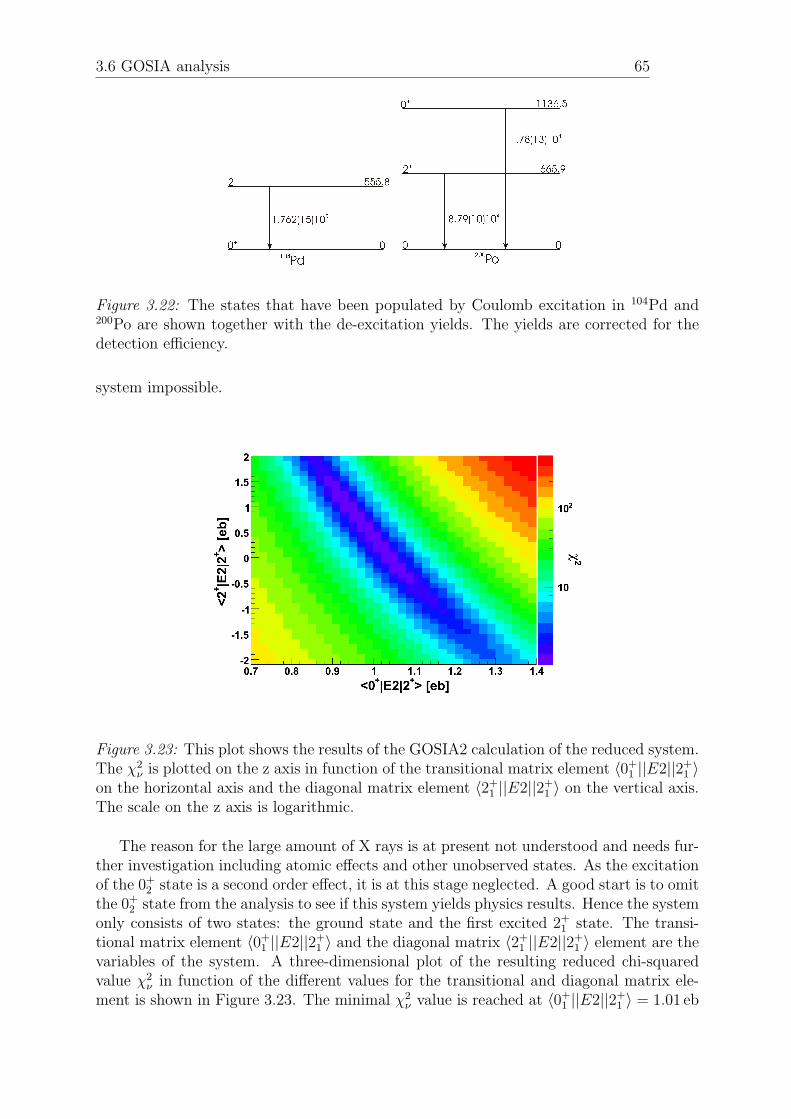
3.6 GOSIA analysis 65

Figure 3.22: The states that have been populated by Coulomb excitation in 104Pd and200Po are shown together with the de-excitation yields. The yields are corrected for thedetection efficiency.

system impossible.

Figure 3.23: This plot shows the results of the GOSIA2 calculation of the reduced system.The χ2

ν is plotted on the z axis in function of the transitional matrix element 〈0+1 ||E2||2+

1 〉on the horizontal axis and the diagonal matrix element 〈2+

1 ||E2||2+1 〉 on the vertical axis.

The scale on the z axis is logarithmic.

The reason for the large amount of X rays is at present not understood and needs fur-ther investigation including atomic effects and other unobserved states. As the excitationof the 0+

2 state is a second order effect, it is at this stage neglected. A good start is to omitthe 0+

2 state from the analysis to see if this system yields physics results. Hence the systemonly consists of two states: the ground state and the first excited 2+

1 state. The transi-tional matrix element 〈0+

1 ||E2||2+1 〉 and the diagonal matrix 〈2+

1 ||E2||2+1 〉 element are the

variables of the system. A three-dimensional plot of the resulting reduced chi-squaredvalue χ2

ν in function of the different values for the transitional and diagonal matrix ele-ment is shown in Figure 3.23. The minimal χ2

ν value is reached at 〈0+1 ||E2||2+

1 〉 = 1.01 eb

3.7 Discussion 66

and 〈2+1 ||E2||2+

1 〉 = 0.55 eb and equals 1.13. As the number of degrees of freedom in thisexperiment equals 5, χ2

ν and χ2 are related as χ2ν = χ2/5. Hence the minimal χ2 equals

5.65. A 1σ deviation from the obtained matrix elements is achieved when the χ2 has in-creased to χ2 +χ2

ν = 6.78 [Gil08]. The values for the matrix elements with a χ2 below thisvalue are selected and shown in Figure 3.24. This plot is used to obtain 1σ error bars. Ithas to be noticed that these error bars are pessimistic as the plot is in this way interpretedas a square instead of the narrow shape that it actually is. The final results for the matrixelements with the associated 1σ error bars are calculated to be 〈0+

1 ||E2||2+1 〉 = 1.01(7

11) eband 〈2+

1 ||E2||2+1 〉 = 0.55(85

85) eb.

Figure 3.24: This plot shows the results of the GOSIA2 calculation of the reduced system.The χ2

ν is plotted on the z axis in function of the transitional matrix element 〈0+1 ||E2||2+

1 〉on the horizontal axis and the diagonal matrix element 〈2+

1 ||E2||2+1 〉 on the vertical axis.

The scale on the z axis is logarithmic. This plot only shows the results with a χ2 that lieswithin the 1σ confidence level. The extremal matrix elements are used to set the errorbars.

The result for the diagonal matrix element is visualized in Figure 3.25 [Bre10]. Fordifferent values of the diagonal matrix element the transitional matrix element is calcu-lated for the 5 experiments separately. As the transitional matrix element is a physicsobservable, the value that is obtained has to be equal for each of the 5 experiments. Hencethe best value for the diagonal matrix elements is the one where the curve is the mostconstant. This is indeed a value around 0.

3.7 Discussion

The value for the transitional matrix element 〈0+1 ||E2||2+

1 〉 = 1.01(711) eb corresponds to a

B(E2, 2+1 → 0+

1 ) value of 29(46) W.u and to a half life of the 2+

1 state of 3.05(33) ps. TheB(E2, 2+

1 → 0+1 ) value is compared to the previously known B(E2, 2+

1 → 0+1 ) values of

3.7 Discussion 67

Figure 3.25: This graph shows a visualization of the result for the value of the diagonalmatrix element. The transitional matrix element is plotted for the 5 different angularranges for different values for the diagonal matrix element.

the polonium isotopes in Figure 3.26. It can be concluded that the B(E2, 2+1 → 0+

1 ) valuefor 200Po that is deduced in this work fits in the generalized seniority scheme and that200Po is indeed a transitional nucleus. However in order to understand the transition, itis necessary to determine also the B(E2, 2+

1 → 0+1 ) values of the neighboring 196,198,202Po

nuclei.

Figure 3.26: This graph shows the known B(E2, 2+1 → 0+

1 ) values of the polonium isotopesin Weisskopf units in function of the mass number A. The B(E2, 2+

1 → 0+1 ) value for 194Po

is taken from [Gra06], the value for 196Po from [Gra09] and the value for 210Po from [Ell73].

As the B(E2, 2+1 → 0+

1 ) value for 200Po is determined and understood, the second-ordereffect of the quadrupole deformation on the Coulomb excitation cross section can also bediscussed. The value that is deduced for the diagonal matrix element 〈2+

1 ||E2||2+1 〉 = 0.55(85

85) ebis compatible with a vanishing quadrupole moment and hence with spherical symmetry.

Conclusion

The polonium isotopes with two protons outside the Z = 82 shell represent an interestingregion of the nuclear chart. 200Po manifests itself as a transitional nucleus between ageneral-seniority-type regime in the heaviest polonium isotopes and a shape-coexistencecharacter in the lightest polonium isotopes. However, questions remain concerning thetransition between these two modes and the degree of mixing between different configu-rations.

In Coulomb excitation the inelastic scattering of a high-energy projectile on a tar-get nucleus is studied. Low-lying excited states in the projectile or target nucleus canbe populated through the exchange of the virtual photon of the electromagnetic inter-action. The cross section for this Coulomb-excitation process depends in first order onthe B(E2, 0+

1 → 2+1 ) value and in second order on the diagonal matrix element of the

populated excited states. The B(E2, 0+1 → 2+

1 ) value renders a direct measure of thecollectivity of the nucleus. The goal of this work was to extract the B(E2, 0+

1 → 2+1 ) value

and the quadrupole moment of the 2+1 state in 200Po by Coulomb excitation.

At REX-ISOLDE (CERN) a 2.85 MeV/u 200Po beam was produced and made to im-pinge on a 104Pd target. The scattered projectile and target nuclei were detected with adouble-sided silicon-strip detector while the MINIBALL gamma-detector array was usedto detect the de-excitation gamma rays. An absolute efficiency curve for the MINIBALLdetector was extracted using 152Eu, 133Ba and 241Am data.

A Coulomb excitation event consists of the detection of two coincident particles thatare scattered back to back in the center-of-mass frame in the particle detector and thedetection of a gamma ray that is in coincidence with these two particles. In a first stepthese Coulomb-excitation events were selected. Thereafter the corresponding gammaspectrum was corrected for the Doppler shift. This is necessary since the energies of thede-excitation gamma rays are Doppler shifted because they are emitted in flight. Finallythe number of counts in the de-excitation peaks of the projectile and the target nucleiwas extracted from the Doppler-corrected gamma spectra and corrected for the detectionefficiency.

Next to the 2+1 → 0+

1 de-excitation peak a large amount of polonium X rays was ob-served. The possible origins of these X rays were investigated. The majority of the X rayswas presumably emitted in the E0 transition of the 0+

2 state to the ground state. This E0transition is favored tremendously above the 0+

2 → 2+1 transition that was not observed.

This result is consistent with the β+/EC-decay study of 200Po in which only the E0 tran-

68

3.7 Discussion 69

sition was observed [Bij98]. The experimentally obtained information was included inGOSIA, a Coulomb excitation analysis code, to deduce the matrix elements connectingthe low-lying excited states in 200Po. However, no physics results could be extracted fromthe whole system. The calculations are complicated by the tremendous amount of X raysand the non observation of the 0+

2 → 2+1 transition. As a compromise a reduced system

containing only the 0+1 ground state and the 2+

1 state was given as input for GOSIA. Fromthe χ2 minimization the values 〈0+

1 ||E2||2+1 〉 = 1.01(7

11) eb and 〈2+1 ||E2||2+

1 〉 = 0.55(8585) eb

were extracted.

The value for the transitional matrix element 〈0+1 ||E2||2+

1 〉 = 1.01(711) eb corresponds

to a B(E2, 2+1 → 0+

1 ) value of 29(46) W.u and to a half life of the 2+

1 state of 3.05(33) ps. TheB(E2, 2+

1 → 0+1 ) value was compared with previously known B(E2, 2+

1 → 0+1 ) values of

other polonium isotopes. It was concluded that the B(E2, 2+1 → 0+

1 ) value for 200Po fits inthe generalized seniority scheme and that 200Po is indeed a transitional nucleus. Howeverin order to understand the transition, it is necessary to determine also the B(E2, 2+

1 → 0+1 )

values of the neighboring 196,198,202Po nuclei. The value that is deduced for the diagonalmatrix element 〈2+

1 ||E2||2+1 〉 = 0.55(85

85) eb is compatible with a vanishing quadrupolemoment and hence with spherical symmetry.

The analysis of this experiment needs to be finalized by looking for a way to extractinformation on the 〈2+

1 ||E2||0+2 〉 matrix element. Also the influence of adding the 0+

2

state to the GOSIA calculations on the already deduced matrix elements 〈0+1 ||E2||2+

1 〉 and〈2+

1 ||E2||2+1 〉 needs to be investigated. The Coulomb-excitation study will be extended to

198,202Po. This experiment is actually part of an experimental campaign studying Coulombexcitation of 198,200,202Po. The remaining beam time (20 shifts) will be scheduled in 2011.The extracted B(E2, 0+

1 → 2+1 ) values can then eventually be compared with theory.

Bibliography

[Alb91] D. Alber et al. Zeitschrift fur Physik A, 339 (1991) 225.

[Ald75] K. Alder and A. Winther. Electromagnetic excitation. North-Holland PublishingCompany, 1975.

[And00] A. N. Andreyev et al. Nature, 405 (2000) 430.

[Bea01] Introduction To Radioactive Nuclear Beams. http://wwwnsg.nuclear.lu.se/basics/rnbintro.asp, 2001.

[Ber95] L. A. Bernstein et al. Physical Review C, 52 (1995) 621.

[Bij95] N. Bijnens et al. Physical Review Letters, 75 (1995) 4571.

[Bij98] N. Bijnens et al. Physical Review C, 58 (1998) 754.

[Bre06] N. Bree. Coulombexcitatie van 68Ni. Master’s thesis, University of Leuven,Faculteit Wetenschappen, 2006.

[Bre10] N. Bree. PhD thesis work, Katholieke Universiteit Leuven, 2010.

[Cas00] R. F. Casten. Nuclear Structure from a Simple Perspective, Second Edition.Oxford University Press, 2000.

[Chu99] S. Y. F. Chu, L. P. Ekstrom, and R. B. Firestone. WWW Table of RadioactiveIsotopes, http://nucleardata.nuclear.lu.se/nucleardata/toi, 1999.

[Ciz97] J. A. Cizewski and W. Younes. Zeitschrift fur Physik A, 358 (1997) 133.

[Cli86] D. Cline. Annual Review of Nuclear and Particle Science, 36 (1986) 683.

[Coc04] T. E. Cocolios, B. A. Marsh, et al. Nuclear Instruments and Methods in PhysicsResearch, B 266 (2004) 4403.

[Coc10] T. E. Cocolios. Single-particle and collective properties around closed shellsprobed by in-source laser spectroscopy. PhD thesis, University of Leuven, Facul-teit Wetenschappen, 2010.

[Czo08] T. Czosnyka, D. Cline, and C. Y. Wu. Coulomb excitation data analysis codeGOSIA, manual, 2008.

[Dir07] J. Diriken. Coulombexcitatiemetingen van neutronrijke koperisotopen. Master’sthesis, University of Leuven, Faculteit Wetenschappen, 2007.

i

BIBLIOGRAPHY ii

[Dup06] P. Van Duppen. The euroschool lectures on physics with exotic beams, Vol. II.Lecture notes in physics, Springer Verlag, Berlin Heidelberg, 2006.

[Ell73] C. Ellegaard et al. Nuclear Physics A, 206 (1973) 83.

[Fah77] C. Fahlander et al. Nuclear Instruments and Methods, 146 (1977) 329.

[Fir99] R.B. Firestone, V.S. Shirley, C.M. Baglin, S.Y.F. Chu, and J. Zipkin. Table ofIsotopes. John Wiley & Sons, 1999.

[Gil08] G. R. Gilmore. Practical Gamma-ray Spectrometry - 2nd Edition. John Wileyand Sons, 2008.

[Gra06] T. Grahn et al. Physical Review Letters, 97 (2006) 062501.

[Gra08] T. Grahn et al. Nuclear Physics A, 801 (2008) 83.

[Gra09] T. Grahn et al. Physical Review C, 80 (2009) 014323.

[Hab00] D. Habs et al. Hyperfine Interactions, 129 (2000) 43.

[Hel83] O. Helene. Nuclear Instruments and Methods, 212 (1983) 319.

[Hel99] K. Helariutta et al. European Physical Journal A, 6 (1999) 289.

[Hey90] K.L.G. Heyde. The Nuclear Shell Model. Springer-Verlag, 1990.

[Hur06] A. M. Hurst. Low-Energy Projectile Coulomb Excitation of Radioactive 70Se and88KrIonBeams. PhD thesis, University of Liverpool, 2006.

[Jul01] R. Julin et al. Journal of Physics G, 27 (2001) R109.

[Kir94] L. Kirkup. Experimental Methods - An introduction to the analysis and presen-tation of data. John Wiley and Sons, 1994.

[Luo86] M. Luontama et al. Zeitschrift fur Physik A, 324 (1986) 317.

[Maj90] A. Maj et al. Nuclear Physics A, 509 (1990) 413.

[May63] M. G. Mayer. Nobel lecture, 1963.

[May77] F. R. May et al. Physics Letters, 68B (1977) 113.

[Oro99] A. M. Oros et al. Nuclear Physics A, 645 (1999) 107.

[Ost02] A. N. Ostrowski et al. Nuclear Instruments and Methods in Physics Research,A 480 (2002) 448.

[Ram87] S. Raman et al. Atomic Data and Nuclear Data Tables, 36 (1987) 1.

[Ril10] Isolde Rilis. http://isolde.web.cern.ch/ISOLDE/, 2010.

[Smi03] N. A. Smirnova et al. Physical Letters B, 569 (2003) 151.

BIBLIOGRAPHY iii

[vdV03] K. van de Vel. Shape coexistence in neutron-deficient polonium and lead nuclei.PhD thesis, University of Leuven, Faculteit Wetenschappen, 2003.

[vdW06] J. van de Walle. Coulomb excitation of neutron rich Zn isotopes. PhD thesis,University of Leuven, Faculteit Wetenschappen, 2006.

[Wau94] J. Wauters et al. Physical Review Letters, 72 (1994) 1329.

[You95] W. Younes et al. Physical Review C, 52 (1995) R1723.

[Zie10] J. F. Ziegler and J. P. Biersack. SRIM2010 http://www.srim.org, 2010.

coulomb excitation of 200po studied at rex-isolde with the

Documents