Technical Report TR-UNL-CSE-2006-0004, Department of Computer Science and Engineering,University of Nebraska–Lincoln, Lincoln, Nebraska, U.S.A., 12 March 2006

Cost-cognizant Test Case Prioritization

Alexey G. Malishevsky∗ Joseph R. Ruthruff† Gregg Rothermel† Sebastian Elbaum†

Abstract

Test case prioritization techniques schedule test cases for regression testing in an order that increases

their ability to meet some performance goal. One performance goal, rate of fault detection, measures how

quickly faults are detected within the testing process. Previous work has provided a metric, APFD, for

measuring rate of fault detection, and techniques for prioritizing test cases in order to improve APFD.

This metric and these techniques, however, assume that all test case and fault costs are uniform. In

practice, test case and fault costs can vary, and in such cases the previous APFD metric and techniques

designed to improve APFD can be unsatisfactory. This paper presents a new metric for assessing the

rate of fault detection of prioritized test cases, APFDC, that incorporates varying test case and fault

costs. The paper also describes adjustments to previous prioritization techniques that allow them, too,

to be “cognizant” of these varying costs. These techniques enable practitioners to perform a new type

of prioritization: cost-cognizant test case prioritization. Finally, the results of a formative case study

are presented. This study was designed to investigate the cost-cognizant metric and techniques and how

they compare to their non-cost-cognizant counterparts. The study’s results provide insights regarding

the use of cost-cognizant test case prioritization in a variety of real-world settings.

Keywords: test case prioritization, empirical studies, regression testing

1 Introduction

Regression testing is an expensive testing process used to detect regression faults [30]. Regression test suites

are often simply test cases that software engineers have previously developed, and that have been saved so

that they can be used later to perform regression testing.

One approach to regression testing is to simply rerun entire regression test suites; this approach is referred

to as the retest-all approach [25]. The retest-all approach, however, can be expensive in practice: for example,

one industrial collaborator reports that for one of its products of about 20,000 lines of code, the entire test

suite requires seven weeks to run. In such cases, testers may want to order their test cases such that those

with the highest priority, according to some criterion, are run earlier than those with lower priority.

Test case prioritization techniques [9, 10, 11, 39, 40, 44] schedule test cases in an order that increases

their effectiveness at meeting some performance goal. For example, test cases might be scheduled in an order

that achieves code coverage as quickly as possible, exercises features in order of frequency of use, or reflects

their historically observed abilities to detect faults.

∗Institute for Applied System Analysis, National Technical University of Ukraine “KPI”, Kiev, Ukraine, malishal@cse.unl.edu†Department of Computer Science and Engineering, University of Nebraska–Lincoln, Lincoln, Nebraska, U.S.A., {ruthruff,

grother, elbaum}@cse.unl.edu

1

One potential goal of test case prioritization is to increase a test suite’s rate of fault detection — that

is, how quickly that test suite tends to detect faults during the testing process. An increased rate of fault

detection during testing provides earlier feedback on the system under test, allowing debugging to begin

earlier, and supporting faster strategic decisions about release schedules. Further, an improved rate of fault

detection can increase the likelihood that if the testing period is cut short, test cases that offer the greatest

fault detection ability in the available testing time will have been executed.

Previous work [9, 11, 39, 40] has provided a metric, APFD, that measures the average cumulative

percentage of faults detected over the course of executing the test cases in a test suite in a given order. This

work showed how the APFD metric can be used to quantify and compare the rates of fault detection of

test suites. Several techniques for prioritizing test cases to improve APFD during regression testing were

presented, and the effectiveness of these techniques was empirically evaluated. This evaluation indicated

that several of the techniques can improve APFD, and that this improvement can occur even for the least

sophisticated (and least expensive) techniques.

Although successful in application to the class of regression testing scenarios for which they were designed,

the APFD metric and techniques rely on the assumption that test case and fault costs are uniform. In

practice, however, test case and fault costs can vary widely. For example, a test case that requires one hour

to fully execute may (all other things being equal) be considered more expensive than a test case requiring

only one minute to execute. Similarly, a fault that blocks system execution may (all other things being

equal) be considered much more costly than a simple cosmetic fault. In these settings, as is later shown in

Section 3, the APFD metric can assign inappropriate values to test case orders, and techniques designed to

improve test case orders under that metric can produce unsatisfactory orders.

To address these limitations, this paper presents a new, more general metric for measuring rate of

fault detection. This “cost-cognizant” metric, APFDC , accounts for varying test case and fault costs.

The paper also presents four cost-cognizant prioritization techniques that account for these varying costs.

These techniques, combined with the APFDC metric, allow practitioners to perform cost-cognizant test case

prioritization by prioritizing and evaluating test case orderings in a manner than considers the varying costs

that often occur in testing real-world software systems. Finally, the results of a formative case study are

presented. This study and its results focus on the use of cost-cognizant test case prioritization, and how the

new cost-cognizant techniques compare to their non-cost-cognizant counterparts.

The next section of this paper reviews regression testing, the test case prioritization problem and the

previous APFD metric. Section 3 presents a new cost-cognizant metric and new prioritization techniques.

Section 4 describes the empirical study. Finally, Section 5 concludes and discusses directions for future

research.

2 Background

This section provides additional background on the problem of regression testing modern software systems.

The test case prioritization problem is then briefly discussed, followed by a review of the APFD metric,

which was designed to evaluate the effectiveness of test case prioritization techniques.

2

2.1 Regression Testing

Let P be a program, let P ′ be a modified version of P , and let T be a test suite developed for P . Regression

testing is concerned with validating P ′.

To facilitate regression testing, engineers typically re-use T , but new test cases may also be required to

test new functionality. Both reuse of T and creation of new test cases are important; however, it is test

case reuse that is of concern here, as such reuse typically forms a part of regression testing processes [30].

In particular, researchers have considered four methodologies related to regression testing and test reuse:

retest-all, regression test selection, test suite reduction, and test case prioritization.1

2.1.1 Retest-all

When P is modified, creating P ′, test engineers may simply reuse all non-obsolete test cases in T to test P ′;

this is known as the retest-all technique [25]. (Test cases in T that no longer apply to P ′ are obsolete, and

must be reformulated or discarded [25].) The retest-all technique represents typical current practice [30].

2.1.2 Regression Test Selection

The retest-all technique can be expensive: rerunning all test cases may require an unacceptable amount of

time or human effort. Regression test selection (RTS) techniques (e.g., [2, 6, 15, 26, 36, 43]) use information

about P , P ′, and T to select a subset of T with which to test P ′. (For a survey of RTS techniques, see [35].)

Empirical studies of some of these techniques [6, 16, 34, 37] have shown that they can be cost-effective.

One cost-benefit tradeoff among RTS techniques involves safety and efficiency. Safe RTS techniques (e.g.,

[6, 36, 43]) guarantee that, under certain conditions, test cases not selected could not have exposed faults in

P ′ [35]. Achieving safety, however, may require inclusion of a larger number of test cases than can be run

in available testing time. Non-safe RTS techniques (e.g., [15, 17, 26]) sacrifice safety for efficiency, selecting

test cases that, in some sense, are more useful than those excluded.

2.1.3 Test Suite Reduction

As P evolves, new test cases may be added to T to validate new functionality. Over time, T grows, and its

test cases may become redundant in terms of code or functionality exercised. Test suite reduction techniques

[5, 18, 21, 29] address this problem by using information about P and T to permanently remove redundant

test cases from T , rendering later reuse of T more efficient. Test suite reduction thus differs from regression

test selection in that the latter does not permanently remove test cases from T , but simply “screens” those

test cases for use on a specific version P ′ of P , retaining unused test cases for use on future releases. Test

suite reduction analyses are also typically accomplished (unlike regression test selection) independent of P ′.

By reducing test-suite size, test-suite reduction techniques reduce the costs of executing, validating, and

managing test suites over future releases of the software. A potential drawback of test-suite reduction, how-

1There are also several other sub-problems related to the regression testing effort, including the problems of automatingtesting activities, managing testing-related artifacts, identifying obsolete tests, elucidating appropriate cost models, and pro-viding test oracle support [20, 25, 27, 30]. These problems are not directly considered here, but ultimately, their considerationwill be important for a full understanding of the costs and benefits of specific techniques within specific processes.

3

ever, is that removal of test cases from a test suite may damage that test suite’s fault-detecting capabilities.

Some studies [45] have shown that test-suite reduction can produce substantial savings at little cost to fault-

detection effectiveness. Other studies [38] have shown that test suite reduction can significantly reduce the

fault-detection effectiveness of test suites.

2.1.4 Test Case Prioritization

Test case prioritization techniques [8, 11, 21, 40, 42, 44], schedule test cases so that those with the highest

priority, according to some criterion, are executed earlier in the regression testing process than lower priority

test cases. For example, testers might wish to schedule test cases in an order that achieves code coverage at

the fastest rate possible, exercises features in order of expected frequency of use, or increases the likelihood of

detecting faults early in testing. A potential advantage of these techniques is that unlike test case reduction

and non-safe regression test selection techniques, they do not discard tests.

Empirical results [11, 40, 44] suggest that several simple prioritization techniques can significantly im-

prove one testing performance goal; namely, the rate at which test suites detect faults. An improved rate of

fault detection during regression testing provides earlier feedback on the system under test and lets software

engineers begin addressing faults earlier than might otherwise be possible. These results also suggest, how-

ever, that the relative cost-effectiveness of prioritization techniques varies across workloads (programs, test

suites, and types of modifications).

Many different prioritization techniques have been proposed [10, 11, 40, 42, 44], but the techniques most

prevalent in literature and practice involve those that utilize simple code coverage information, and those that

supplement coverage information with details on where code has been modified. In particular, techniques

that focus on coverage of code not yet covered have been most often successful. Such an approach has been

found efficient on extremely large systems at Microsoft [42], but the relative effectiveness of the approaches

has been shown to vary with several factors [12].

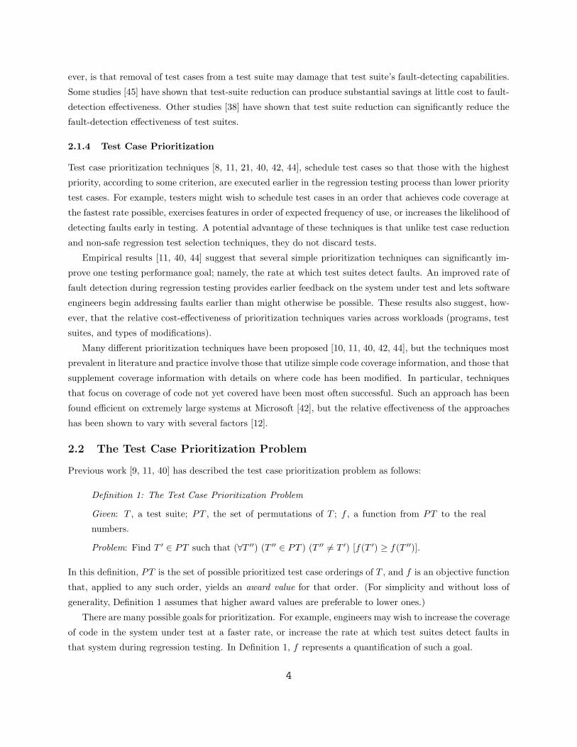
2.2 The Test Case Prioritization Problem

Previous work [9, 11, 40] has described the test case prioritization problem as follows:

Definition 1: The Test Case Prioritization Problem

Given: T , a test suite; PT , the set of permutations of T ; f , a function from PT to the real

numbers.

Problem: Find T ′ ∈ PT such that (∀T ′′) (T ′′ ∈ PT ) (T ′′ 6= T ′) [f(T ′) ≥ f(T ′′)].

In this definition, PT is the set of possible prioritized test case orderings of T , and f is an objective function

that, applied to any such order, yields an award value for that order. (For simplicity and without loss of

generality, Definition 1 assumes that higher award values are preferable to lower ones.)

There are many possible goals for prioritization. For example, engineers may wish to increase the coverage

of code in the system under test at a faster rate, or increase the rate at which test suites detect faults in

that system during regression testing. In Definition 1, f represents a quantification of such a goal.

4

Given any prioritization goal, various test case prioritization techniques may be used to meet that goal.

For example, to increase the rate of fault detection of test suites, engineers might prioritize test cases in terms

of the extent to which they execute modules that have tended to fail in the past. Alternatively, engineers

might prioritize test cases in terms of their increasing cost-per-coverage of code components, or in terms of

their increasing cost-per-coverage of features listed in a requirements specification. In any case, the intent

behind the choice of a prioritization technique is to increase the likelihood that the prioritized test suite can

better meet the goal than would an ad hoc or random order of test cases.

Researchers generally distinguish two varieties of test case prioritization: general and version-specific.

With general prioritization, given program P and test suite T , engineers prioritize the test cases in T with

the aim of finding an order of test cases that will be useful over a succession of subsequent modified versions

of P . With version-specific test case prioritization, given P and T , engineers prioritize the test cases in T

with the aim of finding an order that will be useful on a specific version P ′ of P . In the former case, the

hope is that the prioritized suite will be more successful than the original suite at meeting the goal of the

prioritization on average over subsequent releases; in the latter case, the hope is that the prioritized suite

will be more effective than the original suite at meeting the goal of the prioritization for P ′ in particular.

Finally, although this paper focus on prioritization for regression testing, prioritization can also be em-

ployed in the initial testing of software [1]. An important difference between these applications, however, is

that in regression testing, prioritization techniques can use information gathered in previous runs of existing

test cases to prioritize test cases for subsequent runs; such information is not available during initial testing.

2.3 Measuring Effectiveness

To measure how rapidly a prioritized test suite detects faults (the rate of fault detection of the test suite),

an appropriate objective function is required. (In terms of Definition 1, this measure plays the role of the

objective function f .) For this purpose, a metric, APFD, was previous defined [9, 11, 39, 40] to represent

the weighted “Average of the Percentage of Faults Detected” during the execution of the test suite. APFD

values range from 0 to 100; higher values imply faster (better) fault detection rates.

Consider an example program with 10 faults and a suite of five test cases, A through E, with fault

detecting abilities as shown in Table 1. Suppose the test cases are placed in order A–B–C–D–E to form

a prioritized test suite T1. Figure 1.A shows the percentage of detected faults versus the fraction of T1

used.2 After running test case A, two of the 10 faults are detected; thus 20% of the faults have been

detected after 20% of T1 has been used. After running test case B, two more faults are detected and thus

40% of the faults have been detected after 40% of the test suite has been used. In Figure 1.A, the area

inside the inscribed rectangles (dashed boxes) represents the weighted percentage of faults detected over the

corresponding percentage of the test suite. The solid lines connecting the corners of the rectangles delimit the

area representing the gain in percentage of detected faults. The area under the curve represents the weighted

average of the percentage of faults detected over the life of the test suite. This area is the prioritized test

suite’s average percentage faults detected metric (APFD); the APFD is 50% in this example.

2The use of normalized measures (percentage of faults detected and percentage of test suite executed) supports comparisonsamong test suites that have varying sizes and varying fault detection ability.

5

Test Fault1 2 3 4 5 6 7 8 9 10

A X XB X XC X X X X X X XD XE X X X

Table 1: Example test suite and faults exposed.

A. APFD for prioritized suite T1 B. APFD for prioritized suite T2 C. APFD for prioritized suite T3

0

10

20

30

40

50

60

70

80

90

100

Test Case Order: C−E−B−A−D

0

10

20

30

40

50

60

70

80

90

Test Case Order: E−D−C−B−A

100

0

APFD = 84%APFD = 64%10

20

30

40

50

60

70

80

90

100

0

0

Test Case Order: A−B−C−D−E

APFD = 50%

Percentage of Test Suite Executed Percentage of Test Suite Executed Percentage of Test Suite Executed

Perc

enta

ge o

f Fa

ults

Det

ecte

d

Perc

enta

ge o

f Fa

ults

Det

ecte

d

Perc

enta

ge o

f Fa

ults

Det

ecte

d

20 40 60 80 100 20 40 8080 60 10060 100 20 400

Figure 1: Example test case orderings illustrating the APFD metric.

Figure 1.B reflects what happens when the order of test cases is changed to E–D–C–B–A, yielding

a “faster detecting” suite than T1 with an APFD value of 64%. Figure 1.C shows the effects of using a

prioritized test suite T3 whose test case order is C–E–B–A–D. By inspection, it is clear that this order

results in the earliest detection of the most faults and is an optimal order, with an APFD value of 84%.

For a formulaic presentation of the APFD metric, let T be a test suite containing n sequential test cases,

and let F be a set of m faults revealed by T . Let T ′ be an ordering of T . Let TFi be the first test case in

T ′ that reveals fault i. The APFD for T ′ is:

APFD = 1 − TF1+TF2+...+TFm

nm+ 1

2n(1)

3 A New Approach to Test Case Prioritization

The APFD metric relies on two assumptions: (1) all faults have equal costs (hereafter referred to as fault

severities), and (2) all test cases have equal costs (hereafter referred to as test costs). These assumptions

are manifested in the fact that the metric plots the percentage of faults detected against the percentage of

the test suite run. Previous empirical results [11, 40] suggest that when these assumptions hold, the metric

operates well. In practice, however, there are cases in which these assumptions do not hold: cases in which

faults vary in severity and test cases vary in cost. In such cases, the APFD metric can provide unsatisfactory

results, necessitating a new approach to test case prioritization that is “cognizant” of these varying test costs

and fault severities.

6

This section first describes four simple examples illustrating the limitations of the APFD metric in

settings with varying test costs and fault severities. A new metric is then presented for evaluating test case

orderings that considers varying test costs and fault severities. This presentation is followed by a discussion

of how test costs and fault severities might be estimated by engineers in their own testing settings, and how

to relate such costs and severities to real software. Finally, four techniques that incorporate these varying

costs when prioritizing test cases are presented.

3.1 Limitations of the APFD Metric

Using the testing scenario illustrated earlier in Table 1, consider the following four scenarios of cases in which

the assumptions of equal test costs and fault severities are not met.

Example 1. Under the APFD metric, when all ten faults are equally severe and all five test cases are

equally costly, orders A–B–C–D–E and B–A–C–D–E are equivalent in terms of rate of fault detection;

swapping A and B alters the rate at which particular faults are detected, but not the overall rates of fault

detection. This equivalence would be reflected in equivalent APFD graphs (as in Figure 1.A) and equivalent

APFD values (50%). Suppose, however, that B is twice as costly as A, requiring two hours to execute where

A requires one.3 In terms of faults-detected-per-hour, test case order A–B–C–D–E is preferable to order

B–A–C–D–E, resulting in faster detection of faults. The APFD metric, however, does not distinguish

between the two orders.

Example 2. Suppose that all five test cases have equivalent costs, and suppose that faults 2–10 have

severity k, while fault 1 has severity 2k. In this case, test case A detects this more severe fault along with

one less severe fault, whereas test case B detects only two less severe faults. In terms of fault-severity-

detected, test case order A–B–C–D–E is preferable to order B–A–C–D–E. Again, the APFD graphs and

values would not distinguish between these two orders.

Example 3. Examples 1 and 2 provide scenarios in which the APFD metric proclaims two test case

orders equivalent when intuition says they are not. It is also possible, when test costs or fault severities

differ, for the APFD metric to assign a higher value to a test case order that would be considered less

valuable. Suppose that all ten faults are equally severe, and that test cases A, B, D, and E each require

one hour to execute, but test case C requires ten hours. Consider test case order C–E–B–A–D. Under the

APFD metric, this order is assigned an APFD value of 84% (see Figure 1.C). Consider alternative test case

order E–C–B–A–D. This order is illustrated with respect to the APFD metric in Figure 2; because that

metric does not differentiate test cases in terms of relative costs, all vertical bars in the graph (representing

individual test cases) have the same width. The APFD for this order is 76% — lower than the APFD for

test case order C–E–B–A–D. However, in terms of faults-detected-per-hour, the second order (E–C–B–A–

D) is preferable: it detects 3 faults in the first hour, and remains better in terms of faults-detected-per-hour

than the first order up through the end of execution of the second test case. An analogous example can be

created by varying fault severities while holding test costs uniform.

3These examples frame costs in terms of time for simplicity; Section 3.3 discusses other cost measures.

7

0

0

10

20

30

40

50

60

70

80

90

100

Test Case Order: E−C−B−A−D

APFD = 76%

Percentage of Test Suite Executed

Perc

enta

ge o

f Fa

ults

Det

ecte

d

1008020 40 60

Figure 2: APFD for Example 3.

Example 4. Finally, consider an example in which both fault severities and test costs vary. Suppose

that test case B is twice as costly as test case A, requiring two hours to execute where A requires one.

In this case, in Example 1, assuming that all ten faults were equally severe, test case order A–B–C–D–E

was preferable. However, if the faults detected by B are more costly than the faults detected by A, order

B–A–C–D–E may be preferable. For example, suppose test case A has cost “1”, and test case B has cost

“2”. If faults 1 and 5 (the faults detected by A) are assigned severity “1”, and faults 6 and 7 (the faults

detected by B) are assigned severities greater than “2”, then order B–A–C–D–E achieves greater “units-of-

fault-severity-detected-per-unit-test-cost” than does order A–B–C–D–E.4 Again, the APFD metric would

not make this distinction.

The foregoing examples suggest that, when considering the relative merits of test cases and the relative

severities of faults, a measure for rate-of-fault-detection that assumes that test costs and fault severities are

uniform can produce unsatisfactory results.

3.2 A New Cost-cognizant Metric

The notion that a tradeoff exists between the costs of testing and the costs of leaving undetected faults in

software is fundamental in practice [3, 22], and testers face and make decisions about this tradeoff frequently.

It is thus appropriate that this tradeoff be considered when prioritizing test cases, and so a metric for

evaluating test case orders should accommodate the factors underlying this tradeoff. This paper’s thesis

is that such a metric should reward test case orders proportionally to their rate of “units-of-fault-severity-

detected-per-unit-of-test-cost”.

4This example assumes, for simplicity, that a “unit” of fault severity is equivalent to a “unit” of test cost. Clearly, in practice,the relationship between fault severities and test costs will vary among applications, and quantifying this relationship may benon-trivial. This is discussed further in the following sections.

8

This paper presents such a metric by adapting the APFD metric; the new “cost-cognizant” metric is

named APFDC . In terms of the graphs used in Figures 1 and 2, the creation of this new metric entails

two modifications. First, instead of letting the horizontal axis denote “Percentage of Test Suite Executed”,

the horizontal axis denotes “Percentage Total Test Case Cost Incurred”. Now, each test case in the test

suite is represented by an interval along the horizontal axis, with length proportional to the percentage of

total test suite cost accounted for by that test case. Second, instead of letting the vertical axis in such a

graph denote “Percentage of Faults Detected”, the vertical axis denotes “Percentage Total Fault Severity

Detected”. Now, each fault detected by the test suite is represented by an interval along the vertical axis,

with height proportional to the percentage of total fault severity for which that fault accounts.5

In this context, the “cost” of a test case and the “severity” of a fault can be interpreted and measured

in various ways. If time (for test execution, setup, and validation) is the primary component of test cost, or

if other cost factors such as human time are tracked adequately by test execution time, then execution time

can suffice to measure that cost. However, practitioners could also assign test costs based on factors such as

hardware costs or engineers’ salaries.

Similarly, fault severity could be measured strictly in terms of the time required to locate and correct a

fault, or practitioners could factor in the costs of lost business, litigation, damage to persons or property,

future maintenance, and so forth. In any case, the APFDC metric supports these interpretations. Note,

however, that in the context of the APFDC metric, the concern is not with predicting these costs, which

may be difficult, but with using a measurement of each cost after it has occurred in order to evaluate various

test case orders.

Issues pertaining to the prediction and measurement of test costs and fault severities are discussed in

Sections 3.3 and 3.4, respectively.

Under this new interpretation, in graphs such as those just discussed, a test case’s contribution is

“weighted” along the horizontal dimension in terms of the cost of the test case, and along the vertical

dimension in terms of the severity of the faults it reveals. In such graphs, the curve delimits increased

areas as test case orders exhibit increased “units-of-fault-severity-detected-per-unit-of-test-cost”; the area

delimited constitutes the new APFDC metric.

To illustrate the APFDC metric from this graphical point of view, Figure 3 presents graphs for each of

the four scenarios presented, using Table 1, in the preceding subsection. The leftmost pair of graphs (Figure

3.A) correspond to Example 1: the upper of the pair represents the APFDC for test case order A–B–C–D–

E, and the lower represents the APFDC for order B–A–C–D–E. Note that whereas the (original) APFD

metric did not distinguish the two orders, the APFDC metric gives preference to order A–B–C–D–E,

which detects more units of fault severity with fewer units of test cost at an early stage in testing than does

order B–A–C–D–E.

The other pairs of graphs illustrate the application of the APFDC metric in Examples 2, 3, and 4. The

pair of graphs in Figure 3.B, corresponding to Example 2, show how the new metric gives a higher award to

5As in the original metric, the use of normalized metrics (relative to total test suite cost and total fault severity) for test costsand fault severities supports meaningful comparisons across test suites of different total test costs and fault sets of differentoverall severities.

9

00

10

10

20

20

30

30

40

40

50

50

60

60

70

70

80

80

90

90

100

100

Area = 46.67%

Test Case Order A-B-C-D-E

Percentage Total Test Case Cost Incurred

Perc

enta

ge T

otal

Fau

lt Se

veri

ty D

etec

ted

00

10

10

20

20

30

30

40

40

50

50

60

60

70

70

80

80

90

90

100

100

Area = 43.33%

Test Case Order B-A-C-D-E

A. APFDs corresponding to Example 1

Percentage Total Test Case Cost Incurred

Perc

enta

ge T

otal

Fau

lt Se

veri

ty D

etec

ted

00

10

10

20

20

30

30

40

40

50

50

60

60

70

70

80

80

90

90

100

100

Area = 53.64%

Test Case Order A-B-C-D-E

Percentage Total Test Case Cost IncurredPe

rcen

tage

Tot

al F

ault

Seve

rity

Det

ecte

d

00

10

10

20

20

30

30

40

40

50

50

60

60

70

70

80

80

90

90

100

100

Area = 51.82%

Test Case Order B-A-C-D-E

B. APFDs corresponding to Example 2

Percentage Total Test Case Cost Incurred

Perc

enta

ge T

otal

Fau

lt Se

veri

ty D

etec

ted

00

10

10

20

20

30

30

40

40

50

50

60

60

70

70

80

80

90

90

100

100

Area = 52.50%

Test Case Order C-E-B-A-D

Percentage Total Test Case Cost Incurred

Perc

enta

ge T

otal

Fau

lt Se

veri

ty D

etec

ted

00

10

10

20

20

30

30

40

40

50

50

60

60

70

70

80

80

90

90

100

100

Area = 68.93%

Test Case Order E-C-B-A-D

C. APFDs corresponding to Example 3

Percentage Total Test Case Cost IncurredPe

rcen

tage

Tot

al F

ault

Seve

rity

Det

ecte

d

00

10

10

20

20

30

30

40

40

50

50

60

60

70

70

80

80

90

90

100

100

Area = 52.38%

Test Case Order A-B-C-D-E

Percentage Total Test Case Cost Incurred

Perc

enta

ge T

otal

Fau

lt Se

veri

ty D

etec

ted

00

10

10

20

20

30

30

40

40

50

50

60

60

70

70

80

80

90

90

100

100

Area = 54.76%

Test Case Order B-A-C-D-E

D. APFDs corresponding to Example 4

Percentage Total Test Case Cost Incurred

Perc

enta

ge T

otal

Fau

lt Se

veri

ty D

etec

ted

Figure 3: Examples illustrating the APFDC metric.

the test case order that reveals the more severe fault earlier (A–B–C–D–E), under the assumption that the

severity value assigned to each of faults 2–10 is 1 and the severity value assigned to fault 1 is 2. The pair of

graphs in Figure 3.C, corresponding to Example 3, show how the new metric distinguishes test case orders

involving a high-cost test case C: instead of undervaluing order E–C–B–A–D, the metric now assigns it

greater value than order C–E–B–A–D. Finally, the pair of graphs in Figure 3.D, corresponding to Example

4, show how the new metric distinguishes between test case orders when both test costs and fault severities

are non-uniform, under the assumptions that test case B has cost 2 while each other test case has cost 1, and

that faults 6 and 7 each have severity 3 while each other fault has severity 1. In this case, the new metric

assigns a greater value to order B–A–C–D–E than to order A–B–C–D–E.

The APFDC metric can be quantitatively described as follows. (Here, the formula for APFDC is

given; its derivation is presented in Appendix A.) Let T be a test suite containing n test cases with costs

t1, t2, . . . , tn. Let F be a set of m faults revealed by T , and let f1, f2, . . . , fm be the severities of those faults.

Let TFi be the first test case in an ordering T ′ of T that reveals fault i. The (cost-cognizant) weighted

average percentage of faults detected during the execution of test suite T ′ is given by the equation:

APFDC =

∑m

i=1 (fi × (∑n

j=TFitj −

12 tTFi

))∑n

j=1 tj ×∑m

i=1 fi

(2)

10

If all test costs are identical and all fault costs are identical (∀i ti = t and ∀i fi = f), this formula

simplifies as follows:

∑m

i=1 (f × (∑n

j=TFit − t 1

2 ))

n × m × t × f=

∑m

i=1 (n − TFi + 1 − 12 )

nm=

1 −TF1 + TF2 + · · · + TFm

nm+

1

2n

Thus, Equation 2 remains applicable when either test costs or fault severities are identical, and when both

test case costs and fault severities are identical, the formula reduces to the formula for APFD.

3.3 Estimating Test Costs

Cost-cognizant prioritization requires estimates of the costs of executing test cases. There are two issues

connected with test cost: estimating it for use in prioritizing test cases, and measuring or estimating it for

use in assessing an order in terms of APFDC .

The cost of a test case is related to the resources required to execute and validate it. Various objective

measures are possible. For example, when the primary required resource is machine or human time, test

cost can be measured in terms of the actual time needed to execute a test case. Another measure considers

the monetary costs of test case execution and validation; this may reflect amortized hardware cost, wages,

cost of materials required for testing, earnings lost due to delays in failing to meet target release dates, and

so on [3, 22].

Some test cost estimates can be relatively easy to obtain for use in APFDC computation, which occurs

after test suite execution. For example, a practitioner can simply time each test case, or quantify the

resources each test case required. Cost estimation is more difficult to perform before testing starts; however,

it is necessary if the practitioner wishes to consider costs in prioritization. In this case, practitioners need to

predict test costs. One approach for doing this is to consider the functionalities of the software likely to be

invoked by a test case, and estimate the expense of invoking those functionalities. For example, a test case

that exercises the file input and output capabilities of the software might be expected to be more expensive

than a test case that exercises erroneous command-line options. Another approach, and the one that is used

in the case study described in Section 4, is to rely on test cost data gathered during a preceding testing

session. Under this approach, one assumes that test costs do not change significantly from one release to

another. Alternatively, one might adjust estimates based on predictions of the effects of modifications.

Note that the APFDC metric is not dependent on the approach used to obtain test costs. The metric

requires only a quantification of the expense of running each test case, regardless of what that quantification

specifically measures (e.g., time, wages, materials, etc.) or how that quantification is obtained (e.g., an

assessment made during previous testing). This allows the metric to be applicable to the many types of

testing processes that occur in practice.

11

3.4 Estimating Fault Severities

Cost-cognizant prioritization also requires an estimate of the severity of each fault that can be revealed by

a test case. As with test cost, with fault severity there are two issues: estimating it for use in prioritizing

test cases, and measuring or estimating it for use in assessing an order in terms of APFDC .

The severity of a fault reflects the costs or resources required if a fault (1) persists in, and influences, the

users of the software after it is released; or (2) does not reach users, yet affects the organization or developers

due to factors such as debugging time. Once again, various measures of fault severity are possible. For

example:

• One measure considers the severity of a fault in terms of the amount of money expended due to the

fault. This approach could apply to systems for which faults can cause disastrous outcomes resulting

in destruction of property, litigation costs, and so forth.

• A second measure considers a fault’s effects on the cost of debugging. This approach could apply to

systems for which the debugging process can involve many hours of labor or other resources such as

hardware costs or material costs.

• A third measure considers a fault’s effects on software reliability. This approach could apply to systems

for which faults result in inconvenience to users, and where a single failure is not likely to have safety-

critical effects (e.g., office productivity software). In this case, the main effect involves decreased

reliability which could result in loss of customers.

• Other measures could combine the three just described. For example, one could measure a fault’s

severity based on both the money expended due to the fault and the loss of customers due to the

perception of decreased software reliability.

As with test costs, practitioners would be concerned with both before- and after-the-fact fault severity

estimation. When testing is complete, practitioners have information about faults and can estimate their

severities to use in APFDC computation. (Of course, this is not as easy as with test cost, but it is routine

in practice, for example, when classifying faults to prioritize maintenance activities.) On the other hand,

before testing begins, practitioners need to estimate the severity of potential faults as related to their system

or tests so that this information can be used by prioritization techniques, and this is far more difficult than

with test cost. To be precise, practitioners require a metric on test cases that quantifies the severity of the

faults that each test case reveals.

If practitioners knew in advance the faults revealed by a given test case, and knew their severities,

associating test cases with severities would be trivial. In practice, however, this information is not available

before testing is completed. Two possible estimation approaches, however, involve assessing module criticality

and test criticality [7]. Module criticality assigns fault severity based on the importance of the module (or

some other code component such as a block, function, file, or object) in which a fault may occur, while test

criticality is assigned directly to test cases based on an estimate of the importance of the test, or the severity

of the faults each test case may detect.

12

Section 4 examines a measure of test criticality that is derived from the importance of the operations

being executed by each test case. In practice, the test cases in a test suite execute one or more system

functionalities or operations. In this scenario, the criticality of each test case is a function of the importance

of each operation executed by the test case. Also note that operations vary across systems, and may need

to be considered at different granularities depending on the nature of the system under testing. The idea

behind this measurement is that faults exposed in an operation that is of high importance to the system

would likely be more severe than those faults exposed in an operation that is less important.

3.5 Using Scales to Assign Test Costs and Fault Severities

For some systems, the approaches suggested earlier, taken alone, may not quantify test costs and fault

severities in a manner that relates sufficiently to the characteristics of the software system under test. The

following two scenarios describe cases in which this might happen, and suggest how practitioners may go

about better quantifying test costs and fault severities in such cases.

Scenario 1. In some systems, the importance of fault severities can greatly outweigh the importance of test

case costs. For example, in some safety-critical systems, any fault can have potentially serious consequences,

and the cost of the test cases used to detect these faults might be inconsequential in comparison to the

importance of detecting these faults. In these cases, practitioners might want to adjust their measures of

test costs and fault severities so that fault severities have substantially greater influence on prioritization

than test costs.

Scenario 2. In some systems, the cost of certain test cases may be much higher than those of other

test cases and some faults may be much more severe than other faults, and the test cost and fault severity

estimation approaches described earlier may not satisfactorily capture these characteristics. For example,

practitioners often classify faults into categories such as “cosmetic” and “critical”. Again, in these cases,

practitioners might want to adjust the costs and severities assigned to each test case and each fault.

Two strategies can be used in practice to adjust test costs and fault severities: weighting and bucketing.

Practitioners can use weightings to exaggerate or understate the importance of certain tests or faults, to

address situations such as Scenario 1. For example, practitioners can increase the severity measures of

the most expensive faults (or the cost measures of the most expensive test cases) so that they are further

separated from other, less expensive, faults (or test cases).

Bucketing groups test costs or fault severities into equivalence classes so that they share the same quan-

tification. Practitioners can use bucketing to group particular types of test cases and faults, or to group

test cases and faults that they consider to be similar according to some criterion, to address situations such

as Scenario 2 (e.g., [41, 31]). For example, practitioners often have a limited number of classes used to

rank faults such as “Cosmetic”, “Moderate”, “Severe”, and “Critical”, and bucketing is one mechanism for

distributing faults into these classes.

The case study described in Section 4 investigates the use of several combinations of weighting and

bucketing to adjust and group test costs and fault severities.

13

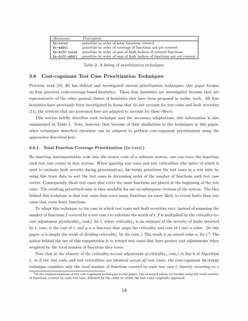
Mnemonic Description

fn-total prioritize in order of total functions covered

fn-addtl prioritize in order of coverage of functions not yet covered

fn-diff-total prioritize in order of sum of fault indices of covered functions

fn-diff-addtl prioritize in order of sum of fault indices of functions not yet covered

Table 2: A listing of prioritization techniques.

3.6 Cost-cognizant Test Case Prioritization Techniques

Previous work [10, 39] has defined and investigated various prioritization techniques; this paper focuses

on four practical code-coverage-based heuristics. These four heuristics are investigated because they are

representative of the other general classes of heuristics that have been proposed in earlier work. All four

heuristics have previously been investigated in forms that do not account for test costs and fault severities

[11]; the versions that are presented here are adapted to account for these effects.

This section briefly describes each technique and the necessary adaptations; this information is also

summarized in Table 2. Note, however, that because of their similarities to the techniques in this paper,

other techniques described elsewhere can be adapted to perform cost-cognizant prioritization using the

approaches described here.

3.6.1 Total Function Coverage Prioritization (fn-total)

By inserting instrumentation code into the source code of a software system, one can trace the functions

each test case covers in that system. When ignoring test costs and test criticalities (the latter of which is

used to estimate fault severity during prioritization), fn-total prioritizes the test cases in a test suite by

using this trace data to sort the test cases in decreasing order of the number of functions each test case

covers. Consequently, those test cases that cover the most functions are placed at the beginning of the test

suite. The resulting prioritized suite is then available for use on subsequent versions of the system. The idea

behind this technique is that test cases that cover many functions are more likely to reveal faults than test

cases that cover fewer functions.

To adapt this technique to the case in which test costs and fault severities vary, instead of summing the

number of functions f covered by a test case t to calculate the worth of t, f is multiplied by the criticality-to-

cost adjustment g(criticalityt, costt) for t, where criticalityt is an estimate of the severity of faults detected

by t, costt is the cost of t, and g is a function that maps the criticality and cost of t into a value. (In this

paper, g is simply the result of dividing criticalityt by the costt.) The result is an award value at for t.6 The

notion behind the use of this computation is to reward test cases that have greater cost adjustments when

weighted by the total number of functions they cover.

Note that in the absence of the criticality-to-cost adjustment g(criticalityt, costt) in line 6 of Algorithm

1, or if the test costs and test criticalities are identical across all test cases, the cost-cognizant fn-total

technique considers only the total number of functions covered by each test case t, thereby reverting to a

6In the implementations of the cost-cognizant techniques in this paper, ties in award values are broken using the total numberof functions covered by each test case, followed by the order in which the test cases originally appeared.

14

Algorithm 1 Cost-cognizant total function coverage prioritization.

Input: Test suite T , function trace history TH , test criticalities Tcrit, and test costs Tcost

Output: Prioritized test suite T ′

1: begin2: set T ′ empty3: for each test case t ∈ T do4: calculate number of functions f covered by t using TH

5: calculate award value at of t as f ∗ g(criticalityt, costt) using Tcrit and Tcost

6: end for7: sort T in descending order based on the award value of each test case8: let T ′ be T

9: end

non-cost-cognizant technique.7 (This is true of the three cost-cognizant techniques presented later in this

section as well.)

Algorithm 1 describes the process for performing total function coverage prioritization. In this algorithm,

trace history TH is the data structure that records information regarding the coverage achieved by each test

case; in total function coverage prioritization, this data structure records the functions covered by each test

case. The data structure Tcrit contains the criticality of each test case, and the data structure Tcost contains

the cost of each test case.

The time complexity of total function coverage prioritization is analyzed as follows. Assume the size of

test suite T is n, and the number of functions in the system is m. The time required in line 4 to calculate

the total number of covered functions for one test case t is O(m) because all m functions must be checked

against t in TH . (The cost of deciding whether a function is covered by a specific test case is constant

once TH is loaded.) Because function coverage must be decided for all n test cases, the time complexity

of calculating cost-cognizant coverage information in lines 3–6 is O(n · m). (Again, the cost of deciding the

criticality and cost of each test case is constant once Tcrit and Tcost are loaded.) The time required in line

7 to sort the test suite is O(n log n) using an appropriate algorithm. Therefore, the overall time complexity

is O(n · m + n logn).

Note that the algorithms introduced in other work that perform analogous forms of total coverage prior-

itization, such as total statement coverage prioritization, are similar to Algorithm 1. Using total statement

coverage prioritization as an example, in the previous analysis, m would represent the number of statements

in the system, and the TH data structure would record information regarding the statements covered by

each test case. Although such modifications would not change the formal complexity of the algorithm, in

practice, performance could be impacted by choice of type of coverage.

3.6.2 Additional Function Coverage Prioritization (fn-addtl)

Additional function coverage prioritization greedily selects a test case that yields the greatest function

coverage of the system, then adjusts the coverage data about each unselected test case to indicate its

coverage of functions not yet covered. This process is repeated until all functions have been covered by at

7In fact, the fn-total technique reverts to the technique described in earlier work [11].

15

Algorithm 2 Cost-cognizant additional function coverage prioritization.

Input: Test suite T , function trace history TH , test criticalities Tcrit, test costs Tcost

Output: Prioritized test suite T ′

1: begin2: set T ′ empty3: initialize values of vector Vcov as “uncovered”4: while T is not empty do5: for each test case t ∈ T do6: calculate number of functions fa additionally covered by t using TH and Vcov

7: calculate award value at of t as fa ∗ g(criticalityt, costt) using Tcrit and Tcost

8: end for9: select test t with the greatest award value

10: append t to T ′

11: update Vcov based on the functions covered by t

12: if no more coverage can be added then13: reset Vcov

14: end if15: remove t from T

16: end while17: end

least one test case. When all functions have been covered, remaining test cases must also be prioritized; one

way to do this is by (recursively) resetting all functions to “not covered” and reapplying additional function

coverage prioritization on the remaining test cases. The idea behind this technique is that test cases that

cover many functions that have not been previously covered are more likely to reveal faults not revealed by

previous tests.

To adapt this technique to the case in which test costs and fault severities vary, instead of summing the

number of functions covered additionally by a test case t to calculate the worth of t, the number of functions

fa additionally covered by t is multiplied by the criticality-to-cost adjustment g(criticalityt, costt) for t, where

criticalityt, costt, and g have definitions similar to those used in total function coverage prioritization. The

notion behind the use of this computation is to reward test cases that have greater cost adjustments when

weighted by the additional functions they cover.

Algorithm 2 describes the process for performing additional function coverage prioritization. In this

algorithm, TH , Tcrit, and Tcost have definitions similar to those in total function coverage prioritization.

Vcov is a vector of values “covered” or “uncovered” for each function in the system. The vector records the

functions that have been covered by previously selected test cases.8

The time complexity of additional function coverage prioritization is analyzed as follows. Assume that

the size of test suite T is n, and the number of functions in the system is m. The time required in line 6

in Algorithm 2 to calculate the additional function coverage for one test case is O(m). (As in total function

coverage prioritization, the cost of deciding function coverage, as well as querying test criticalities and test

costs, is constant once the appropriate data structures have been loaded.) Therefore, the cost of lines 5–8 is

8Note that, in the additional function coverage prioritization algorithm, when Vcov reaches full coverage, this means that allfunctions covered by T have been covered, not that all functions in the system have been covered, because there is no guarantee(or requirement) that T covers every function in the system.

16

O(n · m). In line 9, the time required to select the test case with the greatest award value from the n test

cases is O(n). The cost of adding covered functions to Vcov in line 11 is O(m) in the worst-case. Detecting

when no more coverage can be added to Vcov in line 12 takes constant time with an appropriate base of

information. This brings the cost of the entire while loop to O(n · m + n + m) = O(n · m). The whole loop

itself executes n times. Therefore, the overall time complexity of the algorithm is O(n2 · m).

As with total function coverage prioritization, the additional function coverage prioritization algorithm

could be modified to accommodate other types of coverage without changing the algorithm’s formal com-

plexity, although in practice performance could be affected.

3.6.3 Total Function Difference-based Prioritization (fn-diff-total)

Certain functions are more likely to contain faults than others, and this fault proneness can be associated

with measurable software attributes [4, 13, 24]. One type of test case prioritization that has not yet dis-

cussed in this paper takes advantage of this association by prioritizing test cases based on their coverage of

functions that are likely to contain faults. Given such a representation of fault proneness, a form of test case

prioritization based on function coverage would assign award values to test cases based on their coverage of

functions that are likely to contain faults.

Some representations of fault proneness have been explored in earlier studies [13, 28]. This represented

fault proneness based on textual differences in source code using the Unix diff tool. This metric, whose

values are termed change indices in this paper, works by noticing the functions in the program that have been

modified between two versions of a software system. This is done by observing, for each function present in

a version v1 and a subsequent version v2, whether a line was inserted, deleted, or changed, in the output of

the Unix diff command when applied to v1 and v2. (This work uses a binary version of the diff metric

that assigns a “1” to functions that had been modified between versions, and a “0” to functions that did not

change between versions.) The intuition behind this metric is that functions that have been changed between

two versions of a system are more likely to contain faults than functions that have not been changed.

To adapt this technique to the case in which test costs and fault severities vary, instead of summing

change index values for each function f covered by a test case t, the values of cif × g(criticalityt, costt)

are summed for each f covered by t, where cif is the change index of f , and criticalityt, costt, and g have

definitions similar to those provided earlier. The notion behind this computation is to reward test cases that

have greater cost adjustments when weighted by the number of total changed functions that they cover.

Algorithm 3 describes the process for performing total function difference-based prioritization. This

algorithm is similar to that of total function coverage prioritization. TH , Tcrit, and Tcost have definitions

similar to those used earlier. CI is a record of the change index values corresponding to each function in the

system.

The time complexity of total function difference-based prioritization is analyzed as follows. Assume the

size of test suite T is n, and the number of functions in the system is m. If T contains n test cases, the time

required in line 5 to calculate the functions covered by a test case t is O(m), and the time required in lines

6–8 to sum the award values for the covered functions is also O(m) in the worst case. Therefore, the time

17

Algorithm 3 Cost-cognizant total function difference-based prioritization.

Input: Test suite T , function trace history TH , function change indices CI , test criticalities Tcrit, test costsTcost

Output: Prioritized test suite T ′

1: begin2: set T ′ empty3: for each test case t ∈ T do4: set at of t to zero5: calculate set of functions F covered by t using TH

6: for each function f ∈ F do7: increment award value at by cif × g(criticalityt, costt) using CI , Tcrit, and Tcost

8: end for9: end for

10: sort T in descending order based on the award values of each test case11: let T ′ be T

12: end

required in lines 3–9 to calculate the award values for all n test cases is O(n · 2m) = O(n · m). (As before,

the cost of calculating function coverage, as well as the costs of querying change indices, test criticalities,

and test costs, are constant once the appropriate data structures are loaded.) The time required in line 10

to sort the test suite is O(n log n) using an appropriate algorithm. Therefore, the overall time complexity is

O(n · m + n log n).

Although this time complexity is equivalent to the complexity of total function coverage prioritization,

note that total function difference-based prioritization requires the computation of a change index for each

function before prioritization — a cost that is not incurred in total function coverage prioritization. Therefore,

total function difference-based prioritization is likely to be more expensive that total function coverage

prioritization in practice. (Even if such information is already available through a mechanism such as

version control, processing this information is still required of total function difference-based prioritization.)

Algorithm 3 can also be modified to support a different type of coverage without changing the algo-

rithm’s formal complexity, although the type of coverage used is likely to impact performance in practice.

Note, however, that acquiring change index information for some levels of coverage, such as statement-level

coverage, is generally more difficult than for function-level coverage.

3.6.4 Additional Function Difference-based Prioritization (fn-diff-addtl)

Additional function difference-based prioritization is similar to additional function coverage prioritization.

During execution, the algorithm maintains information listing those functions that are covered by at least

one test case in the current test suite. When adding a new test case t to the test suite, for each test case

in the test suite, the algorithm computes the sum of the change indices for each function f covered by t,

except those functions that have already been covered by at least one test case in the current test suite. The

test case with the highest sum of these change indices is then the next test case added to the prioritized suite.

18

Furthermore, just as with the additional function coverage prioritization technique, when no more coverage

can be added, each function’s coverage is reset and the remaining test cases are then added to the test suite.

To adapt this technique to the case in which test costs and fault severities vary, instead of summing

change index values for each function f covered by a test case t, the values of cif × g(criticalityt, costt) are

summed for each f covered additionally by t, where cif , criticalityj, costj, and g have definitions similar

to those provided earlier. The notion behind the use of this computation is to reward test cases that have

greater cost adjustments when weighted by the number of additional changed functions that they cover.

The time complexity of the additional function difference-based prioritization algorithm, which is given

in Algorithm 4, is analyzed as follows. Assume that the size of test suite T is n, and the number of functions

in the system is m. In lines 6–10, all m functions will be additionally covered by all n test cases in the

worst-case. Thus, the time required in lines 5–11 to calculate the award values for all n test cases is O(n ·m).

In line 12, the time required to select the test case with the greatest award value is O(n). The cost of adding

covered functions to Vcov in line 14 is O(m) in the worst-case. This brings the cost of the entire while loop

to O(n ·m +n + m) = O(n ·m). Because the while loop executes n times, the overall time complexity of the

algorithm is O(n2 · m).

Once again, note that although this complexity is equivalent to that of additional function coverage

prioritization, additional function difference-based prioritization requires that change indices be computed

before prioritization occurs. Also as before, Algorithm 4 could be modified to support a different level

Algorithm 4 Cost-cognizant additional function difference-based prioritization.

Input: Test suite T , function trace history TH , function change indices CI , test criticalities Tcrit, test costsTcost

Output: Prioritized test suite T ′

1: begin2: set T ′ empty3: initialize values of vector Vcov as “uncovered”4: while T is not empty do5: for each test case t ∈ T do6: set at of t to zero7: calculate set of functions F additionally covered by t using TH and Vcov

8: for each function f ∈ F do9: increment award value at by cif × g(criticalityt, costt) using CI , Tcrit, and Tcost

10: end for11: end for12: select test t with the greatest award value13: append t to T ′

14: update Vcov based on the functions covered by t

15: if no more coverage can be added then16: reset Vcov

17: end if18: remove t from T

19: end while20: end

19

of coverage without changing the algorithm’s formal complexity, although the algorithm’s performance in

practice is likely to be affected.

4 A Formative Case Study

Cost-cognizant prioritization is a new way of approaching the Test Case Prioritization Problem. As such,

there has been little study into using this approach in practical testing settings.

To investigate the application of the cost-cognizant APFDC metric and the previously presented four

techniques in testing real-world software systems, as well as some of the ramifications of using them, a

formative case study was conducted. Case studies [23, 46] can help researchers and practitioners assess

the benefits of using a new technique, such as cost-cognizant test case prioritization, by investigating the

technique’s effects on a single system or a small number of systems that are not chosen at random and

are not selected to provide the levels of replication that would be expected of a formal experiment. Case

studies have the benefit of exposing the effects of a technique in a typical situation, but such studies do

not generalize to every possible situation because they do not seek to investigate a case representing every

possible situation [23].

The goal of this formative case study is not to make summative judgments regarding the four cost-

cognizant techniques or the APFDC metric. Further, because of limitations of the object of study (such as

the varying number of faults in each version) that is described later in this section, it may not be appropriate

to draw such summative judgments in this case study.

Instead, formative insights into the operation of cost-cognizant prioritization are gleaned from the appli-

cation of the cost-cognizant techniques to a real-world software system. In particular, this study observes

the operation of the techniques and metric using a real-world software system, and notes how test case order-

ings created using cost-cognizant prioritization compare in effectiveness (in terms of the APFDC metric) to

orderings created using non-cost-cognizant prioritization. The study considers some specific results in detail

in order to better understand how the techniques operate.

In the upcoming subsections, the setting in which the case study was conducted is presented. The design

of the study, and how it seeks to meet the aforementioned goals, is described. Finally, the study’s results

are presented and discussed.

4.1 Study Setting

To use a cost-cognizant prioritization technique to order the test cases in a software system’s test suite, a

few things are required:

1. a version of the software system to test,

2. a test suite with which to test that version,

3. a criticality associated with each test case in the test suite, and

4. a cost associated with each test case.

20

In addition, to analyze the fault detection capabilities of the prioritized test suite (in this case, using the

APFDC metric), one also requires:

5. a set of faults in the version of the system that is being tested, and

6. a severity associated with each fault.

The following subsections reflect the steps undertaken in this case study to facilitate the application

of this paper’s cost-cognizant prioritization techniques by obtaining or creating the foregoing items, and

the subsequent calculation of APFDC values in order to evaluate the fault detection capabilities of test

case orderings. First, a software system was selected to study. Second, a number of tasks were completed

to prepare this object of study for analysis. Concurrently, various tools were implemented and utilized to

prioritize the test cases of the test suite, measure various attributes of the software system, and complete

the APFDC calculations. This section first describes the software system selected to be the object of study,

and then describes the steps undertaken to complete the previously mentioned tasks.

4.1.1 Selecting an Object of Study

As an object of study the software system Empire [14] was selected. Empire is a non-trivial, open-source,

client-server software system programmed in the C programming language. Empire is a system that was

partially organized for use in empirical studies in previous work [33].

Empire is a strategic game of world domination between multiple human players. Each player begins the

game as the “ruler” of a country. Throughout the game, the players acquire resources, develop technology,

build armies, and engage in diplomacy with other players in an effort to conquer the world. Either defeating

or acquiring a concession from all opposing players achieves victory. In addition to the players, each game of

Empire has one or more “deities” who install and maintain the game on a host server. As might be expected,

certain actions are reserved only for deities.

The Empire software system is divided into a server and a client, which are named emp-server and

emp-client, respectively. After the initialization of emp-server on the host server by the deities, the game

progresses with the players and deities using emp-client to connect and issue commands, which correspond

to their desired actions, to emp-server. The emp-server processes each command issued by an emp-client

and returns the appropriate output. This case study was conducted using nine versions of the emp-server

portion of Empire.

There are several reasons for selecting emp-server as a test subject. First, emp-server is a relatively

large system (approximately 63,000 to 64,000 lines of non-blank, uncommented source code), has had an

active user-base for over 15 years, and has had 21 releases just in the last seven years. Second, emp-server is

written in the C programming language, thereby providing compatibility with existing analysis tools. Third,

because Empire is distributed under the GNU General Public License Agreement, it is available at no cost.

Fourth, as described in Section 4.1.3, operational profiles for the system were required, and collecting such

profiles for Empire is feasible. Finally, previous studies [33] have created a specification-based test suite for

emp-server, and the four prioritization techniques can be applied to this suite. The emp-server test suite,

21

created by the category partition method [32], is of a fine granularity, meaning the individual test cases in

the test suite each exercise individual units of functionality independently. This test suite contains 1985 test

cases, and represents a test suite that might be created by engineers in practice if they were doing functional

testing.

4.1.2 Inserting and Detecting Regression Faults

To measure the rate of fault detection of prioritized test suites, the APFDC values of test suites are based on

how quickly suites’ tests detect faults. Consequently, to determine whether a test case detects faults, the case

study must be designed such that the test suite is attempting to detect known faults. Clearly, in practice,

the faults in a software system are not known in advance during the regression testing process. However, by

designing a case study in which the detection of known faults in the test subject is attempted, cost-cognizant

test case prioritization can be empirically examined and address the study’s research questions.

The question, then, is what known faults should be measured. While Empire comes with extensive docu-

mentation concerning the commands available to users, it does not have adequate documentation describing

the known faults in each version of the software system. Furthermore, for reasons that will soon be described,

it is important to have the ability to toggle faults on and off, meaning, for each faulty section of code, an

alternative section is required that is not faulty. One could attempt to locate faults distributed with each

emp-server version, but that would require an implemented resolution to each fault. This is not a desirable

strategy because, without the intricate knowledge of the system that is possessed by the developers, one

risks unknowingly creating additional faults in the system.

Consequently, a strategy of inserting seeded faults into the software system was selected. A seeded fault

is a fault that is intentionally introduced into a software system, usually for the sole purpose of measuring

the effectiveness of a test suite.

To introduce seeded faults into the software system, several graduate students with at least two years

of C programming experience, and no knowledge of the study, were asked to introduce several faults into

each version of emp-server. These students used their programming knowledge to insert faults in areas of

code in which a software engineer might accidentally introduce a fault in practice. Furthermore, because

the focus of this work is the detection of regression faults, the areas of code in which a student could insert

a fault were limited to those that were modified in the preceding version of the test subject. Each student,

after identifying a section of code in which to introduce a fault, made a copy of that section of code and

surrounded each section by preprocessor statements that, depending on the definition of certain variables,

toggles on either the faulty or the non-faulty code. This process was completed for all nine versions of

emp-server.

Following the precedent set by previous studies [10, 11, 40], this case study was not based on faults

that were either impossible or too easy to detect, as the former are not the target of test case prioritiza-

tion and the latter are likely to be detected by developers prior to the system testing phase that this paper

is concerned with. Therefore, all initially seeded faults that were detected either by more than 20% of the test

22

cases in the test suite, or by no test cases at all, were excluded. This resulted in between one and nine seeded

faults per emp-server version.

To calculate the rate of fault detection of each prioritized test suite for each version of emp-server, it

must be known whether each test case in the suite reveals any of the faults that were seeded in each version.

To address this need, for each version of emp-server, a fault matrix was gathered that documents the faults

(if any) each test case reveals in that version. The fault matrix is used both to calculate the severity of each

seeded fault (described in Section 4.1.3), and to assist in the APFDC calculations for each prioritized test

suite.

To gather a fault matrix for each version, numerous runs of the test suite were executed where the test

cases were unordered. In the initial run of the test suite, all seeded faults were turned off, and the output

of each test case was recorded into an output file. A sequence of test suite runs was then executed. In the

first run of this sequence, the first seeded fault was toggled on, and the remainder of the faults were toggled

off. By recording and comparing the output of each test case during this test suite run with the output

of the initial (unordered) test suite run, it was determined whether that test case revealed the first seeded

fault. Repeating this process for the other seeded faults yielded the necessary information to complete a

fault matrix for this version of the test subject.

While conducting this process, it was noticed that due to various nondeterministic issues in running

Empire, such as a bad transmission from the emp-client to the emp-server, a command will occasionally

(approximately once per thousand test case executions) fail for no apparent reason. Consequently, for each

version, an additional set of runs of the test suite were executed, repeating the process outlined above, to

gather a second fault matrix. By performing a logical and operation between the two fault matrices for each

version, only those faults that were revealed in both sets of test suite runs were kept, thereby substantially

reducing the possibility of erroneously recording a revealed fault due to a nondeterministic issue.

4.1.3 Calculating Fault Severity

As discussed in Section 3.4, there are various methods for calculating the severity of a fault. This case study

based a fault’s severity upon the likelihood that a user might encounter that fault during his or her use of a

system. But how does one measure the likelihood of encountering faults during the usage of emp-server?

Software systems provide various operations that users utilize to complete the task for which the system

was designed. For example, some of the operations of a word-processing software system may be text

insertion, text deletion, and saving, creating, and opening a document. Likewise, Empire consists of a

number of operations that allow players and deities to participate in an Empire game. These operations

come in the form of commands the players and deities issue to emp-server. Examples of some Empire

operations include fire, announce, move, and update. Using the documentation provided with the system,

182 operations were identified in the base Empire version. The operations of the software system that are

executed by each test case in a test suite were documented using an operation matrix.

One strategy that might be utilized by software engineers when testing a software system involves gath-

ering an operational profile for that system. An operational profile records, for each operation, the frequency

23

with which that operation is likely to be utilized by a user. This frequency is usually relative to all other

operations. Using the preceding example, in a word-processing system, the “text insertion” operation may

be utilized 85% of the time, the “text deletion” operation 10% of the time, the “save document” operation

2% of the time, the “create document” operation 1% of the time, the “open document” operation 1% of the

time and the “print document” operation 1% of the time. By indicating each operation’s frequency of use,

operational profiles enable software engineers to make decisions regarding the testing of a software system.

For example, engineers may focus their testing on operations that users utilize at least 5% of the time.

Additionally, engineers may decide that a fault in an operation that a user frequently utilizes is more severe

than a fault in an operation that a user rarely utilizes, regardless of that fault’s impact on the execution of

the system. This latter method is the intuition behind this study’s fault severity measurements.

An operational profile for the case study was collected by running an Empire game with three experienced

players, all of whom responded to a game announcement posted on the Empire newsgroup. The source code

of emp-server was modified to record the commands issued by each player.9 At the completion of the game,

the number of times each command was issued by the players was determined. By dividing this number

by the total number of commands issued in the game, an operational profile was created estimating each

command’s frequency of use. To explain later metrics, for each operation i, this frequency is defined as the

importance of operation i.

To calculate the severity of each fault in a version of the test subject, begin with the operation matrix

and the fault matrix for that version. By using the fault matrix, which maps faults to various test cases,

and the operation matrix, which maps each test case to an operation, various operations are associated with

each fault. Next, using the operational profile, sum the importance of each operation that is associated with

a fault. This sum is the severity assigned to each seeded fault in a version of the test subject. Note that

these severities are used only in the APFDC calculations to evaluate test case orderings, as test criticality

is used to estimate fault severities during the prioritization process.

4.1.4 Calculating Test Case Criticality

As discussed in Section 3.4, test case criticalities are used as a metric to quantify the severity of the faults

that each test case reveals. However, it is not possible to predict the faults, if any, revealed by each test

case during prioritization — before test cases are executed. This study’s test criticality metric, which must

therefore be derived without knowledge of what faults each test case might expose, is meant to estimate the

potential severity of faults that might be uncovered by a test case.

In this study, test case criticality is derived from the operational profile and the operation matrix. The

operations executed by a test case were determined by referring to the operation matrix. Each test case’s

criticality is measured as the importance of the operation it executes, as determined from the operational

profile. The notion behind this measure is that faults in operations of high importance are more severe than

faults in operations of low importance.

9The players of the Empire game were not informed that their usage was being monitored, as that might have altered theirbehavior; however, all data was collected in such a manner that the anonymity of the commands issued by each player waspreserved.

24

4.1.5 Calculating Test Cost

Section 3.3 discussed how engineers can use a variety of criteria to measure test costs. This case study

measures each test case’s cost by summing the amount of time required, in seconds, to execute that test

case and validate that test case’s output by comparing it against expected output (from a previous run). To

gather this timing data, two runs of the test suite were completed on non-instrumented executables. During

each run, standard UNIX system calls were used to record the time at the beginning and end of each test

case’s execution, and at the beginning and end of the process to determine whether each test case revealed

any faults in the software system. After completing these two runs of the test suite, the cost of each test case

run was calculated by averaging the results from the two runs. This average is the metric used to represent

the cost of each test case in the suite.

4.1.6 Obtaining Coverage and Difference Information

For the fn-total and fn-addtl prioritization techniques, the functions executed by each test case are traced

by inserting instrumentation code into the original source code of the software system. The Aristotle

program analysis system [19] is used to insert instrumentation code into emp-server and generate test

coverage information.

The fn-diff-total and fn-diff-addtl techniques require a representation of the fault proneness of

each function. Change indices are one representation of fault proneness that observe the functions that

have been modified between a baseline version and a modified version of a software system. As described in

Section 3.6.3, the change indices for each version of emp-server were created using the Unix diff utility.

4.2 Design

4.2.1 Test Cost and Fault Severity Scales

As discussed in Sections 3.3 and 3.4, in practice there are many ways that engineers assign test costs and

fault severities. In particular, engineers often give test costs and fault severities various weightings, and

group those costs and severities into buckets.

To investigate the cost-cognizant metric and prioritization techniques using these approaches, scales were

used to assign costs and severities to test cases and faults, and in some cases to group those assigned values.

(Because test criticalities were used to estimate fault severity during prioritization, scales operated on test

costs and test criticalities in that setting.) Four scales were selected. The first scale — the unit scale —

does not assign varying test costs or fault severities, while the other three scales are inspired by practical

scenarios.

Unit Scale: The first scale does not discriminate between the costs of test cases; rather, the costs

of all test cases are uniform. This non-cost-cognizant scale corresponds to the case in which test

costs (or fault severities) are ignored. Using this scale for both test costs and test criticalities has

the effect of rendering the four techniques non-cost-cognizant.

25

Original Scale: This scale assigns to each test case (or fault) the actual cost or criticality (or

severity) that was computed for it using the approaches described in Sections 4.1.3–4.1.5.10

Bucketed Linear Scale: In this scale, the values from the original scale are sorted and split evenly

into buckets. The cost used for each test case (or severity for each fault) corresponds to its

bucket number.11 Using this approach, the buckets are used to group test cases and faults, and

the bucket numbers are used to assign weights to those groupings. This linear distribution is

similar to that used in the Mozilla application.12

Bucketed Exponential Scale: This scale is similar to the bucketed linear scale, except that it uses

an exponential scale to assign weights by assigning to each test case a cost (or fault a severity)

of (bn − 1), where b is the base of the scale and n is the linear bucket number; in this study,

b = 2. This scale was devised as an alternative to the bucketed linear scale by using weights to

exaggerate the cost of the most expensive test cases and the severity of the worst faults.

This paper does not claim that these four scales are the only scales that engineers could consider. These

scales were chosen with real-world applications in mind; however, in this study, they are used only as a

means for creating varying settings of test costs and fault severities. In spite of this, engineers might find

scales such as these to be useful in testing their own systems. Also, because there has been little research

into cost-cognizant test case prioritization, these scales might inspire other engineers and researchers to

investigate other approaches.

4.2.2 Variables

Each unit of analysis was created by varying the test costs and fault severities of an emp-server version.

All four prioritization techniques were then separately used to prioritize the emp-server test suite. As such,

there were two independent variables: (1) a selection of test cost and fault severity scales, of which there

are 16 possible combinations; and (2) one of four cost-cognizant prioritization techniques from Section 3.6.

Each resulting prioritized test suite was then assessed using the APFDC metric described in Section 3.2.

This metric was the dependent variable in this study.

4.2.3 Procedures

All 16 possible scale combinations were used to prioritize the test suite for each emp-server version. The rate

of fault detection of each resulting test case ordering was then evaluated according to the APFDC metric.

The first scale — unit test costs and unit test criticalities — represents a non-cost-cognizant prioritization

scheme, while the other 15 combinations represent varying possibilities for cost-cognizant prioritization.

10For all four scales, in the case of test criticalities and fault severities, this assignment was done by altering the operationalprofile using these scales, and then generating test criticalities and fault severities from this altered operational profile.

11All values that were originally zero were assigned to the first “zero” bucket.12This distribution was obtained by querying the “bugzilla” database [31] for “Resolved” bugs on the Netscape Browser for

PC-windows 2000. For more information on Mozilla, see http://www.mozilla.org. For more information on Mozilla testingand fault recording, see http://bugzilla.mozilla.org.

26

To examine whether cost-cognizant prioritization generally provided test case orderings with greater

rates of fault detection than non-cost-cognizant prioritization, this study began by considering comparisons

between cost-cognizant techniques and non-cost-cognizant techniques. In this context, the APFDC metric

was used to measure the rate of fault detection of the test case ordering resulting from each technique in

order to make comparisons.

To consider some specific results in detail, post-mortem qualitative analyses were performed; specific

comparisons between cost-cognizant techniques and non-cost-cognizant techniques were considered in detail

in order to discern the reasons why one form of prioritization performed better than the other. This type

of comparison was performed in order to analyze how cost-cognizant techniques would have performed had

varying test costs and fault severities not been used (i.e., if the non-cost-cognizant technique would have

been used), and vice versa.

4.3 Limitations

Like any empirical study, this study has several limitations that should be considered when interpreting its

results; pertinent limitations are discussed here.

This study was conducted using only a single test suite. Unfortunately, while multiple test suites would

have been ideal, the test suite utilized in this study required several weeks to create, rendering the production

of further test suites infeasible given the time frame allotted to this study. The study also examines output

only at the end of test cases, assumes that this output can be categorized as either “pass” or “fail”, and

assumes that all reported errors are due to faults in the source and not in the test cases.

The quantitative function used to measure rate of fault detection, APFDC , has two limitations. First,

APFDC does not reward a test case for detecting a fault that has been previously detected. Such test

cases, however, might prove useful to software engineers in practice. In this study, the fine granularity of

the test cases in the test suite helps mitigate this factor because each test case exercises a single operation.

However, the APFDC metric itself is still limited because a test suite with a coarser granularity may be

quite susceptible to this issue. Second, APFDC does not consider the analysis time required to prioritize

the test cases of a test suite. Previous work [40], however, suggests that analysis time is small in comparison

to test suite execution time, or that analysis can be performed before the critical regression testing process

begins.

Empire is a software system where the operational profile gathered is highly dependent on the type of

game being played, and there are many types of games possible. Still, it is possible that the profile gathered

for this study’s game is not representative of those for general Empire games. Finally, the fault seeding

process described in Section 4.1.2 allowed for the “activation” of one fault at a time, therefore preventing

one seeded fault from masking the effects of another. However, although the fault seeders were instructed to

insert faults that mimic those that they have seen in their own programming experience, the faults seeded

in emp-server may differ from the faults and fault patterns that exist in software systems.

27

4.4 Results and Discussion

All possible variations of the four cost-cognizant techniques were first compared, using the four particular

scales for test costs and test criticalities, with their non-cost-cognizant counterparts. Although 16 possible

scale combinations were used to create these cost-cognizant techniques, one scale combination (unit test

costs and unit test criticalities) yields a non-cost-cognizant prioritization technique. Therefore, because the

other 15 combinations use some form of cost-cognizant prioritization, there were 15 possible comparisons

within each technique (i.e., 15 scale combinations to compare to the scale combination of unit test costs and

unit test criticalities). Because four techniques and nine emp-server versions are considered, there are 540

comparisons between cost-cognizant and non-cost-cognizant techniques.

On examining the results of these comparisons, contrary to expectations, in 74.6% of the comparisons

(403 out of 540), the test case orderings resulting from cost-cognizant prioritization had a worse rate of

fault detection, according to the APFDC metric, than their associated non-cost-cognizant orderings. Table

3 depicts these overall results; cells shaded gray show the cases in which the non-cost-cognizant technique

performed better than the specified cost-cognizant technique.

As can be seen in this table, in five versions (v3, v5, v6, v7, and v8), the test case orderings produced

by cost-cognizant techniques almost always had worse rates of fault detection than those produced by the

corresponding non-cost-cognizant techniques. However, in the other four versions (v1, v2, v4, and v9), the

results were relatively even between the two types of prioritization. There did not appear to be any particular

characteristics in these two sets of versions that might account for these findings. For example, the former

set of emp-server versions contained between one and seven seeded faults, while the latter set of versions

contained between one and nine faults. As another example, the former set of versions contained between

32 and 157 modified functions, while the latter set of versions contained between nine and 245 modified

functions.

Despite this, in considering these results as a whole, there do appear to have been many cases in which

cost-cognizant techniques were beneficial to regression testing, although further work is needed to investigate

in detail the types of software systems or versions for which this benefit may occur. Still, these results

are surprising because one might expect cost-cognizant prioritization to be superior to non-cost-cognizant

prioritization the majority of the time.

In examining the individual comparisons between cost-cognizant techniques and non-cost-cognizant tech-

niques, there are many cases where cost-cognizant techniques performed much better than non-cost-cognizant

techniques, and vice versa. Consequently, to determine possible explanations for the aforementioned results,

and to meet the earlier goal of examining individual comparisons between cost-cognizant techniques and non-

cost-cognizant techniques, in Sections 4.4.1–4.4.4 two cases where cost-cognizant prioritization had a greater

rate of fault detection than non-cost-cognizant prioritization are examined in detail, as are two cases where

non-cost-cognizant prioritization had a greater rate of fault detection. Each of these four cases involves a

cost-cognizant technique where either varying test costs or varying test criticalities were used, but not both.

This allows for better isolation of the factor that may have caused the results seen in each case in order to

draw meaningful conclusions. The derived observations are used to discuss the underlying reasons why, for

28

cost scale/crit scale Technique v1 v2 v3 v4 v5 v6 v7 v8 v9

unit/orig fn-total

unit/orig fn-addtl

unit/orig fn-diff-total

unit/orig fn-diff-addtl

unit/buck-lin fn-total

unit/buck-lin fn-addtl

unit/buck-lin fn-diff-total

unit/buck-lin fn-diff-addtl

unit/buck-exp fn-total

unit/buck-exp fn-addtl

unit/buck-exp fn-diff-total

unit/buck-exp fn-diff-addtl

orig/unit fn-total

orig/unit fn-addtl

orig/unit fn-diff-total

orig/unit fn-diff-addtl

orig/orig fn-total

orig/orig fn-addtl

orig/orig fn-diff-total

orig/orig fn-diff-addtl

orig/buck-lin fn-total

orig/buck-lin fn-addtl

orig/buck-lin fn-diff-total

orig/buck-lin fn-diff-addtl

orig/buck-exp fn-total

orig/buck-exp fn-addtl

orig/buck-exp fn-diff-total

orig/buck-exp fn-diff-addtl

buck-lin/unit fn-total

buck-lin/unit fn-addtl

buck-lin/unit fn-diff-total

buck-lin/unit fn-diff-addtl

buck-lin/orig fn-total

buck-lin/orig fn-addtl

buck-lin/orig fn-diff-total

buck-lin/orig fn-diff-addtl

buck-lin/buck-lin fn-total

buck-lin/buck-lin fn-addtl

buck-lin/buck-lin fn-diff-total

buck-lin/buck-lin fn-diff-addtl

buck-lin/buck-exp fn-total

buck-lin/buck-exp fn-addtl

buck-lin/buck-exp fn-diff-total

buck-lin/buck-exp fn-diff-addtl

buck-exp/unit fn-total

buck-exp/unit fn-addtl

buck-exp/unit fn-diff-total

buck-exp/unit fn-diff-addtl

buck-exp/orig fn-total

buck-exp/orig fn-addtl

buck-exp/orig fn-diff-total

buck-exp/orig fn-diff-addtl

buck-exp/buck-lin fn-total

buck-exp/buck-lin fn-addtl

buck-exp/buck-lin fn-diff-total

buck-exp/buck-lin fn-diff-addtl

buck-exp/buck-exp fn-total

buck-exp/buck-exp fn-addtl

buck-exp/buck-exp fn-diff-total

buck-exp/buck-exp fn-diff-addtl

Table 3: An overview of the 540 possible comparisons between cost-cognizant and non-cost-cognizant pri-oritization. The 403 shaded cells mark cases where non-cost-cognizant prioritization was superior to cost-cognizant prioritization.

29

each case, one form of prioritization performed better than the alternative. These insights are summarized

in Section 4.4.5.

4.4.1 Cost-cognizant Prioritization has Greater Rate of Fault Detection: Case #1

In this case, the first version (v1) of emp-server is considered using the fn-addtl technique. Version v1

contains six faults. In the cost-cognizant case, test costs are considered using the unit scale, and test criti-

calities (during prioritization) and fault severities (after testing for APFDC evaluation) using the bucketed

exponential scale. The APFDC of the resulting test case ordering is approximately 97.1. However, if the

fn-addtl technique is considered using non-cost-cognizant prioritization (test costs and test criticalities

using the unit scales), the APFDC of the resulting test case ordering is approximately 91.8.

The cost-cognizant technique provided a greater rate of fault detection according to the APFDC metric

in this particular case. Because the only difference between the two techniques is the use of varying test

criticalities, only the varying test criticality scales could have accounted for the differences in APFDC

between the cost-cognizant and non-cost-cognizant techniques. To explore the underlying reasons for this

difference, the fault detection behavior of the test case orderings resulting from both forms of prioritization

was considered in greater detail.

Examining the behavior of non-cost-cognizant prioritization, test cases were prioritized based only on

the number of functions that are additionally covered by a new test case. The resulting test case ordering

detects its first fault after the fourth test case. However, this fault accounts for only approximately 15.4%

of the total fault severity. The 19th test case detects a second fault accounting for 7.7% of the total fault

severity, and the 91st test case detects a third fault accounting for another 59.6%, bringing the total fault

severity detected to 82.7%. The remaining three faults are detected with the 349th, 366th, and 685th test

cases, respectively.

The improved rate of fault detection in the case of cost-cognizant prioritization can be attributed primarily

to the very beginning of the prioritized test suite; the second test case selected by cost-cognizant prioritization

revealed a fault accounting for approximately 59.6% of the total fault severity. In this case, using the

operational profile, test criticality rightfully assigned the test case a high criticality, which, combined with

the test case’s moderately high function coverage, placed the test ahead of many other non-fault-revealing

tests that would have had higher award values using non-cost-cognizant prioritization. The first fault-

revealing test under non-cost-cognizant prioritization — the fourth test overall in that setting — was still

selected ninth under cost-cognizant prioritization, resulting in another 15.4% of detected fault severity. This

allowed the prioritized test suite to detect 75% of the total fault severity in just nine tests. The remaining

four faults were revealed by the 142nd, 203rd, 381st, and 550th test cases.

The incorporation of feedback by fn-addtl is one reason why cost-cognizant prioritization performed

better than non-cost-cognizant prioritization in this particular case. Recall that fn-addtl chooses test cases

based on the number of functions that are additionally covered by a new test case. In this case, with respect

to non-cost-cognizant prioritization, this had the effect of shutting out a test case that would have detected

approximately 59.6% of the total fault severity until all functions had been covered. However, the use of

30

the test criticality metric increased the award value of this test case so that it was placed before other test

cases that actually covered more as-yet-uncovered functions. This allowed the test case ordering to reveal a

very severe fault that accounted for approximately 59.6% of the total fault severity. Test criticality was an

important addition to test case prioritization in this particular case.

4.4.2 Cost-cognizant Prioritization has Greater Rate of Fault Detection: Scenario #2

In this case, the ninth version (v9) of emp-server is considered using the fn-total technique. Version v9

contains two faults. In the cost-cognizant case, test costs are considered using the bucketed linear scale,

and test criticalities (during prioritization) and fault severities (after testing for APFDC evaluation) using

the unit scale. The APFDC of the resulting test case ordering is approximately 83.1. However, if the

fn-total technique is considered using non-cost-cognizant prioritization, the APFDC of the resulting test

case ordering is 59.9.

The only difference between the two techniques in this case is the use of varying test costs, so only the

varying test cost scales could have accounted for the differences in APFDC between the two techniques. As

before, the fault detection behavior of both test case orderings is considered in greater detail.

In v9, there are two faults of equal severity. Using both forms of prioritization, each fault is detected by

the same two unique test cases (which are placed at different points in the ordered test suite). For simplicity,

these two test cases are referred to as ta and tb. In non-cost-cognizant prioritization using the fn-total

technique, the ordering of test cases is done purely on the basis of the total number of functions covered by

each test case. Test case ta covers 253 functions, while tb covers 181 functions, causing them to be ordered

as the 86th and 1450th test cases, respectively. In this setting, although 50% of the total fault severity is

detected quite early with the 86th test case, the second fault is not detected until over 73% of the test suite

has been executed.

The two fault-exposing test cases, ta and tb, are ordered earlier under cost-cognizant prioritization using

the bucketed linear test cost scale. In this setting, the cost incurred by ta is much lower than that of many

other test cases in the test suite. This causes the award value of ta to increase, and so the test case is ordered

32nd in the test suite. Similarly, the consideration of test costs causes tb to be ordered as the 703rd test case

— 747 test cases earlier than in non-cost-cognizant prioritization. As such, the APFDC of this test case

ordering is much higher.

The use of the linear bucketed scale to assign test costs to test cases: in this particular example, improved

the APFDC value of the test case ordering as compared to non-cost-cognizant prioritization. Using the linear

bucketed scale caused the test costs to be more dispersed than they would have been using the original scale.

(This is seen in Section 4.4.4, which, though a separate example, uses the same test suite and the same original

test costs.) This increased dispersing caused the award values computed by the prioritization technique to

be sensitive to test costs, allowing the technique to make a cost-effectiveness decision by choosing a test case

that is less expensive than other test cases.

31

4.4.3 Non-cost-cognizant Prioritization has Greater Rate of Fault Detection: Case #1

In this case, the fourth version (v4) of emp-server is considered using the fn-total technique. Version

v4 contains six faults. In the cost-cognizant case, test costs are considered using the unit scale, and fault

severities (during APFDC evaluation) using the original scale. (Test criticalities are not considered because

non-cost-cognizant prioritization is used.) The APFDC of the resulting test case ordering is approximately

83.5. However, if the fn-total technique is considered using non-cost-cognizant prioritization, the APFDC

of the resulting test case ordering is approximately 95.6.

In the non-cost-cognizant prioritization test case ordering, the 72nd of the 1985 test cases detects three

of the six faults in v4, and these three faults account for almost 88.5% of the total fault severity in v4. Soon

after, the 192nd test case detects a fourth fault, and in total more than 99.5% of the total fault severity has

been detected at this point. The 675th and 935th test cases detect the remaining two faults.

Now consider the case in which cost-cognizant prioritization is used. Unlike in the non-cost-cognizant

case, in this case fault detection starts much later: at the 223rd test. This test detects about 66.45% of the

total fault severity, but after 11.2% of the test suite has been executed. In contrast, more than 99.5% of the

total fault severity was detected at this point in the non-cost-cognizant case. Returning to the cost-cognizant

case, after executing the 529th test, three more faults are detected, bringing the total fault severity detected

to approximately 99.5%. Finally, the 1152nd and 1167th tests detect the remaining two faults, although

these faults have small fault severity relative to the other faults.

The test case that was ordered 72nd using non-cost-cognizant prioritization was placed early in the test

suite because of its high function coverage; it executes 261 total functions in the emp-server source code.

However, the award value of this test case is greatly diminished using cost-cognizant prioritization because

it has a much lower test criticality than many other test cases. The test criticality of this test case was very

close to zero because, according to the operational profile, most of the system operations that the test case

executes are not used often. This low test criticality caused the test case to be ordered 1237th using the

cost-cognizant fn-total technique. This trend was also observed in relation to many other test cases that

would have detected new faults.

Initially reflecting on this result, one might wonder whether test criticality does not correlate well with

fault severity. Recall that test criticalities were used as a measure of the importance of a test case during

prioritization by attempting to correlate test cases with fault severities, which were used after prioritization

by the APFDC metric. However, because test criticalities were (and after all, must in practice be) derived

without knowledge of the faults exposed by each test case, the metric merely estimates the potential severity

that might be uncovered by a test case. If test criticalities do not correlate well with fault severities, they

may actually hurt prioritization.

An analysis of this particular example, however, found preliminary evidence that this was not the case.

This analysis involved calculating correlation coefficients, which are used to determine the relationship be-

tween two properties (in this case, between various contributors in cost-cognizant prioritization). Correlation

coefficients indicate the strength of the linear association between variables. All computations of correlation

coefficients were performed on this particular case. The computations were based on the 1985 test cases and

32

their associated attributes (award values, test criticalities, etc.) using both cost-cognizant prioritization and

non-cost-cognizant prioritization.

The correlation coefficient between function coverage and the award values used to prioritize test cases

was approximately -0.006, indicating no relationship one way or the other between function coverage and

award values in this particular example. More interesting, however, was that the correlation coefficient

between test criticality and total fault severity in this example was also very low — approximately -0.01 —

once again indicating no relationship one way or the other. This underscores the role of test criticalities in

this particular example, where test criticality estimates did not reflect fault severity, resulting in lower rates

of fault detection.

A second possible reason why this study’s test criticality metric hurt cost-cognizant prioritization in this

particular example may involve how the metric was employed in the criticality-to-cost adjustment g (see

Section 3.6). It is possible that a different adjustment would improve the APFDC of test case orderings in

these and other cases, or even that combining coverage information with a criticality-to-cost adjustment is

inappropriate. Further work that investigates the use of a wider variety of criticality-to-cost adjustments,

and considers different ways to combine these types of adjustments with coverage information, would be

useful to investigate these possibilities.

Of course, the observations derived from this particular example do not necessarily generalize to the

wide variety of situations in which test criticality may be used. Also, test criticality values were assigned

using only one of many possible scales. Finally, this study’s test criticality calculations were dependent on

the operational profile, and this individual profile might have been responsible for the negative role of test

criticality in this example. While further study is necessary to investigate all of these possibilities, this study’s

formative findings point out directions for researchers to explore in determining some of the underlying causes

when cost-cognizant prioritization does not perform as well as its non-cost-cognizant counterpart.

4.4.4 Non-cost-cognizant Prioritization has Greater Rate of Fault Detection: Case #2

In this case, the eighth version (v8) of emp-server is considered using the fn-total technique. Version v8

contains one fault. In the cost-cognizant case, test costs are considered using the original scale and fault

severities using the unit scale. (Test criticalities are not considered because non-cost-cognizant prioritization

is used.) The APFDC of the resulting test case ordering is approximately 73.1. However, if the fn-total

technique is considered using non-cost-cognizant prioritization, the APFDC of the resulting test case ordering

is approximately 78.1.

In v8, the one fault is detected by only two of the 1985 test cases in the test suite. For simplicity, these

test cases are referred to as ta and tb. Using the original scale for assigning test costs, the costs assigned

to ta and tb are approximately 15.6 and 16.2. (Recall from Section 4.1.5 that test costs were measured in

seconds.) Furthermore, the range of test costs for 99.7% of the test cases in the test suite is approximately

[14.5 . . .22.0], with many test costs residing at the lower end of this range. These costs, combined with the

total function coverage of the test cases, cause ta and tb to be assigned as the 538th and 796th test cases,

33

respectively, in the prioritized test suite. However, when test costs are not considered, ta and tb are ordered

427th and 422th, respectively, causing the fault to be detected earlier.

Because the actual test costs were preserved by the original scale and packed into a tight range, there was

not a great deal of difference among the costs of many test cases. This allowed the total function coverage

information used by the fn-total technique to have a strong, positive linear association on the award values

used to prioritize test cases (correlation coefficient of approximately 0.92) in this particular example. Also,

using the original scale, test costs did not have as strong an impact on the award values, as the correlation

coefficient was approximately −0.33. Therefore, there was a small negative correlation in this particular case

between test costs and award values. That is, as test costs tended to go up, award values tended to go down,

and vice versa. (This is not necessarily surprising in this paper’s implementation of fn-total because test

criticalities are divided by test costs in the criticality-to-cost adjustment g.)

These observations indicate that test costs assigned using the original scale — even when they have an

adverse impact on the test case ordering — may not have a large impact on prioritization. In fact, this may

be one reason why the APFDC values calculated for cost-cognizant and non-cost-cognizant prioritization

were much closer in this case than in the previous cases.

Another possible lesson of these observations, however, is that a scale that allows a large number of

test costs (or test criticalities) to migrate into a narrow, common range may be undesirable because it may

no longer appropriately distinguish test costs well enough to support effective cost-cognizant prioritization.

This suggests that scales that use buckets, such as the bucketed linear or bucketed exponential scales, may

be desirable in order disperse the test cost values of the cases in a test suite. However, note that the

aforementioned effect was possible only because the criticality-to-cost adjustment was multiplied into the

total number of functions covered by each test case.

4.4.5 Summary of Insights

The foregoing results and discussion highlight the fact that test case prioritization techniques that account

for test costs and test criticalities can be beneficial, and can be directly responsible for more effective test

case orderings in some cases. However, in other cases, these techniques are not successful. Possible reasons

for both types of observations are now discussed.

In Section 4.4.1, test criticality was the primary reason why an important fault-revealing test case was

prioritized earlier using cost-cognizant prioritization than with non-cost-cognizant prioritization. In contrast,

in Section 4.4.3 test criticality caused a similarly important test case to be prioritized far into the test suite,

resulting in a lower APFDC than that with non-cost-cognizant prioritization.

A preliminary lesson to researchers and practitioners from this study is that test criticality, or whatever

equivalent method is used to estimate the severity of the faults detected by test cases, is very important

to cost-cognizant prioritization (or at least to prioritization schemes using the criticality-to-cost adjustment

approach used by the particular techniques in this paper). These test criticality values should therefore be

calculated and assigned (using scales) with care.

34

In the case of test costs, preliminary evidence in this paper’s study indicates that the distribution of

those costs can impact the performance of a cost-cognizant technique. In Section 4.4.2, the bucketed linear

scale caused the test costs to be dispersed, and in this particular example helped the technique prioritize

more cost-effective test cases towards the beginning of the test suite. On the other hand, in Section 4.4.4

the vast majority of the test cases were tightly grouped together into a narrow range of values, and the

cost-cognizant technique appeared to have difficulty distinguishing test cases using this information.

A preliminary lesson to researchers and practitioners is that, at least in the case of test costs, the use

of bucketed scales may be a better option than the use of unadjusted cost numbers, as buckets can help to

ensure that the distribution of test costs do not gather into one small area. Even more evidence is found

in Section 4.4.3, where the original scale was also used for test criticalities, and again non-cost-cognizant

prioritization also yielded a more effective test case ordering.

Finally, there may be room for improvement in the manner chosen to combine function coverage informa-

tion with criticality-to-cost adjustments in the techniques. There are many possible ways to combine these

attributes, and this paper’s choices represent only one such possibility. Future work exploring a variety of

ways to combine these attributes may be useful in determining the best such strategies.

5 Conclusions and Future Work

Test case prioritization is a strategy for improving regression testing, an expensive but necessary process to

validate software systems. Yet despite its use by practitioners, to date, there has been little work regarding

how to incorporate varying test costs and fault severities into this strategy. This is surprising because the

assumption that test costs and fault severities are uniform is one that is often not met in practice.

This paper makes three primary contributions to attempt to address this issue. First, a new metric,

APFDC , is presented for assessing the rate of fault detection of prioritized test cases that incorporates

varying test costs and fault severities. This paper also discusses practical issues connected with estimating

both test costs and fault severities for use in prioritizing test cases and measuring the effectiveness of

prioritization.

Second, four techniques are adapted from previous work to account for varying test costs and fault

severities. The algorithms for these techniques are presented, and the complexity of each algorithm is

analyzed.

Third, this paper presents a case study that was conducted to begin to empirically evaluate cost-cognizant

prioritization, and how it compares to its non-cost-cognizant counterpart. The study’s results indicated that

cost-cognizant prioritization can result in more effective test case orderings in some cases. However, using

this paper’s particular techniques, it was also found that non-cost-cognizant prioritization is more effective in

many other cases. Various comparisons between cost-cognizant techniques and non-cost-cognizant techniques

were explored in greater detail, which allowed a discussion of a variety of underlying reasons for cases where

cost-cognizant prioritization performs better than non-cost-cognizant prioritization, and vice versa. This

will serve to inform the future efforts of researchers and practitioners as they explore cost-cognizant test case

prioritization as a means of performing regression testing.

35

Although this paper focused on the APFDC metric and four prioritization techniques, other techniques

may be better suited to maximizing test case orderings under this or other metrics. The techniques presented

in this paper may also be improved by considering different notions of test cost and fault severity, such as

some of those discussed in Sections 3.3–3.4. Furthermore, practitioners do prioritize test cases by other

mechanisms that are not investigated in this paper. For example, some software organizations prioritize test

cases in order of their historically demonstrated propensity to reveal faults. Empirical studies with such

other approaches would be enlightening.

In addition to providing further opportunities to evaluate the metric and techniques, future empirical

studies will provide data with which more rigorous guidelines and assessment tools can be created for

evaluating techniques and distributions. With such guidelines and tools, practitioners may be able to better

answer the practical questions they face in deploying test case prioritization.

Acknowledgments

Xuemei Qiu, Brian Davia, and Amit Goel assisted in assembling Empire. The authors thank the anonymous

reviewers of an earlier version of this paper for comments that improved the content of the work. This

material is based upon work supported by the National Science Foundation under Grant Nos. 0454203,

0080898, 0080900, 9703108 and 9707792.

References

[1] A. Avritzer and E. J. Weyuker. The automatic generation of load test suites and the assessment of the

resulting software. IEEE Transactions on Software Engineering, 21(9):705–716, September 1995.

[2] D. Binkley. Semantics guided regression test cost reduction. IEEE Transactions on Software Engineer-

ing, 23(8):498–516, August 1997.

[3] R. Black. Critical Testing Processes. Addison-Wesley, Boston, Massachusetts, U.S.A., 2004.

[4] L. C. Briand, J. Wust, S. Ikonomovski, and H. Lounis. Investigating quality factors in object oriented

designs: An industrial case study. In Proceedings of the 21st International Conference on Software

Engineering, pages 345–354, Los Angeles, California, U.S.A., May 1999.

[5] T.Y. Chen and M.F. Lau. Dividing strategies for the optimization of a test suite. Information Processing

Letters, 60(3):135–141, March 1996.

[6] Y.F. Chen, D.S. Rosenblum, and K.P. Vo. TestTube: A system for selective regression testing. In

Proceedings of the 16th International Conference on Software Engineering, pages 211–220, May 1994.

[7] P. C. Clements, editor. Software Quality Institute Series: Constructing Superior Software. Macmillan

Technical Publishing, 2000.

36

[8] S. Elbaum, P. Kallakuri, A. G. Malishevsky, G. Rothermel, and S. Kanduri. Understanding the ef-

fects of changes on the cost-effectiveness of regression testing techniques. Journal of Software Testing,

Verification, and Reliability, 13(2):65–83, June 2003.

[9] S. Elbaum, A. Malishevsky, and G. Rothermel. Prioritizing test cases for regression testing. In Pro-

ceedings of the 2000 ACM SIGSOFT International Symposium on Software Testing and Analysis, pages

102–112, Portland, Oregon, U.S.A., August 2000.

[10] S. Elbaum, A. Malishevsky, and G. Rothermel. Incorporating varying test costs and fault severities into

test case prioritization. In Proceedings of the 23rd International Conference on Software Engineering,

pages 329–338, Toronto, Ontario, Canada, May 2001.

[11] S. Elbaum, A. Malishevsky, and G. Rothermel. Test case prioritization: A family of empirical studies.

IEEE Transactions on Software Engineering, 28(2):159–182, February 2002.

[12] S. Elbaum, G. Rothermel, S. Kanduri, and A. G. Malishevsky. Selecting a cost-effective test case

prioritization technique. Software Quality Journal, 12(3):185–210, September 2004.

[13] S. G. Elbaum and J. C. Munson. Code churn: A measure for estimating the impact of code change.

In Proceedings of the IEEE International Conference on Software Maintenance, pages 24–31, Bethesda,

Maryland, U.S.A., November 1998.

[14] Empire. http://www.wolfpackempire.com. Last accessed: 15 November 2005.

[15] K.F. Fischer, F. Raji, and A. Chruscicki. A methodology for retesting modified software. In Proceedings

of the National Telecommunications Conference B-6-3, pages 1–6, November 1981.

[16] T.L. Graves, M.J. Harrold, J-M Kim, A. Porter, and G. Rothermel. An empirical study of regression

test selection techniques. In Proceedings of the 20th International Conference on Software Engineering,

pages 188–197, April 1998.

[17] R. Gupta, M.J. Harrold, and M.L. Soffa. An approach to regression testing using slicing. In Proceedings

of the Conference on Software Maintenance, pages 299–308, November 1992.

[18] M. J. Harrold, R. Gupta, and M. L. Soffa. A methodology for controlling the size of a test suite. ACM

Transactions on Software Engineering and Methodology, 2(3):270–285, July 1993.

[19] M. J. Harrold and G. Rothermel. Aristotle: A system for research on and development of program

analysis based tools. Technical Report OSU-CISRC-3/97-TR17, The Ohio State University, Columbus,

Ohio, U.S.A., March 1997.

[20] J. Hartmann and D.J. Robson. Revalidation during the software maintenance phase. In Proceedings of

the Conference on Software Maintenance, pages 70–79, October 1989.

37

[21] J. A. Jones and M. J. Harrold. Test-suite reduction and prioritization for modified condition/decision

coverage. In Proceedings of the International Conference on Software Maintenance, pages 92–101, Oc-

tober 2001.

[22] C. Kaner, J. Bach, and B. Pettichord. Lessons Learned in Software Testing. John Wiley & Sons, New

York, New York, U.S.A., 2002.

[23] B. Kitchenham, L. Pickard, and S. L. Pfleeger. Case studies for method and tool evaluation. IEEE

Software, 12(4):52–62, July 1995.

[24] F. Lanubile, A. Lonigro, and G. Visaggio. Comparing models for identifying fault-prone software com-

ponents. In Proceedings of the 7th International Conference on Software Engeering and Knowledge

Engineering, pages 12–19, June 1995.

[25] H. Leung and L. White. Insights into regression testing. In Proceedings of the International Conference

on Software Maintenance, pages 60–69, Miami, Florida, U.S.A., October 1989.

[26] H. K. N. Leung and L. J. White. A study of integration testing and software regression at the integration

level. In Proceedings of the Conference on Software Maintenance, pages 290–300, November 1990.

[27] A. G. Malishevsky, G. Rothermel, and S. Elbaum. Modeling the cost-benefits tradeoffs for regression

testing techniques. In Proceedings of the International Conference on Software Maintenance, pages

204–213, Montreal, Quebec, Canada, October 2002.

[28] A. P. Nikora and J. C. Munson. Software evolution and the fault process. In Proceedings of the 23rd

Annual Software Engineering Workshop, NASA/Goddard Space Flight Center, 1998.

[29] J. Offutt, J. Pan, and J. M. Voas. Procedures for reducing the size of coverage-based test sets. In

Proceedings of the Twelfth International Conference on Testing Computer Software, pages 111–123,

June 1995.

[30] K. Onoma, W-T. Tsai, M. Poonawala, and H. Suganuma. Regression testing in an industrial environ-

ment. Communications of the ACM, 41(5):81–86, May 1998.

[31] The Mozilla Organization. Bugzilla. http://bugzilla.mozilla.org. Last accessed: 15 November 2005.

[32] T. Ostrand and M. Balcer. The category-partition method for specifying and generating functional

tests. Communications of the ACM, 31(6):676–686, June 1998.

[33] G. Rothermel, S. Elbaum, A. Malishevsky, P. Kallakuri, and B. Davia. The impact of test suite

granularity on the cost-effectiveness of regression testing. In Proceedings of the 24th International

Conference on Software Engineering, pages 230–240, Orlando, Florida, U.S.A., May 2002.

[34] G. Rothermel and M. J. Harrold. Empirical studies of a safe regression test selection technique. IEEE

Transactions on Software Engineering, 24(6):401–419, June 1998.

38

[35] G. Rothermel and M.J. Harrold. Analyzing regression test selection techniques. IEEE Transactions on

Software Engineering, 22(8):529–551, August 1996.

[36] G. Rothermel and M.J. Harrold. A safe, efficient regression test selection technique. ACM Transactions

on Software Engineering and Methodology, 6(2):173–210, April 1997.

[37] G. Rothermel, M.J. Harrold, and J. Dedhia. Regression test selection for C++ programs. Journal of

Software Testing, Verification, and Reliability, 10(2):77–109, June 2000.

[38] G. Rothermel, M.J. Harrold, J. Ostrin, and C. Hong. An empirical study of the effects of minimization

on the fault detection capabilities of test suites. In Proceedings of the International Conference on

Software Maintenance, pages 34–43, November 1998.

[39] G. Rothermel, R. H. Untch, C. Chu, and M. J. Harrold. Test case prioritization: An empirical study.

In Proceedings of the IEEE International Conference on Software Maintenance, pages 179–188, Oxford,

England, UK, August 1999.

[40] G. Rothermel, R. H. Untch, C. Chu, and M. J. Harrold. Test case prioritization. IEEE Transactions of

Software Engineering, 27(10):929–948, October 2001.

[41] Savannah. http://savannah.gnu.org. Last accessed: 15 November 2005.

[42] A. Srivastava and J. Thiagarajan. Effectively prioritizing tests in development environment. In Pro-

ceedings of the International Symposium on Software Testing and Analysis, pages 97–106, July 2002.

[43] F. I. Vokolos and P. G. Frankl. Pythia: a regression test selection tool based on textual differencing. In

Proceedings of the 3rd International Conference on Reliability, Quality & Safety of Software-Intensive

Systems, pages 97–105, May 1997.

[44] W. E. Wong, J. E. Horgan, S. London, and H. Agrawal. A study of effective regression testing in

practice. In Proceedings of the 8th International Symposium on Software Reliability Engineering, pages

230–238, Albuquerque, New Mexico, U.S.A., November 1997.

[45] W. E. Wong, J. R. Horgan, S. London, and A. P. Mathur. Effect of test set minimization on fault

detection effectiveness. Software Practice and Experience, 28(4):347–369, April 1998.

[46] R. K. Yin. Case Study Research: Design and Methods, volume 5 of Applied Social Research Method

Series. SAGE Publications, Thousand Oaks, California, U.S.A., 1994.

Appendix A: Derivation of the Formula for the APFDC Metric

Let T be a test suite containing n test cases with costs t1, t2, . . . , tn. Let F be a set of m faults revealed by

T , and let f1, f2, . . . , fm be the severities of those faults. Let TFi be the first test case in an ordering T ′ of

T that reveals fault i.

39

First, the formula for the area under the graph in Figure 4 is derived, and then normalized to obtain a

value between 0 and 1.

Consider two graphs, Figures 4(a) (upper graph) and 4(b) (lower graph). It is easy to see that the area

to be computed is the average of the areas under these graphs. Each graph can be represented as set of

slices (shown as shaded bars on the graphs), corresponding to each fault. The slice for fault i starts from

the test case that reveals i first under the given order. In the graph from Figure 4(b), this slice begins at

the TF thi test case and extends to the end (nth test case). In the graph from Figure 4(a), this slice begins

at the (TFi − 1)th test case and extends to the end (nth test case).

The area of the slice for the upper graph is fi ×∑n

j=TFitj .

The area of the slice for the lower graph is fi ×∑n

j=TFi+1 tj (for the fault detected by the last test case,

it is zero).

The area of the upper graph is∑m

i=1(fi ×∑n

j=TFitj).

The area of the lower graph is∑m

i=1(fi ×∑n

j=TFi+1 tj).

The average of the areas of the upper and lower graphs is

1

2

( m∑

i=1

(

fi ×

n∑

j=TFi

tj

)

+

m∑

i=1

(

fi ×

n∑

j=TFi+1

tj

))

=

1

2

( m∑

i=1

(

fi ×

( n∑

j=TFi

tj +n

∑

j=TFi+1

tj

))

=

1

2

( m∑

i=1

(

fi ×

( n∑

j=TFi

tj +

n∑

j=TFi

tj − tTFi

))

=

1

2

( m∑

i=1

(

fi ×

(

2

n∑

j=TFi

tj − tTFi

))

=

m∑

i=1

(

fi ×

( n∑

j=TFi

tj −1

2tTFi

))

fi

t1 t2 t3

Total Test Cost Incurred

Tot

al F

ault

Seve

rity

Det

ecte

d

(a) upper graph

fi

t1 t2 t3Total Test Cost Incurred

Tot

al F

ault

Seve

rity

Det

ecte

d

(b) lower graph

Total Test Cost Incurred

Tot

al F

ault

Seve

rity

Det

ecte

d

(c) target average graph

Figure 4: Graphs for use in illustrating derivation of the APFDC formula.

40

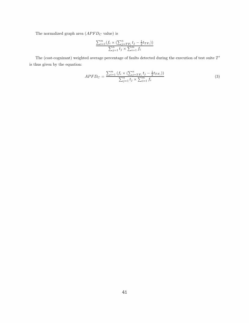
The normalized graph area (APFDC value) is

∑m

i=1(fi × (∑n

j=TFitj −

12 tTFi

))∑n

j=1 tj ×∑m

i=1 fi

The (cost-cognizant) weighted average percentage of faults detected during the execution of test suite T ′

is thus given by the equation:

APFDC =

∑m

i=1 (fi × (∑n

j=TFitj −

12 tTFi

))∑n

j=1 tj ×∑m

i=1 fi

(3)

41