Asymmetric Cost Behavior in Local Public Enterprises:

Exploring the Public Interest and Striving for Efficiency

This is a post-peer-review, pre-copyedit version of an article published in Journal of Management Control. The final authenticated version is available online at: http://dx.doi.org/10.1007/s00187-018-0269-x

Springer　発行Journal of Management Control　掲載

　2018年12月　Vol.29　No.3-4

1

Table of Contents

1 Introduction ........................................................................................................................................3

2 Background and Literature Review……………………………………………………………………7

2.1 Characteristics of LPEs……………………………………………………………………………7

2.2 Institutional Constraints of LPEs………………………………………………………………….9

2.3 Cost Behavior of Public Sector Organizations…………………………………………………...11

2.4 Hypothesis Development………………………………………………………………………....13

3 Research Method and Sample Selection…………………………………………………………..….16

3.1 Research Method…………………………………………………………………………………16

3.2 Sample Selection and Descriptive Statistics……………………………………………………..17

4 Results………………………………………………………………………………………………...18

5 Conclusions………………………………………………………………………………………...…23

References……………………………………………………………………………………………27

Appendix……………………………………………………………………………………………..31

2

Abstract

Asymmetric cost behavior, which was first identified in Germany in the 1920s, has attracted the

attention of researchers over the last two decades. Cost management is essential not only for commercial

enterprises (CEs) but also for public organizations. Therefore, in this research, I focus on local public

enterprises (LPEs), one type of public organization in Japan, and clarify their cost behavior. Then,

taking the perspective of institutional theory, I compare LPEs with CEs. Because LPEs are required to

behave according to the restrictions of LPE law, they are more vulnerable to institutional pressure.

Specifically, LPEs have two normative institutional constraints: (1) efficiency and (2) the public interest

(i.e., the responsibility to support people’s everyday lives). Therefore, LPEs must provide certain

services even if they are unprofitable. To explore whether normative institutional pressure causes LPEs

to be cost inefficient, I compare the cost behavior of these enterprises with that of CEs in five ways. I

analyze (1) panel data covering 40 years, (2) the change over time, (3) the differences by industry type,

(4) the relationship with population changes, and (5) the effect of political influence. I find that LPEs’

cost management is not necessarily cost inefficient; however, their ability to adjust costs may be lost in

the future due to the influence of institutional constraints. I therefore assert that LPE administrators

must constantly struggle to balance the institutional constraints of the public interest and efficiency

since these factors require long-term, stable management.

Keywords: local public enterprises, sticky costs, anti-sticky costs, asymmetric cost behavior, public

interest, efficiency, institutional constraints

JEL codes: H83, M41

3

1 Introduction

After World War II, public enterprises (PEs) were created in both developed and developing

countries to address market deficits and capital shortfalls, promote economic development, reduce mass

unemployment and/or ensure national control over the overall direction of the economy (UN, 2008).

Over the long term, PEs provided public services that were directly managed by governments. However,

management inefficiencies, overstaffing, inflation and rising current account deficits in the 1980s

exposed serious “government failures” and the limitations of PEs as major players in economic

development (UN, 2008). Subsequently, new public management (NPM) led public organizations

(including PEs) to change their behavior from reflecting administrative aspects to reflecting managerial

aspects (Van Genugten 2008; Pérez-López et al. 2015). From the perspective of fiscal finance, the

operations of public organizations switched from recognizing soft budget constraints to recognizing

hard budget constraints (Bertero and Rondi 2000). Furthermore, in the 1990s, many public services

provided by public sector organizations were outsourced or the organizations were privatized and

became commercial enterprises (CEs) because of pressure to improve their efficiency and effectiveness

(Hefetz and Warner 2007). Thus, public service costs in public sector organizations were initially

reduced through outsourcing or privatization (Domberger and Jensen 1997; Domberger and Rimmer

1994; Hodge 2000), but the cost reduction effects gradually decreased over the long term (Bel and

Costas 2006; Dijkgraaf and Gradus 2011). Therefore, in the 2000s, the responsibility for outsourced

public services shifted again to corporatized PEs, which emphasize efficiency and have greater

independence from the government than PEs that are directly managed by governments (Hefetz and

Warner 2007; Grossi and Reichard 2008; Wollmann et al. 2010). Currently, various public services are

provided by corporatized local public enterprises (LPEs) in every region of the world (Saussier and

Klien 2013) (Table 1).

[Insert] Table 1. LPEs in selected countries

Recently, corporatized LPEs1 have been found to be more efficient than LPEs directly managed by

local governments (Voorn et al. 2017). Nevertheless, LPEs are generally considered to be more cost

inefficient than CEs since the former face stronger institutional pressure (i.e., normative, coercive, and

mimetic) than CEs (Frumkin and Galaskiewicz 2004). In particular, from the viewpoint of normative

institutional constraints, LPE administrators are pressured by law to achieve efficiency2 and serve the

public interest3. However, it is very difficult for LPE administrators to do both simultaneously. If LPE

administrators prioritize cost reductions due to the influence of efficiency pressures, the risk of

1 Hereafter, in Section 1, “LPEs” refer to corporatized LPEs. 2 The concept of efficiency is used differently in each study focusing on the public sector (Voorn et al. 2017). In this article, efficiency refers to cost efficiency. 3 The concept of the public interest can be defined not only as a specific conceptualization of the term “public interest” but also with a variety of meanings from very specific to very broad definitions (Pesch 2005; Van Genugten 2008). Therefore, in this research, following De Bruijn et al. 2004, “public interest” is defined as both the importance of services (i.e., necessary and convenient for everyday lives) and the roles and responsibilities of governments.

4

declining public service quality increases. Conversely, pursuing the public interest can lead LPE

administrators to manage their costs more inefficiently. Thus, LPE administrators must strike a balance

between efficiency and the public interest under the pressure of these two normative institutional

constraints (Kawarata 2005). By contrast, CE managers aim only to maximize profits; since they are

subject to fewer institutional pressures than LPEs, they have greater flexibility in making management

changes (Eldenburg et al. 2004; Balakrishnan et al. 2010; Holzhacker et al. 2015). However, to date,

research on whether public services are more inefficiently performed by LPEs than CEs is lacking.

Therefore, my research question is whether LPEs manage their costs more inefficiently than CEs. In

this research, I focus on LPEs in Japan and clarify their cost management. In addition, I compare my

results with those for CEs based on the theoretical background of institutional theory. I choose Japanese

LPEs for two reasons. First, the number of LPEs in Japan is very high compared to the number

worldwide (Table 1). In Japan, the Local Public Enterprise Law was enacted in 1948, after World War II,

and subsequently, many LPEs were established in each municipality. Therefore, it is possible to collect

data from a large cross-sectional sample, making this empirical research more robust. Second, LPEs are

consistently the main bodies providing public services and have been continuously engaged in this

important role supporting civil life in Japan over the long term. Therefore, it is possible to collect

consistent, long-term time series data. The accounting system for LPEs remained unchanged until 20144.

Therefore, in this research, I was able to collect fiscal data from 19745 to 2013 and verify the long-term

changes in cost management alongside the global trends for each period, for example, the trends in

NPM since the 1980s, outsourcing or privatizing into CEs since the 1990s, and the revival of LPEs since

the 2000s.

Additionally, I discuss how LPEs’ cost management should be sustainably controlled in the future

not only in theory but also in practice. LPEs in Japan have encountered two main issues in recent years

that have intensified the institutional constraints of achieving efficiency and serving the public interest:

population changes and a deteriorating financial situation. According to Japan’s population census, the

country’s population had reached its upper limit and entered a stage of decline (Figure 1). In Japan, the

proportion of elderly people in the total population exceeded 14% in 1995, and Japan became an aging

society. Furthermore, in 2007, this proportion exceeded 21%, representing a super-aging society. In

conjunction with this shift, the population of youth and of those in the productive ages has continued to

decline. Additionally, Japan’s suburban population has decreased dramatically. The Japanese

government reported that the percentage depopulated areas6 of Japan has increased from 40.7% in 1972

4 LPEs in Japan adopted almost the same bookkeeping method as CEs beginning in 1966. After 2014, the accounting standards of LPEs have changed. Many of them are based mainly on changes in the balance sheet that this research does not pay attention to. On income statements (P/L) that I pay attention to in this study, the method of amortizing fixed assets when purchased with subsidies has been changed. Before 2013, the amortizing fixed assets were accounted for only in expenses; on the other hand, after 2014, the amortizing fixed assets were accounted for not only in expenses but also in revenue, as the long-term advances received. 5 1974 is the first year for which data collection was possible. 6 The depopulated areas in Japan are defined in the Act on Special Measures for Promotion for Independence for Underpopulated Areas. There are many requirements for specifying depopulated

5

to 58.7% in 2015. The number of depopulated municipalities also increased from 32.3% in 1972 to

46.4% in 2015. LPEs must continue their businesses despite the institutional constraint of serving the

public interest, even if the costs of idle capacity rise due to a declining number of users caused by

population decreases. Conversely, the aging population, who need more public services (e.g., medical

services, care services) at a low cost, will continue to increase in the future.

[Insert] Figure 1. Population changes in Japan

A final issue is the difficulty LPEs experience in repaying bonds (Figure 2 Panel A). LPEs issue

bonds to finance new public service projects (including both maintenance and renovation projects) or to

improve the quality or expand the quantity of public services. In examining LPEs’ financial statements,

although operating revenues and expenses may be in surplus, non-operating revenues and expenses

often show deficits (Figure 2 Panel B and Panel C). This difference is due mainly to the repayment of

bonds and interest payments. Since interest payments are a fixed cost, LPE administrators must reduce

other variable costs. However, cost adjustment flexibility decreases with increases in LPE bonds.

Namely, the repayment of LPE bonds requires LPE administrators to further enhance their organizations’

efficiency.

[Insert] Figure 2. LPE bonds, operating and non-operating revenues and expenses

For LPEs to improve their efficiency, it is essential to consider further developing their cost

management. Thus, clarifying LPEs’ cost behavior and understanding its movement is important for

improving LPEs’ cost management (Murray 1975; Rainey et al. 1976). In research on cost behavior,

German studies identified “Kostenremanenz” in the 1920s. Over the past 20 years, this phenomenon has

again attracted the attention of empirical researchers in management accounting (Noreen and

Soderstrom 1997) and is now known as “sticky costs (cost stickiness)” (Anderson et al. 2003). Sticky

costs increase proportionally as activities increase, but when activities decrease, the costs do not

decrease symmetrically. In subsequent studies, sticky costs were found to exist in each region, country

and industry (Calleja et al. 2006; He et al. 2010; Subramaniam and Weidenmier 2016). Conversely, it

has also been verified that a change in cost may exceed the change in activity (Weiss 2011). Subsequent

empirical research showed that cost behavior includes not only sticky costs but also anti-sticky, i.e.,

asymmetric, costs when activity increases and decreases (Banker and Byzalov 2014). However, most

previous studies have focused on CEs (Malik 2012; Günther et al. 2014), and only a few studies have

focused on public sector organizations’ cost behavior (Yasukata et al. 2011; Bradbury and Scott 2014;

Cohen et al. 2014; Holzhacker et al. 2015). Therefore, the goal of this research is to examine LPEs’ cost

behavior, which has not yet been analyzed. In addition, I examine whether LPEs’ cost behavior reflects

high or low sticky costs when compared to CEs from the viewpoint of institutional theory through a

areas: one is that the population declined more than 33%.

6

long-term empirical analysis.

Through this study, I contribute five findings to the cost behavior research. First, I find that LPEs’

cost management is not necessarily inefficient compared to CEs from the perspective of cost behavior.

Namely, I find that sticky costs exist in CEs’ cost behavior, and conversely, anti-sticky costs are

revealed in LPEs through a panel data analysis covering 40 years. In addition, I discovered that LPEs’

cost behavior contrasts with that of CEs. However, these results also contrast with the expected

conclusions in general. I believe that the lack of support for this expectation might be driven by

accounting system (regulations on dividends and retained earnings) and management system

(redundancies; e.g., preparation for disasters) differences between CEs and LPEs.

Second, I discovered that after a certain period of time has passed from LPEs’ establishment,

inefficient risks in LPEs’ cost management are caused by institutional pressure to protect the public

interest. Through a timeline (year by year) analysis over 40 years, I find that LPEs’ cost behavior

gradually shifted from anti-sticky costs to sticky costs. This result also contrasts with CEs’ cost behavior,

which did not drastically change. I discovered that the adjustment ability of management resources in

LPEs was gradually lost over the long term. From the viewpoint of securing the public interest, obsolete

equipment must be repaired or replaced to maintain the quality of public services, even if revenues

decrease. I conjecture that cost-inefficient risk is affected by an increase in the costs of facilities and

equipment.

Third, through an analysis by industry type, I find various characteristics of LPEs’ cost behavior in

each industry type, including high material resource industries and high human resource industries. The

diversity of cost behavior in LPEs might be caused by the resource adjustment costs in various business

environments and the various institutional restrictions, including the non-exclusion of public services

and the influence of monopolies.

Fourth, I discovered that depopulation and structural changes in the population influence LPEs’ cost

behavior. Since population change is closely related to public service demand, the administrators of

LPEs need to manage those costs that respond sensitively to population changes. I can show how public

service providers should adjust their costs due to population changes, which suggests that the influence

of population changes must be taken into consideration to preserve LPEs’ cost adjustment ability.

Finally, I clarify how LPE administrators adjusted their costs based on changing activity levels over

four years, which equals politicians’ term in office, and verify the differences between LPEs and CEs. I

find the cost behaviors’ differences in both the speed of change and the direction of movement can be

compared. Regarding the changing speed of cost behavior, LPE administrators try to adjust their costs

so that they remain proportional over four years, as they aim to operate their services in a stable manner

and attempt to balance the public interest and efficiency sustainably. Regarding the direction of

movement, one might assume that LPE administrators are subject to institutional pressure from

politicians, who respond to public opinion, and social demands, which require the enrichment of public

services rather than excessive cost efficiency. I conjecture that LPE administrators intend to adjust their

costs to balance their proportions during politicians’ term in office.

In addition, by understanding the characteristics of LPEs’ cost behaviors from an academic

perspective, it will be possible to contribute to public administrators’ ability to manage their future costs.

7

I also contribute to practical aspects of LPE cost management in the future sustainability plans called the

Compact City and Intermunicipal Cooperation.

The article proceeds as follows. Section 2 discusses the characteristics of LPEs from the viewpoint

of institutional theory, reviews the literature on public organization cost behavior and develops my

research hypotheses. In Section 3, the research methodology is described, including the sample data, the

variable measures, and the models. Section 4 presents and discusses the results. Finally, Section 5

summarizes the results and concludes with a discussion of the limitations of this study and suggestions

for future research.

2 Background and Literature Review

2.1 Characteristics of LPEs

Since World War II, LPEs have been an important public service provider not only in developed

countries throughout the world but also in developing countries (UN, 2008). LPEs are called various

names within each country and region, such as “municipally owned enterprises”, “municipal

corporations”, “local public companies”, “municipal corporatizations”, and “state-owned enterprises”

(Collin et al. 2009; Saussier and Klien 2013; Voorn et al.2017).

A UN (2008) report defined public enterprises as follows: a “public enterprise can be considered an

organization established by the government under public or private law, as a legal personality which is

autonomous or semi-autonomous, that produces/provides goods and services on a full or partial

self-financing basis, and in which the government or a public body/agency participates by way of

having shares or representation in its decision-making structure”. However, in the academic field, there is no definite and common definition of a public enterprise to

date (Collin et al. 2009; Saussier and Klien 2013) because LPE regulations differ from country to

country and LPEs’ service content differs from region to region. Thus, it can be stated that LPEs exist in

an institutional twilight area, as they are both public administrators and private companies (Collin et al.

2009). Because of the existence of various forms and types of LPEs in each country and region,

academics to date have not recognized common LPE issues. Based on a taxonomy, Saussier and Klien

(2013) classified LPEs based on decision-making rights, organizational control, and property rights.

They distinguished between directly managed LPEs and corporatized LPEs. Additionally, Voorn et al.

(2017) described the unique features of directly managed LPEs and those of corporatized LPEs (Table

2).

[Insert] Table 2. Characteristics of directly managed LPEs and corporatized LPEs

Saussier and Klien (2013) explained that Japanese LPEs are part of the local public government and

are not independent organizations. Therefore, they argued that Japanese LPEs are not suitable as

subjects of empirical research because they are not financially and organically separate from local

public governments. LPEs in Japan are certainly a type of public organization owned by local

governments. However, I assert that the researchers’ argumentation is partly correct and partly wrong.

According to their taxonomy, LPEs in Japan are classified into directly managed LPEs and corporatized

8

LPEs. The former are part of local public bodies, as these authors claim, but the latter are run

independently. The services provided by corporatized LPEs are funded by user fees, and the entities

must be profitable independently of local public bodies. Thus, corporatized LPEs have weaker

regulations than directly managed LPEs and can be managed flexibly using their income from utilities.

It is expected that the efficiency and effectiveness of the services provided by corporatized LPEs will be

promoted over services provided by directly managed LPEs (Oshima 1971). Therefore, I argue that

corporatized LPEs in Japan are suitable for empirical analysis because they are financially and

organically separate from local public governments.

In Japan, legislation established LPEs in each municipality after World War II. The number of LPEs

increased with the increase in population: there were 6,995 enterprises in 1974, 12,629 enterprises in

2002, when they reached a peak, and recently, after a decline due to privatization or amalgamation, there

were 8,712 enterprises in 2013 (Figure 3). In addition, there are more directly managed LPEs than

corporatized LPEs. However, the number of directly managed LPEs has decreased substantially since

2004 under the influence of privatization based on the institutional pressure of NPM. By contrast, the

number of corporatized LPEs has not changed drastically for 40 years. I argue that corporatized LPEs

are also appropriate for empirical analysis because the number of such organizations is larger than that

in other countries, and data collection is possible over a longer period. For this reason, I focus on

corporatized LPEs for this analysis.

[Insert] Figure 3. Trends in the number of LPEs in Japan

Corporatized LPEs (hereafter, LPEs) are governed by an administrator appointed by the mayor and

approved by congress for a four-year term in office. Dismissal is restricted during this term. The

administrator has decision rights regarding the management of an LPE. Therefore, the administrator is

similar to the CEO of a CE. However, unlike CEOs, LPE administrators are not allowed to receive

dividends from the organization’s profits. Therefore, from the perspective of agency costs, there is little

incentive for administrators to declare a high amount of dividends (Eldenburg and Krishnan 2003).

However, if the administrator achieves a high level of performance (e.g., high evaluation of the service,

cost reductions), the mayor can reappoint the administrator. Therefore, the administrators of LPEs may

strive to achieve high performance with regard to serving the public interest and achieving efficiency. In

other words, administrators may be indirectly influenced by politics (congress and the mayor).

Additionally, LPEs’ budget must be approved by both congress and the mayor, which means that LPE

administrators are accountable to both parties. Therefore, the administrators of LPEs may face

institutional pressure from stakeholders such as congress and the mayor.

LPEs are responsible for various public service businesses that complement the public services

offered by local governments (Ooshima 1971; Kawarata 2005). More specifically, LPEs in Japan are

businesses that act under the LPE law and municipal ordinances. Examples of businesses in which LPEs

operate include residential water supply, industrial water supply, transportation (e.g., tramway, bus, and

subway), electricity, gas power, hospitals, and other businesses that are run by local governments

according to their own rules (Table 1). These businesses not only require a large amount of investment

9

that cannot be procured by the private sector but also will not necessarily be profitable for CEs.

Therefore, LPEs provide essential, lifesaving activities that cannot be managed as CEs based on

economic principles. For these reasons, administrators must attempt to recover the invested funds

appropriately and make decisions that prevent losses (Yasukata et al. 2011). Additionally, they must be

accountable to congress and the mayor in terms of securing profits and improving benefits for the public

(Eldenburg and Krishnan 2008).

2.2 Institutional Constraints of LPEs

Institutions are social structures consisting of symbols, social actions and objectives, but institutions

are formed not only through social structures but also through the activities in which norms and rules

are produced. In its present form, the new institutionalism in organizational analysis provides a wide

range of theoretical and methodological benefits (Scott 2001). Neo-institutional theorists, e.g., Meyer

and Rowan (1977), noted that organizations engage in normative organizational behavior based on rules,

laws, customs, traditions, and regulations with an emphasis on legitimacy, satisfactory behavior,

structural decoupling, and symbols. They also explained that organizations pursue practices that may be

of little relevance to maximizing efficiency and that organizations constantly seek ways to respond to

pressure from external scrutiny and regulations rather than improving their performance. DiMaggio and

Powell (1983) identified three forces that drive institutionalization: (1) coercive isomorphism, which

stems from political influence and the need for legitimacy; (2) mimetic isomorphism, which results from

standard responses to uncertainty; and (3) normative isomorphism, which is associated with

professionalization. Among them, normative institutional pressure constrains both decision-making and

organizational behavior (Balakrishnan et al. 2010; Holzhacker et al. 2015).

Public organizations promote mainly normative institutionalization in for-profit and nonprofit

organizations since public organizations can establish rules, laws, and regulations and provide licenses

and inspections. However, public organizations experience strong institutional pressure with regard to

their role governing profit and non-profit organizations (Frumkin and Galaskiewicz 2004). Balakrishnan

et al. (2010) also argued that the influences of institutional constraints are stronger for public

organizations than for for-profit organizations. The authors showed that normative institutional

constraints include political pressure, legal compatibility, the corporate governance system, and

financial support. As evidence of normative institutional pressure that constrains both decision-making

and organizational behavior, Wollmann (2000) explained that local German governments have changed

their organizational structures based on the institutional pressure of NPM. One of the reasons for the

strong influence of institutional constraints is that public organizations must respond to

multidisciplinary evaluations at all times due to the existence of an unspecified number of stakeholders

(Rainey 1997). Therefore, these organizations act to acquire legitimacy by observing institutional norms

such as rules, laws, and regulations (Oliver 1991; Nee and Cao 2005), which makes them sensitive to

normative institutional pressure (Frumkin and Galaskiewicz 2004).

For LPEs, there are two behavioral standards (codes of conduct) mandated by LPE law to stabilize

public services and to continue the business over the long term: first, fulfilling public demands to satisfy

the public interest, and second, pursuing appropriate profits by focusing on profitability and optimizing

10

costs by improving efficiency. LPEs must adopt a strict code of behavior and conduct their business

while confronting these two normative pressures. In particular, from the perspective of the public

interest, LPEs offer public services that are essential to citizens’ lives. This system covers the provision

of public goods and services in a comprehensive manner that complements the public services provided

by local governments from the public interest perspective. In addition, the level of public service must

always be kept constant since declining quality can threaten livelihoods. Thus, LPEs have a

responsibility to support everyday lives and provide improved public benefits through their

organizational behavior. Additionally, the evaluation of public services is conducted by all citizens, that

is, an unspecified number of people. Because such evaluations are multifaceted, as Rainey (1997) noted,

the administrators of LPEs must be concerned about serving the public interest. Thus, LPEs must

provide public services even if they are unprofitable (Ooshima 1971; Kawarata 2005). As a result,

institutional pressures also affect the cost-management decisions made by the administrators of

government hospitals, which are a type of public organization (Balakrishnan et al. 2010). However,

because the public interest must be balanced with efficiency, administrators cannot prioritize one over

the other (Eldenburg et al. 2004). Conversely, with regard to efficiency, LPEs must provide services

more economically, effectively, and efficiently than local municipalities (Kawarata 2005), which means

that they must operate with limited assistance from the government. Moreover, raising public utility fees

is not easy because it will be opposed by residents. Therefore, LPE administrators must manage their

organizations to avoid service charge increases as much as possible. As a result, they may have anxiety

due to the need for cost management and efficiency.

Because of these normative institutional constraints, LPEs’ organizational behavior differs greatly

from that of CEs. CEs act to maximize profits; because they are subject to fewer institutional pressures,

they have greater flexibility when making changes (Eldenburg et al. 2004; Balakrishnan et al. 2010;

Holzhacker et al. 2015). Therefore, institutional constraints more strongly affect the cost behavior of

public organizations than that of for-profit organizations (Holzhacker et al. 2015). To confirm the

characteristics of public organizations, research methods that compare these organizations with a control

group, either for-profit or nonprofit organizations, are generally adopted (Sørensen 2007; Balakrishnan

et al. 2010; Holzhacker et al. 2015). Therefore, I verify LPEs’ cost behavior by comparing these

organizations to CEs from the perspective of institutional constraints. Table 3 summarizes the

differences in the institutional pressure experienced by LPEs and CEs according to Eldeburg et al.

(2004) and Balakrishnan et al. (2010).

[Insert] Table 3. Organizational type and expected influence on cost behavior

In their governance systems, LPEs have fewer executives than CEs. Thus, LPEs usually have only

one administrator and a few vice administrators. For this reason, the pressure from stakeholders is

concentrated on the administrators; therefore, the administrators may focus on maintaining public

service standards at a low cost in order to gain legitimacy. In terms of legal compliance, unlike CEs,

which aim only to maximize profits, LPEs are required to pursue both the public interest and efficiency.

Furthermore, in terms of political pressure, LPE administrators are accountable to residents, the local

11

parliament and the mayor with regard to public service quality and cost management. If LPE

administrators prioritize cost reductions due to the influence of efficiency pressures, the risk of

declining public service quality will increase. Conversely, pursuing the public interest can lead LPE

administrators to manage their costs more inefficiently. Thus, LPE administrators must govern their

organizations while considering both the public interest and efficiency, and they must behave in a

manner that ensures business continuity (Kawarata 2005; Martinsons et al. 2007).

2.3 Cost Behavior of Public Sector Organizations

The concept of cost stickiness originated in the latter half of the 1920s. In Germany, Brasch (1927)

termed this phenomenon “Kostenremanenz”, and this notion was clarified through the direct observation

of companies’ cost information. Recently, “Kostenremanenz” has attracted the attention of empirical

analysts; the German term has since been translated to “cost stickiness” (“sticky costs”) by Anderson et

al. (2003). Those authors examined 7,629 firms over 20 years, from 1979 to 1998, using annual

Compustat data. In addition, they verified firms’ cost behavior using models based on published

financial data to determine the rate of change in net sales revenue (a proxy for the activity level as an

explanatory variable) and the rate of change for selling, general and administrative expenses (a proxy

for cost variables and the dependent variable). They found that the rate of change for costs when the

activity level decreases is smaller than it is when the activity level increases (Figure 4).

[Insert] Figure 4. Image of sticky costs and anti-sticky costs

Figure 4 shows that cost and revenue change proportionately and linearly with respect to the normal

t-1 phase of the slope from the t-1 to the t period, but sticky costs result in a slope that is less steep than

the slope near the t-1 period. Thus, “Kostenremanenz” is empirically confirmed as “cost stickiness”.

With regard to additional evidence of cost stickiness, since Anderson et al. (2003), sticky costs have

been verified through additional empirical research using those authors’ model and have also been

confirmed to exist in other scenarios, such as inter-industry and inter-country scenarios.

In a study focused on inter-industry scenarios, Subramaniam and Weidenmier (2016) examined cost

behavior by industry using Compustat data from 1979 to 2000. They showed that cost stickiness is

stronger in the manufacturing industry, which has more fixed assets, than in the merchandising, service

and finance industries. However, He et al. (2010) examined the cost behavior of Japanese CEs by

industry type from 1975 to 2000 using the PACAP database. They showed that the merchandising

industry has stickier costs than the service and manufacturing industries. As described above, various

cost behaviors have been confirmed for each industry for CEs. In addition, sticky costs were confirmed

not only in industries with high material resources but also in industries with high human resources.

In studies focused on inter-country scenarios, Calleja et al. (2006) performed an analysis using

financial data for US, UK, German, and French firms from 1988 to 2004. Their findings confirmed that

German and French firms demonstrate stronger sticky costs than firms in the UK and US. The authors

noted the possibility that differences in corporate governance and managerial oversight driven by the

regulation laws in each country and the characteristics of each firm and each type of industry may also

12

affect sticky costs. Using Compustat data from 1988 to 2008, Banker et al. (2013) showed that the

different worker protection regulations in 19 OECD countries affected labor adjustment costs. These

studies suggested that as industries become more regulated by law, their cost adjustment flexibility

decreases. LPEs that are highly subject to legal institutional restrictions may have a lower degree of

freedom regarding cost management than CEs. In previous studies targeting CEs, the analysis period has

mainly been set at approximately 20 years or less. Since public service providers are required to have

stable management over the long term (longer than 20 years), it is necessary to further understand their

long-term cost behavior.

Researchers have classified cost behavior for not only sticky costs but also anti-sticky costs (Weiss

2011). Figure 4 shows that anti-sticky costs also result in a slope that is initially steeper but that grows

less steep as it approaches the t period. Thus, anti-stickiness results when the slope of costs for

increasing activities is lower than the slope of costs for decreasing activities. Dalla Via and Perego

(2014) confirmed the existence of anti-cost stickiness for small and medium-sized enterprises. At the

same time, they noted that cost stickiness increases in large firms. Likewise, Sepasi and Hassani (2015),

and Boshch and Blandon (2011) also showed that cost stickiness is higher in large enterprises when

comparing large enterprises to small and medium-sized enterprises. These studies show that sticky costs

increase when the adjustment costs (committed capacity costs) for capacity resources such as

high-intensity assets or labor in large companies are high. That is, when the resource adjustment cost is

high, it is difficult to adjust costs according to changes in the activity level (Banker et al. 2014a).

Conversely, since the capacity resources of small and medium enterprises consists mainly of variable

costs, anti-sticky costs emerge. Günther et al. (2014) organized and described the relationship between

holding costs and adjustment costs based on the prior cost stickiness literature. The authors explained

that the factors influencing cost stickiness can be classified into three relationship types: (1) high

adjustment costs attributable to legal requirements or economic and psychological issues; (2) high

holding costs attributable to opportunity costs; and (3) high holding costs attributable to social issues.

To date, most studies have focused only on CEs, and only a few empirical studies of cost behavior

have focused on public organizations. Bradbury and Scott (2014) conducted an empirical analysis of the

cost behavior of New Zealand’s public municipalities from 2008 to 2012. In New Zealand,

cost-management methods similar to those used by CEs have been introduced into public organizations

since the 1980s as part of an NPM plan to improve the effectiveness and efficiency of administrative

activities. With thirty years having passed since 1980, these authors examined whether cost management

improved after 2008. However, the research showed that sticky costs continued to exist in New

Zealand’s local governments and that the efficiency of local government activities had not yet improved.

Cohen et al. (2017) investigated the cost behavior of Greek local governments, which was a cause of the

Greek fiscal crisis. These authors verified asymmetric cost behavior for different cost categories.

Specifically, they focused on the difference between administrative costs and the costs of service

provision by empirically describing the cost behavior. They found that the costs of service provision (a

core competence of local governments) were sticky, and administrative costs were anti-sticky. These

authors asserted that this asymmetric cost behavior was influenced by the decisions of local government

administrators, who were pressured by politicians and stakeholders. Additionally, they argued that local

13

government administrators cannot decrease the cost of service provision in response to external

pressures, even if revenues have decreased because of a fiscal crisis. Holzhacker et al. (2015) focused

on the differences between the institutional pressures on government hospitals and those on for-profit

and nonprofit hospitals and found differences in cost behaviors. Specifically, sticky costs were prevalent

in government hospitals, which were subject to strong institutional pressures. The authors argued that

one reason for their research results is that government hospitals need to take normative actions because

of stakeholders’ excessive pressure. The taxes, subsidies or donations from stakeholders such as local

communities or citizens’ groups force government hospitals to behave for the public interest. Yasukata

et al. (2011) showed the existence of sticky costs in the Japanese National Hospital Organization,

suggesting that sticky costs appeared within labor costs because the Japanese National Hospital

Organization was strongly influenced by institutional pressures to not dismiss employees.

In analyses of these public organizations, there has been no focus to date on LPEs. LPEs have

unique characteristics among public organizations because they are required to act not only in the public

interest (similar to public organizations) but also in the interest of efficiency (similar to CEs). Therefore,

it is academically interesting to investigate how LPEs’ cost behavior has changed because such changes

reflect the pressure to act in the interest of both the public and efficiency (Figure 5).

[Insert] Figure 5. The causal relationship between the institutional constraints on and the cost behavior

of LPEs

2.4 Hypothesis Development

Based on the model developed by Anderson et al. (2003), asymmetric cost behavior, especially

sticky costs, has been evaluated in empirical studies focused on CEs. Using the same method, the

asymmetric cost behavior of local governments was confirmed by Bradbury and Scott (2014) and Cohen

et al. (2017). Holzhacker et al. (2015) found that the degree of sticky costs was greater in public

hospitals than in private hospitals because for-profit organizations have fewer institutional restrictions

than do public organizations. Therefore, the latter can change their governance or cost structure to

respond flexibly to increase their efficiency (Eldenburg et al. 2004; Eldenburg and Krishnan 2008;

Balakrishnan et al. 2010; Holzhacker et al. 2015). Further, public organizations are more strongly

influenced by institutional pressure than CEs (Frumkin and Galaskiewicz 2004). Therefore, it is

theorized that sticky costs can be confirmed in LPEs, given that these organizations have characteristics

similar to both public and private organizations. Additionally, LPEs are subject to the institutional

restrictions that service levels must be maintained without generating profits. Therefore, sticky costs

will be more prevalent in LPEs than in CEs. Thus, the first hypothesis is as follows:

Hypothesis H1: Sticky costs are more prevalent in local public enterprises than in commercial

enterprises.

Günther et al. (2014) argued that asymmetric cost behavior is affected by adjustment costs, such as

legal requirements. LPEs are legally required by LPE law both to work in the public interest and to

14

maximize efficiency. In addition, LPE administrators are influenced by various stakeholders against the

background of the two normative institutional constraints. Therefore, they are required to maintain the

public service level at a low, stable cost. In other words, pressures to prioritize efficiency will weaken

the sticky costs of LPEs from the cost behavior perspective. Conversely, pressures to prioritize the

public interest will boost LPEs’ sticky costs because public service quality must be maintained, even if

revenues decrease. To maintain their service level, LPEs must renew or replace aging facilities over the

long term, and they must plan for these costs without increasing their service charges. When LPE

administrators are subject to strong institutional constraints, they cannot make decisions quickly

(Martinsons et al. 2007) and will put off these problems to the future. Sometimes, facilities can be

repaired early in the business cycle, but after many years, it is often better to replace these facilities than

to repair them. In these cases, the replacement or repair costs may drastically increase, and LPEs’

resource adjustment ability will gradually be lost. Thus, it is believed that their cost behavior will

change based on the influence of institutional constraints, especially the requirement to protect the

public interest. Therefore, LPEs may take more time to balance their obligations due to the institutional

constraints of both protecting the public interest and achieving efficiency. Thus, the next hypothesis is as

follows:

Hypothesis H2: Institutional pressures are associated with the change in local public enterprises’

cost behavior over time, in contrast to that of commercial enterprises.

Subramaniam and Weidenmier (2016) revealed that sticky costs are stronger in manufacturing

industries with more fixed assets than in the commercial, service and finance industries. By contrast, He

et al. (2010) showed that the commercial industry’s sticky costs are higher than those of the service and

manufacturing industries. As described above, various asymmetric cost behaviors have been confirmed

for each type of industry for CEs, including cases with both high material resources (high fixed assets)

and high human resources (high labor costs). Anderson et al. (2003) argued that sticky costs will

increase when asset intensity and labor costs are high. LPEs’ businesses include not only high asset-type

industries, such as water supply and sewerage, but also high labor cost-type industries, such as

transportation and hospitals. Moreover, due to institutional constraints, various asymmetric cost

behaviors should appear in all businesses, as LPEs must balance serving the public interest and

achieving efficiency rather than only aiming to maximize profits, which is the goal of CEs. I conjecture

that sticky costs in LPEs will increase when these firms are pressured from the institutional constraint of

serving the public interest; conversely, LPEs’ sticky costs will decrease when they are pressured from

the institutional constraint of achieving efficiency. Thus, the next hypothesis is as follows:

Hypothesis H3: Similar to that of commercial enterprises, local public enterprises’ cost behavior is

associated with the type of industry.

Banker et al. (2014b) found that sticky costs increase when demand uncertainty or the downside risk

of demand increases. The demand for public services depends on population changes (Nakai 1988;

15

Nakano 2016). For this reason, the administrators of LPEs are required to predict changes in public

service demand based on population changes (Nishioka et al. 2007). In Japan, the population structure

has changed significantly since 1995. The population of youth and those of production age is

decreasing; conversely, the elderly population is increasing. Furthermore, the economy and demand are

experiencing a depression, and CEs are withdrawing from depopulated regions due to a lack of

profitability. Even if public demand decreases due to the declining population, LPEs cannot stop

providing services because of the institutional pressure to serve the public interest. In other words, from

the perspective of the public interest, LPEs cannot reduce the quality of their public services. In addition,

with the increase in elderly people, whose income is derived primarily from pensions, LPEs must

maintain the same level of public services at low prices because of the institutional pressure to achieve

efficiency. LPEs may experience increased sticky costs due to the downside risk of public demand and

public demand uncertainty. By contrast, the market demand for CEs is affected not only by domestic

trading but also by overseas trading, so they are less affected by population changes than LPEs. I

theorize that LPEs’ cost behavior will be more strongly influenced by population changes than that of

CEs. Thus, the next hypothesis is as follows:

Hypothesis H4: Local public enterprises’ sticky costs are strongly influenced by population changes

since 1995 in relation to commercial enterprises.

As noted by Bradbury and Scott (2014) and Cohen et al. (2017), local government administrators are

influenced by public opinion (demand for both low-cost and high-quality services) when they make cost

management decisions. Public organizations, including LPEs, must respond to multidisciplinary

evaluations at all times due to the existence of an unspecified number of stakeholders (Rainey 1997). In

particular, LPE administrators are appointed by the mayor and approved by congress, who are, in turn,

elected by citizens. Therefore, the administrators may be sensitive to not only public opinion but also

political opinion (from mayors and local councils) if they wish to be reappointed for the next term, and

they may strive to achieve a high level of performance with regard to protecting the public interest and

achieving efficiency. As a result, LPE administrators may act to control and adjust their asymmetric cost

behavior in the direction of symmetric cost behavior during the political term of mayors and local

councils, which is 4 years in Japan. Thus, LPE administrators must aim for a long-term balance between

protecting the public interest and achieving efficiency due to political pressure. Conversely, CEs’

business managers may decide to control and adjust their costs with a focus on securing profits as

quickly as possible, and they may not be as strongly affected by political pressure as LPEs. Thus

because of institutional constraints, LPEs’ long-term cost adjustments may be more controlled and move

more slowly than those of CEs. As a result, it is hypothesized that the administrators of LPEs make

decisions that result in asymmetric cost behavior that gradually transforms into a proportional

relationship over the long term. The final hypothesis is as follows:

Hypothesis H5: Local public enterprise administrators make decisions that result in the long-term,

proportional stabilization of cost behavior within a 4-year election period in

16

relation to commercial enterprises.

LPEs are characterized by serving the public interest and achieving efficiency. Thus, LPEs’ cost

behavior is presumed to change in the context of the tradeoff between the public interest and efficiency.

Because of the need to run businesses in a stable manner, LPE administrators make deliberate decisions

from a different perspective than that of CE managers.

3 Research Method and Sample Selection

3.1 Research Method

The analytical model of Anderson et al. (2003) is the basis of recent empirical studies of cost

behavior; it was adopted in studies following Anderson et al. (2003) and recently used by Bradbury and

Scott (2014), Cohen et al. (2017), and Holzhacker et al. (2015) to analyze the cost behavior of public

organizations. Therefore, this study assumes that the model can also be applied to the analysis of LPEs’

cost behavior. Thus, to verify hypotheses 1 to 3, I adopt model 1. To examine hypothesis 1, all the

samples are analyzed through panel data analysis using model 1. Next, to verify hypothesis 2, the

year-to-year changes in cost behavior are analyzed through OLS analysis using model 1. OLS analysis

was adopted to clarify the cost behavior in prior studies (Anderson and Lanen 2007; Zanella et al. 2015).

Thus, I intend to use not only panel data analysis but also OLS analysis to verify the existence of sticky

costs. Finally, for hypothesis 3, the samples for each type of industry are analyzed through panel data

analysis using model 1.

model 1

ln�𝐶𝐶𝐶𝐶𝐶𝐶𝐶𝐶𝑖𝑖,𝑡𝑡𝐶𝐶𝐶𝐶𝐶𝐶𝐶𝐶𝑖𝑖,𝑡𝑡−1

� = 𝛽𝛽0 + 𝛽𝛽1 ∗ ln�𝑅𝑅𝑅𝑅𝑅𝑅𝑅𝑅𝑅𝑅𝑅𝑅𝑅𝑅𝑖𝑖,𝑡𝑡𝑅𝑅𝑅𝑅𝑅𝑅𝑅𝑅𝑅𝑅𝑅𝑅𝑅𝑅𝑖𝑖,𝑡𝑡−1

� + 𝛽𝛽2 ∗ 𝐷𝐷𝑅𝑅𝐷𝐷𝐷𝐷𝑅𝑅𝐷𝐷𝐶𝐶𝑅𝑅_𝐷𝐷𝑅𝑅𝐷𝐷𝐷𝐷𝐷𝐷𝑖𝑖,𝑡𝑡 ∗ ln�𝑅𝑅𝑅𝑅𝑅𝑅𝑅𝑅𝑅𝑅𝑅𝑅𝑅𝑅𝑖𝑖,𝑡𝑡𝑅𝑅𝑅𝑅𝑅𝑅𝑅𝑅𝑅𝑅𝑅𝑅𝑅𝑅𝑖𝑖,𝑡𝑡−1

� + 𝜀𝜀𝑖𝑖,𝑡𝑡

LPEs’ operating expenses are substituted for Cost. Additionally, Revenue takes operating revenues

as a proxy for the activity amount. Decrease Dummy is a dummy variable that takes the value of 1 when

operating revenue decreases between the t period and the previous period and 0 otherwise. All the data

are natural logarithms.

Using this model, it can be confirmed that when operating revenue increases by 1%, the cost

changes by the value indicated by β1. Additionally, because of the Decrease Dummy, when operating

revenue decreases by 1%, the cost decreases by β1 + β2, whereas β2 indicates the value of the sticky or

anti-sticky costs. Therefore, when there is cost stickiness, β2 will be negative, and when cost stickiness

is not present (anti-sticky costs), β2 will be positive.

To examine hypothesis 4, I clarify the influence of the total population change and the population

structure on cost behavior. Therefore, I focus on population data from a report on population movement

based on a basic resident registration system database7. In particular, it is necessary to clarify the

7 Population data in each municipality is published as “Basic Resident Register Annual Population Report” by statistics bureau, ministry of internal affairs and communications in Japan.

17

influence of depopulation and the increasing ratio of the aging population on the cost behavior of LPEs.

For this reason, I collect population data from 1995, which is the year Japan started to become an aging

society. The population data were divided into three stages: 0-14 years old, 15-64 years old, and 65

years old and over. To evaluate hypothesis 4, I adopt the following model 2.

model 2

ln�𝐶𝐶𝐶𝐶𝐶𝐶𝐶𝐶𝑖𝑖,𝑡𝑡𝐶𝐶𝐶𝐶𝐶𝐶𝐶𝐶𝑖𝑖,𝑡𝑡−1

� = 𝛽𝛽0 + 𝛽𝛽1 ∗ ln�𝑅𝑅𝑅𝑅𝑅𝑅𝑅𝑅𝑅𝑅𝑅𝑅𝑅𝑅𝑖𝑖,𝑡𝑡𝑅𝑅𝑅𝑅𝑅𝑅𝑅𝑅𝑅𝑅𝑅𝑅𝑅𝑅𝑖𝑖,𝑡𝑡−1

� + 𝛽𝛽2 ∗ 𝐷𝐷𝑅𝑅𝐷𝐷𝐷𝐷𝑅𝑅𝐷𝐷𝐶𝐶𝑅𝑅_𝐷𝐷𝑅𝑅𝐷𝐷𝐷𝐷𝐷𝐷𝑖𝑖 ,𝑡𝑡 ∗ ln�𝑅𝑅𝑅𝑅𝑅𝑅𝑅𝑅𝑅𝑅𝑅𝑅𝑅𝑅𝑖𝑖,𝑡𝑡𝑅𝑅𝑅𝑅𝑅𝑅𝑅𝑅𝑅𝑅𝑅𝑅𝑅𝑅𝑖𝑖,𝑡𝑡−1

�

+ �𝛽𝛽𝑛𝑛

6

𝑛𝑛=3

𝑃𝑃𝐶𝐶𝑃𝑃𝑖𝑖,𝑡𝑡,𝑛𝑛 ∗ 𝐷𝐷𝑅𝑅𝐷𝐷𝐷𝐷𝑅𝑅𝐷𝐷𝐶𝐶𝑅𝑅_𝐷𝐷𝑅𝑅𝐷𝐷𝐷𝐷𝐷𝐷𝑖𝑖,𝑡𝑡 ∗ ln�𝑅𝑅𝑅𝑅𝑅𝑅𝑅𝑅𝑅𝑅𝑅𝑅𝑅𝑅𝑖𝑖,𝑡𝑡𝑅𝑅𝑅𝑅𝑅𝑅𝑅𝑅𝑅𝑅𝑅𝑅𝑅𝑅𝑖𝑖,𝑡𝑡−1

� + 𝜀𝜀𝑖𝑖,𝑡𝑡

The total population represents the natural logarithms of the year-over-year comparison. The young

population, the productive age population, and the elderly population are natural logarithms of each

respective proportion of the total population.

Next, to examine hypothesis 5, it is necessary to confirm the relationship between operating

revenues over 4 years and changes in operating expenses. I extend the model of Anderson et al. (2003)

and verify the hypothesis using the following model 3.

model 3

ln�𝐶𝐶𝐶𝐶𝐶𝐶𝐶𝐶𝑖𝑖,𝑡𝑡𝐶𝐶𝐶𝐶𝐶𝐶𝐶𝐶𝑖𝑖,𝑡𝑡−1

� = 𝛽𝛽0 + 𝛽𝛽1 ∗ ln�𝑅𝑅𝑅𝑅𝑅𝑅𝑅𝑅𝑅𝑅𝑅𝑅𝑅𝑅𝑖𝑖,𝑡𝑡𝑅𝑅𝑅𝑅𝑅𝑅𝑅𝑅𝑅𝑅𝑅𝑅𝑅𝑅𝑖𝑖,𝑡𝑡−1

� + 𝛽𝛽2 ∗ 𝐷𝐷𝑅𝑅𝐷𝐷𝐷𝐷𝑅𝑅𝐷𝐷𝐶𝐶𝑅𝑅_𝐷𝐷𝑅𝑅𝐷𝐷𝐷𝐷𝐷𝐷𝑖𝑖 ,𝑡𝑡 ∗ ln�𝑅𝑅𝑅𝑅𝑅𝑅𝑅𝑅𝑅𝑅𝑅𝑅𝑅𝑅𝑖𝑖,𝑡𝑡𝑅𝑅𝑅𝑅𝑅𝑅𝑅𝑅𝑅𝑅𝑅𝑅𝑅𝑅𝑖𝑖,𝑡𝑡−1

�

+𝛽𝛽3 ∗ ln�𝑅𝑅𝑅𝑅𝑅𝑅𝑅𝑅𝑅𝑅𝑅𝑅𝑅𝑅𝑖𝑖,𝑡𝑡−1𝑅𝑅𝑅𝑅𝑅𝑅𝑅𝑅𝑅𝑅𝑅𝑅𝑅𝑅𝑖𝑖,𝑡𝑡−2

� + 𝛽𝛽4 ∗ 𝐷𝐷𝑅𝑅𝐷𝐷𝐷𝐷𝑅𝑅𝐷𝐷𝐶𝐶𝑅𝑅_𝐷𝐷𝑅𝑅𝐷𝐷𝐷𝐷𝐷𝐷𝑖𝑖,𝑡𝑡−1 ∗ ln�𝑅𝑅𝑅𝑅𝑅𝑅𝑅𝑅𝑅𝑅𝑅𝑅𝑅𝑅𝑖𝑖,𝑡𝑡−1𝑅𝑅𝑅𝑅𝑅𝑅𝑅𝑅𝑅𝑅𝑅𝑅𝑅𝑅𝑖𝑖,𝑡𝑡−2

�

+𝛽𝛽5 ∗ ln�𝑅𝑅𝑅𝑅𝑅𝑅𝑅𝑅𝑅𝑅𝑅𝑅𝑅𝑅𝑖𝑖,𝑡𝑡−2𝑅𝑅𝑅𝑅𝑅𝑅𝑅𝑅𝑅𝑅𝑅𝑅𝑅𝑅𝑖𝑖,𝑡𝑡−3

� + 𝛽𝛽6 ∗ 𝐷𝐷𝑅𝑅𝐷𝐷𝐷𝐷𝑅𝑅𝐷𝐷𝐶𝐶𝑅𝑅_𝐷𝐷𝑅𝑅𝐷𝐷𝐷𝐷𝐷𝐷𝑖𝑖 ,𝑡𝑡−2 ∗ ln�𝑅𝑅𝑅𝑅𝑅𝑅𝑅𝑅𝑅𝑅𝑅𝑅𝑅𝑅𝑖𝑖,𝑡𝑡−2𝑅𝑅𝑅𝑅𝑅𝑅𝑅𝑅𝑅𝑅𝑅𝑅𝑅𝑅𝑖𝑖,𝑡𝑡−3

�

+𝛽𝛽7 ∗ ln �𝑅𝑅𝑅𝑅𝑅𝑅𝑅𝑅𝑅𝑅𝑅𝑅𝑅𝑅𝑖𝑖,𝑡𝑡−3𝑅𝑅𝑅𝑅𝑅𝑅𝑅𝑅𝑅𝑅𝑅𝑅𝑅𝑅𝑖𝑖,𝑡𝑡−4

� + 𝛽𝛽8 ∗ 𝐷𝐷𝑅𝑅𝐷𝐷𝐷𝐷𝑅𝑅𝐷𝐷𝐶𝐶𝑅𝑅_𝐷𝐷𝑅𝑅𝐷𝐷𝐷𝐷𝐷𝐷𝑖𝑖,𝑡𝑡−3 ∗ ln�𝑅𝑅𝑅𝑅𝑅𝑅𝑅𝑅𝑅𝑅𝑅𝑅𝑅𝑅𝑖𝑖,𝑡𝑡−3𝑅𝑅𝑅𝑅𝑅𝑅𝑅𝑅𝑅𝑅𝑅𝑅𝑅𝑅𝑖𝑖,𝑡𝑡−4

� + 𝜀𝜀𝑖𝑖,𝑡𝑡

If asymmetric cost behavior terminates over time, the sticky costs value will gradually approach 0. If

cost stickiness is confirmed by β2, it should change, β2 < β4 < β6, with time, since LPE administrators

are subject to institutional restrictions and will only gradually overcome the sticky costs. In particular,

political pressure is strengthened by politicians’ 4-year term. Additionally, local elections for congress

and the mayor of each municipality in Japan are held almost simultaneously on the same day. Therefore,

LPEs’ cost behavior may be influenced by political pressure. The analysis begins at t=0, which is an

election year, and elections are held in t=0, 4, 8, 12, etc.

3.2 Sample Selection and Descriptive Statistics

No empirical analysis of LPEs’ cost behavior has been previously performed. This research is

18

therefore the first to examine LPEs’ cost behavior. To obtain robust results, as much cross-sectional data

as possible should be used. I collected non-consolidated fiscal accounting data on all LPE businesses

from LPEs’ yearbooks8. Thus, the sample population for this analysis is all local public enterprise

businesses that are classified as corporatized LPEs. The data include 10 industry types (residential water

supply, industrial water supply, sewage, transportation, electric power, gas power, hospitals, wholesale

market, toll road, and car parking). In addition, observations must be made over a long period to

confirm how cost behavior has changed in accordance with changes in Japan’s social environment.

To verify LPEs’ cost behavior, long-term cost data are necessary. Therefore, in this study, the

analysis period is the 40 years from 1974 to 2013, which is a longer period than that analyzed by any

previous empirical studies on cost stickiness. LPEs are legally obligated to release annual financial

reports. The financial reporting method has not changed over the 40 years under study, making it

possible to collect fiscal data over a very long period. The collected data represent 120,317 firm-years.

To control for the effect of outliers, I removed (deleted) the largest and smallest 1 percent of

observations (outliers). I used list-wise case deletion without winsorized data to delete the observations.

That is, if there is even a single outlier in one sample, all the data from that sample are deleted (cleared).

This approach is rather conservative as a statistical method, but since there are numerous samples, I

contend that this approach is a valid statistical processing method to obtain robust analysis results. The

final sample includes 115,929 firm-years. Therefore, the sample consists of unbalanced panel data.

Additionally, to create a comparison with LPEs over the same period, I collected data provided by

Nikkei NEED-FinancialQUEST on CEs listed on the Tokyo Stock Exchange. LPEs’ financial statements

provide non-consolidated accounting data for various industry types, such as water supply and hospitals,

so I also collected CE non-consolidated accounting data from the Annual Securities Reports for

comparison. The collected data represent 85,705 firm-years. After excluding (deleting) outliers, the

sample includes 84,343 firm-years. The descriptive statistics are calculated after the exclusion of

outliers.

[Insert] Table 4. Descriptive statistics

4 Results

In panel data analysis, there is a process for choosing the optimal result from the model of pooled

estimates, fixed effects, and random effects. I describe all the analysis results and explain the optimal

results. First, in all panel data analyses, I used an F-test to determine whether a pooled model and a

fixed/random effects model is more suitable. The result confirms that the fixed/random effects model is

more suitable than the pooled model. In addition, I also conducted the Hausman test to confirm which

model, the fixed effects or random effects model, is suitable. In addition, I confirmed the influence of

8 LPEs’ yearbooks are edited annually by the ministry of internal affairs and communications in Japan. They include the annual financial statement of each LPE in each municipality. The financial statements include B/S, P/L, the detail information of expenses, etc.; these data are found in electronic databases after 1999.

19

serial correlation through the Durbin-Watson ratio. The influence of serial correlation is low in all the

analyses.

To test hypothesis 1 using model 1, I analyzed panel data for 40 years. The results showed that LPEs’

cost actions demonstrate asymmetric cost behavior (Table 5 Panel A). Namely, β2 was 0.0791 (fixed

effects), and the positive value indicates anti-sticky costs. Conversely, the CE analysis resulted in a β2

value of -0.0978 (fixed effects), and the negative value indicates sticky costs (Table 5 Panel B). Thus,

hypothesis 1 was not supported.

[Insert] Table 5. Cost behavior based on the panel data analysis using model 1

Under institutional constraints, it was predicted that sticky costs would increase because LPEs are

subject to stronger institutional pressures than CEs. However, the analysis resulted in the opposite

conclusion, which was not expected. In previous studies, no research showed that public organizations’

cost behavior was anti-sticky (Yasukata et al. 2011; Bradbury and Scott 2014; Cohen et al. 2017;

Holzhacker et al. 2015). Additionally, Banker and Byzalov (2014) argued that CEs’ cost behavior

generally indicated sticky costs on average. Clearly, this result is a new discovery that contrasts with

previous studies.

This result signifies that LPE administrators actively manage their resource-adjustable costs when

their operating revenue decreases and the pressure for low-cost economic efficiency increases. I believe

that the lack of support for this hypothesis might be driven by the accounting (regulations on dividends

and retained earnings) and management system (redundancies, i.e., preparation for disasters such as a

standby isolated power unit and food stockpiled for emergencies) differences between CEs and LPEs.

Namely, the anti-sticky costs are induced by resource-adjustable costs, which imply that there are

redundant resources caused by LPEs’ accounting and management systems.

Regarding the accounting system, I focus on the appropriation of retained earnings and the net

income of LPEs. The retained earnings of CEs are often allocated to stakeholders, such as shareholders,

managers, or workers. Unlike CEs, LPEs are subject to legal restrictions regarding how they can

appropriate retained earnings. Namely, it is unnecessary for LPEs to distribute their final profits to

stakeholders, such as shareholders, managers, and workers. Additionally, because they can receive

preferential treatment regarding corporate tax and property tax, their retained earnings may often be

generated. However, LPEs are required to operate with moderate profits and not to maximize their net

income. Therefore, I conjecture that LPE administrators intend to ensure their management resource

slack so that they can adjust quickly when operating revenue declines. Because the slack resources in

LPEs are oriented toward preventing disasters, they are not necessary for normal operations. Therefore,

there is a great deal of room for discretion; thus, it is easy to reduce these resources. In other words,

LPE administrators may increase their management resources, thus increasing their operating expenses,

in order to avoid significantly increasing their operating profits. In fact, as shown in Panel B of Figure 2,

operating expenses and operating revenues show very similar, consistent movements over the long term.

LPEs thus may accumulate excessive management resources rather than repaying their bonds. Because

LPEs have little risk of bankruptcy, they may not make the effort to repay their debt; on the contrary, it

20

is possible that they intend to bear the cost of procuring excessive management resources accordingly.

Therefore, they can use their profit for management resources instead of bond repayment.

Next regarding the management system, I focus on public sector management, especially the

redundancy of management resources. Cyert and March (1963) argued that organizations use internal

rules for different purposes to compensate for environmental changes. In public sector management,

retaining slack management resources is explained as a necessary cost “redundancy” to prepare for

disaster (Koike et al. 2015), such as retaining emergency equipment or facilities that can provide public

services in a disaster such as an earthquake, typhoon, eruption, or flood. Therefore, LPEs are allowed to

retain slack management resources as redundant management resources because LPE administrators can

explain that it is necessary to secure slack resources for the public interest. That is, they earn legitimacy

for their spending by retaining slack resources as redundant resources. LPE administrators can therefore

adjust their costs for redundancy; in other words, they can increase the slack resources that are

designated redundant resources when operating revenue is likely to exceed operating expenses;

conversely, they can easily decrease the slack resources designated as redundant resources when their

net income is in deficit and the disaster does not occur. I believe that when operating revenue is

declining, it might actively reduce the holding costs of these slack resources, and therefore, I conjecture

that anti-sticky costs appear in LPEs. Thus, I believe that LPE administrators may avoid sticky costs and

obtain legitimacy for their spending by retaining redundant management resources and adhering to

regulations for the disposal of net profits.

To verify hypothesis 2, I analyzed the cross-section of cost behavior using the data for each year

separately and verified that the change was dynamic over time (Table 6). When the β2 coefficient was

found to be not significant through the t-test of an OLS analysis, I used linear interpolation to show the

movement of β2 and added the approximated curve (Figure 6). It is possible to confirm the tendency of

the change in cost behavior through time based on the approximated curve9. Two characteristics—sticky

costs and anti-sticky costs—were confirmed by the dynamic analysis. Panel A of Table 6 and Panel A of

Figure 6 show that β2 changed from a positive to a negative value for LPEs’ cost behavior, that the

deviations of the β2 values were large and that the year-to-year change in β2 had a negative slope. Thus,

the results robustly show that anti-sticky costs gradually weakened. Especially from 1975 to 2002, β2

had primarily positive values, indicating anti-sticky costs. However, the degree of anti-sticky costs

gradually decreased, especially after 2004, when β2 was primarily negative, indicating sticky costs. In

contrast, in the analysis of CEs, β2 was primarily negative in Panel B of Table 6 and Panel B of Figure 6.

The average cost stickiness changed slightly with time but, in contrast to the results for the LPEs, there

was no significant change in the value of β2 for CEs over time. Thus, institutional pressures were

associated with the change in LPEs’ cost behavior over time, in contrast to that of CEs; hypothesis 2 was

partly supported for LPEs after around the year 2000.

9 This result was equivalent and consistent with the results using panel data analysis with the time trend dummy variable: ln � 𝐶𝐶𝐶𝐶𝐶𝐶𝑡𝑡𝑖𝑖,𝑡𝑡

𝐶𝐶𝐶𝐶𝐶𝐶𝑡𝑡𝑖𝑖,𝑡𝑡−1� = 𝛽𝛽0 + 𝛽𝛽1 ∗ ln � 𝑅𝑅𝑅𝑅𝑅𝑅𝑅𝑅𝑛𝑛𝑅𝑅𝑅𝑅𝑖𝑖,𝑡𝑡

𝑅𝑅𝑅𝑅𝑅𝑅𝑅𝑅𝑛𝑛𝑅𝑅𝑅𝑅𝑖𝑖,𝑡𝑡−1� + 𝛽𝛽2 ∗ 𝐷𝐷𝑅𝑅𝐷𝐷𝐷𝐷𝑅𝑅𝐷𝐷𝐶𝐶𝑅𝑅_𝐷𝐷𝑅𝑅𝐷𝐷𝐷𝐷𝐷𝐷𝑖𝑖,𝑡𝑡 ∗ ln � 𝑅𝑅𝑅𝑅𝑅𝑅𝑅𝑅𝑛𝑛𝑅𝑅𝑅𝑅𝑖𝑖,𝑡𝑡

𝑅𝑅𝑅𝑅𝑅𝑅𝑅𝑅𝑛𝑛𝑅𝑅𝑅𝑅𝑖𝑖,𝑡𝑡−1� + 𝛽𝛽3 ∗

𝑇𝑇𝑇𝑇𝐷𝐷𝑅𝑅𝐶𝐶𝐷𝐷𝑅𝑅𝑅𝑅𝑇𝑇 + 𝛽𝛽4 ∗ 𝐷𝐷𝑅𝑅𝐷𝐷𝐷𝐷𝑅𝑅𝐷𝐷𝐶𝐶𝑅𝑅_𝐷𝐷𝑅𝑅𝐷𝐷𝐷𝐷𝐷𝐷𝑖𝑖,𝑡𝑡 ∗ ln � 𝑅𝑅𝑅𝑅𝑅𝑅𝑅𝑅𝑛𝑛𝑅𝑅𝑅𝑅𝑖𝑖,𝑡𝑡𝑅𝑅𝑅𝑅𝑅𝑅𝑅𝑅𝑛𝑛𝑅𝑅𝑅𝑅𝑖𝑖,𝑡𝑡−1

� ∗ 𝑇𝑇𝑇𝑇𝐷𝐷𝑅𝑅𝐶𝐶𝐷𝐷𝑅𝑅𝑅𝑅𝑇𝑇 + 𝜀𝜀𝑖𝑖,𝑡𝑡.

21

[Insert] Table 6. The results for individual years based on OLS analysis using model 1

[Insert] Figure 6. β2 value (sticky cost value) changes in each year

Considering the change in LPEs’ long-term cost behavior, one can assume that the asymmetric cost

behavior changed substantially after around the year 2000. LPEs gradually lost redundancy due to

surplus profits and, simultaneously, the potential loss of cost adjustment flexibility. Additionally, LPEs

and CEs had significantly different cost behavior characteristics. I hypothesized that these different cost

behavior characteristics were caused by institutional constraints, especially those serving the “public

interest”. LPEs provide services in a constant and stable manner, and the quality of the public services

must be maintained over the long term. For this purpose, LPEs must always maintain their facilities and

equipment. For example, if the LPE is operating a water supply project, it will be necessary to

constantly update the water pipeline and maintain the dam facility. However, in a long-term business,

obsolete equipment must be repaired or replaced, even if revenues decrease. Moreover, it is difficult to

increase utility fees. Since repair or replacement costs, as substantial fixed costs, increase with the

passage of time10, I suggest that increases in repair or replacement costs for large-scale facilities

gradually lead LPEs to lose redundant management resources and cost adjustment flexibility. As a result,

I assume that LPE administrators cannot gain gradual control over the efficiency of their services. In

other words, LPE management is strongly affected by institutional pressure to protect the public interest.

Therefore, I conjecture that this inefficiency risk is affected by an increase in reinvestment

(replacement) costs for large-scale facilities or equipment.

Next, to verify hypothesis 3, I analyzed each industry type (Table 7) using model 1. I found

significant results for all industries except for the toll road business. The results show that the presence

of not only sticky costs but also anti-sticky costs was confirmed. Various cost behaviors appeared in

LPEs for each industry. Based on these results, hypothesis 3 was partially supported. I found that similar

to CEs, LPEs demonstrated diverse cost behaviors in each industry. In particular, considering the

industry types with a high ratio of human resources11, transportation businesses’ cost behavior reflected

anti-sticky costs (β2 was 0.0693 (fixed effects)), while hospital businesses’ cost behavior reflected

sticky costs (β2 was -0.1640 (fixed effects)). For the industry types with a high ratio of material

resources12, residential water supply, industrial water supply, and gas power businesses’ cost behavior

reflected anti-sticky costs (β2 was 0.2908 (fixed effects), 0.0565 (random effects), and 0.3996 (fixed

effects)), while electricity and sewage businesses’ cost behavior reflected sticky costs (β2 was -0.1473

10 Repair costs (including replacement costs) increased by a factor of 7.6 times from 1974 to 2013. 11 According to the LPEs’ yearbook in 2013, labor cost ratios are as follows: residential water supply is 32.7%, industrial water supply is 39.6%, sewerage is 44.0%, transportation is 25.7%, electric power is 26.2%, gas power is 13.0%, and hospitals are 6.5%. 12 According to the LPEs’ yearbook in 2013, depreciation cost ratios are as follows: residential water supply is 12.5%, industrial water supply is 11.9%, sewerage is 6.4%, transportation is 33.3%, electric power is 25.1%, gas power is 8.5%, and hospitals are 46.5%.

22

(random effects) and -0.2656 (fixed effects)).

[Insert] Table 7. Cost behavior of each industry based on the panel data analysis using model 1

The various cost behaviors suggest that there are factors other than the influence of the adjustment

cost for human resources and material resources. It is possible that the non-exclusion of public services

and the influence of monopolies also exert an influence on cost behaviors. Public services provide

essential, lifesaving activities that cannot be managed based on CEs’ economic principles. For example,

it is impossible to cut off the electric power supply of people who do not pay their bills or to fail to

provide medical services to those who cannot pay for them. Thus, these businesses would not be

profitable for CEs. In LPE businesses with sticky costs, I conjecture that these non-exclusionary public

services (welfare services for free) make LPEs’ cost management less flexible from the perspective of

institutional constraints, especially in terms of protecting the public interest. On the other hand, these

LPEs’ businesses are projects that require substantial investment and that cannot be procured by the

private sector; therefore, the market share ratio of LPEs is generally high13. In these high market share

business environments, it may be possible to manage their costs by accurately forecasting the necessary

resources for the future without idle capacity costs. Therefore, I believe that the evidence of anti-sticky

costs in the residential water supply business and the industrial water supply business originates from

managing the supply based on the accurate prediction of demand.

Next, to verify hypothesis 4, I analyzed whether population changes impact LPEs’ cost behavior.

Table 8 shows the results of model 2. In Panel A of Table 8, β3 indicates the influence of the total

population and is -0.3080 (fixed effects); β4 shows the influence of the youth population (0-14 years

old) and is 0.5216 (fixed effects); β5 shows the influence of the productive age population and is not

significant; and β6 indicates the effect of the elderly population and is -0.0901 (fixed effects). In

particular, it should be noted that the changes in the total population (β3) and the elderly population (β6)

may have had negative impacts on LPEs’ cost behavior after 1995. Conversely, the youth population

acted to strengthen the anti-sticky costs.

[Insert] Table 8. Population changes and cost behavior based on the panel data analysis using model 2

In contrast, population changes also impact CEs’ cost behavior, as shown in Panel B of Table 8. The

influence of the total population β3 is 2.4228 (fixed effects), the influence of the youth population β4 is

-0.2005 (fixed effects), the influence of the productive age population β5 is 0.8441 (fixed effects), and

the influence of the elderly population is 0.5842 (fixed effects). Thus, the results confirm that population

changes affect cost management for not only LPEs but also CEs. Furthermore, population changes,

except in the youth population, positively influence CEs’ cost management. I argue that cost

13 According to the LPEs’ yearbook in 2013, the market share ratios are as follows: residential water supply is 99.5%, industrial water supply is 99.9%, sewerage is 91.3%, transportation (railway) is 13.4%, electric power is 1.0%, gas power is 2.3%, and hospitals are 12.3%.

23

management corresponding to population changes is important for both CEs and LPEs. In particular,

since 1995, LPEs have had to consider that changes in the total population and the elderly population

affect cost management. Thus, Hypothesis 4 was almost supported.

Next, using model 3, I verified that LPEs’ long-term cost management was performed over 4-year

periods, verifying hypothesis 5. Thus, LPE administrators decide to control costs under normative

institutional constraints from the local parliament and mayor. The results of the analysis are shown in

Table 9, and the changes in the asymmetry of LPEs’ and CEs’ cost behaviors over 4 years are shown in

Figure 7. In the analysis of model 3, the β2 value is the rate of change from t-1 to t, which indicates

whether the asymmetric cost behavior involved sticky costs or anti-sticky costs. Additionally, the β4, β6,

and β8 values represented the annual change in asymmetric cost behavior for t-1/t-2, t-2/t-3, and t-3/t-4,

respectively. The result of the analysis of LPEs in Panel A of Table 9 shows that β2 was 0.1157 (fixed

effects), and the positive value indicates that anti-sticky costs were observed over the short term.

However, the asymmetric cost behavior values (β4, β6, and β8) gradually approached zero through each

period and were 0.0226, -0.0179, and -0.0158 (fixed effects), respectively, and the change from a

positive value to a negative value occurred over 4 years. It can be theorized that the anti-sticky value

gradually shifted in the direction of the value of sticky costs within 4 years. Thus, the administrators of

LPEs managed their costs to approximate a proportional relationship throughout the four years, with the

goal of stable operations. Therefore, hypothesis 5 was supported.

[Insert] Table 9. Cost behavior over 4 years based on the panel data analysis using model 3

[Insert] Figure 7. β2, β4, β6, and β8 value (sticky cost value) change in each 4-year period

The analysis of CEs in Panel B of Table 9 contrasts with the analysis of LPEs. β2 was -0.0685 (fixed

effects), and the negative value indicates sticky costs. Additionally, the value changed in the subsequent

period. The three asymmetric cost behavior values (β4, β6, and β8) were 0.0505, 0.0244, and -0.0070

(fixed effects), respectively, and the change from a negative value to a positive value occurred over 4

years. Therefore, CE managers returned costs to a proportional relationship to secure profits as quickly

as possible.

LPEs balance the public interest and efficiency, and this process requires sustainable management.

Therefore, with a focus on the four-year change in cost behavior, it was theorized that administrators

decide to maintain their costs after anti-sticky costs are observed. Additionally, they decide to improve

services in the public interest instead of pursuing excessive efficiency, which may be due to institutional

pressure stemming from the election of a local parliament and mayor.

5 Conclusions

This study verified the long-term cost behavior of Japanese LPEs by comparing these firms with

CEs. We found five primary results. First, it was generally believed that LPEs are less efficient than

private enterprises (CEs), but when examining the cost behavior change, the results revealed that LPEs

are not necessarily inefficient with regard to cost stickiness. A panel data analysis covering 40 years

24

showed contrasting results. The results indicated that sticky costs were confirmed for CEs, whereas

anti-sticky costs were present among LPEs. I believe that the lack of support for this expectation might

be driven by differences between CEs’ and LPEs’ accounting and management systems. In terms of the

difference in accounting systems, the regulations on dividends and retained earnings mark a difference

in accounting systems. LPEs are also subject to legal restrictions regarding how they can appropriate

retained earnings, though they may often be generated since they can receive preferential treatment

regarding corporate tax and property tax. Furthermore, LPE administrators are not allowed to receive

dividends from the organization’s profits. Therefore, it is possible that LPE administrators intend to

ensure that they have slack management resources because LPEs are required to operate with moderate

profits and not to maximize their net income. In terms of the difference in management systems,

securing slack resources is different in CEs and LPEs. LPEs earn legitimacy for their spending by

retaining slack resources as facilities for disasters (i.e., redundancies) because they must serve the public

interest. For this reason, I believe that it is possible that profits may be allocated to the expenses of

redundancies if the LPE administrator predicts an increase in profits. I also suggest that compared to

CEs, LPEs have more redundancies that allow them to adjust their management resources. Based on the

results of the analysis, I argue that choosing LPEs as public service providers over outsourcing and

privatization was a successful decision in terms of cost management, and it was not a mistake since

LPEs can manage their costs by maintaining the flexibility of cost adjustment.

Second, the cross-sectional analysis for each year shows that the timeline transition of cost behavior

is different between LPEs and CEs. Namely, LPEs’ anti-sticky costs have shifted to sticky costs even

though CEs’ cost behavior remained unchanged. Therefore, the fluctuation of LPEs’ cost behavior

suggests that LPE administrators gradually lost the flexibility to adjust costs around the year 2000. In

other words, LPEs are gradually losing redundancy due to surplus profits. I suppose that this trend has

occurred because LPEs have experienced strong institutional pressure to protect the public interest from

the viewpoint of maintaining public service quality. Namely I conjecture that this inefficiency risk is

affected by increases in repair and replacement costs. Obsolete equipment must be repaired or replaced

in order to maintain public service quality, even when revenues decrease. Since repair and replacement

costs, as fixed costs, increase with the passage of time, I suggest that increases in these costs gradually

lead LPEs to lose cost adjustment flexibility. Therefore, LPEs’ business must be continually managed to

reduce their costs by maintaining their ability to adjust management resources. In other words, LPE

administrators must carry out cost management that is always conscious of taking measures to maintain

the ability to adjust management resources. For this reason, LPE administrators should always be

careful to maintain a balance between efficiency and the public interest. These findings are confirmed

by clarifying the change in long-term cost behavior over 40 years. Regarding the cost behavior of public

sector organizations, I argue that it is necessary to verify their cost management based on long-term

empirical analysis because of the premise that public organizations must operate stably over the long

term.

Third, in the analysis by industry, LPEs’ cost behavior showed not only anti-sticky costs but also

sticky costs. LPEs’ anti-sticky costs differ from findings in previous studies to date. Therefore, it is

possible that the panel data analysis results of the 40 years are influenced and distorted by the type of

25

industry. In addition, the results of this analysis indicate a conclusion that differs from previous studies:

anti-sticky costs are stronger in projects with high resource adjustment costs, such as high-intensity

assets. In other words, for projects with substantial physical assets, such as the residential water supply,

industrial water supply and gas businesses, the presence of anti-sticky costs was confirmed. Especially

in industries with high fixed assets, market monopoly rates are also high 14 . These industries’

administrators may be able to adjust their management resources according to accurate future demand

forecasts. Therefore, anti-sticky costs appear in these industries despite high fixed assets. Conversely, in

LPE businesses with sticky costs, I conjecture that these non-exclusionary public services (welfare

services for free) make LPEs’ cost management less flexible from the perspective of institutional

constraints, especially in terms of protecting the public interest. I suggest that the influence of

monopolies and the non-exclusionary nature of public services also influence cost behaviors. For those

industries in which anti-sticky costs appeared, further detailed research that focuses on the

characteristics of each of these industries is needed. Furthermore, it is also important to clarify how

administrators can maintain cost adjustment abilities over the long term.

Fourth, I clarified the relationship between population changes and LPEs’ cost behavior. Population

changes drive changes in the demand for public services. In Japan, the increasing number of elderly

people and the decreasing population are major demographic issues. In order for LPEs to maintain

stable cost management in the future, LPE administrators must engage in cost management in response

to population changes. This analysis confirmed that the population changes, the increasing elderly

population, and the decreasing total population have had a negative influence on LPEs’ cost behavior,

suggesting that the impact of population changes must be taken into account when considering

management needs. Forecasting future population changes will provide accurate demand forecasts for

management. A declining population and an increasing number of elderly people are a problem not only

in Japan but also across developed countries. I believe that determining how to reduce surplus capacity

costs based on population changes has become an important issue for LPEs throughout the world.

Fifth, I verified that asymmetric cost behaviors were resolved over subsequent periods in the 4-year

time frame because of institutional pressure from politicians. Clearly, both LPE administrators and CE

managers acted to resolve asymmetric cost behaviors. However, there were differences in the speed of

change and the direction of movement. In CEs, business managers promptly adjusted their costs to

acquire cost management flexibility when sticky costs were present. In contrast, when anti-sticky costs

were present in LPEs, administrators managed their costs subtly and slowly, and cost behaviors

gradually shifted toward a proportional relationship over four years. Because LPEs must supply their

services stably and sustainably, one might assume that LPE administrators should avoid responding

promptly and suddenly controlling their costs and instead attempt to balance the public interest and cost

efficiency. Regarding the direction of movement of cost behaviors over four years, LPE administrators

chose to improve services in the public interest instead of pursuing efficiency. The examination of the

four-year change in cost behaviors shows that the LPE administrators decided to maintain their costs

after anti-sticky costs were observed. One might assume that LPE administrators are subject to 14 Refer to footnote 13.

26

institutional pressure from the politicians who insist on responding to public opinion and social demands

that require the enrichment of public services rather than excessive cost efficiency. Conversely, CE

managers may aim to adjust their costs promptly to be able to manage them flexibly. Thus, from a

decision-making perspective, I believe LPE administrators must aim for a long-term balance between

protecting the public interest and achieving efficiency due to institutional pressure from politicians. In

contrast, CEs’ business managers may decide to control and adjust their costs with a focus on securing

profits as quickly as possible.

Management accounting research can provide information about cost behavior and propose effective

cost management strategies not only in theory but also in practice. In public organizations, including

LPEs, it is important to understand how cost behavior will change in the future. Currently, Japan’s

national and local governments are promoting two plans to resolve the two main issues of population

changes and a deteriorating financial situation. The first plan is called the Compact City Plan. It intends

to concentrate urban functions, such as public service systems, in central urban areas, thus improving

the efficiency of cost management in depopulated areas. Examples include district development plans to

increase the public transportation network of central urban areas and a renewed maintenance plan to

construct a single building that houses many types of public services together. The second plan is the

Intermunicipal Cooperation Plan, in which public services will be combined through amalgamation or

joint ventures to improve efficiency with economies of scale. By reaching agreements with different

public organizations, separately managed entities can be consolidated into one organization. For

example, in the water supply business, several LPEs can jointly develop large dams and provide water

services for a wide area that spans multiple municipalities.

Although the expectations for the Compact City Plan and the Intermunicipal Cooperation Plan are

high, the effects and benefits of these policies, such as improved public services and reduced costs, have

not been adequately explained. In addition, because the Compact City Plan and the Intermunicipal

Cooperation Plan have not been studied sufficiently in either an academic or a real-world context, we do

not know whether they will improve efficiency. Therefore, it is extremely important to understand the

future cost behavior of public organizations to determine whether the Compact City or Intermunicipal

Cooperation Plans will provide the effective management of public organizations in the context of a

declining population and depopulated areas. Having reached these five conclusions, my research

explored how public organization administrators have made long-term cost management decisions.

In the future, research should examine the factors influencing LPEs’ asymmetric cost behavior, as

noted by Günther et al. (2014), including both internal and external factors. Especially for industries in

which sticky costs have been confirmed, we need to determine how to maintain cost flexibility over the

long term. In contrast, in industries with anti-sticky costs, we must learn how to maintain cost

adjustment flexibility. It is conceivable that LPEs may be subject not only to institutional constraints,

such as achieving efficiency and protecting the public interest, but also to the non-exclusionary nature of

public services and the influence of monopolies. There is a continuing need for detailed investigations

of and research on public organizations’ asymmetric cost behavior, especially that of LPEs.

27

References

Anderson, M. C., R. D. Banker. and S. Janakiraman. (2003). Are selling, general, and administrative

costs“sticky”?. Journal of Accounting Research, 41(1), 47-63.

Anderson, S. W. and W. N. Lanen. (2007). Understanding cost management: What can we learn from

the evidence on “sticky costs”. Working Paper in Social Science Research Network.

https://papers.ssrn.com/sol3/papers.cfm?abstract_id=975135. Accessed 2 Feb 2015.

Balakrishnan, R., L. Eldenburg, R. Krishnan. and N. Soderstrom. (2010). The influence of institutional

constraints on outsourcing. Journal of Accounting Research, 48(4), 767-794.

Banker, R. D., D. Byzalov. and L. T. Chen. (2013). Employment protection legislation, adjustment costs

and cross-country differences in cost behavior. Journal of Accounting and Economics, 55(1),

111-127.

Banker, R. D. and D. Byzalov. (2014). Asymmetric Cost Behavior. Journal of Management Accounting

Research, 26(2), 43-79.

Banker, R. D., D. Byzalov, M. Ciftci. and R. Mashruwala. (2014a). The Moderating Effect of Prior

Sales Changes on Asymmetric Cost Behavior. Journal of Management Accounting Research, 26(2),

221-242.

Banker, R. D., D. Byzalov. and J. M. Plehn-Dujowich. (2014b). Demand Uncertainty and Cost Behavior.

The Accounting Review, 89(3), 839-865.

Bel, G. and A. Costas. (2006). Do Public Sector Reforms Get Rusty? Local Privatization in Spain.

Journal of Policy Reform, 9(1), 1-24. doi:10.1080/13841280500513084. Accessed 18 Feb 2018.

Bertero, E. and L. Rondi. (2000). Financial pressure and the behaviour of public enterprises under soft

and hard budget constraints: evidence from Italian panel data. Journal of Public Economics, 75(1),

73-98.

Boshch, J. M. A. and J. G. Blandon. (2011). The influence of size on cost behavior associated with

tactical and operational flexibility. Estudios de Economia, 38(2), 419-455.

Bradbury, M. E. and T. Scott. (2014). Do Managers Understand Asymmetric Cost Behavior?. Working

paper in University of Technology Sydney.

https://www.uts.edu.au/sites/default/files/ADG_Conf2015_30.%20Michael%20Bradbury_Do%20

Managers%20Understand%20Asymmetric%20Cost%20Behaviour.pdf. Accessed 12 Mar 2017.

Brasch, H. D. (1927). Zur Praxis der Unkostenschwankungen und ihrer Erfassung.

Betriebswirtschaftliche Rundschau, 4, 65-74.

Calleja, K., M. Steliaros. and D. C. Thomas. (2006). A note on cost stickiness: Some international

comparisons. Management Accounting Research, 17(2), 127-140.

Cohen, S., S. Karatzimas. and V. C. Naoum. (2017). The Sticky cost phenomenon at the local

government level: empirical evidence from Greece. Journal of Applied Accounting Research, 18(4),

445-463.

Collin, S. Y., T. Tagesson, A. Andersson, J. Cato. and K. Hansson. (2009). Explaining the choice of

accounting standards in municipal corporations: Positive accounting theory and institutional theory

as competitive or concurrent theories. Critical Perspectives on Accounting, 20(2), 141-174.

Cyert, R. M. and J. G. March. (1963). A Behavioral Theory of the Firm. N.J: Prentice-Hall.

28

Dalla Via, N. and P. M. Perego. (2014). Sticky cost behavior: Evidence from small and medium sized

companies. Accounting & Finance, 54(3), 753-778.

De Bruijn, J.A. (H)., E. Ten Heuvelhof. and M. Van Twist. (2004). Calculeren voorbij de calculus.

Identificatie van publieke belangen in het politiek-bestuurlijk debat, in: Essays over de Calculus

van het Publieke Belang, Kenniscentrum voor Ordeningsvraagstukken.

Dexia Crediop. (2004). Local Public Companies in the 25 Countries of the European Union. Paris,

Dexia.

Dijkgraaf, E. and R. H. J. M. Gradus. (2011). Efficiency Effects of Privatising Refuse Collection: Be

Careful and Alternatives Present. Tinbergen Institute Discussion Paper, 2011-156/3.

https://papers.tinbergen.nl/11156.pdf. Accessed 14 Jan 2018.

Dimaggio, P. J. and W. W. Powell. (1983). The Iron Cage Revisited: Institutional Isomorphism and

Collective Rationality in Organizational Fields. American Sociological Review, 48(2), 147-160.

Domberger, S. and S. Rimmer. (1994). Competitive Tendering and Contracting in the Public Sector: A

Survey. International Journal of the Economics of Business, 1(3), 439-453. doi:10.1080/758536232.

Accessed 18 Feb 2018.

Domberger, S. and P. Jensen. (1997). Contracting Out by the Public Sector: Theory, Evidence,

Prospects. Oxford Review of Economic Policy, 13(4), 67-78. doi:10.1093/oxrep/13.4.67. Accessed

18 Feb 2018.

Eldenburg, L. and R. Krishnan. (2003). Public versus private governance: a study of incentives and

operational performance, Journal of Accounting and Economics, 35(3), 377-404.

Eldenburg, L., B. E. Hermalin, M. S. Weisbach. and M. Wosinska. (2004). Governance, performance

objectives and organizational form: evidence from hospitals. Journal of Corporate Finance, 10(4),

527-548.

Eldenburg, L. and R. Krishnan. (2008). The Influence of Ownership on Accounting Information

Expenditures. Contemporary Accounting Research, 25(3), 739-772.

Frumkin, P. and J. Galaskiewicz .(2004). Institutional Isomorphism and Public Sector Organizations.

Journal of Public Administration Research and Theory, 14(3), 283-307.

Grossi, G. and C. Reichard. (2008). Municipal corporatizations in Germany and Italy. Public

Management Review, 10(5), 597-617.

Günther, T. W., A. Riehl. and R. Rößler. (2014). Cost stickiness state of the art of research and

implications. Journal of Management Control, 24(4), 301-318.

He, D., J. Teruya. and T. Shimizu. (2010). Sticky Selling, General, and Administrative Cost Behavior

and its Changes in Japan. Global Journal of Business Research, 4(4), 1-10.

Hefetz, A. and M. E. Warner. (2007). Beyond the Market versus Planning Dichotomy: Understanding

Privatisation and Its Reverse in US Cities. Local Government Studies, 33 (4), 555–572.

Hodge, G. A. (2000). Privatization: An International Review of Performance. Westview Press.

Holzhacker, M., R. Krishnan. and M. D. Mahlendorf. (2015). The Impact of Changes in Regulation on

Cost Behavior. Contemporary Accounting Research, 32(2), 534-566.

Kawarata, T. (2005). Local public enterprises accounts theory. Seibunsha.

Koike, A., K. Sadakane, E. Furuichi. and S. Katayama. (2015). Regional Economic Estimation of

29

Redundancy Effects from Transport Investments. Journal of Japan Society of Civil Engineers,

71(5), 201-208.

Local Public Enterprise Division. Local public Enterprise YearBook No. 22 (1974) - No. 61 (2013).

Local Public Finance Bureau, Ministry of Internal Affairs and Communications - Japan

Malik, M. (2012). A Review and Synthesis of ‘Cost Stickiness’ Literature. Working Paper in Social

Science Research Network. https://papers.ssrn.com/sol3/papers.cfm?abstract_id=2276760.

Accessed 26 July 2016.

Martinsons, M. G. and Davison, R. M. (2007). Strategic decision making and support systems:

Comparing American, Japanese and Chinese management. Decision Support Systems, 43(1),

284-300.

Nakai,H. (1988). Quantitative analysis of contemporary fiscal burden - financial burden problem

through national and local governments. Yuhikaku.

Nakano, K. (2016). Effects of Population and Household Structures on Residential Electricity Demand

A Literature Review and Future Research Agenda-. The Electric Power Economic Research, 63,

35-49.

Meyer, J. W. and Rowan. B. (1977). Institutionalized Organizations: Formal Structure as Myth and

Ceremony. American Journal of Sociology, 83(2), 340-363.

Murray, H.A. (1975). A Comparing Public and Private Management: An Exploratory Essay. Public

Administration Review, 35, 364-371.

Nee, V. and Y. Cao. (2005). Market Transition and the Firm: Institutional Change and Income Inequality

in Urban China. Management and Organization Review, 1(1), 23-56.

Nishioka, H., M. Yamauchi. and S. Koike. (2007). A Report on the Utilization of ‘Population

Projections by Prefecture and Municipality: 2000-2030 (by IPSS)’. Journal of Population

Problems, 63(4), 56-73.

Noreen, E. and N. Soderstrom. (1997). The accuracy of proportional cost models: Evidence from

hospital service departments. Review of Accounting studies, 2(1), 89-114.

Ooshima, K. (1971). The business administration of the public (enterprise enlarged edition).

Hakuto-shobo.

Oliver, C. (1991). Strategic Responses to Institutional Processes. The Academy of Management Review,

16(1) , 145-179.

Pesch, U. (2005), The Predicaments of Publicness: An Inquiry into the Conceptual Ambiguity of Public

Administration. Ph.D. thesis in Leiden University of Leiden.

Pérez-López, G., D. Prior. and J. L. Zafra-Gómez. (2015). Rethinking New Public Management

Delivery Forms and Efficiency: Long-Term Effects in Spanish Local Government. Journal of

Public Administration Research and Theory, 25(4), 1157–1183. doi:10.1093/jopart/muu088.

Accessed 12 Mar 2017.

Population Census Division. The Report of Population Movement Based on Basic Resident Register

system 1995-2013. Statistics Bureau, Ministry of Internal Affairs and Communications - Japan

Population Census Division. Population Census 2005, 2010, and 2015. Statistics Bureau, Ministry of

Internal Affairs and Communications - Japan

30

Rainey, Hal G. (1997). Understanding and Managing Public Organizations. Jossey-Bass Publishers.

Rainey, Hal G., R.W. Backoff. and C.L. Levine. (1976). A Comparing Public and Private Organizations.

Public Administration Review, 36, 233-246.

Saussier, S. and M. Klien. (2014). Local Public Enterprises: A Taxonomy. La Chaire EPPP. Sorbonne

Business School. https://chaire-eppp.org/local-public-enterprises-a-taxonomy/?lang=en. Accessed

19 July 2016.

Scott, W. R. (2001). Institutions and Organizations. Sage Publications.

Sepasi, S. and H. Hassani. (2015). Study of the effect of the firm size on costs stickiness: evidence from

Tehran Stock Exchange. International Journal of Applied Business and Economic Research, 13(6),

4143-4159.

Sørensen, R. J. (2007). Does Dispersed Public Ownership Impair Efficiency? The Case of Refuse

Collection in Norway. Public Administration, 85(4), 1045–1058.

Subramaniam, C. and M. W. Weidenmier. (2016). Additional Evidence on the Sticky Behavior of Costs.

Advances in Management Accounting, 26, 275-305.

United Nations Department of Economic and Social Affairs. (2008). Public Enterprises: Unresolved

Challenges and New Opportunities. Publication based on the Expert Group Meeting on

Re-inventing Public Enterprise and their Management.

Van Genugten, M. L. (2008). The Art of Alignment: Transaction Cost Economics and Public Service

Delivery at the Local Level. Working Paper in University of Twente.

https://research.utwente.nl/en/publications/the-art-of-alignment-transaction-cost-economics-and-th

e-provision. Accessed 18 Feb 2018.

Voorn, B., M. L. Van Genugten. and S. Van Thiel. (2017). The efficiency and effectiveness of

municipally owned corporations: a systematic review. Local Government Studies, 43(5), 820-841.

Weiss, D. (2010). Cost behavior and analysts’ earnings forecasts. The Accounting Review, 85,

1441-1474.

Wollman, H. (2000). Local Government Modernization in Germany: Between Incrementalism and

Reform Waves. Public Administration, 78(4), 915-936.

Wollmann, H., H. Baldersheim, G. Citroni, G. Marcou. and J. McEldowney. (2010). The provision of

public Services in Europe: Between State, Local Government and Market. Edward Elgar.

Yasukata, K., T. Kajiwara, Y. Sima. and T. Kurisu. (2011). Nonprofit organization / Public

organization’empirical analysis of Cost fluctuation -The Moderate effect of occupancy rate for

National Hospital Organization-. Journal of Cost Accounting, 35(1), 141-150.

Yasukata, K. (2012). The Cost fluctuation analysis of the Japanese enterprises. Chuo-keizai-sha.

Zanella, F., P. Oyelere. and S. Hossain. (2015). Are Costs Really Sticky? Evidence from publicly listed

companies in the UAE. Applied Economics, 47(60), 6519-6528.

Zucker, L. G. (1977). The Role of Institutionalization in Cultural Persistence. American Sociological

Review, 42(5), 726-743.

31

Appendix

Variable Definition

Cost Operating expenses

Revenue Operating revenues

Pop _Total The natural logarithm of total population deflated by the previous year's total

population

Pop_Youth The natural logarithm of the youth population (aged 0-14) deflated by the total

population

Pop_Middle The natural logarithm of the middle-aged population (aged 15-64) deflated by

the total population

Pop_Elder The natural logarithm of the elderly population (aged 65 and over) deflated by

the total population

Figure 1. Population changes in Japan

Created based on Japan’s population census for the year 2015.

72,147

84,115 90,077

94,302 99,209

104,665 111,940

117,060 121,049

123,611 125,570 126,926

127,768 128,057

127,095

0

20,000

40,000

60,000

80,000

100,000

120,000

140,000

0.0%

10.0%

20.0%

30.0%

40.0%

50.0%

60.0%

70.0%

80.0%

1945 1950 1955 1960 1965 1970 1975 1980 1985 1990 1995 2000 2005 2010 2015

Total population 0-14 age ratio 15-64 age ratio 65 age ratio

per 1,000 persons

32

Figure 2. LPE bonds, operating and non-operating revenues and expenses

Panel A: LPEs’ bonds

Created with reference to LPEs’ yearbooks

Panel B: LPEs’ operating revenues and expenses

Created with reference to LPEs’ yearbooks

0

10,000

20,000

30,000

40,000

50,000

60,000

0

100,000

200,000

300,000

400,000

500,000

600,000

700,000

1974

1975

1976

1977

1978

1979

1980

1981

1982

1983

1984

1985

1986

1987

1988

1989

1990

1991

1992

1993

1994

1995

1996

1997

1998

1999

2000

2001

2002

2003

2004

2005

2006

2007

2008

2009

2010

2011

2012

2013

Amount of issued debt securities outstanding Bond issuance volume

per 100,000,000 Yen

0

2,000,000

4,000,000

6,000,000

8,000,000

10,000,000

12,000,000

1974

1975

1976

1977

1978

1979

1980

1981

1982

1983

1984

1985

1986

1987

1988

1989

1990

1991

1992

1993

1994

1995

1996

1997

1998

1999

2000

2001

2002

2003

2004

2005

2006

2007

2008

2009

2010

2011

2012

2013

Operating revenues Operating expenses

per 1,000 Yen

33

Panel C: LPEs’ non-operating revenues and expenses

Created with reference to LPEs’ yearbooks

Figure 3. Trends in the number of LPEs in Japan

Created with reference to LPEs’ yearbooks

0

200,000

400,000

600,000

800,000

1,000,000

1,200,000

1,400,000

1,600,000

1,800,000

2,000,00019

7419

7519

7619

7719

7819

7919

8019

8119

8219

8319

8419

8519

8619

8719

8819

8919

9019

9119

9219

9319

9419

9519

9619

9719

9819

9920

0020

0120

0220

0320

0420

0520

0620

0720

0820

0920

1020

1120

1220

13

Non-operating revenues Non-operating expenses

per 1,000 Yen

0

2,000

4,000

6,000

8,000

10,000

12,000

14,000

1974

1975

1976

1977

1978

1979

1980

1981

1982

1983

1984

1985

1986

1987

1988

1989

1990

1991

1992

1993

1994

1995

1996

1997

1998

1999

2000

2001

2002

2003

2004

2005

2006

2007

2008

2009

2010

2011

2012

2013

Corporatized LPEs Directly managed LPEs

The number of LPEs

34

Figure 4. Image of sticky costs and anti-sticky costs

Figure 5. The causal relationship between the institutional constraints on and the cost behavior of LPEs

Created with reference to Yasukata (2012)

Cost function observed when revenue increases from the previous year. It increases proportionally.

β1

t period of costs

t period of revenues

t -1 period of revenues

t-1 periodof costs

Cost function observed when revenue decreases from the previous year.[Sticky line]If revenuet-1< revenuet and β1＋β2< β1[Anti-sticky line]If revenuet-1< revenuet and β1＋β2> β1

β1＋β2

Anti-sticky lineNormal line

Sticky line

Publicinterest

Economicefficiency

Management decision Cost behavior

Institutional constraints

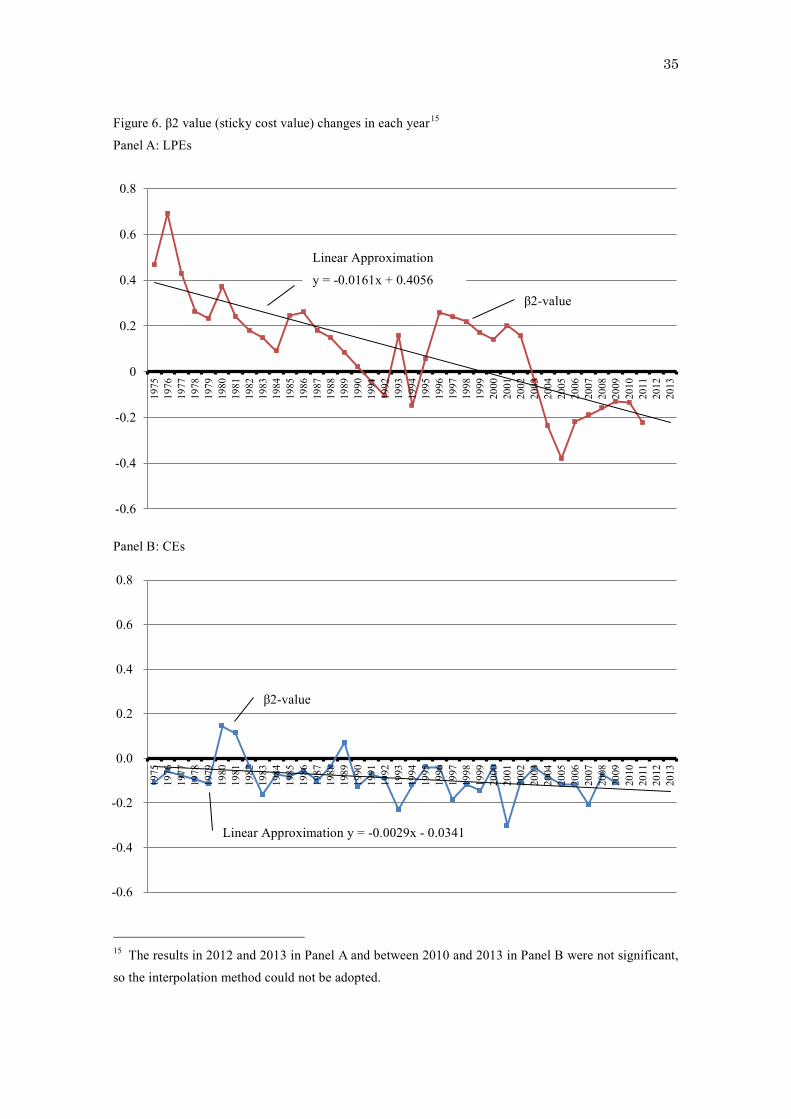
35

Figure 6. β2 value (sticky cost value) changes in each year15

Panel A: LPEs

Panel B: CEs

15 The results in 2012 and 2013 in Panel A and between 2010 and 2013 in Panel B were not significant,

so the interpolation method could not be adopted.

-0.6

-0.4

-0.2

0

0.2

0.4

0.6

0.8

1975

1976

1977

1978

1979

1980

1981

1982

1983

1984

1985

1986

1987

1988

1989

1990

1991

1992

1993

1994

1995

1996

1997

1998

1999

2000

2001

2002

2003

2004

2005

2006

2007

2008

2009

2010

2011

2012

2013

Linear Approximation

y = -0.0161x + 0.4056

β2-value

-0.6

-0.4

-0.2

0.0

0.2

0.4

0.6

0.8

1975

1976

1977

1978

1979

1980

1981

1982

1983

1984

1985

1986

1987

1988

1989

1990

1991

1992

1993

1994

1995

1996

1997

1998

1999

2000

2001

2002

2003

2004

2005

2006

2007

2008

2009

2010

2011

2012

2013

Linear Approximation y = -0.0029x - 0.0341

β2-value

36

Figure 7. β2, β4, β6, and β8 value (sticky cost value) change in each 4-year period

-0.1000

-0.0500

0.0000

0.0500

0.1000

0.1500

1 year 2 year 3 year 4 year

LPEs CEs

37

Table 1. LPEs in selected countries

Country Number ofmunicipalities

Number ofLPEs*

Sectors of activities**

Austria 2,359 149 Electricity, gas, heating, public transport, water, sewerage, waste,telecommunications, public equipement, cemeteries, public areas, health

Belgium 589 243 Electricity, gas, communication networks, funding, economicdevelopment, water, waste, health, social care

Czech Republic 6,258 339 Public transport, electricity, gas, heating, water, waste

Denmark 275 224 Economic development, electricity, gas, heating, water, waste, publictransport, leisure, computing, housing

Estonia 247 224 Electricity, gas, water, housing, public transport, heating, health, socialservices, trade, waste

Finland 448 944 Economic development, energy, water, sewerage, waste, publictransport, ports, telecommunications

France 36,565 1,198Tourism, planning, housing, public transport, economic development,water, sewerage, waste, environment, leisure, culture,telecommunications, parking spaces

Germany 13,854 3,500 Energy, economic development, water, waste, public transport, publicequipment, housing, banks, telecommunications

Greece 900 1,116 Water, sewerage, culture, tourism, training, careers

Italy 8,101 963Regions: economic development, planning, public equipment, publictransport, Provinces: commercial events, tourism municipalities: energy,water, waste, pharmacies, cemeteries

Japan 1,727 9,379Residential water, industrial water, transport, electricity, gas, hospitals,and other businesses that are run by each local government accordingto its own rules

Latvia 547 669Health, heating, waste, real estate operations, sport, public transport,pharmacies, water, social care, radio & TV, auditing, training, tourism,electricity

New Zealand 85 257 -

Poland 2,489 2,415 Water, construction, waste, real estate operations, electricity, gas,heating, public transport, trade, leisure, culture, sport

Portugal 4,037 76 Energy, public transport, tourism, environment, planning, commercialand industrial infrastructures, health, education, food industry

Slovakia 2,920 239 Waste, water, sewerage, heating, public spaces, health, public transport,public lighting, sport, housing, cemeteries, local television, tourism

Slovenia 193 60 Water, waste, road, cemeteries, public transport, public spaces,electricity, heating

South Korea 232 306 -

Spain 8,106 770 Municipalities and provinces: public transport, water, real estate,planning, economic development, cemeteries

Sweden 290 1,750 Energy, water, waste, public transport, housing, tourism, economicdevelopment

United Kingdom 326 185 Economic development, tourism,public equipment, health, social care

Created with reference to Saussier and Klien (2013)* LPEs include not only corporatized LPEs but also directly managed LPEs.** Sources: Dexia Crediop (2004)

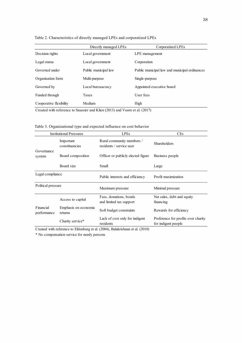
38

Table 2. Characteristics of directly managed LPEs and corporatized LPEs

Table 3. Organizational type and expected influence on cost behavior

Directly managed LPEs Corporatized LPEs

Decision rights Local government LPE management

Legal status Local government Corporation

Governed under Public municipal law Public municipal law and municipal ordinances

Organisation form Multi-purpose Single-purpose

Governed by Local bureaucracy Appointed executive board

Funded through Taxes User fees

Cooperative flexibility Medium High

Created with reference to Saussier and Klien (2013) and Voorn et al. (2017)

LPEs CEs

Importantconstituencies

Rural community members /residents / service user Shareholders

Board composition Officer or publicly elected figure Business people

Board size Small Large

Public interests and efficiency Profit maximization

Maximum pressure Minimal pressure

Access to capitalFees, donations, bondsand limited tax support

Net sales, debt and equityfinancing

Emphasis on economicreturns Soft budget constraints Rewards for efficiency

Charity service*Lack of cost only for indigentresidents

Preference for profits over charityfor indigent people

Created with reference to Eldenburg et al. (2004), Balakrishnan et al. (2010)* No compensation service for needy persons

Institutional Pressures

Governancesystem

Legal compliance

Political pressure

Financialperformance

39

Table 4. Descriptive statistics

Panel A: LPEs

Mean Standarddeviation

Minimum Lowerquartile

Median Upperquartile

Maximum SampleSize

Cost * 1,946,197 7,320,193 382 148,701 441,239 1,512,568 295,467,927Revenue ** 2,083,008 9,354,756 75 170,870 477,245 1,547,037 355,330,535Ln costt / costt-1 0.04101 0.09656 -0.48719 -0.00904 0.02957 0.08073 0.57912Ln revenuet / revenuet-1 0.04341 0.10744 -0.56932 -0.00933 0.02114 0.07433 0.66314Cost * 1,065,668 6,774,393 2,160 107,613 221,621 603,446 295,467,927Revenue ** 1,300,173 8,365,265 294 130,266 272,108 735,249 355,330,535Ln costt / costt-1 0.04577 0.10358 -0.48290 -0.01010 0.03116 0.08902 0.57874Ln revenuet / revenuet-1 0.04900 0.11070 -0.56601 -0.00895 0.02035 0.07403 0.66286Cost * 476,548 889,671 1,677 62,770 214,673 463,819 8,042,787Revenue ** 611,846 1,125,119 708 67,160 265,268 615,598 11,326,896Ln costt / costt-1 0.01980 0.11230 -0.48719 -0.03042 0.01117 0.06390 0.56784Ln revenuet / revenuet-1 0.02361 0.10851 -0.56583 -0.00629 0.00177 0.03059 0.64851Cost* 5,322,071 18,203,066 1,086 201,342 682,454 2,744,434 225,035,329Revenue** 7,300,351 28,571,454 75 101,462 555,047 3,217,774 344,008,013Ln costt / costt-1 0.03273 0.08959 -0.47635 -0.00871 0.01830 0.05856 0.57912Ln revenuet / revenuet-1 0.04654 0.10907 -0.55551 -0.00635 0.02001 0.07392 0.66314Cost * 8,925,017 19,250,696 382 348,485 1,779,477 6,132,778 149,541,551Revenue ** 8,705,197 21,195,366 1,741 306,571 1,570,819 5,174,318 163,824,708Ln costt / costt-1 0.01174 0.08491 -0.48158 -0.02899 0.01153 0.04929 0.57121Ln revenuet / revenuet-1 0.01463 0.09550 -0.53314 -0.02770 0.00457 0.04682 0.65543Cost * 1,685,005 1,401,034 7,198 715,088 1,359,032 2,324,393 7,926,889Revenue ** 2,265,455 1,792,677 13,700 948,625 1,911,831 3,179,656 9,605,919Ln costt / costt-1 0.03174 0.07822 -0.40621 -0.01232 0.02570 0.06965 0.45241Ln revenuet / revenuet-1 0.02399 0.07932 -0.37420 -0.01410 0.00869 0.04683 0.62548Cost * 1,263,644 3,293,313 27,840 198,447 447,234 954,152 40,287,262Revenue ** 1,377,663 3,505,486 27,253 215,862 487,177 1,064,206 40,270,247Ln costt / costt-1 0.04504 0.09517 -0.36607 -0.01443 0.02992 0.09005 0.56286Ln revenuet / revenuet-1 0.04829 0.09993 -0.28446 -0.01263 0.02464 0.08038 0.58733Cost * 3,090,634 3,621,221 28,828 726,049 1,687,856 4,030,324 31,602,391Revenue ** 2,790,521 3,360,561 700 621,644 1,463,985 3,637,399 32,298,365Ln costt / costt-1 0.04084 0.07661 -0.47925 -0.00031 0.03384 0.07567 0.57704Ln revenuet / revenuet-1 0.04011 0.10112 -0.56932 -0.00902 0.03386 0.08350 0.65367Cost * 1,900,347 3,679,698 42,733 235,815 496,231 1,091,269 16,949,597Revenue ** 1,718,437 3,206,354 58,783 188,243 477,556 1,372,835 14,497,486Ln costt / costt-1 0.01971 0.07123 -0.41089 -0.01870 0.01412 0.05088 0.43474Ln revenuet / revenuet-1 0.01658 0.06003 -0.42070 -0.01496 0.00482 0.03430 0.51378Cost * 497,635 481,220 22,252 195,702 290,347 642,219 2,372,781Revenue ** 692,079 884,575 22,778 186,634 342,516 826,008 4,569,640Ln costt / costt-1 0.02885 0.13502 -0.39079 -0.03376 0.02208 0.08266 0.53742Ln revenuet / revenuet-1 0.02526 0.15362 -0.56601 -0.03861 0.02085 0.07889 0.62754Cost * 82,441 68,813 2,222 38,621 74,155 108,933 372,239Revenue ** 127,903 112,924 4,366 51,008 98,883 174,920 563,130Ln costt / costt-1 0.00743 0.13908 -0.44680 -0.05085 0.00225 0.05782 0.57128Ln revenuet / revenuet-1 0.00069 0.12528 -0.53474 -0.04949 0.00000 0.05577 0.66278

* Operating expenses, ** Operating revenues

(Scale: 1,000 Yen)

Total

Residentialwatersupply

Industrialwatersupply

Sewerage

Transportation

Electricpower

Gas power

Hospitals

Wholesalemarket

Toll road

Car parking

115,929

64,675

7,296

4,525

2,677

369

1,261

2,274

32,066

516

270

40

Panel B: CEs

Mean Standarddeviation

Minimum Lowerquartile

Median Upperquartile

Maximum SampleSize

Cost * 125,774 648,568 2 9,127 23,643 68,737 21,359,227Revenue ** 131,521 659,166 3 9,817 24,978 72,599 21,403,613Ln costt / costt-1 0.03958 0.14110 -0.73556 -0.02781 0.03373 -0.03163 0.81494Ln revenuet / revenuet-1 0.03871 0.15540 -0.77351 0.10157 0.03435 0.10635 0.85349Cost * 94,881 152,120 2 4,295 17,998 138,252 602,390Revenue ** 96,747 153,914 3 4,419 20,480 140,481 612,888Ln costt / costt-1 0.03889 0.16101 -0.58739 -0.03284 0.02816 0.08908 0.73166Ln revenuet / revenuet-1 0.03931 0.18943 -0.70995 -0.03497 0.02480 0.09267 0.81866Cost * 60,597 22,065 261 52,866 67,054 74,242 101,943Revenue ** 62,770 22,779 180 55,544 68,566 76,659 104,996Ln costt / costt-1 0.03611 0.17392 -0.64688 -0.05549 0.02399 0.10066 0.58887Ln revenuet / revenuet-1 0.03559 0.19552 -0.64940 -0.06487 0.02476 0.09957 0.65909Cost * 57,586 53,898 2,769 10,215 55,354 72,511 218,544Revenue ** 76,792 94,113 4,638 15,943 60,555 84,634 452,228Ln costt / costt-1 0.04612 0.20656 -0.35237 -0.05296 0.02296 0.13136 0.80511Ln revenuet / revenuet-1 0.03331 0.23462 -0.66545 -0.08351 0.03760 0.14985 0.75472Cost * 132,019 237,300 174 21,094 47,333 132,397 2,015,551Revenue ** 136,941 246,680 212 21,748 49,045 135,420 2,168,285Ln costt / costt-1 0.02690 0.13266 -0.67110 -0.04520 0.02896 0.10185 0.68698Ln revenuet / revenuet-1 0.02572 0.13736 -0.74256 -0.04859 0.02892 0.10341 0.75482Cost * 72,220 212,318 27 5,542 16,471 56,063 3,464,264Revenue ** 75,446 220,709 22 6,162 17,553 59,375 3,480,490Ln costt / costt-1 0.06045 0.15442 -0.72516 -0.01157 0.03919 0.11229 0.81494Ln revenuet / revenuet-1 0.06093 0.16605 -0.76474 -0.01254 0.03795 0.11462 0.85105Cost * 43,365 100,497 16 3,610 10,185 31,938 1,045,802Revenue ** 45,521 105,242 7 3,923 10,908 33,395 1,100,228Ln costt / costt-1 0.05120 0.17111 -0.71247 -0.03426 0.03310 0.11877 0.79249Ln revenuet / revenuet-1 0.05190 0.18957 -0.77349 -0.03882 0.03393 0.12721 0.84832Cost * 60,838 122,718 41 7,817 19,003 54,036 1,563,564Revenue ** 66,040 131,944 10 8,578 20,478 58,024 1,602,062Ln costt / costt-1 0.04384 0.12206 -0.70580 -0.01651 0.03451 0.09264 0.80315Ln revenuet / revenuet-1 0.04249 0.13302 -0.73760 -0.01987 0.03496 0.09632 0.85053Cost * 100,727 294,103 158 9,626 22,143 70,419 3,678,713Revenue ** 105,601 306,000 236 10,254 23,420 73,837 3,753,397Ln costt / costt-1 0.02205 0.13031 -0.72685 -0.04353 0.02438 0.08901 0.78846Ln revenuet / revenuet-1 0.02044 0.14584 -0.77351 -0.05065 0.02428 0.09562 0.82038Cost * 97,397 374,006 10 8,861 19,449 49,936 4,862,221Revenue ** 101,324 382,156 21 9,415 20,626 52,640 4,994,719Ln costt / costt-1 0.03525 0.15359 -0.73094 -0.04333 0.03814 0.11601 0.80750Ln revenuet / revenuet-1 0.03442 0.18155 -0.77308 -0.05260 0.04087 0.12769 0.85349Cost * 136,215 531,671 23 11,284 26,030 63,670 10,970,663Revenue ** 141,568 554,663 6 12,113 27,180 66,138 12,079,264Ln costt / costt-1 0.03515 0.13022 -0.73524 -0.02943 0.03336 0.09610 0.81312Ln revenuet / revenuet-1 0.03423 0.14288 -0.76523 -0.03243 0.03415 0.09974 0.84630Cost * 363,828 1,715,798 75 18,530 59,053 147,589 21,359,227Revenue ** 369,269 1,720,356 51 20,414 61,312 152,949 21,403,613Ln costt / costt-1 0.04457 0.15367 -0.73556 -0.02835 0.03425 0.11203 0.81210Ln revenuet / revenuet-1 0.04371 0.16007 -0.75328 -0.03005 0.03524 0.11322 0.83715Cost * 118,766 383,299 101 9,540 24,001 63,343 6,034,976Revenue ** 132,210 435,412 94 10,141 25,172 67,917 6,371,287Ln costt / costt-1 0.04143 0.12023 -0.71695 -0.01427 0.03405 0.09108 0.80006Ln revenuet / revenuet-1 0.04007 0.12611 -0.73672 -0.01583 0.03397 0.09146 0.83182

* Operating expenses, ** Operating revenues

(Scale: 1,000,000 Yen)

Agriculture andfishery

Mining

Petroleum

Total

Foods

Chemicals

Resources andmaterials

Machinery andelectric machinery

Automobiles andtransportation

equipment

Financial

Construction

Tectiles, pulp andpaper

10,279

8,040

14,947

11,402

Broadcasting,software,

commercial etc.

8,920

11,944

6,679

6,287

84,343

426

82

65

5,272

41

Table 5. Cost behavior based on the panel data analysis using model 1

Panel A: LPEs

Panel B: CEs

0.0200 *** 0.0207 *** 0.0200 ***

67.38 68.24 67.20

＋ 0.5077 *** 0.4952 *** 0.5077 ***

195.84 183.96 195.33

－ 0.0677 *** 0.0791 *** 0.0677 ***

9.74 10.69 9.71

Statistic (Degree of freedom) P-value

393.42 (2) 0H-Test

N

DW

Adj.R2

2.1138 2.1819 2.1138

0.3389

115,929 115,929

β0

β1

β 2

Predictedsign

0.3355 0.3389

115,929

Randomeffects

FixedeffectsPooled

0.0023 *** 0.0026 *** 0.0028 ***

8.49 9.23 7.44

＋ 0.8704 *** 0.8647 *** 0.8682 ***

463.94 413.83 448.82

－ -0.1008 *** -0.0978 *** -0.1045 ***

-28.85 -24.92 -28.74

Statistic (Degree of freedom) P-value

20.48 (2) 0

For β0, β1, and β2, upper data indicate coefficient estimates;

lower data indicate t-statistics, *significant at the 10% level,

**significant at the 5% level, ***significant at the 1% level,

Adj.R2=Adjusted R2, N=Number of Observations,

DW=Durbin-Watson ratio, H-Test=HausmanTest,

β2 indicates the value of the sticky or anti-sticky costs.

84,343

Adj.R2

N

PooledFixedeffects

Randomeffects

1.6913

0.8467 0.8337

1.6487

0.8379

84,343

DW

H-Test

1.8114

84,343

Predictedsign

β0

β1

β 2

42

Table 6. The results for individual years based on OLS analysis using model 1

Panel A: LPEs Year Adj.R2 N F-statistic1975 0.0834 *** 0.2884 *** 0.4668 *** 0.2751 2,656 504.75 0

1976 0.0864 *** 0.2572 *** 0.6934 *** 0.2730 2,723 512.00 0

1977 0.0860 *** 0.3476 *** 0.4302 *** 0.2701 2,802 519.33 0

1978 0.0528 *** 0.3991 *** 0.2634 *** 0.2763 2,858 546.30 0

1979 0.0667 *** 0.4025 *** 0.2336 *** 0.2648 2,886 520.66 0

1980 0.0916 *** 0.3922 *** 0.3728 *** 0.3513 2,890 783.28 0

1981 0.0476 *** 0.3327 *** 0.2413 *** 0.2548 2,934 502.45 0

1982 0.0255 *** 0.3887 *** 0.1806 *** 0.2594 2,962 519.64 0

1983 0.0246 *** 0.4699 *** 0.1482 *** 0.2988 2,991 637.99 0

1984 0.0297 *** 0.4181 *** 0.0902 * 0.2515 3,028 509.42 0

1985 0.0317 *** 0.4139 *** 0.2455 *** 0.2602 3,050 537.21 0

1986 0.0197 *** 0.4338 *** 0.2608 *** 0.2680 3,075 563.78 0

1987 0.0143 *** 0.5593 *** 0.1810 *** 0.3488 3,080 825.59 0

1988 0.0242 *** 0.5104 *** 0.1485 *** 0.2868 3,110 626.03 0

1989 0.0243 *** 0.5686 *** 0.0430 0.3046 3,119 683.80 0

1990 0.0384 *** 0.5471 *** -0.0170 0.2625 3,130 557.86 0

1991 0.0400 *** 0.5447 *** 0.0765 0.2582 3,137 546.72 0

1992 0.0306 *** 0.5313 *** -0.1058 ** 0.2550 3,163 542.28 0

1993 0.0280 *** 0.5212 *** 0.1578 *** 0.2928 3,179 658.97 0

1994 0.0231 *** 0.4643 *** -0.1466 *** 0.1953 3,180 386.74 0

1995 0.0132 *** 0.5559 *** 0.0230 0.2637 3,200 573.78 0

1996 0.0130 *** 0.4663 *** 0.2584 *** 0.2767 3,204 613.60 0

1997 0.0156 *** 0.4735 *** 0.2397 *** 0.2874 3,218 649.59 0

1998 0.0105 *** 0.4898 *** 0.2175 *** 0.2764 3,219 615.49 0

1999 0.0091 *** 0.5487 *** 0.1725 *** 0.2742 3,230 610.90 0

2000 0.0049 *** 0.5338 *** 0.1411 *** 0.2718 3,218 601.34 0

2001 0.0114 *** 0.4594 *** 0.2003 *** 0.2171 3,224 447.96 0

2002 -0.0038 ** 0.4173 *** 0.1568 *** 0.2193 3,232 454.84 0

2003 -0.0032 ** 0.5785 *** -0.0134 0.2736 3,198 602.98 0

2004 -0.0028 * 0.6758 *** -0.2361 *** 0.3058 2,821 622.12 0

2005 -0.0025 0.8186 *** -0.3796 *** 0.4385 2,454 958.94 0

2006 0.0017 0.5754 *** -0.2197 *** 0.1988 2,725 338.93 0

2007 0.0032 ** 0.4978 *** 0.0439 0.2448 2,708 439.79 0

2008 0.0033 ** 0.4470 *** -0.0240 0.2427 2,710 435.20 0

2009 -0.0040 *** 0.5068 *** -0.1284 *** 0.2081 2,698 355.35 0

2010 -0.0040 *** 0.4387 *** -0.1333 *** 0.1414 2,723 225.06 0

2011 0.0052 *** 0.5021 *** -0.2221 *** 0.1472 2,687 232.87 0

2012 0.0061 *** 0.3067 *** 0.0309 0.1048 2,740 161.25 0

2013 0.0085 *** 0.3630 *** -0.0593 0.0799 2,767 121.07 0

*significant at the 10% level, **significant at the 5% level, ***significant at the 1% level, Adj.R2=Adjusted R2, N=Number of Observations

β０ β１ β２Prob(F-statistic)

43

Panel B: CEs

Year β０ β１ β２ Adj.R2 N F-statistic

1975 0.0298 *** 0.8926 *** -0.1076 *** 0.9298 1,053 6,966.39 0

1976 0.0168 *** 0.8543 *** -0.0567 ** 0.9092 1,065 5,330.40 0

1977 0.0123 *** 0.8500 *** -0.0206 0.9236 1,090 6,579.05 0

1978 0.0119 *** 0.9113 *** 0.0097 0.9332 1,149 8,025.62 0

1979 -0.0017 0.9397 *** -0.1150 *** 0.9321 1,367 9,374.25 0

1980 0.0069 *** 0.9050 *** 0.1452 *** 0.9241 1,385 8,428.48 0

1981 0.0137 *** 0.8879 *** 0.1137 *** 0.9383 1,406 10,678.92 0

1982 0.0096 *** 0.9295 *** -0.0363 * 0.9400 1,436 11,249.80 0

1983 0.0059 *** 0.9583 *** -0.1630 *** 0.9342 1,479 10,497.84 0

1984 0.0033 *** 0.9371 *** -0.0730 *** 0.9509 1,525 14,756.17 0

1985 0.0024 ** 0.9439 *** -0.0812 *** 0.9506 1,575 15,138.00 0

1986 0.0065 *** 0.9357 *** -0.0535 *** 0.9432 1,621 13,444.14 0

1987 0.0014 0.9704 *** -0.0997 *** 0.9364 1,673 12,319.27 0

1988 -0.0027 ** 0.9274 *** -0.0356 * 0.9156 1,720 9,322.80 0

1989 0.0035 *** 0.8948 *** 0.0722 *** 0.9404 1,759 13,874.49 0

1990 0.0040 *** 0.9445 *** -0.1287 *** 0.9125 1,837 9,573.52 0

1991 0.0073 *** 0.9377 *** -0.0722 *** 0.9292 1,916 12,558.01 0

1992 0.0062 *** 0.9458 *** -0.0883 *** 0.9367 1,981 14,654.93 0

1993 0.0007 0.9829 *** -0.2312 *** 0.9381 2,053 15,552.19 0

1994 -0.0014 0.9539 *** -0.1195 *** 0.9304 2,107 14,068.74 0

1995 -0.0025 *** 0.9156 *** -0.0387 *** 0.9294 2,150 14,142.35 0

1996 0.0009 0.9173 *** -0.0425 ** 0.9256 2,214 13,765.34 0

1997 -0.0018 * 0.9506 *** -0.1833 *** 0.9018 2,320 10,654.80 0

1998 0.0023 *** 0.9527 *** -0.1180 *** 0.9396 2,398 18,638.26 0

1999 -0.0095 *** 0.9371 *** -0.1462 *** 0.9215 2,487 14,597.35 0

2000 -0.0055 *** 0.9057 *** -0.0351 ** 0.8997 2,554 11,446.83 0

2001 -0.0052 *** 0.9058 *** -0.3004 *** 0.8385 2,637 6,845.25 0

2002 0.0021 0.8670 *** -0.1067 *** 0.8690 2,730 9,054.03 0

2003 -0.0057 0.8663 *** -0.0434 ** 0.8287 2,869 6,938.02 0

2004 -0.0005 0.8287 *** 0.0063 0.8195 2,929 6,647.12 0

2005 0.0023 0.8583 *** -0.1164 *** 0.8104 2,963 6,331.68 0

2006 0.0044 *** 0.8663 *** -0.1177 *** 0.8128 2,974 6,456.73 0

2007 0.0056 *** 0.8797 *** -0.2054 *** 0.7544 3,007 4,617.78 0

2008 0.0120 *** 0.7870 *** -0.0728 *** 0.6937 3,054 3,457.98 0

2009 0.0061 *** 0.8248 *** -0.1069 *** 0.7444 3,098 4,511.85 0

2010 -0.0211 *** 0.7556 *** -0.0237 0.7156 3,112 3,914.58 0

2011 -0.0009 0.7059 *** -0.0111 0.6902 3,183 3,545.08 0

2012 0.0064 *** 0.6528 *** 0.0077 0.6426 3,206 2,881.67 0

2013 0.0012 0.7256 *** -0.0174 0.6940 3,261 3,698.40 0

*significant at the 10% level, **significant at the 5% level, ***significant at the 1% level, Adj.R2=Adjusted R2, N=Number of Observations

Prob(F-statistic)

44

Table 7. Cost behavior of each industry based on the panel data analysis using model 1

Panel A: LPEs

0.02

54**

*0.

0261

***

0.02

54**

*0.

0135

***

0.01

35**

*0.

0135

***

0.00

98**

*0.

0107

***

0.01

00**

*0.

0065

***

0.00

73**

*0.

0065

***

59.1

759

.80

58.8

59.

409.

219.

366.

717.

246.

053.

543.

943.

540.

4820

***

0.47

19**

*0.

4820

***

0.31

11**

*0.

3101

***

0.31

11**

*0.

4224

***

0.40

59**

*0.

4179

***

0.43

22**

*0.

4159

***

0.43

22**

*

137.

7813

1.64

137.

0322

.33

21.4

422

.23

33.7

131

.17

33.1

820

.75

19.2

720

.72

0.27

48**

*0.

2908

***

0.27

48**

*0.

0565

*0.

0500

0.05

65*

-0.2

731

***

-0.2

656

***

-0.2

713

***

0.04

280.

0693

*0.

0428

23.8

224

.29

23.6

91.

831.

561.

83-7

.63

-7.2

7-7

.58

1.07

1.66

1.07

H-te

st

0.01

65**

*0.

0168

***

0.01

65**

*0.

0170

***

0.01

74**

*0.

0170

***

0.01

27**

*0.

0128

***

0.01

27**

*0.

0134

***

0.01

35**

*0.

0134

***

6.76

6.79

6.70

9.50

9.61

9.42

33.6

933

.33

33.6

63.

873.

883.

850.

5541

***

0.54

76**

*0.

5541

***

0.67

76**

*0.

6705

***

0.67

76**

*0.

6315

***

0.62

79**

*0.

6315

***

0.54

07**

*0.

5297

***

0.54

07**

*

19.2

418

.55

19.0

645

.03

43.6

244

.67

170.

8416

6.43

170.

719.

499.

149.

45-0

.147

3*

-0.1

326

-0.1

473

*0.

3908

***

0.39

96**

*0.

3908

***

-0.1

581

***

-0.1

640

***

-0.1

581

***

0.25

06*

0.24

64*

0.25

06*

-1.8

3-1

.60

-1.8

16.

566.

566.

50-2

0.34

-20.

38-2

0.33

1.85

1.80

1.85

H-te

st

0.01

310.

0138

0.01

31-0

.019

7**

-0.0

215

**-0

.019

7**

1.33

1.37

1.31

-2.2

7-2

.44

-2.2

60.

4400

***

0.43

16**

*0.

4400

***

0.71

01**

*0.

7247

***

0.71

01**

*

6.18

5.90

6.12

8.28

8.28

8.25

-0.1

208

-0.1

073

-0.1

208

-0.6

605

***

-0.7

056

***

-0.6

605

***

-0.9

2-0

.79

-0.9

1-4

.75

-4.9

4-4

.74

H-te

st

Upp

er d

ata

indi

cate

coe

ffic

ient

est

imat

es; l

ower

dat

a in

dica

te t-

stat

istic

s, *:

sign

ifica

nt a

t the

10%

leve

l, **

: sig

nific

ant a

t the

5%

leve

l, **

*: si

gnifi

cant

at t

he 1

% le

vel,

Adj

.R2 =A

djus

ted

R2 , N

=Num

ber o

f Obs

erva

tions

, DW

=Dur

bin-

Wat

son

ratio

, H-T

est:H

ausm

an T

est,

β2 in

dica

tes t

he v

alue

of t

he st

icky

or a

nti-s

ticky

cos

ts.

Car

par

king

Toll　

road

β 0

Ran

dom

Fixe

dPo

oled

Ran

dom

Fixe

dPo

oled

0.16

900.

1646

0.16

900.

1951

0.17

810.

1951

Adj

.R2

β2β 1 DW

369

369

369

270

270

270

N

0.35

(2)

2.10

0.81

(2)

0.42

2.22

952.

2731

2.22

951.

7790

1.78

831.

7790

Res

iden

tial w

ater

supp

lyIn

dust

rial w

ater

supp

lySe

wag

ePo

oled

Fixe

dR

ando

mPo

oled

Tran

spor

tatio

nPo

oled

Fixe

dR

ando

m

Elec

tric

pow

erFi

xed

Ran

dom

2.12

571.

8467

1.92

221.

8679

245.

02(2

)0.

001.

80

β 1 β2

Adj

.R2

0.31

890.

3115

0.31

89

Fixe

dR

ando

mPo

oled

β 0

0.10

040.

0927

0.10

040.

2180

Fixe

dR

ando

m

64,6

7564

,675

64,6

757,

296

7,29

67,

296

4,52

54,

525

4,52

52,

677

0.28

290.

2695

0.28

29

β 0 β 1 β2

Adj

.R2

0.25

63

8.62

(2)

0.00

0.23

040.

2120

(2)

0.41

2.20

752.

2369

2.20

752.

1257

2.17

46

Pool

ed

16.1

8

0.25

450.

2563

DWN

2,67

72,

677

2.06

602.

0214

2.43

86D

W

2.02

14

N1,

261

1,26

11,

261

2,27

42,

274

2,27

432

,066

32,0

6632

,066

516

516

516

1.64

(2)

0.44

Gas

pow

erH

ospi

tals

Who

lesa

le m

arke

tFi

xed

2.45

532.

4386

8.68

(2)

0.01

109.

05(2

)0.

001.

74(2

)1.

9436

1.90

192.

0174

2.04

482.

3302

0.42

2.01

742.

3448

0.01

0.59

580.

5892

0.59

580.

5960

0.59

540.

5960

0.26

220.

2556

Ran

dom

0.26

22

Pool

edFi

xed

Ran

dom

Pool

edFi

xed

Ran

dom

Pool

ed

2.33

021.

9019

(2)

45

Panel B: CEs

0.00

800.

0059

0.00

840.

0059

0.00

580.

0059

-0.0

109

0.00

49-0

.010

90.

0011

*0.

0012

**0.

0011

*

1.69

1.11

1.37

0.52

0.47

0.52

-0.4

60.

21-0

.49

1.87

2.02

1.85

0.76

06**

*0.

7735

***

0.75

39**

*0.

8134

***

0.81

32**

*0.

8134

***

0.85

12**

*0.

7625

***

0.85

12**

*0.

9576

***

0.95

63**

*0.

9576

***

28.4

222

.42

27.0

512

.79

11.4

212

.64

7.28

6.51

7.72

-3.6

819

6.60

205.

95-0

.024

4-0

.061

3-0

.020

2-0

.025

4-0

.028

9-0

.025

4-0

.424

9**

-0.2

344

-0.4

249

**-0

.030

6**

*-0

.028

3**

*-0

.030

8**

*

-0.4

7-0

.90

-0.3

7-0

.21

-0.2

1-0

.21

-2.0

7-1

.11

-2.2

0-3

.68

-3.1

8-3

.67

H-te

st

0.00

30**

0.00

41**

*0.

0040

***

0.00

32**

0.00

75**

*0.

0080

***

0.00

17**

0.00

30**

*0.

0030

***

0.00

23**

*0.

0021

***

0.00

21*

2.54

3.23

2.64

2.20

4.84

3.93

2.12

3.54

2.48

2.99

2.65

1.81

0.86

71**

*0.

8520

***

0.86

24**

*0.

8277

***

0.78

65**

*0.

8091

***

0.86

27**

*0.

8503

***

0.85

73**

*0.

8546

***

0.85

92**

*0.

8574

***

123.

7810

2.46

117.

6010

4.93

83.7

597

.56

135.

1512

1.25

130.

2913

8.10

136.

0313

8.79

-0.1

764

***

-0.1

697

***

-0.1

771

***

-0.1

247

***

-0.0

721

***

-0.1

092

***

-0.2

071

***

-0.1

780

***

-0.2

038

***

-0.0

535

***

-0.0

574

***

-0.0

610

***

-11.

41-9

.37

-10.

98-7

.75

-3.9

2-6

.56

-16.

13-1

2.44

-15.

37-5

.08

-5.2

2-5

.71

H-te

st

0.00

36**

*0.

0034

***

0.00

32**

*0.

0025

***

0.00

21**

*0.

0025

***

-0.0

009

-0.0

008

-0.0

008

0.00

10**

0.00

10*

0.00

10**

5.94

5.41

4.27

4.27

3.44

3.22

-0.9

7-0

.76

-0.7

51.

981.

751.

980.

8280

***

0.82

67**

*0.

8283

***

0.88

49**

*0.

8861

***

0.88

35**

*0.

9211

***

0.91

79**

*0.

9207

***

0.93

63**

*0.

9331

***

0.93

63**

*

219.

8920

0.41

215.

0419

7.99

182.

1719

3.04

143.

1212

7.14

140.

2921

8.09

198.

0521

8.04

-0.0

638

***

-0.0

676

***

-0.0

688

***

-0.0

695

***

-0.0

797

***

-0.0

739

***

-0.1

518

***

-0.1

515

***

-0.1

547

***

-0.1

186

***

-0.1

265

***

-0.1

186

***

-9.7

6-9

.31

-10.

18-8

.53

-8.8

2-8

.78

-12.

42-1

0.89

-12.

37-1

4.27

-13.

64-1

4.27

H-te

st

Upp

er d

ata

indi

cate

coe

ffic

ient

est

imat

es; l

ower

dat

a in

dica

te t-

stat

istic

s, *:

sign

ifica

nt a

t the

10%

leve

l, **

: sig

nific

ant a

t the

5%

leve

l, **

*: si

gnifi

cant

at t

he 1

% le

vel,

Adj

.R2 =A

djus

ted

R2 , N

=Num

ber o

f Obs

erva

tions

, DW

=Dur

bin-

Wat

son

ratio

, H-T

est:H

ausm

an T

est,

β2 in

dica

tes t

he v

alue

of t

he st

icky

or a

nti-s

ticky

cos

ts.

8,04

08,

040

14,9

4714

,947

14,9

4711

,402

11,4

0211

,402

8,92

08,

920

8,92

011

,944

11,9

4411

,944

1.86

291.

7186

14.2

2(2

)0.

0026

.63

(2)

1.73

611.

5495

1.50

55

Agr

icul

ture

and

fish

ery

Min

ing

Petro

leum

Con

stru

ctio

nPo

oled

Fixe

d

N42

642

642

682

8282

6565

655,

272

5,27

25,

272

Ran

dom

Pool

edFi

xed

Ran

dom

Ran

dom

Pool

edFi

xed

Ran

dom

Pool

edFi

xed

β 0 β 1 β2

Adj

.R2

0.78

180.

7885

0.77

510.

8112

0.80

680.

9556

DW

1.98

592.

1566

2.00

541.

6398

1.64

73

0.81

120.

5767

0.62

370.

5767

0.95

570.

9559

Res

ourc

es a

nd m

ater

ials

Pool

ed

9.74

(2)

0.01

0.90

(2)

0.64

2.03

961.

10(2

)0.

580.

19(2

)0.

911.

6398

2.13

312.

3279

2.13

312.

0352

2.10

86

Ran

dom

Pool

edFi

xed

Ran

dom

Fixe

dR

ando

mPo

oled

Fixe

dR

ando

mPo

oled

β 0 β 1 β2

Adj

.R2

0.77

470.

7851

0.76

270.

7578

Fixe

dFo

ods

Tect

iles,

pulp

and

pap

erC

hem

ical

s

0.87

280.

8638

DW

1.57

781.

7382

1.61

971.

4800

0.77

960.

7376

0.74

810.

7667

0.74

060.

8620

N6,

679

6,67

96,

679

6,28

76,

287

6,28

710

,279

10,2

7910

,279

8,04

01.

6892

1.56

481.

6629

0.00

Mac

hine

ry a

nd e

lect

ric m

achi

nery

Aut

omob

iles a

nd tr

ansp

orta

tion

equi

pmen

tFi

nanc

ial

Bro

adca

stin

g, s

oftw

are,

com

mer

cial

etc

.

0.00

35.1

0(2

)0.

0010

8.33

(2)

β 0 β 1 β2

Adj

.R2

0.89

200.

8961

Pool

edFi

xed

Ran

dom

Pool

edFi

xed

Ran

dom

Pool

edFi

xed

Ran

dom

Pool

edFi

xed

Ran

dom

0.80

800.

8793

0.87

920.

8793

0.89

130.

8829

0.88

850.

8806

0.81

120.

8143

1.79

431.

9776

2.03

491.

9776

DW

1.72

041.

8500

1.74

631.

6846

1.83

441.

7211

1.77

961.

8728

N

53.6

0(2

)0.

006.

44(2

)0.

043.

12(2

)0.

211.

54(2

)0.

46

46

Table 8. Population changes and cost behavior based on the panel data analysis using model 2

Panel A: LPEs

0.0041 *** 0.0041 *** 0.0041 *** 0.0041 *** 0.0041 *** 0.0041 ***

11.38 10.66 11.30 11.38 10.80 11.300.5321 *** 0.5227 *** 0.5321 *** 0.5321 *** 0.5212 *** 0.5321 ***

96.27 84.53 95.56 96.33 84.34 95.66-0.0347 *** -0.0401 *** -0.0347 *** 0.6357 *** 0.9987 *** 0.6357 ***

-3.57 -3.60 -3.54 7.44 9.89 7.39-0.4190 *** -0.3080 ** -0.4190 ***

-3.10 -2.17 -3.080.3372 *** 0.5216 *** 0.3372 ***

7.91 10.36 7.85

Statistic (Degree of freedom) P-value Statistic (Degree of freedom) P-value

56.96 0 102.74 0

The effect of youth (0-14 years) population change

PooledFixedeffects

Randomeffects

β5

β6

0.2465 0.2361

β0

β1

β2

β3

β 4

β 3

β4

β5

β6

β2

The effect of total population change

Fixedeffects

Randomeffects

β0

β1

Pooled

(3) (3)

DW 2.1745 2.3227 2.1745

H-Test

Adj.R2 0.2458

2.3250 2.1775

H-Test

2.1775

0.2465

N 55,976 55,976 55,976N

DW

0.2346 0.2458

55,976 55,976 55,976

Adj.R2

0.0041 *** 0.0041 *** 0.0041 *** 0.0042 *** 0.0041 *** 0.0041 ***

11.33 10.60 11.25 11.41 10.72 11.330.5322 *** 0.5227 *** 0.5322 *** 0.5320 *** 0.5224 *** 0.5322 ***

96.29 84.53 95.58 96.25 84.47 95.54-0.0329 -0.0861 * -0.0329 -0.1367 *** -0.1721 *** -0.1367 ***

-0.76 -1.67 -0.76 -3.48 -3.70 -3.45

0.0053 -0.0954 0.00530.06 -0.90 0.06

-0.0695 *** -0.0901 *** -0.0695 ***

-2.66 -2.91 -2.64

Statistic (Degree of freedom) P-value Statistic (Degree of freedom) P-value

57.83 0 56.72 0

From β0 to β6, upper data indicate coefficient estimates; lower data indicate t-statistics, *significant at the 10% level,

**significant at the 5% level, ***significant at the 1% level, Adj.R2=Adjusted R2, N=Number of Observations,

DW=Durbin-Watson ratio, H-Test=HausmanTest, β3 means Pop_total, β4 means Pop_youth, β5 means Pop_middle and β6 means Pop_elder

DW 2.1768 2.3246 2.1768

H-Test

0.2458

N 55,976 55,976 55,976

β5

β 6

β2

β3

β4

N 55,976 55,976 55,976

β 5

The effect of elderly (65+ years) population change

PooledFixedeffects

Randomeffects

2.1768

β0

β1

β2

β3

β4

Adj.R2 0.2458 0.2346

β0

β1

The effect of middle-aged (15-64 years) population change

PooledFixedeffects

Randomeffects

0.2457

β6

Adj.R2 0.2457 0.2345

(3)H-Test

DW 2.1768 2.3245

(3)

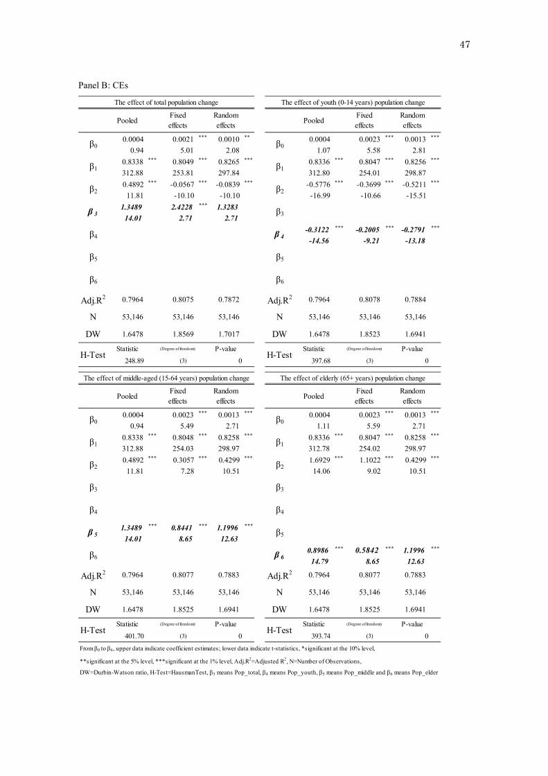
47

Panel B: CEs

0.0004 0.0021 *** 0.0010 ** 0.0004 0.0023 *** 0.0013 ***

0.94 5.01 2.08 1.07 5.58 2.810.8338 *** 0.8049 *** 0.8265 *** 0.8336 *** 0.8047 *** 0.8256 ***

312.88 253.81 297.84 312.80 254.01 298.870.4892 *** -0.0567 *** -0.0839 *** -0.5776 *** -0.3699 *** -0.5211 ***

11.81 -10.10 -10.10 -16.99 -10.66 -15.511.3489 2.4228 *** 1.328314.01 2.71 2.71

-0.3122 *** -0.2005 *** -0.2791 ***

-14.56 -9.21 -13.18

Statistic (Degree of freedom) P-value Statistic (Degree of freedom) P-value

248.89 0 397.68 0H-Test H-Test

DW 1.6478 1.8569 1.7017 DW 1.6478 1.8523 1.6941

N 53,146 53,146 53,146 N 53,146 53,146 53,146

Adj.R2 0.7964 0.8075 0.7872 Adj.R2

β5 β5

0.7964 0.8078 0.7884

β6 β6

β 3 β3

β4 β 4

β2 β2

PooledFixedeffects

Randomeffects

β1 β1

PooledFixedeffects

Randomeffects

β0 β0

The effect of total population change The effect of youth (0-14 years) population change

(3) (3)

0.0004 0.0023 *** 0.0013 *** 0.0004 0.0023 *** 0.0013 ***

0.94 5.49 2.71 1.11 5.59 2.710.8338 *** 0.8048 *** 0.8258 *** 0.8336 *** 0.8047 *** 0.8258 ***

312.88 254.03 298.97 312.78 254.02 298.970.4892 *** 0.3057 *** 0.4299 *** 1.6929 *** 1.1022 *** 0.4299 ***

11.81 7.28 10.51 14.06 9.02 10.51

1.3489 *** 0.8441 *** 1.1996 ***

14.01 8.65 12.630.8986 *** 0.5842 *** 1.1996 ***

14.79 8.65 12.63

Statistic (Degree of freedom) P-value Statistic (Degree of freedom) P-value

401.70 0 393.74 0

From β0 to β6, upper data indicate coefficient estimates; lower data indicate t-statistics, *significant at the 10% level,

**significant at the 5% level, ***significant at the 1% level, Adj.R2=Adjusted R2, N=Number of Observations,

DW=Durbin-Watson ratio, H-Test=HausmanTest, β3 means Pop_total, β4 means Pop_youth, β5 means Pop_middle and β6 means Pop_elder

1.6941

H-Test H-Test

53,146

DW 1.6478 1.8525 1.6941 DW 1.6478 1.8525

(3)

53,146 N 53,146 53,146

0.8077 0.7883 Adj.R2 0.7964 0.8077

N

β 5

0.7883

β5

β6 β 6

β3 β3

β0

Fixedeffects

Randomeffects

β4 β4

β2 β2

PooledFixedeffectsPooled

β1 β1

Randomeffects

β0

The effect of middle-aged (15-64 years) population change The effect of elderly (65+ years) population change

(3)

Adj.R2 0.7964

53,146 53,146

48

Table 9. Cost behavior over 4 years based on the panel data analysis using model 3

β0 0.0113 *** 0.0122 *** 0.0113 *** 0.0010 *** 0.0015 *** 0.0011 ***

31.30 30.76 31.10 4.03 4.45 3.78

β1 0.4764 *** 0.4693 *** 0.4764 *** 0.8748 *** 0.8760 *** 0.8744 ***

141.08 135.29 140.16 442.75 428.33 444.22

β 2 0.0972 *** 0.1157 *** 0.0972 *** -0.0719 *** -0.0685 *** -0.0714 ***

(t/t-1) 12.26 13.89 12.18 -21.40 -19.31 -21.22β3 0.0586 *** 0.0550 *** 0.0586 *** 0.0352 *** 0.0346 *** 0.0349 ***

18.74 17.18 18.62 18.09 17.41 18.07

β 4 0.0137 * 0.0226 *** 0.0137 * 0.0470 *** 0.0505 *** 0.0474 ***

(t-1/t-2) 1.74 2.76 1.73 13.72 14.23 13.90β5 0.0710 *** 0.0690 *** 0.0710 *** 0.0229 *** 0.0213 *** 0.0226 ***

24.95 23.75 24.78 12.25 11.15 12.18

β 6 -0.0226 *** -0.0179 ** -0.0226 *** 0.0216 *** 0.0244 *** 0.0217 ***

(t-2/t-3) -2.94 -2.23 -2.92 6.44 7.02 6.50β7 0.0460 *** 0.0456 *** 0.0460 *** 0.0224 *** 0.0217 *** 0.0221 ***

18.13 17.58 18.01 13.52 12.45 13.40

β 8 -0.0156 ** -0.0158 ** -0.0156 ** -0.0075 ** -0.0070 ** -0.0076 **

(t-3/t-4) -2.15 -2.09 -2.13 -2.40 -2.12 -2.44Adj.R2 0.3194 0.3104 0.3194 0.8926 0.8956 0.8904

N 100,923 100,923 100,923 72,814 72,814 72,814DW 2.1958 2.2610 2.1958 1.9671 2.1173 1.9863

Statistic (Degree of freedom) P-value Statistic (Degree of freedom) P-value138.30 (8) 0 285.45 (8) 0

From β0 to β8, upper data indicate coefficient estimates; lower data indicate t-statistics,*significant at the 10% level, **significant at the 5% level, ***significant at the 1% level

Adj.R2=Adjusted R2, N=Number of Observations, DW=Durbin-Watson ratio, H-Test=HausmanTest,β2 value is the rate of change from t-1 to t, β4, β6, and β8 values represented the annual change in asymmetric cost behavior for t-1/t-2, t-2/t-3, and t-3/t-4, respectively.

H-Test

Pooled Fixedeffects

Randomeffects

Panel B: CEsPanel A: LPEs

Pooled Fixedeffects

Randomeffects