TRA NSPORTA TION R ESEARCH RECORD 1215 31

Cost Allocation Implications of Flexible Pavement Deterioration Models

L. R. RILETT, B. G. HUTCHINSON, AND R. C. G. HAAS

This paper explores the implications of flexible pavement dete­rioration models that allow the separation of highway pave­ment life-cycle costs into joint and common costs and the allo­cation of the joint costs to various vehicle classes on the basis of their pavement damage characteristics. The Ontario flexible pavement deterioration model is used to calculate the joint and common cost portions of pavement costs for a range of traffic loadings and pavement strategies. These calculations show that the portion of pavement costs attributed to traffic varied from one-quarter to one-third, with the remainder being attributed to environmental degradation. The analyses show that there are substantial economics of scale with respect to traffic load­ings and that joint costs per ESAL-kilometcr decreased sig­nificantly with increased traffic loadings. Large differences in the joint costs per vehicle-kilometer occur between the different truck types, while the joint costs per tonne-kilometer are more uniform. The main weakness of the Ontario model seems to be in the prediction of the performance of overlaid pavements.

Public policy makers and their advisors have addressed the problem of the equitable allocation of the costs of providing highway service to various types of users for some 30 years. The principal emphasis has been on the allocation of pave­ment costs, although bridge and traffic capacity costs have been examined in recent years.

Wong and Markow (J) have listed three equity concepts that might be used as a basis for the pricing of highway services:

1. The received benefit-equity concept where user charges are proportional to the benefits received by users;

2. The occasioned cost equity concept where costs are assigned to users on the basis of the costs occasioned by each class of user; and

3. A method that assigns costs on the basis of the ability to pay of each class of user.

The most commonly accepted method is the cost­occasioned approach in which various types of users are assigned the average costs to the highway agency of their trips. The challenge with this approach is to identify a relatively simple responsibility measure that captures the costs occasioned by the passage of different vehicle types and that allows the joint

L. R. Rilett, Department of Civil Engineering, University of Water­loo, Waterloo, Ontario, Canad"!. Current affiliation : Northwestern University, 313-1940 Sherman Ave., Evanston , Ill. 60201. B. G. Hutchinson and R. C. G. Haas , Department of Civil E ngineering, University of Waterloo, Waterloo, Ontario, Canada , N2L 3Gl.

costs of pavement damage to be allocated to different vehicle classes.

Three broad groups of agency costs may be identified:

1. Uniquely occasioned, or long-term separable costs, which may clearly be assigned to a particular vehicle class, with truck climbing lanes providing an example;

2. Common costs that cannot reasonably be assigned sep­arately to any vehicle class, with right-of-way costs repre­senting one example; and

3. Joint costs, which are the costs occasioned by all vehicle types but for which a responsibility measure may be identified.

The focus of this paper is the allocation of fl exible pavement life-cycle costs to a set of highway users. The principal issue is to identify that portion of pavement life-cycle costs that are joint costs, and should therefore be allocated to vehicles caus­ing the damage, and that portion that should be classed as common costs and allocated to all vehicle classes. Joint pave­ment costs are due to load-associated pavement deterioration, while common pavement costs are due to environment­associated pavement deterioration . The technical basis for such allocation is a pavement deterioration model , and one developed by the Ministry of Transportation Ontario (2,3) is used for illustrative purposes.

The next section of this paper briefly describes the nature and requirements of pavement deterioration models, with particular emphasis on the Ontario flexible pavement model. The third part of the paper illustrates the variation in the portions of the joint costs of pavements assigned to traffic for a variety of traffic conditions and pavement thicknesses . The penultimate section of the paper examines the implications of these variations in joint costs for the pavement costs occa­sioned by representative vehicle types using the Ontario high­way system. The final section of the paper explores the weak­nesses of the Ontario deterioration model and outlines the questions on pavement deterioration that should be addressed by the Strategic Highway Research Program (SHRP) long­term pavement performance monitoring experiments.

PAVEMENT DETERIORATION MODELS: THE ONTARIO EXAMPLE

A major study on pavement damage functions for cost allo­cation , conducted for the Federal Highway Administration

32

(FHW A) ( 4), has identified the following major types of pave­ment deterioration:

1. Surface distress associated with: a. Fatigue cracking, b. Low-temperature cracking, c. Rutting, d. Raveling, e. Bleeding or flushing, and f. Roughness due to differential subgrade volume change;

2. Reduction in surface friction (skid resistance); and 3. Reduction in serviceability (i.e., increased roughness) .

Various models for predicting these types of deterioration have been developed during the past two or three decades, as summarized in the FHW A study ( 4) . Of primary interest to this paper are those that involve the third type, reduction in serviceability, because they represent the primary operating function for a pavement and because they can be directly related to vehicle operating costs. In addition, as described by Haas et al. (5), it is necessary for cost allocation purposes that such models be capable of identifying the fractions of total deterioration due to environmental factors and to traffic load-associated factors. Comparisons are shown between the FHWA study models and the Ontario (OPAC) models, both of which have the ability to separate environmental and traffic load-associated deterioration, by Haas et al. (5).

The Ontario model was chosen for illustrative purposes in this paper mainly because it has been calibrated to field observations of performance and because overlays can be considered.

The Ontario flexible pavement deterioration model was derived from the load-associated flexible pavement deterio­ration observed at the AASHO Road Test, the load and environment-associated pavement deterioration recorded at a longer-term road test at Brampton, Ontario, and some theoretical analyses.

Figure 1 illustrates the broad structure of the Ontario flex­ible pavement deterioration estimation model. Alternative pavement strategies are first converted into equivalent gran­ular thicknesses using layer equivalencies based on the behav­ior of layered elastic systems and field observations. The deflection at the surface of the subgrade under the equivalent granular thickness is then calculated for a standard dual-tire load (4UkN).

A relationship was established between this theoretically estimated subgrade deflection and the number of standard axle load repetitions to failure observed at the AASHO Road Test; Figure 2 illustrates the family of functions developed. Step 3 of the Ontario method uses this relationship and the equivalent single-axle load (ESAL) pattern expected at a pavement site to estimate the RCI (riding comfort index) loss due to traffic loads. A 0-10 scale is used for the RCI , and it is therefore equivalent to twice the Present Serviceability Index (PSI) used in the United States.

Figure 1 illustrates that the next step of the procedure is to estimate the RCI loss due to the environment. RCI loss func­tions versus number of years in service for different magni­tudes of subgrade deflection were developed from an inte­gration of the experience at the AASHO and Brampton Road Tests , and Figure 3 illustrates the family of functions .

The RCl losses due to load and environment are then added

TRANS PORTATION RESEARCH RECOR D 1215

1 - CONVERT PAVEMENT 2 - CALCULATE SUBGRADE TO EQUIVALENT GRANULAR DEFLECTION FOR

THICKNESS EQUIVALENT THICKNESS

tj + I r+ ~~ < ,_ for given subgrade a:(.) (!)W modulus "'_,

. i?l~ .

He EQUIVALENT THICKNESS

+ 3- CALCULATE RCI LOSS

DUE TO TRAFFIC

EXPECTED ESAL. ~

~ru PATTERN I -ESAL REPETITIONS

~ . +

5 - CALCULATE RCI vs AGE 4 - CALCULATE RCI LOSS GIVEN BOTH RCI LOSSES DUE TO ENVIRONMENT

~LS] It- ~~ YEARS IN SERVICE YEARS IN SERVICE

,.

• OVERLAY ANALYSIS

FIGURE 1 Ontario flexible pavement deterioration model.

to estimate the RCI versus age history of given pavement strategy. When a minimum acceptable level of RCI is reached, the pavement is overlaid and the performance of the re­surfaced pavement is estimated in a similar way. The layer equivalencies of the asphalt surface and granular layers are discounted according to their condition when the resurfacing occurs. These layer equivalency discounts are substantial , and the equivalent granular thickness of the resurfaced pavement is normally significantly less than that of the original pave­ment. Figure 4 illustrates the adjustment factors for surface and granular layers.

APPLICATIONS OF THE ONTARIO DETERIORATION MODEL

The implications of the Ontario flexible pavement deterio­ration moclel for cost allocation are best illustrated by an example. Consider the pavement requirements for a 20-year analysis period for a four-lane divided highway to be con­structed on a subgrade with a modulus of elasticity of 34.5 MPa (5,000 psi) . Typical RCI values used in Ontario for pri­mary highways are 8.5 for new pavements, 7.5 after an over­lay , and 5.5 as a minimum acceptable or failure level.

The Ontario deterioration equations have been rearranged and an iterative process used to calculate the equivalent gran­ular thickness of pavement required to produce a given initial pavement life for initial and final RCis, a subgrade modulus , and a user-specified cumulative ESAL loading.

x w 0 z l­a:(.) o­u. u. 2 :::~ oa: (.) 1-C!) 0 zl­-w Q::::> a:o z

calculated Odemark subgrade deflection (mm)

3

en en g 4

• .6 . 5

0 4 8 12 CUMULATIVE ESAL'S (millions)

FIGURE 2 Load-associated RCI loss versus cumulative ESALs .

0

. 3

.5

.7

.9 calculated Odemark

subgrade deflection (mm)

4 8 12

DESIGN LIFE (years) FIGURE 3 Environment-associated RCI loss versus years in service.

16

16

20

20

34

a: w >-I-:s ifi z(} o-- u. I- u. ow ::::> 0 00 w a:

a: w

5~ z(} o­_u. I- u. ow ::::> 0 00 w a:

1.0

0.9 -

0.8 -

0.7

0.6

0.5-

0.4

0.3

0

1.0

0.9

0.8

0.7

0.6

for granular bases and subbases

0.3 0.4 0.5 0.6 0.7 0.8 0.9 1.0 SUBGRADE DEFLECTION (mm)

(after initial construction)

for asphaltic layers

2 4 6 8

RIDING COMFORT INDEX (Terminal value before overlay)

10

TRANSPORTATION RESEARCH RECORD 1215

Figure 5 illustrates the relationships between equivalent granular thickness, cumulative ESALs in the design lane, and years to failure of the initial pavement. The lower function shows that the equivalent granular thickness required to pro­vide a 6-year initial life would increase from about 400 mm at 1 million ESALs to about 680 mm at a cumulative ESAL loading over the 6-year period of 20 million.

The rate of change of this function exhibits the well-known economies of scale characteristics that exist in highway pave­ments with respect to traffic loadings. Subsequent ESALs require less additional pavement thickness to give the same service life as the earlier ESALs. For example, for a 10-year initial pavement life, an increase in cumulative ESALs from 5 million to 10 million would require an additional granular thickness of 70 mm, while an increase from 15 million to 20 million would require only an additional 30 mm.

Inspection of the functions in Figure 5 shows that the gran­ular thickness required to increase service life for a given cumulative ESAL magnitude increases at an growing rate. This effect may be detected from the increased spacing between the functions as the initial design life increases from 6 to 16 years.

Analyses similar to those carried out for Figure 5 would show that the required pavement thickness decreases as the initial RCI increases, the RCI at failure decreases, and the subgrade strength increases.

FIGURE 4 Layer coefficient reduction factors.

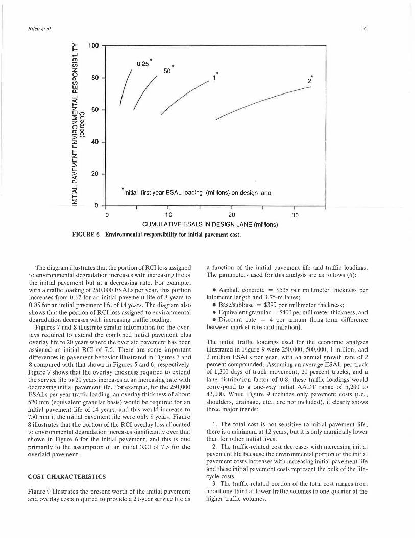
Figure 6 illustrates the portion of the RCI loss of an initial pavement that may be assigned to environmental degradation as a function of the cumulative ESAL loading and the life of the initial pavement. The function closest to the origin is for an initial ESAL loading of 250,000 per year, while the fourth function is for an initial ESAL loading of 2 million per year, both of which increase at 2 percent per year.

'E _§_

1000

(/) 800 (/) w z ~ g I I- 600 a: :) ::)

z <( a: CJ 1-z w _J <(

400

§5 200

a w

0

initial RCI = 8.5 RCI after overlay = 7.5 minimum RCI 5.5 ESAL growth rate = 2%

10 20

6 8 10 12 14 16

pavement life (years)

30

CUMULATIVE ESALS IN DESIGN LANE (millions)

FIGURE 5 Equivalent granular thickness versus design ESALs for different pavement lives.

Rilett et al.

~ 100 ::J ro en z 2 80 en w a: -' ~ z 60 w~

~c: z Q)

o~ !:!:; ~ >~

z 40 w 1-z w ~ w ~ 20

35

• 0.25

• 2

• a.. -' <( ;:::: initial first year ESAL loading (millions) on design lane

z 0

0 10 20 30

CUMULATIVE ESALS IN DESIGN LANE (millions)

FIGURE 6 Environmental responsibility for initial pavement cost.

The diagram illustrates that the portion of RCI loss assigned to environmental degradation increases with increasing life of the initial pavement but at a decreasing rate. For example, with a traffic loading of 250,000 ESALs per year, this portion increases from 0.62 for an initial pavement life of 8 years to 0.85 for an initial pavement life of 14 years. The diagram also shows that the portion of RCI loss assigned to environmental degradation decreases with increasing traffic loading.

Figures 7 and 8 illustrate similar information for the over­lays required to extend the combined initial pavement plus overlay life to 20 years where the overlaid pavement has been assigned an initial RCI of 7.5. There are some important differences in pavement behavior illustrated in Figures 7 and 8 compared with that shown in Figures 5 and 6, respectively. Figure 7 shows that the overlay thickness required to extend the service life to 20 years increases at an increasing rate with decreasing initial pavement life. For example, for the 250,000 ESALs per year traffic loading, an overlay thickness of about 520 mm (equivalent granular basis) would be required for an initial pavement life of 14 years, and this would increase to 750 mm if the initial pavement life were only 8 years. Figure 8 illustrates that the portion of the RCI overlay loss allocated to environmental degradation increases significantly over that shown in Figure 6 for the initial pavement, and this is due primarily to the assumption of an initial RCI of 7 .5 for the overlaid pavement.

COST CHARACTERISTICS

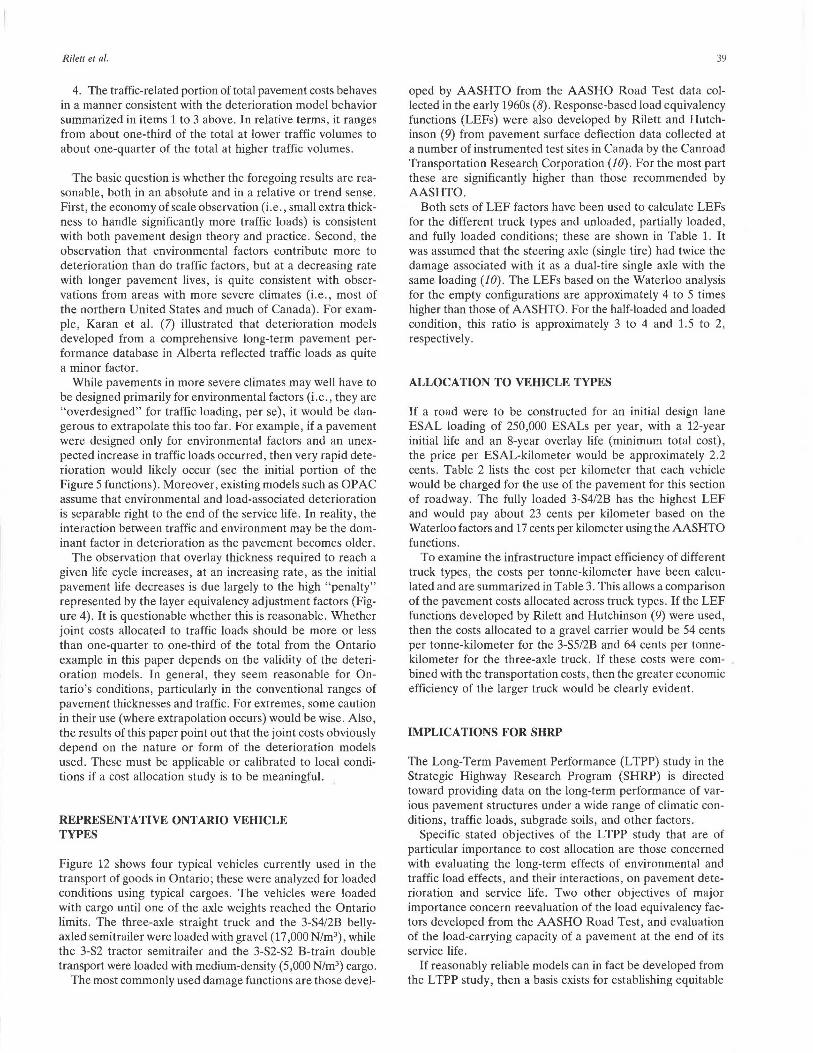
Figure 9 illustrates the present worth of the initial pavement and overlay costs required to provide a 20-year service life as

a function of the initial pavement life and traffic loadings. The parameters used for this analysis are as follows (6):

• Asphalt concrete = $538 per millimeter thickness per kilometer length and 3.75-m lanes;

• Base/subbase = $390 per millimeter thickness; • Equivalent granular = $400 per millimeter thickness; and • Discount rate = 4 per annum (long-term difference

between market rate and inflation).

The initial traffic loadings used for the economic analyses illustrated in Figure 9 were 250,000, 500,000, 1 million, and 2 million ESALs per year, with an annual growth rate of 2 percent compounded. Assuming an average ESAL per truck of 1,300 days of truck movement, 20 percent trucks, and a lane distribution factor of 0.8, these traffic loadings would correspond to a one-way initial AADT range of 5,200 to 42,000. While Figure 9 includes only pavement costs (i.e., shoulders, drainage, etc. , are not included), it clearly shows three major trends:

1. The total cost is not sensitive to initial pavement life; there is a minimum at 12 years, but it is only marginally lower than for other initial lives.

2. The traffic-related cost decreases with increasing initial pavement life because the environmental portion of the initial pavement costs increases with increasing initial pavement life and these initial pavement costs represent the bulk of the life­cycle costs.

3. The traffic-related portion of the total cost ranges from about one-third at lower traffic volumes to one-quarter at the higher traffic volumes.

E 1000

.s en en w z 800 ~ (_)

:I I-a: :s 600 :::> z c( a: Cl I-z 400 w ...J

~ :::> a w 200 >-:s a: w > 0 0

FIGURE 7

~ ::J iii en ao z 0 Cl. en w a: <l. ~ 60 I- c: z Q)

w~ :: Q)

z ..e: 0 a: 5 z w

~ a: w > 0

40

20

!!·/ ,.--• 0.25

• initial first year ESAL loading (millions) on design lane

0 10 20 30 CUMULATIVE ESALS IN DESIGN LANE (millions)

Equivalent granular thickness of overlays for different traffic load intensities.

• 0.25 • . 50 • 1 •

2

• initial first year ESAL loading (millions) on design lane

0 10 20 30 CUMULATIVE ESALS IN DESIGN LANE (millions)

FIGURE 8 Environmental responsibility for overlay cost.

Rileu et al. 37

* initial first year ESAL loading (millions) on design lane

800 en tn o_ o E ~! 600 I c: I-~ a: (\I 0'-~ ~ I- _Ill 400 zo WO cno w .-a:~ a...-

200

6

* design ESAL's 2.0 1.0 0.5 0.25

* design ESAL's 2.0 1.0 0.5

0.25

8 10 12 14

total costs

costs allocated to traffic

16

INITIAL PAVEMENT LIFE (years) FIGURE 9 Present worth of initial pavement plus overlay costs.

These trends are all consistent with observations from the deterioration-related graphs (Figures 5 to 8). It might also be noted in Figure 9 that the increase of either total cost or traffic­related cost, for any initial pavement life, increases approx­imately uniformly for each doubling of traffic loads. In effect, this becomes a surrogate for pavement thickness and, similar to Figure 5, illustrates the economies of scale that exist for pavements with respect to traffic loading.

The joint com in dollars per ESAL-kilometer were cal­culated by dividing the present worths of the traffic-related life-cycle costs by the present worths of the ESAL versus time profile specified for the design. This approach was taken as it was argued that the consumption of pavement RCI by vehi­cles has a time base similar to that of pavement costs. This approach is particularly important for situations in which annual traffic loads are increasing.

Figure 10 illustrates the joint costs in dollars per ESAL­kilometer as a function of the cumulative ESALs and the initial pavement life, for the same conditions as in Figure 9. For example, at the lower traffic volume, 250,000 ESALs per year initially, the joint cost would be about 2.6 cents per ESAL-kilometer for an initial pavement life of 10 years. This would drop to about 0.6 cents per ESAL-kilometer for the higher volume of 2 x 106 ESALs per year initially and an initial pavement life of 10 years. While the cost per ESAL­kilometer drops significantly with increasing traffic, the total cost of the pavement would , of course, be higher. Again, it illustrates the economies of scale for thicker pavements and higher traffic volumes. The degree to which these joint costs are actually being met by taxation revenues was not a part of this study.

Figure 11 shows the joint costs as a function of cumulative ESALs for a minor highway (i.e. , minimum RCI of 4.5 and

initial traffic loadings of 75,000, 150,000, and 300,000 ESALs per year, increasing at 2 percent per year). In this case the joint costs, particularly at the lower rates, are substantially higher than those shown in Figure 10, as might be expected .

ENVIRONMENTAL VERSUS TRAFFIC ALLOCATION OF DETERIORATION

The foregoing sections show that if a deterioration model exists with the capability of separating the contributions of traffic and environment, then the life-cycle costs attributable to traffic can be calculated. In the Ontario method ESALs are the variable used to predict load-associated deterioration and may therefore be used as the responsibility measure for joint costs .

For the particular deterioration model used in the sample allocation, the following major points emerge:

1. The absolute required pavement thickness always increases with increasing cumulative ESALs, but the rate of change decreases. This illustrates an economy of scale in that a small extra thickness can carry substantially more traffic loads.

2. The portion of deterioration due to environmental fac­tors is generally greater than that due to traffic loads. More­over, this portion increases with increasing life of the pave­ment but at a decreasing rate .

3. For a fixed life cycle (say, 20 years) the overlay thickness required increases at an increasing rate, as the initial pave­ment service life becomes shorter. This means that the portion of the deterioration of the resurfaced pavement due to envi­ronmental factors increases significantly compared with the initial pavement.

4

3 initial pavement life (years)

8 10 12 14

2

0 10 20 30 40 50 CUMULATIVE ESALS (millions)

FIGURE 10 Joint costs for a primary highway.

8

7

initial pavement life (years) 8 10 i2 14

0

0 2 4 6 8 10

CUMULATIVE ESALS (millions)

FIGURE 11 Joint costs for a secondary highway.

Rilett et al.

4. The traffic-related portion of total pavement costs behaves in a manner consistent with the deterioration model behavior summarized in items 1 to 3 above. In relative terms, it ranges from about one-third of the total at lower traffic volumes to about one-quarter of the total at higher traffic volumes.

The basic question is whether the foregoing results are rea­sonable, both in an absolute and in a relative or trend sense. First, the economy of scale observation (i.e., small extra thick­ness to handle significantly more traffic loads) is consistent with both pavement design theory and practice. Second, the observation that environmental factors contribute more to deterioration than do traffic factors, but at a decreasing rate with longer pavement lives, is quite consistent with obser­vations from areas with more severe climates (i.e., most of the northern United States and much of Canada). For exam­ple, Karan et al. (7) illustrated that deterioration models developed from a comprehensive long-term pavement per­formance database in Alberta reflected traffic loads as quite a minor factor.

While pavements in more severe climates may well have to be designed primarily for environmental factors (i.e., they are "overdesigned" for traffic loading, per se), it would be dan­gerous to extrapolate this too far. For example, if a pavement were designed only for environmental factors and an unex­pected increase in traffic loads occurred, then very rapid dete­rioration would likely occur (see the initial portion of the Figure 5 functions). Moreover, existing models such as OP AC assume that environmental and load-associated deterioration is separable right to the end of the service life. In reality, the interaction between traffic and environment may be the dom­inant factor in deterioration as the pavement becomes older.

The observation that overlay thickness required to reach a given life cycle increases, at an increasing rate, as the initial pavement life decreases is due largely to the high "penalty" represented by the layer equivalency adjustment factors (Fig­ure 4) . It is questionable whether this is reasonable. Whether joint costs allocated to traffic loads should be more or less than one-quarter to one-third of the total from the Ontario example in this paper depends on the validity of the deteri­oration models . In general , they seem reasonable for On­tario's conditions, particularly in the conventional ranges of pavement thicknesses and traffic. For extremes, some caution in their use (where extrapolation occurs) would be wise . Also, the results of this paper point out that the joint costs obviously depend on the nature or form of the deterioration models used. These must be applicable or calibrated to local condi­tions if a cost allocation study is to be meaningful.

REPRESENTATIVE ONTARIO VEHICLE TYPES

Figure 12 shows four typical vehicles currently used in the transport of goods in Ontario; these were analyzed for loaded conditions using typical cargoes. The vehicles were loaded with cargo until one of the axle weights reached the Ontario limits . The three-axle straight truck and the 3-S4/2B belly­axled semitrailer were loaded. with gravel (17 ,000 N/m3), while the 3-S2 tractor semitrailer and the 3-S2-S2 B-train double transport were loaded with medium-density (5,000 N/m3) cargo.

The most commonly used damage functions are those <level-

39

oped by AASHTO from the AASHO Road Test data col­lected in the early 1960s (8). Response-based load equivalency functions (LEFs) were also developed by Rilett and Hutch­inson (9) from pavement surface deflection data collected at a number of instrumented test sites in Canada by the Canroad Transportation Research Corporation (10); For the most part these are significantly higher than those recommended by AASHTO.

Both sets of LEF factors have been used to calculate LEFs for the different truck types and unloaded, partially loaded, and fully loaded conditions; these are shown in Table 1. It was assumed that the steering axle (single tire) had twice the damage associated with it as a dual-tire single axle with the same loading (JO). The LEFs based on the Waterloo analysis for the empty configurations are approximately 4 to 5 times higher than those of AASHTO. For the half-loaded and loaded condition, this ratio is approximately 3 to 4 and 1.5 to 2, respectively.

ALLOCATION TO VEHICLE TYPES

If a road were to be constructed for an initial design lane ESAL loading of 250,000 ESALs per year, with a 12-year initial life and an 8-year overlay life (minimu~ total cost), the price per ESAL-kilometer would be approximately 2.2 cents. Table 2 lists the cost per kilometer that each vehicle would be charged for the use of the pavement for this section of roadway. The fully loaded 3-S4/2B has the highest LEF and would pay about 23 cents per kilometer based on the Waterloo factors and 17 cents per kilometer using the AASHTO functions.

To examine the infrastructure impact efficiency of different truck types, the costs per tonne-kilometer have been calcu­lated and are summarized in Table 3. This allows a comparison of the pavement costs allocated across truck types. If the LEF functions developed by Rilett and Hutchinson (9) were used, then the costs allocated to a gravel carrier would be 54 cents per tonne-kilometer for the 3-S5/2B and 64 cents per tonne­kilometer for the three-axle truck. If these costs were com­bined with the transportation costs, then the greater economic efficiency of the larger truck would be clearly evident.

IMPLICATIONS FOR SHRP

The Long-Term Pavement Performance (LTPP) study in the Strategic Highway Research Program (SHRP) is directed toward providing data on the long-term performance of var­ious pavement structures under a wide range of climatic con­ditions, traffic loads, subgrade soils, and other factors.

Specific stated objectives of the LTPP study that are of particular importance to cost allocation are those concerned with evaluating the long-term effects of environmental and traffic load effects, and their interactions, on pavement dete­rioration and service life. Two other objectives of major importance concern reevaluation of the load equivalency fac­tors developed from the AASHO Road Test, and evaluation of the load-carrying capacity of a pavement at the end of its service life.

If reasonably reliable models can in fact be developed from the L TPP study, then a basis exists for establishing equitable

40 TRANSPORTATION RESEARCH RECORD 1215

3-Axle Straight Truck

3-52 tractor semi-trailer

3-55/28 tractor semi-trailer

tare = 8 61 9 kg Payload:

tare = 8 200 kg tare = 6 300 kg Payload:

tare = 8 200 kg tare = 8 300 kg Payload:

cargo density = 17 000 N/m3 8 034 kg (half full)

cargo density = 1 000 N/m3 12 360 kg (half full)

14 .63 m

10.59m

cargo density = 17 000 N/m3 21 120 kg (half full)

GVM = 24 686 kg 16 068 kg (full)

GVM = 39 220 kg 24 720 kg (full)

GVM = 58 740 kg 42 240 kg (full)

a11 1111 1 1~111 1~111 1 111 3-52-52 tractor 1st semi-trailer 2nd semi-trailer

I+- 4.82m -+!+- 4.59m -+l+-3 .00m-+l+-4.15m-+I

cargo density = 17 000 N/m3 GVM = 45 836 kg

tare = 8 200 kg tare = 6 000 kg tare = 4 300 kg Payload: 13 433 kg (half full) 26 866 kg (full)

l+4.82m ... •l4---12.17m --~•"414--6 .25m~

FIGURE 12 Representative Ontario trucks.

cost allocation polici s. This would include an abi lity to cap­ture the increasing effect of traffic load on pavement dete­rioration (i.e. , through modeling the interaction between environment and traffic) as the pavement age . The premise is that traffic has a more severe effect on older pavement both through this interaction and because of the increase in dynamic load effects (11).

real benefit (i .e., cost saving) in paying for better roads as opposed to paying only for their rehabilitation in advanced states of deterioration. This would be in addition to the sub­stantial agency savings on investment costs plus vehicle oper­ating cost savings realized by early rehabilitation (12) .

Because only a limited number of pavement deterioration models exist that separately identify traffic load- and envi­ronment-associated contributions, and because these are gen-The implication for cost allocation is that there could be a

Ritell el al.

TABLE 1 LOAD EQUIVALENCY FUNCTIONS FOR REPRESENTATIVE TRUCKS

TRUCK Loading TYPE Empty Half Full

3 AXLE 0.54 1.88 4.66 (0. 07) (0,62) (3.03)

3-S2 0.99 2.60 6.34 (0.20) (0.80) (3.74)

3-S4/2B 1.12 3.67 10.40 (0 . 23) (1.21) (7. 80)

3-S2-S2 1. 03 2 . 45 5.40 (0 . 25) (0.62) (2.54)

the upper entries in each cell are LEFs calculated from LEF functions reported by Rilett & Hutchinson and those in parentheses are calulated from the AASHTO functions

TABLE 2 JOINT PAVEMENT COSTS PER VEHICLE-KILOMETER

TRUCK Loading

TYPE Empty Half Full

3 AXLE 1.19 4.14 10.25 (0.15) ( 1. 36) (6.67)

3-S2 2.18 5 . 72 13. 95 (0.44) (1.76) (8.23)

3-S4/2B 2.46 8 . 07 22.88 (0.51) (2.66) (17 . 16)

3-S2-S2 2 . 27 5 . 39 ll. 88 (0 . 55) (1.36) (5.59)

entries are cents per kilometer; the upper entries are calcuiated from LEF functions reported by Rilett and Hutchinson and the lower entries are the costs calculated from the AASHTO LEF functions

TABLE 3 JOINT PAVEMENT COSTS PER TONNE­KILOMETER

TRUCK Loading

TYPE Half Full

3 AXLE 0.51 0.64 (0 .17) (0.41)

3-S2 0 . 46 0.56 (0.14) (0.33)

3-S4/2B 0.38 0.54 (0.13) (0.41)

3-S2-S2 0 . 40 0.44 (0 . 10) (0.21)

entries are cents per kilometer; the upper entries are calculated from LEF functions reported by Rilett and Hutchinson and the lower entries are the costs calculated from the AASHTO LEF functions

41

erally limited to a regional set of conditions, the models even­tually developed from the L TPP study in SHRP should be able finally to establish the comprehensive technical basis needed for equitable cost allocation.

CONCLUDING REMARKS

Flexible pavement deterioration models that incorporate both load-associated and environment-associated deterioration components allow long-term pavement life-cycle costs to be split into joint and common costs. Joint pavement costs may then be allocated to vehicle classes using an ESAL-kilometer responsibility measure, and common costs may be allocated in proportion to the number of vehicles in each class.

The Ontario flexible pavement deterioration model exhibits the characteristics typical of many deterioration models. There are economies of scale in pavement thickness with respect to increasing traffic loads for a given initial pavement life. How­ever, pavement thickness increases at an increasing rate with increases in the initial pavement life.

Use of the Ontario pavement deterioration model for cost allocation for a representative primary highway pavement sec­tion suggested that the portion of pavement costs allocated to environmental degradation and, therefore, to common costs varies between 55 and 88 percent, depending on the intensity of the traffic loading and the length of the initial pavement life chosen. For example, for a pavement experiencing 250,000 ESALs per year, the portion allocated to environmental deg­radation increases from about 62 percent for an initial design life of 8 years to 84 percent for a design life of 16 years. With a pavement experiencing 2 million ESALs per year, the por­tion allocated to environmental degradation increases from 55 percent for a design life of 8 years to 72 percent for a design life of 16 years.

Analysis of the performance of overlays showed similar trends but with higher portions of the overlay costs being allocated to environmental degradation. These higher allo­cations to environmental degradation reflect the larger reduc­tions in strength of the original pavement layers assigned by the Ontario method and the use of an initial RCI of 7.5 for the overlaid pavement.

Analysis of the total life-cycle pavement costs for given traffic loadings showed that they were relatively insensitive to the initial design life selected, with a fairly weak minimum occurring at about 12 years. The joint cost allocated to traffic varied from about 1.8 cents per ESAL-kilometer at a traffic loading of 250,000 ESALs per year to 0.5 cent per ESAL­kilometer for a traffic loading of 2 million ESALs per year.

Analysis of representative Ontario vehicle types showed that the fully loaded tonne-kilometer joint cost varied from 0.64 cents per tonne-kilometer for a three-axle gravel truck to 0.44 cents per tonne-kilometer for a B-train double trans­porting medium-density cargo.

The results of the cost allocation calculations presented in this paper are critically dependent upon the structure and integrity of the pavement deterioration model used. While the Ontario method seems to capture the performance of initial pavements, there is some question about the perfor­mance prediction of pavements with overlays. This is a critical issue in many jurisdictions, because the systems are mature

42

and most of the pavement work involves rehabilitation and resurfacing.

ACKNOWLEDGMENTS

The work on which this paper is based was funded by the Natural Sciences and Engineering Research Council of Canada, and this support is gratefully acknowledged.

REFERENCES

1. T. F. Wong and M. J. Markow. Allocation of Life-Cycle Highway Pavement Costs. Report FHWA/RD-83/030. FHWA, U.S. Department of Transportation, 1984.

2. N. Kamel. Developing Structural Design Models for Ontario Pavements. In Transportation Research Record 521, TRB, National Research Council, Washington, D.C., 1974, pp. 60-72.

3. F. W. Jung, R. Kher, and W. A. Phang. A Performance Pre­diction Subsystem-Flexible Pavement. RR 200. Ontario Ministry of Transportation and Communications, Toronto, Ontario, Can­ada, 1975.

4. J . B. Rauhut, R. L. Lytton, and M. I. Darter. Pavement Damage Functions for Cost Allocation. Report FHW A/RD-84/108. FHWA, U.S. Department of Transportation, June 1984.

5. R. Haas, M. Van Aerde, and R. Penner. Vehicle Operating Costs and Pavement Damage Functions for Highway Cost Allocation. Prepared for the CTRF-RTAC Workshop on Highway Finance, Toronto, Ontario, Canada, 1985.

TRANSPORTATION RESEARCH RECORD 1215

6. R. Haas and T. Papagiannakis . Impacts of Heavy Vehicles on Urban Pavements. Paper prepared for the Annual Conference of the Roads and Transportation Association of Canada, Saskatoon, Saskatchewan, Canada, 1987.

7. M.A. Karan, T. J. Christison, A. Cheetham, and G. Berdahl. Development and Implementation of Alberta's Pavement Infor­mation and Needs System (PINS). In Transportation Research Record 938, TRB, National Research Council, Washington, D.C., 1983, pp. 11-20.

8. AASHTO Guide for the De,fign of Fl~xihlf PnVl'm fnts . American Association of State Highway and Transportation Officials, Washington, D.C. , 1986.

9. L. R. Rilett, and B. G. Hutchinson . LEF Functions from Can­road Pavement Load-Deflection Data. In Transportation Research Record 1196, TRB, National Research Council, Washington, D. C., 1988, pp. 170-178.

10. J. T. Christison. Pavement Response to Heavy Vehicle Test Pro­gram: Part I-Data Summary Report. Canroad Transportation Research Corporation, Ottawa, Ontario, Canada, 1986.

11. A. T. Papagiannakis, R. C. G. Haas, J. H.F. Woodroofe, and P. A. LeBlanc. Impact of Roughness-Induced Dynamic Loads on Flexible Pavement Distress and Performance. Proc., First International Symposium on Surface Characteristics, State Col­lege, Pa., June 1988.

12. R. Haas. The Long Term Effects of Spending Decisions on Paved Roads. Proc., Eurasphalt Congress, Berlin, West Germany, May 1984.

Publication of this paper sponsored by Committee on Pavement Management Systems.