Cosmology from

Secondary Anisotropies

of the

Cosmic Microwave Background

Blake Daniel Sherwin

A Dissertation

Presented to the Faculty

of Princeton University

in Candidacy for the Degree

of Doctor of Philosophy

Recommended for Acceptance

by the Department of

Physics

Adviser: Prof. David N. Spergel

September 2013

c© Copyright by Blake Daniel Sherwin, 2013.

All rights reserved.

Abstract

Gravitational lensing and the Sunyaev-Zel’dovich effect introduce new intensity fluc-

tuations, known as secondary anisotropies, into the cosmic microwave background

radiation (CMB). These CMB secondary anisotropies encode a wealth of information

about the distribution of dark matter and gas throughout our universe. In this thesis,

we present novel measurements of CMB lensing and the Sunyaev-Zel’dovich effect in

the microwave background and use them to place new constraints on cosmology.

In an early thesis chapter, we describe the first detection of the power spectrum

of gravitational lensing of the CMB. The power spectrum is detected at a four sigma

significance through a measurement of the four-point correlation function of Atacama

Cosmology Telescope (ACT) CMB temperature maps. This first detection gravita-

tionally probes the amplitude of large-scale structure at redshifts ≈ 1 − 3 to 12%

accuracy, and lies at the beginning of an exciting new field of science with the lensing

power spectrum.

From this measurement of the CMB lensing power spectrum we extract first cos-

mological constraints. We explain in detail how the amount of dark energy in our

universe affects the amplitude of the lensing signal by modifying both the geometry

of the universe and the growth of structure. We then demonstrate that our lensing

measurements provide, for the first time, evidence for the existence of dark energy

from the CMB alone, at a 3.2 sigma significance.

We use CMB lensing measurements to study the relation of quasars to the under-

lying distribution of dark matter. Detecting the cross-power of CMB lensing with the

spatial distribution of quasars and hence measuring the quasar bias to within 25%,

we obtain a measurement of the characteristic dark matter halo mass of these objects.

CMB lensing power spectrum measurements typically require the subtraction of

a simulated bias term, which complicates the analysis; we develop new techniques to

obviate this bias subtraction.

iii

Finally, we develop a novel method for measuring the Sunyaev-Zel’dovich effect

through the skewness it induces in CMB temperature maps. Detecting this skewness

in ACT CMB maps for the first time at five sigma significance, we demonstrate how

this novel measurement constrains the amplitude of structure in our universe to within

4%.

iv

Acknowledgements

First and foremost, I would like to thank my adviser David Spergel, as I owe nearly

all my scientific achievements to his guidance and teaching. It has been a joy and a

great privilege to work with him over the last few years.

I have been fortunate to collaborate with truly outstanding scientists. In particu-

lar, Sudeep Das has served as a second advisor for me in our continuing collaboration

on CMB lensing and has also been responsible for much of my success. I am grateful

to Matias Zaldarriaga for an interesting collaboration, for much helpful advice, and

for agreeing to be a reader for my thesis. I thank Lyman Page, Jo Dunkley and

everyone working on ACT for interesting and successful research collaborations as

well as general advice. I thank Suzanne Staggs for collaboration and for advising my

experimental project. I am also grateful to Bill Jones and Igor Klebanov for agreeing

to serve on my thesis committee.

Before coming to Princeton, my interest in physics and cosmology was encouraged

by a number of excellent teachers and scientists, such as Elizabeth Parr, Helmut

Kuehnberger, Mike Hobson, John Kirk, Donald Lynden-Bell and Avi Loeb, and I

thank them for their teaching and inspiration.

I am grateful to my friends for making graduate school enjoyable even when work

was stressful. I would like to thank David McGady for his friendship and for his

ability to tolerate me as an apartment-mate – not always an easy task – and am

similarly grateful to Guilherme Pimentel, Halil Saka and Colin Hill (who also belongs

in the outstanding collaborators paragraph). I would also like to thank Katrina Jones,

Anushya Chandran, Michael Mooney, Eduardo da Silva Neto, Leah Klement, Eaming

Wu and Matt Johnson for friendship and some great times.

I thank Maryam Patton for her love and encouragement, which have made the

last few years some of the best of my life. Any success I have had in graduate school

would not have been possible without her support.

v

Finally, I would like to thank my family. I am truly fortunate to have parents

and a sister who have always encouraged me in my academic pursuits, no matter how

obscure they may have seemed to them, and have always believed in me as a scientist

and as a person. Without their support in difficult times and the knowledge that I

always have a loving family to fall back on, I wouldn’t have achieved much at all, let

alone written a Ph.D. thesis in Physics.

vi

In memory of my friend Arunn Mahakuperan

vii

Relation to Published Work

This thesis consists of seven chapters. The first two chapters are introductory and

summarize relevant past research on CMB secondary anisotropies; in these chapters,

I thus claim originality only in the details of exposition.

The central part of this thesis is formed by chapters three through seven. These

chapters have, in slightly modified form, either been published in or submitted to

peer reviewed journals. I will here note the publication or submission status of each

chapter. As all the projects listed here were completed as part of a research col-

laboration, I will also attempt to describe my own contribution to each of the chapters.

Chapter 3: Detection of the Power Spectrum of CMB Lensing with the

Atacama Cosmology Telescope

Das, S., Sherwin, B. D., et al. 2011, Physical Review Letters., 112, 021301; the

appendix is from Das, S. et al. 2013, arXiv:1301.1037, Journal of Cosmology and

Astroparticle Physics submitted

The work described in this chapter was performed mainly by Sudeep Das and

myself under the guidance of David Spergel, though it relied crucially on data taken

by the Atacama Cosmology Telescope collaboration (of which I am a part). I wrote

most of the core computational pipeline that performs the lensing reconstruction

from high-resolution temperature maps under the guidance of Sudeep Das. I also

developed and ran many of the required null and systematic tests in this paper.

viii

Sudeep Das and I made equal contributions to the development of codes to calculate

errors and biases and to compile the final results. The text was written by myself,

David Spergel and Sudeep Das. The updated lensing power spectrum calculation

from the new dataset and the text in the addendum to the chapter is my work,

though it relies on older jointly-developed codes.

Chapter 4: Evidence for Dark Energy from the CMB Alone Using ACT

Lensing Measurements

Sherwin, B. D., Dunkley, J., Das, S., et al. 2011, Physical Review Letters, 112, 021302

The work described in this chapter was performed mainly by myself, Joanna

Dunkley and Sudeep Das, relying again on data from the Atacama Cosmology

Telescope collaboration. I developed and tested the final form for the likelihood with

Joanna Dunkley, processed and analyzed the chains, and calculated the cosmological

constraints described in this paper. I also developed and tested the physical explana-

tions of how lensing constrains dark energy, and wrote the text of the chapter. The

lensing measurements underlying these results, made by Sudeep Das, myself, and

others, are described in Chapter 2.

Chapter 5: Cross-correlation of CMB Lensing with the Distribution of

Quasars

Sherwin, B. D., Das, S., Hajian, A. et al. 2012, Physical Review D, 86, 083006

Nearly all the results and text described in this section are my own work, under

the guidance of David Spergel, though the lensing measurement again relies on

data from the Atacama Cosmology Telescope, Amir Hajian constructed the quasar

maps from the SDSS catalog, and Sudeep Das contributed tests of my theory curve

calculation.

ix

Chapter 6: CMB Lensing: Power Without Bias

Sherwin, B. D., & Das, S. 2010, arXiv:1011.4510

The idea for this chapter arose from conversations with Sudeep Das. I worked out

the details of the no-bias method presented here, including the expansion formalism,

with input from Sudeep Das and guidance from David Spergel. The testing of the

method on simulations was joint work with Sudeep Das.

Chapter 7: A Measurement of the Skewness of the Thermal Sunyaev-

Zeldovich Effect

Wilson, M. J., Sherwin, B. D., et al. 2012, Physical Review D, 86, 122005

This final chapter was a joint effort between Michael Wilson (an undergraduate

whom I advised), myself, and Colin Hill. I developed the idea for this project and

supervised Michael Wilson’s work in great detail. I wrote my own codes and verified

all the results Michael Wilson obtained prior to publication. I also generated the

required simulations of the observed full CMB sky, relying on Sunyaev-Zel’dovich

simulations by Nick Battaglia. I wrote most of the text for this chapter/publication,

with contributions and editing from Colin Hill.

Appendix A: Lensing Simulation and Power Spectrum Estimation for High

Resolution CMB Polarization Maps

Louis, T., Naess, S., Das, S., Dunkley, J., Sherwin, B., 2013, arXiv:1306.6692

This project was lead by Thibaut Louis and Sigurd Naess (and is hence relegated

to an appendix), though I contributed to the paper: Thibaut and I independently

performed all the derivations of the expressions in section A.3, and I helped develop

the new method for simulating polarized lensing rapidly. In addition, the code which

inverts the mode-coupling matrix is based on my work on the ACT temperature power

spectrum pipeline.

x

Contents

Abstract . . . . . . . . . . . . . . . . . . . . . . . . . . . . . . . . . . . . . iii

Acknowledgements . . . . . . . . . . . . . . . . . . . . . . . . . . . . . . . v

Relation to Published Work . . . . . . . . . . . . . . . . . . . . . . . . . . viii

List of Tables . . . . . . . . . . . . . . . . . . . . . . . . . . . . . . . . . . xv

List of Figures . . . . . . . . . . . . . . . . . . . . . . . . . . . . . . . . . . xvi

1 Introduction 1

1.1 CMB Secondary Anisotropies as a New Source of Cosmological Infor-

mation . . . . . . . . . . . . . . . . . . . . . . . . . . . . . . . . . . . 1

1.2 Overview of this Thesis . . . . . . . . . . . . . . . . . . . . . . . . . . 5

2 Brief Review of CMB Lensing Reconstruction Theory 8

2.1 Lensing of the CMB . . . . . . . . . . . . . . . . . . . . . . . . . . . 8

2.2 Lensing Reconstruction . . . . . . . . . . . . . . . . . . . . . . . . . . 11

3 Detection of the Power Spectrum of CMB Lensing with the Atacama

Cosmology Telescope 17

3.1 Abstract . . . . . . . . . . . . . . . . . . . . . . . . . . . . . . . . . . 17

3.2 Introduction . . . . . . . . . . . . . . . . . . . . . . . . . . . . . . . . 18

3.3 Data . . . . . . . . . . . . . . . . . . . . . . . . . . . . . . . . . . . . 18

3.4 Methods . . . . . . . . . . . . . . . . . . . . . . . . . . . . . . . . . . 19

3.5 Simulations . . . . . . . . . . . . . . . . . . . . . . . . . . . . . . . . 21

xi

3.6 Results . . . . . . . . . . . . . . . . . . . . . . . . . . . . . . . . . . . 22

3.7 Null Tests . . . . . . . . . . . . . . . . . . . . . . . . . . . . . . . . . 25

3.8 Implications and Conclusions . . . . . . . . . . . . . . . . . . . . . . 26

3.9 Acknowledgements . . . . . . . . . . . . . . . . . . . . . . . . . . . . 26

3.10 Addendum: Updated Measurement of the Lensing Power Spectrum

from Three Seasons of Data . . . . . . . . . . . . . . . . . . . . . . . 27

4 Evidence for Dark Energy from the CMB Alone Using ACT Lensing

Measurements 33

4.1 Abstract . . . . . . . . . . . . . . . . . . . . . . . . . . . . . . . . . . 33

4.2 Introduction . . . . . . . . . . . . . . . . . . . . . . . . . . . . . . . . 34

4.3 Methodology . . . . . . . . . . . . . . . . . . . . . . . . . . . . . . . 39

4.4 Results . . . . . . . . . . . . . . . . . . . . . . . . . . . . . . . . . . . 40

4.5 Conclusions . . . . . . . . . . . . . . . . . . . . . . . . . . . . . . . . 41

4.6 Acknowledgements . . . . . . . . . . . . . . . . . . . . . . . . . . . . 42

5 Cross-correlation of CMB Lensing with the Distribution of Quasars 46

5.1 Abstract . . . . . . . . . . . . . . . . . . . . . . . . . . . . . . . . . . 46

5.2 Introduction . . . . . . . . . . . . . . . . . . . . . . . . . . . . . . . . 47

5.3 Theoretical Background . . . . . . . . . . . . . . . . . . . . . . . . . 48

5.4 Cross-correlating CMB Lensing and Quasars . . . . . . . . . . . . . . 50

5.4.1 The ACT CMB Lensing Convergence Maps . . . . . . . . . . 50

5.4.2 The SDSS Quasar Maps . . . . . . . . . . . . . . . . . . . . . 52

5.4.3 The CMB Lensing - Quasar Cross-Power Spectrum . . . . . . 53

5.5 A Constraint on the Quasar Bias . . . . . . . . . . . . . . . . . . . . 56

5.6 Testing the power spectrum . . . . . . . . . . . . . . . . . . . . . . . 58

5.6.1 Null Tests . . . . . . . . . . . . . . . . . . . . . . . . . . . . . 58

5.6.2 Estimating Potential Systematic Contamination . . . . . . . . 58

xii

5.7 Summary and Conclusions . . . . . . . . . . . . . . . . . . . . . . . . 61

5.8 Acknowledgements . . . . . . . . . . . . . . . . . . . . . . . . . . . . 62

6 CMB Lensing: Power Without Bias 67

6.1 Abstract . . . . . . . . . . . . . . . . . . . . . . . . . . . . . . . . . . 67

6.2 Bias-free Lensing Power Spectrum Measurements . . . . . . . . . . . 68

6.3 Acknowledgements . . . . . . . . . . . . . . . . . . . . . . . . . . . . 76

7 A Measurement of the Skewness of the Thermal Sunyaev-Zeldovich

Effect 79

7.1 Abstract . . . . . . . . . . . . . . . . . . . . . . . . . . . . . . . . . . 79

7.2 Introduction . . . . . . . . . . . . . . . . . . . . . . . . . . . . . . . . 80

7.3 Skewness of the tSZ Effect . . . . . . . . . . . . . . . . . . . . . . . . 83

7.4 Map Processing . . . . . . . . . . . . . . . . . . . . . . . . . . . . . . 87

7.4.1 Filtering the Maps . . . . . . . . . . . . . . . . . . . . . . . . 87

7.4.2 Removing Point Sources . . . . . . . . . . . . . . . . . . . . . 88

7.5 Results . . . . . . . . . . . . . . . . . . . . . . . . . . . . . . . . . . . 90

7.5.1 Evaluating the Skewness . . . . . . . . . . . . . . . . . . . . . 90

7.5.2 The Origin of the Signal . . . . . . . . . . . . . . . . . . . . . 92

7.5.3 Testing for Systematic Infrared Source Contamination . . . . . 95

7.6 Cosmological Interpretation . . . . . . . . . . . . . . . . . . . . . . . 97

7.7 Conclusions . . . . . . . . . . . . . . . . . . . . . . . . . . . . . . . . 101

7.8 Acknowledgements . . . . . . . . . . . . . . . . . . . . . . . . . . . . 101

A Lensing Simulation and Power Spectrum Estimation for High Res-

olution CMB Polarization Maps 106

A.1 Abstract . . . . . . . . . . . . . . . . . . . . . . . . . . . . . . . . . . 106

A.2 Introduction . . . . . . . . . . . . . . . . . . . . . . . . . . . . . . . . 107

A.3 E/B leakage in the flat sky approximation . . . . . . . . . . . . . . . 108

xiii

A.3.1 Notation . . . . . . . . . . . . . . . . . . . . . . . . . . . . . . 108

A.3.2 Partial sky coverage . . . . . . . . . . . . . . . . . . . . . . . 110

A.3.3 Pure estimators . . . . . . . . . . . . . . . . . . . . . . . . . . 111

A.4 Generating gravitationally lensed simulations . . . . . . . . . . . . . . 113

A.5 Implementation on realistic observations . . . . . . . . . . . . . . . . 117

A.5.1 Estimated power spectra . . . . . . . . . . . . . . . . . . . . . 118

A.5.2 Power spectrum uncertainties . . . . . . . . . . . . . . . . . . 120

A.6 Conclusions . . . . . . . . . . . . . . . . . . . . . . . . . . . . . . . . 121

A.7 Acknowledgements . . . . . . . . . . . . . . . . . . . . . . . . . . . . 123

A.8 Error Calculation . . . . . . . . . . . . . . . . . . . . . . . . . . . . . 123

B Methods for CMB Lensing Estimation without Sensitivity to Fore-

grounds 127

B.1 Lensing Biases from Foregrounds . . . . . . . . . . . . . . . . . . . . 127

B.2 Immunizing the Lensing Estimator to Foreground Contamination . . 128

B.2.1 Poisson Foregrounds . . . . . . . . . . . . . . . . . . . . . . . 128

B.2.2 General Foregrounds . . . . . . . . . . . . . . . . . . . . . . . 131

xiv

List of Tables

3.1 Reconstructed Cκκ` values. . . . . . . . . . . . . . . . . . . . . . . . . 24

7.1 Constraints on σ8 derived from our skewness measurement using two

different simulations and three different scalings of the skewness and

its variance with σ8. The top row lists the simulations used to calculate

the expected skewness for σ8 = 0.8 [35, 33]; the left column lists the

pressure profiles used to calculate the scaling of the skewness and its

variance with σ8 [16, 17, 25]. The errors on σ8 shown are the 68% and

95% confidence levels. . . . . . . . . . . . . . . . . . . . . . . . . . . 100

xv

List of Figures

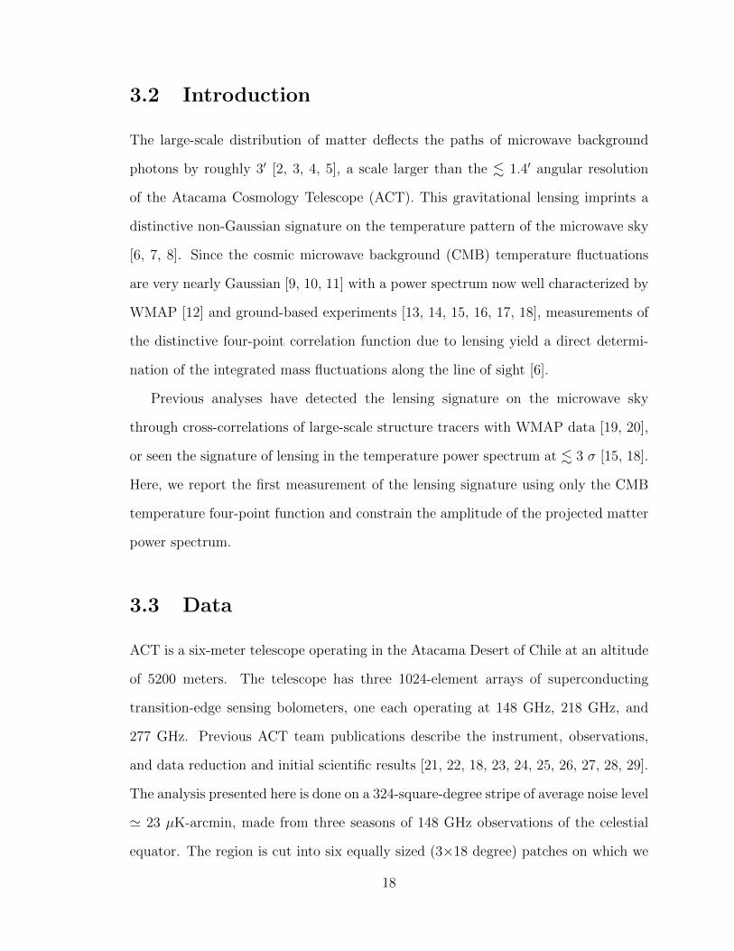
3.1 Mean convergence power spectrum (red points) from 480 simulated

lensed maps with noise similar to our data. The solid line is the input

lensing power spectrum, taken from the best-fit WMAP+ACT cosmo-

logical model. Error bars correspond to the scatter of power spectrum

values obtained from individual maps. . . . . . . . . . . . . . . . . . 22

3.2 Convergence power spectrum (red points) measured from ACT equa-

torial sky patches. The solid line is the power spectrum from the

best-fit WMAP+ACT cosmological model with amplitude AL = 1,

which is consistent with the measured points. The error bars are from

the Monte Carlo simulation results displayed in Fig. 3.1. The best-fit

lensing power spectrum amplitude to our data is AL = 1.16± 0.29 . 23

3.3 Convergence power spectrum for simulated thermal and kinematic SZ

maps and point source maps [1] which are a good fit to the ACT data.

Note that we only show the non-Gaussian contribution, as the Gaus-

sian part which is of similar negligible size is automatically included

in the subtracted bias generated by phase randomization. The solid

line is the convergence power spectrum due to lensing in the best-fit

WMAP+ACT cosmological model. . . . . . . . . . . . . . . . . . . . 24

xvi

3.4 Upper panel: Mean cross-correlation power spectrum of convergence

fields reconstructed from different sky patches. The result is consis-

tent with null, as expected. Lower panel: Mean convergence power

spectrum of noise maps constructed from the difference of half-season

patches, which is consistent with a null signal. The error bars in either

case are determined from Monte Carlo simulations, and those in the

lower panel are much smaller as they do not contain cosmic variance. 25

3.5 CMB convergence power spectrum reconstructed from the ACT equa-

torial strip temperature data. The enhanced effective depth of the

three-season coadded ACT equatorial map (' 18 µk-arcmin) compared

to its previous version as described previously (' 23 µk-arcmin) leads

to an improved detection significance. . . . . . . . . . . . . . . . . . . 28

4.1 Upper panel: Angular power spectra of CMB temperature fluctuations

for two geometrically degenerate cosmological models, one the best-fit

curved universe with no vacuum energy (ΩΛ = 0,Ωm = 1.29), and one

the best-fit flat ΛCDM model with ΩΛ = 0.73,Ωm = 0.27. The seven-

year WMAP temperature power spectrum data [24] are also shown;

they do not significantly favor either model. Lower panel: The CMB

lensing deflection power spectra are shown for the same two models.

They are no longer degenerate: the ΩΛ = 0 universe would produce a

lensing power spectrum larger than that measured by ACT ([7], also

shown above). . . . . . . . . . . . . . . . . . . . . . . . . . . . . . . . 36

4.2 Different terms in the kernel of the lensing integral of Eq. 4.1 as a

function of conformal lookback distance for ` = 120, for models as in

Fig. 4.1. Upper panel: geometry term. Middle panel: growth term,

scaled to its value at decoupling for clarity. Bottom panel: total kernel. 38

xvii

4.3 Two-dimensional marginalized posterior probability for Ωm and ΩΛ

(68% and 95% C.L.s shown). Colored contours are for WMAP + ACT

Lensing, black lines are for WMAP only. Using WMAP data alone,

universes with ΩΛ = 0 lie within the 95% C.L. The addition of lensing

data breaks the degeneracy, favoring models with dark energy. . . . 41

4.4 One-dimensional marginalized posterior probability for ΩΛ (not nor-

malized). An energy density of ΩΛ ' 0.7 is preferred even from WMAP

alone, but when lensing data are included, an ΩΛ = 0 universe is

strongly disfavoured. . . . . . . . . . . . . . . . . . . . . . . . . . . . 42

5.1 The redshift distribution of SDSS quasars used to construct our maps

of fractional quasar overdensity, normalized to a unit maximum. The

corresponding redshift bins are shown with blue filled circles; they are

interpolated to give the continuous curve used in our theory calcula-

tions (blue dashed line). For comparison, the red dotted line shows the

lensing kernel W κ(z), again normalized to a unit maximum. . . . . . 52

5.2 The CMB lensing - quasar density cross-power spectrum, with the data

points shown in blue (the covariance between different data points is

negligible). The significance of the detection of the cross-spectrum is

3.8σ. The green solid line is a theory line calculated assuming the

fiducial bias amplitude. This theory line is reduced by 6% to account

for the expected level of stellar contamination of the quasar sample. . 54

xviii

5.3 Blue dashed line: fiducial quasar bias template (interpolated from the

data points of [31]), used in the theoretical calculation of the CMB

lensing - quasar cross-power spectrum. Red solid line: the bias am-

plitude (b/bfid = 1.02) best fit by the measured cross-power spectrum;

red dashed lines: the ±1σ error ranges of this amplitude. Note that

only one degree of freedom is constrained: the overall bias amplitude

of an assumed redshift evolution. . . . . . . . . . . . . . . . . . . . . 55

5.4 Likelihood as a function of quasar bias divided by the fiducial bias,

b/bfid (we assume that the shape of the redshift dependence is constant

and has the fiducial form of Fig. 3, and modify the amplitude of the bias

function to calculate this likelihood.) Interpreting our measurement of

b/bfid = 1.02 ± 0.24 as a bias at z ≈ 1.4 (the peak in the quasar

distribution), we obtain b = 2.5± 0.6 at this redshift. . . . . . . . . . 57

5.5 Two successful null tests, both consistent with zero. Upper panel: the

cross-power spectrum of quasar and lensing maps covering different

parts of the sky (permutation null test). Lower panel: the cross-power

spectrum of the reconstructed curl component of the lensing signal

with the quasar maps (curl null test). . . . . . . . . . . . . . . . . . . 59

6.1 Graphical expansion of the naive estimator after splitting up the

Fourier space into an inner and an outer annulus. We use the linearity

of both operators in this expansion. The terms with Gaussian bias

are shown enclosed by boxes. The underlined terms (identical by

symmetry) are implemented in the simulations described in this paper

to illustrate the method. . . . . . . . . . . . . . . . . . . . . . . . . 71

xix

6.2 Upper image: Convergence power spectrum reconstructed with the

proposed Gaussian bias-free method from four 5 × 15 patches with

simulated CMB signal with 2 µK-arcmin white noise. The blue (filled)

circles show the mean of 120 Monte Carlo realizations with lensed

CMB, while the green (empty) circles show the same for unlensed CMB

maps. The error bars are estimated from the scatter between Monte

Carlo runs and are representative of the uncertainty expected in one

realization; the lensed errors are higher than the null errors due to

the presence of a sample variance component. The red continuous

curve is the input theory for the convergence field power spectrum.

Lower image: Same as left, but for non-white and anisotropic noise

simulations seeded by noise in ACT maps, reduced in amplitude by a

factor of 3. . . . . . . . . . . . . . . . . . . . . . . . . . . . . . . . . 77

7.1 The Wiener filter applied to the ACT temperature maps before cal-

culating the unnormalized skewness. This filter upweights scales on

which the tSZ signal is large compared to other sources of anisotropy. 88

7.2 Histogram of the pixel temperature values in the filtered, masked ACT

CMB temperature maps. A Gaussian curve is overlaid in red. . . . . 90

7.3 Likelihood of the skewness measurement described in the text (with

Gaussian statistics assumed). . . . . . . . . . . . . . . . . . . . . . . 91

xx

7.4 Plot of the skewness signal as a function of the minimum S/N of the

clusters that are masked (this indicates how many known clusters are

left in the data, unmasked). The blue line is calculated using the

full cluster candidate catalog obtained via matched filtering, while the

green line uses a catalog containing only optically-confirmed clusters

[38]. Both lines have identical errors, but we only plot them for the

green line for clarity. Confirmed clusters source approximately two-

thirds of the signal, which provides strong evidence that it is due to

the tSZ effect. Note that one expects a positive bias of ≈ 4 µK3 for the

S/N = 4 point of the blue line due to impurities in the full candidate

catalog masking the tail of the Gaussian distribution. . . . . . . . . . 93

7.5 A test for IR source contamination: similar to the blue line in Fig. 4,

but with a range of values of the cutoff used to construct an IR source

mask in the 218 GHz band. Any cutoff below ≈ 3.2σ gives similarly

negative results and thus appears sufficient for point source removal,

where σ = 10.3 µK is the standard deviation of the 148 GHz maps.

For comparison, the standard deviation of the 218 GHz maps is ≈ 2.2

times larger. The percentages of the map which are removed for the

masking levels shown, from the least to the most strict cut, are 0.7,

2.5, 8.4, 14.5, 23.7, and 36.6%. . . . . . . . . . . . . . . . . . . . . . . 94

A.1 Effect of sky cuts on the polarization pattern. A pure E-mode signal on

the sky is observed through a window with a point source mask (left)

leading to the estimated E-mode (centre) and B-mode (right) maps.

The leaked E-modes show up as spurious signal in the B-mode map

localized around the discontinuities of the window function. . . . . . 111

xxi

A.2 Convergence of the Taylor series in pixel space. We represent the

contribution of each higher order term of the Taylor series by showing

the histogram of its pixel distribution. The convergence of the series

is fast, each term being ≈ 60 times smaller than the preceding one.

The contribution of the third order term is of order 10−1µK for T and

10−2µK for Q and U. . . . . . . . . . . . . . . . . . . . . . . . . . . 114

A.3 Convergence of the Taylor series: power spectra. We compute the

temperature (TT) and polarization (EE, BB) power spectra of the

series truncated at different orders. Convergence is achieved by second

order in the expansion. . . . . . . . . . . . . . . . . . . . . . . . . . 116

A.4 Realization of the noise, for a U and Q map (centre and right) generated

using a simulated pixel weight map (left). This represents the number

of observations per pixel for an inhomogeneous survey, and is taken

from a simulation for the ACTPol experiment. . . . . . . . . . . . . . 118

A.5 Power spectra estimated from temperature and polarization maps.

This shows the average binned spectra estimated from 720 Monte Carlo

simulations, with errors estimated from the 1σ dispersion. The B-mode

spectra are derived using the pure estimator, to avoid leakage from the

E-mode spectrum. . . . . . . . . . . . . . . . . . . . . . . . . . . . . 120

A.6 Comparison between Monte Carlo scatter and analytic errors for each

cross spectrum for one of the patches. They agree at the 15 per cent

level for 500 < ` < 6000, indicating that all sources of leakage are

subdominant for these modes, The analytic estimate does not include

the non-Gaussian contribution from lensing, but the noise in our sim-

ulation is high enough for this effect to be subdominant. . . . . . . . 122

xxii

Chapter 1

Introduction

1.1 CMB Secondary Anisotropies as a New Source

of Cosmological Information

A striking fact about our universe is how much of it we cannot see. More than

four-fifths of the matter in our universe is not visible atomic matter, as found in gas

and stars, but instead consists of dark matter, an invisible substance of unknown

composition. Still more mysteriously, most of the energy in our universe is dark

energy, an invisible phenomenon which causes the universe to accelerate apart, unlike

normal forms of energy which cause the universe to contract through the attractive

force of gravity. Invisible, poorly understood particles known as neutrinos stream

through every cubic centimeter of the universe. Even most of the normal atomic

matter in our universe has not yet been observed or located.

Given that it is impossible to directly see more than a few percent of the contents of

our universe, the goal of studying its “dark” components in great detail seems perhaps

overly ambitious. Yet advances in the study of the cosmic microwave background

(CMB) – relic radiation left over from the primordial “fireball” that was the hot early

universe, last scattered just 380000 years after the Big Bang – have allowed us to make

1

remarkable progress in this effort. Measurements of the variations of the brightness of

this radiation, the so-called anisotropies in the cosmic microwave background, have

allowed us (in combination with observations of the cosmic expansion history) to

determine the precise amount of the universe that consists of dark matter and dark

energy. Only recently, however, have we been able to use the cosmic microwave

background to study the distribution of invisible dark matter and gas throughout

the entire universe. The CMB encodes information about the cosmic distribution

of dark matter and gas because large structures of matter affect the CMB radiation

and introduce new patterns into the CMB brightness fluctuations, known as CMB

secondary anisotropies (in contrast to the primary anisotropies, which are imprinted

in the CMB very early on).

To understand how the large-scale distribution of matter and gas affects the CMB,

it is helpful to consider the trajectory of CMB photons as they travel to us from the

hot, distant early universe. As the universe cools, the opaque primordial plasma of

electrons and protons undergoes a rapid transition, with protons capturing electrons

to form transparent hydrogen gas. The photons of the CMB, which were trapped

in the hot plasma, are now free to travel through the newly-transparent universe.

Not everywhere is the CMB radiation equally bright: where the primordial plasma

is denser, the radiation emitted is slightly brighter on small scales (this causes the

primary anisotropies in the CMB brightness); the variations in brightness are tiny, at a

level of only one part in a hundred thousand. For the first billion years after streaming

out of the primordial plasma, the photons of the CMB travel in a straight line through

the universe, without being deflected. Yet over time, the universe undergoes dramatic

changes. Regions where there is initially a small overdensity in the dark matter

and gas experience runaway growth, as dense regions gravitationally attract more

matter and thereby become still more dense. This gravitational instability leads to

the formation of immense structures of dark matter into which gas falls, thereby

2

forming galaxy clusters, galaxies and stars. Through their gravitational pull, these

structures of dark and atomic matter deflect the CMB photons as they travel past.

This effect is known as gravitational lensing. By the time a CMB photon finally

reaches our telescope, it has experienced many small gravitational lensing deflections,

which result in a net change in direction of typically one twentieth of a degree.

Lensing deflection is not the only effect experienced by CMB photons as they

cross the cosmos. As the dark matter and gas structures grow, the gas which falls

into the largest “clumps” of dark matter, known as galaxy clusters, heats up to

millions of degrees Kelvin. This gas in galaxy clusters is so hot that it occasionally

(inverse-Compton) scatters a low-frequency CMB photon to a higher frequency. This

phenomenon is known as the Sunyaev-Zel’dovich (SZ) effect. The CMB radiation is

thus “missing” low frequency photons after passing through a galaxy cluster.

How do gravitational lensing and the SZ effect modify the appearance of the

cosmic microwave background sky which we observe today in CMB telescopes? As

gravitational lensing merely deflects the photons of the CMB, this effect remaps and

shifts the pattern of CMB anisotropies. In particular, a large dark matter structure

deflects light in exactly the same way as a magnifying glass, enlarging the CMB

anisotropies that lie behind it. In contrast, the SZ effect does not simply remap

and magnify the original anisotropies, but introduces new brightness fluctuations;

as the photons that have been scattered to higher frequencies are missed by typical

experiments sensitive to a limited range of frequencies, an SZ cluster filled with hot

gas appears as a “shadow” on the CMB sky.

We can use the changes gravitational lensing induces in the CMB to determine

the cosmic distribution of mass. By measuring how much the anisotropies, whose

unlensed characteristic size is well understood, have been magnified and stretched,

we can determine the (projected) distribution of matter which is responsible for the

gravitational lensing. Determining the lensing and the matter distribution in this

3

way is known as lensing reconstruction. Measurements of the SZ “shadows” in the

CMB can similarly provide information about the distribution of matter and gas in

our universe.

Such studies are of great scientific value. As the cosmic matter distribution bears

the imprints of dark energy and neutrinos and drives the formation of galaxies and

quasars, it encodes answers to a number of important new questions in both funda-

mental physics and astrophysics: What are the properties of dark energy? What are

the masses of neutrinos? What is the relation between dark matter and luminous

matter in stars and gas, and how do galaxies and quasars form and evolve? Similarly,

studies of the SZ effect give insight into the properties of gas in galaxy clusters, the

amplitude of structure in the universe, and the properties of neutrinos.

Only in the past five years have accurate CMB lensing measurements become ex-

perimentally feasible. While detections of lensing in cross-correlation were reported

at moderate significance [1, 2] from WMAP satellite CMB data, newer CMB tele-

scopes such as the Atacama Cosmology Telescope (ACT), South Pole Telescope (SPT)

and Planck have now observed the CMB at higher (1-5 arcminute) resolution, which

increases the sensitivity to the arcminute-scale lensing effect and hence allows an

internal, higher significance detection of CMB lensing [3, 4, 5, 6, 7]. High resolu-

tion CMB measurements have also begun a new era of cluster cosmology, allowing

us to discover hundreds of galaxy clusters using the SZ effect (e.g., [8]) and perform

novel measurements with the statistics of the SZ signal [9, 10, 11, 12]. Yet current

measurements lie only at the beginning of a promising new field. With upcoming

data from new high-resolution polarization-sensitive experiments such as ACTPol,

POLARBEAR and SPTpol [13, 14, 15], the ability of CMB secondary anisotropies to

probe the distribution of matter in our universe and to constrain both fundamental

physics and extragalactic astrophysics will continue to increase dramatically.

4

1.2 Overview of this Thesis

This thesis aims to contribute to the development of CMB lensing into a powerful

new cosmological probe. It also introduces novel methods of extracting cosmological

information from the SZ signal.

In Chapter 2 we will review the theory of CMB lensing reconstruction in technical

detail. In Chapter 3, we report the first detection of the power spectrum of CMB

lensing with the Atacama Cosmology Telescope (ACT). We use these CMB lensing

measurements to obtain first evidence for dark energy from the CMB alone, as de-

scribed in Chapter 4. In Chapter 5, we use CMB lensing measurements to calculate

the bias parameters and host dark matter halo masses of high redshift quasars. In

Chapter 6, we derive a new reconstruction method which can make CMB lensing

measurements more robust. In Chapter 7, we introduce a novel way of studying

cosmology and galaxy clusters by measuring the skewness of the Sunyaev-Zel’dovich

effect in ACT CMB temperature maps.

5

References

[1] Smith, K. M., Zahn, O., & Dore, O. 2007, Phys. Rev. D, 76, 043510

[2] Hirata, C. M., Ho, S., Padmanabhan, N., Seljak, U., & Bahcall, N. A. 2008,

Phys. Rev. D, 78, 043520

[3] Das, S., Sherwin, B. D., Aguirre, P., et al. 2011, Physical Review Letters, 107,

021301

[4] van Engelen, A., Keisler, R., Zahn, O., et al. 2012, ApJ, 756, 142

[5] Bleem, L. E., van Engelen, A., Holder, G. P., et al. 2012, ApJ, 753, L9

[6] Planck Collaboration, Ade, P. A. R., Aghanim, N., et al. 2013, arXiv:1303.5077

[7] Planck Collaboration, Ade, P. A. R., Aghanim, N., et al. 2013, arXiv:1303.5078

[8] Hasselfield, M., Hilton, M., Marriage, T. A., et al. 2013, arXiv:1301.0816

[9] Wilson, M. J., Sherwin, B. D., Hill, J. C., et al. 2012, Phys. Rev. D, 86, 122005

[10] Hill, J. C., & Sherwin, B. D. 2013, Phys. Rev. D, 87, 023527

[11] Bhattacharya, S., Nagai, D., Shaw, L., Crawford, T., & Holder, G. P. 2012, ApJ,

760, 5

[12] Crawford, T. M., Schaffer, K. K., Bhattacharya, S., et al. 2013, arXiv:1303.3535

[13] Niemack, M. D. et al., 2010, SPIE Conference Series, 7741

6

[14] Lee, A. T., et al., 2008, in AIP Conference Series, 1040

[15] McMahon, J. J. et al., 2009, in AIP Conference Series, 1185

7

Chapter 2

Brief Review of CMB Lensing

Reconstruction Theory

We will here briefly review the theoretical background of lensing reconstruction. This

review is intended to complement the broad, generally accessible overview of lensing

reconstruction presented in the introduction of this thesis. The discussion in this

section follows [1, 3] and unpublished notes written in collaboration with Sudeep Das

(these references can be consulted for further details on derivations presented here).

2.1 Lensing of the CMB

The cosmic microwave background anisotropies can be described by their temperature

as a function of direction n, T (n), as well as two Stokes parameters describing their

linear polarization Q(n) and U(n).

The anisotropies are often described as a function of scale instead of position on

the sky. In the limit of a small patch of flat sky on which curvature is unimportant,

we can describe the structures on the sky with Fourier modes:

8

T (l) =

∫d2n T (n) exp(in · l) (2.1)

E(l)± iB(l) =

∫d2n [Q(n)± iU(n)] exp (in · l∓ i2θl) (2.2)

where l is the Fourier space coordinate conjugate to position n on the sky and θl

is the angle spanned by l and the lx axis.

We define the angular power spectrum of the CMB temperature Cl through the

equation

〈T ∗(l)T (l′)〉CMB = (2π)2Clδ(l− l′). (2.3)

The polarization power spectra are defined analogously.

Propagating through the universe, the polarized radiation of the microwave back-

ground is gravitationally lensed by the intervening large scale structure, which results

in a remapping of the observed CMB sky. This remapping can be described by a two-

dimensional vector field d(n) on the sky, the lensing deflection field, which points

from the direction in which a CMB photon was received to the direction in which it

was originally emitted.

Hence if we denote the lensed temperature and polarization fields by T,Q, U and

the unlensed fields by T , Q, U , they are related through the lensing deflection angle

field d(n) = ∇φ as

T (n) = T (n + d(n)), (2.4)

Q(n) = Q(n + d(n)) (2.5)

9

and

U(n) = U(n + d(n)). (2.6)

The lensing deflection field d is given by the sum of all small deflections of the CMB

photons along their path from the CMB last scattering surface. Writing this sum as an

integral along the unperturbed photon path (i.e. applying the Born approximation),

the lensing deflection is given by

d(n) = −2

∫ ηLS

0

dηηLS − ηηLS

∇⊥Ψ(n; η) (2.7)

where Ψ is the Weyl potential (at a point on the photon path specified by n, η),

η is the comoving distance from the observer, ηLS is the distance to the CMB last

scattering surface, and ∇⊥ is the gradient taken perpendicular to the line of sight.

This allows us to define a lensing potential φ

φ(n) = −2

∫ ηLS

0

dη

(ηLS − ηηLSη

)Ψ(n; η) (2.8)

which is related to the deflection field by

d = ∇φ (2.9)

where the gradient is taken in the two-dimensional plane of the sky.

Another convenient observable is the lensing convergence κ, defined as

κ(n) = −∇ ·d(n)/2 = −∇2φ(n)/2 (2.10)

which depends on the projected matter overdensity instead of the projected Weyl

potential.

10

The deflection field, the lensing potential or the lensing convergence can all be

used to describe the lensing effect; one can easily convert from one to the other (with

simple gradient operations or Fourier space multiplications), and they are completely

equivalent for our purposes (as we are only describing perturbations and are not

interested in a constant average mass). We will use the lensing potential in our

derivations as it is the simplest to calculate with. Our measurements will often be

phrased in terms of the lensing convergence as it can be most directly related to the

projected matter overdensity.

2.2 Lensing Reconstruction

We will here present a basic derivation of the methods of lensing reconstruction –

the estimation of a CMB lensing map from microwave background maps – using a

quadratic estimator. For simplicity, we will only consider lensing reconstruction from

CMB temperature data, but the derivation can be easily extended to polarization

data as in [3].

As discussed earlier, the lensed and unlensed CMB temperature are related by

T (n) = T (n +∇φ (n)). (2.11)

This can be expanded to lowest order in the lensing potential as

T (n) ' T (n) + ∇T · ∇φ. (2.12)

In Fourier space, the above equation reads,

T (l) = T (l)−∫

d2l′

(2π)2l′ · (l− l′)T (l′)φ(l− l′). (2.13)

11

The lensing thus correlates modes such that the correlation is proportional to the

lensing potential (averaging only over CMB realizations, which is permissible because

the large-scale-structure is effectively uncorrelated with the CMB on small scales):

〈T (l)T (L− l)〉CMB =[(L− l) ·L Cl−L + l ·L Cl

]φ(L) ≡ K(l,L)φ(L).

We can thus derive an estimator for the lensing potential that sums over pairs of

modes:

φ(L) =

∫d2l

(2π)2f(l,L)T (l)T (L− l) (2.14)

where we have introduced a function f which weights these pairs of modes. We now

derive this function. The function must obviously give an unbiased estimator with

the property

φ(L) =⟨φ(L)

⟩CMB

. (2.15)

Hence there is a constraint on f :

I[f ] ≡∫

d2l

(2π)2f(l,L)K(l,L) = 1. (2.16)

12

We would also like to have the estimator to have as little variance per mode as

possible. This variance V [f ](L) is given by:

⟨φ∗(L)φ(L′)

⟩CMB− φ∗(L)φ(L′) = (2π)2 V [f ](L) δ(L− L′) (2.17)

=

∫d2l

(2π)2

d2l′

(2π)2f ∗(l,L′)f(l′,L) 〈T ∗(l)T ∗(L− l)T (l′)T (L− l′)〉CMB − φ

∗(L)φ(L′)

=

∫d2l

(2π)2

d2l′

(2π)2f ∗(l,L)f(l′,L′)[〈T ∗(l)T ∗(L− l)〉CMB 〈T (l′)T (L′ − l′)〉CMB

+ 〈T ∗(l)T (l′)〉CMB 〈T∗(L− l)T (L′ − l′)〉CMB

+ 〈T ∗(l)T (L′ − l′)〉CMB 〈T∗(L− l)T (l′)〉CMB]− φ∗(L)φ(L′)

=

∫d2l

(2π)2

d2l′

(2π)2f ∗(l,L)f(l′,L′)[K∗(l,L)φ∗(L)K(l′,L′)φ(L′)

+(2π)2Clδ(l− l′)(2π)2C|L−l|δ(L− L′) + (2π)2Clδ(L′ − l− l′)(2π)2C|L−l|δ(l + l′ − L)

+terms linear in φ+O(φ2)]− φ∗(L)φ(L′)

= (2π)2

∫d2l

(2π)2

[|f(l,L)|2ClC|L−l| + f ∗(l,L)f(L− l,L)ClC|L−l|

]δ(L− L′)

where we have used Wick’s Theorem and ignored terms linear in φ because they do

not contribute when averaged over lensing realizations. We also neglect the terms of

order φ2 arising from the final two terms of the Wick’s Theorem contractions, as they

can be shown to be subdominant (see [2]). Note that from Eq. (2.14), we can assume

without loss of generality that f is unchanged under exchanging l and L − l so we

obtain an expression for the variance as a functional of f

V [f ](L) = 2

∫d2l

(2π)2f 2(l,L)ClC|L−l| (2.18)

(note also that the constraint equation (2.16) implies that we can set f to be real).

We can thus solve for f by minimizing the variance V [f ](L) subject to the constraint

I[f ] = 1. We can do this by introducing a Lagrange multiplyer λ and minimizing

13

V [f ]− λI[f ] (2.19)

with respect to f . Minimizing this expression and applying the constraint equation

I = 1 to solve for λ we obtain:

f(l,L) =K(l,L)

2ClC|L−l|N(L) ≡ g(l,L)N(L) (2.20)

where

N(L) =

[∫d2l

(2π)2

K2(l,L)

2ClC|L−l|

]−1

(2.21)

and this equation defines the unnormalized filter function g.

This definition of f optimizes the quadratic estimator for the lensing potential

introduced in equation (2.14):

φ(L) = N(L)

∫d2l

(2π)2g(l,L)T (l)T (L− l). (2.22)

We can easily convert this to an estimator for the lensing convergence by noting

that κ = −∇2φ/2. Defining Nκ(L) = L2N(L)/2, we obtain

κ(L) = Nκ(L)

∫d2l

(2π)2g(l,L)T (l)T (L− l). (2.23)

In later chapters of this thesis, we will use this estimator to measure a map of the

lensing convergence from high-resolution CMB data.

As described in more detail in Chapter 6, the naive estimator for the lensing

power spectrum Cκκl , κ∗κ, is biased high: the square of the quadratic estimator

for the lensing convergence is a four-point function which is non-zero even in the

absence of lensing, due to the contribution of the unwanted Gaussian part of the

four-point function. To recover an unbiased estimator, one must hence subtract off

14

this “Gaussian bias” or N0 bias (however, one can modify the estimator to avoid this

bias, as described in Chapter 6). The final estimator for the lensing power spectrum,

which we will use in subsequent chapters of this thesis, is hence:

(2π)2δ(L − L′) CκκL = |Nκ(L)|2

∫d2l

(2π)2

∫d2l′

(2π)2|g(l,L)|2

×[T ∗(l) T ∗(L− l) T (l′) T (L′ − l′)

−〈T ∗(l) T ∗(L− l) T (l′) T (L′ − l′)〉Gauss

](2.24)

where 〈〉Gauss indicates all Wick’s Theorem contractions of the four-point-

correlation function.

15

References

[1] Hanson, D., Challinor, A., Efstathiou, G., & Bielewicz, P. 2011, Phys. Rev. D,

83, 043005

[2] Kesden, M., Cooray, A., Kamionkowski, M., Phys. Rev. D, 67, 123507

[3] Hu, W., & Okamoto, T. 2002, ApJ, 574, 566

16

Chapter 3

Detection of the Power Spectrum

of CMB Lensing with the Atacama

Cosmology Telescope

3.1 Abstract

We report the first detection of the gravitational lensing of the cosmic microwave

background through a measurement of the four-point correlation function in the tem-

perature maps made by the Atacama Cosmology Telescope. We verify our detection

by calculating the levels of potential contaminants and performing a number of null

tests. The resulting convergence power spectrum at 2-degree angular scales measures

the amplitude of matter density fluctuations on comoving length scales of around

100 Mpc at redshifts around 0.5 to 3. The measured amplitude of the signal agrees

with Lambda Cold Dark Matter cosmology predictions. Since the amplitude of the

convergence power spectrum scales as the square of the amplitude of the density

fluctuations, the 4-sigma detection of the lensing signal measures the amplitude of

density fluctuations to 12%.

17

3.2 Introduction

The large-scale distribution of matter deflects the paths of microwave background

photons by roughly 3′ [2, 3, 4, 5], a scale larger than the . 1.4′ angular resolution

of the Atacama Cosmology Telescope (ACT). This gravitational lensing imprints a

distinctive non-Gaussian signature on the temperature pattern of the microwave sky

[6, 7, 8]. Since the cosmic microwave background (CMB) temperature fluctuations

are very nearly Gaussian [9, 10, 11] with a power spectrum now well characterized by

WMAP [12] and ground-based experiments [13, 14, 15, 16, 17, 18], measurements of

the distinctive four-point correlation function due to lensing yield a direct determi-

nation of the integrated mass fluctuations along the line of sight [6].

Previous analyses have detected the lensing signature on the microwave sky

through cross-correlations of large-scale structure tracers with WMAP data [19, 20],

or seen the signature of lensing in the temperature power spectrum at . 3 σ [15, 18].

Here, we report the first measurement of the lensing signature using only the CMB

temperature four-point function and constrain the amplitude of the projected matter

power spectrum.

3.3 Data

ACT is a six-meter telescope operating in the Atacama Desert of Chile at an altitude

of 5200 meters. The telescope has three 1024-element arrays of superconducting

transition-edge sensing bolometers, one each operating at 148 GHz, 218 GHz, and

277 GHz. Previous ACT team publications describe the instrument, observations,

and data reduction and initial scientific results [21, 22, 18, 23, 24, 25, 26, 27, 28, 29].

The analysis presented here is done on a 324-square-degree stripe of average noise level

' 23 µK-arcmin, made from three seasons of 148 GHz observations of the celestial

equator. The region is cut into six equally sized (3×18 degree) patches on which we

18

perform lensing reconstruction separately, and then combine the results with inverse

variance weighting.

The ACT temperature maps (made as in [18]) are further processed to minimize

the effects of atmospheric noise and point sources. Temperature modes below ` = 500

as well as a ‘stripe’ of width ` = 180 along the Fourier axis corresponding to map

declination are filtered out to reduce the effects of non-white atmospheric noise and

scan-synchronous noise respectively [18]. Resolved point sources with a signal-to-

noise (S/N) greater than 5 are identified in a match-filtered map [26]. An ACT

beam template scaled to the peak brightness of each of these sources is subtracted

from the raw data. Using an algorithm inspired by the CLEAN algorithm [30], we

repeat this filtering, source identification, and subtraction until there are no S/N> 5

identifications. Because the 148 GHz data also contains temperature decrements from

the thermal Sunyaev-Zel’dovich (SZ) effect in galaxy clusters, the entire subtraction

algorithm is also run on the negative of the map. The effect of unresolved point

sources is minimized by filtering out all data above ` = 2300.

3.4 Methods

Gravitational lensing remaps the CMB temperature fluctuations on the sky: T (n) =

T (n + d(n)), where d(n) is the deflection field and unlensed quantities are denoted

by a tilde. In this chapter, we compute the power spectrum of the convergence field,

κ = −12∇ ·d, using an optimal quadratic estimator [31]:

(2π)2δ(L − L′) CκκL = |Nκ(L)|2

∫d2l

(2π)2

∫d2l′

(2π)2|g(l,L)|2

×[T ∗(l) T ∗(L− l) T (l′) T (L′ − l′)

−〈T ∗(l) T ∗(L− l) T (l′) T (L′ − l′)〉Gauss

](3.1)

19

where l, l′,L,L′ are coordinates in Fourier space (using the flat-sky approximation),

g defines filters that can be tuned to optimize signal-to-noise, N is a normalization,

and the second term is the Gaussian part of the four-point function. We will refer to

the second term as the “Gaussian bias”, as it is a Gaussian term one subtracts from

the full four-point function to obtain the non-Gaussian lensing signal. We normalize

the estimator applying the standard formula in [31, 32] using the mean cross-power

spectrum estimated from season-splits of the data.

While the optimal quadratic estimator has the advantage of maximizing the signal-

to-noise, an experimental measurement of its amplitude involves subtracting two large

numbers (the full four-point function and the bias). Depending on the quality of data

and the relevant length scales, this Gaussian four-point bias term can be up to an

order of magnitude larger than the lensing convergence spectrum. As the size of the

Gaussian bias term depends sensitively on the CMB temperature power spectrum,

foregrounds and noise, calculating it to sufficient accuracy using the standard simu-

lation or theory approach is very difficult, and can lead to large discrepancies. Smidt

et al. [33] use this standard approach for an analysis of the WMAP data, and report

a detection significance larger than expected from Fisher information theory. An

alternative approach that does not require this subtraction is presented in [34] (see

Chapter 6).

In this analysis, we use the data themselves to obtain a first approximation to

the Gaussian bias part of the four-point function, then compute a small correction

using Monte Carlo simulations. We first generate multiple randomized versions of

the original data map. The Fourier modes of these randomized maps have the same

amplitude as the original map, but with their phases randomized. This destroys any

non-Gaussian lensing correlation between modes, yet approximately preserves the

Gaussian part of the four point function we wish to model. By then averaging the

Gaussian biases calculated for many realizations of randomized maps, we obtain a

20

good estimate of the second term in Eq. (2.1). The small correction we subtract

from our estimator (a “null bias” at high ` due to spatially varying noise and window

functions) is easily calculated from Monte-Carlo simulations. A similar approach has

been suggested by [35, 36].

3.5 Simulations

We test our lensing reconstruction pipeline by analyzing a large number of simulated

lensed and unlensed maps. The simulated maps are obtained by generating Gaussian

random fields with the best fit WMAP+ACT temperature power spectrum [18, 23],

which includes foreground models, on maps with the ACT pixelization. We then

generate lensed maps from these unlensed maps by oversampling the unlensed map

to five times finer resolution, and displacing the pixels according to Gaussian random

deflection fields realized from an input theory. Finally, we convolve the maps with

the ACT beam, and add simulated noise with the same statistical properties as the

ACT data, seeded by season-split difference maps [18].

We apply our lensing estimator to 480 simulations of the equatorial ACT tem-

perature map. For each simulated map we estimate the full four-point function and

subtract the Gaussian and null bias terms obtained from 15 realizations of the random

phase maps. With 15 realizations, the error on the bias contributes ∼ 15% to the total

error bars. We thus obtain a mean reconstructed lensing power spectrum, Eq. (2.1),

as well as the standard error on each reconstructed point of the power spectrum. The

red points in Fig. 3.1 show the estimated mean convergence power spectrum from the

lensed simulations; it can be seen that the input (theory) convergence power spectrum

is reconstructed accurately by our pipeline.

21

101 102 103

0.5

0.0

1.0

2.0

3.0

4.0

C

1e7

Figure 3.1: Mean convergence power spectrum (red points) from 480 simulated lensedmaps with noise similar to our data. The solid line is the input lensing power spec-trum, taken from the best-fit WMAP+ACT cosmological model. Error bars corre-spond to the scatter of power spectrum values obtained from individual maps.

3.6 Results

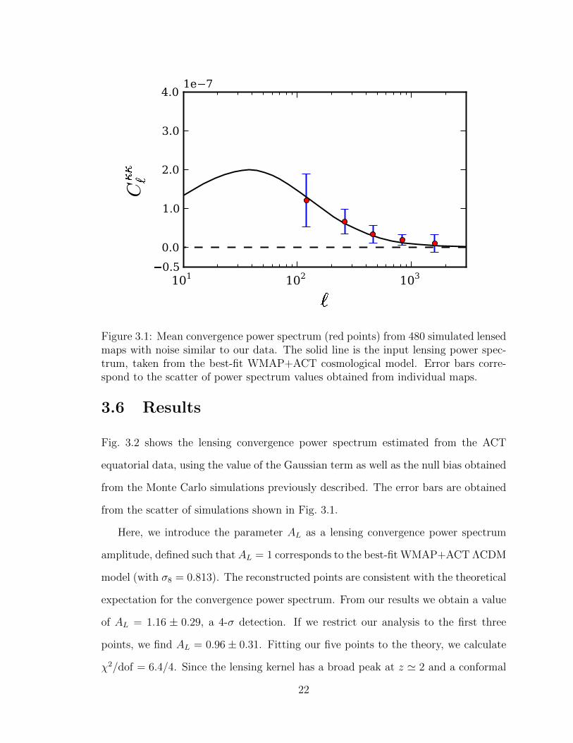
Fig. 3.2 shows the lensing convergence power spectrum estimated from the ACT

equatorial data, using the value of the Gaussian term as well as the null bias obtained

from the Monte Carlo simulations previously described. The error bars are obtained

from the scatter of simulations shown in Fig. 3.1.

Here, we introduce the parameter AL as a lensing convergence power spectrum

amplitude, defined such that AL = 1 corresponds to the best-fit WMAP+ACT ΛCDM

model (with σ8 = 0.813). The reconstructed points are consistent with the theoretical

expectation for the convergence power spectrum. From our results we obtain a value

of AL = 1.16 ± 0.29, a 4-σ detection. If we restrict our analysis to the first three

points, we find AL = 0.96 ± 0.31. Fitting our five points to the theory, we calculate

χ2/dof = 6.4/4. Since the lensing kernel has a broad peak at z ' 2 and a conformal

22

101 102 103

0.5

0.0

1.0

2.0

3.0

4.0

C

1e7

AL =1.160.29

Figure 3.2: Convergence power spectrum (red points) measured from ACT equatorialsky patches. The solid line is the power spectrum from the best-fit WMAP+ACTcosmological model with amplitude AL = 1, which is consistent with the measuredpoints. The error bars are from the Monte Carlo simulation results displayed inFig. 3.1. The best-fit lensing power spectrum amplitude to our data is AL = 1.16±0.29

distance of ' 5000 Mpc, our 4-σ detection is a direct measurement of the amplitude of

matter fluctuations at a comoving wavenumber k ∼ 0.02Mpc−1 around this redshift.

We estimate potential contamination by point sources and SZ clusters by running

our reconstruction pipeline on simulated patches which contain only IR point sources

or only thermal or kinetic SZ signal [1], while keeping the filters and the normalization

the same as for the data run. Fig. 3.3 shows that the estimated spurious convergence

power is at least two orders of magnitude below the predicted signal, due partially

to our use of only temperature modes with ` < 2300. We have also verified that

reconstruction on simulated maps containing all foregrounds (unresolved point sources

and SZ) and lensed CMB was unbiased. We found no evidence of artifacts in the

reconstructed convergence power maps.

23

Table 3.1: Reconstructed Cκκ` values.

` Range Central `b Cκκb (×10−8) σ(Cκκ

b ) (×10−8)75–150 120 19.0 6.8150–350 260 4.7 3.2350–550 460 2.2 2.3550–1050 830 4.1 1.31050–2050 1600 2.9 2.2

102 103

10-14

10-12

10-10

10-8

10-6

10-4

C

IR sources

tSZ

kSZ

Figure 3.3: Convergence power spectrum for simulated thermal and kinematic SZmaps and point source maps [1] which are a good fit to the ACT data. Note that weonly show the non-Gaussian contribution, as the Gaussian part which is of similarnegligible size is automatically included in the subtracted bias generated by phaserandomization. The solid line is the convergence power spectrum due to lensing inthe best-fit WMAP+ACT cosmological model.

24

1

0

1

2

3

4

C

(

10

7) AL =0.000.27

101 102 103

1.5

1.0

0.5

0.0

0.5

1.0

1.5

C

(

10

8) AL =0.010.02

Figure 3.4: Upper panel: Mean cross-correlation power spectrum of convergence fieldsreconstructed from different sky patches. The result is consistent with null, as ex-pected. Lower panel: Mean convergence power spectrum of noise maps constructedfrom the difference of half-season patches, which is consistent with a null signal. Theerror bars in either case are determined from Monte Carlo simulations, and those inthe lower panel are much smaller as they do not contain cosmic variance.

3.7 Null Tests

We compute a mean cross-correlation power of convergence maps reconstructed from

neighboring patches of the data map, which is expected to be zero as these patches

should be uncorrelated. We find a χ2/dof = 5.8/4 for a fit to zero signal (Fig. 3.4,

upper panel). For the second null test we construct a noise map for each sky patch

25

by taking the difference of maps made from the first half and second half of the

season’s data, and run our lensing estimator. Fig. 3.4, lower panel, shows the mean

reconstructed convergence power spectrum for these noise-only maps. Fitting to

null we calculate χ2 = 5.7 for 4 degrees of freedom. The null test is consistent

with zero, showing that the contamination of our lensing reconstruction by noise is

minimal. We also tested our phase randomization scheme by randomizing the phases

on a map, using it to reconstruct a convergence map, and cross correlating it with

a reconstruction from the same map but with a different phase randomization; our

results were consistent with null as expected.

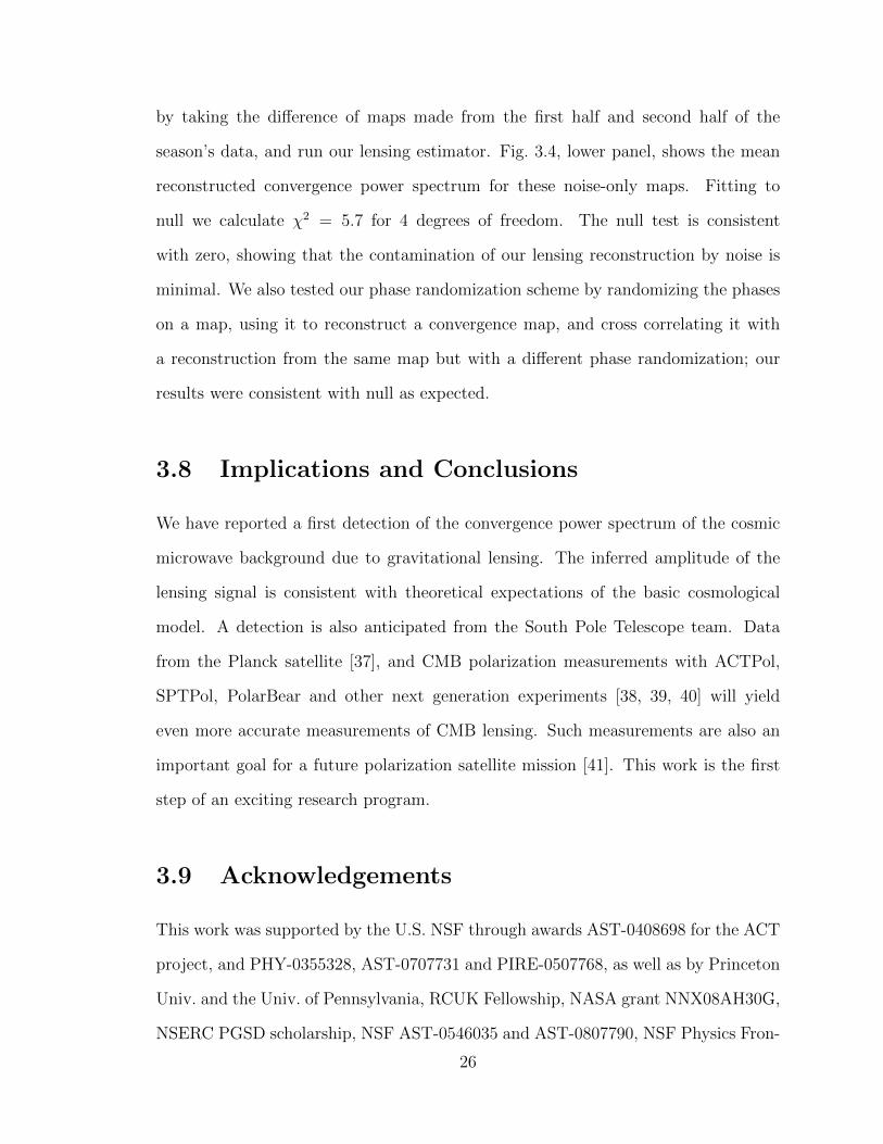
3.8 Implications and Conclusions

We have reported a first detection of the convergence power spectrum of the cosmic

microwave background due to gravitational lensing. The inferred amplitude of the

lensing signal is consistent with theoretical expectations of the basic cosmological

model. A detection is also anticipated from the South Pole Telescope team. Data

from the Planck satellite [37], and CMB polarization measurements with ACTPol,

SPTPol, PolarBear and other next generation experiments [38, 39, 40] will yield

even more accurate measurements of CMB lensing. Such measurements are also an

important goal for a future polarization satellite mission [41]. This work is the first

step of an exciting research program.

3.9 Acknowledgements

This work was supported by the U.S. NSF through awards AST-0408698 for the ACT

project, and PHY-0355328, AST-0707731 and PIRE-0507768, as well as by Princeton

Univ. and the Univ. of Pennsylvania, RCUK Fellowship, NASA grant NNX08AH30G,

NSERC PGSD scholarship, NSF AST-0546035 and AST-0807790, NSF Physics Fron-

26

tier Center grant PHY-0114422, KICP Fellowship, SLAC no.DE-AC3-76SF00515, and

the BCCP. Computations were performed on the GPC supercomputer at the SciNet

HPC Consortium. Funding at the PUC from FONDAP, Basal, and the Centre AIUC

is acknowledged. We thank B. Berger, R. Escribano, T. Evans, D. Faber, P. Gallardo,

A. Gomez, M. Gordon, D. Holtz, M. McLaren, W. Page, R. Plimpton, D. Sanchez,

O. Stryzak, M. Uehara, and the Astro-Norte group for assistance with ACT obser-

vations. We thank Thibaut Louis, Oliver Zahn and Duncan Hanson, and Kendrick

Smith for discussions and draft comments.

3.10 Addendum: Updated Measurement of the

Lensing Power Spectrum from Three Sea-

sons of Data

In this addendum we present an updated measurement of the lensing power spectrum

using improved ACT maps on the same ACT equatorial strip region. The maps used

in this analysis derive from three seasons of observations from 2008 to 2010 and

thus have significantly reduced noise levels – ' 18 µK-arcmin instead of ' 23 µK-

arcmin – as well as improvements to the mapmaking. The details of the improved

measurements, data reduction and mapmaking are described in [42].

Our new measurement of lensing uses the same methodology as previously de-

scribed in this chapter. Lensing is again measured using a quadratic estimator in

temperature; the power spectrum of the CMB lensing convergence is thus a tempera-

ture four-point function measurement, with the required filtering, normalization, and

bias subtraction performed exactly as described for the earlier measurement.

Systematic contamination of the estimator by SZ signal and IR sources was esti-

mated earlier in this chapter using the simulations from Sehgal et al. [1]. We found

27

101 102 103

ℓ

−0.5

0.0

1.0

2.0

3.0

4.0

Cκκ

ℓ

1e−7

AL =1.06±0.23

Figure 3.5: CMB convergence power spectrum reconstructed from the ACT equatorialstrip temperature data. The enhanced effective depth of the three-season coaddedACT equatorial map (' 18 µk-arcmin) compared to its previous version as describedpreviously (' 23 µk-arcmin) leads to an improved detection significance.

that, with the ACT lensing pipeline as used in this work, the contamination is smaller

than the signal by two orders of magnitude and can thus be neglected. This result

appears well-motivated for two reasons, which also apply to our updated analysis

with the improved data: first, in the analysis we only use the signal-dominated scales

below ` = 2300, at which SZ, IR and radio power are subdominant; second, by using

the data to estimate the bias, our estimator automatically subtracts the Gaussian

part of the contamination, so that only a very small non-Gaussian residual remains.

The previously described contamination estimates are not strictly applicable to this

new lensing estimate, because the filters used here contain somewhat lower noise, and

thus admit slightly more signal at higher `s; however, estimates by the SPT collabora-

tion (van Engelen et al. 2012) with similar noise levels and filters also find negligible

28

contamination. The contamination levels in our improved analysis are thus expected

to be negligible.

The measured CMB lensing power spectrum, detected at 4.6σ, is shown in Fig. 3.5,

along with a theory curve showing the convergence power spectrum for a fiducial

ΛCDM model defined by the parameter set (Ωb,Ωm,ΩΛ, h, ns, σ8) = (0.044, 0.264,

0.736, 0.71, 0.96, 0.80). Constraining the conventional lensing parameter AL that

rescales the fiducial convergence power spectrum (Cκκ` → ALC

κκ` ) we obtain AL =

1.06± 0.23. The data are thus a good fit to the ΛCDM prediction for the amplitude

of CMB lensing. We find the spectrum to have Gaussian errors, uncorrelated between

bins.

29

References

[1] Sehgal, N. et al., 2010, ApJ, 709, 920

[2] Cole, S. & Efstathiou, G., 1989, Mon. Not. R. Astron. Soc, 239, 195

[3] Linder, E. V. et al., 1990, Mon. Not. R. Astron. Soc, 243, 353

[4] Seljak, U., 1996, ApJ, 463, 1

[5] Bernardeau, F., 1997, A&A, 324, 15

[6] Zaldarriaga, M. & Seljak, U., 1999, Phys. Rev. D, 123507

[7] Hu, W. & Okamoto, T., 2002, Phys. Rev. D, 083002

[8] Challinor, A. & Lewis, A., 2003, Physics Reports, 429, 1

[9] Komatsu, E. et al., 2003, ApJS, 148, 119

[10] Spergel, D. N. et al., 2007, ApJS, 170, 377

[11] Bennett, C. L. et al., 2011, 192, 17

[12] Larson, D. et al., 2011, ApJS, 192, 16

[13] Brown, M. L. et al., 2009, ApJ, 705, 978

[14] Friedman, R. B. et al., 2009, 700, 187

[15] Reichardt, C. L. et al., 2009, ApJ, 694, 1200

30

[16] Sievers, J. L. et al., 2009, arXiv:0901.4540

[17] Lueker, M. et al., 2010, ApJ, 719, 1045

[18] Das, S. et al., 2011, ApJ, 729, 62

[19] Smith, K. M., Zahn, O., & Dore, O., 2007, Phys. Rev. D, 76, 043510

[20] Hirata, C. M., Ho, S., Padmanabhan, N., Seljak, U., and Bahcall, N. A., 2008,

Phys. Rev. D, 78, 043520

[21] Fowler, J. W. et al., 2010, ApJ, 722, 1148

[22] Swetz, D. S. et al., 2010, arXiv:1007.0290

[23] Dunkley, J. et al., 2010, arXiv:1009.0866

[24] Hajian, A., et al., 2010, arXiv:1009.0777

[25] Marriage, T. A., et al., 2010, arXiv:1007.5256

[26] Marriage, T. A., et al. 2010, arXiv:1010.1065

[27] Menanteau, F. et al., 2010, ApJ, 723, 1523

[28] Sehgal, N. et al., 2010, arXiv:1010.1025

[29] Hand, N. et al., 2011, arXiv:1101.1951

[30] Hogbom, J. A. et al., A&AS, 1974, 15, 417

[31] Hu, W. & Okamoto, T., 2002, ApJ, 574, 566

[32] Kesden, M., Cooray, A., Kamionkowski, M., 2003, Phys. Rev. D, 67, 123507

[33] Smidt, J., et al., 2011, ApJ, 728, 1

[34] Sherwin, B. D., & Das, S., 2010, arXiv:1011.4510

31

[35] Dvorkin, C., & Smith, K. M., 2009, Phys. Rev. D, 79, 043003

[36] Hanson, D., Challinor, A., Efstathiou, G., & Bielewicz, P., 2011, Phys. Rev. D,

83, 043005

[37] Perotto, L., Bobin, J., Plaszczynski, S., Starck, J., & Lavabre, A. A&A, 519, A4

[38] Niemack, M. D. et al., 2010, SPIE Conference Series, 7741

[39] McMahon, J. J. et al., 2009, in AIP Conference Series, 1185

[40] Lee, A. T., et al., 2008, in AIP Conference Series, 1040

[41] Smith, K. M. et al., 2008, arXiv:0811.3916

[42] Das, S. et al., 2013, arXiv:1301.1037

32

Chapter 4

Evidence for Dark Energy from the

CMB Alone Using ACT Lensing

Measurements

4.1 Abstract

For the first time, measurements of the cosmic microwave background radiation

(CMB) alone favor cosmologies with w = −1 dark energy over models without dark

energy at a 3.2-sigma level. We demonstrate this by combining the CMB lensing

deflection power spectrum from the Atacama Cosmology Telescope with temperature

and polarization power spectra from the Wilkinson Microwave Anisotropy Probe.

The lensing data break the geometric degeneracy of different cosmological models

with similar CMB temperature power spectra. Our CMB-only measurement of the

dark energy density ΩΛ confirms other measurements from supernovae, galaxy clus-

ters and baryon acoustic oscillations, and demonstrates the power of CMB lensing as

a new cosmological tool.

33

4.2 Introduction

Observations made over the past two decades suggest a standard cosmological model

for the contents and geometry of the universe, as well as for the initial fluctuations that

seeded cosmic structure [4, 5, 6]. The data imply that our universe at the present

epoch has a dominant stress-energy component with negative pressure, known as

“dark energy”, and has zero mean spatial curvature. The cosmic microwave back-

ground (CMB) has played a crucial role in constraining the fractional energy densities

in matter, Ωm, and in dark energy or the cosmological constant, ΩΛ (or equivalently

in curvature ΩK = 1− ΩΛ − Ωm) [e.g., 33]. Throughout this chapter, we restrict our

analysis to the simplest dark energy models with equation of state parameter w = −1.

The existence of dark energy, first directly observed by supernova measurements

[4, 5], is required [6] by the combination of CMB power spectrum measurements and

any one of the following low redshift observations [10, 11, 13, 14, 12]: measurements

of the Hubble constant, measurements of the galaxy power spectrum, galaxy cluster

abundances, or supernova measurements of the redshift-distance relation. At present,

the combination of low-redshift astronomical observations with CMB data can con-

strain cosmological parameters in a universe with both vacuum energy and curvature

to better than a few percent [33].

However, from the CMB alone, it has not been possible to convincingly demon-

strate the existence of a dark energy component, or that the universe is geometrically

flat [6, 33]. This is due to the “geometric degeneracy” which prevents both the curva-

ture and expansion rate from being determined simultaneously from the CMB alone

[1, 2, 3]. The degeneracy can be understood as follows. The first peak of the CMB

temperature power spectrum measures the angular size of a known physical scale:

the sound horizon at decoupling, when the CMB was last scattered by free electrons.

However, very different cosmologies can project this sound horizon onto the same

degree-scale angle on the sky: from a young universe with a large vacuum energy and

34

negative spatial curvature, to the standard spatially flat cosmological model, to an

old universe with no vacuum energy, positive spatial curvature, and a small Hubble

constant [22]. These models, therefore, cannot be significantly distinguished using

only primordial CMB power spectrum measurements.

By observing the CMB at higher resolution, however, one can break the geometric

degeneracy using the effect of gravity on the CMB [20]: the deflection of CMB photons

on arcminute scales due to gravitational lensing by large scale structure. This lensing

of the CMB can be described by a deflection field d(n) which relates the lensed and

unlensed temperature fluctuations δT, δT in a direction n as δT (n) = δT (n + d).

The lensing signal, first detected at 3.4σ from the cross-correlation of radio sources

with WMAP data [23] and at 4σ from the CMB alone by the Atacama Cosmology

Telescope (ACT) [7], is sensitive to both the growth of structure in recent epochs and

the geometry of the universe [1]. Combining the low-redshift information from CMB

lensing with CMB power spectrum data gives significant constraints on ΩΛ, which

the power spectrum alone is unable to provide.

The constraining power of the CMB lensing measurements is apparent in a com-

parison between two models consistent with the CMB temperature power spectrum

(see Fig. 4.1): the spatially flat ΛCDM model with dark energy which best fits the

WMAP seven-year data [24] and a model with positive spatial curvature but without

dark energy.

The two theory temperature spectra and the temperature-polarization cross-

correlation spectra differ only at the largest scales with multipoles ` < 10, where the

cosmic variance errors are large. (The differences are due to the Integrated Sachs-

Wolfe (ISW) effect, a large-scale CMB distortion induced by decaying gravitational

potentials in the presence of dark energy [17] or, with the opposite sign, induced by

growing potentials in the presence of positive curvature.) Though the temperature-

35

100 101 102 103

1000

0

1000

2000

3000

4000

5000

6000

(

+1)C

/2

[K2]

CDM

=0

WMAP

101 102 103

0.5

0.0

0.5

1.0

1.5

2.0

2.5

3.0

3.5

4.0

2C

dd

/4

1e7

CDM

=0

ACT

Figure 4.1: Upper panel: Angular power spectra of CMB temperature fluctuationsfor two geometrically degenerate cosmological models, one the best-fit curved uni-verse with no vacuum energy (ΩΛ = 0,Ωm = 1.29), and one the best-fit flat ΛCDMmodel with ΩΛ = 0.73,Ωm = 0.27. The seven-year WMAP temperature power spec-trum data [24] are also shown; they do not significantly favor either model. Lowerpanel: The CMB lensing deflection power spectra are shown for the same two models.They are no longer degenerate: the ΩΛ = 0 universe would produce a lensing powerspectrum larger than that measured by ACT ([7], also shown above).

36

polarization cross-spectra differ somewhat at low `, overall the polarization spectra

in the two models are also very similar on all scales.

However, these two cosmologies predict significantly different CMB lensing deflec-

tion power spectra Cdd` . Fig. 4.1 shows that the universe with ΩΛ = 0 produces more

lensing on all scales. The ACT measurements shown in Fig. 4.1 are a better fit to the

model with vacuum energy than to the model without dark energy.

Why is the lensing power spectrum higher in a universe without dark energy

but with the same primordial CMB spectrum? This can be understood from the

expression for the power spectrum of lensing deflection angles [1]:

`2

4C`

dd =

∫ η∗

0

dη W 2(η)︸ ︷︷ ︸geometry

[D (η) /a(η)]2︸ ︷︷ ︸growth

(4.1)

where η is conformal lookback distance, η∗ is the conformal distance to the CMB last

scattering surface, D is the growth factor of matter perturbations since decoupling,

a is the scale factor, and W (η) is a geometry and projection term given by

W (η) =3

2ΩmH

20

dA(η∗ − η)

dA(η∗)P 1/2

(k =

`+ 1/2

dA(η), η∗

).

where H0 is the Hubble constant, dA is comoving angular diameter distance, P (k, η∗)

is the matter power spectrum at decoupling and k is the comoving wavenumber.

A plot of the kernel of the lensing integral in this equation, as well as its constituent

“geometry” and “growth” terms, is shown in Fig. 4.2 for both ΛCDM and ΩΛ = 0

models. This figure shows that increased lensing in universes without dark energy is

due to three effects: (1) CMB photons in a universe without dark energy spend more

time at lower redshifts where structure is larger; (2) structure and potentials grow

more in a universe with ΩΛ = 0 and positive curvature; (3) in a universe without dark

energy, projection effects pick out longer wavelength fluctuations which are larger for

most lensing scales.

37

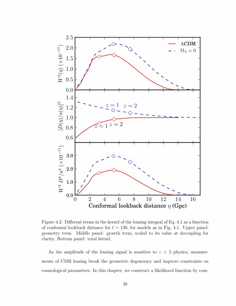
Figure 4.2: Different terms in the kernel of the lensing integral of Eq. 4.1 as a functionof conformal lookback distance for ` = 120, for models as in Fig. 4.1. Upper panel:geometry term. Middle panel: growth term, scaled to its value at decoupling forclarity. Bottom panel: total kernel.

As the amplitude of the lensing signal is sensitive to z < 5 physics, measure-

ments of CMB lensing break the geometric degeneracy and improve constraints on

cosmological parameters. In this chapter, we construct a likelihood function by com-

38

bining ACT lensing measurements and WMAP power spectra, and explore the new

CMB-only parameter constraints resulting from the inclusion of lensing data.

4.3 Methodology

We fit a joint distribution for a set of cosmological parameters θ to our data D (see,

e.g. [24]). In our analysis, we consider the following cosmological parameters:

θ = ΩΛ,ΩK ,Ωbh2,Ωch

2, ns,∆2R, τ, ASZ (4.2)

where Ωbh2 is the baryon density, Ωch

2 is the cold dark matter (CDM) density,

ns is the spectral tilt of the density fluctuations, ∆2R is their amplitude (defined

at pivot scale k0 = 0.002/Mpc), τ is the optical depth to reionization, and ASZ

is the amplitude of the WMAP V-band SZ template [31]. The Hubble constant,

H0 ≡ 100 h km/s/Mpc, can be derived from these parameters. The estimated dis-

tribution is the product of the likelihood p(D|C`(θ)) and the prior p(θ). Here C`(θ)

is the set of theoretical angular power spectra (CMB temperature power spectrum

CTT` , CMB polarization power spectra CTE

` and CEE` , and lensing deflection angle

power spectrum Cdd` ) derived from the parameters θ. Uniform priors are placed on all

sampled parameters. We use data from the WMAP seven-year temperature and po-

larization observations [24], which map the CMB anisotropy over the full sky. These

are combined with the ACT lensing deflection power spectrum described in [7], ob-

tained from a measurement of the lensing non-Gaussianity in a 324 deg2 patch of

the ACT equatorial CMB maps. The data were found to be effectively free of con-

tamination from astrophysical sources or noise, with errors that were estimated to

be Gaussian and uncorrelated. Since the correlation between the datasets is negligi-

ble, the likelihood is the product of the WMAP likelihood, p(DWMAP|C`TT,TE,EE(θ)),

described in [24], and the ACT lensing likelihood, p(DACT|C`dd(θ)) [7].

39

Theoretical CMB temperature and lensing power spectra are computed using the

CAMB code [26]. We follow the same approach as [22, 24] to map out the posterior

distribution of the parameters.

4.4 Results

The two-dimensional marginalized distribution for ΩΛ and Ωm = 1−ΩK−ΩΛ is shown

in Fig. 4.3, with 68% and 95% confidence levels, indicating the effect of adding the

ACT lensing data.

The distribution for WMAP alone is limited by the ISW effect in both the TE

and TT power, but is still unbounded at ΩΛ = 0. It is truncated with the addition

of the lensing data, resulting in a two-dimensional 95% confidence level that excludes

ΩΛ = 0. The one-dimensional probability density for ΩΛ, shown in Fig. 4.4, further

demonstrates how the CMB lensing data reduce the low-ΩΛ tail of the probability

distribution and break the geometric degeneracy. A universe without dark energy

would give too large a lensing signal to be consistent with the data. With lensing

data, the new confidence intervals for ΩΛ are 0.61+0.14−0.06 at 1σ (68% C.L.), 0.61+0.23

−0.29 at

2σ (95% C.L.) and 0.61+0.25−0.53 at 3σ (99.7% C.L.), favoring a model with dark energy.

Comparing the likelihood value for the best-fit ΛCDM model with the likelihood for

the best-fit ΩΛ = 0 model, we find that ΩΛ = 0 is disfavored at 3.2σ (∆χ2 ≈ 11,

of which ∆χ2 ≈ 5 arises from the WMAP spectra, mainly due to differences in the

TE and TT power spectra for ` < 10). The parameters of the best-fit ΛCDM model

are consistent with constraints from other datasets such as the WMAP+BAO+H0

constraints of [33]. The effect of massive neutrinos on the lensing spectrum is different

from the effect of ΩΛ; neutrino masses within the current bounds can only modify

the shape of the spectrum by < 5% [30], whereas the reduction in ΩΛ considered here

increases the spectrum on all scales by a much larger amount.

40

0.0 0.2 0.4 0.6 0.8 1.0 1.2

ΩM

0.0

0.2

0.4

0.6

0.8

1.0

ΩΛ

ΩK =0

without ACT-Lensing

Figure 4.3: Two-dimensional marginalized posterior probability for Ωm and ΩΛ (68%and 95% C.L.s shown). Colored contours are for WMAP + ACT Lensing, black linesare for WMAP only. Using WMAP data alone, universes with ΩΛ = 0 lie within the95% C.L. The addition of lensing data breaks the degeneracy, favoring models withdark energy.

4.5 Conclusions

We find that a dark energy component ΩΛ is required at a 3.2σ level from CMB data

alone. This constraint is due to the inclusion of CMB lensing power spectrum data,

which probe structure formation and geometry long after decoupling and so break

the CMB geometric degeneracy. Our analysis provides the first demonstration of the

ability of the CMB lensing power spectrum to constrain cosmological parameters. It

provides a clean verification of other measurements of dark energy. In future work,

our analysis can be easily extended to give constraints on more complex forms of

dark energy with w 6= −1. With much more accurate measurements of CMB lensing

41

0.0 0.2 0.4 0.6 0.8 1.0

ΩΛ

0.0

0.2

0.4

0.6

0.8

1.0p(Ω

Λ)

WMAP

WMAP + ACT-Lensing

Figure 4.4: One-dimensional marginalized posterior probability for ΩΛ (not normal-ized). An energy density of ΩΛ ' 0.7 is preferred even from WMAP alone, but whenlensing data are included, an ΩΛ = 0 universe is strongly disfavoured.

expected from ACT, SPT [27], Planck [28], and upcoming polarization experiments

including ACTPol [29], lensing reconstruction promises to further elucidate the prop-

erties of dark energy and dark matter [32].

4.6 Acknowledgements

This work was supported by the U.S. NSF through awards AST-0408698, PHY-

0355328, AST-0707731 and PIRE-0507768, as well as by Princeton Univ., the Univ.

of Pennsylvania, FONDAP, Basal, Centre AIUC, RCUK Fellowship, NASA grant

NNX08AH30G, NSERC PGSD, the Rhodes Trust, NSF AST-0546035 and AST-

0807790, NSF PFC grant PHY-0114422, KICP Fellowship, SLAC no. DE-AC3-

76SF00515, ERC grant 259505, BCCP, and the NSF GRFP. We thank B. Berger,

R. Escribano, T. Evans, D. Faber, P. Gallardo, A. Gomez, M. Gordon, D. Holtz, M.

McLaren, W. Page, R. Plimpton, D. Sanchez, O. Stryzak, M. Uehara, and Astro-

42

Norte for assistance with ACT. ACT operates in the Parque Astronomico Atacama

in northern Chile under the auspices of Programa de Astronomıa, a program of the

Comision Nacional de Investigacion Cientıfica y Tecnologica de Chile (CONICYT).

We thank Alex van Engelen for discussions and thank Matias Zaldarriaga and Duncan

Hanson for comments on the draft.

43

References

[1] Doroshkevich, A. G., Zel’dovich, Y. B. & Sunyaev, R. A. 1978, Soviet Astronomy,

22, 523

[2] Bond, J. R., Efstathiou, G. & Tegmark, M., 1997, Mon. Not. R. Astron. Soc, 291,

L33

[3] Zaldarriaga, M., Spergel, D. N. & Seljak, U., 1997, ApJ, 488, 1

[4] Riess, A. G. et al. , 1998, AJ, 116, 1009

[5] Perlmutter S. et al., 1999, ApJ, 517, 565

[6] Spergel D. N. et al., 2003, ApJS, 148, 175

[7] Smoot G. F. et al., 1992, ApJ, 396, L1

[8] Miller A. D. et al., 1999, ApJ, 524, L1

[9] Komatsu E. et al., 2009, ApJS, 180, 330

[10] Hicken, M. et al., 2009, 700, 1097

[11] Kessler, R. et al., 2009, ApJS, 185, 32

[12] Vikhlinin, A. et al., 2009, ApJ, 692, 1060

[13] Reid, B. A. et al., 2010, Mon. Not. R. Astron. Soc, 404, 60

44

[14] Riess, A. G. et al., 2009, ApJ, 699, 539

[15] Das, S. et al., 2011, PRL in press

[16] Komatsu, E. et al., 2010, ApJS

[17] Boughn, S. P., Crittenden, R. G. & Turok, N. G., 1998, New Astronomy, 3, 275

[18] Boughn, S. & Crittenden, R., 2004, Nature, 427, 45

[19] Lewis, A. & Challinor, A., 2006, 429, 1

[20] Stompor, R. & Efstathiou, G., 1999, Mon. Not. R. Astron. Soc, 302, 735

[21] Zaldarriaga, M. & Seljak, U., 1998, Phys. Rev. D, 58, 023003

[22] Dunkley, J. et al., 2009, 180, 306

[23] Smith, K. M., Zahn, O. & Dore, O., 2007, 76, 043510

[24] Larson, D. et al., 2010, arxiv

[25] Dunkley, J. et al., 2010, arXiv:1009.0866D

[26] Lewis, A., Challinor, A. & Lasenby, A., 2000, ApJ, 658, 473

[27] Carlstrom, J. E. et al., 2009, arXiv:0907.4445C

[28] Perotto, L. et al., 2010, A&A, 519, A4

[29] Niemack, M. D. et al., 2010, Proc. SPIE, 7741

[30] Lesgourgues, J., Perotto, L., Pastor, S. & Piat, M., 2006, Phys. Rev. D, 73, 4

[31] Komatsu, E. & Seljak, U., 2002, Mon. Not. R. Astron. Soc, 336, 1256

[32] Galli, S. et al., 2010, Phys. Rev. D, 82, 123504

[33] Komatsu, E. et al., ApJS, 192, 18

45

Chapter 5

Cross-correlation of CMB Lensing

with the Distribution of Quasars

5.1 Abstract

We measure the cross-correlation of Atacama Cosmology Telescope CMB lensing

convergence maps with quasar maps made from the Sloan Digital Sky Survey DR8

SDSS-XDQSO photometric catalog. The CMB lensing-quasar cross-power spectrum

is detected for the first time at a significance of 3.8σ, which directly confirms that

the quasar distribution traces the mass distribution at high redshifts z > 1. Our

detection passes a number of null tests and systematic checks. Using this cross-power

spectrum, we measure the amplitude of the linear quasar bias assuming a template

for its redshift dependence, and find the amplitude to be consistent with an earlier

measurement from clustering; at redshift z ≈ 1.4, the peak of the distribution of

quasars in our maps, our measurement corresponds to a bias of b = 2.5 ± 0.6. With

the signal-to-noise ratio on CMB lensing measurements likely to improve by an order

of magnitude over the next few years, our results demonstrate the potential of CMB

lensing cross-correlations to probe astrophysics at high redshifts.

46

5.2 Introduction

As the photons of the cosmic microwave background (CMB) travel through the uni-

verse, they are gravitationally deflected by the web of matter through which they pass.

In the CMB sky we observe today, these deflections are imprinted as arcminute-scale

distortions of small scale temperature fluctuations [1, 2]. The microwave background

thus contains not only information about the primordial universe at redshift ≈ 1100,

but also about the matter density fluctuations in the lower redshift universe.

CMB lensing measurements are a powerful cosmological probe [10] because they

are sensitive to both the growth of density fluctuations and the geometry and size

of the universe, yet are relatively insensitive to both instrumental and astrophysical

systematic errors [6, 7]. Lensing measurements can constrain the properties of dark

energy [18], the amplitude of density fluctuations and the masses of neutrinos [11].

They can also constrain the properties of biased tracers of the matter distribution.

The focus of this chapter is the cross-correlation of CMB lensing maps with one such

tracer – quasars.

Quasars are among the most luminous objects in the universe. Their immense

luminosity is believed to be powered by accreting supermassive black holes [12, 13]

which reside at the center of almost every massive galaxy [14]. As the activity of

quasars and the rate of star formation appear to be linked [15], they are a crucial

element in our present understanding of galaxy evolution. Measurements of the rela-

tion between dark matter and the distribution of quasars can inform us about quasar

properties such as the masses of the dark matter halos that host the quasars, the

scatter in the quasar-halo mass relation and the quasar duty cycle (see e.g. [16]).

Such measurements of quasar properties will, in turn, improve our understanding of

structure formation and galaxy evolution.

Both the number density of quasars and the strength of CMB lensing in a certain

direction depend on the projected dark matter density in this direction, and quasars

47

are most common at the redshifts that produce the largest lensing deflections. This

implies that the CMB lensing and quasar fields should be strongly correlated [17].

Measuring the cross-power spectrum and comparing it to theoretical calculations, we

can determine the proportionality factor which relates a fluctuation in matter density

to a fluctuation in quasar number density. This proportionality factor is known as

the quasar linear bias b (defined as b ≡ δq/δ where δq and δ are the fractional spatial

overdensities of quasars and matter respectively).

In this work we present the first measurement of the CMB lensing-quasar cross-

power spectrum, and use it to derive a constraint on the quasar bias. The chapter

is organized as follows. Section II presents the theoretical background underlying

the CMB lensing-quasar cross-correlation. Section III explains how the lensing and

quasar maps used in our analysis are constructed, and describes the resulting cross-

spectrum measurement. The constraint on quasar linear bias we obtain from the

cross-power spectrum is presented in section IV. Null tests and systematic checks are

discussed in section V. All calculations assume a ΛCDM cosmology with WMAP5

parameters [19] and σ8 = 0.819.

5.3 Theoretical Background

Cosmological weak lensing effects can be described using the convergence field κ,

which is equal to a weighted projection of the matter overdensity δ [1]

κ(n) =

∫ zLS

0

dzW κ(z)δ(η(z)n, z). (5.1)

The relevant kernel (assuming a flat universe) is

W κ(z) =3

2H(z)Ω0H

20 (1 + z)η(z)

(ηLS − η(z)

)ηLS

(5.2)

48

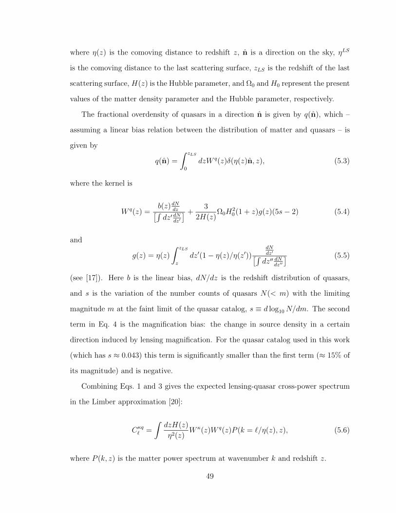
where η(z) is the comoving distance to redshift z, n is a direction on the sky, ηLS

is the comoving distance to the last scattering surface, zLS is the redshift of the last

scattering surface, H(z) is the Hubble parameter, and Ω0 and H0 represent the present

values of the matter density parameter and the Hubble parameter, respectively.

The fractional overdensity of quasars in a direction n is given by q(n), which –

assuming a linear bias relation between the distribution of matter and quasars – is

given by

q(n) =

∫ zLS

0

dzW q(z)δ(η(z)n, z), (5.3)

where the kernel is

W q(z) =b(z)dN

dz[∫dz′ dN

dz′

] +3

2H(z)Ω0H

20 (1 + z)g(z)(5s− 2) (5.4)

and

g(z) = η(z)

∫ zLS

z

dz′(1− η(z)/η(z′))dNdz′[∫dz′′ dN

dz′′

] (5.5)

(see [17]). Here b is the linear bias, dN/dz is the redshift distribution of quasars,

and s is the variation of the number counts of quasars N(< m) with the limiting

magnitude m at the faint limit of the quasar catalog, s ≡ d log10N/dm. The second

term in Eq. 4 is the magnification bias: the change in source density in a certain

direction induced by lensing magnification. For the quasar catalog used in this work

(which has s ≈ 0.043) this term is significantly smaller than the first term (≈ 15% of

its magnitude) and is negative.

Combining Eqs. 1 and 3 gives the expected lensing-quasar cross-power spectrum

in the Limber approximation [20]:

Cκq` =

∫dzH(z)

η2(z)W κ(z)W q(z)P (k = `/η(z), z), (5.6)

where P (k, z) is the matter power spectrum at wavenumber k and redshift z.

49

5.4 Cross-correlating CMB Lensing and Quasars

5.4.1 The ACT CMB Lensing Convergence Maps

The lensing convergence fields used in our analysis are reconstructed from CMB

temperature maps made by the Atacama Cosmology Telescope (ACT) [23, 24, 25],

a 6m telescope operating in the Atacama desert in Chile. These CMB temperature

maps are obtained from observations made during 2008-2010 in the 148 GHz frequency

band and calibrated as in [26]. The maps consist of six patches, each of size 3 × 18

degrees, in the Sloan Digital Sky Survey (SDSS) Stripe 82 region [27], with a map-

averaged white noise level of 21 µK arcmin. Radio and IR point sources as well as

Sunyaev-Zel’dovich (SZ) clusters detected with a matched filter at a signal-to-noise

ratio greater than 5 as in [6] are masked and inpainted using the methods of [9].

The convergence maps are reconstructed from the CMB temperature maps as in

[6] using the minimum variance quadratic estimator procedure described in [3]. The

estimator works as follows. While the unlensed CMB is statistically isotropic, any

lensing deflection imprints a preferred direction into the statistical properties of the

CMB. This corresponds mathematically to the fact that formerly uncorrelated modes

of the isotropic unlensed CMB temperature field are correlated by lensing, with the

correlation proportional to the lensing deflection. We can hence estimate the lensing

convergence by measuring the correlation between pairs of Fourier modes using a

quadratic estimator:

κ(L) = N(L)

∫d2l f(L, l) T (l)T (L− l). (5.7)

Here l,L are Fourier space coordinates, N is the normalization function (which ensures

that the estimator is unbiased) and f is a weighting such that the signal-to-noise

ratio on the reconstructed convergence is maximized in the case of isotropic noise

50

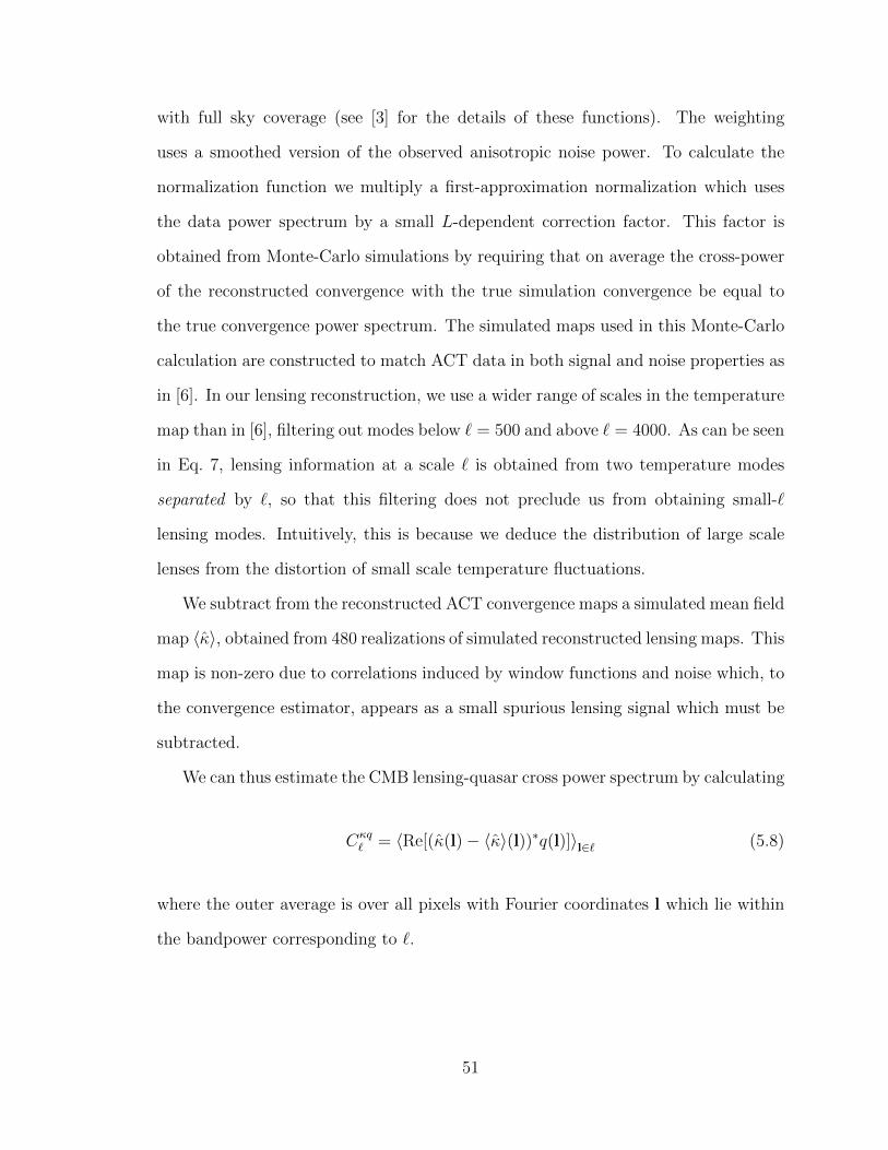
with full sky coverage (see [3] for the details of these functions). The weighting

uses a smoothed version of the observed anisotropic noise power. To calculate the

normalization function we multiply a first-approximation normalization which uses

the data power spectrum by a small L-dependent correction factor. This factor is

obtained from Monte-Carlo simulations by requiring that on average the cross-power

of the reconstructed convergence with the true simulation convergence be equal to

the true convergence power spectrum. The simulated maps used in this Monte-Carlo

calculation are constructed to match ACT data in both signal and noise properties as

in [6]. In our lensing reconstruction, we use a wider range of scales in the temperature

map than in [6], filtering out modes below ` = 500 and above ` = 4000. As can be seen

in Eq. 7, lensing information at a scale ` is obtained from two temperature modes

separated by `, so that this filtering does not preclude us from obtaining small-`

lensing modes. Intuitively, this is because we deduce the distribution of large scale

lenses from the distortion of small scale temperature fluctuations.

We subtract from the reconstructed ACT convergence maps a simulated mean field

map 〈κ〉, obtained from 480 realizations of simulated reconstructed lensing maps. This

map is non-zero due to correlations induced by window functions and noise which, to

the convergence estimator, appears as a small spurious lensing signal which must be

subtracted.

We can thus estimate the CMB lensing-quasar cross power spectrum by calculating

Cκq` = 〈Re[(κ(l)− 〈κ〉(l))∗q(l)]〉l∈` (5.8)

where the outer average is over all pixels with Fourier coordinates l which lie within

the bandpower corresponding to `.

51

0.0 0.5 1.0 1.5 2.0 2.5 3.0 3.5 4.0z

0.0

0.2

0.4

0.6

0.8

1.0dN/dz

0.0 0.5 1.0 1.5 2.0 2.5 3.0 3.5 4.00.0

0.2

0.4

0.6

0.8

1.0

W

Figure 5.1: The redshift distribution of SDSS quasars used to construct our mapsof fractional quasar overdensity, normalized to a unit maximum. The correspondingredshift bins are shown with blue filled circles; they are interpolated to give the con-tinuous curve used in our theory calculations (blue dashed line). For comparison, thered dotted line shows the lensing kernel W κ(z), again normalized to a unit maximum.

5.4.2 The SDSS Quasar Maps

In this work we use the SDSS-XDQSO photometric quasar catalog [21, 22], extracted

from the SDSS Data Release 8. The analysis used in this catalog separates the popu-

lation of quasars and foreground stars using a probabilistic model in flux space. This

analysis assigns a probability of being a quasar to every point-source with de-reddened

i-band magnitude between 17.75 and 22.45 mag in the SDSS imaging. Though the

catalog extends out to z > 4, we do not use the highest-redshift sources with redshifts

z > 3.5. This reduces the shot noise error on our measurement, as there are very few

such sources. Using this catalog, we construct a map of the fractional overdensity q

of quasars across the same 324 square degrees on which we perform our lensing recon-

struction. We include in our quasar maps, with unit weight, all point sources with a

52

greater than p = 0.68 probability of being a quasar. As the probability distribution

is non-uniform, the residual level of stellar contamination can be calculated from the

catalog probabilities to be 6% (we discuss later how this is accounted for in our theo-

retical calculations). A spectroscopic quasar sample at high redshifts (2.2 < z < 3.5)

does show a contamination fraction which is ≈ 15% larger than that predicted by

the catalog (see [22]); however, the majority of the quasars we consider are at lower

redshift where the XDQSO model estimates should be significantly more accurate

(high redshift quasar selection is less accurate because at z ≈ 2.8 the quasar and

stellar loci cross in color space). We neglect the error on the stellar contamination

fraction, which is any case smaller than the statistical error (and would only reduce

the measured signal, not increase it). The area covered by our quasar maps contains

on average 75 quasars per square degree. The redshift distribution of the quasars in

our maps is shown in Fig. 1, along with the CMB lensing kernel, which has a very

similar redshift distribution.

5.4.3 The CMB Lensing - Quasar Cross-Power Spectrum

The cross-power spectrum of the ACT CMB lensing maps and the SDSS quasar maps

is shown in Fig. 2.

The error bars on the data points are calculated theoretically as proportional to√Cκκ` Cqq

` , with an additional factor calculated from the number of independent pixels

in the bin corresponding to each data point. The spectra used in this calculation are

the full data spectra which include both signal and noise (including Poisson noise).

Bootstrap error estimates from splits of our data are consistent with this calculation.

For comparison, we also calculate error bars using Monte-Carlo methods, cross cor-

relating 480 realizations of simulated reconstructed lensing maps (containing signal

and realistic noise) with the quasar data maps. Both methods assume the two maps

are uncorrelated; such calculations are very good approximations to the true error

53

0 500 1000 1500 2000

0

1

2

3

4

C

q

107

Figure 5.2: The CMB lensing - quasar density cross-power spectrum, with the datapoints shown in blue (the covariance between different data points is negligible).The significance of the detection of the cross-spectrum is 3.8σ. The green solid lineis a theory line calculated assuming the fiducial bias amplitude. This theory line isreduced by 6% to account for the expected level of stellar contamination of the quasarsample.

on the cross-correlation because both maps are noisy so that Cκκ` Cqq

` (Cκq` )2. The

error bars obtained from Monte-Carlo methods are nearly indistinguishable from the

theory error bars, and lead to the same detection significance. (We also verified that

replacing the quasar data maps with 480 simulated maps with the same number of

randomly distributed sources leads to similar, though slightly smaller, errors.) The

Monte-Carlo estimates of the errors also allow us to calculate the full covariance ma-

trix. The off-diagonal elements are negligible compared to the diagonal elements;

for every bin, the covariance between neighboring bins was less than 4% of the bin

autocorrelation. We thus neglect covariance between different data points in our

analysis.

54

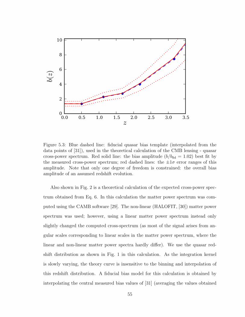
0.0 0.5 1.0 1.5 2.0 2.5 3.0 3.5z

0

2

4

6

8

10

b(z)

Figure 5.3: Blue dashed line: fiducial quasar bias template (interpolated from thedata points of [31]), used in the theoretical calculation of the CMB lensing - quasarcross-power spectrum. Red solid line: the bias amplitude (b/bfid = 1.02) best fit bythe measured cross-power spectrum; red dashed lines: the ±1σ error ranges of thisamplitude. Note that only one degree of freedom is constrained: the overall biasamplitude of an assumed redshift evolution.

Also shown in Fig. 2 is a theoretical calculation of the expected cross-power spec-

trum obtained from Eq. 6. In this calculation the matter power spectrum was com-

puted using the CAMB software [29]. The non-linear (HALOFIT, [30]) matter power

spectrum was used; however, using a linear matter power spectrum instead only

slightly changed the computed cross-spectrum (as most of the signal arises from an-

gular scales corresponding to linear scales in the matter power spectrum, where the

linear and non-linear matter power spectra hardly differ). We use the quasar red-

shift distribution as shown in Fig. 1 in this calculation. As the integration kernel

is slowly varying, the theory curve is insensitive to the binning and interpolation of

this redshift distribution. A fiducial bias model for this calculation is obtained by

interpolating the central measured bias values of [31] (averaging the values obtained

55

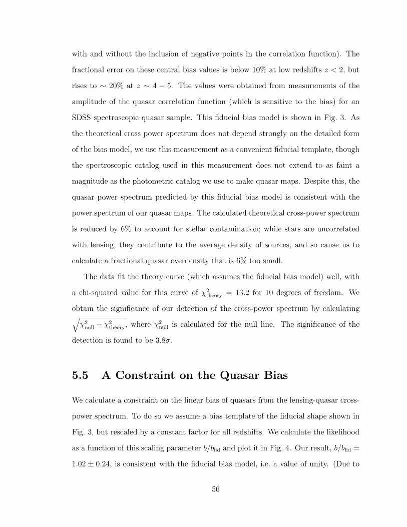
with and without the inclusion of negative points in the correlation function). The

fractional error on these central bias values is below 10% at low redshifts z < 2, but

rises to ∼ 20% at z ∼ 4 − 5. The values were obtained from measurements of the

amplitude of the quasar correlation function (which is sensitive to the bias) for an

SDSS spectroscopic quasar sample. This fiducial bias model is shown in Fig. 3. As

the theoretical cross power spectrum does not depend strongly on the detailed form

of the bias model, we use this measurement as a convenient fiducial template, though

the spectroscopic catalog used in this measurement does not extend to as faint a

magnitude as the photometric catalog we use to make quasar maps. Despite this, the

quasar power spectrum predicted by this fiducial bias model is consistent with the

power spectrum of our quasar maps. The calculated theoretical cross-power spectrum

is reduced by 6% to account for stellar contamination; while stars are uncorrelated

with lensing, they contribute to the average density of sources, and so cause us to

calculate a fractional quasar overdensity that is 6% too small.

The data fit the theory curve (which assumes the fiducial bias model) well, with

a chi-squared value for this curve of χ2theory = 13.2 for 10 degrees of freedom. We

obtain the significance of our detection of the cross-power spectrum by calculating√χ2

null − χ2theory, where χ2

null is calculated for the null line. The significance of the

detection is found to be 3.8σ.

5.5 A Constraint on the Quasar Bias

We calculate a constraint on the linear bias of quasars from the lensing-quasar cross-

power spectrum. To do so we assume a bias template of the fiducial shape shown in

Fig. 3, but rescaled by a constant factor for all redshifts. We calculate the likelihood

as a function of this scaling parameter b/bfid and plot it in Fig. 4. Our result, b/bfid =

1.02 ± 0.24, is consistent with the fiducial bias model, i.e. a value of unity. (Due to

56

the small negative magnification bias, b/bfid = 0 does not correspond exactly to the

null line.) As the redshift distribution is peaked at z = 1.4, b/bfid can be interpreted

as approximately parametrizing the amplitude of the bias at redshift 1.4. From this

interpretation we obtain a value of the bias at z ≈ 1.4 of b = 2.5 ± 0.6, which is

in good agreement with previous measurements from quasar clustering [31]. We can

associate this bias with a host halo mass M200: using the bias model of [32], we

obtain a halo mass of log10(M200/M) = 12.9+0.3−0.5, consistent with previous estimates

[31, 16]. We also verify that the cross-power calculated using only a low (z < 2.2)

or high (z > 2.2) redshift quasar sub-sample is consistent with the bias given by

the fiducial model; however, we defer a detailed calculation of bias constraints using

multiple quasar sub-samples to future work with a higher signal-to-noise ratio.

0.0 0.5 1.0 1.5 2.0

b/bfid

0.0

0.2

0.4

0.6

0.8

1.0

likelihood

Figure 5.4: Likelihood as a function of quasar bias divided by the fiducial bias,b/bfid (we assume that the shape of the redshift dependence is constant and has thefiducial form of Fig. 3, and modify the amplitude of the bias function to calculate thislikelihood.) Interpreting our measurement of b/bfid = 1.02± 0.24 as a bias at z ≈ 1.4(the peak in the quasar distribution), we obtain b = 2.5± 0.6 at this redshift.

57

5.6 Testing the power spectrum

5.6.1 Null Tests

We check our result and our pipeline with a number of null tests. In a simple first

test, we cross-correlate the quasar distribution in one part of the sky with the lensing

convergence in another; as seen in Fig. 5, the results are consistent with null as ex-

pected, with χ2 = 6.5 for 10 degrees of freedom for a fit to null. A more sophisticated

test is to calculate the cross-correlation of the quasar maps with the curl component

of the lensing deflection (this differs from the convergence reconstructed earlier, which

is gradient-like). The reconstructed curl map is expected to be zero (though it should

contain reconstruction noise), and hence the cross-correlation with the quasar maps

should be zero as well. We reconstruct the curl component of the estimator as in [7]

(though keeping the normalization and filters unchanged from the earlier convergence

reconstruction, and simply replacing the dot product in f(L, l) of Eq. 7 with a cross

product projected onto the lx× ly direction). The cross-correlation of the lensing curl

component with the quasar maps is also shown in Fig. 5. The error bars are calcu-

lated from theory as before. As expected, this test is consistent with a null result,

with a (somewhat low) value of χ2 = 3.5 for 10 degrees of freedom.

5.6.2 Estimating Potential Systematic Contamination

We estimate the magnitude of what are expected to be the largest contaminants:

infrared (IR) sources, SZ clusters and galactic cirrus, which contribute flux to the

CMB temperature maps. (The level of radio source power is much smaller as we

can resolve and mask such sources down to low flux levels.) Contamination of the

cross-power spectrum is conceivable because the sources of IR and SZ signal trace

the underlying matter field as the quasars do, and galactic cirrus could reduce ob-

served quasar counts by extinction. As explained in [8], any IR or SZ contamination

58

0 500 1000 1500 2000

1

0

1

2

3

4

C

107

perm. null

0 500 1000 1500 2000

1

0

1

2

3

4

C

107

curl null

Figure 5.5: Two successful null tests, both consistent with zero. Upper panel: thecross-power spectrum of quasar and lensing maps covering different parts of the sky(permutation null test). Lower panel: the cross-power spectrum of the reconstructedcurl component of the lensing signal with the quasar maps (curl null test).

59

would appear as a negative bias, as a large IR or SZ signal in a certain direction

increases local gradients; the lensing estimator falsely interprets this as a signature

of demagnification of the CMB and hence estimates a spurious underdensity in this

direction.

To obtain an estimate of the contribution of IR and SZ contamination to the mea-

sured cross-power spectrum, we construct simulated quasar maps which are correlated

with the IR and SZ maps of the simulations of [28]. The quasar maps are constructed

by randomly populating all halo positions (listed for all halos with masses greater

than 6.8× 1012M in the catalog supplied with [28]) with quasars. In populating the

halos we use a redshift-dependent probability of occupation such that the final simu-

lated quasar map has the correct redshift distribution. Cross-correlating this quasar

map with the true convergence maps of the same simulation, the signal is consistent

with the theory line of Fig. 2, which confirms that our simple simulation has approx-

imately the correct bias (this is due to the average mass in the halo catalog being

similar to the typical halo mass of a linear bias model consistent with the fiducial

model).

The level of systematic contamination in our estimator can be obtained from these

simulated quasar, IR, and SZ maps. Keeping the same filtering and normalization as

in our data, we reconstruct the IR contaminant to the lensing signal by replacing the

temperature maps in Eq. 7 with the simulated IR maps (which we rescaled using an

appropriate factor as in [7] to match more recent constraints on IR source flux). The

cross-spectrum of the resulting map with the simulated quasar maps gives a negative

spurious signal which is≈ 7% of the theoretical prediction for the lensing-quasar cross-

correlation. Repeating this analysis with the thermal SZ simulations gives a similar

negative contamination of order ≈ 5% of theory. (The analysis should overestimate

the contamination, as the simulated quasars are placed exactly in the centers of the

same halos that source the SZ and IR signal, neglecting any mis-centering effects.)

60

Any systematic error in our measurement of the lensing-quasar cross-power spectrum

due to contamination from both IR and SZ sources should thus be significantly smaller

than the size of the statistical error. In addition, the fact that these contamination

signals are negative means that our detection of a positive lensing-quasar cross-power

spectrum cannot be due to such systematics.

Finally, we estimate the level of contamination from galactic cirrus using the dust

maps of [34]. We subtract a map of the signal at 148GHz induced by the dust

(obtained from [28]) from the ACT temperature data, reconstruct lensing, and re-

estimate the lensing-quasar cross-power spectrum. We find that the change in the

cross-power spectrum is very small, of order 3% of the theoretical prediction for the

lensing-quasar cross-spectrum. (This is unsurprising, as in our analysis large scale

power below ` = 500 has been filtered out of the temperature maps.) Contamination

of the cross-power by galactic cirrus is thus negligible.

5.7 Summary and Conclusions

In this work we measure the cross-correlation between ACT CMB lensing maps and

maps of the quasar distribution made from the SDSS-XDQSO catalog. We detect the

cross-power spectrum at 3.8σ significance, directly confirming that quasars trace mass.

We check our detection with null tests including a cross-correlation of quasars with

the reconstructed curl component of lensing, which is found to be null as expected.

Potential systematic contamination is estimated and found to be negligible. From our

detection we estimate the quasar bias. We measure b/bfid = 1.02± 0.24; interpreting

this as a bias at z ≈ 1.4 (the peak in the quasar distribution), we obtain b = 2.5 ±

0.6 at this redshift (which corresponds to a host halo mass of log10(M200/M) =

12.9+0.3−0.5). Unlike measurements from clustering, this lensing measurement involves a

61

direct comparison of the quasar distribution with the mass distribution, with little

modeling required.

The study of high-redshift mass tracers with CMB lensing is a new field. In the

next few years, the signal-to-noise ratio on lensing measurements should improve by

an order of magnitude with data from experiments such as Planck, ACTPol and

SPTPol [37, 35, 36]. ACTPol in particular should provide high signal-to-noise ra-

tio lensing measurements which have considerable overlap with SDSS quasar fields.

Higher signal-to-noise will allow constraints on quasar biases as a function of redshift,

luminosity, color or other properties and will thus provide a wealth of information on

the properties of quasars and the halos that host them. More precise bias measure-

ments of both quasars and galaxies will also allow tests of dark energy properties [39]

and modified gravity [38]. This work lies at the beginning of an exciting research pro-

gram: the study of astrophysics and cosmology with CMB lensing cross-correlations.

5.8 Acknowledgements

We thank Jo Bovy and Michael Strauss for discussions and helpful comments on

the draft, and acknowledge useful discussions with Kendrick Smith and Alex van

Engelen. This work was supported by the U.S. NSF through awards AST-0408698,

PHY-0355328, AST-0707731 and PIRE-0507768, as well as by Princeton Univ., the

Univ. of Pennsylvania, FONDAP, Basal, Centre AIUC, RCUK Fellowship, NASA

grant NNX08AH30G, NSERC PGSD, NSF PFC grant PHY-0114422, KICP Fellow-

ship, SLAC no. DE-AC3-76SF00515, ERC grant 259505, BCCP, and the NSF GRFP.

We thank B. Berger, R. Escribano, T. Evans, D. Faber, P. Gallardo, A. Gomez, M.

Gordon, D. Holtz, M. McLaren, W. Page, R. Plimpton, D. Sanchez, O. Stryzak, M.

Uehara, and Astro-Norte for assistance with ACT. ACT operates in the Parque As-

tronomico Atacama in northern Chile under the auspices of Programa de Astronomıa,

62

a program of the Comision Nacional de Investigacion Cientıfica y Tecnologica de

Chile (CONICYT). Computations were performed on the GPC supercomputer at the

SciNet HPC Consortium. SciNet is funded by the CFI under the auspices of Com-

pute Canada, the Government of Ontario, the Ontario Research Fund – Research

Excellence; and the University of Toronto.

63

References

[1] Lewis, A., & Challinor, A. 2006, Physics Reports, 429, 1

[2] Hanson, D., Challinor, A., Efstathiou, G., & Bielewicz, P. 2011, Phys. Rev. D,

83, 043005

[3] Hu, W., & Okamoto, T. 2002, ApJ, 574, 566

[4] Smith, K. M., Zahn, O., & Dore, O. 2007, Phys. Rev. D, 76, 043510

[5] Hirata, C. M., Ho, S., Padmanabhan, N., Seljak, U., & Bahcall, N. A. 2008,

Phys. Rev. D, 78, 043520

[6] Das, S., Sherwin, B. D., Aguirre, P., et al. 2011, Physical Review Letters, 107,

021301

[7] van Engelen, A., Keisler, R., Zahn, O., et al. 2012, arXiv:1202.0546

[8] Bleem, L. E., van Engelen, A., Holder, G. P., et al. 2012, arXiv:1203.4808

[9] Bucher, M., & Louis, T. 2011, arXiv:1109.0286

[10] de Putter, R., Zahn, O., & Linder, E. V. 2009, Phys. Rev. D, 79, 065033

[11] Lesgourgues, J., Perotto, L., Pastor, S., & Piat, M. 2006, Phys. Rev. D, 73,

045021

[12] Salpeter, E. E. 1964, ApJ, 140, 796

64

[13] Lynden-Bell, D. 1969, Nature, 223, 690

[14] Kormendy, J., & Richstone, D. 1995, ARA&A, 33, 581

[15] Nandra, K., Georgakakis, A., Willmer, C. N. A., et al. 2007, ApJ, 660, L11

[16] White, M., Myers, A. D., Ross, N. P., et al. 2012, Mon. Not. R. Astron. Soc,

424, 933

[17] Peiris, H. V., & Spergel, D. N. 2000, ApJ, 540, 605

[18] Sherwin, B. D., Dunkley, J., Das, S., et al. 2011, Physical Review Letters, 107,

021302

[19] Komatsu, E., Dunkley, J., Nolta, M. R., et al. 2009, ApJS, 180, 330

[20] Limber, D. N. 1954, ApJ, 119, 655

[21] Bovy, J., Hennawi, J. F., Hogg, D. W., et al. 2011, ApJ, 729, 141

[22] Bovy, J., Myers, A. D., Hennawi, J. F., et al. 2012, ApJ, 749, 41

[23] Fowler, J. W., Niemack, M. D., Dicker, S. R., et al. 2007, Applied Optics, 46,

3444

[24] Dunner, R., Hasselfield, M., Marriage, T. M., et al. in prep.

[25] Swetz, D. S., Ade, P. A. R., Amiri, M., et al. 2011, ApJS, 194, 41

[26] Hajian, A., Acquaviva, V., Ade, P. A. R., et al. 2011, ApJ, 740, 86

[27] Annis, J., Soares-Santos, M., Strauss, M. A., et al. 2011, arXiv:1111.6619

[28] Sehgal, N., Bode, P., Das, S., et al. 2010, ApJ, 709, 920

[29] Lewis, A., Challinor, A., & Lasenby, A. 2000, ApJ, 538, 473

65

[30] Smith, R. E., Peacock, J. A., Jenkins, A., et al. 2003, Mon. Not. R. Astron. Soc,

341, 1311

[31] Shen, Y., Strauss, M. A., Ross, N. P., et al. 2009, ApJ, 697, 1656

[32] Tinker, J. L., Robertson, B. E., Kravtsov, A. V., et al. 2010, ApJ, 724, 878

[33] Reichardt, C. L., Shaw, L., Zahn, O., et al. 2011, arXiv:1111.0932

[34] Schlegel, D. J., Finkbeiner, D. P., & Davis, M. 1998, ApJ, 500, 525

[35] Niemack, M. D., Ade, P. A. R., Aguirre, J., et al. 2010, Proc. SPIE, 7741

[36] McMahon, J. J., Aird, K. A., Benson, B. A., et al. 2009, American Institute of

Physics Conference Series, 1185, 511

[37] Planck Collaboration XVIII 2011, A&A, 536, A18

[38] Acquaviva, V., Hajian, A., Spergel, D. N., & Das, S. 2008, Phys. Rev. D, 78,

043514

[39] Das, S., & Spergel, D. N. 2009, Phys. Rev. D, 79, 043509

66

Chapter 6

CMB Lensing: Power Without

Bias

6.1 Abstract

We propose a novel bias-free method for reconstructing the power spectrum of the

weak lensing deflection field from cosmic microwave background (CMB) observations.

The proposed method is in contrast to the standard method of CMB lensing recon-

struction where a reconstruction bias needs to be subtracted to estimate the lensing

power spectrum. This bias depends very sensitively on the modeling of the signal and

noise properties of the survey, and a misestimate can lead to significantly inaccurate

results. Our method obviates this bias and hence the need to characterize the detailed

noise properties of the CMB experiment. We illustrate our method with simulated

lensed CMB maps with realistic noise distributions. This bias-free method can also

be extended to create much more reliable estimators for other four-point functions in

cosmology, such as those appearing in primordial non-Gaussianity estimators.

67

6.2 Bias-free Lensing Power Spectrum Measure-

ments

The power spectrum of the lensing deflection field is sensitive to both the geometry of

the universe and the growth of structure over a broad redshift range (z ∼ 0.5−5). As

such, knowledge of the convergence field can provide strong constraints on parameters

that affect geometry or the growth at later times, such as the sum of neutrino masses

and parametrizations of non-standard dark energy behavior [2]. These constraints are

complementary to those obtained directly from the primordial CMB anisotropies. In

the very near future, ongoing and upcoming CMB experiments, such as Planck, ACT,

SPT, PolarBear, ACTPol and SPTPol will produce datasets with sufficient resolution

and sensitivity to begin the mapping of the deflection field and realize the cosmological

potential of CMB lensing science. Robust algorithms that are insensitive to the details

of the noise properties of the survey will be essential for accurate determination of

the deflection power spectrum.

In this Chapter, we propose a novel and bias-free technique for the measurement

of the lensing deflection power spectrum. This is in contrast to the standard optimal

quadratic estimator (OQE) method where a bias term, comparable to and often much

larger than the signal, has to be subtracted (for details, see [3, 4]). This bias, which is

a temperature-field four point function that depends on noise and foregrounds, must

typically be computed or simulated to an accuracy of a few percent in order to get

reliable estimation of the signal. Because of our limited knowledge of the temperature

and polarization foregrounds, and the typically complicated noise properties of CMB

experiments, modeling this bias term sufficiently accurately for a robust detection of

lensing may be difficult.

To discuss how this bias appears and can be avoided, we will review some lensing

theory here. The lensed and unlensed temperature fields (unlensed quantities will be

68

denoted by a tilde) are related by T (n) = T (n + d(n)), where d(n) is the deflection

field and κ = −12∇ ·d is the convergence field. In the flat sky approximation, the

temperature field can be expanded as a Taylor series in Fourier space [5, 6]:

T (l) = T (l) + 2

∫d2l′

(2π)2

l′ · (l− l′)

|l− l′|2κ(l− l′)T (l′) +O(κ2). (6.1)

Thus, gravitational lensing introduces correlations between the formerly independent

modes of the temperature field, which can be used to construct a quadratic estimator

for κ:

κ(L) = Nκ(L)

∫d2l

(2π)2L · (L− l)

×FW (l)T (l)FG(|L− l|)T (L− l). (6.2)

where Nκ is a normalization that ensures that the estimator is unbiased (i.e.,

〈κ〉CMB = κ) and FW and FG are filters that can be tuned to minimize its variance

[3]. Here we will use notation from [4] and denote ensemble averages over CMB

realizations with the large scale structure (LSS) fixed as 〈...〉CMB, and averages over

LSS realizations as 〈...〉LSS, and use 〈...〉 to denote ensemble averages over both, i.e.,

〈〈...〉CMB〉LSS.

69

While equation (6.2) provides an unbiased estimate of the convergence field, the

naive lensing power spectrum estimator κ∗(L)κ(L) is highly biased:

〈κ∗(L)κ(L′)〉 = Nκ∗(L)Nκ(L′)∫d2l

(2π)2

∫d2l′

(2π)2g(l,L)g(l′,L′)

×〈〈T ∗(l) T ∗(L− l) T (l′) T (L′ − l′)〉CMB〉LSS (6.3)

' (2π)2δ(L− L′)CκL

+ Nκ∗(L)Nκ(L′)

×∫

d2l

(2π)2

∫d2l′

(2π)2g(l,L)g(l′,L′)

×⟨T ∗(l) T ∗(L− l) T (l′) T (L′ − l′)

⟩CMB

(6.4)

where g(l,L) = L · (L − l)FW (l)FG(|L− l|). In going from the first equality above

to the second, we have neglected a few terms that appear involving integrals over

the convergence power spectrum. These higher order terms are computed in [4] and

are subdominant compared to the Gaussian four point term above. Applying Wick’s

theorem contractions to the four-point term, the above equation can be reduced to:

〈κ∗(L)κ(L′)〉 = (2π)2δ(L− L′)(CκL + Cκ,Gauss

L ),

where

Cκ,GaussL = Nκ∗(L)Nκ(L)

∫d2l

(2π)2

∫d2l′

(2π)2f(l, l′,L)[

ClCL−l(2π)2δ(l′ − l)

+ClCL−l(2π)2δ (l′ − (L− l))], (6.5)

with f(l, l′,L) = g(l,L) g(l′,L′). This expression shows that the Gaussian bias

Cκ,GaussL depends on the map power spectrum estimate which is usually a sum of

70

ly

lx

ly

lx== == ==

=

=

=

ly

lxKey:

Figure 6.1: Graphical expansion of the naive estimator after splitting up the Fourierspace into an inner and an outer annulus. We use the linearity of both operators inthis expansion. The terms with Gaussian bias are shown enclosed by boxes. The un-derlined terms (identical by symmetry) are implemented in the simulations describedin this paper to illustrate the method.

the CMB temperature power spectrum, foregrounds, and noise. Since the Gaus-

sian bias term is typically more than an order of magnitude larger than the intrinsic

lensing signal Cκ` , the standard approach to estimating lensing requires a detailed

understanding of each of these contributions.

The goal of this paper is to eliminate the need to compute this Gaussian bias

term at the percent level by eliminating the bias altogether. One way to achieve this

would be to perform the double two-dimensional integral explicitly in (6.3) with the

71

following conditions imposed on the function f :

f(l, l′,L) =

0 if l′ = l or l′ = L− l

f(l, l′,L) otherwise.

(6.6)

which is equivalent to using the power spectrum of the measured data to calculate

the bias. However, in realistic maps with window functions and anisotropic noise

even this expression may not be precisely correct. A different method of eliminating

the bias, which can also be used as a test of other methods of estimation, would be

to partition the Fourier space into non-overlapping annuli, and cross correlate the

κ(L)’s reconstructed from temperature modes in two disjoint annuli. To formulate

this fully, let us introduce some compact notation. Let us denote the operation of

reconstructing κ from two temperature maps, equation (6.2), as κ = (T ⊗ T ) where

all quantities are understood to be in Fourier (l) space. Now, the naive estimator for

the convergence power spectrum (6.3) can be written as κ∗κ = (T ⊗ T ) × (T ⊗ T ).

Now consider breaking up T (l) into two Fourier space maps, one which has non-zero

elements only with an annulus `0 < ` < `1 (the “in-annulus”) and another which has

non-zero values in `1 < ` < `2 (the “out-annulus” ), where `0 < `1 < `2. Writing

T (l) = Tin(l) + Tout(l), the naive power spectrum estimator can be written out as,

Cκ,naivel = (T ⊗ T )× (T ⊗ T )

= ((Tin + Tout)⊗ (Tin + Tout))

×((Tin + Tout)⊗ (Tin + Tout)). (6.7)

We have expanded this out graphically in Fig. 6.1. In this figure, we represent the in-

annulus by a filled circle and the out-annulus by an empty circle. The expansion leads

to 16 terms, some of which are identical due to symmetry. Note that the Gaussian

bias associated with each term evaluates to a sum of two terms from two possible

72

Wick’s theorem pairings (one member of the pair being taken from either side of the

“×” sign). Those terms (e.g. (Tin⊗Tin)× (Tout⊗Tout), underlined in Fig. 6.1 ) where

either pairing leads to at least one product of an out-annulus with an in-annulus will

have contributions to the bias which evaluate out to zero. We find 10 such terms

in Fig. 6.1; the remaining 6 terms’ biases have non-zero expectation value and hence

contribute to the total bias (these terms are shown enclosed by boxes). Therefore, one

can construct a new estimator for the convergence power spectrum by applying these

annular filters and optimally combining the 10 terms (some of these are identical) that

are bias-free. Of course, eliminating bias comes at the cost of reducing the signal-to-

noise because we throw out a fraction of terms with information. In principle, higher

signal-to-noise can be achieved by further subdividing each annulus into an inner and

an outer part, and iterating the method, thereby reducing the ratio of the number of

biased to bias-free terms.

There are a few details that need to be taken into account when applying this

method to a real experiment. For a partial sky map, nearby Fourier modes will be

coupled by the power spectrum of the data-window with some characteristic width

∆`. There can be additional effects such as coupling of nearby modes induced by

anisotropic noise. In general, if the effective width ∆` of such correlations is known,

the above method needs to modified by separating the two annuli by some small

multiple of ∆`. This will ensure that our annular method for eliminating the Gaussian

bias works despite these correllations due to systematics.

Due to the annuli being separated by ∆`, all the terms involving a convergence

map obtained from an innner annulus as well as an outer annulus are undefined for

` < ∆` (as can be deduced from equation 6.2). Hence, for a simple bias-free estimator

we used only the terms underlined in Fig. 6.1: those with one “in–in” convergence

map crossed with one “out–out” convergence map, so that the new bias free estimator

73

is:

Cκ,bias−freel = (Tin ⊗ Tin)× (Tout ⊗ Tout) (6.8)

There is one further subtlety to the reconstruction of the convergence power spec-

trum. Window function correlations due to finite maps and anisotropic noise not only

affect the Gaussian bias, but also appear more directly as a spurious lensing signal

in the reconstructed convergence maps. This spurious convergence, 〈κ〉, needs to be

simulated and subtracted off from the reconstructed κ map. To determine whether

the reconstructed convergence power is sensitive to the accuracy of the simulation of

〈κ〉, we must determine the magnitude of C〈κ〉in,in〈κ〉out,outl (where one must distinguish

between the two 〈κ〉 fields because they are simulated with different annular filters).

From our Monte Carlo simulations, which we describe below, we find the following:

for our bias-free lensing estimators, C〈κ〉in,in〈κ〉out,outl appears consistent with null and

is typically two orders of magnitude smaller than the true convergence power Cκ`

and three orders of magnitude smaller than the previously discussed reconstruction

bias. We also verified that the results of our simulations plotted below are the same

whether or not we subtract 〈κ〉 from κ. The accuracy of the simulation of the spuri-

ous signal 〈κ〉 thus seems to only have a negligible influence on how well the lensing

power spectrum is reconstructed.

We illustrate our method for bias-free lensing power reconstruction by performing

Monte Carlo simulations, loosely modeled on the observations made by the Atacama

Cosmology Telescope (ACT). We choose our survey geometry to be an oblong 5×60

stripe, divided into four adjacent patches of 5 × 15 each. We simulate convergence

maps on these patches from an input power spectrum, and generate deflection fields

from the convergence maps. We also generate Gaussian random realizations of un-

lensed CMB maps from an input power spectrum, which we subsequently lens using

the simulated deflection field. Then we smooth the maps with the ACT beam (1.4

arcmin full-width-half-maximum), and add noise. We perform two variations on the

74

noise. In the first version, we add white noise at the level of 2 µK-arcmin. In the

second version, we simulate noise seeded by the noise power spectrum realized in the

maps from ACT. These simulations capture the non-white and anisotropic aspects

of the noise in ACT maps (for the detailed procedure see [7]). To ensure that the

reconstructed convergence power spectrum is not too noisy (so that the Monte Carlo

simulations rapidly converge), we reduce the amplitude of the simulated noise by a

factor of three over what is observed in ACT maps. These maps are roughly 10 µK-

arcmin in noise. For each type of noise, we simulate 120 realizations of the full map

by randomizing the CMB, the convergence and the noise. We then apply the bias-

free convergence power spectrum estimator method to each random realization of the

noisy maps. We apply this both to lensed maps with noise and as a null test also to

unlensed maps with noise. We define our annular filters such that the inner annulus

is ` = (500− 1500), the outer annulus is ` = (1900− 3300), so that ∆` = 400.

The results are shown in Fig. 6.2. This figure shows that in both cases our method

is able to extract the convergence power spectrum without bias (note that a small

amount of bias from higher order terms discussed in Kesden et al. [4] is present in

the reconstruction). The figure also shows that with noisy but unlensed CMB maps,

the measurements are consistent with a null signal.

Finally, we should point out some caveats. Here we have assumed CMB as the

only signal. In reality, emission from point sources and the thermal and kinetic

Sunyaev-Zeldovich effects contribute to mm-wave maps. Also, noise correlations in

real experiments can be more complicated than what is simulated here. There are

also other subdominant sources of reconstruction bias, such as those discussed in [4]

and [8]. More work will be needed to characterize these foregrounds and biases in

context of our new method. These will be discussed in a future, more detailed work.

75

It should be noted that our approach for bias-free lensing convergence reconstruc-

tion can be easily extended to estimating other four-point-functions in cosmology,

such as the estimators of primordial non-Gaussianity.

6.3 Acknowledgements

BDS and SD would like to acknowledge fruitful discussions with Kavilan Moodley

and thank David Spergel, Kendrick Smith, Lyman Page and Suzanne Staggs for

their advice and feedback. BDS also acknowledges the hospitality of the BCCP

during the development of this paper. Computations were performed on the GPC

supercomputer at the SciNet HPC Consortium. SciNet is funded by: the Canada

Foundation for Innovation under the auspices of Compute Canada; the Government

of Ontario; Ontario Research Fund - Research Excellence; and the University of

Toronto. This project was partially supported by NSF grant 0707731 and NASA

grant NNX08AH30G. BDS is supported by a National Science Foundation Graduate

Research Fellowship. SD is supported by a Berkeley Center for Cosmological Physics

postdoctoral fellowship.

76

101 102 103

2

1

0

1

2

3

4

5

6

C

1e7

101 102 103

2

1

0

1

2

3

4

5

6

C

1e7

Figure 6.2: Upper image: Convergence power spectrum reconstructed with the pro-posed Gaussian bias-free method from four 5 × 15 patches with simulated CMBsignal with 2 µK-arcmin white noise. The blue (filled) circles show the mean of 120Monte Carlo realizations with lensed CMB, while the green (empty) circles show thesame for unlensed CMB maps. The error bars are estimated from the scatter be-tween Monte Carlo runs and are representative of the uncertainty expected in onerealization; the lensed errors are higher than the null errors due to the presence ofa sample variance component. The red continuous curve is the input theory for theconvergence field power spectrum. Lower image: Same as left, but for non-white andanisotropic noise simulations seeded by noise in ACT maps, reduced in amplitude bya factor of 3.

77

References

[1] Lewis, A., & Challinor, A., 2006, Physics Reports, 429, 1

[2] Smith, K. M. et al., 2008, arXiv:0811.3916

[3] Hu, W. & Okamoto, T., 2002, Phys. Rev. D, 083002

[4] Kesden, M., Cooray, A., Kamionkowski, M., 2003, Phys. Rev. D, 67, 123507

[5] Zaldarriaga, M. & Seljak, U., 1998, Phys. Rev. D, 58, 023003

[6] Seljak, U., & Zaldarriaga, M., 1999, Phys. Rev. Lett., 82, 2636

[7] Das, S. et al., 2011, ApJ, 729, 62

[8] Hanson, D., Challinor, A., Efstathiou, G., & Bielewicz, P., 2011, Phys. Rev. D,

83, 043005

78

Chapter 7

A Measurement of the Skewness of

the Thermal Sunyaev-Zeldovich

Effect

7.1 Abstract

We present a detection of the unnormalized skewness⟨T 3(n)

⟩induced by the ther-

mal Sunyaev-Zel’dovich (tSZ) effect in filtered Atacama Cosmology Telescope (ACT)

148 GHz cosmic microwave background temperature maps. Contamination due to

infrared and radio sources is minimized by template subtraction of resolved sources

and by constructing a mask using outlying values in the 218 GHz (tSZ-null) ACT

maps. We measure⟨T 3(n)

⟩= −31±6 µK3 (Gaussian statistics assumed) or ±14 µK3

(including non-Gaussian corrections) in the filtered ACT data, a 5σ detection. We

show that the skewness is a sensitive probe of σ8, and use analytic calculations and

tSZ simulations to obtain cosmological constraints from this measurement. From this

signal alone we infer a value of σ8 = 0.79+0.03−0.03 (68% C.L.) +0.06

−0.06 (95% C.L.). Our re-

79

sults demonstrate that measurements of non-Gaussianity can be a useful method for

characterizing the tSZ effect and extracting the underlying cosmological information.

7.2 Introduction

Current observations of the cosmic microwave background (CMB) anisotropies on

arcminute scales using experiments such as the Atacama Cosmology Telescope [ACT;

1, 3, 2] and the South Pole Telescope [SPT; 4, 5] probe not only the primordial

microwave background fluctuations sourced 13.7 billion years ago, but also measure

secondary anisotropies caused by more recent and less distant physical processes. Such

secondary anisotropies are induced by infrared (IR) dusty galaxies and radio sources,

gravitational lensing, and the Sunyaev-Zel’dovich (SZ) effect. The SZ effect [6, 7]

arises due to the inverse Compton scattering of CMB photons off high energy electrons

located predominantly in hot gas in galaxy clusters (the intra-cluster medium, or

ICM). This scattering modifies the spectrum of CMB photons in the direction of

a cluster in a way that depends on both the thermal energy contained in the ICM

(the thermal SZ effect) as well as the peculiar velocity of the cluster with respect to

the CMB rest frame (the kinetic SZ effect). The kinetic SZ effect simply increases

or decreases the amplitude of the CMB spectrum in the direction of a cluster, but

the thermal SZ (tSZ) effect modifies the CMB spectrum in a frequency-dependent

manner. The tSZ effect is characterized by a decrease (increase) in the observed CMB

temperature at frequencies below (above) 218 GHz in the direction of a galaxy cluster

due to inverse Compton scattering. The thermal effect is generally at least an order

of magnitude larger than the kinetic effect for a typical massive cluster at 148 GHz.

Measurements of the tSZ signal, which is proportional to the integrated ICM pressure

along the line of sight, can be used to observe the high redshift universe, constrain

80

cosmological parameters – in particular σ8, the variance of matter fluctuations on

scales of 8 Mpc/h – and probe baryonic physics in the ICM.

The tSZ signal has so far primarily been studied either by directly resolving in-

dividual clusters in arcminute-scale CMB maps [8, 9, 10, 11, 12] or by measuring it

statistically through its presence in the small-scale CMB power spectrum [13, 14].

However, it is by no means obvious that the power spectrum is the best way to char-

acterize the statistical properties of the tSZ field. Indeed, measuring the tSZ signal

in the power spectrum is challenging because there are many other sources of CMB

power on arcminute scales: primordial CMB fluctuations, CMB lensing, instrumental

noise, dusty star-forming IR galaxies, and radio sources. In order to disentangle these

contributions to the power spectrum and isolate the amplitude of the tSZ signal, a

sophisticated multifrequency analysis is required, which involves modeling the power

spectrum contribution of each of these components in at least two frequency bands.

In this paper we instead measure the tSZ signal using the unnormalized skewness

of the filtered temperature fluctuation⟨T 3(n)

⟩. This quantity has the significant

advantage that, unlike measurements of the tSZ effect through the power spectrum,

its measurement does not require the subtraction of Gaussian contributions, because

it is only sensitive to non-Gaussian signals with non-zero skewness. The primordial

CMB (which is assumed to be Gaussian on these scales) and instrumental noise (which

is Gaussian) hence do not contribute to it. In addition, CMB lensing and the kinetic

SZ effect do not induce skewness (as they are equally likely to produce positive and

negative fluctuations), and so do not contribute either. The primary contributions

to this quantity are thus only the tSZ effect and point sources. These signals have

a different frequency dependence. Furthermore, the tSZ signal contributes negative

skewness, whereas radio and IR point sources contribute positive skewness. These

characteristics allow the tSZ signal to be effectively isolated and studied, as first

pointed out in [15].

81

Measurements of the skewness also possess significant advantages from an astro-

physical perspective. A consistent problem plaguing studies of the tSZ power spec-

trum has been theoretical uncertainty in the ICM electron pressure profile [16, 17, 18],

especially in the low-mass, high-redshift groups and clusters that contribute much of

the signal. As discussed in the following section in detail, the tSZ skewness signal is

dominated by characteristically higher-mass, lower-redshift clusters than those that

source the power spectrum signal. The ICM astrophysics for these objects is better

constrained by X-ray observations and they are less sensitive to energy input from

non-gravitational sources [18, 19]. Thus, the theoretical systematic uncertainty in

modeling the tSZ skewness is correspondingly lower as well. In addition, at 148 GHz,

dusty star-forming galaxies are less prevalent in massive, low-redshift clusters (which

contribute more to the skewness) than in high-redshift groups and clusters (which

contribute more to the tSZ power spectrum) [20]. Thus, we expect the correlation

between tSZ signal and dusty galaxy emission, which can complicate analyses of the

tSZ effect, to be smaller for a measurement of the skewness.

Moreover, the tSZ skewness scales with a higher power of σ8 than the tSZ power

spectrum amplitude. This result is precisely what one would expect if the signal were

dominated by higher-mass, rarer objects, as the high-mass tail of the mass function is

particularly sensitive to a change in σ8. This provides the prospect of tight constraints

on cosmological parameters from the skewness that are competitive with constraints

from the power spectrum.

In this paper, we first explain the usefulness of the skewness as a cosmological

probe by theoretically deriving its scaling with σ8 as well as the characteristic masses

of the objects sourcing the signal. Subsequent sections of the paper describe how we

measured this skewness in the ACT data. We describe how the ACT temperature

maps are processed in order to make a reliable measurement of the unnormalized

skewness due to the tSZ effect, and discuss how contamination from IR dusty galaxies

82

and radio point sources is minimized. We report the measurement results and discuss

how the errors are calculated. Finally, we discuss the cosmological constraints and

associated uncertainties derived from this measurement.

We assume a flat ΛCDM cosmology throughout, with parameters set to their

WMAP5 values [21] unless otherwise specified. All masses are quoted in units of

M/h, where h ≡ H0/(100 km s−1 Mpc−1) and H0 is the Hubble parameter today.

7.3 Skewness of the tSZ Effect

In this section, we investigate the N th moments of the pixel probability density func-

tion,⟨TN⟩≡⟨T (n)N

⟩, focusing on the specific case of the unnormalized skewness⟨

T 3⟩. We show that the unnormalized skewness

⟨T 3⟩

has a steeper scaling with σ8

than the power spectrum amplitude and is dominated by characteristically higher-

mass, lower-redshift clusters, for which the ICM astrophysics is better constrained and

modeled. As explained earlier, these characteristics make tSZ skewness measurements

a useful cosmological probe.

In order to calculate the N th moment of the tSZ field, we assume the distribution

of clusters on the sky can be adequately described by a Poisson distribution (and that

contributions due to clustering and overlapping sources are negligible [22]). The N th

moment is then given by

⟨TN⟩

=

∫dzdV

dz

∫dM

dn(M, z)

dM

∫d2θ T (θ;M, z)N , (7.1)

83

where T (θ;M, z) is the tSZ temperature decrement at position θ on the sky with

respect to the center of a cluster of mass M at redshift z:

T (θ;M, z) = g(ν)TCMBσTmec2

×∫Pe

(√l2 + d2

A(z)|θ|2;M, z

)dl , (7.2)

where g(ν) is the spectral function of the tSZ effect, dA(z) is the angular diameter

distance to redshift z, and the integral is taken over the electron pressure profile

Pe(r;M, z) along the line of sight.

For a given cosmology, Eqs. (7.1) and (7.2) show that there are two ingredi-

ents needed to calculate the N th tSZ moment (in addition to the comoving volume

per steradian dV/dz, which can be calculated easily): (1) the halo mass function

dn(M, z)/dM and (2) the electron pressure profile Pe(r;M, z) for halos of mass M

at redshift z. We use the halo mass function of [23] with the redshift-dependent pa-

rameters given in their Eqs. (5)–(8). While uncertainties in tSZ calculations due to

the mass function are often neglected, they may be more important for the skewness

than the power spectrum, as the skewness is more sensitive to the high-mass expo-

nential tail of the mass function. We estimate the uncertainty arising from the mass

function by performing alternate calculations with the mass function of [24], which

predicts more massive clusters at low redshift than [23] for the same cosmology. As

an example, the predicted skewness calculated using the pressure profile of [16] with

the mass function of [23] is ≈ 35% lower than the equivalent result using the mass

function of [24]. However, the derived scalings of the variance and skewness with σ8

computed using [24] are identical to those found below using [23]. Thus, the scalings

calculated below are robust to uncertainties in the mass function, and we use them

later to interpret our skewness measurement. However, we rely on cosmological sim-

84

ulations to obtain predicted values of the tSZ skewness. We do not consider alternate

mass functions any further in our analytic calculations.

We consider three different pressure profiles from [16, 17, 25] in order to evaluate

the theoretical uncertainty in the scaling of the tSZ skewness with σ8. These profiles

differ in how they are derived and in the ICM physics they assume. They thus provide

a measure of the scatter in the scalings of the variance and skewness with σ8 due to

uncertainties in the gas physics.

Finally, in order to make a faithful comparison between the theory and data,

we convolve Eq. (7.2) with the Fourier-space filter described in the subsequent data

analysis sections of this paper. In addition, we account for the 12σ pixel fluctuation

cutoff used in the data analysis (see below) by placing each “cluster” of mass M and

redshift z in the integrals of Eq. (7.1) in an idealized ACT pixel and computing the

observed temperature decrement, accounting carefully for geometric effects that can

arise depending on the alignment of the cluster and pixel centers. If the calculated

temperature decrement exceeds the 12σ cutoff, then we do not include this cluster

in the integrals. These steps cannot be neglected, as the filter and cutoff reduce the

predicted tSZ skewness amplitude by up to 95% compared to the pure theoretical

value [26]. Most of this reduction is due to the filter, which modestly suppresses the

temperature decrement profile of a typical cluster; this suppression strongly affects

the skewness because it is a cubic statistic.

The analytic theory described above determines the scaling of the N th tSZ moment

with σ8. In particular, we compute Eq. (7.1) with N = 2, N = 3, and N = 6 for

each of the chosen pressure profiles while varying σ8. The scalings of the variance

(N = 2), the skewness (N = 3), and the sixth moment (N = 6, which we require for

error calculation) with σ8 are well-described by power laws for each of these profiles:⟨T 2,3,6

⟩∝ σ

α2,3,6

8 . For the profile of [16], we find α2 = 7.8, α3 = 11.1, and α6 = 16.7;

for the profile of [17], we find α2 = 8.0, α3 = 11.2, and α6 = 15.9; and for the

85

profile of [25], we find α2 = 7.6, α3 = 10.7, and α6 = 18.0. Note that the scaling

of the variance matches the scaling of the tSZ power spectrum amplitude that has

been found by a number of other studies, as expected (e.g., [25, 27]). The scaling of

the unnormalized skewness is similar to that found by [28], who obtained α3 = 10.25.

Also, note that the skewness scaling is modified slightly from its pure theoretical value

[26] due to the Fourier-space filter and pixel fluctuation cutoff mentioned above. The

overall conclusion is that the skewness scales with a higher power of σ8 than the

variance (or power spectrum). We use this scaling to derive a constraint on σ8 from

our measurement of the skewness below.

In addition, we compare the characteristic mass scale responsible for the tSZ

skewness and tSZ variance (or power spectrum) signals. Analytic calculations show

that the tSZ power spectrum amplitude typically receives ≈ 50% of its value from

halos with M < 2–3× 1014 M/h, while the tSZ skewness receives only ≈ 20% of its

amplitude from these less massive objects. This indicates that the clusters responsible

for the tSZ skewness signal are better theoretically modeled than those responsible for

much of the tSZ power spectrum, both because massive clusters have been observed

more thoroughly, and because more massive clusters are dominated by gravitational

heating and are less sensitive to non-linear energy input from active galactic nuclei,

turbulence, and other mechanisms [18, 19]. We verify this claim when interpreting

the skewness measurement below, finding that the systematic theoretical uncertainty

(as derived from simulations) is slightly smaller than the statistical error from the

measurement, though still non-negligible.

86

7.4 Map Processing

7.4.1 Filtering the Maps

The Atacama Cosmology Telescope [1, 3, 2] is a 6m telescope in the Atacama Desert

of Chile, which operated at 148, 218, and 277 GHz using three 1024-element arrays

of superconducting bolometers. The maps used in this analysis were made over three

years of observation in the equatorial region during 2008–2010 at 148 GHz, and consist

of six 3× 18 patches of sky at a noise level of ≈ 21 µK arcmin. In our source mask

construction we also use maps of the same area made in 2008 at a frequency of 218

GHz. The maps were calibrated as in [29]. We apodize the maps by multiplying them

with a mask that smoothly increases from zero to unity over 0.1 from the edge of

the maps.

Although atmospheric noise is removed in the map-making process, we implement

an additional filter in Fourier space to remove signal at multipoles below ` = 500 (`

is the magnitude of the Fourier variable conjugate to sky angle). In addition, we

remove a stripe for which −100 < `dec < 100 along the Fourier axis corresponding

to declination to avoid contamination by scan noise. Furthermore, to increase the

tSZ signal-to-noise, we apply a Wiener filter which downweights scales at which the

tSZ signal is subdominant. This (non-optimal) filter is constructed by dividing the

best-fit tSZ power spectrum from [13] by the total average power spectrum measured

in the data maps, i.e. CtSZ` /Ctot

` . For multipoles above ` = 6 × 103, the tSZ signal

is completely dominated by detector noise and point sources, and hence we remove

all power above this multipole in the temperature maps. The final Fourier-space

filter, shown in Fig. 1, is normalized such that its maximum value is unity. As it is

constructed using the binned power spectrum of the data, it is not perfectly smooth;

however, we apply the same filter consistently to data, simulations, and analytic

theory, and thus any details of the filter do not bias the interpretation of our result.

87

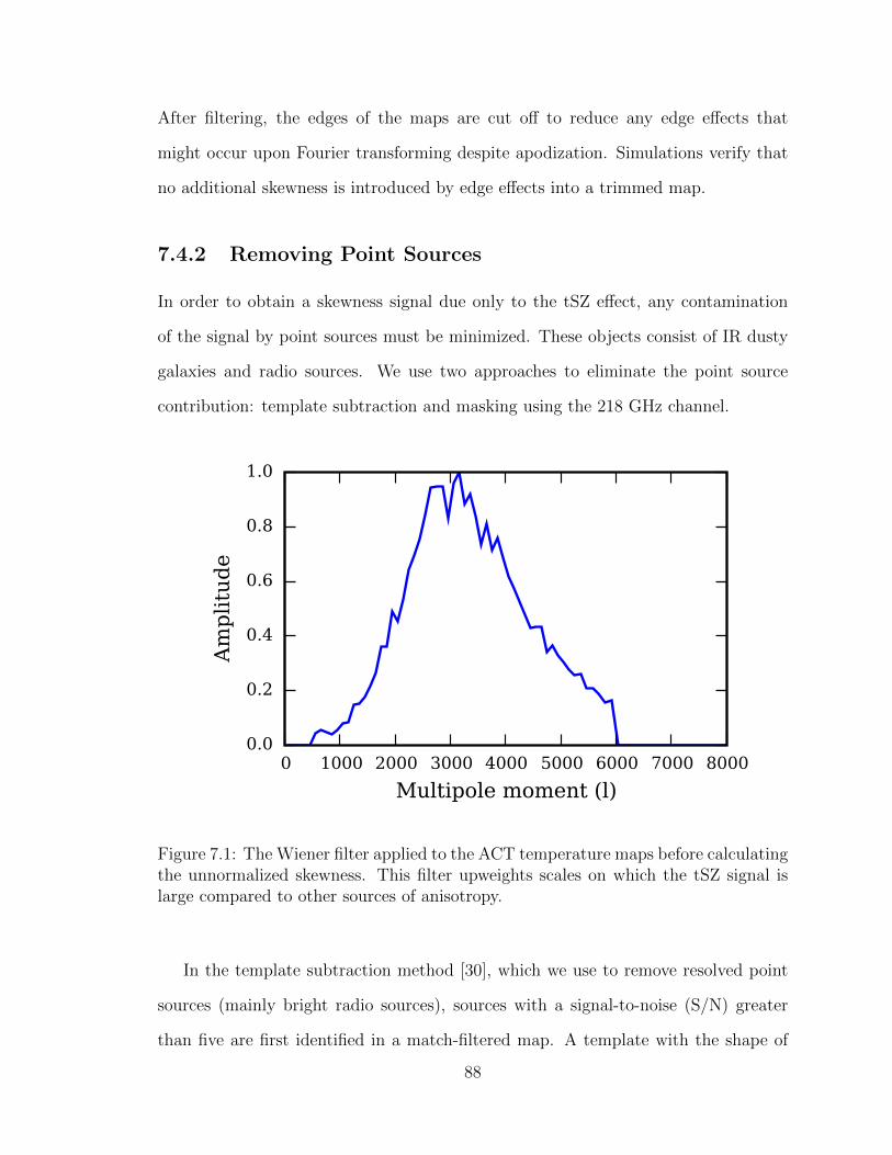
After filtering, the edges of the maps are cut off to reduce any edge effects that

might occur upon Fourier transforming despite apodization. Simulations verify that

no additional skewness is introduced by edge effects into a trimmed map.

7.4.2 Removing Point Sources

In order to obtain a skewness signal due only to the tSZ effect, any contamination

of the signal by point sources must be minimized. These objects consist of IR dusty

galaxies and radio sources. We use two approaches to eliminate the point source

contribution: template subtraction and masking using the 218 GHz channel.

0 1000 2000 3000 4000 5000 6000 7000 8000

Multipole moment (l)

0.0

0.2

0.4

0.6

0.8

1.0

Am

pli

tud

e

Figure 7.1: The Wiener filter applied to the ACT temperature maps before calculatingthe unnormalized skewness. This filter upweights scales on which the tSZ signal islarge compared to other sources of anisotropy.

In the template subtraction method [30], which we use to remove resolved point

sources (mainly bright radio sources), sources with a signal-to-noise (S/N) greater

than five are first identified in a match-filtered map. A template with the shape of

88

the ACT beam is then scaled to the appropriate peak brightness of each source, and

this profile is subtracted from the raw data. The process is iterated following the

CLEAN algorithm [31] until no more sources can be identified. We verify that this

procedure does not introduce skewness into the maps (e.g., through oversubtraction)

by checking that similar results are obtained using a different procedure for reducing

source contamination, in which we mask and in-paint pixels which contain bright

sources with S/N > 5 [32].

We take a second step to suppress the lower-flux, unresolved point sources (mainly

dusty galaxies) that remain undetected by the template subtraction algorithm. At

218 GHz, dusty galaxies are significantly brighter than at 148 GHz and the tSZ effect

is negligible. We construct a dusty galaxy mask by setting all pixels (which are

approximately 0.25 arcmin2) to zero that have a temperature in the 218 GHz maps

larger than a specified cutoff value. This cutoff is chosen to be 3.2 times the standard

deviation of the pixel values in the filtered 148 GHz map (3.2σ). This procedure

ensures regions with high flux from dusty galaxies are masked. We also set to zero

all pixels for which the temperature is lower than the negative of this cutoff, so that

the masking procedure does not introduce spurious skewness into the lensed CMB

distribution, which is assumed to have zero intrinsic skewness. The mask is then

applied to the 148 GHz map to reduce the point source contribution. Simulations

([33] for IR sources) verify that the masking procedure does not introduce spurious

skewness into the 148 GHz maps.

Finally, all pixels more than twelve standard deviations (12σ) from the mean are

also removed from the 148 GHz maps. Due to the ringing around very positive or

negative pixels caused by the Wiener filter, the surrounding eight arcminutes of these

points are also masked. This additional step slightly increases the S/N of the skewness

measurement by reducing the dependence on large outliers, enhances the information

content of low moments by truncating the tail of the pixel probability density function,

89

Figure 7.2: Histogram of the pixel temperature values in the filtered, masked ACTCMB temperature maps. A Gaussian curve is overlaid in red.

and ensures that any anomalous outlying points from possibly mis-subtracted bright

radio sources do not contribute to the skewness signal. Overall, 14.5% of the 148 GHz

map is removed by the masking procedure, though the removed points are random

with respect to the tSZ field and should not change the signal.

7.5 Results

7.5.1 Evaluating the Skewness

We compute the unnormalized skewness of the filtered and processed 148 GHz maps

by simply cubing and averaging the pixel values in real space. The result is⟨T 3⟩

=

−31 ± 6 µK3, a 5σ deviation from the null result expected for a signal without any

non-Gaussian components. The skewness of the CMB temperature distribution in our

filtered, processed maps is visible in the pixel value histogram shown in Fig. 2 (along

90

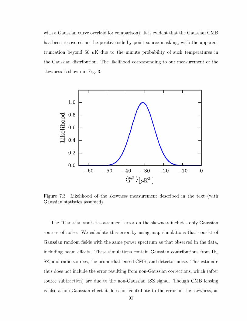
with a Gaussian curve overlaid for comparison). It is evident that the Gaussian CMB

has been recovered on the positive side by point source masking, with the apparent

truncation beyond 50 µK due to the minute probability of such temperatures in

the Gaussian distribution. The likelihood corresponding to our measurement of the

skewness is shown in Fig. 3.

60 50 40 30 20 10 0

T3

K3

0.0

0.2

0.4

0.6

0.8

1.0

Likelihood

Figure 7.3: Likelihood of the skewness measurement described in the text (withGaussian statistics assumed).

The “Gaussian statistics assumed” error on the skewness includes only Gaussian

sources of noise. We calculate this error by using map simulations that consist of

Gaussian random fields with the same power spectrum as that observed in the data,

including beam effects. These simulations contain Gaussian contributions from IR,

SZ, and radio sources, the primordial lensed CMB, and detector noise. This estimate

thus does not include the error resulting from non-Gaussian corrections, which (after

source subtraction) are due to the non-Gaussian tSZ signal. Though CMB lensing

is also a non-Gaussian effect it does not contribute to the error on the skewness, as

91

the connected part of the six-point function is zero to lowest order in the lensing

potential, and the connected part of the three-point function is also negligibly small

(see [34] and references therein).

We calculate errors that include non-Gaussian corrections by constructing more

realistic simulations. To construct such simulations, we add maps with simulated tSZ

signal from [35], which assume σ8 = 0.8, to realizations of a Gaussian random field

which has a spectrum such that the power spectrum of the combined map matches

that observed in the ACT temperature data. Given the simulated sky area, we obtain

39 statistically independent simulated maps, each of size 148 deg2. By applying an

identical procedure to the simulations as to the data, measuring the scatter amongst

the patches, and appropriately scaling the error to match the 237 deg2 of unmasked

sky in the processed map, we obtain a full error (including non-Gaussian corrections)

on the unnormalized skewness of 14 µK3. While this error is a robust estimate it

should be noted that the “error on the error” is not insignificant due to the moderate

simulated volume available. The scatter of skewness values measured from each of

the simulated maps is consistent with a Gaussian distribution. The estimate for the

full error is coincidentally the same as the standard error, 14 µK3, estimated from the

six patches into which the data are divided. The full error is used below in deriving

cosmological constraints from the skewness measurement.

7.5.2 The Origin of the Signal

Is the skewness dominated by massive clusters with large tSZ decrements – as sug-

gested by theoretical considerations described earlier – or by more numerous, less

massive clusters? To investigate this question, we mask clusters in our data which

were found in the 148 GHz maps using a matched filter as in [36]. All clusters de-

tected above a threshold significance value are masked; we vary this threshold and

measure the remaining skewness in order to determine the origin of the signal.

92

4 5 6 7 8 9 10

Minimum S/N of masked detected clusters

40

30

20

10

0

10

20

T3

K3

Figure 7.4: Plot of the skewness signal as a function of the minimum S/N of theclusters that are masked (this indicates how many known clusters are left in thedata, unmasked). The blue line is calculated using the full cluster candidate catalogobtained via matched filtering, while the green line uses a catalog containing onlyoptically-confirmed clusters [38]. Both lines have identical errors, but we only plotthem for the green line for clarity. Confirmed clusters source approximately two-thirds of the signal, which provides strong evidence that it is due to the tSZ effect.Note that one expects a positive bias of ≈ 4 µK3 for the S/N = 4 point of the blueline due to impurities in the full candidate catalog masking the tail of the Gaussiandistribution.

Fig. 4 shows a plot of the signal against the cluster detection significance cutoff.

We include calculations using both the full cluster candidate catalog obtained via

matched filtering as well a catalog containing only clusters confirmed optically using

the methodology of [37] on the SDSS Stripe 82 [38]. The SDSS Stripe 82 imaging data

cover ≈ 80% of the total map area, and thus some skewness signal will necessarily

arise from objects not accounted for in this catalog. The results for these two catalogs

agree when masking clusters with S/N ≥ 7, but differ slightly when masking lower

S/N clusters. This effect is likely due to the small shortfall in optical follow-up area

93

as well as a small number of false detections (i.e., impurity) in the candidate clusters

that have not yet been optically followed up.

Figure 7.5: A test for IR source contamination: similar to the blue line in Fig. 4, butwith a range of values of the cutoff used to construct an IR source mask in the 218GHz band. Any cutoff below ≈ 3.2σ gives similarly negative results and thus appearssufficient for point source removal, where σ = 10.3 µK is the standard deviation ofthe 148 GHz maps. For comparison, the standard deviation of the 218 GHz maps is≈ 2.2 times larger. The percentages of the map which are removed for the maskinglevels shown, from the least to the most strict cut, are 0.7, 2.5, 8.4, 14.5, 23.7, and36.6%.

Using either catalog, Fig. 4 implies that just under half of the tSZ skewness is

obtained from clusters that lie below a 5σ cluster detection significance, while the

remainder comes from the brightest and most massive clusters. The results of [36]

suggest that clusters detected at 5σ significance are roughly characterized by a mass

M500 = 5 × 1014M/h, where M500 is the mass enclosed within a radius such that

the mean enclosed density is 500 times the critical density at the cluster redshift.

This value corresponds to a virial mass of roughly M = 9 × 1014M/h, which was

94

also found to be the mass detection threshold for high-significance ACT clusters in

[37]. Fig. 4 thus demonstrates that roughly half of the tSZ skewness signal is due to

massive clusters with M & 1015M/h. The theoretical calculations described earlier

give similar results for the fraction of the signal coming from clusters above and

below this mass scale, which is significantly higher than the characteristic mass scale

responsible for the tSZ power spectrum signal.

Finally, the positive value in the full candidate catalog line shown in Fig. 4 when

masking clusters above S/N = 4 is consistent with zero. When masking at this level

(with the candidate catalog which contains some impurities), we slightly cut into the

negative pixel values in the Gaussian component of Fig. 2, leading to a small spurious

positive skewness. For the points we plot, we calculate that this bias is only non-

negligible for the S/N = 4 cut, where it is ≈ 4 µK3. This bias effectively explains the

small positive offset seen in Fig. 4. However, we discuss positive skewness due to any

possible residual point source contamination below. Overall, the dependence of the

measured skewness on cluster masking shown in Fig. 4 provides strong evidence that

it is caused by the tSZ effect.

7.5.3 Testing for Systematic Infrared Source Contamination

Despite our efforts to remove point sources, a small residual point source contami-

nation of the signal could remain, leading to an underestimate of the amplitude of

the tSZ skewness. To investigate this systematic error source, we vary the level at

which point sources are masked in the 218 GHz maps (the original level is 3.2 times

the standard deviation of the pixel values in the filtered 148 GHz map (3.2σ), as

described above). The results of this test are shown in Fig. 5, which uses the full

catalog of cluster candidates as described in Fig. 4, since the optically-confirmed cat-

alog does not yet cover the entire ACT map. Note that masking at 3.2σ results in

a skewness measurement which agrees with its apparent asymptotic limit as the IR

95

contamination is reduced, within the expected fluctuations due to masking. While

a slightly more negative skewness value can be measured for some masking levels

stricter than the 3.2σ level chosen in the analysis, fluctuations upon changing the

unmasked area of the sky are expected, so that it can not be rigorously inferred that

IR contamination is reduced between 3.2σ and 2.65σ. Fig. 5 suggests that masking

at the 3.2σ level sufficiently removes any contamination by IR sources, and stricter

cuts will reduce the map area and increase statistical errors unnecessarily.

However, to further estimate the residual point source contamination in the 148

GHz maps, we process simulations of IR sources from [33] (with source amplitudes

scaled down by 1.7 to match recent observations, as in [39]) with the same masking

procedure as that applied to the data (described in §7.4.2), creating a mask in a

simulated 218 GHz map, and applying it to a simulated IR source signal at 148 GHz.

We find a residual signal of⟨T 3⟩

= 3.9 ± 0.1 µK3. We treat this result as a bias in

deriving cosmological constraints from the tSZ skewness in the following section.

We also investigate a linear combination of the 148 and 218 GHz maps that

should have minimal IR source levels, namely, an appropriately scaled 218 GHz map

subtracted from a 148 GHz map. Assuming that the spatial distribution of the point

sources is not affected by the difference in observation frequency between 148 and

218 GHz and a single spectral index can be applied to all sources, a simple factor of

≈ 3.2 [13] relates a point source’s signal in the two different frequency bands. We

find that the appropriate linear combination (subtracting 1/3.2 times the 220 GHz

map from the 148 GHz map) produces a signal in agreement with that resulting from

the previously described masking procedure, although the additional noise present in

the 218 GHz maps slightly reduces the significance of the detection.

96

7.6 Cosmological Interpretation

To obtain cosmological information from the measured amplitude of the unnormalized

skewness, we compare our results with two different sets of tSZ simulations [33, 35].

Both sets of simulations are run with σ8 = 0.8, but differ in their treatment of

the ICM. The simulation of [35] is a fully hydrodynamic cosmological simulation that

includes sub-grid prescriptions for feedback from active galactic nuclei, star formation,

and radiative cooling. The simulation also captures non-thermal pressure support due

to turbulence and other effects, which significantly alters the ICM pressure profile.

The simulation of [33] is a large dark matter-only N -body simulation that is post-

processed to include gas according to a polytropic prescription. This simulation also

accounts for non-thermal pressure support (though with a smaller amount than [35]),

and matches the low-redshift X-ray data presented in [17].

We perform the same filtering and masking as that applied to the data in order

to analyze the simulation maps. For both simulations, the filtering reduces the signal

by ≈ 95% compared to the unfiltered value. For the simulations of [35], we measure⟨T 3⟩S

= −37 µK3, with negligible errors (the superscript S indicates a simulated

value). However, this value is complicated by the fact that these simulations only

include halos below z = 1. An analytic estimate for the skewness contribution due to

halos with z > 1 from Eq. (7.1) gives a 6% correction, which yields⟨T 3⟩S

= −39 µK3.

For the simulations of [33], we measure⟨T 3⟩S

= −50 µK3, with errors also negligible

for the purposes of cosmological constraints.

We combine these simulation results with our calculated scalings of the skewness

and the sixth moment with σ8 to construct a likelihood:

L(σ8) = exp

−(⟨T 3⟩D − ⟨T 3

⟩th(σ8)

)2

2σ2th(σ8)

(7.3)

97

where⟨T 3⟩D

is our measured skewness value and the theoretically expected skewness

as a function of σ8 is given by

⟨T 3⟩th

(σ8) =⟨T 3⟩S ( σ8

0.8

)α3

. (7.4)

The likelihood in Eq. (7.3) explicitly accounts for the fact that σ2th, the variance

of the skewness, depends on σ8 — a larger value of σ8 leads to a larger expected

variance in the tSZ skewness signal. In particular, the variance of the tSZ skewness is

described by a sixth moment, so it scales as σα68 . As determined above, the Gaussian

and non-Gaussian errors on the skewness are 6 µK3 and√

142 − 62 µK3 = 12.6 µK3,

respectively. We approximate the dependence of the full error on σ8 by assuming that

only the non-Gaussian component scales with σ8; while this is not exact, as some of

the Gaussian error should also scale with σ8, small differences in the size or scaling

of the Gaussian error component cause negligible changes in our constraints on σ8.

Finally, although we have argued previously that IR source contamination is es-

sentially negligible, we explicitly correct for the residual bias as calculated in the

previous section. Thus, we replace⟨T 3⟩D

= −31 µK3 with⟨T 3⟩Dcorr

= −31− 3.9 µK3

in Eq. (7.3). (Note that this bias correction only shifts the central value derived for

σ8 below by roughly one-fifth of the 1σ confidence interval.) Moreover, in order to

be as conservative as possible, we also model the effect of residual point sources by

including an additional IR contamination error (with the same value as the residual

IR source contamination, 3.9 µK3) in our expression for the variance of the skewness:

σ2th(σ8) = 62 µK6 + 12.62

( σ8

0.8

)α6

µK6 + 3.92 µK6. (7.5)

Using the likelihood in Eq. (7.3), we obtain confidence intervals and derive a

constraint on σ8. Our likelihood and hence our constraints depend in principle on

which simulation we use to calculate⟨T 3⟩S

, as well as on the values we choose for

98

α3 and α6. Using the simulations of [35] and the scalings determined above for the

profile from [16], we find σ8 = 0.79+0.03−0.03 (68% C.L.) +0.06

−0.06 (95% C.L.). In Table I,

we compare the constraints on σ8 obtained from the use of different scalings and

simulated skewness values; the constraints are insensitive to both the pressure profile

used to derive the scaling laws and the choice of simulation used to compute the

skewness.

For comparison, the final release from the Chandra Cluster Cosmology Project

found σ8 = 0.803±0.0105, assuming Ωm = 0.25 (there is a strong degeneracy between

σ8 and Ωm for X-ray cluster measurements that probe the mass function) [40]. Perhaps

more directly comparable, recent studies of the tSZ power spectrum have found σ8 =

0.77 ± 0.04 (statistical error only) [13] and σ8 = 0.807 ± 0.016 (statistical error and

approximately estimated systematic error due to theoretical uncertainty) [41]. Our

results are also comparable to recent constraints using number counts of SZ-detected

clusters from ACT and SPT, which found σ8 = 0.851 ± 0.115 (fully marginalizing

over uncertainties in the mass-SZ flux scaling relation) [42] and σ8 = 0.807 ± 0.027

(marginalizing over uncertainties in an X-ray-based mass-SZ flux scaling relation) [43],

respectively. Although more than half of the tSZ skewness signal that we measure

is sourced by detected clusters (i.e., the same objects used in the number counts

analyses), our method also utilizes cosmological information from clusters that lie

below the individual detection threshold, which gives it additional statistical power.

Finally, note that we have fixed all other cosmological parameters in this analysis, as

σ8 is by far the dominant parameter for the tSZ skewness [44]. However, marginalizing

over other parameters will slightly increase our errors.

To evaluate the theoretical systematic uncertainty in the amplitude of the filtered

skewness due to unknown ICM astrophysics, we test the effect of different gas pre-

scriptions by analyzing simulations from [35] with all forms of feedback, radiative

cooling and star formation switched off, leading to an adiabatic ICM gas model. For

99

these adiabatic simulations we find⟨T 3⟩S

= −56 µK3 (after applying the 6% cor-

rection mentioned earlier), which for the skewness we measure in our data would

imply σ8 = 0.77+0.02−0.02 (68% C.L.)+0.05

−0.05 (95% C.L.). Turning off feedback and all sub-

grid physics is a rather extreme case, so the systematic theoretical uncertainty for a

Battaglia⟨T 3⟩S

Sehgal⟨T 3⟩S

Battaglia α3, α6 0.79+0.03−0.03

+0.06−0.06 0.77+0.03

−0.02+0.05−0.05

Arnaud α3, α6 0.79+0.03−0.03

+0.06−0.06 0.77+0.02

−0.02+0.05−0.05

K-S α3, α6 0.79+0.03−0.03

+0.07−0.06 0.77+0.03

−0.03+0.06−0.05

Table 7.1: Constraints on σ8 derived from our skewness measurement using twodifferent simulations and three different scalings of the skewness and its variancewith σ8. The top row lists the simulations used to calculate the expected skewnessfor σ8 = 0.8 [35, 33]; the left column lists the pressure profiles used to calculate thescaling of the skewness and its variance with σ8 [16, 17, 25]. The errors on σ8 shownare the 68% and 95% confidence levels.

typical simulation with some form of feedback should be slightly smaller than the sta-

tistical error from the measurement, though still non-negligible. This contrasts with

measurements of σ8 via the tSZ power spectrum, for which the theoretical system-

atic uncertainty is comparable to or greater than the statistical uncertainty [13, 41].

As highlighted earlier, this difference can be traced to the dependence of the power

spectrum amplitude on the ICM astrophysics within low-mass, high-redshift clus-

ters. The skewness, on the other hand, is dominated by more massive, lower-redshift

clusters that are less affected by uncertain non-gravitational feedback mechanisms

and are more precisely constrained by observations. Nonetheless, as the statistical

uncertainty decreases on future measurements of the tSZ skewness, the theoretical

systematic error will quickly become comparable, and thus additional study of the

ICM electron pressure profile will be very useful.

100

7.7 Conclusions

As the thermal Sunyaev-Zel’dovich field is highly non-Gaussian, measurements of

non-Gaussian signatures such as the skewness can provide cosmological constraints

that are competitive with power spectrum measurements. We have presented a first

measurement of the unnormalized skewness⟨T 3(n)

⟩in ACT CMB maps filtered for

high signal to noise. As this is a purely non-Gaussian signature, primordial CMB

and instrumental noise cannot be confused with or bias the signal, unlike measure-

ments of the tSZ power spectrum. We measure the skewness at 5σ significance:⟨T 3(n)

⟩= −31± 6 µK3 (Gaussian statistics assumed). Including non-Gaussian cor-

rections increases the error to ± 14 µK3. Using analytic calculations and simulations

to translate this measurement into constraints on cosmological parameters, we find

σ8 = 0.79+0.03−0.03 (68% C.L.) +0.06

−0.06 (95% C.L.), with a slightly smaller but non-negligible

systematic error due to theoretical uncertainty in the ICM astrophysics. This de-

tection represents the first realization of a new, independent method to measure σ8

based on the tSZ skewness, which has different systematic errors than several other

common methods. With larger maps and lower noise, tSZ skewness measurements

promise significantly tighter cosmological constraints in the near future.

7.8 Acknowledgements

As this manuscript was being prepared, we learned of related theoretical work by the

authors of [44], and we acknowledge very helpful discussions with the members of

this collaboration. This work was supported by the U.S. NSF through awards AST-

0408698, PHY-0355328, AST-0707731 and PIRE-0507768, as well as by Princeton

Univ., the Univ. of Pennsylvania, FONDAP, Basal, Centre AIUC, RCUK Fellow-

ship (JD), NASA grant NNX08AH30G (SD, AH, TM), NSERC PGSD (ADH), NSF

AST-0546035 and AST-0807790 (AK), NSF PFC grant PHY-0114422 (ES), KICP Fel-

101

lowship (ES), SLAC no. DE-AC3-76SF00515 (NS), ERC grant 259505 (JD), BCCP

(SD), and the NSF GRFP (BDS, BLS). We thank B. Berger, R. Escribano, T. Evans,

D. Faber, P. Gallardo, A. Gomez, M. Gordon, D. Holtz, M. McLaren, W. Page, R.

Plimpton, D. Sanchez, O. Stryzak, M. Uehara, and Astro-Norte for assistance with

ACT. ACT operates in the Parque Astronomico Atacama in northern Chile under

the auspices of Programa de Astronomıa, a program of the Comision Nacional de

Investigacion Cientıfica y Tecnologica de Chile (CONICYT).

102

References

[1] Fowler, J. W., Niemack, M. D., Dicker, S. R., et al. 2007, Applied Optics, 46,

3444

[2] Dunner, R., Hasselfield, M., Marriage, T. M., et al. in prep.

[3] Swetz, D. S., Ade, P. A. R., Amiri, M., et al. 2011, ApJS, 194, 41

[4] Carlstrom, J. E., Ade, P. A. R., Aird, K. A., et al. 2011, PASP, 123, 568

[5] Schaffer, K. K., Crawford, T. M., Aird, K. A., et al. 2011, ApJ, 743, 90

[6] Zel’dovich, Y. B., & Sunyaev, R. A. 1969, Ap&SS, 4, 301

[7] Sunyaev, R. A., & Zel’dovich, Y. B. 1970, Ap&SS, 7, 3

[8] Staniszewski, Z., Ade, P. A. R., Aird, K. A., et al. 2009, ApJ, 701, 32

[9] Vanderlinde, K., Crawford, T. M., de Haan, T., et al. 2010, ApJ, 722, 1180

[10] Hincks, A. D., Acquaviva, V., Ade, P. A. R., et al. 2010, ApJS, 191, 423

[11] Marriage, T. A., Acquaviva, V., Ade, P. A. R., et al. 2011, ApJ, 737, 61

[12] Sehgal, N., Trac, H., Acquaviva, V., et al. 2011, ApJ, 732, 44

[13] Dunkley, J., Hlozek, R., Sievers, J., et al. 2011, ApJ, 739, 52

[14] Keisler, R., Reichardt, C. L., Aird, K. A., et al. 2011, ApJ, 743, 28

103

[15] Rubino-Martın, J. A., & Sunyaev, R. A. 2003, Mon. Not. R. Astron. Soc, 344,

1155

[16] Battaglia, N., Bond, J. R., Pfrommer, C., & Sievers, J. L. 2011, arXiv:1109.3711

[17] Arnaud, M., Pratt, G. W., Piffaretti, R., et al. 2010, A&A, 517, A92

[18] Shaw, L. D., Nagai, D., Bhattacharya, S., & Lau, E. T. 2010, ApJ, 725, 1452

[19] Battaglia, N., Bond, J. R., Pfrommer, C., & Sievers, J. L. 2011, arXiv:1109.3709

[20] Hajian, A., Viero, M. P., Addison, G., et al. 2012, ApJ, 744, 40

[21] Komatsu, E., Dunkley, J., Nolta, M. R., et al. 2009, ApJS, 180, 330

[22] Komatsu, E., & Kitayama, T. 1999, ApJ, 526, L1

[23] Tinker, J., Kravtsov, A. V., Klypin, A., et al. 2008, ApJ, 688, 709

[24] Sheth, R. K., & Tormen, G. 2002, Mon. Not. R. Astron. Soc, 329, 61

[25] Komatsu, E., & Seljak, U. 2002, Mon. Not. R. Astron. Soc, 336, 1256

[26] Hill, J. C., & Sherwin, B. D. 2012, arXiv:1205.5794

[27] Trac, H., Bode, P., & Ostriker, J. P. 2011, ApJ, 727, 94

[28] Holder, G. P., McCarthy, I. G., & Babul, A. 2007, Mon. Not. R. Astron. Soc,

382, 1697

[29] Hajian, A., Acquaviva, V., Ade, P. A. R., et al. 2011, ApJ, 740, 86

[30] Marriage, T. A., Baptiste Juin, J., Lin, Y.-T., et al. 2011, ApJ, 731, 100

[31] Hogbom, J. A. 1974, A&AS, 15, 417

[32] Bucher, M., & Louis, T. 2011, arXiv:1109.0286

104

[33] Sehgal, N., Bode, P., Das, S., et al. 2010, ApJ, 709, 920

[34] Lewis, A., & Challinor, A. 2006, Physics Reports, 429, 1

[35] Battaglia, N., Bond, J. R., Pfrommer, C., Sievers, J. L., & Sijacki, D. 2010, ApJ,

725, 91

[36] Marriage, T. A., Acquaviva, V., Ade, P. A. R., et al. 2011, ApJ, 737, 61

[37] Menanteau, F., Gonzalez, J., Juin, J.-B., et al. 2010, ApJ, 723, 1523

[38] Menanteau, F., et al. in prep.

[39] van Engelen, A., Keisler, R., Zahn, O., et al. 2012, arXiv:1202.0546

[40] Vikhlinin, A., Kravtsov, A. V., Burenin, R. A., et al. 2009, ApJ, 692, 1060

[41] Reichardt, C. L., Shaw, L., Zahn, O., et al. 2011, arXiv:1111.0932

[42] Sehgal, N., Trac, H., Acquaviva, V., et al. 2011, ApJ, 732, 44

[43] Reichardt, C. L., Stalder, B., Bleem, L. E., et al. 2012, arXiv:1203.5775

[44] Bhattacharya, S., Nagai, D., Shaw, L., Crawford, T., & Holder, G. P. 2012,

arXiv:1203.6368

105

Appendix A

Lensing Simulation and Power

Spectrum Estimation for High

Resolution CMB Polarization

Maps

A.1 Abstract

We present efficient algorithms for CMB lensing simulation and power spectrum es-

timation for flat-sky CMB polarization maps. We build a pure B-mode estimator to

remedy E to B leakage due to partial sky coverage. We show that our estimators are

unbiased, and consistent with the projected errors. We demonstrate our algorithm

using simulated observations of small sky patches with realistic noise and weights for

upcoming CMB polarization experiments.

106

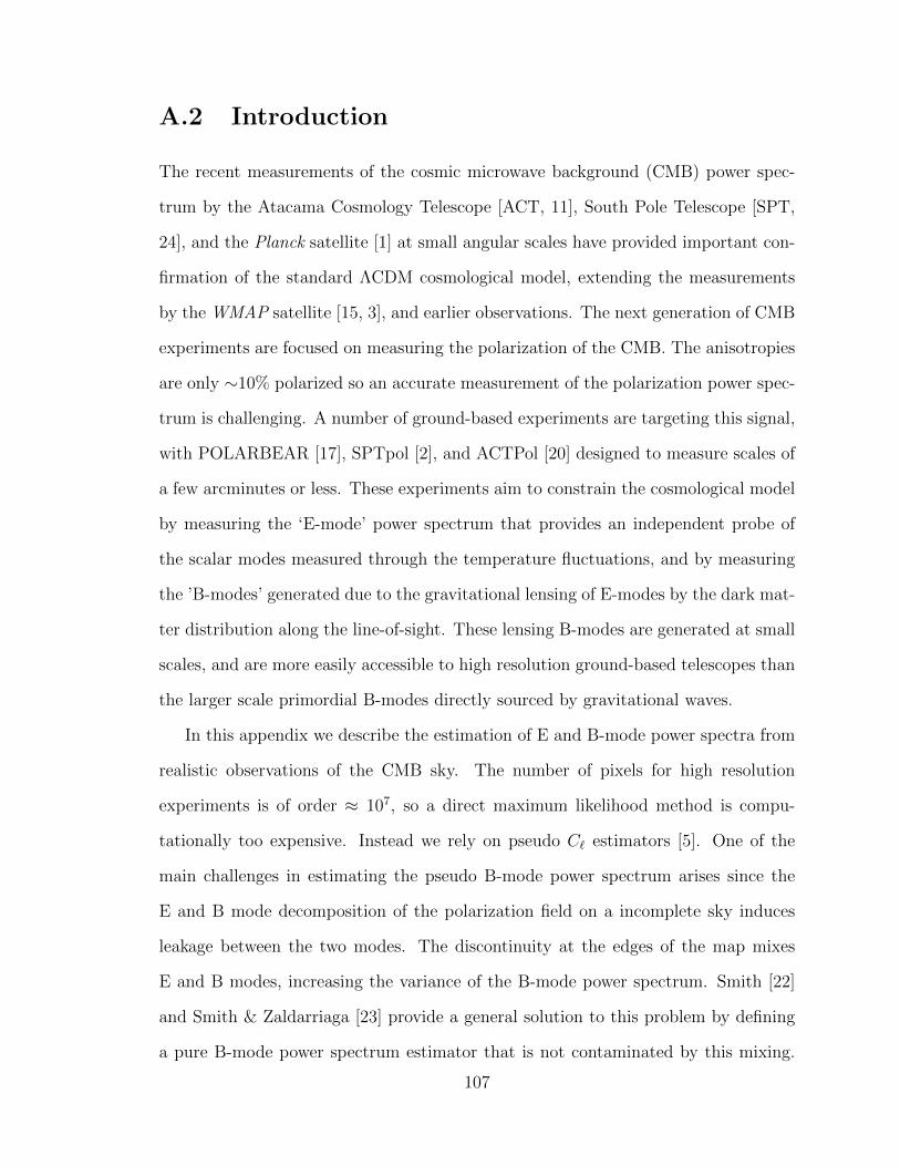
A.2 Introduction

The recent measurements of the cosmic microwave background (CMB) power spec-

trum by the Atacama Cosmology Telescope [ACT, 11], South Pole Telescope [SPT,

24], and the Planck satellite [1] at small angular scales have provided important con-

firmation of the standard ΛCDM cosmological model, extending the measurements

by the WMAP satellite [15, 3], and earlier observations. The next generation of CMB

experiments are focused on measuring the polarization of the CMB. The anisotropies

are only ∼10% polarized so an accurate measurement of the polarization power spec-

trum is challenging. A number of ground-based experiments are targeting this signal,

with POLARBEAR [17], SPTpol [2], and ACTPol [20] designed to measure scales of

a few arcminutes or less. These experiments aim to constrain the cosmological model

by measuring the ‘E-mode’ power spectrum that provides an independent probe of

the scalar modes measured through the temperature fluctuations, and by measuring

the ’B-modes’ generated due to the gravitational lensing of E-modes by the dark mat-

ter distribution along the line-of-sight. These lensing B-modes are generated at small

scales, and are more easily accessible to high resolution ground-based telescopes than

the larger scale primordial B-modes directly sourced by gravitational waves.

In this appendix we describe the estimation of E and B-mode power spectra from

realistic observations of the CMB sky. The number of pixels for high resolution

experiments is of order ≈ 107, so a direct maximum likelihood method is compu-

tationally too expensive. Instead we rely on pseudo C` estimators [5]. One of the

main challenges in estimating the pseudo B-mode power spectrum arises since the

E and B mode decomposition of the polarization field on a incomplete sky induces

leakage between the two modes. The discontinuity at the edges of the map mixes

E and B modes, increasing the variance of the B-mode power spectrum. Smith [22]

and Smith & Zaldarriaga [23] provide a general solution to this problem by defining

a pure B-mode power spectrum estimator that is not contaminated by this mixing.

107

In Section 2, we adapt their algorithm for flat sky maps, and demonstrate that the

algebra simplifies considerably under the flat-sky approximation.

In Section 3, we introduce a novel technique for generating high resolution lensed

CMB maps. Different methods have been proposed to do this, often using a remap-

ping between pixels [18] and an interpolation scheme. We present a hybrid method

that combines pixel remapping and a Taylor series decomposition of the lensed field.

In Section 4, we use simulated observations from the ACTPol experiment to generate

non-uniform realizations of the experimental noise. We then test our lensing simula-

tion and power spectrum estimation method, and its optimality, using Monte Carlo

simulations.

A.3 E/B leakage in the flat sky approximation

In this section we review the issue of leakage of power between polarization types due

to incomplete sky coverage. This issue has been discussed in previous studies targeting

observations over large areas [e.g., 19, 22, 23, 13, 9, 25, 8, 7, 14]. We demonstrate how

the ‘pure’ estimators of the different polarization types can be applied in the flat-sky

approximation, relevant to small patches of the sky.

A.3.1 Notation

For linear polarization, the Stokes parameter Q quantifies the polarization in the

x-y direction and U quantifies it along axes rotated by 45. Following e.g., [6], the

polarization tensor is given by

Pab(~x) =1

2

Q(~x) U(~x)

U(~x) −Q(~x)

. (A.1)

108

Any 2× 2 symmetric traceless tensor can be uniquely decomposed into two parts of

the form EabA = (−∂a∂b + 12δab∇2)A and BabB = 1

2(εac∂

c∂b + εbc∂c∂a)B where A and

B are scalar functions [e.g., 16]. The Fourier modes ei~~x provide a basis for a scalar

function in the plane, so one can define

(Eei~.~x)ab = N~Eab(ei

~~x) = N~

(`a`b −

~2

2δab

)ei~~x

(Bei~.~x)ab = M~Bab(ei

~~x) = −M~

2(εac`

c`b + εbc`c`a) e

i~~x, (A.2)

where N and M are normalization coefficients that satisfy the orthogonality relation

∫d2x(Eei

~~x)∗ab(Eei

~′~x)ab = δ(~− ~′), (A.3)

and similarly for Bei~~x. Expanding the polarization field in this basis, it can be

expressed as a combination of parity even (E) and odd (B) modes

Pab(~x) =1√2

∫d~E(~)(Eei

~~x)ab +B(~)(Bei~~x)ab,

E(~) =2

`2

∫d2xPab(~x)Eab(e−i~~x),

B(~) =2

`2

∫d2xPab(~x)Bab(e−i~~x). (A.4)

This is equivalent to the spin formalism introduced by Seljak & Zaldarriaga [21].

Defining φ` as the angle between the vector ~ and the `x axis, E and B take the

simple form

E(~) = Q(~) cos 2φ` + U(~) sin 2φ`,

B(~) = −Q(~) sin 2φ` + U(~) cos 2φ` (A.5)

or equivalently E(~)± iB(~) = e∓2iφ`(Q(~)± iU(~)).

109

A.3.2 Partial sky coverage

Observations with modern high resolution experiments are typically performed on a

small fraction of the sky, of area Ω [e.g., 24, 11]. The observed region can be described

by a window function

W (~x) =

w(~x) if ~x ∈ Ω

0 otherwise(A.6)

which modifies the observed Q and U components such that Q(~x) = W (~x)Q(~x) and

U(~x) = W (~x)U(~x). Propagating the effects of the window function into the E and B

modes calculated as in Eqn. A.5, the window functions mix E and B modes to give

the modified modes

E(~) =

∫d~′W (~− ~′)[E(~′) cos 2(φ`′ − φ`)−B(~′) sin 2(φ`′ − φ`)],

B(~) =

∫d~′W (~− ~′)[E(~′) sin 2(φ`′ − φ`) +B(~′) cos 2(φ`′ − φ`)]. (A.7)

The power spectra of these modified modes are then

〈E(~)E∗(~)〉 =

∫d~′|W (~− ~′)|2[CEE(`′) cos2 2(φ`′ − φ`) + CBB(`′) sin2 2(φ`′ − φ`)],

〈B(~)B∗(~)〉 =

∫d~′|W (~− ~′)|2[CEE(`′) sin2 2(φ`′ − φ`) + CBB(`′) cos2 2(φ`′ − φ`)].

(A.8)

Since CEE is expected to be an order of magnitude larger than CBB, this mixing

therefore leads to significant contamination of the B-modes by the leaked-in E-modes.

This is illustrated in Figure A.1, which also highlights that the leakage is localized

close to the edges of the map, or to the edges of holes due to masking of bright point

110

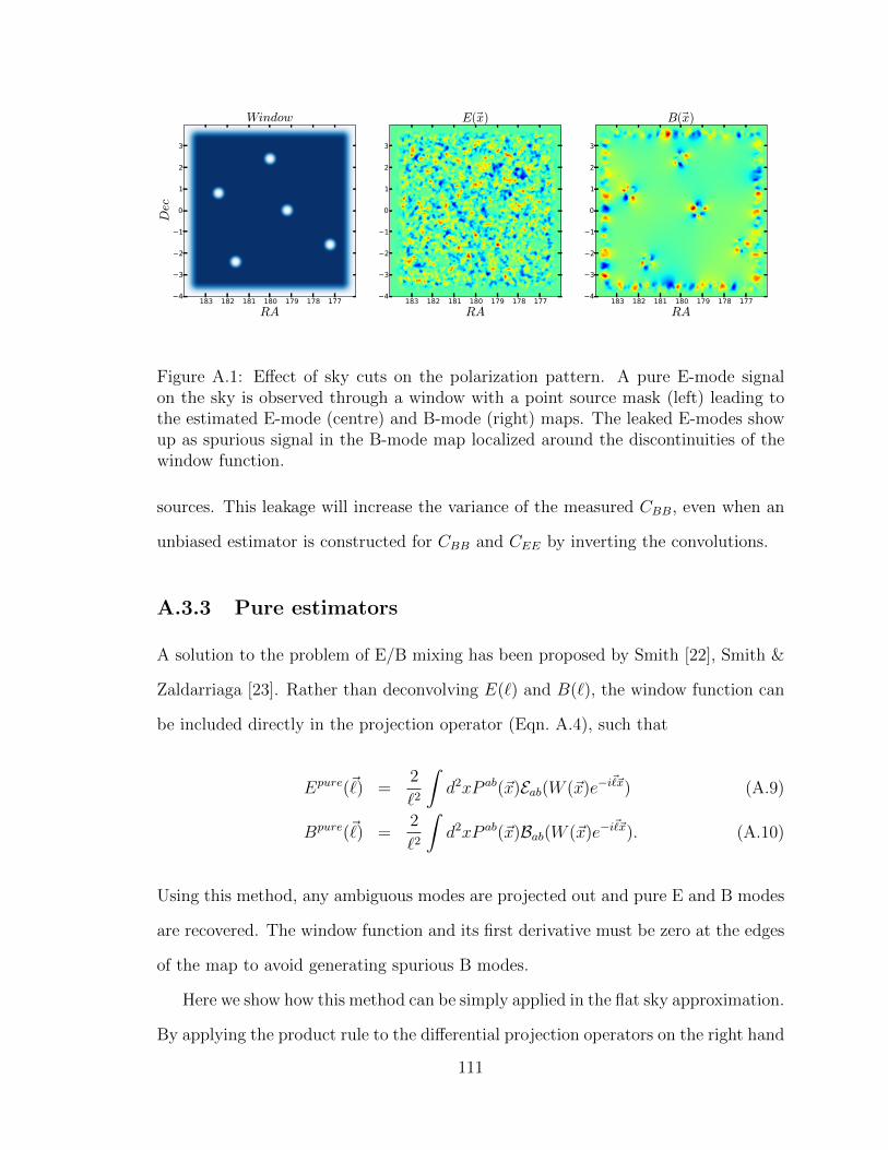
Figure A.1: Effect of sky cuts on the polarization pattern. A pure E-mode signalon the sky is observed through a window with a point source mask (left) leading tothe estimated E-mode (centre) and B-mode (right) maps. The leaked E-modes showup as spurious signal in the B-mode map localized around the discontinuities of thewindow function.

sources. This leakage will increase the variance of the measured CBB, even when an

unbiased estimator is constructed for CBB and CEE by inverting the convolutions.

A.3.3 Pure estimators

A solution to the problem of E/B mixing has been proposed by Smith [22], Smith &

Zaldarriaga [23]. Rather than deconvolving E(`) and B(`), the window function can

be included directly in the projection operator (Eqn. A.4), such that

Epure(~) =2

`2

∫d2xP ab(~x)Eab(W (~x)e−i

~~x) (A.9)

Bpure(~) =2

`2

∫d2xP ab(~x)Bab(W (~x)e−i

~~x). (A.10)

Using this method, any ambiguous modes are projected out and pure E and B modes

are recovered. The window function and its first derivative must be zero at the edges

of the map to avoid generating spurious B modes.

Here we show how this method can be simply applied in the flat sky approximation.

By applying the product rule to the differential projection operators on the right hand

111

sides of the above equations, we obtain expressions for the pure E and B modes. The

Bpure(~) mode is given by

Bpure(~) =2

`2

∫d2xW (~x)P ab(~x)Bab(e−i

~~x) +1

`2

∫d2x

[2Q∂x∂yW + U(∂2

y − ∂2x)W

]e−i

~~x

− 2i

`

∫d2x [Q(~x)(∂yW cosφ` + ∂xW sinφ`) + U(~x)(∂yW sinφ` − ∂xW cosφ`)] e

−i~~x.

(A.11)

The first term is the standard “naive” B mode estimator and the second and third

terms cancel the window-induced leakage from E to B modes, involving derivatives of

the window function. This expression is convenient for numerical uses as it does not

require the calculation of derivatives of noisy data. The pure estimator removes the

E/B leakage, but the remaining mode coupling effect induced by applying a window

to the observed sky still needs to be deconvolved.

To work out this effect, we can simplify the algebra if we express the pure estimator

in term of the χ variables [e.g., 19], with

χE(~x) = −1

2

[ðð(Q+ iU)(~x) + ðð(Q− iU)(~x)

],

χB(~x) =i

2

[ðð(Q+ iU)(~x)− ðð(Q− iU)(~x)

], (A.12)

where the spin raising and spin lowering operators are defined as ð = −(∂x + i∂y),

and ð = −(∂x− i∂y). After some algebra we find simple expressions for the two pure

modes,1

Bpure(~) =1

`2

∫d~xχB(~x)W (~x)e−i

~~x,

Epure(~) =1

`2

∫d~xχE(~x)W (~x)e−i

~~x. (A.13)

1This is most directly verified by inserting the definition of χB/E into the above integrals andintegrating by parts twice; the result obtained is identical to the original form of the pure estimators.

112

The simple expressions for the pure estimators using the χ variables are convenient

for computing this mode-to-mode coupling. Noting that

χE(~x) =

∫d~E(~)`2ei

~~x,

χB(~x) =

∫d~B(~)`2ei

~~x, (A.14)

we find that the coupling between modes is

〈Bpure(~)B∗pure(~)〉 =1

`4

⟨∫d~xχB(~x)W (~x)e−i

~~x

∫d~x′χB(~x′)W (~x′)ei

~~x′⟩,

=1

`4

∫d~′|W (~− ~′)|2`′4CBB(~′) (A.15)

for the B-modes, and

〈Epure(~)E∗pure(~)〉 =1

`4

∫d~′|W (~− ~′)|2`′4CEE(~′) (A.16)

for the E-modes. Here we have used 〈χB(~′)χ∗B(~′′)〉 = δ(~′− ~′′)`′4CBB(~′). In practice

using the pure E mode power spectrum estimator is unnecessary since the B-to-E

leakage is small so the advantage of using a pure estimator is lost and results in a

loss of sensitivity. We choose to use a hybrid approach [14], where the B mode power

spectrum is computed using the pure formalism (Eqn. A.11) and the E modes power

spectrum is computed via the standard pseudo power spectrum formalism.

A.4 Generating gravitationally lensed simulations

On their way from the surface of last scattering, the photons are deflected by the

gravitational field of the intervening large scale structure. Accurate lensing simula-

tions are essential for recovering the statistical property of the observed CMB. In the

weak field limit, the lensing results in a simple remapping of the temperature by a

113

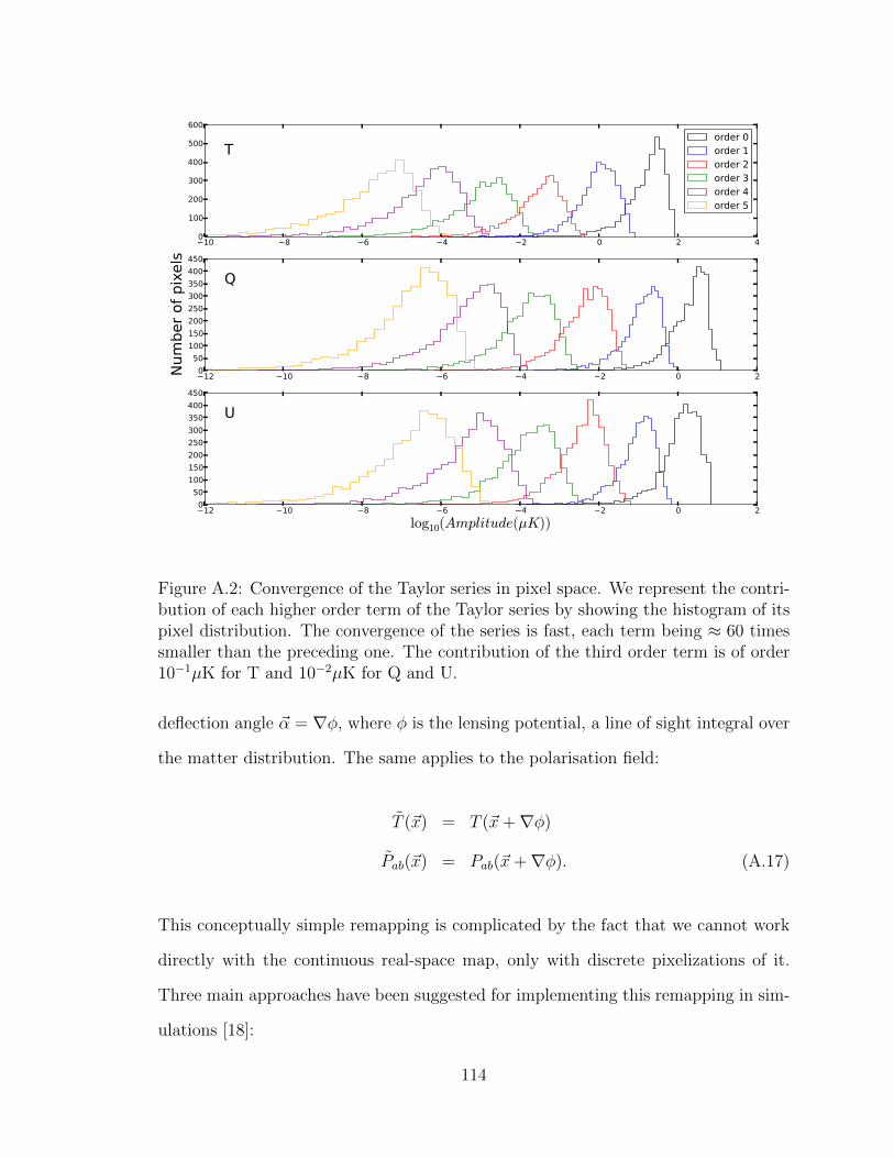
Figure A.2: Convergence of the Taylor series in pixel space. We represent the contri-bution of each higher order term of the Taylor series by showing the histogram of itspixel distribution. The convergence of the series is fast, each term being ≈ 60 timessmaller than the preceding one. The contribution of the third order term is of order10−1µK for T and 10−2µK for Q and U.

deflection angle ~α = ∇φ, where φ is the lensing potential, a line of sight integral over

the matter distribution. The same applies to the polarisation field:

T (~x) = T (~x+∇φ)

Pab(~x) = Pab(~x+∇φ). (A.17)

This conceptually simple remapping is complicated by the fact that we cannot work

directly with the continuous real-space map, only with discrete pixelizations of it.

Three main approaches have been suggested for implementing this remapping in sim-

ulations [18]:

114

1. Go directly from frequency domain to the lensed positions, i.e. T (~x+

~α) =∑

~F−1~ (~x+ ~α)T~, where F−1

~ (~x) is the inverse Fourier transform operator,

and T~ are the harmonic coefficients of the unlensed map. This approach is

exact, but computationally inefficient because the shifted positions will not in

general form a regular grid, and one hence cannot use Fast Fourier Transforms

(FFT).

2. Taylor expand the field: This is straightforward, but has been found to

converge slowly at small scales.

3. Pixel remapping: Truncate the displacement to the nearest pixel, and read

off the corresponding pixel value. This remapping must be done at much higher

resolution than the physical scales of interest in the map in order to avoid

pixelization errors, and hence comes at a large cost both in terms of CPU-time

and memory. It is therefore sometimes combined with pixel-space interpolation

schemes.

We present a simple modification to the Taylor expansion method that addresses its

slow convergence. In general, the Taylor expansion of a function f(x) around a point

x0 becomes less accurate as the distance from x0 grows, and conversely, the expansion

can be truncated earlier if one can expand around a point close to where one wishes

to evaluate the function. The Taylor remapping method above expands T (~x + ~α)

around the point ~α = 0, and the reason for the slow convergence is that ~α can be

relatively large. A better choice is to expand around the pixel center ~α0 closest to ~α,

which is already exactly available, resulting in the following expansion

T (~x) = T (~x+ ~α0 + ~∆α) = T (~x+ ~α0) + ∆αc[∂cT ](~x+ ~α0)

+1

2∆αc∆αd[∂c∂dT ](~x+ ~α0) + ... (A.18)

115

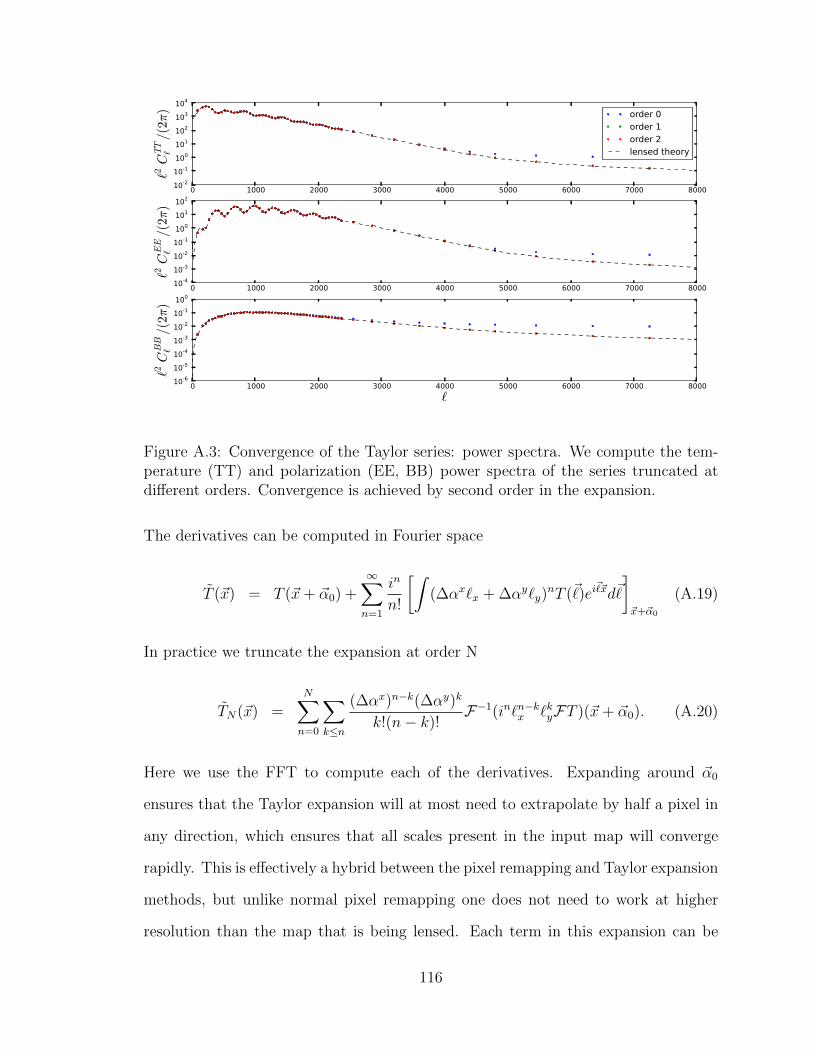
Figure A.3: Convergence of the Taylor series: power spectra. We compute the tem-perature (TT) and polarization (EE, BB) power spectra of the series truncated atdifferent orders. Convergence is achieved by second order in the expansion.

The derivatives can be computed in Fourier space

T (~x) = T (~x+ ~α0) +∞∑n=1

in

n!

[∫(∆αx`x + ∆αy`y)

nT (~)ei~~xd~

]~x+~α0

(A.19)

In practice we truncate the expansion at order N

TN(~x) =N∑n=0

∑k≤n

(∆αx)n−k(∆αy)k

k!(n− k)!F−1(in`n−kx `kyFT )(~x+ ~α0). (A.20)

Here we use the FFT to compute each of the derivatives. Expanding around ~α0

ensures that the Taylor expansion will at most need to extrapolate by half a pixel in

any direction, which ensures that all scales present in the input map will converge

rapidly. This is effectively a hybrid between the pixel remapping and Taylor expansion

methods, but unlike normal pixel remapping one does not need to work at higher

resolution than the map that is being lensed. Each term in this expansion can be

116

computed at the cost of (n + 1) FFT. When expanding around ~α0, we find that the

series converges rapidly. In Figure A.2 we show the pixel histograms of a part of the

maps for each of the first 6 terms in the expansion. We find that the contribution

falls by a factor of ∼ 60 for each order for a 13×13 lensed noiseless CMB simulation

with 0.5’ pixel size.

We also computed the bias for each order using 60 such simulations, shown in

Figure A.3, and found that truncating the series at second order is an excellent ap-

proximation for any realistic CMB experiment. For comparison, the old method of

expanding around ~α = 0 requires more than 20 orders to converge at this resolution,

which given the quadratic scaling of the method corresponds to a performance dif-

ference of a factor of ∼ 50. Using this method, lensing a 13 × 13 patch of the sky

at 0.5’ resolution takes only a few seconds on one processor, and only requires a few

times the memory that a single map takes up. While the method is formulated in the

context of the flat sky in this case, it also generalizes trivially to the full, curved sky.

A.5 Implementation on realistic observations

High resolution ground-based experiments are observing small patches of the sky,

measuring both the temperature and polarization of the CMB. There are also a set

of lower resolution experiments underway targeting larger regions of sky in order to

constrain or measure gravitational waves, but these will require analysis on the curved

sky. In this section we test our power spectrum estimation method on simulated

data, using a specific example of a subset of observations expected from the ACTPol

experiment where the flat-sky approximation is appropriate.

Here we assume that 4 patches of the sky, for a total area of ∼ 300 deg2, are

observed to a noise level of 5.7 µK/arcmin in temperature. The expected coverage

of a patch is non-uniform due to the scanning strategy of the telescope; the expected

117

Figure A.4: Realization of the noise, for a U and Q map (centre and right) generatedusing a simulated pixel weight map (left). This represents the number of observationsper pixel for an inhomogeneous survey, and is taken from a simulation for the ACTPolexperiment.

statistical weight associated with each pixel is shown in the left panel of Figure A.4

for one of the patches. ACTPol will also target a larger region of the sky. For com-

parison, the PolarBear experiment is targeting three 225 deg2 regions at 6 µK/arcmin

sensitivity in temperature [17], and SPTPol have initially targeted a 100 deg2 region,

with the goal to cover 625 deg2 to 5 µK/arcmin [2].

A.5.1 Estimated power spectra

We simulate data for each patch of sky in four subsets, generating independent maps

of identical coverage and equal depth as in Das et al. [12, 11]. We refer to each subset

as a ‘split’. We convolve the simulation with a spherically symmetric gaussian beam

with FWHM of 1′, and we simulate an inhomogeneous noise realization by convolving

the weight map for each patch with a 5.7 µK/arcmin noise realization. We ‘prewhiten’

the temperature maps as defined in Das, Hajian & Spergel [10]. Here, the maps are

convolved in real space with kernels designed to make the power spectrum as flat as

possible, to reduce aliasing of power due to the point source mask. We then apply a

5’ (apodized with a 0.3 cosine kernel) point source mask to account for the possible

contamination from polarized extragalactic point sources.

118

We compute the binned cross-power spectrum CiX×jYb between maps i and j,

for polarization types X and Y , using the pure estimators for B (Eqn. A.11) and

a standard Fourier transform for T and E as discussed in section 2. The estimated

spectrum is then given by

CiX×jYb =

∑b′

MXYbb′ C

iX×jYb′ , (A.21)

where the mode coupling matrix is

MXYbb′ =

∑~,~′

Pb~|WXY (~− ~′)|2

(`′

`

)βXY

(FXY`′ )2Q~′b′ . (A.22)

Here βXY = 2[δBX + δBY ], i.e., for the pure-mode BB spectrum β = 4, but β = 0

for TT and EE. The window function WXY (~) is a product of the point source mask,

the nobs weight map, and a 0.7 cosine apodization at the edges (Smith & Zaldarriaga

[23]), with a geometrical correction for the E modes (Eqn. A.7). The function FXY`

is the product of the beam, a pixel window function and the transfer function of the

prewhitener for the temperature power spectrum. Here Pb~ is a binning matrix, and

Q~b is an interpolation matrix, the binning being defined as a set of annuli in the 2

dimensional power spectrum space. Here we choose a minimal bin size of ∆` = 100.

Each of the mode coupling matrices is computed exactly and inverted in order to

recover an unbiased spectrum.

We compute the spectra for 720 realizations of the noise and CMB, each with a

different realization of the gravitational lensing potential. The cosmological model we

use is the best-fitting ΛCDM model with no tensor contribution, so the B-mode signal

comes only from gravitational lensing. The mean recovered spectra for TT, EE, BB,

and the cross-correlation spectra are shown in Figure A.5, together with the estimated

1σ error bar for a single realization derived from the scatter of the simulations. The

119

Figure A.5: Power spectra estimated from temperature and polarization maps. Thisshows the average binned spectra estimated from 720 Monte Carlo simulations, witherrors estimated from the 1σ dispersion. The B-mode spectra are derived using thepure estimator, to avoid leakage from the E-mode spectrum.

recovered power spectra are consistent with the input power spectra at the 0.1 σ level

in the interval 500 < ` < 6000.

A.5.2 Power spectrum uncertainties

Using the Monte Carlo simulations, we can compare the errors derived from the

internal scatter, with an analytic estimate. This provides a measure of the optimality

of this method. The analytic covariance in a single bin assuming no leakage is given

by

Θ(X×Y );(W×Z)bb =

1

νb

(CX×Wb CY×Z

b + CX×Zb CY×W

b

)+

1

νbnd

(CX×Wb NY×Z

b + CY×Zb NX×W

b + CX×Zb NY×W

b + CY×Wb NX×Z

b

)+

1

νbnd(nd − 1)

(NX×Wb NY×Z

b +NX×Zb NY×W

b

), (A.23)

120

where nd is the number of splits and νb is the number of modes per bin, corrected

for the effect of the window function. CY×Zb is the theoretical power spectrum, and

NY×Zb is the noise power spectrum, given by CY×Z

b,auto − CY×Zb,cross. The derivation of this

expression is given in the Appendix. This does not include the non-Gaussian part

of the covariance due to the effect of lensing, described in Benoit-Levy, Smith & Hu

[4]. This is a subdominant part of the error for the noise levels we consider here, but

introduces correlations between bins. We find that the analytic error bars agree with

the 1σ dispersion from the simulations at the 15% level for 500 < ` < 6000, as shown

in Figure A.6, indicating that all sources of leakage on these scales are subdominant.

The error is dominated by cosmic variance at large scales, but at smaller scales is

noise dominated. This agreement is promising and demonstrates the power of the

pure estimator to recover the B-mode spectrum. In practice these spectra will be

used to construct a likelihood for testing cosmological models, such that

−2 lnL = (Cb − Cthb )TQ−1(Cb − Cth

b ). (A.24)

The full covariance matrix, Q, can be estimated numerically from the simulations, or

analytically, and the binned theory spectra Cthb computed using bandpower window

functions. The realistic likelihood will also include the lensing deflection spectrum,

estimated from higher point statistics of the map, and appropriate cross-correlations.

A.6 Conclusions

A number of issues arise in the analysis of high resolution CMB polarization maps, one

of the most significant being the leakage of E-mode into B-mode polarization due to

observing a limited region of sky. In this appendix we have described a simple method

for estimating the power spectrum in the flat sky approximation that minimizes this

leakage. It draws on an existing all-sky method using a ‘pure’ estimator for the

121

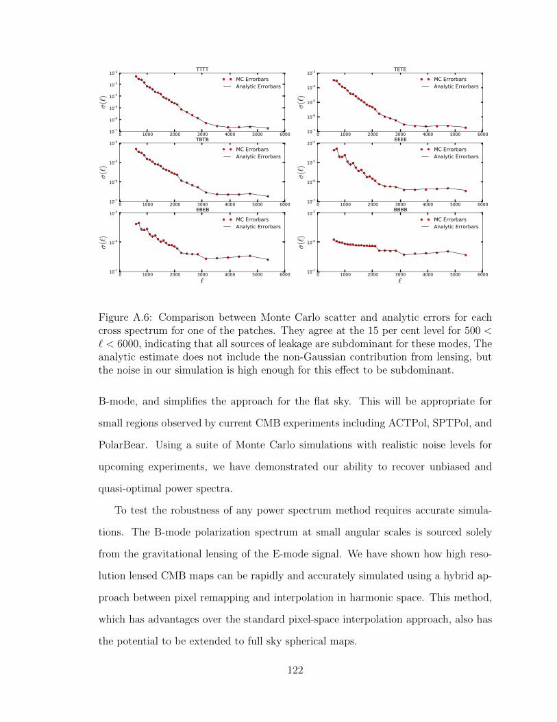
Figure A.6: Comparison between Monte Carlo scatter and analytic errors for eachcross spectrum for one of the patches. They agree at the 15 per cent level for 500 <` < 6000, indicating that all sources of leakage are subdominant for these modes, Theanalytic estimate does not include the non-Gaussian contribution from lensing, butthe noise in our simulation is high enough for this effect to be subdominant.

B-mode, and simplifies the approach for the flat sky. This will be appropriate for

small regions observed by current CMB experiments including ACTPol, SPTPol, and

PolarBear. Using a suite of Monte Carlo simulations with realistic noise levels for

upcoming experiments, we have demonstrated our ability to recover unbiased and

quasi-optimal power spectra.

To test the robustness of any power spectrum method requires accurate simula-

tions. The B-mode polarization spectrum at small angular scales is sourced solely

from the gravitational lensing of the E-mode signal. We have shown how high reso-

lution lensed CMB maps can be rapidly and accurately simulated using a hybrid ap-

proach between pixel remapping and interpolation in harmonic space. This method,

which has advantages over the standard pixel-space interpolation approach, also has

the potential to be extended to full sky spherical maps.

122

A.7 Acknowledgements

We thank David Spergel and Jeff McMahon for useful discussions and Mike Nolta for

providing simulated coverage for the upcoming ACTPol experiment. SD acknowledges

support from the David Schramm Fellowship at Argonne National Laboratory and

the Berkeley Center for Cosmological Physics fellowship. Funding from ERC grant

259505 supports JD, TL and SN.

A.8 Error Calculation

Here we derive an analytic expression for the expected error bars on each of the

cross-power spectrum, X, Y, W and Z stand for T, E and B. The variance is given by

Θ(X×Y );(W×Z)bb = 〈(C(X×Y )

b − 〈C(X×Y )b 〉)(C(W×Z)

b − 〈C(W×Z)b 〉)〉

=1

N

1

ν2b

nd∑i,j,k,l

∑~∈b

∑~′∈b

(⟨X∗i~ Y

j~W

∗k~′ Z

l~′

⟩−⟨C

(iX×jY )b

⟩⟨C

(kW×lZ)b

⟩)× (1− δij)(1− δkl). (A.25)

The Kronecker symbol removes the auto power spectra. nd represents the number

of splits we are cross correlating and νb the number of modes in the annuli b. The

general normalization is

N =

nd∑i,j,k,l

(1− δij)(1− δkl) =

nd∑i,j,k,l

(1− δij − δkl + δijδkl) = n4d − 2n3

d + n2d. (A.26)

Applying Wick’s theorem,

Θ(X×Y );(W×Z)bb =

1

N

1

νb

nd∑i,j,k,l

[⟨C

(iX×kW )b

⟩⟨C

(jY×lZ)b

⟩+⟨C

(iX×lZ)b

⟩⟨C

(jY×kWb

⟩]× (1− δij)(1− δkl). (A.27)

123

We can decompose the estimated power spectrum into signal and noise, such that

⟨C

(iX×kW )b

⟩= CX×W

b + δikNX×Wb , (A.28)

and then we can decompose Θ(X×Y );(W×Z)bb in three terms

Θ(X×Y );(W×Z)bb =

1

νb

(CX×Wb CY×Z

b + CX×Zb CY×W

b

)+

1

N

1

νb

nd∑i,j,k,l

(CX×Wb δjlN

Y×Zb + CY×Z

b δikNX×Wb + CX×Z

b δjkNY×Wb + CY×W

b δilNX×Zb

)× (1− δij)(1− δkl)

+1

N

1

νb

nd∑i,j,k,l

(δikN

X×Wb δjlN

Y×Zb + δilN

X×Zb δjkN

Y×Wb

)× (1− δij)(1− δkl). (A.29)

Finally, using

nd∑i,j,k,l

δjl (1− δij − δkl + δijδkl) = n3d − 2n2

d + nd, (A.30)

and

nd∑i,j,k,l

δikδjl (1− δij − δkl + δijδkl) = n2d − nd, (A.31)

the variance is given by

Θ(X×Y );(W×Z)bb =

1

νb

(CX×Wb CY×Z

b + CX×Zb CY×W

b

)+

1

νbnd

(CX×Wb NY×Z

b + CY×Zb NX×W

b + CX×Zb NY×W

b + CY×Wb NX×Z

b

)+

1

νbnd(nd − 1)

(NX×Wb NY×Z

b +NX×Zb NY×W

b

). (A.32)

124

References

[1] Ade P., et al., 2013, arXiv:1303.5075

[2] Austermann J., Aird K., Beall J., Becker D., Bender A., et al., 2012, Proc. SPIE,

8452, 84520E

[3] Bennett C., Larson D., Weiland J., Jarosik N., Hinshaw G., et al., 2012

[4] Benoit-Levy A., Smith K. M., Hu W., 2012, Phys.Rev., D86, 123008

[5] Bond J., Jaffe A. H., Knox L., 1998, Phys.Rev., D57, 2117

[6] Born M., Wolf E., 1980, Principles of Optics Electromagnetic Theory of Propa-

gation, Interference and Diffraction of Light

[7] Bowyer J., Jaffe A. H., Novikov D. I., 2011, MasQU: Finite Differences on Masked

Irregular Stokes Q, U Grids. Astrophysics Source Code Library

[8] Bunn E. F., 2011, PRD, 83, 083003

[9] Cao L., Fang L.-Z., 2009, Astrophys.J, 706, 1545

[10] Das S., Hajian A., Spergel D. N., 2009, Phys. Rev. D, 79, 083008

[11] Das S., Louis T., Nolta M. R., Addison G. E., Battistelli E. S., et al., 2013

[12] Das S., Marriage T. A., Ade P. A., Aguirre P., Amir M., et al., 2011, Astrophys.J.,

729, 62

125

[13] Grain J., Tristram M., Stompor R., 2009, PRD, 79, 123515

[14] Grain J., Tristram M., Stompor R., 2012, PRD, 86, 076005

[15] Hinshaw G., et al., 2003, Astrophys.J.Suppl., 148, 135

[16] Kamionkowski M., Kosowsky A., Stebbins A., 1997, Phys.Rev., D55, 7368

[17] Kermish Z., Ade P., Anthony A., Arnold K., Arnold K., et al., 2012

[18] Lewis A., 2005, Phys.Rev., D71, 083008

[19] Lewis A., Challinor A., Turok N., 2002, PRD, 65, 023505

[20] Niemack M., Ade P., Aguirre J., Barrientos F., Beall J., et al., 2010, Proc. SPIE,

7741, 77411S

[21] Seljak U., Zaldarriaga M., 1997, Phys.Rev.Lett., 78, 2054

[22] Smith K. M., 2006, Phys.Rev., D74, 083002

[23] Smith K. M., Zaldarriaga M., 2007, Phys.Rev., D76, 043001

[24] Story K., Reichardt C., Hou Z., Keisler R., Aird K., et al., 2012

[25] Zhao W., Baskaran D., 2010, PRD, 82, 023001

126

Appendix B

Methods for CMB Lensing

Estimation without Sensitivity to

Foregrounds

B.1 Lensing Biases from Foregrounds

Foreground sources such as SZ clusters, radio sources and dusty sources all induce sig-

nal into CMB temperature maps. As lensing estimation uses a quadratic combination

of temperature modes, the foregrounds signals persist in the estimated lensing map,

albeit in an altered form due to their processing through the lensing estimator. This

contamination can cause biases in both CMB lensing auto- and cross-correlations

(see e.g. Chapter 3 or [1, 2, 3, 4, 5]). In both cases, the source of these biases

is the fact that foreground sources introduce a spurious part into the temperature

four-point-function (relevant for measurements of the lensing power spectrum) and

the galaxy/tracer-temperature-temperature three-point function (relevant for cross

correlation).

127

More concretely, for the quadratic estimator

φ(L) =

∫d2l

(2π)2f(l,L)T (l)T (L− l), (B.1)

the foreground sources, which we take to contribute an amount P (n) to the observed

temperature map, cause a bias in lensing power spectrum measurements of

∫d2l

(2π)2

d2l′

(2π)2f(l,L)f(l′,L) 〈P ∗(l)P ∗(L− l)P (l′)P (L− l′)〉 (B.2)

plus additional terms consisting of four-point functions involving both P and the

true CMB temperature T .

Similarly, foreground sources can bias cross-correlations of a mass-tracer density

field g(n) with CMB lensing by

∫d2l

(2π)2f(l,L) 〈P (l)P (L− l)g∗(L)〉 (B.3)

B.2 Immunizing the Lensing Estimator to Fore-

ground Contamination

B.2.1 Poisson Foregrounds

For many contaminants (e.g. radio sources or the cosmic infrared background), a

dominant form of these contamination four- and three-point functions are the Poisson

or 1-halo contributions. These contributions are also the simplest to treat analytically

as they are approximately constant (C or D respectively) over relevant scales, i.e.

〈P (l)P (L− l)g∗(L)〉conn = C; 〈P ∗(l)P ∗(L− l)P (l′)P (L− l′)〉conn = D. (B.4)

128

The fact that Poisson-distributed fields have a constant four- or three-point func-

tion can be seen by considering the constant Fourier transform of random distributions

of delta functions.

We would like to modify the existing lensing reconstruction procedure so that the

biases from Poisson foregrounds are removed. To remove biases in cross-correlations

and reduce the biases in auto-correlations, it can be seen (by setting the correlation

functions in Eqs. (B.2) and (B.3) to a constant) that the following simple foreground

immunization condition must be satisfied by the reconstruction weight function f :

F [f ] ≡∫

d2l

(2π)2f(l,L) = 0 (B.5)

We now rederive a modified lensing estimator with a new weight function f ,

which has the least possible variance given that it must now satisfy the immunization

condition. This additional condition can easily be incorporated in the estimator

variance-minimization formalism described in Chapter 2.

In Chapter 2, we show that the variance of the conventional quadratic estimator

for the lensing potential is given by

V [f ](L) = 2

∫d2l

(2π)2f 2(l,L)ClC|L−l| (B.6)

and that the requirement that the estimator be unbiased implies that

I[f ] ≡∫

d2l

(2π)2f(l,L)K(l,L) = 1 (B.7)

where

K(l,L)φ(L) =[(L− l) ·L Cl−L + l ·L Cl

]φ(L) (B.8)

and tildes denote unlensed, noiseless power spectra.

129

To derive the estimator in the absence of foregrounds, we calculated the esti-

mator weight function f by minimizing V [f ] − λI[f ]. We now derive a modified f

which reduces foreground sensitivity by adding a new Lagrange multiplyer µ for the

foreground immunization condition and minimizing

V [f ]− λI[f ]− µF [f ] (B.9)

with the additional constraint equations I = 1; F = 0.

We obtain the following expression for the minimum variance f which still satisfies

the foreground immunization condition:

f(l,L) =K(l,L)−Q(L)

2C`C|L−l|H(L) (B.10)

where

H(L) =

[∫d2l

(2π)2

(K(l,L)−Q(L))K(l,L)

2C`C|L−l|

]−1

(B.11)

and

Q(L) =

∫d2l

(2π)2K(l,L)

2C`C|L−l|∫d2l

(2π)21

2C`C|L−l|

(B.12)

This expression can be easily explained. Neglecting for a moment the normaliza-

tion factor H, in this estimator one is simply subtracting a term Q/2C`C|L−l| from the

filter function, i.e. a constant in l over inverse power spectrum weights. This is exactly

the optimal estimator to estimate the level of a constant three-point function. Essen-

tially the additional term is just an estimator for the level of the connected/constant

part multiplied by an integral (the numerator of Q) giving the response of the usual

lensing estimator to a constant three point function; i.e. this expression estimates

the level of contamination, calculates its effect on the usual lensing estimator and

subtracts this contamination off from the original estimate. The normalization is

also modified; this is due to the fact that the estimator for the constant three-point

130

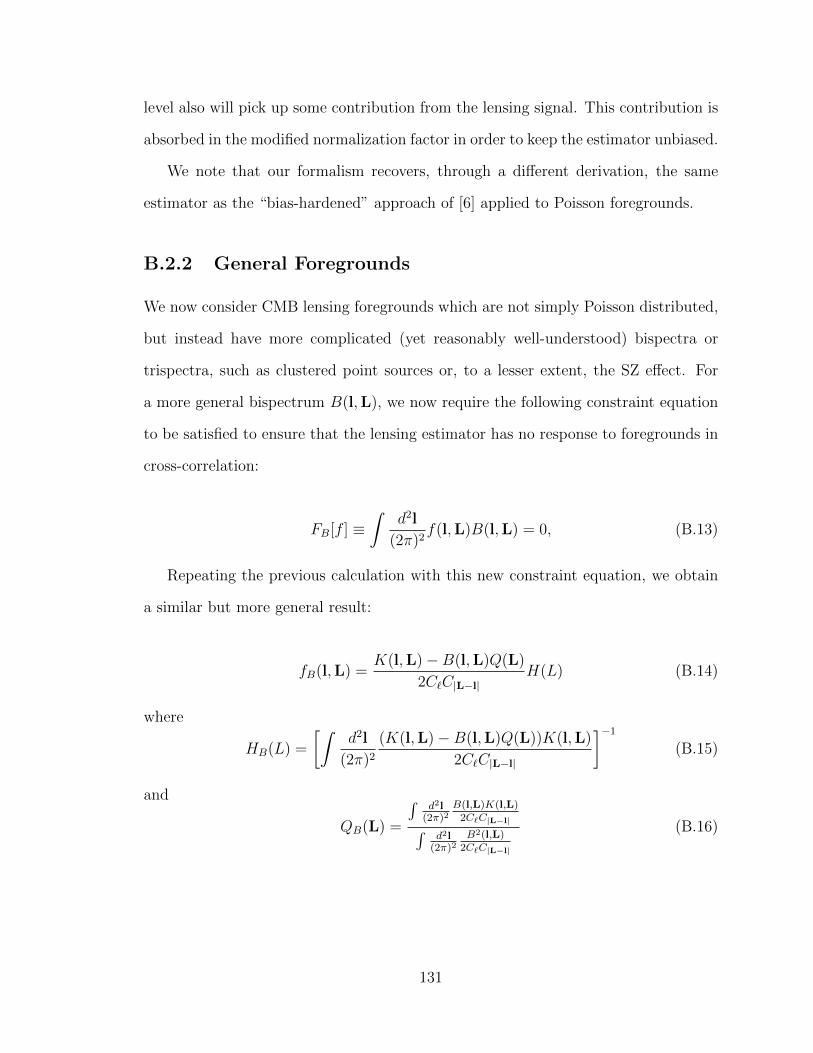
level also will pick up some contribution from the lensing signal. This contribution is

absorbed in the modified normalization factor in order to keep the estimator unbiased.

We note that our formalism recovers, through a different derivation, the same

estimator as the “bias-hardened” approach of [6] applied to Poisson foregrounds.

B.2.2 General Foregrounds

We now consider CMB lensing foregrounds which are not simply Poisson distributed,

but instead have more complicated (yet reasonably well-understood) bispectra or

trispectra, such as clustered point sources or, to a lesser extent, the SZ effect. For

a more general bispectrum B(l,L), we now require the following constraint equation

to be satisfied to ensure that the lensing estimator has no response to foregrounds in

cross-correlation:

FB[f ] ≡∫

d2l

(2π)2f(l,L)B(l,L) = 0, (B.13)

Repeating the previous calculation with this new constraint equation, we obtain

a similar but more general result:

fB(l,L) =K(l,L)−B(l,L)Q(L)

2C`C|L−l|H(L) (B.14)

where

HB(L) =

[∫d2l

(2π)2

(K(l,L)−B(l,L)Q(L))K(l,L)

2C`C|L−l|

]−1

(B.15)

and

QB(L) =

∫d2l

(2π)2B(l,L)K(l,L)

2C`C|L−l|∫d2l

(2π)2B2(l,L)

2C`C|L−l|

(B.16)

131

References

[1] Smith, K. M., Zahn, O., & Dore, O. 2007, Phys. Rev. D, 76, 043510

[2] Hirata, C. M., Ho, S., Padmanabhan, N., Seljak, U., & Bahcall, N. A. 2008,

Phys. Rev. D, 78, 043520

[3] van Engelen, A., Keisler, R., Zahn, O., et al. 2012, arXiv:1202.0546

[4] Bleem, L. E., van Engelen, A., Holder, G. P., et al. 2012, arXiv:1203.4808

[5] Planck Collaboration, Ade, P. A. R., Aghanim, N., et al. 2013, arXiv:1303.5077

[6] Namikawa, T., Hanson, D., & Takahashi, R. 2013, Mon. Not. R. Astron. Soc, 431,

609

132