Cosmic Microwave Background

Cosmic Microwave Background

Cosmological Overview/Definitions Temperature Polarization Ramifications

Cosmological Overview/Definitions Temperature Polarization Ramifications

Scott DodelsonAcademic Lecture V

Goal: Explain the Physics and Ramifications of this

Plot

Goal: Explain the Physics and Ramifications of this

Plot

Coherent picture of formation of structure in the universe

3410 sect

Quantum Mechanical Fluctuations

during Inflation

( )V

Perturbation Growth: Pressure

vs. Gravity

t ~100,000 years

Matter perturbations grow into non-

linear structures observed today

, ,reion dez w

Photons freestream: Inhomogeneities turn into anisotropies

m, r , b , f

Review of NotationReview of Notation

Scale Factor a(t) Conformal time/comoving horizon

dt/a(t) Gravitational Potential Photon distribution Will use Fourier transformsxd3k keikx /(2)3

k is comoving wavenumber Wavelength k-1

Scale Factor a(t) Conformal time/comoving horizon

dt/a(t) Gravitational Potential Photon distribution Will use Fourier transformsxd3k keikx /(2)3

k is comoving wavenumber Wavelength k-1

Photon DistributionPhoton Distribution

Distribution depends on position x (or wavenumber k), direction n and time t (or η).

Moments

Monopole:

Dipole:

Quadrupole:

You might think we care only about at our position because we can’t measure it anywhere else, but …

Distribution depends on position x (or wavenumber k), direction n and time t (or η).

Moments

Monopole:

Dipole:

Quadrupole:

You might think we care only about at our position because we can’t measure it anywhere else, but …

We see photons today from last scattering surface at

z=1100

We see photons today from last scattering surface at

z=1100

D* is distance to last scattering surface

accounts for redshifting out of

potential well

Can rewrite as integral over Hubble radius (aH)-1

Can rewrite as integral over Hubble radius (aH)-1

Perturbations outside the

horizon

Perturbations can be decomposed into Fourier

modes

Perturbations can be decomposed into Fourier

modes

+

=

Combine Fourier Modes to Produce Structure in our

Universe

Combine Fourier Modes to Produce Structure in our

Universe+

=

+ =

In this simple example, all modes have same

wavelength/frequency

In this simple example, all modes have same

wavelength/frequency

More generally, at each wavelength/frequency, need to average over many modes to get spectrum

Inflation produces perturbations

Inflation produces perturbations

Quantum mechanical fluctuations in gravitational potential (k)k’k-k’Pk

Inflation stretches wavelength beyond horizon: k,tbecomes constant

Infinite number of independent perturbations w/ independent amplitudes

Quantum mechanical fluctuations in gravitational potential (k)k’k-k’Pk

Inflation stretches wavelength beyond horizon: k,tbecomes constant

Infinite number of independent perturbations w/ independent amplitudes

Evolution of FluctuationsEvolution of Fluctuations

To see how perturbations evolve, need to solve an infinite hierarchy of coupled

differential equations

To see how perturbations evolve, need to solve an infinite hierarchy of coupled

differential equations

Perturbations in metric induce photon, dark matter perturbations

Evolution upon re-entryEvolution upon re-entry

Pressure of radiation acts against clumping

If a region gets overdense, pressure acts to reduce the density: restoring force

Similar to height of guitar string (pressure replaced by tension)

Pressure of radiation acts against clumping

If a region gets overdense, pressure acts to reduce the density: restoring force

Similar to height of guitar string (pressure replaced by tension)

Before recombination, electrons and photons are tightly coupled:

equations reduce to

Before recombination, electrons and photons are tightly coupled:

equations reduce to

Displacement of a string

Temperature perturbation

Very similar to …

What spectrum is produced by a stringed

instrument

What spectrum is produced by a stringed

instrument

C string on a ukulele

Compare the ukulele spectrum to CMB

spectrum

Compare the ukulele spectrum to CMB

spectrum

CMB is different because …

CMB is different because …

Fourier Transform of spatial, not temporal, signal

Time scale much longer (400,000 yrs vs. 1/260 sec)

No finite length: all k allowed!

Fourier Transform of spatial, not temporal, signal

Time scale much longer (400,000 yrs vs. 1/260 sec)

No finite length: all k allowed!

Largest Wavelength/Smallest Frequency

Smallest Wavelength/Largest Frequency

Why peaks and troughs?Why peaks and troughs? Vibrating String:

Characteristic frequencies because ends are tied down

Temperature in the Universe: Small scale modes enter the horizon earlier than large scale modes

Vibrating String: Characteristic frequencies because ends are tied down

Temperature in the Universe: Small scale modes enter the horizon earlier than large scale modes

The spectrum at last scattering is:

The spectrum at last scattering is:

Θ0 + Ψ ~ cos[k rs(η*) ] Peaks at k = nπ/rs(η*)

One more effect: Damping on small scales

One more effect: Damping on small scales

But

So

On scales smaller than D (or k>kD) perturbations are

damped

On scales smaller than D (or k>kD) perturbations are

damped

Fourier transformof temperature atLast Scattering Surface

Anisotropy spectrum

today

Cl simply related to [0+]RMS(k=l/D*)

Remember that at anywavelength, we are averaging over many modes with different direction.

Puzzle: Why are all modes in phase?

Puzzle: Why are all modes in phase?

The perturbation corresponding to each mode can either have zero initial velocity or zero initial amplitude

We implicitly assumed that every mode started with zero velocity.

Interference could destroy peak structure

Interference could destroy peak structure

There are many, many modes with similar values of k. All have different initial amplitude.

But all are in phase.

First Peak

An infinite number of ukuleles are synchronized

An infinite number of ukuleles are synchronized

Similarly, all modes

corresponding to first trough are in phase: they all have

zero amplitude at

recombination

Without synchronization:Without synchronization:

First “Peak” First “Trough”

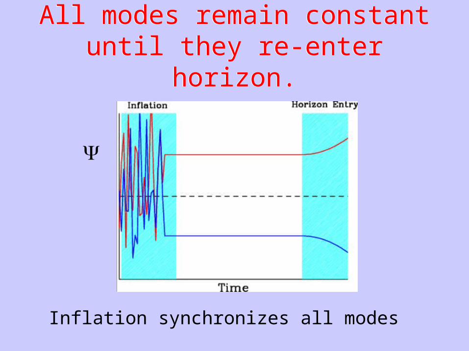
All modes remain constant until they re-enter horizon.All modes remain constant until they re-enter horizon.

Inflation synchronizes all modes

How do inhomogeneities at last scattering show up as anisotropies

today?

How do inhomogeneities at last scattering show up as anisotropies

today?

Perturbation w/ wavelength k-1 shows up as anisotropy on angular scale ~k-1/D* ~l-1

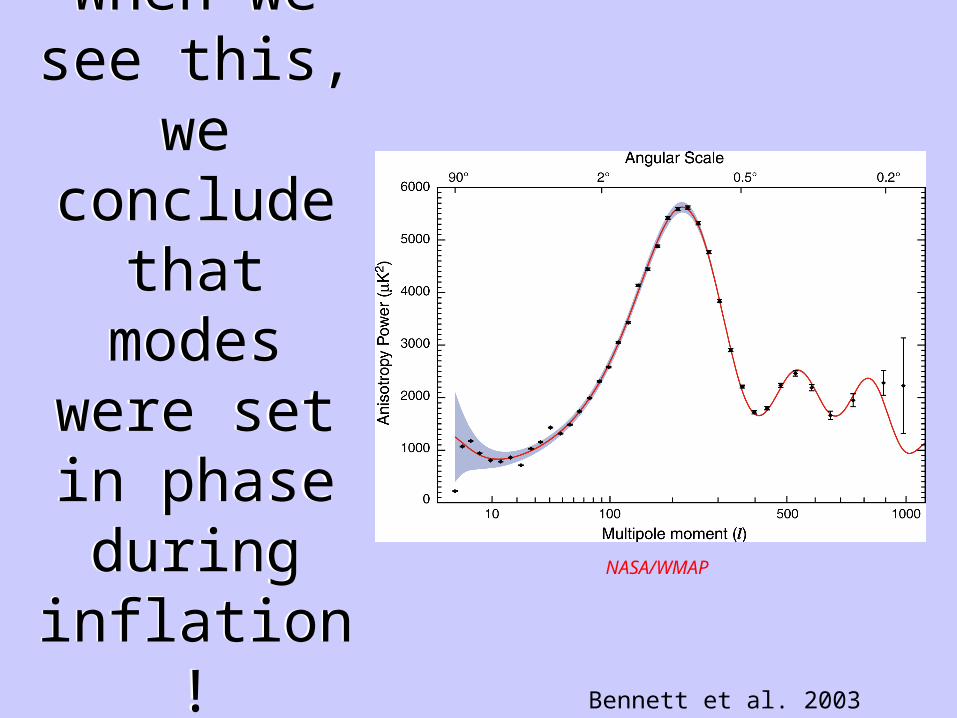
When we see this,

we conclude

that modes

were set in phase during

inflation!

When we see this,

we conclude

that modes

were set in phase during

inflation!Bennett et al. 2003

NASA/WMAP

Compton Scattering produces polarized

radiation field

Compton Scattering produces polarized

radiation field

B-mode smoking gun signature of tensor perturbations, dramatic proof of inflation... We will focus on E.

Polarization field decomposes into 2-modes:

Three Step argument for <TE>

Three Step argument for <TE>

E-Polarization proportional to quadrupole

Quadrupole proportional to dipole

Dipole out of phase with monopole

E-Polarization proportional to quadrupole

Quadrupole proportional to dipole

Dipole out of phase with monopole

Isotropic radiation

field produces

no polarizatio

n after Compton scattering

Isotropic radiation

field produces

no polarizatio

n after Compton scattering

Modern CosmologyAdapted from Hu & White 1997

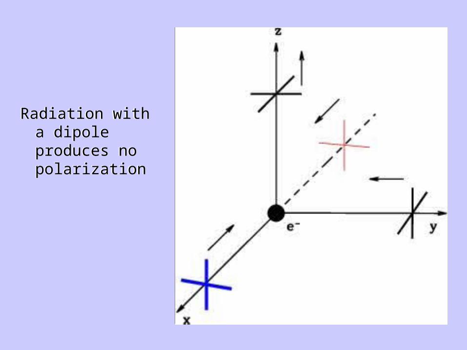
Radiation with a dipole produces no polarization

Radiation with a dipole produces no polarization

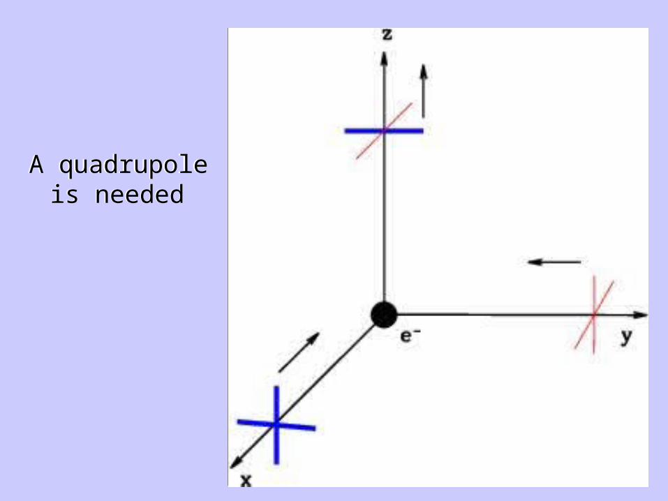
A quadrupole is needed

A quadrupole is needed

Quadrupole proportional to dipole

Quadrupole proportional to dipole

( )ee MFP

vv

x

( )ee MFP

vv

x

Dipole is out of phase with monopoleDipole is out of phase with monopole

1 00vt

0 * *

1 * *

( , ) cos[ ( )]

( , ) sin[ ( )]s

s

k A kr

k B kr

Roughly,

The product of monopole and dipole is initially positive (but small, since dipole vanishes as k goes to zero); and then

switches signs several times.

DASI initially detected TE signal

DASI initially detected TE signal

Kovac et al. 2002

WMAP has indisputable evidence that monopole and dipole are out of

phase

WMAP has indisputable evidence that monopole and dipole are out of

phase

This is most remarkable for scales around l~100, which were not in causal contact at recombination.

NASA/WMAP

Different Geometries Possible

Different Geometries Possible

Inflation predicts a flat universe

We now have a solid argument that the total

density is flat

We now have a solid argument that the total

density is flat Object with known physical size

Parameter I: CurvatureParameter I: Curvature

Same wavelength subtends smaller angle in an open universe Peaks appear on smaller scales in open universe

Hot/cold spots of known physical size has been

observed

Hot/cold spots of known physical size has been

observed

Angular size demonstrates flatness

Angular size demonstrates flatness

Parameters IIParameters II

Reionization lowers the signal on small scales

A tilted primordial spectrum (n<1) increasingly reduces signal on small scales

Tensors reduce the scalar normalization, and thus the small scale signal

Reionization lowers the signal on small scales

A tilted primordial spectrum (n<1) increasingly reduces signal on small scales

Tensors reduce the scalar normalization, and thus the small scale signal

n is degenerate w/ reionization, but polarization pins down the latter: we now know n to within a few percent.

Parameters IIIParameters III Baryons accentuate

odd/even peak disparity

Less matter implies changing potentials, greater driving force, higher peak amplitudes

Cosmological constant changes the distance to LSS

Baryons accentuate odd/even peak disparity

Less matter implies changing potentials, greater driving force, higher peak amplitudes

Cosmological constant changes the distance to LSS

E.g.: Baryon densityE.g.: Baryon density

2x x F Here, F is forcing term due to gravity.

3(1 3 / 4 )s

b

kkc

As baryon density goes up, frequency goes down. Greater odd/even peak disparity.

Bottom lineBottom lineh often used instead of

2 2

21 m bh h

h

CMB data says matter density is only 30% of critical: Need Dark Energy and Dark Matter

ConclusionsConclusions Strong evidence for inflation from CMB

anisotropy/polarization spectra Baryon and matter densities tightly

constrained, consistent with other determinations. Dark energy & dark matter needed

Connection between particle physics & cosmology (inflation, dark matter, dark energy) more solid than ever. We need new tools …

Strong evidence for inflation from CMB anisotropy/polarization spectra

Baryon and matter densities tightly constrained, consistent with other determinations. Dark energy & dark matter needed

Connection between particle physics & cosmology (inflation, dark matter, dark energy) more solid than ever. We need new tools …

Available at www.amazon.com