MPRAMunich Personal RePEc Archive

Corruption and Media Concentration: APanel Data Analysis

Sofiane Cherkaoui Malki

24 August 2017

Online at https://mpra.ub.uni-muenchen.de/81073/MPRA Paper No. 81073, posted 31 August 2017 16:25 UTC

Paris School of Economics M2 Analyse Politique et Economique

Université Paris 1 Panthéon-Sorbonne Master Thesis

UFR 02 Sciences Economiques

CORRUPTION AND MEDIA CONCENTRATION:

A PANEL DATA ANALYSIS

Presented and defended by Sofiane CHERKAOUI MALKI

Under the supervision of Ekaterina ZHURAVSKAYA

Abstract

My master thesis studies the relationship between media concentration and corruption based

on a panel data analysis, with a panel dataset which provides information about 29 countries over a

span of 19 years. Based on a cross-section analysis Djankov, McLiesh, Nenova and Shleifer (2003,

JLE) which focused on the relationship between corruption and media state-ownership, I enhance their

results thanks to panel data fixed effects, to control for more unobservable effects, and several

robustness checks. As Djankov et al did, we focus on two specific media markets: television (TV) and

daily newspapers. Thanks to new data from the book “Who Owns the World‟s Media?” (Noam, 2016),

I broaden the spectrum of their article to focus on the correlations between corruption and all types of

media concentration (public, private and the industry). I confine their previous results: a positive

correlation is found only for public TV with large shares of the market. In fact, I find a negative

correlation between public TV shares and corruption for lower levels of state-ownership, especially in

the case of developed countries. Contrary to daily newspapers, this result remains after many

robustness checks. I provide evidence that low-levels of state-ownership limit concentration of private

media, reducing the risk of media capture. Indeed, competition within the private sector is found to be

negatively correlated with corruption. Finally, I find weak evidence for a positive correlation between

corruption and media industry concentration in only two cases: when considering all types of media

and when considering TV alone.

Keywords: Bureaucratic Corruption, Media Concentration, Media Capture

JEL Codes: D72, D73, L82

AUGUST 2017

L'Université de Paris I Panthéon-Sorbonne n'entend donner aucune approbation ni désapprobation aux

opinions émises dans ce mémoire ; elles doivent être considérées comme propres à leur auteur.

La Paris School of Economics n'entend donner aucune approbation ni désapprobation aux opinions

émises dans ce mémoire ; elles doivent être considérées comme propres à leur auteur.

Acknowledgements:

I would like to thank warmly my supervisor Ekaterina Zhuravskaya, professor at the PSE.

Without her, this master thesis would not have been possible. I am indebted to her for her support, her

help, and for her patience.

I would also like to thank my friends Noémie Malléjac and Antoine Tonnerre, also students

from the Magistère at Paris 1, for their advice and their support.

Contents:

Introduction 1

Literature Review 3

Press Freedom and Corruption Studies . . . . . . . . . . . . . . . . . . . . . . . . . . . . . . . . 3

Media Industry Concentration and Corruption Studies . . . . . . . . . . . . . . . . . . . . 5

Theoretical Starting Point 7

Datasets and Variables Construction 10

First Hypothesis testing 12

Second Hypothesis testing 18

Conclusion 22

Main Tables 23

Appendix 35

Tables . . . . . . . . . . . . . . . . . . . . . . . . . . . . . . . . . . . . . . . . . . . . . . . . . . . . . . . . 35

Graphs . . . . . . . . . . . . . . . . . . . . . . . . . . . . . . . . . . . . . . . . . . . . . . . . . . . . . . . . 73

References 86

1

Master Thesis

1. Introduction:

Since 2015, the Media Ownership Monitor, created by Reporters without Borders (Reporters sans

frontières, RSF), has been expanding to now reach 10 countries (Cambodia, Colombia, Ghana, Mongolia,

Peru, Philippines, Serbia, Tunisia, Turkey and Ukraine). The goal of this new project is to support media

pluralism and independence by combating and documenting media ownership concentration. Indeed, as they

advocate, media pluralism and independence are both prerequisites for press freedom, which in the end

improves political accountability. Henceforth, media ownership concentration can reinforce corruption, by

limiting press freedom. Indeed, because of its influence on press freedom, media concentration can influence

both extortive corruption and collusive corruption (Brunetti and Weder, 2003). Furthermore, as this RSF

project reminded, the risk is even greater when the state regularly intervenes in media markets (e.g. state-

ownership, links with media owners, etc.).

Actually, economists have already studied and confirmed the potential relationship between

corruption and media concentration. The first study to focus on this issue was made by Djankov , McLiesh,

Nenova, and Shleifer (2003, JLE). Although a positive correlation between corruption, which is defined by

Transparency International as “the abuse of entrusted power for private gains”, and media state-ownership

has been confirmed, this result should be taken with caution: the database is limited and quite old, no

particular robustness checks are displayed, and other studies on the same theme all used Djankov et al

database. Moreover, it is a cross-section analysis, not a panel data analysis.

Therefore, our master thesis will be an improvement of the study by Djankov et al rather than just a

replication. We will use a different database in order to improve the findings in the media concentration –

corruption literature. Fortunately, in 2016, Eli Noam, Professor at the Columbia Business School, and the

International Media Concentration Collaboration published the book “Who Owns the World‟s Media?”

which compiles information about media concentration in 29 countries over a period of more than 20 years

for more than 13 media markets (from news media to platforms and internet media). In particular, they

computed indexes and market shares of ultimate owners (i.e. the shareholder which is the decision-maker in

last resort) for each media market. Although they have some data about the top multinational media

companies, data availability is still too limited for empirical analysis. Hence, we will focus on two media

markets: television and daily newspapers. They were originally the ones chosen by Djankov et al, which

makes sense because they are intuitively more likely to have an impact on the public opinion than other

types of media. For instance, these two types of media are more likely to have an impact on the mindsets of

the population and the decision-makers. As Djankov et al stated: “we focused on newspapers and television

since these are the primary sources of news on political, economic, and social issues” (p. 344). Media

concentration can be defined as a relative increase in the market shares of an ultimate owner on the market:

fewer and fewer ultimate owners having higher and higher market shares levels. So, public and private

media concentration definitions follow this definition too. Furthermore, “public” will be used as a synonym

for “state-owned” and does not refer to publicly traded firms.

The novelty of our study is based on two facts. Firstly, from a positive viewpoint, we provide a

rigorous examination for the findings about the correlation between media concentration and corruption,

based on a larger database and estimation techniques not used before in this field. More particularly, thanks

2

Master Thesis

to a panel data analysis, we are able to use fixed effects: year and country fixed effects allow us to control

for unobservable characteristics which are common to all countries or constant for all years. All previous

studies were cross-sections, so our results will be less biased. Furthermore, thanks to Noam‟s book database,

we are able to differentiate between state ownership concentration, private ownership concentration, and

industry concentration. Secondly, from a normative approach, we provide precise insights and quantitative

criteria for policy-makers. Indeed, subjective measures, which were used for press freedom in a great

majority of previous studies, are based on questionnaires which often can‟t guide policies in a precise

direction or give precise criteria for policies assessments. For instance, in the first category of the economic

subcomponent of the press freedom index from the Freedom House, one of the questions is: “does the state

or public media enjoy editorial independence, and do they provide a range of diverse, nonpartisan

viewpoints?” Without providing a clear definition of editorial independence, it is hard to draw precise

policies about public ownership to improve press freedom. Often, questions are clearer (e.g. “does the state

have a monopoly on any news medium?” in the same category), but the drawbacks are that they are usually

easily and already met by developed countries. It means that these indexes create a helpful tool for

developing countries or new democracies, but when all the first easy criteria are met, it becomes harder for

policy-makers to use results based on these measures. Using hard measures, like public media market shares

or the Herfindhal-Hirschmann Index (HHI) for a whole media market, criteria and policies insights can be

more easily drawn from empirical results.

The two questions will we answer about the relationship between media concentration and

corruption, for the television and the newspapers markets, are based on Djankov et al findings and on a

theory provided by Besley and Prat‟s model (2006). However, as we will show later, this model is just a

starting point for our reasoning because it has some defaults. Is media state-ownership positively correlated

with corruption? Is media industry concentration positively correlated with corruption?

Regarding the first question, we find that only public TV is correlated with corruption. From Noam‟s

book media markets study, we observe that these two markets have only two differences in terms of markets

characteristics: television market is a mass media (in terms of audience) and is based on high fixed costs and

low marginal costs (which leads to higher concentration), but daily newspapers market does not share any of

these features. Hence, at least one of these two characteristics is needed for a specific type of media to create

incentives for the state to consider media capture. However, we cannot distinguish between the two with our

data. Future research should include more media markets, with different levels of viewership and different

levels of fixed costs, in order to distinguish which one of these characteristics incentivizes media capture the

most. Furthermore, we find that public TV is negatively correlated with corruption, and this relationship is

quadratic: after some level of public TV market shares, public TV is positively correlated with corruption.

This surprising result remains after several robustness checks. It can be explained by another finding:

moderate levels of public TV have a pro-competitive impact on the private sector. A possible explanation is

the impact of public TV on the set of strategies of private players: mergers and acquisitions constitute a

profitable strategy for private players facing high fixed costs and low marginal costs. However, this strategy

cannot be used against state-owned media: private players will then have to maintain more competitive

strategies to acquire more market shares. Nevertheless, we don‟t provide causality. In fact, an alternative

explanation could be a correlation due to our time frame. Indeed, thanks to a Chow test, we find that there is

a structural change in 2002: only after this date a negative quadratic relationship between public TV and

corruption is found. Actually, after 2002, the average corruption level and the average public TV shares both

3

Master Thesis

steadily decreased. Furthermore, omitted variable biases can‟t be totally dismissed. However, we can say

that economic freedom, trade openness and especially development are requirements which have to be met

in order to make the relationship between public TV and corruption negative. To conclude, we can answer

positively to the first question only if some conditions are met and if public TV market shares are

sufficiently high. Interestingly, this is not true for low levels of public TV which are negatively correlated

with corruption. So, a global answer to the first question would be no, because the overall impact of public

TV on corruption in the general case is negative.

Regarding the second question, the findings are less clear. If we define media industry concentration

as the average of the HHI for all the 13 media markets, we find no correlation at all. However, total media

industry concentration is likely to be positively correlated with corruption in countries with high defense

expenditures and low levels of trade openness. Therefore, we used HHI variables for the TV market and the

newspapers market separately. As before, the variables for the newspapers market (i.e. the HHI for the

whole newspapers market) do not influence corruption. The industry concentration in the TV market seems

to be positively correlated with corruption under some conditions: extreme levels of public TV sector (very

high or very low levels), low competition in the private sector of the TV market, low level of development,

and high levels of state expenditures, particularly in defense. A possible explanation for the non-significance

comes from the opposite directions of the effects of public TV shares and private concentration regarding

corruption. Indeed, private sector concentration is positively correlated with corruption, and its relationship

with corruption is also quadratic (i.e. decreasing here). Hence, competition within the private sector reduces

corruption. Therefore, the ultimate sign of the total industry concentration will depend on which effect

between public and private concentration dominates. Henceforth, if the TV market is dominated by a private

oligopoly, then total concentration will be positively correlated with corruption. To conclude, we can answer

the second question positively, also under some conditions but these conditions are more likely to be met.

Hence, we can say that we find weak evidence for a positive correlation between media industry

concentration and corruption, especially in the case of the TV market.

This master thesis is structured as follows. The second part is a literature review. The third part

presents a discussion about the first theory on this subject. The fourth part focuses on the choice of datasets

and the variables construction. The fifth and the sixth parts display our results and interpretations

respectively about the tests of first hypothesis and the tests of the second hypothesis. The seventh part is the

conclusion. The eighth part and the ninth part are respectively the main tables and the appendix. The tenth

part contains the references.

2. Literature Review:

2.1 Press Freedom and Corruption Studies:

To begin with, our study is linked to the scientific literature about the relationship between press

freedom and corruption.

4

Master Thesis

The first major empirical study on the subject was the article “A Free Press is Bad News for

Corruption” by Brunetti and Weder (2003, JPE). This study is part of the literature about the impact of

external checks on corruption (e.g. an independent judiciary body). The reasoning is that a free press has

higher incentives to search and control corruption than other independent bodies because of

commercialization: only media outlets make extra profits by publishing corruption scoops. According to the

authors, a free press has the following features: competitive market, free entry in journalism, free entry in

publishing, and freedom from outside pressures (politicians, etc.). In fact, they acknowledge that the impact

of press on corruption is conditional to the production process of the press. The cross-country empirical

analysis is based on the Freedom House different press freedom indexes, which focus on different aspects of

press freedom (law, political environment, and economic environment), and on several subjective measures

of corruption, including the CPI. The authors find that a free press reduces corruption, and this result is

robust to different specifications, different estimation models (OLS and ordered probit estimation

technique), and different measurements. The issue of a possible reverses causality (which could create

endogeneity problems) is checked by estimating the same model without repressive regimes, because

repressive regimes have a better chance to limit press freedom and so it is in those countries that the

probability of reverse causality (i.e. a corrupt regime limiting press freedom) is the highest. A short panel

data analysis provided by the authors also confirms their previous results.

The second significant empirical study on the same issue was the scientific paper called “A

Contribution to the Empirics of Press Freedom and Corruption” by Freille, Haque and Kneller (EJPE, 2007).

The idea is to use the disaggregated measures of press freedom published by the Freedom House and to

apply an Extreme Bound Analysis (EBA) with a database of 51 countries with a time frame of 10 years

(1995 to 2004), in order to check the correlation between press freedom and corruption. The EBA is used as

a robustness check for correlations: the goal is to see whether the results depend on the specifications used.

The idea is to change the controls (in combinations of three in each specification) for every regression until

all the possibilities for controls combinations have been exhausted. Then, the estimates for the main

regressor (press freedom indexes here) are ordered, and the following condition needs to be checked: the

extreme upper bound (i.e. the highest beta plus the double of its standard errors) and the extreme lower

bound (i.e. the lowest beta plus two times its standard errors) are both statistically significant and of the

same sign. It confirmed Brunetti and Weder study regarding the impact of the political environment and the

economic environment of press freedom on corruption. However, the legal environment of press freedom

does not pass the test: its relationship with corruption is insignificant.

Other studies confirm and improve the results found in the two studies cited above. Chowdhury

(2004, EL) added to the existing literature an instrumental variable analysis (with colonial past in terms of

legal system used as an instrument for press freedom) and dynamic panel analysis (based on the Arellano

and Bond dynamic panel data model (1991)) to test the relationship between press freedom and corruption,

and previous studies results were confirmed. Camaj (IJP, 2013) showed that the negative effect of press

freedom on corruption is stronger in countries with higher vertical accountability (i.e. accountability

5

Master Thesis

regarding the civil society) and higher horizontal accountability (i.e. accountability within the state). Hence,

both internal and external controls make a free press more efficient. Moreover, Lindstedt and Naurin

(ISPSR, 2010) investigated the real impact of transparency on corruption, and discovered that a free press

was an efficient institution to increase transparency and reduce corruption (at least more efficient than self-

imposed transparency rules).

However, we will now focus on the two first studies, which are at the center of our analysis, and we

will analyze their limits. The first default would be the lack of data, which is explained by the availability of

data on this subject at the time of the study. Then, the type of measurement is problematic: all the measures

(except the repressive actions count variable) are perception/subjective measures. An issue will be the policy

implications of such results, and these implications are especially not accurate for developed countries. The

commercialization incentives theory can be challenged by the possibility of media capture by the state.

Rightly, the authors remind readers that collusion between the state and all journalists (or enough of them) is

impossible, at least because of coordination failures. However, media capture is still possible because there

is no free entry in publishing. And this fact is likely to last: media markets have high and growing fixed

costs which a key factor for industry concentration (fact number 1 about media characteristics, Noam‟s

book, 2016). Hence, the precise conditions needed for the alignment of journalists‟ incentives and media

outlets owners‟ incentives are not yet totally clear. One of these conditions, according to the results

concerning the economic subcomponent of the press freedom index, seems to be the concentration of media

ownership. Actually, this subcomponent aggregates many different economic aspects of press freedom (e.g.

“the economic situation of a country”, Freedom House Survey, 2008). So, the question of media ownership

relationship with corruption is still not solved with these studies. In fact, other studies have focused on the

impact of this hard measure concerning press market on corruption.

2.2 Media Industry Concentration and Corruption Studies:

The most essential study in this field is the paper named “Who Owns the Media?” by Djankov et al

(2003, JLE). Many papers followed the path of this article and used their database later. For instance, Besley

and Prat (AER, 2006) used their database to test their model about the impact of public media concentration

on corruption. Another example is the study made by Houston et al. (JFE, 2011): they used Djankov et al

database to test the impact of media ownership on corruption in bank lending. Hence, that‟s why it is

important to look at the roots of this literature.

The original goal of their study was to test opposite approaches about state-ownership in the

particular case of media property. Indeed, Djankov et al wanted to confront the public interest (Pigouvian)

theory and the public choice theory regarding state-ownership of media. According to the Pigouvian theory

(Pigou, 1932), there are three reasons justifying the existence of public ownership in media markets. To

6

Master Thesis

begin with, regarding information itself, it is a public good, so the non-exclusivity feature reduces the

possibility of profitability for private owners. Henceforth, state production can help to re-establish allocative

efficiency. Then, the production process is characterized by high fixed costs and low marginal costs, which

creates increasing returns to scale. Hence, if the economies of scale are not used (e.g. if producers are too

many and not big enough), productive efficiency won‟t be reached. Finally, the state-owned media are less

likely to be biased by special interests, at least not in the same way private ultimate owners influence their

media outlets. For instance, these arguments were used to support the existence of the British Broadcasting

Corporation (cf Coase, 1950). The public choice approach would highlight the fact that politicians in power

can also influence the editorial policy of the state-owned media. Moreover, competition within the private

sector should give rise to a sufficient number of media outlets, with different biases and viewpoints, such

that on average information is not biased. Therefore, the authors studied the different consequences of media

state-ownership (including the impact on corruption), and they concluded that the public choice approach

was more likely to be true.

Djankov et al. made a database of the ultimate owners of newspapers and television in 97 countries

in 1999 and 2003. The ultimate owner is defined as the largest shareholder at each level of the chain of

indirect ownership. It is the decision-maker as a last resort. The graph B1 is an example of the construction

of the ultimate owners variable. Here TVN is owned by the Schneider family through different indirect

control deals. They created four categories for the ultimate owners: “the state, families, widely held and

other” (p. 350). In our last example, TVN would be considered as family owned. Two important variables

were created by the authors: the state-ownership by count, which is the ratio of the number of public

newspapers among the five largest newspapers/TV stations, and the state-ownership by share, which

represents the percentage of the top five largest newspapers/TV stations total markets shares that is state-

owned. For instance, the authors found that 2 out of the top five newspapers in the Philippines are public,

and these two public stations have 43.5% of the top five newspapers total market shares. So, the state-

ownership by count would be 40% and the state-ownership by shares would be 43.5%, for the Philippines.

The definition of state-ownership is crucial here: Djankov et al consider that political party ownership is not

state-ownership, even if the political party in question holds power. The part of the article which is the most

important for us is the fifth part of the article about the consequences of state ownership of the media on

political and economic freedom. The authors checked the impact of the state variables on corruption in the

Tables 7 in their article (p.370). Public press is significantly positively correlated with corruption, whereas

the estimates for public TV are negative and insignificant.

Nevertheless, there are some issues with this study, and it explains why an improvement of this study

with a new dataset and a panel data analysis would be useful. Firstly, there is an issue with the dataset: the

time frame is limited to two years, 1997 and 2003, which correspond to the last years of era of privatizations

and opening to competition. Hence, media state-ownership, especially in TV, was still significant in terms of

market shares. Therefore, there might an upward bias in the estimates for TV public ownership: the state

ownership impact on corruption might be overestimated, compared to the true long term relationship

between media public ownership and corruption. Secondly, there is an issue with the variables construction.

Actually, the top five players of a market might not be representative of the whole market: it depends on the

market shares of the outsiders. For instance, having two dominant public firms (so, one dominant ultimate

7

Master Thesis

owner) might have a different impact on corruption if the rest of the market is a competitive fringe or if the

rest of the market is composed of few middle-sized private firms. Their dataset time frame and variables

construction can both lead to an upward bias, which can explain the gap between what they found and what

we found. Actually, without this upward bias, the correlation between public press and corruption could

become insignificant and the correlation between public TV and corruption could become significant (and

still negative), which is precisely what we found. Furthermore, the case of political party ownership is an

interesting example of a larger problem with their variables construction rules. Even though there aren‟t any

clear-cut answers and it should be done on a case by case basis. A media owned by a political party in power

or even by a firm with close ties to the political party in power should be considered as public, because it

will have the same behavior as state-owned media outlets. Anecdotal historical evidence is provided by the

behavior of many politicians while they were in power (e.g. Erdogan or Berlusconi with Mediaset media

group). As a result, state-ownership in their dataset might actually be underestimated because of the

restrictive definition of state-ownership. Finally, there is a problem with the empirical analysis provided by

the authors. Actually, they only used simple Ordinary Least Squares (OLS) regressions in a cross-country

analysis, with only four control variables, and with only 95 observations for each regression. For instance,

the results could be biased by specific factors common for all the countries or constant over time.

Henceforth, the correlations would be biased by using simple OLS.

These are the reasons why a refinement of Djankov et al study will be useful. A theoretical first step

useful for this is the model made by Besley and Prat, who used the Djankov et al database in order to test

their model. Because their model was adapted to Djankov et al data and supported by previous empirical

evidence, we will discuss this model in order to extract testable hypotheses. However, we will also explain

why this model fails to be supported by our empirical findings, and we will give insights about how this

model should be modified in order to be adapted to new empirical evidence. This will help us discuss our

empirical results later.

3. Theoretical Starting Point:

We will now present the theory created by Besley and Prat in order to discuss the impact of media

concentration on corruption.

Firstly, we will rapidly present their model. We have the following set-up. It is a two-period voting

model, where an incumbent in power is seeking for reelection. The incumbent has the type θ, which can be

either good g or bad b. A bad incumbent practices embezzlement and extracts a rent r if he is reelected.

Voters don‟t know these parameters, but there is a probability q that the news outlets (n in number) receive a

signal which demonstrates that the incumbent is of type b. The payoff of the media i is the following:

{

In fact, voters only buy “informative news”, meaning that media outlets sales are different from zero only

when they receive and publish the signal about the bad incumbent in power. The voters are equally

distributed among the newspapers, so if m media outlets publish the signal, each of them receives the sales

8

Master Thesis

revenues . So a is the audience-related revenues when m is equal to 1, so it represents the

commercialization of the media outlets. It is similar to the two rules of Bertrand (1883) competition (equal

shares when equal prices and winning all the market by undercutting). The higher a is, the higher the

incentives to be the one to publish the information. However, the bad incumbent can “bribe” media outlets

owners in order to prevent his real type to be revealed to the public. If his bribery is successful, he can stay

in power for another term. Before the vote and before the publication of the news, the incumbent can

transfer to the media outlet i in order to silence it. However, there is a transaction cost , which makes the

transfer paid by the incumbent become when it arrives to the media outlet i. This is precisely media

capture. However, the authors notice that the transfer is not necessarily direct bribe to the owner of the

media outlet: it can take the form of subsidies or of favorable regulations in other sectors. Then, voters will

vote and will systematically reject bad incumbents, if the information asymmetry is resolved thanks to the

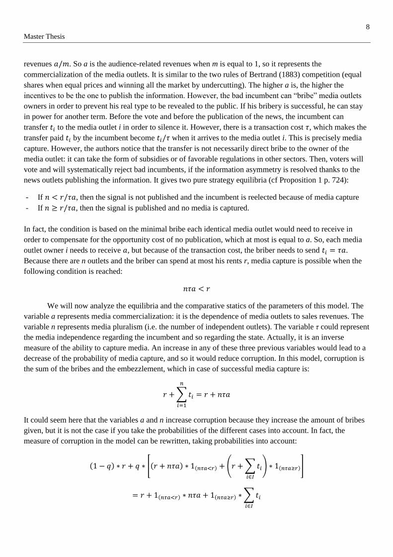
news outlets publishing the information. It gives two pure strategy equilibria (cf Proposition 1 p. 724):

- If , then the signal is not published and the incumbent is reelected because of media capture

- If , then the signal is published and no media is captured.

In fact, the condition is based on the minimal bribe each identical media outlet would need to receive in

order to compensate for the opportunity cost of no publication, which at most is equal to a. So, each media

outlet owner i needs to receive , but because of the transaction cost, the briber needs to send .

Because there are n outlets and the briber can spend at most his rents r, media capture is possible when the

following condition is reached:

We will now analyze the equilibria and the comparative statics of the parameters of this model. The

variable a represents media commercialization: it is the dependence of media outlets to sales revenues. The

variable n represents media pluralism (i.e. the number of independent outlets). The variable τ could represent

the media independence regarding the incumbent and so regarding the state. Actually, it is an inverse

measure of the ability to capture media. An increase in any of these three previous variables would lead to a

decrease of the probability of media capture, and so it would reduce corruption. In this model, corruption is

the sum of the bribes and the embezzlement, which in case of successful media capture is:

∑

It could seem here that the variables a and n increase corruption because they increase the amount of bribes

given, but it is not the case if you take the probabilities of the different cases into account. In fact, the

measure of corruption in the model can be rewritten, taking probabilities into account:

[ ( ∑

) ]

∑

9

Master Thesis

Here, I is the set of media outlets who accepted the bribe even when the information was published. Hence,

we see that the variables a and n will increase the amount of bribes in the case of successful media capture

but they will decrease the probability of it happening by increasing the cost of media capture. In another

version of the model, the authors endogenized the number of outlets by allowing free entry with an entry

cost c. Hence, an increase in the variable c will increase the barriers to entry to the media market, limiting

media pluralism and so increasing the probability of media capture, which would increase corruption.

Finally, we will extract testable hypotheses from this model. Actually, the three variables we are

interested in are c, n, and τ, or more precisely n(c) (n as a function of c) and τ. Indeed, we are interested in

the impact of media industry concentration on corruption and also in the difference between public media

concentration and private media concentration regarding their respective impact on corruption. Total, public

and private media concentration will have an impact on press freedom because market structure and

ownership structure influence the probability of media capture. Regarding state-ownership of media, it could

be modeled here by stating that one media outlet i has a transaction cost : this media outlet i

would be easier to capture, or even free to capture. For instance, it could be argue that the incumbent can

appoint a favorable administrator at the head of the state-owned media outlet, facilitating media capture.

This difference in terms of media independence can be explained by the difference in terms of ownership

link with the incumbent. The incumbent can influence more easily the revenues of a media outlet through a

direct ownership link. Hence, it is why, contrary to Djankov et al study, party-ownership will be considered

as state-ownership as long as the party holds the state power. In addition, it also means that the private

media outlets would be the (n(c)-1) other outlets. It is easy to see that it would reduce the media capture

cost, even with equal market shares. Hence, just the existence of a public media outlet should increase

corruption. However, we are looking for the impact of public media concentration on corruption. A way to

find a prediction about this is to compare the case of a public monopoly and the case of a duopoly (with a

public firm and a private firm), where in both cases [ ] and . We choose this

particular transaction costs structure because here media capture is possible only with public media

concentration, which corresponds to switching from the duopoly to public monopoly. Indeed, in this

transaction costs structure, press freedom is at its highest point in the private sector because of complete

media independence in terms of revenues. Hence, public media concentration acts as a new strategy for the

corruption bureaucrat when bribing isn‟t possible anymore. So, our first hypothesis states that state-owned

media concentration should be positively correlated with corruption. From the original model, we see that a

decrease in the number of media outlets owners increases the probability of media capture, so it increases

corruption. Therefore, our second hypothesis is that total media concentration should be positively

correlated with corruption. Finally, regarding private media concentration, there are two conflicting effects.

On one hand, an increase in private media concentration leads to an increase in total media concentration, so

it should increase corruption. On the other hand, the existence of private media outlets reduces corruption,

because it prevents public monopoly (or at least public firm dominant position) from happening. So, the

effect is bound to be non-linear: higher levels of private media concentration increase corruption but lower

levels actually decrease corruption.

To sum up, our two testable hypotheses extracted from the model are:

10

Master Thesis

{

However, because we already know that this model is not supported by our empirical evidence, we

need to discuss what this model is missing and why we only keep it as a starting point.

In reality, only the second hypothesis directly comes from the authors‟ model. The first hypothesis is

extrapolated from it in our last paragraph because there is no differentiation between public and private

property in the model. That‟s why the second hypothesis is weakly supported by our analysis, but the first

hypothesis is not at all supported by empirical evidence. Indeed, their article models media industry

concentration but it is not fitted to differentiate between public and private media concentration. However,

even by extrapolating from it, too much is missing from the basic hypotheses to consider this model more

than a starting point. Indeed, the most important error is in the strategy set of a media: they can either be

captured or they can expose corruption and take part in the Bertrand game between all the free media

outlets. One strategy, which is in the core definition of private ownership, is missing: merging. Because of

that, private ownership cannot be completely modeled, and so this model fails to take into account the

relationship between state-owned media and private media. Hence, the positive impact of moderate levels of

public media market shares on competition within the private sector is not taken into account. As a result,

only the pro-corruption impact of media state-ownership can be taken into account, which explains why the

first result / hypothesis extracted from this model is not supported by empirical evidence. However, the

model should have to be significantly changed to take into account this strategy.

We try to modify the model to align theoretical background with our empirical results. We add 6

hypotheses to the model. To begin with, we add two stages to the model before the “media capture stage”

we presented above, which becomes stage 3. The stage 1 is an investment choice by the corrupt incumbent

in state-ownership of media. In fact, the incumbent can invest X% of his rent in public media in order to

create a state-owned media of X% in the next stage. The one-for-one rule is a simplification. The cost for the

incumbent is the spending in public property, and the benefit from this investment is to lower the future cost

of media capture, because the next added assumption is that the transaction cost for media capture is lower

for state-owned media. The incumbent choice is only based on the trade-off between a lower media capture

cost and a higher rent for media capture in the future. Hence, we add that the incumbent does not take into

account the impact of stage 1 on stage 2: the incumbent only focus on the direct impact on future media

capture setting. It could take the form of time inconsistency or limited rationality (e.g. level k game). The

stage 2 is a standard Cournot competition with the possibility of merger between private firms. For

simplicity, n is the number of private firms on the market in the second stage, so there are n+1 firms in stage

2 competition, and the private firms share equally the market shares not taken by the public firm, (1-X)% at

the beginning of stage 2. As a simplification, we fix the parameters at a level such that every firm would

have a positive profit in the end, with or without mergers happening. The idea is that stage 2 is the stage of a

possible merger. Hence, we have in this stage 2 the differences between the public ownership and the private

ownership (in terms of merger and of media capture). This is when both types of ownership influence each

other. The key point is that in a standard Cournot model, merger is profitable for the merging firms only if

the merging firms represent 80% of the market shares (Hamada and Takarada, 2007). It leads to three cases:

11

Master Thesis

- Case 1: X < 20% : a merger occurs, so media capture is highly more likely.

- Case 2: 20% < X < 100%: no merger occurs, so media capture is more likely due to public media.

- Case 3: X = 100%: no merger occurs, but media capture does occur.

The idea behind these three cases is the introduction of the non-linear impact of media state-

ownership on corruption. Indeed, public media has two conflicting effects on corruption. Public media

concentration reduces the cost of media capture and could even lead to a public monopoly, but at the same

time it might prevent a large-scale merger which would reduce drastically the number of media outlets and

highly facilitate media capture. So, we included the possibility of mergers and the impact of public

ownership on the probability of private mergers, which gives theoretical predictions supported by our

empirical evidence. As in Besley and Prat‟s model, media industry concentration still has a pro-corruption

effect. Competition within the private sector limits media capture, and moderate levels of investment in

public media foster this type of competition. At the same time, there is the risk of public monopoly or at

least the risk of lowering the cost of media capture through high levels of media state-ownership.

Henceforth, the impact of public media concentration on corruption should be negative but at a decreasing

rate, with a turning point after some level of public media ownership. However, because we didn‟t really go

in depth, the non-linearity described is an extreme case, and in a future theoretical model it should be

smoothened. Furthermore, we didn‟t focus on what are the consequences on stage 3 mechanics, so a better

model should also modify stage 3 as well but it is not at the heart of our study. To conclude, with this

reasoning, we could actually adapt Besley and Prat‟s model to be supported by empirical results. It will help

us in the discussion of the results. Nevertheless, the two hypotheses of their original model will still be the

starting point of our discussion, because it is the only theory which was published to cope with Djankov et al

empirical study and this theory was actually supported by previous empirical evidence.

4. Datasets and Variables Construction:

Firstly, we will discuss the choice of the variables we will use in the empirical analysis.

The dependent variable will be the Corruption Perception Index (CPI), which is one of the most used

measures of corruption in scientific studies, and furthermore it is available for a long period of time (since

1995, coinciding with the periods available in Eli Noam‟s book). Even if it is a subjective measure, which

implies that corruption perception can differ from corruption experience (cf Donchev and Ujhelyi, 2014), it

is a second best choice regarding measures available for our set of countries.

Our regressors are media concentration variables coming from Eli Noam‟s book, Who owns the

world’s media? (2016). There are two types of variables at stake here: count/share variables and Herfindhal-

Hirschman Index (HHI) variables. The count and shares variables are close the variables used in Djankov et

al‟s paper (2003) to measure state ownership, but some differences exist. Our variables are not limited to the

five biggest players on the market, because it is not always representative of the media market. It is the same

for the HHI variables, which measure concentration either within the private sector of a market or within the

whole market. The private HHI for a particular market is an inverse measure of competition within private

firms (in terms of market shares): the closer to 1 it is, the closer to one private firm on the market there is.

12

Master Thesis

To construct the private HHI, we recomputed market shares of each private firm on the market (excluding

firms in “the others” category) as a percentage of the private sector on the specific market. For instance, if

there are only two private TV channels in a country and each of them has two percent of the whole TV

market, it means that each of them has fifty percent of the market shares belonging to the private sector.

Then, we applied the HHI computation technique to these new private sector shares. As a result, the private

HHI measure does not take into account the absolute size of the private sector in the market (e.g. in our

previous example, we would have the same private HHI if there were only two private firms on the market

with half the market shares each). The total HHI for a specific market adapts the same technique to the

whole market. In fact, it is the sum of the squares of the market shares both private and public firms, except

the ones in the category the others which means that the sum of the market shares used to compute the total

HHI variables are not always equal to one. The variable Total HHI is just the average of the total HHI for all

media markets. However, considering more than five firms comes with a downside: “the others” category,

which gathers all the public and private firms which have less than one percent of the market shares for all

the periods and which is excluded from the concentration variables computation. It can be compared to a

competitive fringe which varies overtime. It has two consequences. Firstly, the media concentration

variables are not systematically linked. For example, if the share of public TV increases, and the private HHI

for TV market increases, the total HHI can actually decrease if the others share increases sufficiently. In this

example, it just means that the higher concentration in the private sector comes from the transfer of private

firms in the others category because of too small market shares. Secondly, it could bias our results. It creates

a systematic downward bias for the total HHI variables and the public shares variables. Indeed, if we could

decompose the others category into separate firms, the number of firms with strictly positive market shares

taken into account in computation would increase leading to an increase of the total HHI and an increase of

the public shares if there are public firms among the others category. But because we can‟t decompose it, it

leads to a systematic downward bias for both of these variables. However, it is different for the private HHI

variables. By decomposing the others category into separate firms, it would change the composition of the

private sector, adding new actors with strictly positive market shares. Hence, the relative size of the firms

that were already counted as private firms in the private sector decreases. In our previous example, if we add

another firm with 0.5 percent of the market shares, it increases both the size of the market sector (to 2.5

percent of the market) and the number of firms (three firms instead of two firms). So, the private HHI for a

market overestimates the concentration within the private sector because of the others category, leading to a

systematic upward bias of this measure. Nonetheless, the count measures would not change if the others

category was decomposable, because it only takes into account the number of firms (public, private, or all

firms) with more than one percent of the market shares during a period. Henceforth, the count measures

should be used as a robustness check in the future.

Our control variables choice is inspired by the Djankov et al study (2003) and by the Freille et al

study (2007). Table A1 gives the pairwise correlations of all the variables which are determinants of

corruption and so which should be used for a press freedom – corruption study. The variables which are

highly correlated have to be rejected, namely two of the three press freedom indexes, and one of the two

Freedom House‟s freedom indexes. Then, for a panel data analysis, variables which are too constant should

be taken out because it could drive the results otherwise. This choice is based on the Graphs B2 to B8. Civil

liberties index, democracy stability dummy, executive system dummy, imprisoned journalists count,

majoritarian rule dummy and total rents measure are rejected. The murdered journalists count is a limit case:

reducing the number of controls can increase the probability of an omitted variable bias but it seems to be

constant for many countries. Hence, tables are done with and without the murdered journalists count.

13

Master Thesis

We will know motivate the choice of the remaining control variables in detail. It is based on the

classification of corruption determinants made by Brunetti and Weder (2003).

First, there are the variables linked to the internal controls of corruption, which are the controls of

corruption within the administration. For instance, this category is about the administration quality and

independence from political pressures. Here, we have two measures revealing a low-quality bureaucracy

which is used for political means. However, these variables actually gather elements from the first and the

second category of corruption determinants

The first variable is the murdered journalists count extracted from the Committee to Protect

Journalists reports. Bjornskov and Freytag (2016, PC) found that the number of murdered journalists was

positively correlated with corruption. They built a game theoretic model to understand this correlation. They

explain it by a strategy from the bribers to set an example in order to continue corrupt practices but also to

reduce the probability of future bribe rejections or future refusals to get involved in corruption-related

activities. The authors also demonstrate empirically that this strategy is used when the threat from press is

credible (i.e. when there is sufficient press freedom) and when the overall costs for escalation from

corruption to murder is low (i.e. when there is a low-quality bureaucracy).

The second variable is the political subcomponent of the press freedom index created by the Freedom

House organization. It aggregates the scores from a questionnaire about different types of political pressures

on the press. Especially, some criteria show the use of the state by the political power to limit press freedom.

Hence, it partially shows the degree of control of the political power over the administration. Freille et al

showed that only two components of the Freedom House‟s press freedom index are convincingly correlated

with corruption: the political subcomponent and the economic subcomponent. Actually, the economic

subcomponent could be correlated to some extent with our media concentration variables. So, to limit

multicollinearity issues, we prefer to use the political component of the press freedom index, to control for

press freedom outside of media markets considerations. It is an inverse measure of press freedom (the higher

the index, the lower press freedom), so it should be positively correlated with corruption. Because these two

subcomponents are highly correlated, using one component instead of the other is not really an issue.

Then, the external controls category takes into account the environment (e.g. citizens involvement in

monitoring the state) and the independent checks and balances around the bureaucracy.

The first variable in this category is the logarithm of the Real Gross Domestic Product per Capita

(log(RGDPa)). There is strong empirical evidence that development is negatively correlated with corruption

(e.g. Mauro, 1995; Treisman 2000; Paldam, 2001; Lambsdorff, 2007; and Lucic et al, 2016). On one hand,

corruption fosters rent-seeking and the advent of low-quality institutions leading to lower growth (e.g. Gupta

and Terme, 1998; Wei, 2000). The different channels for this direction of causality have been identified by

Tanzi and Davoodi (1997). On the other hand, development brings means to combat corruption (e.g. Abed

and Davoodi, 2002). The use of the logarithm transformation is there to reduce the magnitude of the data

and it was used before in other corruption studies (e.g. Badinger and Nindl, 2014).

The second and third variables are the net primary school enrollment rate from the World Bank and

the human capital index from the Penn World Tables. Both are complementary variables about education.

Primary school enrollment rate is actually in the original Djankov et al study. The human capital index is

here to complete the set of education measures, because it also takes into account higher education.

Education is bound to have a non-linear impact on corruption (Boikos, REA, 2016). For instance, education

is found to decrease corruption if civil monitoring is sufficient (cf Ahrend, 2002, DELTA Working Paper).

14

Master Thesis

However, education might increase corruption by increasing the corrupt bureaucrat‟s productivity in

corruption-related activities. There are some evidence of a possible positive correlation between corruption

and education (e.g. corruption and schooling in Frechette, 2006)

The fourth variable in this category is the trade openness index, computed by the World Bank. The

reason it decreases corruption is that trade openness imposes foreign competition and so it diminishes

domestic rents extractable by bureaucrats (Ades and Di Tella, 1999). Even if more recent studies showed

that the support for this claim is less strong than usually expected when different measures of trade openness

and trade restrictions are used (cf Torrez, 2010), the negative impact is still verified in many cases, for

instance by using trade liberalizations measures instead (cf Sarwar and Pervaiz, JESD 2013).

Finally, the last category corresponds to the indirect determinants of corruption which create

distortions in the economy. We divide it into two types of indirect determinants.

On one side, there are the short term / mid-term indirect determinants, which usually are economic

and political variables. The first variable corresponds to economic freedom index from the Heritage

Foundation. Economic freedom is found to be negatively correlated in empirical analyses (e.g. Graeff and

Mehlkop, 2003 EJPE) because corruption develops on the limitations to economic freedom (Rose-

Ackermann, 1999), for instance by fostering illegal services provision or red taping by civil servants (e.g.

trade permits, Shleifer and Vishny, 1993). The second variable is the government intervention index from

the Heritage Foundation. It is a function of the overall government expenditures. Government expenditures

are positively correlated with corruption under some circumstances (cf Holcombe and Boudreaux, 2015,

PC), because it increases the possibility of targeted expenditures, which is a feature of neopatrimonialism

(Eisenstadt, 1973), and it offers more opportunities for corrupt civil servants. The last variable corresponds

to the defense expenditures. Like government expenditures it can increase corruption, but the effect is

clearer because of the higher secrecy involved. Contrary to government expenditures, even in countries with

transparent and controlled public expenditures, defense expenditures are still positively correlated with

corruption (cf Gupta, Mello and Sharan, 2001, EJPE).

On the other side, other factors can affect corruption in the long run, but their effects will be either

absorbed by the fixed effects because they are constant over time or common across countries, or they lack

enough variation to be taken into account. Political institutions, ethnic diversity, colonial past, natural rents,

religious or ethnic majority, or any other cultural long-term factors can influence but these variables are in

this case. For a complete view, see the survey of literature made by Seldadyo and de Haan (2006, EPCS

Conference) or the first part of the International Handbook on the Economics of Corruption edited by Susan

Rose-Ackerman (2006).

5. First Hypothesis Testing:

Secondly, we will examine the first results concerning our test of the first hypothesis of Besley and

Prat model (2006), namely the positive correlation between corruption and public media ownership.

To compare our results to Djankov et al study, we did three regressions for each model: an OLS

regression without controls and country and year fixed effects and two fixed effects regressions (with and

without controls). Another way to limiting an OVB is to use different combinations of media concentration

variables. Indeed, Model 2 controls for total media concentration using the Total HHI variable and Model 3

15

Master Thesis

controls for competition within the private sector using the private HHI market-specific variable. Model 1

will be close to a replication of Djankov et al‟s work. In the cited study, corruption was positively and

significantly correlated with press public ownership, but not with television (negative insignificant

correlation) and radio public ownership.

We already see that a fixed effects model gives opposite results compared to the simple OLS model,

even without the controls. The country fixed effect and the year fixed effect capture respectively the country

specific factors constant over time and the year specific factors constant across countries. The difference

comes from the between year effect and the between country effect taken out. The simple OLS regressions

in Tables 1 and 2 tend to give results similar to Djankov et al study. The public TV variable is usually not

significantly correlated with the CPI, except in model 3 where it is negatively correlated with the CPI, so it

is positively correlated with corruption. Regarding public press, it is always negatively correlated with the

CPI in simple OLS regressions. However, adding country and year fixed effects completely changes the

results (cf Tables 1 and 2 and tables A4 and A5). Public press is no longer significantly correlated with the

CPI, even with the controls. Furthermore, in every fixed effects model, public TV ownership is positively

correlated with the CPI, so it is negatively correlated with corruption, even with the controls.

The difference in terms of results can be explained by the differences between TV and press.

Performing a paired t-test and two two-sample t-tests (one assuming equal variances and one without this

assumption) for the total HHI variables and for the public shares variables showed us that the means of the

total HHI and the public shares for TV are significantly higher than the means of the total HHI and of the

public shares for daily newspapers. Secondly, because our sample of countries is representative of the world

media market, we can add that the media market for TV is on average larger (in terms of audience) than the

media market for traditional press. These two arguments give us the supply-side and the demand-side

explanations for the difference between press and TV regarding the media – corruption relationship. On the

demand side, press is not a mass media anymore, so the use of public press ownership to ensure the capacity

of media capture by a corrupt regime is too costly with little benefits. Furthermore, on the supply-side,

barriers to entry are low due to low fixed costs, so the emergence of a competitive fringe would reduce the

effectiveness of media capture. This explains why public press shares variable has no impact on corruption.

Public TV ownership used as a way to facilitate media capture is a more effective strategy, because fixed

costs are higher, leading to higher potentiality for concentration on this market, and the size of the market is

larger. Furthermore, we see from graphic B9 that the more recent the media, the higher the concentration.

This graph shows that there is a significant difference between traditional media (press, magazines…) and

20th

Century media (television, radio…) in terms of concentration. However, we find a negative correlation

between public TV ownership and corruption. This positive association must be quadratic and conditional to

some requirements.

Tables 3 and 4 (and tables A6 and A7) examine the quadratic impact of public media concentration

on corruption. The first regressions of each model reproduce the Djankov et al model. We see that allowing

for quadratic impact changes the results found by Djankov et al: in simple OLS regressions, public media

concentration for TV and for the press had a significant positive and concave impact on the CPI (even if it is

more systematic for TV than for the press). However, adding country and year fixed effects and controls

modifies the results. In the fixed effects models without controls, this relationship is verified for public TV

ownership in two out of four models whereas the square public press variable is no longer significant. In the

fixed effects models with controls, this quadratic relationship is confirmed only in a minority of regressions,

and the positive sign and significance of the estimates for the simple public media concentration variables

16

Master Thesis

happen more often for public TV than for public press. We can conclude from these tables that public TV is

more likely to be positively and significantly correlated with the CPI than public press, but in each case the

impact of public media concentration on the CPI is bound to be concave.

Table 5 and tables A8 to A12 explore the requirements making this relationship more likely. We see

that economic freedom, development, and trade openness increase the strength of the relationship between

the CPI and public TV ownership, meaning that developed countries with more economic freedom are more

likely to have this negative (and quadratic) effect of public TV ownership on corruption. Adding the main

effect in tables A11 and A12 show that the strongest requirement is development. Indeed, the estimates for

the interaction variable between the log(RGDPa) and the public TV shares are positive and the public TV

variable estimates are negative, both being significant in the same regression. Not only development

increases the negative impact of public TV on corruption, but the negative estimates for public TV variable

show that public TV shares have a positive impact on corruption in a under-developed country / when the

development of a country is very low.

We further examine the quadratic impact of public TV on corruption. The main effects were not

added because they reduce the sample to less than 20 countries and less than 100 observations. In tables 6

and A13, we investigate the long term effect of public TV on corruption. For a one year lag, the estimates of

the public TV variable and of the public TV square variable are respectively positive and negative, both

being significant in all the specifications. However, with a two year lag, the estimates are always

insignificant. Not only it confirms our previous results about public TV, but it also shows that state

ownership of television has a medium term effect on corruption. From a policy viewpoint, it means that the

privatization of public TV will have direct consequences on corruption, not only the year of the

implementation, but also the year after. Interestingly enough, public press might have an effect on

corruption, with at least a year lag. Indeed, the estimates for public press in tables 7 and A14 are positive

and significant for a year lag, and in some specifications for a two years lag. The estimates for the square

variables are negative and significant in some specifications. Hence, public press may have the same impact

on corruption as public TV does, but it takes more time to be significant.

We can summarize these results by saying that public press is likely to have no impact on corruption

because it is neither a mass media nor prone to natural oligopolies due to low fixed costs, making press

capture useless. Public TV ownership has an impact on corruption because its capture can be useful for the

opposite reasons. Furthermore, public TV ownership impact on the CPI is positive but decreasing, and the

duration of this impact is bound to be two years. However, if public press has an impact on corruption, it is

likely to have a year-delayed positive and concave impact on the CPI.

We need to check the results for public TV before going further.

Firstly, we look for structural changes within our time frame. The idea is that nearly all privatizations

and openings to competition in the broadcast TV market were done before the beginning of the 2000‟s.

Henceforth, there should be a point break in the mid 2000‟s, because after that the variation of public TV

shares plummeted. In fact, due to the characteristics of media market, a significant portion of the market

17

Master Thesis

shares variations comes from mergers and acquisitions (M&As) for private players and from privatizations

for state-owned firms. Indeed, two common characteristics of media markets are the cost structure, “high

and growing fixed costs, low and declining marginal costs” (Fact #1 in Noam‟s book), and the “price

deflation” (Fact #4 in Noam‟s book). The first characteristic leads to scale economies and the second one

makes competition likely to end in price wars, making anti-competitive strategies preferable (price

discrimination, price differentiation…). Furthermore, anti-concentration laws were usually abandoned in the

same time period. Hence, M&As represent a profitable and frequent strategy on this market. In addition,

graph B10 from Noam‟s book demonstrates the weakening of the decrease in terms of public market shares

for all regions since the mid 2000‟s. On top of it, we have some empirical evidence of this break. We

performed a Chow test for different years in the beginning of the 2000‟s and the Chow test displays a point

break in 2002 (with a p-value of 0.00088513, so we can reject the null hypothesis of no structural change).

So, our hypothesis is that we will have two opposite trends before and after 2002. Before 2002, so before the

end of the privatization processes, the estimates should be negative because public TV was still too

dominant and it still facilitated media capture. However, after 2002, the estimates should be positive because

public TV was sufficiently small not to trigger media capture and still sufficiently important to limit private

oligopolization of the market.

Tables 8 and A15 display the result for this structural change in trends in 2002. At least, the second

part of the hypothesis is true: public TV interaction variable (with the dummy of years after 2002) is

positively correlated with the CPI. However, the interaction variable estimates before 2002 are never

significant. Hence, we can say that public TV started to have a negative impact on corruption after the

privatization era when it was not dominant. It partially justifies our results for public TV: when it is

sufficiently small, it is not interesting for media capture and it deters private oligopolization. Nevertheless, it

should be kept in mind that we are trying to test the strength of the correlation found for public TV and to

find a possible causal explanation of this phenomenon, but we are not establishing or proving causality. For

instance, we can find an alternative explanation for the structural change in 2002. Graph B11 shows the

average CPI for all countries for each year. We see that 2002 marks the beginning of a steady increase in the

mean CPI. At the same time, as we showed with the graph B10, public TV ownership globally decreased.

Hence, the positive quadratic association between corruption and public TV ownership could just be due to

our time frame.

Secondly, we need to take care of possible outliers, because it could influence our results. To identify

them, we use two types of statistics among the different techniques available (cf Besley et al, 1980).

Studentized and standardized residuals are discrepancy measures, where discrepancy is the difference

between the predicted dependent variable and the observed dependent variable. It helps find observations

which are unusual compared to the rest of the data set. Cook‟s distance (Cook, 1977) and DFBETAs are

both influence measures, where influence is the product of the discrepancy and the leverage (i.e. the

leverage being the impact of an observation on the model‟s predicted dependent variable). While DFBETA

is used to measure the particular influence on a unique parameter estimates, Cook‟s distance looks at the

influence of an observation on all the parameters estimates. To identify outliers, we should look for

observations with studentized and standardized residuals levels above the critical level of ±3 (cf Besley et al,

1980; Greene, 1993), with Cook‟s distance above 4/N (where N is the number of observations), and with

DFBETA levels over √ . However, the DFBETA critical level used can also be equal to 1 (Bollen and

Jackman, 1990). For now on, we will consider outliers‟ exclusion criterion as the fact of meeting at least a

18

Master Thesis

majority of the critical levels above. The graphics of these statistics are gathered in Graph B12. Five

observations could be identified as outliers: Brazil in 1996, Finland in 2000, Israel in 2000, Italy in 1996,

and Spain in 1996. Except Brazil, all these outliers have a high CPI (especially Finland and Israel) and large

public TV market shares. So, it might create an upward bias in our public TV estimates. The results are

presented in tables A16 and A17. It still confirms our previous results. First of all, the estimates for the

public TV variable are never significant if we don‟t allow for a quadratic impact on corruption. Then, in

models 3 and 4 in each table, when we control for private concentration, the public TV estimates are positive

and significant, and the squared variable estimates are negative and sometimes significant. Henceforth, it

confirms that public TV has a negative impact (at a decreasing rate) on corruption.

Finally, we need to take care of a serial correlation issue. Fixed effects model with clustered standard

errors provide heteroscedasticity-corrected standard errors, but it doesn‟t correct autocorrelation in the

errors. In fact, we performed a Wooldridge test for autocorrelation in panel data and it confirmed the

presence of serial correlation (F(1,11)=39.374, Prob>F=0.0001). Hence, we perform fixed effect estimation

with Driscoll and Kraay (1998) standard errors, which provide heteroscedasticity-corrected and

autocorrelation-corrected standard errors. The results are displayed in tables A18 and A19. It still confirms

our results concerning public TV. Indeed, the estimates for the public TV and the squares of public TV

shares variables are respectively positive and negative, and both are significant in some specifications.

Now, we will discuss these results.

We explain the negative and quadratic impact of public TV on corruption by the trade-off between its

impact on competition and its impact on media capture. The idea is that public TV will have two

contradicting consequences on corruption, both depending on the size of the public sector. On one hand,

public media are easier to capture because of its deeper links with the state and bureaucrats (appointments,

budget …). Hence, it makes its capture more favorable for corrupt bureaucrats. Nevertheless, this media

capture effect is increasing in the size of the public sector: if the public sector is too small, it is less

interesting to capture it. Furthermore, because it facilitates media capture, it pushes for a positive correlation

between public TV and corruption. On the other hand, public media cannot be part M&As happening on the

market until they are privatized. In fact, facts number 1 and 4 from Noam‟s book (high fixed costs and price

deflation) show that less aggressive strategies such as M&As are more profitable than open competition for

market shares, because open competition could trigger price wars. Moreover, because of the fixed costs in

broadcast TV markets, it promotes natural oligopolies. Hence, public TV imposes more aggressive strategies

on the private players, and so it limits private oligopolization of the market. This competition effect is

decreasing in public TV size: if the public sector is too high, private players will need to increase their size

to maintain their position in the competition, triggering M&As and so reducing competition within the

public sector. Because this effect reduces the chances of private oligopolization, it pushes for a negative

correlation between public TV and corruption. Graph B13 summarizes that with a representation of the

different cases of the corruption – public TV relationship, depending on which effect is at play. The

19

Master Thesis

combination of the two gives this parabola shape. Therefore, the reason why Djankov et al. found

contradicting results can be explained both by the statistical methods used but also by the time frame, the

end of the 1990‟s, when the privatization process wasn‟t complete and anti-concentration laws were still

relatively widespread.

Contrary to the media capture effect which is straightforward, we need to prove the competition

effect. To prove that the competition effect is at least non-null but constant, the necessary and sufficient

condition needed is that public TV shares should increase the positive impact private sector competition has

on the CPI. The results of this test are displayed in tables 9 and A20. The estimates of the interaction

variable between public TV shares and private HHI for TV are negative, while the estimates for the two

variables separated are respectively positive and negative. We should add that these estimates are always

significant, and the square of the public TV variable is still negative (even though it is not significant). It

means that public TV shares variable has a negative impact on the relationship between private sector

concentration and the CPI. But because the private HHI for TV is an inverse measure for competition within

the TV private sector, it means that public TV has a positive impact on the relationship between private

sector competition and the CPI. In other words, public TV makes private competition even worse for

corruption, or even better for the CPI. In addition, because of the estimates of these two variables separated,

public TV still has a positive but concave impact on the CPI (even when private concentration tends to 0),

and private sector concentration has still a negative and increasing negative impact on the CPI (even when

public sector is residual). Hence, the competition effect of the public TV sector is verified and it is the

reason why smaller levels of state ownership in the TV market can decrease corruption.

These results are insightful to find new policy viewpoints regarding the improvement of press

freedom. Although it still confirms that developing countries with weak economic freedom should beware

state-ownership in media, governments in developed countries should take into account the downsides in

terms of concentration within the private sector when assessing privatization in media markets. Indeed, if the

state-owned media already have small market shares, privatization could lead to more corruption in the

future by reducing the competitive pressure on the private ultimate owners. Without anti-concentration laws,

the likeliness of private oligopolization of the market after privatization will be even higher. In fact, it

contradicts the conclusion of Djankov et al, which favored the public choice approach over the public

interest (Pigouvian) approach on the basis of their results. However, it seems that both theoretical

approaches can be proven right or wrong depending on the circumstances in which public media ownership

takes place. The public choice approach seems to be particularly useful for developing countries with low

trade openness and economic freedom levels. In this case, media capture of state-owned media is not costly

and so it is very likely to happen. On the other hand, the Pigouvian approach is found true in developed

countries where the actions of the state are scrutinized and limited. Both approaches miss the non-linearity

because they focus on the inherent qualities or defaults of media state-ownership. They don‟t take into

account how public and private media ownership can be mutually beneficial in some circumstances (i.e.

development, economic freedom, trade openness, and limited public media ownership). In fact, when these

requirements are met, regarding media markets, state-ownership will prevent the private oligopolization of

the market, sustaining competition within the private sector by limiting the M&As strategies, and private

ownership will restrict the size of the public sector, preventing it from becoming too large. The reason why

20

Master Thesis

these effects are missed is because the M&As strategy as a way to avoid competition in the advent of high

fixed costs and low marginal costs, which is a key in our reasoning, is not really taken into account.

As a result, we can conclude that the first hypothesis about public ownership of media is true only for

higher levels of public TV, but smaller levels of state ownership in the TV market can decrease corruption,

on condition of some requirements, the most important one being development. Hence, we can say that in

general, the first hypothesis is not supported by our dataset. Our robustness checks confirm that the

correlation is strong, but we insist that it is not causality. However, from a normative viewpoint,

privatization of public media, especially in developed countries, should be assessed and the impact on

private sector concentration should be a determining criterion in this assessment.

6. Second Hypothesis Testing:

Thirdly, we will test the second hypothesis from Besley and Prat‟s model, which states that total

media concentration should be positively correlated with corruption.

To begin with, we will examine total HHI variable impact on corruption.

From the tables which used total HHI as a control, we can see that this variable estimates are rarely

significant. In fact, the estimates for this variable are negative and significant only in the model 2

specification, without controls and without country and year fixed effects (cf Table 1 regression (5), table 2

regression (4), and table 4 (4)). Other specifications are used in tables 10 and A21, but it confirms that total

HHI has usually no significant impact on corruption. A Woolridge test for autocorrelation showed that we

have a problem of serial correlation (F(1,25)=99.047, Prob>F=0.0000). Hence, we used Driscoll-Kraay

standard errors to correct standard errors for autocorrelation. Results are presented in tables A22 and A23. It

confirms the non-significance of total HHI estimates.

Hence, we need to find the requirements which could influence total concentration impact on

corruption. Results are displayed in tables 11 and A23 to A25. We will first focus on tables 11 and A23,

which look at heterogeneous effects with covariates. Two covariates seem to be important: trade openness

and defense expenditures. Regarding trade openness, the estimates for the interaction variable with the total

HHI are positive and significant (at least once), while the estimates for the total HHI variables in the same

regressions are both negative and significant. It shows that trade openness reduces the negative impact of

total HHI on the CPI. That‟s why when trade openness tends to be inexistent (cf estimates of total HHI in

the same regression), total media concentration has a clear negative impact on the CPI, meaning a clear

positive impact on corruption. Regarding defense expenditures, the estimates for the interaction variable

with the total HHI are both negative and significant, while the estimates for the total HHI alone are

insignificant. Hence, we can say that defense expenditures worsen the negative impact of total media

concentration on the CPI. Furthermore, when defense expenditures tend to zero, the total HHI has no impact

21

Master Thesis

at all on corruption. Therefore, we can conclude that total HHI may increase corruption, but it should be the

case only in countries with high defense expenditures and low trade openness.

Then, we will examine the total HHI for TV and press markets. In fact, as we saw with public TV

and public press, media concentration might have a different impact depending on the type of media.

We will begin by observing the impact of total TV concentration on corruption. Similarly to total

HHI, the total TV HHI seems not to have an impact on the CPI, except without controls and fixed effects

where it is negative and significant (cf Tables 12 and A26). It can be explained by the existence of

conflicting forces inside this concentration variable. On one hand, there is the quadratic relationship between

public TV and the CPI, which is confirmed again in these tables. Hence, when we control for it (cf

regressions 7 and 8), the total HHI estimates tends to be negative (but insignificant) and the estimates for the

squared total HHI variable are positive and sometimes significant. So, when we control for public TV

concentration, what is left in the total TV HHI variable variation is the private sector concentration, which

has a negative and convex impact on the CPI. On the other hand, we have the opposite results when we

control for private sector concentration (cf regressions 9 and 10). Therefore, the total concentration for the

TV market has an insignificant impact on corruption because of these two conflicting forces. However, we

can still find some requirements to make it more likely to have a negative impact on corruption. The results

are displayed in tables A27 to A29. Regarding the covariates, tables A27 and A28 highlights the impact of

three control variables: the logarithm of the real GDP per capita, the government expenditures variable and

the defense expenditures variable. The development interaction variable estimates are positive and

significant, while the total TV HHI estimates are negative and significant at the same time. In addition, the

estimates for government intervention are negative and significant while the estimates for total TV HHI are

positive and significant. It is the same for the defense expenditures variable, except its estimates are negative

but insignificant. Therefore, high development and low state intervention, especially in defense, are two

important requirements improving the impact of total TV HHI concentration on the CPI. Table A29

confirms our hypothesis about the conflicting forces inside the total TV HHI variable. Indeed, the public TV

interaction variable estimates are positive and significant, while the total HHI TV estimates alone in the

same regressions are not significant. Furthermore, the estimates for private TV concentration are negative

(and sometimes significant), while the total TV HHI estimates are positive and significant. Hence, it shows

that public TV concentration (up to a certain level) and private TV competition improve the impact of total

TV concentration on the CPI.

Regarding press concentration, the results are different. By looking at tables A30 and A31, we see

that the impact of total press concentration is insignificant, but for different reasons than before. Indeed, the

public press market shares are so low that it is unlikely to influence the total HHI press variable too much.

Most of the total press concentration is private press concentration. However, private press concentration has

usually an insignificant impact on corruption (e.g. table 2). Even though it seems that the impact of private

press concentration is similar to the effect of private TV concentration on the CPI (i.e. negative and convex),

there are two structural differences between these two markets: fixed costs and massive audience. Because

of the lower fixed costs, private oligopolization, even without public press, is less likely. Moreover, even

with a private oligopoly in the press market, media capture is less likely because of the lower audience.

Henceforth, private press concentration impact on corruption remains insignificant, and so the total press

concentration will give insignificant estimates in general. Hence, we are looking for specific cases when

22

Master Thesis

total press concentration actually has an impact on corruption. Regarding control variables, the results are

displayed in tables A32 and A33, and three covariates seem to be significant: human capital index,

log(RGDPa) and trade openness. In each case, the interaction variables estimates are negative and

significant, while the total press HHI estimates alone are positive and significant (except in the trade

openness interaction regression) and the other variables estimates alone are positive and significant (except

for the human capital variable). Hence, there are two interpretations for these results. Firstly, it could mean

that total press HHI in developing countries with low human capital index and with low trade openness rate

has a positive impact on the CPI. In fact, in poor countries, a concentrated press might be a good way to

stand up against corruption in the state. Even if media capture might be more interesting if press is

concentrated, the state is likely to be too poor to capture it if the press is strong enough. However, when

development comes (which will be correlated with an increase of trade openness and human capital level),

concentrated press actually makes media capture more likely and so press concentrations has then a negative

impact on the CPI. It explains the negative signs for the interaction variables: as human capital, development

and trade openness improve, concentrated press stops being useful against corruption, because now media

capture by the state is feasible. However, we should be cautious with this interpretation because press is

rarely concentrated, so there might be too few cases confirming this interpretation. The second interpretation

is much more likely. Because in many cases the press is not concentrated, the estimates for the total press

HHI variable and the control variables are not representative of a large number of observations. That‟s why

the estimates for human capital, development and trade openness variables alone are significant and positive

(except for human capital). Indeed, it means that when total press HHI tends to zero, development and trade

openness (and maybe human capital) have a positive impact on the CPI. And in most of the cases, press

concentration tends to be low.

Regarding total media market concentration, we can conclude by saying that total HHI may increase

corruption but only in countries with high defense expenditures and low levels of trade openness. Regarding

the television market, we can say that the total concentration impact on corruption will depend on the size of

the public sector, the competition within the private sector, the level of development and the level of state

expenditures, especially regarding the military. Total TV concentration will be positively correlated with

corruption in countries with extreme levels of public sector in TV (very high or very low levels), low

competition in the private sector, low level of development and high levels of state expenditures, particularly

in defense. Total press concentration is unlikely to have any impact on corruption because it doesn‟t have

the necessary high fixed costs, leading to the natural oligopolization of the market, and it isn‟t a mass media

anymore.

Ultimately, we will end by summing up what we found for private concentration within the private

sector.

We will begin with the television market. Among all our specifications including the private TV HHI

variable, we could find more than ten regressions depicting the same relationship between private sector

concentration and corruption. In each case, the private TV HHI has a negative and convex relationship with

the CPI. It means that concentration within the private sector in TV markets increases corruption but at a

decreasing rate (i.e. it has a positive but concave impact on corruption). Furthermore, it also has a delayed

impact on corruption: this relationship is true even with a year lag (cf regressions 3 in tables 7 and A14).

23

Master Thesis

The quadratic relationship can be explained as in Besley and Prat‟s model: a reduction in the number of

firms on the market increases the possibility of media capture because bribes are easier. Furthermore, we

could add that coordination failure (if strategic behaviors were allowed in the model) of media capture is

more likely with more agents involved. The reason why the relationship is quadratic can be explained by a

positive effect of a concentrated private sector: it has a sufficiently large audience to resist the state.

Nevertheless, because this effect is dominated by the effect of concentration on media capture probability,

the overall impact of private TV concentration is still negative. However, we can find some conditions

making private TV concentration less harmful. The results are displayed in tables A35 and A36. The only

condition seems to be high press freedom regarding the political environment. Indeed, the only significant

estimates are those of the interaction variable between the private TV HHI and the political press freedom

index, which is an inverse measure of press freedom, and these estimates are negative. Hence, it confirms

our hypothesis about the non-linear impact of private TV HHI on corruption: political pressures prevent a

concentrated private sector from resisting the state. Hence, the impact of private TV HHI on corruption is

negative and linear when resistance is not possible because of the political environment.

We will now end with the press market. Because press is not a mass media and has low fixed costs,

private press HHI estimates are mainly insignificant. Indeed, the two effects of private concentration found

in for the TV market actually cancel one another here. Private concentration can make media capture more

interesting for a corrupt bureaucrat (and for the media outlet owners who can extract higher rents) but it also

helps resist the state. It confirms our previous hypothesis about the heterogeneity in the likelihood of media

capture depending on the media type. Media capture will be used strategically by corrupt bureaucrats: they

will prefer to target mass media, to capture a larger audience, and media with high fixed costs, which limits

entry and so facilitates capture (like in the specification of the Besley and Prat‟s model with free entry with

an entry cost). However, there are some requirements affecting the impact of private press concentration on

corruption. The results are presented in table A37 and A38. Only the estimates for the interaction between

economic freedom and private press HHI are significant. These estimates are positive while the private press

HHI variable estimates are negative and significant. It means that in countries with low economic freedom,

where media capture by the state is easier, private press concentration will increase corruption. Hence,

economic freedom is a condition to reduce the capacity of media capture. It is coherent with our previous

reasoning, because, in this case, a concentrated press sector cannot resist the state because of the lack of

economic freedom.

To sum up our findings about private media concentration, only private TV concentration has an

impact on corruption because of the structure of this media market (large audience, high fixed costs). Hence

private press concentration is unlikely to have an impact on corruption, except in countries with low

economic freedom which increases the media capture probability. Regarding private TV, concentration

increases corruption at a decreasing rate: it facilitates media capture, even though a large audience increases

the opportunity cost of media capture and the capacity to resist it. Higher levels of press freedom regarding

the political environment make private TV concentration less harmful, because it reduces the possibilities

for media capture.

24

Master Thesis

7. Conclusion:

The main finding of this research paper is the negative and quadratic association between corruption

and state-ownership of television. It limits the idea that media privatization is always a necessary good

against corruption. TV state-ownership will be harmful in developing countries, with low levels of economic

freedom and trade openness. Nevertheless, only high levels of public TV market shares will increase

corruption in the case of developed countries with high levels of economic freedom. Competition within the

private sector of TV, which is negatively correlated with corruption, is likely to be the channel through

which state-ownership influences corruption. A possible explanation why previous studies missed this

correlation is that private concentration was barely taken into account. Regarding the industry concentration,

the overall correlation sign with corruption will depend on the dominant effect on corruption, between

public media concentration and private media concentration. Nonetheless, we can say that this correlation

with media industry concentration is likely to be positive, especially in the case of the television market.

Furthermore, some circumstances (e.g. low economic freedom, high state expenditures especially defense

expenditures) can increase the possibility of media capture, making the correlation between overall

concentration and corruption more likely to be positive.

Another interesting finding is that only the correlation with television is robust to different tests and

specifications. State-ownership of traditional press is not correlated with corruption. By comparing the two

media markets, we can highlight two structural differences: only TV is a mass media and it has higher levels

of fixed costs. Hence, we hypothesize that media capture likeliness is increasing in the viewership and in the

fixed costs of a media type. Therefore, corrupt bureaucrats have less incentive to capture a type of media

with limited fixed costs (and so limited natural levels of concentration) and with limited audience.

However, there are several limitations with this research paper which should be taken into account

for further research. Firstly, even if more robustness checks and better specifications than previous studies

are used, we can‟t totally exclude the possibility of omitted variables biases. Hence, we only find

correlations. However, the use of panel data analysis, contrary to previous studies, is still a step forward

towards more robust results. Furthermore, as we said before, an alternative explanation is still possible: our

results could come from our time frame (i.e. from the simultaneous decrease of corruption and of media

state-ownership levels). Henceforth, the use of an EBA (cf Freille et al, 2007) could be another test of the

robustness of our correlations. Secondly, regarding our interpretation of the reasons why press and TV

concentration effects differ, the application of our method to a wider range of media markets could be used

to test this hypothesis. However, there are two findings from this master thesis which should be taken into

account for further research: private sector competition and state-ownership quadratic relationship with

corruption.

25

Master Thesis

8. Main Tables:

Table 1: Public TV and corruption

(1) (2) (3) (5) (6) (7) (8) (9) (10)

CPI Model 1 Model 1 Model 1 Model 2 Model 2 Model 2 Model 3 Model 3 Model 3

Shares of Public TV -18.25 10.86* 9.602* -3.224 11.84* 9.524* -27.27** 10.76* 9.757*

(13.41) (6.134) (5.515) (16.05) (6.161) (5.458) (11.63) (6.109) (4.919)

Total HHI -43.10** -1.967 0.225

(17.58) (3.632) (4.665)

Private HHI TV 2.402 -2.506 -5.209

(9.803) (3.667) (4.511)

Economic Freedom 0.265** 0.255* 0.252*

(0.105) (0.128) (0.134)

Murdered Journalists 0.665 1.170* 1.689***

(0.729) (0.677) (0.548)

Primary School Enrollment Rate -0.284 -0.367 -0.280

(0.260) (0.263) (0.195)

Human Capital -3.905 -3.581 -3.703

(4.530) (4.924) (4.528)

log(RGDPa) 28.73*** 29.09*** 32.50***

(8.323) (8.783) (8.773)

Trade Openness 0.0229 0.0376 0.0289

(0.0378) (0.0394) (0.0390)

Government Intervention 0.0401 0.0474 0.0386

(0.0730) (0.0747) (0.0753)

Defense Expenditures 64.87 69.91 90.80*

(51.54) (54.67) (47.54)

Political Press Freedom -0.171 -0.191 -0.200

(0.151) (0.163) (0.187)

Constant 64.20*** 51.82*** -56.32 76.49*** 53.30*** -51.10 69.65*** 53.12*** -71.61*

(8.210) (2.609) (43.80) (5.302) (3.045) (43.33) (8.385) (3.960) (38.83)

Observations 232 232 216 218 218 203 202 202 191

R-squared 0.081 0.030 0.203 0.272 0.034 0.217 0.166 0.037 0.241

Country FE NO YES YES NO YES YES NO YES YES

Year FE NO YES YES NO YES YES NO YES YES

Controls NO NO YES NO NO YES NO NO YES

Number of Countries 29 29 29 29 29 29 29 29 29

Robust standard errors in parentheses. Standard errors are clustered by countries.

*** p<0.01, ** p<0.05, * p<0.1

26

Master Thesis

Table 2: Public press and corruption

(1) (2) (3) (4) (5) (6) (7) (8) (9)

CPI Model 1 Model 1 Model 1 Model 2 Model 2 Model 2 Model 3 Model 3 Model 3

Shares of Public Press -38.60*** 5.581 1.612 -28.02*** 5.322 1.818 -45.31*** 7.150 2.401

(5.160) (5.433) (6.612) (7.193) (5.354) (5.731) (5.187) (5.110) (4.883)

Total HHI -22.80** -1.247 -2.995

(9.236) (3.248) (2.788)

Private HHI Press -37.97*** -2.965 0.242

(12.33) (2.888) (3.474)

Economic Freedom 0.255* 0.325** 0.374**

(0.126) (0.156) (0.148)

Murdered Journalists 0.407 0.778** 0.902*

(0.469) (0.319) (0.501)

Primary School Enrollment Rate -0.0373 -0.223 -0.423

(0.219) (0.238) (0.261)

Human Capital -9.106 -9.330* -9.877*

(6.455) (5.028) (5.599)

log(RGDPa) 21.31** 22.09** 16.24**

(8.774) (9.082) (7.236)

Trade Openness 0.0410 0.0518 0.0712

(0.0431) (0.0451) (0.0507)

Government Intervention 0.0199 0.0395 0.0437

(0.0666) (0.0766) (0.0761)

Defense Expenditures -12.10 -14.51 -47.15

(63.29) (53.79) (45.69)

Political Press Freedom -0.221 -0.169 -0.0634

(0.182) (0.174) (0.210)

Constant 67.73*** 63.13*** -16.95 75.24*** 61.95*** -8.783 77.08*** 57.48*** 29.13

(3.894) (0.565) (50.94) (4.674) (1.604) (51.16) (5.133) (1.176) (44.01)

Observations 407 407 388 324 324 305 200 200 189

R-squared 0.259 0.002 0.128 0.353 0.004 0.203 0.477 0.006 0.256

Country FE NO YES YES NO YES YES NO YES YES

Year FE NO YES YES NO YES YES NO YES YES

Controls NO NO YES NO NO YES NO NO YES

Number of Countries 29 29 29 29 29 29 29 29 29

Robust standard errors in parentheses. Standard errors are clustered by countries.

*** p<0.01, ** p<0.05, * p<0.1

27

Master Thesis

Table 3: Public TV and corruption: quadratic impact:

(1) (2) (3) (4) (5) (6) (7) (8) (9) (10) (11) (12)

CPI Model 1 Model 1 Model 1 Model 2 Model 2 Model 2 Model 3 Model 3 Model 3 Model 4 Model 4 Model 4

Shares of Public TV 100.9** 23.88 19.45 78.46* 24.06 21.54 136.6*** 37.96** 30.87* 137.3*** 29.29*** 27.28

(43.61) (18.03) (20.30) (41.32) (18.61) (19.97) (33.91) (15.50) (17.15) (31.00) (8.787) (16.69)

(Shares of Public TV)2 -119.3*** -10.85 -8.011 -92.38** -10.28 -9.906 -153.8*** -22.76* -16.96 -155.1*** -19.22** -16.38

(34.91) (14.86) (17.50) (38.60) (15.74) (16.74) (30.03) (11.53) (13.72) (29.30) (7.473) (14.41)

Total HHI -16.99 -1.726 0.776

(20.50) (3.729) (4.730)

Private HHI TV -19.56** -5.570** -7.052 -22.86 -32.28*** -32.62***

(8.906) (2.519) (4.259) (51.30) (10.52) (11.60)

(Private HHI TV)2

2.997 24.61** 24.27**

(47.15) (9.522) (10.71)

Economic Freedom 0.259** 0.248* 0.248* 0.236*

(0.104) (0.129) (0.134) (0.133)

Murdered Journalists 0.642 1.173* 1.553*** 1.528**

(0.735) (0.680) (0.537) (0.570)

Primary School

Enrollment Rate

-0.315 -0.405 -0.320 -0.340*

(0.259) (0.266) (0.207) (0.197)

Human Capital -3.541 -3.067 -3.200 -2.312

(4.693) (5.208) (4.847) (4.881)

log(RGDPa) 28.34*** 28.55*** 31.79*** 32.66***

(8.197) (8.748) (8.837) (8.431)

Trade Openness 0.0221 0.0375 0.0271 0.0211

(0.0386) (0.0402) (0.0401) (0.0400)

Government

Intervention

0.0486 0.0591 0.0566 0.0755

(0.0804) (0.0816) (0.0805) (0.0785)

Defense Expenditures 62.88 66.72 85.37* 97.07**

(50.86) (54.01) (47.37) (45.53)

Political Press

Freedom

-0.166 -0.182 -0.191 -0.163

(0.152) (0.165) (0.188) (0.178)

Constant 49.46*** 49.55*** -54.52 58.66*** 50.98*** -49.05 52.02*** 49.00*** -70.20* 52.70*** 56.29*** -70.05*

(10.41) (3.687) (43.63) (12.11) (4.480) (43.74) (7.865) (4.273) (39.61) (15.38) (2.653) (37.50)

Observations 232 232 216 218 218 203 202 202 191 202 202 191

R-squared 0.394 0.036 0.205 0.410 0.039 0.220 0.503 0.055 0.248 0.503 0.080 0.265

Country FE NO YES YES NO YES YES NO YES YES NO YES YES

Year FE NO YES YES NO YES YES NO YES YES NO YES YES

Controls NO NO YES NO NO YES NO NO YES NO NO YES

Number of Countries 29 29 29 29 29 29 29 29 29 29 29 29

Robust standard errors in parentheses. Standard errors are clustered by countries.

*** p<0.01, ** p<0.05, * p<0.1

28

Master Thesis

Table 4: Public press and Corruption: Quadratic Impact:

(1) (2) (3) (4) (5) (6) (7) (8) (9) (10) (11) (12) CPI Model 1 Model 1 Model 1 Model 2 Model 2 Model 2 Model 3 Model 3 Model 3 Model 4 Model 4 Model 4

Shares of Public Press -125.5*** 9.686** 3.140 -128.2*** 9.486** 2.753 -79.95 16.90 4.883 -82.32* 16.37* 4.017

(29.27) (4.248) (9.884) (34.26) (4.033) (11.54) (47.53) (10.77) (12.11) (46.28) (9.121) (10.85)

(Shares of Public Press)2 89.69*** -9.256 -3.265 104.7*** -9.392 -2.004 37.88 -20.86 -5.244 37.60 -19.14 -1.975 (27.35) (8.790) (12.89) (33.33) (8.548) (15.12) (50.88) (15.16) (19.75) (52.01) (11.75) (18.01)

Total HHI -26.12*** -1.249 -3.000

(8.515) (3.253) (2.799) Private HHI Press -27.12 -3.904 0.0274 -43.36 -7.805 -6.788

(21.52) (3.523) (3.548) (50.39) (23.20) (20.11)

(Private HHI Press)2 19.88 3.756 6.535 (44.37) (19.31) (17.13)

Economic Freedom 0.256* 0.326** 0.376** 0.378**

(0.128) (0.158) (0.148) (0.149) Murdered Journalists 0.381 0.757* 0.828 0.860

(0.548) (0.435) (0.735) (0.726)

Primary School Enrollment Rate -0.0382 -0.224 -0.422 -0.427 (0.220) (0.239) (0.262) (0.264)

Human Capital -9.132 -9.355* -9.938* -9.984*

(6.492) (5.101) (5.628) (5.688) log(RGDPa) 21.26** 22.05** 16.14** 15.98**

(8.849) (9.200) (7.352) (7.315)

Trade Openness 0.0412 0.0520 0.0717 0.0719

(0.0432) (0.0453) (0.0507) (0.0501)

Government Intervention 0.0199 0.0396 0.0436 0.0417

(0.0667) (0.0768) (0.0765) (0.0771) Defense Expenditures -12.48 -14.79 -47.94 -47.73

(63.92) (54.88) (47.05) (47.45)

Political Press Freedom -0.221 -0.168 -0.0619 -0.0577 (0.182) (0.175) (0.209) (0.210)

Constant 68.30*** 63.58*** -16.48 77.32*** 62.50*** -8.435 74.50*** 59.65*** 30.04 77.18*** 60.04*** 31.92

(3.931) (0.849) (51.74) (4.501) (1.775) (52.36) (6.341) (1.718) (44.75) (10.17) (3.464) (45.66)

Observations 407 407 388 324 324 305 200 200 189 200 200 189

R-squared 0.292 0.002 0.128 0.409 0.004 0.203 0.482 0.008 0.256 0.483 0.008 0.256 Country FE NO YES YES NO YES YES NO YES YES NO YES YES

Year FE NO YES YES NO YES YES NO YES YES NO YES YES

Controls NO NO YES NO NO YES NO NO YES NO NO YES Number of Countries 29 29 29 29 29 29 29 29 29 29 29 29

Robust standard errors in parentheses. Standard errors are clustered by countries. *** p<0.01, ** p<0.05, * p<0.1

29

Master Thesis

Table 5: Public media ownership and corruption: heterogeneous effects:

(1) (2) (3) (4) (5) (6) (7) (8) (9) (10)

CPI Model 5 Model 5 Model 5 Model 5 Model 5 Model 5 Model 5 Model 5 Model 5 Model 5

Public TV Shares * Economic Freedom 0.155* (0.0830)

Public TV Shares * Log(RGDPa) 2.893**

(1.249) Public TV Shares * Defense Expenditures 77.96

(52.70)

Public TV Shares * Human Capital 3.242 (1.959)

Public TV Shares * Primary School Enrollment Rate 0.0740

(0.0457)

Public Press Shares * Economic Freedom 0.0792

(0.118)

Public Press Shares * Log(RGDPa) 1.525 (1.333)

Public Press Shares * Defense Expenditures -2.962

(52.11) Public Press Shares * Human Capital -0.422

(3.303)

Public Press Shares * Primary School Enrollment Rate -0.0183 (0.0861)

Economic Freedom 0.293*** 0.267** 0.239** 0.253** 0.321*** 0.250* 0.239* 0.253**

(0.0972) (0.115) (0.108) (0.113) (0.109) (0.123) (0.126) (0.123)

Log(RGDPa) 29.94*** 30.13*** 27.38*** 26.23*** 26.09*** 22.32** 19.02* 21.08** (8.385) (7.814) (8.281) (7.983) (8.682) (8.931) (9.519) (8.873)

Defense Expenditures 75.97 -45.58 84.83* 53.85 13.44 -88.92* 18.74 -13.60

(51.34) (44.60) (48.78) (49.79) (61.66) (48.66) (60.72) (62.99) Human Capital -2.097 -1.876 -4.634 -5.143 -8.477 -7.196 -8.684 -8.982

(4.960) (4.920) (4.455) (4.163) (6.498) (6.526) (5.612) (6.521)

Primary School Enrollment Rate -0.308 -0.167 -0.278 -0.340 -0.00194 0.0205 -0.0346 -0.00123 (0.250) (0.247) (0.273) (0.250) (0.211) (0.234) (0.222) (0.236)

Murdered Journalists 0.886 0.168 0.704 0.705 0.736 0.635 0.179 0.427 0.633 0.395

(0.732) (0.671) (0.737) (0.741) (0.746) (0.407) (0.453) (0.453) (0.473) (0.474)

Trade Openness 0.0163 0.0623 0.0166 0.00922 0.00877 0.0306 0.0662 0.0399 0.0208 0.0406

(0.0390) (0.0396) (0.0373) (0.0404) (0.0330) (0.0426) (0.0403) (0.0418) (0.0468) (0.0426)

Government Intervention 0.0804 0.0509 0.0248 0.0438 0.0252 0.0752 0.0213 0.0194 0.00557 0.0197 (0.0741) (0.0769) (0.0770) (0.0716) (0.0765) (0.0555) (0.0695) (0.0670) (0.0654) (0.0667)

Political Press Freedom Index -0.180 0.0210 -0.194 -0.210 -0.113 -0.232 -0.145 -0.222 -0.278 -0.221

(0.148) (0.128) (0.152) (0.141) (0.150) (0.197) (0.174) (0.186) (0.176) (0.179) Constant -49.81 49.02* -53.60 -54.51 -66.01 -29.80 62.34* -22.92 -35.28 -19.41

(42.36) (25.98) (45.81) (42.92) (41.37) (50.41) (32.20) (36.71) (46.78) (47.63)

Observations 216 216 216 216 216 388 388 388 388 388

R-squared 0.175 0.141 0.184 0.197 0.179 0.108 0.103 0.128 0.113 0.128

Number of Countries 29 29 29 29 29 29 29 29 29 29 Country FE YES YES YES YES YES YES YES YES YES YES

Year FE YES YES YES YES YES YES YES YES YES YES

Controls YES YES YES YES YES YES YES YES YES YES

Robust standard errors in parentheses. Standard errors are clustered by countries.

*** p<0.01, ** p<0.05, * p<0.1

30

Master Thesis

Table 6: Public TV delayed effect / lagged variables:

(1) (2) (3) (4) (5) (6) (7) (8)

CPI Model 7 Model 7 Model 7 Model 7 Model 7 Model 7 Model 7 Model 7

Public TVt-1 41.55** 49.28*** 49.40*** 41.20**

(17.34) (14.28) (11.49) (16.79)

(Public TVt-1)2 -30.38** -36.29*** -38.30*** -29.85**

(14.31) (10.92) (9.821) (13.66)

Private TV HHIt-1 -4.625 -30.75**

(4.360) (14.31)

(Private TV HHIt-1)2 23.76*

(12.85)

Total HHIt-1 -0.0887

(4.070)

Public TVt-2 15.35 25.19 22.62 15.81

(17.98) (16.41) (14.00) (17.60)

(Public TVt-2)2 -10.71 -17.97 -17.98 -11.45

(14.35) (11.46) (10.99) (13.77)

Private TV HHIt-2 -4.183 -26.02

(6.183) (21.12)

(Private TV HHIt-2)2 19.68

(17.86)

Total HHIt-2 1.154

(3.502)

Economic Freedom 0.221** 0.217 0.226 0.272* 0.101 0.161 0.171 0.104

(0.104) (0.152) (0.154) (0.134) (0.173) (0.206) (0.201) (0.184)

Murdered Journalists -0.213 0.293 0.449 0.111 0.382 0.751 0.589 0.454

(0.411) (0.353) (0.355) (0.432) (0.852) (0.960) (0.991) (0.965)

Primary School Enrollment -0.328 -0.307 -0.349* -0.386 -0.0455 -0.120 -0.223 -0.0825

(0.211) (0.198) (0.188) (0.232) (0.197) (0.209) (0.211) (0.194)

Human Capital -8.634* -9.523* -8.022 -9.338* -4.604 -3.888 -1.950 -4.000

(4.695) (4.862) (5.142) (4.785) (4.721) (4.965) (5.280) (4.901)

log(RGDPa) 15.96** 15.61** 17.36*** 17.09** 18.53** 20.86*** 22.49*** 18.21**

(6.981) (6.978) (6.191) (7.222) (7.499) (7.009) (6.161) (7.068)

Trade Openness 0.0185 0.0264 0.0216 0.0347 0.0248 0.0274 0.0223 0.0344

(0.0398) (0.0410) (0.0394) (0.0406) (0.0389) (0.0365) (0.0341) (0.0359)

Government Intervention 0.00348 0.0102 0.0280 -0.00398 -0.0163 -0.0341 -0.0190 -0.00891

(0.0482) (0.0518) (0.0548) (0.0517) (0.0488) (0.0551) (0.0623) (0.0551)

Defense Expenditures -37.99 -38.65 -24.70 -27.32 17.25 44.53 62.56* 19.83

(44.52) (47.05) (39.82) (48.67) (46.91) (42.03) (32.47) (45.81)

Political Press Freedom -0.170 -0.172 -0.196 -0.257 -0.162 -0.173 -0.200 -0.183

(0.156) (0.205) (0.194) (0.166) (0.172) (0.201) (0.197) (0.174)

Constant 24.53 26.32 21.59 24.69 -16.01 -25.40 -25.00 -13.37

(41.32) (38.62) (33.25) (39.64) (33.60) (32.84) (31.14) (33.61)

Observations 216 190 190 203 205 179 179 193

R-squared 0.191 0.203 0.230 0.202 0.097 0.117 0.133 0.097

Number of Countries 29 29 29 29 29 29 29 29

Country FE YES YES YES YES YES YES YES YES

Year FE YES YES YES YES YES YES YES YES

Controls YES YES YES YES YES YES YES YES

Robust standard errors in parentheses. Standard errors are clustered by countries.

*** p<0.01, ** p<0.05, * p<0.1

31

Master Thesis

Table 7: Public press delayed effect / lagged variables:

(1) (2) (3) (4) (5) (6) (7) (8)

CPI Model 7 Model 7 Model 7 Model 7 Model 7 Model 7 Model 7 Model 7

Public Presst-1 14.92*** 32.63*** 20.89** 15.11***

(3.400) (10.39) (7.696) (3.682)

(Public Presst-1)2 -5.495 -36.06* -9.338 -7.176

(8.894) (17.72) (16.22) (7.880)

Private Press HHIt-1 -5.110 -35.99*

(3.097) (20.46)

(Private Press HHIt-1)2 30.39

(18.48)

Total HHIt-1 -1.997

(1.840)

Public Presst-2 31.71** 23.68 13.50 27.01**

(12.80) (18.61) (18.76) (12.95)

(Public Presst-2)2 -19.01 -7.112 16.60 -12.35

(19.35) (30.11) (35.06) (19.34)

Private Press HHIt-2 2.140 -26.70

(4.014) (21.84)

(Private Press HHIt-2)2 27.66

(18.23)

Total HHIt-2 -0.152

(1.143)

Economic Freedom 0.209* 0.167 0.154 0.214 0.159 0.158 0.127 0.165

(0.112) (0.145) (0.130) (0.143) (0.110) (0.175) (0.165) (0.171)

Murdered Journalists 0.178 -0.0402 0.0225 0.179 0.746 1.236 1.403 1.000

(0.475) (0.480) (0.500) (0.533) (0.735) (0.900) (0.889) (0.704)

Primary School Enrollment -0.0752 -0.355 -0.379 -0.172 -0.0716 -0.235 -0.221 -0.100

(0.213) (0.285) (0.279) (0.250) (0.234) (0.321) (0.298) (0.261)

Human Capital -13.64** -15.22** -16.12** -14.37** -15.12** -9.645 -10.51 -13.60**

(6.011) (6.654) (6.859) (5.486) (5.710) (6.318) (6.378) (5.568)

log(RGDPa) 18.97** 15.12 13.18 18.64** 17.70* 12.75 12.00 16.46*

(8.346) (8.923) (8.741) (9.066) (8.960) (8.936) (8.463) (8.859)

Trade Openness 0.0289 0.0291 0.0398 0.0266 0.0206 0.0558 0.0564 0.0205

(0.0338) (0.0382) (0.0367) (0.0360) (0.0318) (0.0436) (0.0441) (0.0357)

Government Intervention -0.00509 0.0347 0.0415 0.0466 -0.0646 -0.0536 -0.0408 -0.0311

(0.0587) (0.0424) (0.0453) (0.0508) (0.0456) (0.0467) (0.0474) (0.0545)

Defense Expenditures -17.54 -60.64 -70.63 -30.72 -29.57 -33.47 -39.26 -38.28

(57.74) (66.37) (68.72) (61.66) (60.59) (70.32) (67.95) (60.70)

Political Press Freedom -0.0976 -0.0784 -0.0382 -0.0939 -0.0511 -0.0780 -0.0449 -0.0765

(0.153) (0.199) (0.195) (0.169) (0.158) (0.189) (0.190) (0.178)

Constant 14.06 63.15 78.78 24.29 30.34 41.85 49.85 30.58

(45.74) (53.10) (52.53) (49.84) (49.62) (60.29) (57.45) (51.81)

Observations 387 187 187 304 379 178 178 297

R-squared 0.115 0.195 0.215 0.163 0.136 0.171 0.184 0.142

Number of Countries 29 29 29 29 29 29 29 29

Country FE YES YES YES YES YES YES YES YES

Year FE YES YES YES YES YES YES YES YES

Controls YES YES YES YES YES YES YES YES

Robust standard errors in parentheses. Standard errors are clustered by countries.

*** p<0.01, ** p<0.05, * p<0.1

32

Master Thesis

Table 8: Public TV and heterogeneous trends

(1) (2) (3) (4) (5) (6) (7) (8) (9) (10)

CPI Model 6 Model 6 Model 6 Model 6 Model 6 Model 6 Model 6 Model 6 Model 6 Model 6

Public TV * Pre-2002 -0.705 1.042 0.850 0.807 0.833

(1.747) (1.489) (1.379) (1.421) (1.457)

Public TV * Post-2002 2.277 2.393 2.506* 2.857** 2.185

(1.578) (1.408) (1.339) (1.366) (1.478)

Total HHI 2.676 3.221

(4.439) (4.696)

Private HHI TV -3.310 -34.05** -4.440 -30.80**

(5.366) (12.76) (5.587) (13.74)

(Private HHI TV)2

28.81** 24.93**

(10.86) (12.07)

Economic Freedom 0.289*** 0.306** 0.284** 0.282** 0.263** 0.286** 0.263* 0.263**

(0.101) (0.127) (0.131) (0.129) (0.104) (0.130) (0.131) (0.128)

Murdered Journalists 0.169 0.747 1.105** 0.986* 0.354 0.950 1.278** 1.147*

(0.699) (0.623) (0.539) (0.567) (0.709) (0.649) (0.571) (0.571)

Primary School Enrollment Rate -0.140 -0.218 -0.147 -0.161 -0.160 -0.235 -0.145 -0.160

(0.261) (0.255) (0.219) (0.211) (0.273) (0.261) (0.209) (0.206)

Human Capital -2.193 -1.827 -2.312 -1.119 -3.156 -2.694 -3.567 -2.324

(5.267) (5.752) (5.496) (5.291) (5.304) (5.792) (5.579) (5.445)

log(RGDPa) 0.0613 0.0786* 0.0720* 0.0695* 0.0404 0.0594 0.0497 0.0512

(0.0369) (0.0387) (0.0371) (0.0373) (0.0377) (0.0403) (0.0383) (0.0390)

Trade Openness 0.0370 0.0423 0.0369 0.0629 0.0290 0.0338 0.0266 0.0513

(0.0891) (0.0925) (0.0948) (0.0885) (0.0860) (0.0891) (0.0908) (0.0868)

Government Intervention -62.86 -60.19 -53.11 -45.39 -40.52 -38.83 -31.00 -28.01

(57.62) (58.29) (62.67) (64.01) (52.73) (53.54) (57.46) (58.72)

Defense Expenditures 0.0404 0.0309 0.0519 0.0951 -0.0161 -0.0264 -0.0188 0.0316

(0.140) (0.155) (0.166) (0.153) (0.122) (0.133) (0.145) (0.142)

Constant 56.54*** 54.40* 58.58** 56.85** 57.54** 55.75*** 61.27** 64.27** 62.74** 62.65**

(0.250) (27.98) (27.38) (25.69) (24.01) (0.475) (29.03) (27.35) (24.41) (23.15)

Observations 232 216 203 191 191 232 216 203 191 191

R-squared 0.002 0.103 0.118 0.117 0.143 0.022 0.113 0.130 0.133 0.151

Number of Countries 29 29 29 29 29 29 29 29 29 29

Country FE YES YES YES YES YES YES YES YES YES YES

Year FE YES YES YES YES YES YES YES YES YES YES

Controls NO YES YES YES YES NO YES YES YES YES

Robust standard errors in parentheses. Standard errors are clustered by countries.

*** p<0.01, ** p<0.05, * p<0.1

33

Master Thesis

Table 9: Public TV, private sector concentration and corruption

(1) (2) (3) (4) (5) (6) (7) (8)

CPI Model 5 Model 5 Model 5 Model 5 Model 5 Model 5 Model 5 Model 5

Public TV * Private HHI TV -10.30** -11.69** -15.85 -16.69* -10.87** -11.93** -13.58 -14.71

(3.996) (4.682) (9.457) (9.545) (4.214) (4.749) (9.451) (9.898)

Shares of Public TV 16.86*** 18.91*** 20.37** 17.87** 31.76* 31.10* 30.59* 26.79

(5.245) (5.861) (9.305) (8.088) (18.09) (18.27) (17.07) (16.91)

(Shares of Public TV)2 -11.76 -9.909 -9.426 -8.193

(13.38) (14.52) (13.10) (14.36)

Total HHI -3.286 -2.681

(4.909) (5.241)

Private HHI TV 5.084 -21.66* 2.588 -23.49*

(7.670) (11.63) (7.432) (12.30)

(Private HHI TV)2 25.84** 25.51**

(11.30) (11.24)

Economic Freedom 0.284* 0.280** 0.284* 0.273* 0.275* 0.273* 0.277* 0.267*

(0.139) (0.134) (0.139) (0.136) (0.140) (0.136) (0.142) (0.142)

Murdered Journalists 1.431*** 1.303*** 1.393*** 1.345** 1.366** 1.258** 1.360** 1.317**

(0.495) (0.455) (0.495) (0.492) (0.508) (0.469) (0.508) (0.508)

Primary School Enrollment Rate -0.215 -0.201 -0.216 -0.236 -0.255 -0.238 -0.248 -0.263

(0.179) (0.173) (0.187) (0.165) (0.196) (0.190) (0.198) (0.186)

Human Capital -4.169 -4.855 -4.093 -3.151 -3.704 -4.392 -3.757 -2.871

(4.533) (4.655) (4.616) (4.579) (4.863) (5.037) (4.875) (4.918)

log(RGDPa) 32.50*** 33.24*** 32.31*** 33.19*** 31.92*** 32.63*** 31.94*** 32.86***

(8.724) (9.182) (8.724) (8.419) (8.798) (9.311) (8.793) (8.449)

Trade Openness 0.0320 0.0286 0.0342 0.0280 0.0311 0.0291 0.0324 0.0265

(0.0406) (0.0413) (0.0410) (0.0410) (0.0416) (0.0420) (0.0419) (0.0419)

Government Intervention 0.0435 0.0423 0.0484 0.0697 0.0572 0.0545 0.0570 0.0769

(0.0768) (0.0763) (0.0792) (0.0750) (0.0816) (0.0818) (0.0821) (0.0797)

Defense Expenditures 89.92* 95.56* 90.50* 102.7** 86.56* 91.80* 87.52* 100.0**

(47.11) (51.65) (47.01) (46.32) (47.09) (52.04) (47.07) (45.94)

Political Press Freedom -0.172 -0.177 -0.151 -0.117 -0.161 -0.166 -0.153 -0.120

(0.179) (0.176) (0.186) (0.177) (0.180) (0.177) (0.188) (0.178)

Constant -82.97** -84.57** -85.79** -86.32** -81.19* -82.61* -82.98* -83.87**

(40.32) (41.09) (41.52) (39.46) (40.87) (41.72) (41.81) (39.88)

Observations 191 190 191 191 191 190 191 191

R-squared 0.253 0.258 0.256 0.275 0.258 0.260 0.258 0.276

Number of Countries 29 29 29 29 29 29 29 29

Country FE YES YES YES YES YES YES YES YES

Year FE YES YES YES YES YES YES YES YES

Controls YES YES YES YES YES YES YES YES

Robust standard errors in parentheses. Standard errors are clustered by countries.

*** p<0.01, ** p<0.05, * p<0.1

34

Master Thesis

Table 10: Total media concentration and corruption

(1) (2) (3) (4) (5) (6) (7) (8)

CPI Model 8 Model 8 Model 8 Model 8 Model 8 Model 8 Model 8 Model 8

Total HHI -3.456 -3.712 -4.255 -3.301 -11.79 -12.64 -11.85 -11.82

(5.850) (7.110) (5.527) (7.139) (9.115) (11.70) (9.132) (11.38)

Shares of Public TV 7.072 6.167 37.28* 26.53

(6.203) (4.841) (20.02) (20.34)

(Shares of Public TV)2 -25.75 -16.57

(16.17) (15.52)

Shares of Public Press 6.239 -5.995 97.99 -11.39

(21.72) (11.34) (165.2) (146.8)

(Shares of Public Press)2 -118.9 9.389

(195.3) (185.4)

Private HHI TV 14.39* 13.64* -15.54 -19.02

(7.967) (7.672) (14.13) (16.95)

(Private HHI TV)2 23.06* 28.38*

(11.35) (15.27)

Private HHI Press -4.479 -0.656 -3.559 -7.338

(2.928) (4.930) (24.53) (27.94)

(Private HHI Press)2 -0.960 6.734

(22.02) (25.03)

Economic Freedom 0.326* 0.327** 0.299 0.289

(0.160) (0.160) (0.178) (0.180)

Murdered Journalists 0.860** 0.804** 1.001** 0.948**

(0.329) (0.294) (0.459) (0.429)

Primary School Enrollment Rate -0.313 -0.347 -0.289 -0.380

(0.270) (0.278) (0.331) (0.312)

Human Capital -10.48 -9.714 -7.851 -5.805

(6.430) (7.001) (7.162) (7.196)

log(RGDPa) 26.96** 26.05** 24.41** 27.02**

(11.13) (11.19) (10.81) (10.44)

Trade Openness 0.0386 0.0394 0.0447 0.0346

(0.0469) (0.0489) (0.0484) (0.0477)

Government Intervention 0.0673 0.0838 0.0470 0.0679

(0.0870) (0.0921) (0.0796) (0.0752)

Defense Expenditures 25.97 21.19 47.45 71.47

(75.67) (75.97) (89.61) (86.57)

Political Press Freedom Index -0.106 -0.0955 -0.00270 -0.0208

(0.222) (0.221) (0.258) (0.242)

Constant 55.19*** -26.39 53.81*** -27.02 56.37*** -26.60 61.88*** -29.87

(5.817) (65.35) (6.598) (68.34) (4.732) (65.98) (4.859) (62.31)

Observations 196 183 196 183 151 143 151 143

R-squared 0.014 0.253 0.038 0.259 0.077 0.295 0.095 0.314

Number of Countries 29 29 29 29 28 28 28 28

Country FE YES YES YES YES YES YES YES YES

Year FE YES YES YES YES YES YES YES YES

Controls NO YES NO YES NO YES NO YES

Robust standard errors in parentheses. Standard errors are clustered by countries.

*** p<0.01, ** p<0.05, * p<0.1

35

Master Thesis

Table 11: Total media concentration and additional heterogeneous effects

(1) (2) (3) (4) (5) (6) (7) (8)

CPI Model 5 Model 5 Model 5 Model 5 Model 5 Model 5 Model 5 Model 5

Total HHI * Public TV 15.78** 12.96

(7.311) (11.01)

Total HHI * Public Press -1.018 -2.676

(7.738) (9.956)

Total HHI * Private HHI TV -8.303 -9.763

(5.824) (8.263)

Total HHI * Private HHI Press 4.514 16.81

(6.998) (19.18)

Public TV 3.094

(8.198)

Public Press 3.085

(8.075)

Private HHI TV 1.549

(7.396)

Private HHI Press -5.679

(8.040)

Total HHI -7.439 -2.972 1.549 -10.37 -6.290 -2.923 2.611 -12.77

(5.319) (2.847) (6.680) (8.748) (5.717) (2.867) (8.415) (9.871)

Economic Freedom 0.236* 0.325** 0.202 0.381** 0.241* 0.327** 0.200 0.383**

(0.128) (0.154) (0.140) (0.147) (0.130) (0.153) (0.140) (0.147)

Murdered Journalists 0.664 0.769** 1.848*** 0.645 0.730 0.795** 1.868*** 0.547

(0.552) (0.322) (0.644) (0.453) (0.499) (0.313) (0.650) (0.470)

Primary School Enrollment Rate -0.296 -0.221 -0.314 -0.443 -0.307 -0.223 -0.319 -0.453

(0.234) (0.237) (0.216) (0.265) (0.240) (0.240) (0.209) (0.270)

Human Capital -4.677 -9.262* -3.822 -10.58* -4.462 -9.230* -3.884 -10.41*

(4.777) (4.971) (5.011) (5.621) (4.794) (4.961) (5.066) (5.610)

log(RGDPa) 29.21*** 22.02** 36.80*** 18.26** 29.10*** 22.01** 36.79*** 17.86**

(8.472) (9.016) (10.36) (8.603) (8.572) (9.004) (10.35) (8.564)

Trade Openness 0.0445 0.0513 0.0197 0.0683 0.0444 0.0508 0.0207 0.0667

(0.0415) (0.0458) (0.0376) (0.0491) (0.0417) (0.0463) (0.0374) (0.0490)

Government Intervention 0.0498 0.0395 0.0229 0.0429 0.0504 0.0390 0.0245 0.0420

(0.0759) (0.0766) (0.0837) (0.0705) (0.0744) (0.0765) (0.0806) (0.0714)

Defense Expenditures 58.51 -15.11 111.3** -27.20 59.90 -13.35 111.3** -28.45

(53.47) (54.71) (53.80) (59.58) (53.90) (55.86) (53.83) (60.30)

Political Press Freedom -0.199 -0.172 -0.268 -0.0914 -0.197 -0.175 -0.259 -0.102

(0.182) (0.177) (0.203) (0.193) (0.181) (0.179) (0.202) (0.192)

Constant -49.87 -8.434 -79.77* 27.51 -50.60 -8.684 -80.08* 31.34

(40.95) (51.01) (44.77) (44.21) (40.90) (51.24) (45.26) (43.77)

Observations 203 305 198 188 203 305 198 188

R-squared 0.228 0.203 0.248 0.280 0.229 0.204 0.248 0.281

Number of Countries 29 29 29 29 29 29 29 29

Country FE YES YES YES YES YES YES YES YES

Year FE YES YES YES YES YES YES YES YES

Controls YES YES YES YES YES YES YES YES

Robust standard errors in parentheses. Standard errors are clustered by countries.

*** p<0.01, ** p<0.05, * p<0.1

36

Master Thesis

Table 12: Total TV concentration and corruption

(1) (2) (3) (4) (5) (6) (7) (8) (9) (10)

CPI Model 9 Model 9 Model 9 Model 9 Model 9 Model 9 Model 9 Model 9 Model 9 Model 9

Total HHI TV -36.14*** 12.84 -40.83** 9.169 21.97 -3.909 -44.37 -17.60 177.3 3.279

(7.769) (8.176) (19.92) (7.369) (47.61) (16.67) (40.86) (18.59) (110.2) (20.67)

(Total HHI TV)2 -50.15 16.74 60.91 28.00* -201.5* 7.835

(38.69) (13.87) (38.59) (15.98) (108.2) (19.25)

Public TV 2.442 6.394 143.5*** 33.63*

(20.24) (3.960) (46.40) (19.19)

(Public TV)2 -176.3*** -22.74

(56.27) (14.61)

Private HHI TV -7.241 -4.660 -63.02 -30.94**

(10.27) (4.187) (78.90) (12.76)

(Private HHI TV)2 19.00 26.23**

(57.73) (11.13)

Economic Freedom 0.229 0.266* 0.254* 0.253* 0.252*

(0.136) (0.133) (0.139) (0.137) (0.133)

Murdered Journalists 1.977*** 1.705*** 1.889*** 1.685*** 1.730***

(0.683) (0.560) (0.622) (0.582) (0.620)

Primary School Enrollment Rate -0.279 -0.227 -0.213 -0.274 -0.230

(0.237) (0.206) (0.205) (0.215) (0.175)

Human Capital -4.276 -4.444 -3.608 -1.727 -3.216

(4.388) (4.332) (4.546) (5.102) (4.455)

log(RGDPa) 32.34*** 32.31*** 32.45*** 30.88*** 33.38***

(8.925) (8.936) (8.753) (8.626) (8.569)

Trade Openness 0.0407 0.0400 0.0365 0.0340 0.0316

(0.0433) (0.0429) (0.0412) (0.0431) (0.0421)

Government Intervention 0.0523 0.0479 0.0483 0.0742 0.0684

(0.0828) (0.0799) (0.0823) (0.0828) (0.0764)

Defense Expenditures 91.06* 86.98* 97.44* 92.80* 104.1**

(47.07) (46.25) (48.18) (47.19) (46.82)

Political Press Freedom Index -0.153 -0.171 -0.121 -0.0809 -0.119

(0.181) (0.190) (0.175) (0.175) (0.178)

Constant 72.69*** -72.96* 76.53*** -78.54* 61.81*** -81.10* 50.33*** -81.18* 58.58*** -80.67**

(6.001) (42.29) (7.895) (39.82) (10.32) (40.61) (12.70) (40.61) (12.66) (38.61)

Observations 202 191 202 191 202 191 202 191 202 191

R-squared 0.250 0.238 0.259 0.252 0.275 0.247 0.470 0.266 0.390 0.269

Number of Countries 29 29 29 29 29 29 29 29 29 29

Country FE NO YES NO YES NO YES NO YES NO YES

Year FE NO YES NO YES NO YES NO YES NO YES

Controls NO YES NO YES NO YES NO YES NO YES

Robust standard errors in parentheses. Standard errors are clustered by countries.

*** p<0.01, ** p<0.05, * p<0.1

37

Master Thesis

9. Appendix:

9.1 Tables:

Table A1: Pairwise Correlation

CPI 1.0

Total HHI -0.4 1.0

Shares of Public

TV -0.3 0.7 1.0

Total HHI TV -0.5 0.9 0.8 1.0

Private HHI TV -0.2 -0.1 -0.4 1.0

Shares of Public

Newspapers-0.2 -0.1 -0.1 1.0

Total HHI

Newspapers -0.6 0.9 0.8 0.9 -0.6 1.0

Private HHI

Newspapers -0.4 -0.6 -0.7 0.5 0.4 -0.5 1.0

Political Rights -0.7 0.4 0.6 0.8 -0.4 0.2 0.9 -0.4 1.0

Civil Liberties -0.8 0.5 0.6 0.8 -0.4 0.1 0.8 -0.4 0.9 1.0

Economic

Freedom 0.8 -0.4 -0.5 -0.6 0.2 -0.2 -0.6 0.1 -0.6 -0.7 1.0

Total Rents -0.4 0.2 0.2 -0.1 0.4 0.5 0.4 -0.3 1.0

Murdered

Journalists -0.4 0.2 0.2 0.3 0.3 -0.3 0.3 1.0

Imprisoned

Journalists -0.2 0.3 0.4 0.5 -0.3 0.5 -0.3 0.5 0.5 -0.3 1.0

Primary School 0.4 -0.5 -0.4 -0.6 0.4 -0.6 0.4 -0.5 -0.5 0.4 -0.3 -0.2 -0.3 1.0

Human Capital 0.7 -0.5 -0.4 -0.6 0.4 -0.2 -0.6 -0.5 -0.6 0.7 -0.2 -0.2 -0.2 0.5 1.0

Log(RGDA) 0.8 -0.6 -0.5 -0.7 0.4 -0.1 -0.7 0.3 -0.6 -0.7 0.7 -0.4 -0.3 -0.3 0.7 0.8 1.0

Democracy

Stability 0.6 -0.3 -0.2 -0.3 -0.2 -0.5 -0.5 -0.5 0.4 -0.4 -0.2 -0.2 0.3 0.5 0.5 1.0

Trade Openness 0.4 -0.1 0.1 -0.2 0.2 -0.2 -0.3 -0.4 0.4 -0.2 -0.2 -0.1 0.2 0.2 0.4 0.3 1.0

Government

Expenditures -0.6 0.3 0.3 -0.2 0.1 0.5 -0.2 0.5 0.5 -0.1 0.4 0.2 0.2 -0.4 -0.4 -0.6 -0.6 -0.3 1.0

Defense

Expenditures -0.4 0.2 0.3 0.2 0.4 -0.1 0.4 0.4 -0.2 0.3 0.2 -0.4 -0.1 -0.5 -0.3 -0.2 0.4 1.0

Majoritarian Rule -0.1 0.2 -0.2 -0.1 0.2 -0.4 0.1 0.1 0.1 0.2 -0.2 0.1 -0.2 -0.3 0.3 0.3 1.0

Executive 0.5 0.2 -0.1 0.1 -0.3 0.1 -0.4 -0.4 0.2 -0.5 -0.3 0.2 0.2 0.4 0.6 0.3 -0.6 -0.4 -0.3 1.0

Legal Press

Freedom -0.7 0.4 0.6 0.7 -0.4 0.3 0.8 -0.2 0.9 0.8 -0.6 0.4 0.2 0.5 -0.4 -0.5 -0.6 -0.5 -0.3 0.5 0.4 -0.4 1.0

Political Press

Freedom -0.8 0.4 0.4 0.6 -0.3 0.2 0.7 -0.2 0.8 0.8 -0.7 0.5 0.4 0.5 -0.4 -0.5 -0.7 -0.5 -0.4 0.5 0.4 0.2 -0.4 0.9 1.0

Economic Press

Freedom-0.8 0.3 0.5 0.6 -0.2 0.1 0.7 -0.3 0.9 0.8 -0.7 0.6 0.3 0.4 -0.4 -0.4 -0.6 -0.5 -0.3 0.5 0.3 0.2 -0.4 0.8 0.9 1.0

38

Master Thesis

Table A2: Summary Statistics

(1) (2) (3) (4) (5)

VARIABLES N Mean Standard Deviation Min Max

CPI 547 61.56 22.12 21 100

Total HHI 408 0.454 0.284 0.0315 1

Public TV Shares 234 0.430 0.350 0 1

Total HHI TV 204 0.431 0.312 0.0743 1

Private HHI TV 212 0.437 0.339 0 1

Public Press Shares 410 0.108 0.295 0 1

Total HHI Press 202 0.368 0.320 0.0188 1

Private HHI Press 202 0.240 0.181 0 0.887

Economic Freedom 547 66.76 8.995 45.10 83.10

Murdered Journalists 551 0.223 0.674 0 6

Primary School Enrollment Rate 551 96.87 3.778 83.87 100

Human Capital 551 2.926 0.541 1.601 3.726

Log(RGDPa) 551 4.361 0.300 3.314 4.751

Trade Openness 551 65.62 34.22 15.64 196.4

Government Intervention 547 53.39 25.48 0 95.90

Defense Expenditures 519 0.0587 0.0401 0.00882 0.203

Political Press Freedom Index 551 11.71 8.122 1 35

39

Master Thesis

Table A3: Variables description

VARIABLES Description Sources

CPI

Corruption Perception Index: subjective measure of corruption with a range between 0

(most corrupt) and 100 (least corrupt).

Transparency International

Total HHI

It is the mean of the total Herfindahl Hirschman Index (of both public and private

medias) of all the medias types. The average is done on all 13 media types, with equal

weights. (0-1 Scale)

“Who owns world‟s media?” (E. Noam)

Shares of Public TV It represents the sum of market shares of public TV channels.

“Who owns world‟s media?” (E. Noam)

Shares of Public Press It represents the sum of market shares of public press.

“Who owns world‟s media?” (E. Noam)

Private HHI TV It corresponds to the HHI applied to the private entities in the TV market. It gives the

level of competition within the private sector in the TV market. (0-1 Scale)

“Who owns world‟s media?” (E. Noam)

Private HHI Press It corresponds to the HHI applied to the private entities in the press market. It gives the

level of competition within the private sector in the Press market. (0-1 Scale)

“Who owns world‟s media?” (E. Noam)

Political Rights

Political Rights Index: from 1 to 7 (lowest degree of freedom).

Freedom House

Civil Liberties Civil Liberties Index: from 1 to 7 (lowest degree of freedom). Freedom House

Economic Freedom

The Index of Economic Freedom: from 0 to 100 (highest degree of freedom).

Heritage Foundation

Total Rents It is the total natural resources rents (as a % of GDP) of a country. World Bank

Murdered Journalists

It is the number of journalists murdered in each country.

Committee to Protect Journalists

Imprisoned Journalists

It is the number of journalists jailed in each country.

Committee to Protect Journalists

Primary School Enrolment Rate It is the adjusted net enrolment rate in primary school for both sexes.

World Bank

Human Capital

Human Capital Index per person (which is based on the average years of schooling and the return to education)

Penn World Tables

Log(RGDPa)

It is the logarithm of the Real GDP per Capita (in PPP, constant 2011 international dollar)

World Bank

Democracy Stability

Proxy for the stability of democracy. It is a dummy equal to 1 when the democracy has been continuous for more than 50 years, and it is equal to 0 otherwise

Our World in Data

Trade Openness

Trade openness index measured as the sum of imports and exports expressed as a share of the GDP

World Bank

Government Intervention

Index of government intervention (measured as a function of expenditures)

Heritage Foundation

Defense Expenditures

Military expenditures divided by the GDP SIPRI

Majoritarian Rule

Dummy for the plurality of the electoral system World Bank

Executive System

Index for the chief executive system of election. It is equal to 2 for a Parliamentary

system, 1 for an Assembly-elected President, and 0 for a Presidential system Inter-American Development Bank

Legal Press Freedom Index

Sub-component accounting for the legal environment in the aggregate freedom of the

press index. A higher score means less freedom (for all the press freedom sub-indexes)

Freedom House

Political Press Freedom Index

Sub-component accounting for the political environment in the aggregate freedom of the

press index

Freedom House

Economic Press Freedom Index

Sub-component accounting for the economic environment in the aggregate freedom of the press index

Freedom House

40

Master Thesis

Table A4: Public TV and corruption (without murdered journalists variable)

(1) (2) (3)

CPI Model 1 Model 2 Model 3

Shares of Public TV 9.911* 10.34* 10.67**

(5.546) (5.562) (5.016)

Total HHI -0.799

(4.619)

Private HHI TV -6.640

(4.793)

Economic Freedom 0.281** 0.281** 0.304**

(0.103) (0.125) (0.129)

Primary School Enrollment Rate -0.292 -0.366 -0.265

(0.271) (0.287) (0.215)

Human Capital -4.066 -4.172 -4.225

(4.571) (4.954) (4.562)

log(RGDPa) 27.20*** 26.90*** 29.67***

(8.034) (8.594) (8.087)

Trade Openness 0.0283 0.0447 0.0382

(0.0390) (0.0402) (0.0393)

Government Intervention 0.0372 0.0415 0.0307

(0.0730) (0.0751) (0.0757)

Defense Expenditures 58.07 60.97 75.72

(51.46) (56.35) (46.94)

Political Press Freedom -0.139 -0.148 -0.168

(0.142) (0.150) (0.179)

Constant -49.72 -41.44 -61.86

(44.03) (44.31) (36.90)

Observations 216 203 191

R-squared 0.198 0.205 0.221

Number of Countries 29 29 29

Country FE YES YES YES

Year FE YES YES YES

Controls YES YES YES

Robust standard errors in parentheses. Standard errors are clustered by countries.

*** p<0.01, ** p<0.05, * p<0.1

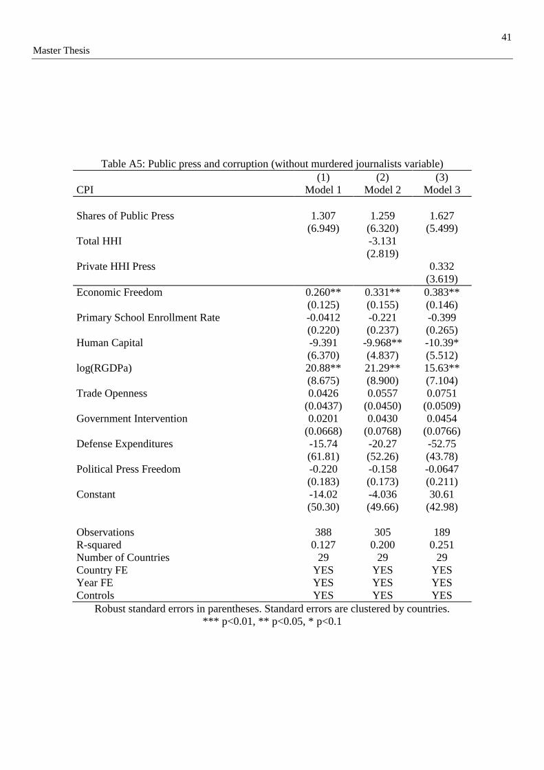
41

Master Thesis

Table A5: Public press and corruption (without murdered journalists variable)

(1) (2) (3)

CPI Model 1 Model 2 Model 3

Shares of Public Press 1.307 1.259 1.627

(6.949) (6.320) (5.499)

Total HHI -3.131

(2.819)

Private HHI Press 0.332

(3.619)

Economic Freedom 0.260** 0.331** 0.383**

(0.125) (0.155) (0.146)

Primary School Enrollment Rate -0.0412 -0.221 -0.399

(0.220) (0.237) (0.265)

Human Capital -9.391 -9.968** -10.39*

(6.370) (4.837) (5.512)

log(RGDPa) 20.88** 21.29** 15.63**

(8.675) (8.900) (7.104)

Trade Openness 0.0426 0.0557 0.0751

(0.0437) (0.0450) (0.0509)

Government Intervention 0.0201 0.0430 0.0454

(0.0668) (0.0768) (0.0766)

Defense Expenditures -15.74 -20.27 -52.75

(61.81) (52.26) (43.78)

Political Press Freedom -0.220 -0.158 -0.0647

(0.183) (0.173) (0.211)

Constant -14.02 -4.036 30.61

(50.30) (49.66) (42.98)

Observations 388 305 189

R-squared 0.127 0.200 0.251

Number of Countries 29 29 29

Country FE YES YES YES

Year FE YES YES YES

Controls YES YES YES

Robust standard errors in parentheses. Standard errors are clustered by countries.

*** p<0.01, ** p<0.05, * p<0.1

42

Master Thesis

Table A6: Public TV and corruption: quadratic impact (without murdered journalists variable)

(1) (2) (3) (4)

VARIABLES Model 1 Model 2 Model 3 Model 4

Shares of Public TV 20.64 22.21 35.56** 31.83*

(20.17) (19.95) (16.40) (15.99)

(Shares of Public TV)2 -8.735 -9.784 -20.05 -19.42

(17.57) (17.11) (13.30) (14.02)

Total HHI -0.257

(4.658)

Private HHI TV -8.684* -34.62***

(4.523) (11.53)

(Private HHI TV)2

24.65**

(10.43)

Economic Freedom 0.274** 0.274** 0.294** 0.281**

(0.102) (0.125) (0.128) (0.127)

Primary School Enrollment Rate -0.325 -0.405 -0.313 -0.334

(0.270) (0.288) (0.222) (0.206)

Human Capital -3.664 -3.666 -3.580 -2.672

(4.747) (5.220) (4.908) (4.917)

log(RGDPa) 26.83*** 26.35*** 29.09*** 30.02***

(7.912) (8.500) (8.168) (7.839)

Trade Openness 0.0272 0.0447 0.0351 0.0289

(0.0400) (0.0410) (0.0403) (0.0402)

Government Intervention 0.0466 0.0530 0.0528 0.0720

(0.0809) (0.0829) (0.0810) (0.0788)

Defense Expenditures 56.16 57.80 70.73 82.86*

(50.75) (55.51) (46.52) (44.89)

Political Press Freedom -0.135 -0.138 -0.160 -0.132

(0.143) (0.151) (0.179) (0.170)

Constant -48.00 -39.40 -61.12 -61.11

(44.13) (44.61) (37.96) (36.06)

Observations 216 203 191 191

R-squared 0.200 0.207 0.232 0.249

Number of Countries 29 29 29 29

Country FE YES YES YES YES

Year FE YES YES YES YES

Controls YES YES YES YES

Robust standard errors in parentheses. Standard errors are clustered by countries.

*** p<0.01, ** p<0.05, * p<0.1

43

Master Thesis

Table A7: Public Press and corruption: quadratic impact (without murdered journalists variable)

(1) (2) (3) (4)

VARIABLES Model 1 Model 2 Model 3 Model 4

Shares of Public Press 6.244 8.987 12.38 11.90*

(7.511) (8.377) (7.822) (6.613)

(Shares of Public Press)2 -10.42 -16.30* -22.15** -20.00***

(7.758) (8.094) (8.425) (6.637)

Total HHI -3.141

(2.824)

Private HHI Press -0.605 -6.237

(3.389) (20.18)

(Private HHI Press)2

5.381

(17.15)

Economic Freedom 0.261** 0.334** 0.385** 0.388**

(0.126) (0.157) (0.147) (0.148)

Primary School Enrollment Rate -0.0432 -0.225 -0.401 -0.405

(0.221) (0.240) (0.264) (0.265)

Human Capital -9.416 -10.02** -10.47* -10.52*

(6.381) (4.854) (5.537) (5.579)

log(RGDPa) 20.81** 21.15** 15.39** 15.24**

(8.702) (8.930) (7.108) (7.094)

Trade Openness 0.0429 0.0562 0.0756 0.0760

(0.0439) (0.0452) (0.0511) (0.0505)

Government Intervention 0.0202 0.0431 0.0444 0.0429

(0.0669) (0.0770) (0.0769) (0.0776)

Defense Expenditures -16.20 -21.20 -54.15 -54.18

(62.00) (52.54) (43.81) (44.26)

Political Press Freedom -0.218 -0.154 -0.0576 -0.0541

(0.183) (0.173) (0.211) (0.211)

Constant -13.11 -2.290 33.92 35.59

(50.57) (50.11) (43.21) (44.22)

Observations 388 305 189 189

R-squared 0.127 0.201 0.253 0.253

Number of Countries 29 29 29 29

Country FE YES YES YES YES

Year FE YES YES YES YES

Controls YES YES YES YES

Robust standard errors in parentheses. Standard errors are clustered by countries.

*** p<0.01, ** p<0.05, * p<0.1

44

Master Thesis

Table A8: Heterogeneous effects (without murdered journalists variable)

(1) (2) (3) (4) (5) (6) (7) (8) (9) (10)

VARIABLES Model 5 Model 5 Model 5 Model 5 Model 5 Model 5 Model 5 Model 5 Model 5 Model 5

Public TV Shares * Economic Freedom 0.163*

(0.0830) Public TV Shares * Log(RGDPa) 2.902**

(1.249)

Public TV Shares * Defense Expenditures 73.52 (53.56)

Public TV Shares * Human Capital 3.342

(1.978) Public TV Shares * Primary School Enrollment Rate 0.0776

(0.0462)

Public Press Shares * Economic Freedom 0.0748

(0.122) Public Press Shares * Log(RGDPa) 1.485

(1.373)

Public Press Shares * Defense Expenditures -6.146 (51.74)

Public Press Shares * Human Capital -0.570

(3.420) Public Press Shares * Primary School Enrollment Rate -0.0214

(0.0893)

Economic Freedom 0.297*** 0.282** 0.255** 0.271** 0.322*** 0.254** 0.247* 0.258**

(0.0965) (0.113) (0.106) (0.110) (0.109) (0.121) (0.123) (0.121) Log(RGDPa) 27.96*** 28.86*** 25.70*** 24.45*** 25.54*** 21.90** 18.26* 20.64**

(8.008) (7.834) (8.111) (8.030) (8.704) (8.955) (9.503) (8.784)

Defense Expenditures 67.66 -45.59 78.39 45.93 8.515 -89.95* 14.46 -17.15 (51.68) (44.26) (49.04) (49.69) (60.59) (48.01) (60.18) (61.57)

Human Capital -2.159 -1.943 -4.723 -5.357 -8.897 -7.343 -8.851 -9.247 (5.002) (4.900) (4.489) (4.111) (6.389) (6.438) (5.579) (6.435)

Primary School Enrollment Rate -0.319 -0.171 -0.289 -0.350 -0.00685 0.0182 -0.0378 -0.00556

(0.265) (0.253) (0.286) (0.262) (0.214) (0.235) (0.224) (0.238)

Trade Openness 0.0231 0.0631 0.0213 0.0143 0.0144 0.0328 0.0667 0.0417 0.0222 0.0422

(0.0401) (0.0401) (0.0387) (0.0413) (0.0341) (0.0436) (0.0408) (0.0428) (0.0473) (0.0431)

Government Intervention 0.0802 0.0500 0.0216 0.0408 0.0216 0.0774 0.0213 0.0198 0.00513 0.0199 (0.0743) (0.0764) (0.0771) (0.0716) (0.0768) (0.0559) (0.0695) (0.0671) (0.0657) (0.0669)

Political Press Freedom Index -0.137 0.0265 -0.162 -0.178 -0.0755 -0.230 -0.145 -0.219 -0.278 -0.220

(0.137) (0.130) (0.144) (0.131) (0.143) (0.197) (0.174) (0.187) (0.176) (0.179) Constant -40.47 49.30* -48.00 -47.47 -58.97 -25.56 62.94* -20.65 -31.73 -16.85

(41.49) (26.25) (47.18) (43.09) (41.91) (50.17) (32.05) (37.24) (46.92) (46.84)

Observations 216 216 216 216 216 388 388 388 388 388

R-squared 0.165 0.141 0.178 0.191 0.173 0.105 0.103 0.127 0.111 0.127

Number of Countries 29 29 29 29 29 29 29 29 29 29 Country FE YES YES YES YES YES YES YES YES YES YES

Year FE YES YES YES YES YES YES YES YES YES YES

Controls YES YES YES YES YES YES YES YES YES YES

Robust standard errors in parentheses. Standard errors are clustered by countries. *** p<0.01, ** p<0.05, * p<0.1

45

Master Thesis

Table A9: Additional heterogeneous effects

(1) (2) (3) (4) (5) (6)

CPI Model 5 Model 5 Model 5 Model 5 Model 5 Model 5

Public TV Shares * Trade Openness 0.106*

(0.0563)

Public TV Shares * Government Intervention 0.0590

(0.123)

Public TV Shares * Political Press Freedom 0.103

(0.179)

Public Press Shares * Trade Openness -0.0443

(0.0516)

Public Press Shares * Government Intervention 0.106

(0.0716)

Public Press Shares * Political Press Freedom 0.269

(0.162)

Trade Openness 0.0155 0.0278 0.0392 0.0468

(0.0356) (0.0399) (0.0428) (0.0447)

Government Intervention 0.0475 0.0398 0.0201 0.0252

(0.0751) (0.0835) (0.0668) (0.0675)

Political Press Freedom -0.133 -0.187 -0.233 -0.225

(0.141) (0.154) (0.183) (0.179)

Economic Freedom 0.261** 0.263** 0.254** 0.238* 0.274** 0.271**

(0.101) (0.117) (0.111) (0.124) (0.107) (0.122)

Murdered Journalists 0.605 0.732 0.505 0.486 0.485 0.368

(0.718) (0.766) (0.833) (0.513) (0.480) (0.497)

Primary School Enrollment Rate -0.297 -0.285 -0.209 -0.0305 -0.0372 0.0381

(0.238) (0.272) (0.263) (0.221) (0.212) (0.207)

Human Capital -4.461 -4.481 -6.050 -8.026 -8.953 -10.03

(4.787) (4.635) (4.582) (6.897) (6.358) (6.298)

Log(RGDPa) 26.13*** 29.46*** 23.10*** 24.95** 22.70** 15.72*

(8.093) (8.366) (8.042) (9.157) (8.941) (8.744)

Defense Expenditures 65.31 64.68 48.06 -2.955 -9.059 -11.85

(53.26) (51.22) (49.06) (61.59) (67.11) (64.34)

Constant -40.48 -52.08 -30.71 -33.05 -24.48 -1.693

(44.11) (47.78) (47.38) (50.62) (55.19) (52.95)

Observations 216 216 216 388 388 388

R-squared 0.209 0.182 0.172 0.124 0.130 0.122

Number of Countries 29 29 29 29 29 29

Country FE YES YES YES YES YES YES

Year FE YES YES YES YES YES YES

Controls YES YES YES YES YES YES

Robust standard errors in parentheses. Standard errors are clustered by countries.

*** p<0.01, ** p<0.05, * p<0.1

46

Master Thesis

Table A10: Additional heterogeneous effects (without murdered journalists variable)

(1) (2) (3) (4) (5) (6)

VARIABLES Model 5 Model 5 Model 5 Model 5 Model 5 Model 5

Public TV Shares * Trade Openness 0.111*

(0.0575)

Public TV Shares * Government Intervention 0.0577

(0.125)

Public TV Shares * Political Press Freedom 0.106

(0.179)

Public Press Shares * Trade Openness -0.0445

(0.0536)

Public Press Shares * Government Intervention 0.0997

(0.0752)

Public Press Shares * Political Press Freedom 0.267

(0.166)

Trade Openness 0.0212 0.0307 0.0412 0.0482

(0.0371) (0.0404) (0.0434) (0.0452)

Government Intervention 0.0449 0.0364 0.0204 0.0254

(0.0750) (0.0826) (0.0670) (0.0676)

Political Press Freedom -0.105 -0.151 -0.231 -0.223

(0.135) (0.144) (0.184) (0.180)

Economic Freedom 0.275*** 0.277** 0.267** 0.243* 0.281** 0.275**

(0.0987) (0.116) (0.108) (0.123) (0.107) (0.120)

Primary School Enrollment Rate -0.302 -0.295 -0.224 -0.0350 -0.0420 0.0339

(0.248) (0.286) (0.274) (0.224) (0.213) (0.210)

Human Capital -4.475 -4.667 -5.941 -8.312 -9.276 -10.28

(4.802) (4.709) (4.589) (6.819) (6.275) (6.204)

Log(RGDPa) 24.81*** 27.77*** 22.44*** 24.55** 22.10** 15.37*

(7.847) (8.176) (8.072) (9.080) (8.825) (8.627)

Defense Expenditures 60.03 57.45 45.20 -6.760 -13.29 -15.04

(53.08) (51.41) (49.37) (60.44) (65.58) (62.91)

Constant -35.17 -44.38 -27.27 -30.12 -20.73 0.848

(44.41) (48.59) (48.39) (50.05) (54.45) (52.29)

Observations 216 216 216 388 388 388

R-squared 0.204 0.176 0.169 0.123 0.129 0.122

Number of Countries 29 29 29 29 29 29

Country FE YES YES YES YES YES YES

Year FE YES YES YES YES YES YES

Controls YES YES YES YES YES YES

Robust standard errors in parentheses. Standard errors are clustered by countries.

*** p<0.01, ** p<0.05, * p<0.1

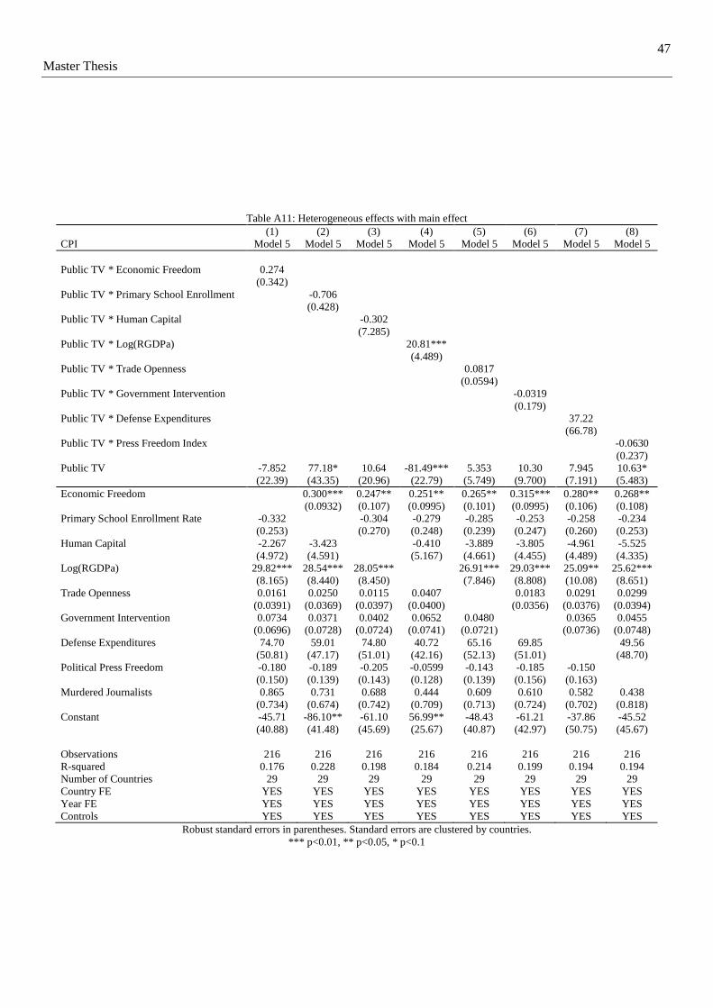
47

Master Thesis

Table A11: Heterogeneous effects with main effect

(1) (2) (3) (4) (5) (6) (7) (8)

CPI Model 5 Model 5 Model 5 Model 5 Model 5 Model 5 Model 5 Model 5

Public TV * Economic Freedom 0.274

(0.342)

Public TV * Primary School Enrollment -0.706

(0.428)

Public TV * Human Capital -0.302

(7.285)

Public TV * Log(RGDPa) 20.81***

(4.489)

Public TV * Trade Openness 0.0817

(0.0594)

Public TV * Government Intervention -0.0319

(0.179)

Public TV * Defense Expenditures 37.22

(66.78)

Public TV * Press Freedom Index -0.0630

(0.237)

Public TV -7.852 77.18* 10.64 -81.49*** 5.353 10.30 7.945 10.63*

(22.39) (43.35) (20.96) (22.79) (5.749) (9.700) (7.191) (5.483)

Economic Freedom 0.300*** 0.247** 0.251** 0.265** 0.315*** 0.280** 0.268**

(0.0932) (0.107) (0.0995) (0.101) (0.0995) (0.106) (0.108)

Primary School Enrollment Rate -0.332 -0.304 -0.279 -0.285 -0.253 -0.258 -0.234

(0.253) (0.270) (0.248) (0.239) (0.247) (0.260) (0.253)

Human Capital -2.267 -3.423 -0.410 -3.889 -3.805 -4.961 -5.525

(4.972) (4.591) (5.167) (4.661) (4.455) (4.489) (4.335)

Log(RGDPa) 29.82*** 28.54*** 28.05*** 26.91*** 29.03*** 25.09** 25.62***

(8.165) (8.440) (8.450) (7.846) (8.808) (10.08) (8.651)

Trade Openness 0.0161 0.0250 0.0115 0.0407 0.0183 0.0291 0.0299

(0.0391) (0.0369) (0.0397) (0.0400) (0.0356) (0.0376) (0.0394)

Government Intervention 0.0734 0.0371 0.0402 0.0652 0.0480 0.0365 0.0455

(0.0696) (0.0728) (0.0724) (0.0741) (0.0721) (0.0736) (0.0748)

Defense Expenditures 74.70 59.01 74.80 40.72 65.16 69.85 49.56

(50.81) (47.17) (51.01) (42.16) (52.13) (51.01) (48.70)

Political Press Freedom -0.180 -0.189 -0.205 -0.0599 -0.143 -0.185 -0.150

(0.150) (0.139) (0.143) (0.128) (0.139) (0.156) (0.163)

Murdered Journalists 0.865 0.731 0.688 0.444 0.609 0.610 0.582 0.438

(0.734) (0.674) (0.742) (0.709) (0.713) (0.724) (0.702) (0.818)

Constant -45.71 -86.10** -61.10 56.99** -48.43 -61.21 -37.86 -45.52

(40.88) (41.48) (45.69) (25.67) (40.87) (42.97) (50.75) (45.67)

Observations 216 216 216 216 216 216 216 216

R-squared 0.176 0.228 0.198 0.184 0.214 0.199 0.194 0.194

Number of Countries 29 29 29 29 29 29 29 29

Country FE YES YES YES YES YES YES YES YES

Year FE YES YES YES YES YES YES YES YES

Controls YES YES YES YES YES YES YES YES

Robust standard errors in parentheses. Standard errors are clustered by countries.

*** p<0.01, ** p<0.05, * p<0.1

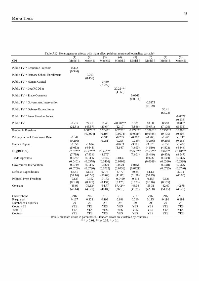
48

Master Thesis

Table A12: Heterogeneous effects with main effect (without murdered journalists variable)

(1) (2) (3) (4) (5) (6) (7) (8)

CPI Model 5 Model 5 Model 5 Model 5 Model 5 Model 5 Model 5 Model 5

Public TV * Economic Freedom 0.302

(0.346)

Public TV * Primary School Enrollment -0.703

(0.450)

Public TV * Human Capital -0.480

(7.222)

Public TV * Log(RGDPa) 20.22***

(4.363)

Public TV * Trade Openness 0.0868

(0.0614)

Public TV * Government Intervention -0.0375

(0.179)

Public TV * Defense Expenditures 30.41

(66.23)

Public TV * Press Freedom Index -0.0627

(0.238)

Public TV -9.217 77.25 11.46 -78.70*** 5.321 10.80 8.568 10.80*

(22.81) (45.57) (20.64) (22.17) (5.866) (9.671) (7.109) (5.535)

Economic Freedom 0.317*** 0.264** 0.262** 0.279*** 0.329*** 0.293*** 0.279**

(0.0924) (0.105) (0.0971) (0.0984) (0.0988) (0.105) (0.106)

Primary School Enrollment Rate -0.347 -0.311 -0.285 -0.290 -0.260 -0.265 -0.247

(0.266) (0.281) (0.255) (0.249) (0.256) (0.269) (0.264)

Human Capital -2.356 -3.634 -0.633 -3.907 -3.926 -5.059 -5.422

(5.033) (4.648) (5.147) (4.693) (4.510) (4.502) (4.344)

Log(RGDPa) 27.87*** 26.77*** 26.46*** 25.58*** 27.63*** 23.66** 25.10***

(7.799) (7.934) (8.276) (7.601) (8.449) (9.879) (8.647)

Trade Openness 0.0227 0.0306 0.0166 0.0435 0.0232 0.0338 0.0325

(0.0401) (0.0378) (0.0406) (0.0409) (0.0369) (0.0390) (0.0398)

Government Intervention 0.0719 0.0335 0.0370 0.0624 0.0454 0.0348 0.0426

(0.0700) (0.0730) (0.0722) (0.0736) (0.0721) (0.0735) (0.0740)

Defense Expenditures 66.41 51.15 67.74 37.77 59.84 64.13 47.11

(51.16) (46.56) (50.62) (41.86) (51.98) (50.79) (48.90)

Political Press Freedom -0.139 -0.152 -0.173 -0.0429 -0.114 -0.155 -0.121

(0.138) (0.129) (0.134) (0.125) (0.133) (0.146) (0.155)

Constant -35.93 -79.13* -54.77 57.42** -43.04 -55.31 -32.07 -42.78

(40.14) (40.27) (46.04) (26.13) (41.31) (42.58) (51.15) (46.28)

Observations 216 216 216 216 216 216 216 216

R-squared 0.167 0.222 0.193 0.181 0.210 0.195 0.190 0.192

Number of Countries 29 29 29 29 29 29 29 29

Country FE YES YES YES YES YES YES YES YES

Year FE YES YES YES YES YES YES YES YES

Controls YES YES YES YES YES YES YES YES

Robust standard errors in parentheses. Standard errors are clustered by countries.

*** p<0.01, ** p<0.05, * p<0.1

49

Master Thesis

Table A13: Public TV delayed effect / lagged variables (without murdered journalists variable)

(1) (2) (3) (4) (5) (6) (7) (8)

CPI Model 7 Model 7 Model 7 Model 7 Model 7 Model 7 Model 7 Model 7

Public TVt-1 41.45** 49.49*** 49.71*** 41.22**

(17.30) (14.31) (11.67) (16.74)

(Public TVt-1)2 -30.21** -36.53*** -38.62*** -29.91**

(14.29) (10.96) (9.919) (13.62)

Private TV HHIt-1 -4.688 -30.24**

(4.331) (14.27)

(Private TV HHIt-1)2 23.21*

(12.86)

Total HHIt-1 -0.105

(4.039)

Public TVt-2 14.66 22.08 20.03 14.98

(18.15) (17.48) (15.53) (17.73)

(Public TVt-2)2 -10.24 -15.74 -16.27 -10.93

(14.39) (12.28) (12.04) (13.74)

Private TV HHIt-2 -3.598 -27.30

(6.310) (21.00)

(Private TV HHIt-2)2 21.24

(17.62)

Total HHIt-2 1.335

(3.485)

Economic Freedom 0.219** 0.218 0.228 0.271* 0.103 0.146 0.160 0.103

(0.103) (0.151) (0.152) (0.133) (0.171) (0.207) (0.202) (0.183)

Primary School Enrollment -0.326 -0.308 -0.349* -0.385 -0.0492 -0.135 -0.243 -0.0885

(0.210) (0.197) (0.187) (0.231) (0.195) (0.202) (0.200) (0.191)

Human Capital -8.637* -9.383* -7.845 -9.317* -4.648 -3.758 -1.696 -3.945

(4.675) (4.798) (5.104) (4.763) (4.762) (4.927) (5.144) (4.943)

log(RGDPa) 16.36** 15.38** 16.96*** 16.90** 17.82** 20.20*** 22.12*** 17.54**

(6.882) (6.891) (6.086) (7.024) (7.456) (6.907) (6.031) (6.980)

Trade Openness 0.0176 0.0266 0.0221 0.0348 0.0259 0.0287 0.0229 0.0358

(0.0399) (0.0410) (0.0393) (0.0406) (0.0393) (0.0372) (0.0343) (0.0364)

Government Intervention 0.00390 0.00947 0.0264 -0.00385 -0.0173 -0.0332 -0.0171 -0.00851

(0.0481) (0.0509) (0.0534) (0.0514) (0.0481) (0.0537) (0.0620) (0.0548)

Defense Expenditures -36.47 -38.48 -24.77 -28.03 14.74 44.72 64.13** 17.53

(43.84) (46.92) (39.68) (48.36) (47.81) (41.40) (31.21) (47.07)

Political Press Freedom -0.185 -0.160 -0.176 -0.250 -0.135 -0.136 -0.173 -0.156

(0.156) (0.198) (0.185) (0.157) (0.172) (0.194) (0.193) (0.170)

Constant 22.76 26.84 22.49 25.43 -12.57 -20.49 -21.21 -10.04

(41.15) (38.33) (32.87) (39.28) (33.64) (32.85) (30.87) (33.56)

Observations 216 190 190 203 205 179 179 193

R-squared 0.191 0.202 0.228 0.202 0.095 0.109 0.129 0.094

Number of Countries 29 29 29 29 29 29 29 29

Country FE YES YES YES YES YES YES YES YES

Year FE YES YES YES YES YES YES YES YES

Controls YES YES YES YES YES YES YES YES

Robust standard errors in parentheses. Standard errors are clustered by countries.

*** p<0.01, ** p<0.05, * p<0.1

50

Master Thesis

Table A14: Public press delayed effect / lagged variables (without murdered journalists)

(1) (2) (3) (4) (5) (6) (7) (8)

CPI Model 7 Model 7 Model 7 Model 7 Model 7 Model 7 Model 7 Model 7

Public Presst-1 14.58*** 32.71*** 20.85** 14.79***

(3.554) (10.67) (7.792) (4.005)

(Public Presst-1)2 -5.442 -36.08* -9.344 -7.167

(9.041) (17.86) (16.19) (8.003)

Private Press HHIt-1 -5.108 -35.98*

(3.092) (20.53)

(Private Press HHIt-1)2 30.37

(18.56)

Total HHIt-1 -1.996

(1.835)

Public Presst-2 32.15** 26.76 18.76 27.95**

(12.60) (17.96) (18.00) (12.66)

(Public Presst-2)2 -20.61 -13.51 5.201 -15.00

(19.71) (29.40) (34.96) (19.28)

Private Press HHIt-2 1.658 -22.01

(3.987) (22.82)

(Private Press HHIt-2)2 22.65

(19.15)

Total HHIt-2 -0.0329

(1.121)

Economic Freedom 0.211* 0.166 0.154 0.216 0.166 0.155 0.129 0.166

(0.110) (0.144) (0.128) (0.141) (0.105) (0.168) (0.158) (0.167)

Primary School Enrollment -0.0762 -0.356 -0.379 -0.173 -0.0779 -0.267 -0.259 -0.104

(0.213) (0.285) (0.279) (0.249) (0.236) (0.303) (0.284) (0.265)

Human Capital -13.72** -15.24** -16.11** -14.40** -15.26** -8.923 -9.551 -13.57**

(5.950) (6.626) (6.857) (5.478) (5.756) (6.610) (6.767) (5.747)

log(RGDPa) 18.79** 15.14* 13.16 18.38** 17.05* 11.94 11.23 15.19*

(8.145) (8.812) (8.610) (8.678) (8.723) (8.614) (8.274) (8.414)

Trade Openness 0.0293 0.0291 0.0398 0.0269 0.0218 0.0550 0.0555 0.0228

(0.0338) (0.0382) (0.0369) (0.0359) (0.0321) (0.0445) (0.0451) (0.0362)

Government Intervention -0.00479 0.0347 0.0415 0.0469 -0.0638 -0.0570 -0.0469 -0.0291

(0.0587) (0.0423) (0.0451) (0.0506) (0.0456) (0.0446) (0.0453) (0.0541)

Defense Expenditures -18.75 -60.61 -70.64 -32.24 -32.69 -32.50 -37.13 -44.47

(56.10) (66.04) (68.44) (59.24) (59.74) (71.06) (69.84) (59.38)

Political Press Freedom -0.0950 -0.0792 -0.0377 -0.0896 -0.0428 -0.0614 -0.0324 -0.0528

(0.150) (0.197) (0.193) (0.163) (0.156) (0.181) (0.181) (0.175)

Constant 15.16 63.15 78.77 25.52 33.86 47.43 54.59 36.59

(44.52) (52.94) (52.47) (48.32) (48.23) (57.91) (56.09) (50.12)

Observations 387 187 187 304 379 178 178 297

R-squared 0.115 0.195 0.215 0.163 0.130 0.156 0.164 0.131

Number of Countries 29 29 29 29 29 29 29 29

Country FE YES YES YES YES YES YES YES YES

Year FE YES YES YES YES YES YES YES YES

Controls YES YES YES YES YES YES YES YES

Robust standard errors in parentheses. Standard errors are clustered by countries.

*** p<0.01, ** p<0.05, * p<0.1

51

Master Thesis

Table A15: Heterogeneous trends (without the murdered journalist variable)

(1) (2) (3) (4) (5) (6) (7) (8)

VARIABLES Model 6 Model 6 Model 6 Model 6 Model 6 Model 6 Model 6 Model 6

Public TV * Pre-2002 1.100 1.112 1.039 1.040

(1.532) (1.440) (1.442) (1.461)

Public TV * Post-2002 2.281 2.253 2.665* 1.976

(1.440) (1.398) (1.364) (1.462)

Total HHI 1.959 2.371

(4.350) (4.665)

Private HHI TV -4.237 -35.84** -5.483 -33.22**

(5.560) (13.00) (5.834) (14.12)

(Private HHI TV)2

29.71** 26.33**

(10.86) (12.14)

Economic Freedom 0.293*** 0.322** 0.317** 0.311** 0.272** 0.305** 0.299** 0.295**

(0.100) (0.125) (0.130) (0.129) (0.103) (0.129) (0.130) (0.127)

Primary School Enrollment Rate -0.144 -0.221 -0.144 -0.159 -0.168 -0.244 -0.144 -0.160

(0.266) (0.267) (0.223) (0.211) (0.282) (0.280) (0.215) (0.207)

Human Capital -2.242 -2.215 -2.660 -1.391 -3.271 -3.235 -4.017 -2.656

(5.218) (5.623) (5.374) (5.141) (5.259) (5.679) (5.436) (5.272)

log(RGDPa) 0.0625 0.0826** 0.0767* 0.0736* 0.0426 0.0636 0.0543 0.0554

(0.0381) (0.0390) (0.0375) (0.0376) (0.0388) (0.0406) (0.0385) (0.0391)

Trade Openness 0.0361 0.0382 0.0310 0.0584 0.0274 0.0290 0.0202 0.0470

(0.0884) (0.0921) (0.0945) (0.0879) (0.0856) (0.0893) (0.0909) (0.0865)

Government Intervention -63.31 -61.62 -56.32 -48.00 -41.27 -39.80 -33.92 -30.45

(56.88) (58.08) (61.00) (62.41) (52.15) (53.79) (56.07) (57.38)

Defense Expenditures 0.0467 0.0526 0.0631 0.106 -0.00274 0.000634 -0.00664 0.0453

(0.143) (0.148) (0.162) (0.149) (0.123) (0.127) (0.143) (0.139)

Constant 54.51* 59.22** 56.08** 56.87** 61.73** 65.72** 62.51** 62.44**

(28.05) (28.14) (25.68) (23.91) (29.44) (28.69) (24.50) (23.09)

Observations 216 203 191 191 216 203 191 191

R-squared 0.103 0.113 0.109 0.137 0.111 0.121 0.121 0.142

Number of Countries 29 29 29 29 29 29 29 29

Country FE YES YES YES YES YES YES YES YES

Year FE YES YES YES YES YES YES YES YES

Controls YES YES YES YES YES YES YES YES

Robust standard errors in parentheses. Standard errors are clustered by countries.

*** p<0.01, ** p<0.05, * p<0.1

52

Master Thesis

*

Table A16: Public TV and corruption relationship: exclusion of outliers

(1) (2) (3) (4) (5) (6) (7) (8)

CPI Model 1 Model 2 Model 3 Model 4 Model 1 Model 2 Model 3 Model 4

Shares of Public TV 4.138 3.094 4.413 3.994 12.58 16.49 27.06* 26.51* (5.610) (5.255) (4.735) (4.555) (18.17) (17.00) (15.26) (14.84) (Shares of Public TV)

2 -6.880 -11.14 -18.25 -18.09

(16.13) (14.04) (11.84) (11.82) Total HHI 2.952 3.642 (4.128) (4.099) Private HHI TV -6.548* -11.20 -8.610** -12.42 (3.792) (12.42) (3.510) (11.58) (Private HHI TV)

2 4.430 3.648

(12.57) (10.95)

Economic Freedom 0.246** 0.243* 0.245* 0.242* 0.244** 0.238* 0.252* 0.249* (0.0986) (0.133) (0.125) (0.127) (0.0975) (0.132) (0.126) (0.128) Murdered Journalists 0.539 1.090* 1.371*** 1.370*** 0.523 1.100* 1.240*** 1.240*** (0.628) (0.562) (0.409) (0.415) (0.641) (0.568) (0.430) (0.435) Primary School Enrollment Rate -0.211 -0.279 -0.190 -0.195 -0.239 -0.323 -0.239 -0.243 (0.248) (0.235) (0.189) (0.189) (0.244) (0.242) (0.199) (0.200) Human Capital -8.742 -8.218 -8.668 -8.423 -8.342 -7.579 -7.869 -7.674 (5.961) (6.413) (6.062) (6.229) (5.988) (6.605) (6.272) (6.453) log(RGDPa) 28.60*** 28.40*** 32.66*** 32.82*** 28.28*** 27.74*** 32.00*** 32.14*** (8.243) (8.590) (8.628) (8.500) (8.173) (8.623) (8.737) (8.624) Trade Openness 0.0116 0.0293 0.0166 0.0157 0.0107 0.0290 0.0141 0.0134 (0.0328) (0.0354) (0.0338) (0.0343) (0.0340) (0.0365) (0.0354) (0.0359) Government Intervention -0.0166 -0.00941 -0.0170 -0.0123 -0.0102 0.00142 -0.000353 0.00337 (0.0627) (0.0664) (0.0676) (0.0688) (0.0663) (0.0690) (0.0683) (0.0716) Defense Expenditures 44.97 45.13 70.27 72.68 43.69 41.59 66.13 68.15 (49.30) (52.20) (44.90) (44.37) (49.45) (52.21) (46.05) (45.65) Political Press Freedom -0.184 -0.193 -0.231 -0.226 -0.181 -0.182 -0.225 -0.221 (0.151) (0.172) (0.187) (0.188) (0.151) (0.172) (0.185) (0.185)

Constant -39.62 -34.73 -57.09 -57.29 -38.33 -32.54 -56.76 -56.92

(46.21) (45.55) (41.53) (41.12) (46.39) (46.24) (42.27) (41.93)

Observations 211 198 186 186 211 198 186 186

R-squared 0.204 0.220 0.253 0.254 0.206 0.225 0.265 0.265

Number of Countries 29 29 29 29 29 29 29 29

Country FE YES YES YES YES YES YES YES YES

Year FE YES YES YES YES YES YES YES YES

Controls YES YES YES YES YES YES YES YES

Robust standard errors in parentheses. Standard errors are clustered by countries.

*** p<0.01, ** p<0.05, * p<0.1

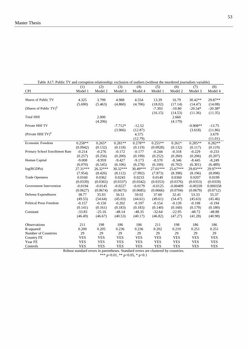
53

Master Thesis

Table A17: Public TV and corruption relationship: exclusion of outliers (without the murdered journalists variable)

(1) (2) (3) (4) (5) (6) (7) (8)

CPI Model 1 Model 2 Model 3 Model 4 Model 1 Model 2 Model 3 Model 4

Shares of Public TV 4.325 3.799 4.988 4.554 13.39 16.79 30.42** 29.87** (5.690) (5.463) (4.860) (4.706) (18.02) (17.14) (14.47) (14.08) (Shares of Public TV)

2 -7.393 -10.80 -20.54* -20.38*

(16.15) (14.53) (11.36) (11.35) Total HHI 2.000 2.660 (4.206) (4.179) Private HHI TV -7.712* -12.52 -9.908** -13.75 (3.966) (12.87) (3.618) (11.86) (Private HHI TV)

2 4.575 3.679

(12.79) (11.01)

Economic Freedom 0.258** 0.265* 0.281** 0.278** 0.255** 0.261* 0.285** 0.282** (0.0942) (0.132) (0.118) (0.119) (0.0928) (0.132) (0.117) (0.119) Primary School Enrollment Rate -0.214 -0.276 -0.172 -0.177 -0.244 -0.318 -0.229 -0.233 (0.257) (0.256) (0.200) (0.199) (0.252) (0.260) (0.206) (0.207) Human Capital -9.008 -8.959 -9.427 -9.173 -8.570 -8.346 -8.445 -8.249 (6.070) (6.545) (6.106) (6.278) (6.100) (6.702) (6.301) (6.489) log(RGDPa) 27.31*** 26.32*** 30.32*** 30.49*** 27.01*** 25.67*** 29.83*** 29.97*** (7.954) (8.426) (8.112) (7.992) (7.873) (8.398) (8.196) (8.098) Trade Openness 0.0160 0.0362 0.0243 0.0233 0.0149 0.0360 0.0207 0.0199 (0.0339) (0.0365) (0.0337) (0.0342) (0.0353) (0.0376) (0.0353) (0.0359) Government Intervention -0.0194 -0.0145 -0.0227 -0.0179 -0.0125 -0.00409 -0.00339 0.000358 (0.0627) (0.0674) (0.0675) (0.0685) (0.0666) (0.0704) (0.0679) (0.0712) Defense Expenditures 38.77 35.93 56.51 59.02 37.60 32.41 53.33 55.37 (49.55) (54.64) (45.03) (44.61) (49.61) (54.47) (45.63) (45.46) Political Press Freedom -0.157 -0.150 -0.202 -0.197 -0.154 -0.139 -0.198 -0.194 (0.141) (0.161) (0.183) (0.183) (0.140) (0.160) (0.179) (0.180)

Constant -33.83 -25.16 -48.14 -48.35 -32.64 -22.95 -48.72 -48.88

(46.49) (46.67) (40.53) (40.17) (46.82) (47.27) (41.28) (40.98)

Observations 211 198 186 186 211 198 186 186

R-squared 0.200 0.205 0.236 0.236 0.202 0.210 0.251 0.251

Number of Countries 29 29 29 29 29 29 29 29

Country FE YES YES YES YES YES YES YES YES

Year FE YES YES YES YES YES YES YES YES

Controls YES YES YES YES YES YES YES YES

Robust standard errors in parentheses. Standard errors are clustered by countries.

*** p<0.01, ** p<0.05, * p<0.1

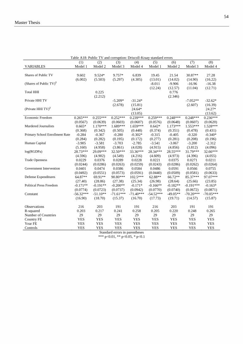
54

Master Thesis

Table A18: Public TV and corruption: Driscoll-Kraay standard errors

(1) (2) (3) (4) (5) (6) (7) (8)

VARIABLES Model 1 Model 2 Model 3 Model 4 Model 1 Model 2 Model 3 Model 4

Shares of Public TV 9.602 9.524* 9.757* 6.839 19.45 21.54 30.87** 27.28 (6.002) (5.503) (5.297) (4.305) (13.01) (14.02) (14.90) (16.22) (Shares of Public TV)

2 -8.011 -9.906 -16.96 -16.38

(12.24) (12.57) (11.04) (12.71) Total HHI 0.225 0.776 (2.212) (2.346) Private HHI TV -5.209* -31.24* -7.052** -32.62* (2.678) (15.81) (2.607) (16.39) (Private HHI TV)

2 24.64* 24.27*

(13.05) (13.62)

Economic Freedom 0.265*** 0.255*** 0.252*** 0.239*** 0.259*** 0.248*** 0.248*** 0.236*** (0.0567) (0.0639) (0.0603) (0.0607) (0.0576) (0.0648) (0.0607) (0.0620) Murdered Journalists 0.665* 1.170*** 1.689*** 1.659*** 0.642* 1.173*** 1.553*** 1.528*** (0.368) (0.342) (0.505) (0.448) (0.374) (0.351) (0.478) (0.431) Primary School Enrollment Rate -0.284 -0.367 -0.280 -0.302* -0.315 -0.405 -0.320 -0.340* (0.284) (0.282) (0.195) (0.172) (0.277) (0.281) (0.208) (0.196) Human Capital -3.905 -3.581 -3.703 -2.785 -3.541 -3.067 -3.200 -2.312 (5.160) (4.958) (3.861) (4.028) (4.915) (4.856) (3.812) (4.096) log(RGDPa) 28.73*** 29.09*** 32.50*** 33.36*** 28.34*** 28.55*** 31.79*** 32.66*** (4.596) (4.902) (4.549) (4.216) (4.609) (4.973) (4.396) (4.055) Trade Openness 0.0229 0.0376 0.0289 0.0228 0.0221 0.0375 0.0271 0.0211 (0.0244) (0.0286) (0.0263) (0.0259) (0.0243) (0.0286) (0.0262) (0.0264) Government Intervention 0.0401 0.0474 0.0386 0.0584 0.0486 0.0591 0.0566 0.0755 (0.0492) (0.0551) (0.0573) (0.0591) (0.0440) (0.0509) (0.0581) (0.0633) Defense Expenditures 64.87** 69.91** 90.80*** 102.5*** 62.88** 66.72** 85.37*** 97.07*** (27.40) (28.86) (27.38) (25.34) (26.98) (28.64) (25.66) (23.85) Political Press Freedom -0.171** -0.191** -0.200** -0.171* -0.166** -0.182** -0.191*** -0.163* (0.0774) (0.0723) (0.0737) (0.0942) (0.0770) (0.0740) (0.0672) (0.0871)

Constant -56.32*** -51.10** -71.61*** -71.40*** -54.52*** -49.05** -70.20*** -70.05***

(16.90) (18.70) (15.37) (16.70) (17.73) (19.71) (14.57) (15.87)

Observations 216 203 191 191 216 203 191 191

R-squared 0.203 0.217 0.241 0.258 0.205 0.220 0.248 0.265

Number of Countries 29 29 29 29 29 29 29 29

Country FE YES YES YES YES YES YES YES YES

Year FE YES YES YES YES YES YES YES YES

Controls YES YES YES YES YES YES YES YES

Standard errors in parentheses

*** p<0.01, ** p<0.05, * p<0.1

55

Master Thesis

Table A19: Public TV and corruption: Driscoll-Kraay standard errors (without the murdered journalists variable)

(1) (2) (3) (4) (5) (6) (7) (8)

VARIABLES Model 1 Model 2 Model 3 Model 4 Model 1 Model 2 Model 3 Model 4

Shares of Public TV 9.911 10.34* 10.67* 7.675* 20.64 22.21 35.56** 31.83* (6.087) (5.912) (5.645) (4.434) (12.90) (13.82) (15.36) (16.10) (Shares of Public TV)

2 -8.735 -9.784 -20.05* -19.42

(12.38) (12.95) (11.11) (12.53) Total HHI -0.799 -0.257 (2.021) (2.181) Private HHI TV -6.640** -33.16* -8.684*** -34.62* (3.001) (16.61) (3.086) (17.22) (Private HHI TV)

2 25.14* 24.65*

(13.40) (13.96)

Economic Freedom 0.281*** 0.281*** 0.304*** 0.290*** 0.274*** 0.274*** 0.294*** 0.281*** (0.0568) (0.0670) (0.0669) (0.0651) (0.0574) (0.0670) (0.0658) (0.0655) Primary School Enrollment Rate -0.292 -0.366 -0.265 -0.287 -0.325 -0.405 -0.313 -0.334 (0.289) (0.297) (0.206) (0.181) (0.280) (0.290) (0.218) (0.205) Human Capital -4.066 -4.172 -4.225 -3.278 -3.664 -3.666 -3.580 -2.672 (5.286) (5.130) (4.088) (4.236) (5.000) (4.920) (3.966) (4.251) log(RGDPa) 27.20*** 26.90*** 29.67*** 30.59*** 26.83*** 26.35*** 29.09*** 30.02*** (4.493) (5.254) (4.694) (4.328) (4.460) (5.339) (4.406) (4.088) Trade Openness 0.0283 0.0447 0.0382 0.0318 0.0272 0.0447 0.0351 0.0289 (0.0260) (0.0306) (0.0299) (0.0291) (0.0258) (0.0305) (0.0290) (0.0290) Government Intervention 0.0372 0.0415 0.0307 0.0511 0.0466 0.0530 0.0528 0.0720 (0.0501) (0.0546) (0.0564) (0.0580) (0.0447) (0.0492) (0.0576) (0.0630) Defense Expenditures 58.07** 60.97* 75.72** 87.93*** 56.16* 57.80* 70.73** 82.86*** (28.20) (30.75) (29.89) (26.93) (27.53) (30.79) (27.57) (25.24) Political Press Freedom -0.139* -0.148** -0.168** -0.139 -0.135* -0.138* -0.160** -0.132 (0.0713) (0.0717) (0.0696) (0.0889) (0.0710) (0.0747) (0.0627) (0.0809)

Constant -49.72*** -41.44** -61.86*** -61.83*** -48.00** -39.40* -61.12*** -61.11***

(16.81) (20.17) (16.03) (17.68) (17.49) (21.09) (14.68) (16.42)

Observations 216 203 191 191 216 203 191 191

R-squared 0.198 0.205 0.222 0.239 0.200 0.207 0.232 0.249

Number of Countries 29 29 29 29 29 29 29 29

Country FE YES YES YES YES YES YES YES YES

Year FE YES YES YES YES YES YES YES YES

Controls YES YES YES YES YES YES YES YES

Standard errors in parentheses

*** p<0.01, ** p<0.05, * p<0.1

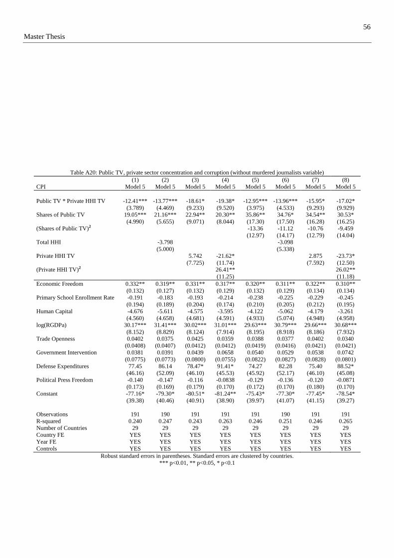
56

Master Thesis

Table A20: Public TV, private sector concentration and corruption (without murdered journalists variable)

(1) (2) (3) (4) (5) (6) (7) (8)

CPI Model 5 Model 5 Model 5 Model 5 Model 5 Model 5 Model 5 Model 5

Public TV * Private HHI TV -12.41*** -13.77*** -18.61* -19.38* -12.95*** -13.96*** -15.95* -17.02*

(3.789) (4.469) (9.233) (9.520) (3.975) (4.533) (9.293) (9.929)

Shares of Public TV 19.05*** 21.16*** 22.94** 20.30** 35.86** 34.76* 34.54** 30.53*

(4.990) (5.655) (9.071) (8.044) (17.30) (17.50) (16.28) (16.25)

(Shares of Public TV)2 -13.36 -11.12 -10.76 -9.459

(12.97) (14.17) (12.79) (14.04)

Total HHI -3.798 -3.098

(5.000) (5.338)

Private HHI TV 5.742 -21.62* 2.875 -23.73*

(7.725) (11.74) (7.592) (12.50)

(Private HHI TV)2 26.41** 26.02**

(11.25) (11.18)

Economic Freedom 0.332** 0.319** 0.331** 0.317** 0.320** 0.311** 0.322** 0.310**

(0.132) (0.127) (0.132) (0.129) (0.132) (0.129) (0.134) (0.134)

Primary School Enrollment Rate -0.191 -0.183 -0.193 -0.214 -0.238 -0.225 -0.229 -0.245

(0.194) (0.189) (0.204) (0.174) (0.210) (0.205) (0.212) (0.195)

Human Capital -4.676 -5.611 -4.575 -3.595 -4.122 -5.062 -4.179 -3.261

(4.560) (4.658) (4.681) (4.591) (4.933) (5.074) (4.948) (4.958)

log(RGDPa) 30.17*** 31.41*** 30.02*** 31.01*** 29.63*** 30.79*** 29.66*** 30.68***

(8.152) (8.829) (8.124) (7.914) (8.195) (8.918) (8.186) (7.932)

Trade Openness 0.0402 0.0375 0.0425 0.0359 0.0388 0.0377 0.0402 0.0340

(0.0408) (0.0407) (0.0412) (0.0412) (0.0419) (0.0416) (0.0421) (0.0421)

Government Intervention 0.0381 0.0391 0.0439 0.0658 0.0540 0.0529 0.0538 0.0742

(0.0775) (0.0773) (0.0800) (0.0755) (0.0822) (0.0827) (0.0828) (0.0801)

Defense Expenditures 77.45 86.14 78.47* 91.41* 74.27 82.28 75.40 88.52*

(46.16) (52.09) (46.10) (45.53) (45.92) (52.17) (46.10) (45.08)

Political Press Freedom -0.140 -0.147 -0.116 -0.0838 -0.129 -0.136 -0.120 -0.0871

(0.173) (0.169) (0.179) (0.170) (0.172) (0.170) (0.180) (0.170)

Constant -77.16* -79.30* -80.51* -81.24** -75.43* -77.30* -77.45* -78.54*

(39.38) (40.46) (40.91) (38.90) (39.97) (41.07) (41.15) (39.27)

Observations 191 190 191 191 191 190 191 191

R-squared 0.240 0.247 0.243 0.263 0.246 0.251 0.246 0.265

Number of Countries 29 29 29 29 29 29 29 29

Country FE YES YES YES YES YES YES YES YES

Year FE YES YES YES YES YES YES YES YES

Controls YES YES YES YES YES YES YES YES

Robust standard errors in parentheses. Standard errors are clustered by countries.

*** p<0.01, ** p<0.05, * p<0.1

57

Master Thesis

Table A21: Total media concentration and corruption (without murdered journalists variable)

(1) (2) (3) (4)

CPI Model 8 Model 8 Model 8 Model 8

Total HHI -4.220 -3.763 -12.82 -11.97

(7.152) (7.158) (11.84) (11.50)

Shares of Public TV 6.453 27.81

(4.825) (19.92)

(Shares of Public TV)2 -17.49

(15.20)

Shares of Public Press -7.913 12.99

(11.83) (135.5)

(Shares of Public Press)2 -26.02

(169.0)

Private HHI TV 13.53* -19.60

(7.674) (16.73)

(Private HHI TV)2

28.79*

(15.30)

Private HHI Press -0.819 -6.821

(5.070) (27.38)

(Private HHI Press)2

6.091

(24.57)

Economic Freedom 0.341** 0.342** 0.314* 0.302*

(0.156) (0.156) (0.175) (0.177)

Primary School Enrollment Rate -0.290 -0.328 -0.278 -0.371

(0.279) (0.284) (0.341) (0.317)

Human Capital -11.29* -10.44 -8.885 -6.760

(6.190) (6.827) (7.032) (7.006)

log(RGDPa) 25.73** 24.77** 23.10** 25.84**

(10.79) (10.80) (10.56) (10.19)

Trade Openness 0.0447 0.0451 0.0532 0.0426

(0.0466) (0.0485) (0.0478) (0.0472)

Government Intervention 0.0695 0.0853 0.0498 0.0712

(0.0870) (0.0924) (0.0796) (0.0749)

Defense Expenditures 17.29 12.95 37.36 62.30

(73.71) (74.01) (88.21) (84.98)

Political Press Freedom Index -0.0887 -0.0767 0.0129 -0.00666

(0.218) (0.216) (0.258) (0.241)

Constant -21.60 -20.87 -19.98 -23.92

(63.34) (66.34) (63.27) (59.72)

Observations 183 183 143 143

R-squared 0.247 0.255 0.289 0.309

Number of Countries 29 29 28 28

Country FE YES YES YES YES

Year FE YES YES YES YES

Controls YES YES YES YES

Robust standard errors in parentheses. Standard errors are clustered by countries.

*** p<0.01, ** p<0.05, * p<0.1

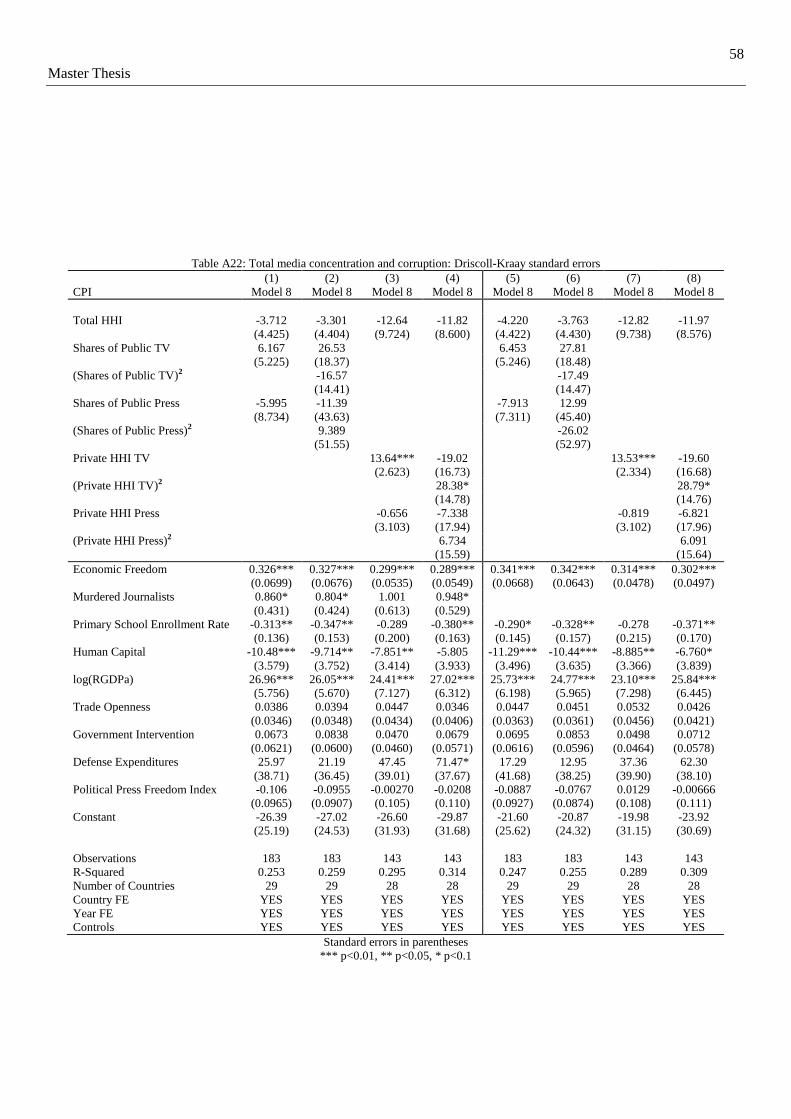
58

Master Thesis

Table A22: Total media concentration and corruption: Driscoll-Kraay standard errors

(1) (2) (3) (4) (5) (6) (7) (8)

CPI Model 8 Model 8 Model 8 Model 8 Model 8 Model 8 Model 8 Model 8

Total HHI -3.712 -3.301 -12.64 -11.82 -4.220 -3.763 -12.82 -11.97

(4.425) (4.404) (9.724) (8.600) (4.422) (4.430) (9.738) (8.576)

Shares of Public TV 6.167 26.53 6.453 27.81

(5.225) (18.37) (5.246) (18.48)

(Shares of Public TV)2 -16.57 -17.49

(14.41) (14.47)

Shares of Public Press -5.995 -11.39 -7.913 12.99

(8.734) (43.63) (7.311) (45.40)

(Shares of Public Press)2 9.389 -26.02

(51.55) (52.97)

Private HHI TV 13.64*** -19.02 13.53*** -19.60

(2.623) (16.73) (2.334) (16.68)

(Private HHI TV)2 28.38* 28.79*

(14.78) (14.76)

Private HHI Press -0.656 -7.338 -0.819 -6.821

(3.103) (17.94) (3.102) (17.96)

(Private HHI Press)2 6.734 6.091

(15.59) (15.64)

Economic Freedom 0.326*** 0.327*** 0.299*** 0.289*** 0.341*** 0.342*** 0.314*** 0.302***

(0.0699) (0.0676) (0.0535) (0.0549) (0.0668) (0.0643) (0.0478) (0.0497)

Murdered Journalists 0.860* 0.804* 1.001 0.948*

(0.431) (0.424) (0.613) (0.529)

Primary School Enrollment Rate -0.313** -0.347** -0.289 -0.380** -0.290* -0.328** -0.278 -0.371**

(0.136) (0.153) (0.200) (0.163) (0.145) (0.157) (0.215) (0.170)

Human Capital -10.48*** -9.714** -7.851** -5.805 -11.29*** -10.44*** -8.885** -6.760*

(3.579) (3.752) (3.414) (3.933) (3.496) (3.635) (3.366) (3.839)

log(RGDPa) 26.96*** 26.05*** 24.41*** 27.02*** 25.73*** 24.77*** 23.10*** 25.84***

(5.756) (5.670) (7.127) (6.312) (6.198) (5.965) (7.298) (6.445)

Trade Openness 0.0386 0.0394 0.0447 0.0346 0.0447 0.0451 0.0532 0.0426

(0.0346) (0.0348) (0.0434) (0.0406) (0.0363) (0.0361) (0.0456) (0.0421)

Government Intervention 0.0673 0.0838 0.0470 0.0679 0.0695 0.0853 0.0498 0.0712

(0.0621) (0.0600) (0.0460) (0.0571) (0.0616) (0.0596) (0.0464) (0.0578)

Defense Expenditures 25.97 21.19 47.45 71.47* 17.29 12.95 37.36 62.30

(38.71) (36.45) (39.01) (37.67) (41.68) (38.25) (39.90) (38.10)

Political Press Freedom Index -0.106 -0.0955 -0.00270 -0.0208 -0.0887 -0.0767 0.0129 -0.00666

(0.0965) (0.0907) (0.105) (0.110) (0.0927) (0.0874) (0.108) (0.111)

Constant -26.39 -27.02 -26.60 -29.87 -21.60 -20.87 -19.98 -23.92

(25.19) (24.53) (31.93) (31.68) (25.62) (24.32) (31.15) (30.69)

Observations 183 183 143 143 183 183 143 143

R-Squared 0.253 0.259 0.295 0.314 0.247 0.255 0.289 0.309

Number of Countries 29 29 28 28 29 29 28 28

Country FE YES YES YES YES YES YES YES YES

Year FE YES YES YES YES YES YES YES YES

Controls YES YES YES YES YES YES YES YES

Standard errors in parentheses

*** p<0.01, ** p<0.05, * p<0.1

59

Master Thesis

Table A23: Total media concentration and heterogeneous effects (1) (2) (3) (4) (5) (6) (7) (8) (9) (10) (11) (12) (13) (14) (15) (16)

CPI Model 5 Model 5 Model 5 Model 5 Model 5 Model 5 Model 5 Model 5 Model 5 Model 5 Model 5 Model 5 Model 5 Model 5 Model 5 Model 5

Total HHI * EF 0.115 0.0118

(0.132) (0.152)

Total HHI * PS -0.363 -0.252

(0.291) (0.277)

Total HHI * HC -0.642 -0.453

(1.730) (1.928)

Total HHI * LR 5.923 1.888

(3.745) (4.507)

Total HHI * TO 0.0787* 0.0784

(0.0457) (0.0613)

Total HHI * GI -0.0259 -0.0656

(0.0654) (0.0887)

Total HHI * DE -56.91 -89.00*

(35.11) (44.11)

Total HHI * PF -0.207 0.0232

(0.193) (0.247)

Total HHI -8.788 33.78 0.856 -26.06 -6.102* 0.493 2.768 1.175 -1.796 23.04 0.252 -9.107 -6.084 2.718 4.477 -1.260

(8.870) (27.68) (4.730) (15.85) (3.471) (5.289) (3.897) (3.493) (9.865) (25.73) (5.471) (18.20) (4.275) (6.558) (4.292) (4.053)

Economic

Freedom

0.186 0.169 0.211 0.150 0.202* 0.223** 0.167 0.164 0.181 0.171 0.166 0.150 0.153 0.194 0.169

(0.123) (0.126) (0.127) (0.121) (0.110) (0.106) (0.126) (0.147) (0.125) (0.128) (0.128) (0.126) (0.137) (0.115) (0.125)

Primary School

Enrollment

-0.278 -0.279 -0.204 -0.238 -0.272 -0.241 -0.243 -0.281 -0.118 -0.281 -0.282 -0.238 -0.289 -0.258 -0.282

(0.219) (0.223) (0.220) (0.201) (0.214) (0.202) (0.227) (0.223) (0.162) (0.223) (0.221) (0.197) (0.217) (0.199) (0.221)

Human Capital -1.079 -1.828 1.147 -1.417 -1.226 -1.922 -2.737 -1.314 -1.703 -1.075 -1.058 -1.431 -1.052 -0.384 -1.226

(3.861) (3.761) (3.875) (4.062) (3.964) (3.911) (3.847) (4.004) (3.881) (4.213) (4.053) (3.871) (3.940) (3.857) (3.978)

Log(RGDPa) 21.47** 19.53** 20.03** 19.27** 19.76** 12.57 17.57** 20.13** 20.17** 20.37** 18.36* 19.26** 20.12** 17.10** 20.17**

(8.842) (8.616) (8.258) (8.716) (8.210) (7.714) (8.054) (8.584) (8.612) (8.568) (10.69) (8.397) (8.062) (8.016) (8.383)

Trade Openness 0.0335 0.0338 0.0309 0.0482 0.0327 0.0355 0.0384 0.0345 0.0362 0.0340 0.0351 0.000534 0.0337 0.0298 0.0344

(0.0387) (0.0364) (0.0383) (0.0426) (0.0379) (0.0386) (0.0399) (0.0383) (0.0376) (0.0380) (0.0382) (0.0557) (0.0386) (0.0386) (0.0382)

Government

Intervention

0.0438 0.00756 0.0161 0.0232 0.0324 0.0202 0.0267 0.0178 0.0116 0.0164 0.0211 0.0324 0.0518 0.0273 0.0169

(0.0540) (0.0571) (0.0594) (0.0627) (0.0585) (0.0576) (0.0590) (0.0589) (0.0587) (0.0599) (0.0607) (0.0592) (0.0791) (0.0582) (0.0573)

Defense

Expenditures

10.94 -1.457 7.767 -43.63 1.155 5.700 -7.562 4.096 1.599 5.102 4.717 1.124 12.33 74.85 4.890

(43.24) (42.54) (43.31) (30.55) (40.65) (39.06) (40.82) (43.21) (41.90) (41.06) (39.95) (39.92) (40.95) (50.34) (40.73)

Political Press

Freedom

-0.245* -0.241* -0.252* -0.153 -0.257* -0.259* -0.161 -0.246* -0.248* -0.245* -0.244* -0.257* -0.248* -0.170 -0.257

(0.127) (0.121) (0.123) (0.126) (0.131) (0.133) (0.133) (0.129) (0.126) (0.128) (0.130) (0.126) (0.129) (0.131) (0.168)

Murdered

Journalists

1.065* 1.037* 1.013** 0.797 1.011* 0.975* 0.980* 0.862 1.021* 1.029* 1.027* 0.989* 1.011* 0.946* 0.970** 1.023*

(0.527) (0.556) (0.493) (0.583) (0.586) (0.538) (0.504) (0.610) (0.526) (0.545) (0.515) (0.529) (0.586) (0.551) (0.454) (0.514)

Constant -4.974 -31.10 -11.21 63.00** -4.805 -8.349 18.53 1.316 -7.369 -22.94 -9.595 -0.778 -4.694 -8.814 -6.531 -7.959

(42.94) (38.35) (41.74) (24.53) (40.57) (37.42) (36.67) (36.46) (44.48) (38.28) (41.63) (49.67) (35.36) (37.79) (36.33) (39.18)

Observations 377 377 377 377 377 377 377 377 377 377 377 377 377 377 377 377

R-squared 0.135 0.144 0.142 0.121 0.157 0.142 0.159 0.132 0.142 0.146 0.142 0.143 0.157 0.147 0.169 0.142

Number of

Countries

29 29 29 29 29 29 29 29 29 29 29 29 29 29 29 29

Country FE YES YES YES YES YES YES YES YES YES YES YES YES YES YES YES YES

Year FE YES YES YES YES YES YES YES YES YES YES YES YES YES YES YES YES

Controls YES YES YES YES YES YES YES YES YES YES YES YES YES YES YES YES

Robust standard errors in parentheses. Standard errors are clustered by countries.

*** p<0.01, ** p<0.05, * p<0.1

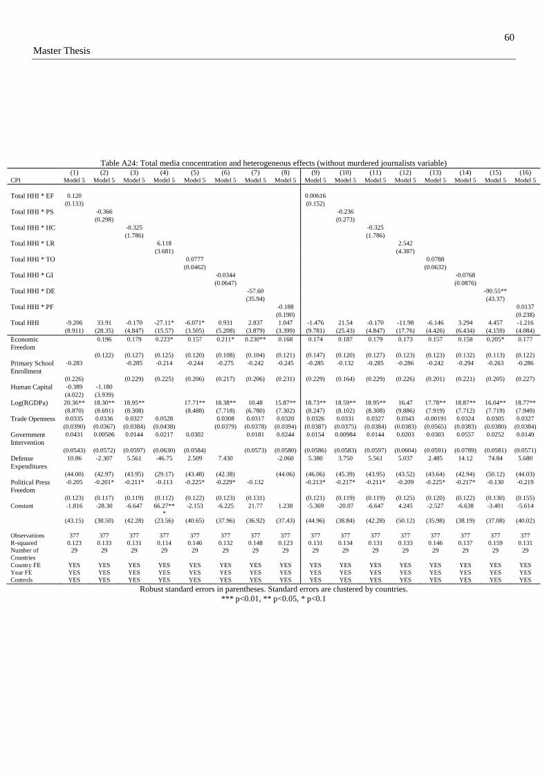
60

Master Thesis

Table A24: Total media concentration and heterogeneous effects (without murdered journalists variable) (1) (2) (3) (4) (5) (6) (7) (8) (9) (10) (11) (12) (13) (14) (15) (16) CPI Model 5 Model 5 Model 5 Model 5 Model 5 Model 5 Model 5 Model 5 Model 5 Model 5 Model 5 Model 5 Model 5 Model 5 Model 5 Model 5

Total HHI * EF 0.120 0.00616

(0.133) (0.152)

Total HHI * PS -0.366 -0.236

(0.298) (0.273)

Total HHI * HC -0.325 -0.325

(1.786) (1.786)

Total HHI * LR 6.118 2.542

(3.681) (4.387)

Total HHI * TO 0.0777 0.0788

(0.0462) (0.0632)

Total HHI * GI -0.0344 -0.0768

(0.0647) (0.0876)

Total HHI * DE -57.60 -90.55**

(35.94) (43.37)

Total HHI * PF -0.188 0.0137

(0.190) (0.238)

Total HHI -9.206 33.91 -0.170 -27.11* -6.071* 0.931 2.837 1.047 -1.476 21.54 -0.170 -11.98 -6.146 3.294 4.457 -1.216

(8.911) (28.35) (4.847) (15.57) (3.505) (5.208) (3.879) (3.399) (9.781) (25.43) (4.847) (17.76) (4.426) (6.434) (4.159) (4.084)

Economic

Freedom

0.196 0.179 0.223* 0.157 0.211* 0.230** 0.168 0.174 0.187 0.179 0.173 0.157 0.158 0.205* 0.177

(0.122) (0.127) (0.125) (0.120) (0.108) (0.104) (0.121) (0.147) (0.120) (0.127) (0.123) (0.123) (0.132) (0.113) (0.122)

Primary School

Enrollment

-0.283 -0.285 -0.214 -0.244 -0.275 -0.242 -0.245 -0.285 -0.132 -0.285 -0.286 -0.242 -0.294 -0.263 -0.286

(0.226) (0.229) (0.225) (0.206) (0.217) (0.206) (0.231) (0.229) (0.164) (0.229) (0.226) (0.201) (0.221) (0.205) (0.227)

Human Capital -0.389 -1.180

(4.022) (3.939)

Log(RGDPa) 20.36** 18.30** 18.95** 17.71** 18.38** 10.48 15.87** 18.73** 18.59** 18.95** 16.47 17.78** 18.87** 16.04** 18.77**

(8.870) (8.691) (8.308) (8.488) (7.718) (6.780) (7.302) (8.247) (8.102) (8.308) (9.886) (7.919) (7.712) (7.719) (7.949)

Trade Openness 0.0335 0.0336 0.0327 0.0528 0.0308 0.0317 0.0320 0.0326 0.0331 0.0327 0.0343 -0.00191 0.0324 0.0305 0.0327

(0.0390) (0.0367) (0.0384) (0.0438) (0.0379) (0.0378) (0.0394) (0.0387) (0.0375) (0.0384) (0.0383) (0.0565) (0.0383) (0.0380) (0.0384)

Government Intervention

0.0431 0.00506 0.0144 0.0217 0.0302 0.0181 0.0244 0.0154 0.00984 0.0144 0.0203 0.0303 0.0557 0.0252 0.0149

(0.0543) (0.0572) (0.0597) (0.0630) (0.0584) (0.0573) (0.0580) (0.0586) (0.0583) (0.0597) (0.0604) (0.0591) (0.0789) (0.0581) (0.0571)

Defense

Expenditures

10.86 -2.307 5.561 -46.75 2.509 7.430 -2.060 5.380 3.750 5.561 5.037 2.485 14.12 74.84 5.680

(44.00) (42.97) (43.95) (29.17) (43.48) (42.38) (44.06) (46.06) (45.39) (43.95) (43.52) (43.64) (42.94) (50.12) (44.03)

Political Press

Freedom

-0.205 -0.201* -0.211* -0.113 -0.225* -0.229* -0.132 -0.213* -0.217* -0.211* -0.209 -0.225* -0.217* -0.130 -0.219

(0.123) (0.117) (0.119) (0.112) (0.122) (0.123) (0.131) (0.121) (0.119) (0.119) (0.125) (0.120) (0.122) (0.130) (0.155)

Constant -1.816 -28.30 -6.647 66.27**

*

-2.153 -6.225 21.77 1.238 -5.369 -20.07 -6.647 4.245 -2.527 -6.638 -3.401 -5.614

(43.15) (38.50) (42.28) (23.56) (40.65) (37.96) (36.92) (37.43) (44.96) (38.84) (42.28) (50.12) (35.98) (38.19) (37.08) (40.02)

Observations 377 377 377 377 377 377 377 377 377 377 377 377 377 377 377 377

R-squared 0.123 0.133 0.131 0.114 0.146 0.132 0.148 0.123 0.131 0.134 0.131 0.133 0.146 0.137 0.159 0.131

Number of

Countries

29 29 29 29 29 29 29 29 29 29 29 29 29 29 29 29

Country FE YES YES YES YES YES YES YES YES YES YES YES YES YES YES YES YES

Year FE YES YES YES YES YES YES YES YES YES YES YES YES YES YES YES YES

Controls YES YES YES YES YES YES YES YES YES YES YES YES YES YES YES YES

Robust standard errors in parentheses. Standard errors are clustered by countries.

*** p<0.01, ** p<0.05, * p<0.1

61

Master Thesis

Table A25: Total media concentration and additional heterogeneous effects (without murdered journalists variable)

(1) (2) (3) (4) (5) (6) (7) (8)

CPI Model 5 Model 5 Model 5 Model 5 Model 5 Model 5 Model 5 Model 5

Total HHI * Public TV 17.64** 15.86

(7.591) (11.47)

Total HHI * Public Press -0.759 -1.910

(7.792) (9.950)

Total HHI * Private HHI TV -9.909 -10.32

(6.324) (8.341)

Total HHI * Private HHI Press 5.233 19.68

(7.075) (19.19)

Public TV 2.098

(8.440)

Public Press 2.155

(8.539)

Private HHI TV 0.430

(7.592)

Private HHI Press -6.730

(8.128)

Total HHI -8.976 -3.112 2.537 -10.66 -8.301 -3.082 2.835 -13.45

(5.518) (2.876) (7.116) (8.791) (6.049) (2.897) (8.633) (9.929)

Economic Freedom 0.247* 0.331** 0.249* 0.387** 0.252* 0.332** 0.249* 0.388**

(0.126) (0.154) (0.137) (0.146) (0.129) (0.153) (0.137) (0.146)

Primary School Enrollment Rate -0.287 -0.219 -0.310 -0.433 -0.294 -0.221 -0.312 -0.446

(0.241) (0.237) (0.234) (0.270) (0.246) (0.239) (0.227) (0.275)

Human Capital -5.095 -9.913** -4.803 -11.11* -4.978 -9.906** -4.823 -10.81*

(4.680) (4.779) (5.085) (5.541) (4.706) (4.779) (5.138) (5.522)

log(RGDPa) 28.07*** 21.25** 34.21*** 17.92** 27.91*** 21.22** 34.20*** 17.51*

(8.123) (8.813) (9.939) (8.580) (8.243) (8.783) (9.962) (8.598)

Trade Openness 0.0495 0.0553 0.0321 0.0723 0.0497 0.0550 0.0324 0.0697

(0.0410) (0.0457) (0.0373) (0.0485) (0.0408) (0.0461) (0.0368) (0.0482)

Government Intervention 0.0476 0.0430 0.0176 0.0454 0.0479 0.0427 0.0180 0.0438

(0.0753) (0.0768) (0.0852) (0.0706) (0.0744) (0.0767) (0.0825) (0.0715)

Defense Expenditures 52.31 -20.63 98.00* -30.34 52.83 -19.53 97.97* -31.25

(52.55) (53.10) (55.16) (59.13) (52.91) (53.98) (55.35) (60.24)

Political Press Freedom -0.178 -0.160 -0.225 -0.0918 -0.175 -0.162 -0.223 -0.105

(0.178) (0.176) (0.196) (0.194) (0.179) (0.178) (0.196) (0.193)

Constant -45.10 -3.829 -69.20 29.04 -45.28 -3.893 -69.25 33.30

(39.65) (49.49) (43.91) (43.62) (39.71) (49.63) (44.17) (43.45)

Observations 203 305 198 188 203 305 198 188

R-squared 0.224 0.200 0.228 0.278 0.225 0.200 0.228 0.280

Number of Countries 29 29 29 29 29 29 29 29

Country FE YES YES YES YES YES YES YES YES

Year FE YES YES YES YES YES YES YES YES

Controls YES YES YES YES YES YES YES YES

Robust standard errors in parentheses. Standard errors are clustered by countries.

*** p<0.01, ** p<0.05, * p<0.1

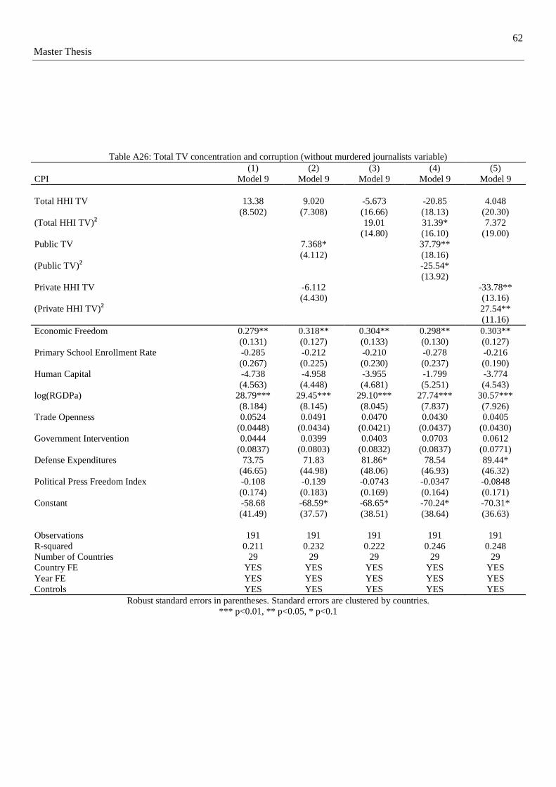
62

Master Thesis

Table A26: Total TV concentration and corruption (without murdered journalists variable)

(1) (2) (3) (4) (5)

CPI Model 9 Model 9 Model 9 Model 9 Model 9

Total HHI TV 13.38 9.020 -5.673 -20.85 4.048

(8.502) (7.308) (16.66) (18.13) (20.30)

(Total HHI TV)2

19.01 31.39* 7.372

(14.80) (16.10) (19.00)

Public TV 7.368* 37.79**

(4.112) (18.16)

(Public TV)2

-25.54*

(13.92)

Private HHI TV -6.112 -33.78**

(4.430) (13.16)

(Private HHI TV)2

27.54**

(11.16)

Economic Freedom 0.279** 0.318** 0.304** 0.298** 0.303**

(0.131) (0.127) (0.133) (0.130) (0.127)

Primary School Enrollment Rate -0.285 -0.212 -0.210 -0.278 -0.216

(0.267) (0.225) (0.230) (0.237) (0.190)

Human Capital -4.738 -4.958 -3.955 -1.799 -3.774

(4.563) (4.448) (4.681) (5.251) (4.543)

log(RGDPa) 28.79*** 29.45*** 29.10*** 27.74*** 30.57***

(8.184) (8.145) (8.045) (7.837) (7.926)

Trade Openness 0.0524 0.0491 0.0470 0.0430 0.0405

(0.0448) (0.0434) (0.0421) (0.0437) (0.0430)

Government Intervention 0.0444 0.0399 0.0403 0.0703 0.0612

(0.0837) (0.0803) (0.0832) (0.0837) (0.0771)

Defense Expenditures 73.75 71.83 81.86* 78.54 89.44*

(46.65) (44.98) (48.06) (46.93) (46.32)

Political Press Freedom Index -0.108 -0.139 -0.0743 -0.0347 -0.0848

(0.174) (0.183) (0.169) (0.164) (0.171)

Constant -58.68 -68.59* -68.65* -70.24* -70.31*

(41.49) (37.57) (38.51) (38.64) (36.63)

Observations 191 191 191 191 191

R-squared 0.211 0.232 0.222 0.246 0.248

Number of Countries 29 29 29 29 29

Country FE YES YES YES YES YES

Year FE YES YES YES YES YES

Controls YES YES YES YES YES

Robust standard errors in parentheses. Standard errors are clustered by countries.

*** p<0.01, ** p<0.05, * p<0.1

63

Master Thesis

Table A27: Total TV concentration and heterogeneous effects (1) (2) (3) (4) (5) (6) (7) (8) (9) (10) (11) (12) (13) (14)

CPI Model 5 Model 5 Model 5 Model 5 Model 5 Model 5 Model 5 Model 5 Model 5 Model 5 Model 5 Model 5 Model 5 Model 5

Total HHI TV * EF 0.267 -0.257

(0.372) (0.501)

Total HHI TV * HC 3.319 8.386

(8.133) (10.33)

Total HHI TV * LR 25.88*** 11.36

(6.638) (15.21)

Total HHI TV * TO 0.0432 -0.00593 (0.0783) (0.133)

Total HHI TV * GI -0.0937 -0.371*

(0.176) (0.197)

Total HHI TV * DE 21.88 -103.8

(85.25) (100.0)

Total HHI TV * PF -0.00268 0.415

(0.261) (0.362) Total HHI TV -3.827 4.072 -93.53*** 9.416 16.42 12.60 13.78* 27.97 -7.602 -33.94 13.22 33.13** 18.32* 8.351

(22.21) (20.67) (26.04) (7.808) (11.49) (10.47) (7.830) (30.74) (24.38) (60.55) (10.98) (14.62) (10.67) (10.31)

Economic Freedom 0.204 0.269** 0.229 0.329** 0.257* 0.233 0.302 0.232* 0.240* 0.228 0.227* 0.237* 0.234*

(0.140) (0.125) (0.139) (0.146) (0.136) (0.139) (0.180) (0.137) (0.132) (0.139) (0.130) (0.135) (0.129)

Human Capital -3.190 -0.528 -2.883 -3.864 -6.700 -5.791 -4.404 -6.770 -2.747 -4.364 -3.591 -4.117 -3.571

(4.562) (4.712) (4.837) (4.159) (4.434) (4.329) (4.365) (6.345) (4.223) (4.637) (4.242) (4.529) (4.502)

Log(RGDPa) 34.11*** 31.32*** 32.89*** 32.48*** 23.60* 28.77*** 31.72*** 31.16*** 21.64 32.42*** 31.40*** 25.30* 30.57***

(9.146) (8.796) (8.926) (9.590) (12.93) (8.999) (9.135) (9.202) (18.42) (8.766) (8.925) (13.29) (9.123)

Trade Openness 0.0396 0.0297 0.0749 0.0335 0.0541 0.0496 0.0374 0.0535 0.0506 0.0435 0.0441 0.0554 0.0392

(0.0452) (0.0449) (0.0489) (0.0408) (0.0439) (0.0453) (0.0434) (0.0459) (0.0443) (0.0763) (0.0418) (0.0440) (0.0433) Government

Intervention

0.0833 0.0537 0.0844 0.0491 0.0530 0.0593 0.0482 0.0605 0.0658 0.0523 0.180* 0.0722 0.0499

(0.0815) (0.0844) (0.0887) (0.0832) (0.0909) (0.0848) (0.0841) (0.0853) (0.0875) (0.0831) (0.102) (0.0922) (0.0822)

Defense

Expenditures

102.5** 113.3** 71.16* 98.01** 101.5** 75.54 87.47* 104.0** 97.71** 90.87* 113.3** 140.2*** 93.41**

(46.66) (46.89) (39.92) (47.23) (48.01) (44.94) (47.97) (46.32) (44.97) (48.05) (52.57) (50.18) (44.52)

Political Press Freedom

-0.159 -0.209 -0.0416 -0.172 -0.194 -0.0909 -0.152 -0.163 -0.130 -0.152 -0.182 -0.0912 -0.354

(0.184) (0.173) (0.149) (0.187) (0.193) (0.205) (0.180) (0.180) (0.196) (0.186) (0.189) (0.216) (0.254)

Murdered

Journalists

2.105*** 1.960** 1.340** 1.977*** 1.753** 1.752*** 1.838** 2.040*** 1.808** 1.778** 1.985*** 1.548** 1.804** 1.944***

(0.720) (0.719) (0.496) (0.652) (0.685) (0.619) (0.697) (0.717) (0.690) (0.702) (0.667) (0.597) (0.680) (0.690)

Primary School

Enrollment

-0.333 -0.339 -0.250 -0.249 -0.244 -0.211 -0.224 -0.233 -0.328 -0.284 -0.282 -0.282 -0.287 -0.239

(0.229) (0.224) (0.205) (0.226) (0.218) (0.237) (0.237) (0.236) (0.228) (0.224) (0.251) (0.192) (0.230) (0.245) Constant -65.85 -73.53* 45.73* -79.22* -80.34* -32.95 -61.14 -78.19* -58.89 -33.75 -72.95* -77.70* -48.07 -69.91

(41.20) (42.77) (22.98) (41.31) (44.51) (55.45) (43.86) (44.72) (46.62) (68.76) (42.48) (44.02) (53.39) (41.52)

Observations 191 191 191 191 191 191 191 191 191 191 191 191 191 191

R-squared 0.224 0.234 0.229 0.235 0.236 0.217 0.232 0.240 0.244 0.244 0.238 0.273 0.247 0.247

Number of

Countries

29 29 29 29 29 29 29 29 29 29 29 29 29 29

Country FE YES YES YES YES YES YES YES YES YES YES YES YES YES YES Year FE YES YES YES YES YES YES YES YES YES YES YES YES YES YES

Controls YES YES YES YES YES YES YES YES YES YES YES YES YES YES

Robust standard errors in parentheses. Standard errors are clustered by countries.

*** p<0.01, ** p<0.05, * p<0.1

64

Master Thesis

Table A28: Total TV concentration heterogeneous effects (without murdered journalists variable) (1) (2) (3) (4) (5) (6) (7) (8) (9) (10) (11) (12) (13) (14)

CPI Model 5 Model 5 Model 5 Model 5 Model 5 Model 5 Model 5 Model 5 Model 5 Model 5 Model 5 Model 5 Model 5 Model 5

Total HHI TV * EF 0.421 -0.138

(0.365) (0.491)

Total HHI TV * HC 5.394 11.20

(8.355) (10.26)

Total HHI TV * LR 25.56*** 15.86

(6.722) (15.02) Total HHI TV * TO 0.0684 0.0210

(0.0888) (0.146)

Total HHI TV * GI -0.130 -0.419**

(0.173) (0.193)

Total HHI TV * DE -6.157 -129.9

(81.98) (100.3)

Total HHI TV * PF 0.0554 0.436

(0.240) (0.348) Total HHI TV -12.36 -0.594 -91.88*** 8.360 18.76 14.53 13.57 21.52 -13.99 -52.01 12.03 36.17** 20.18* 8.655

(22.12) (20.67) (25.96) (8.025) (11.42) (10.67) (8.327) (29.85) (23.70) (59.08) (11.22) (14.52) (11.09) (10.68)

Economic Freedom 0.248* 0.299** 0.281** 0.379** 0.302** 0.279** 0.319* 0.278** 0.287** 0.281** 0.265** 0.283** 0.283**

(0.134) (0.122) (0.133) (0.142) (0.132) (0.134) (0.182) (0.134) (0.125) (0.132) (0.127) (0.129) (0.124)

Human Capital -3.544 -0.971 -2.988 -4.179 -7.005 -5.987 -4.815 -8.017 -2.538 -4.422 -3.852 -4.489 -3.989

(4.677) (4.704) (4.982) (4.326) (4.517) (4.426) (4.541) (6.406) (4.353) (4.818) (4.269) (4.653) (4.680)

Log(RGDPa) 30.81*** 27.46*** 29.03*** 29.35*** 18.84 25.54*** 28.40*** 27.62*** 14.35 28.56*** 28.60*** 20.36 26.99***

(8.409) (8.118) (8.436) (8.894) (11.99) (8.052) (8.311) (8.377) (17.68) (8.217) (8.325) (12.22) (8.259)

Trade Openness 0.0536 0.0410 0.0796 0.0433 0.0678 0.0595 0.0508 0.0682 0.0646 0.0421 0.0534 0.0695 0.0506

(0.0474) (0.0459) (0.0499) (0.0413) (0.0454) (0.0464) (0.0457) (0.0479) (0.0468) (0.0786) (0.0422) (0.0457) (0.0449) Government

Intervention

0.0790 0.0477 0.0780 0.0412 0.0514 0.0510 0.0421 0.0562 0.0643 0.0443 0.191* 0.0701 0.0420

(0.0826) (0.0856) (0.0883) (0.0840) (0.0916) (0.0854) (0.0858) (0.0868) (0.0890) (0.0839) (0.104) (0.0936) (0.0832)

Defense

Expenditures

86.87* 103.0** 68.44* 81.64* 89.06* 61.11 71.52 92.94* 85.46* 74.68 103.1* 137.1** 76.50*

(46.00) (46.18) (39.76) (47.96) (47.92) (42.93) (46.79) (45.51) (43.44) (47.59) (52.69) (52.82) (44.43)

Political Press Freedom

-0.113 -0.179 -0.0271 -0.131 -0.160 -0.0370 -0.107 -0.127 -0.0826 -0.111 -0.152 -0.0357 -0.320

(0.177) (0.163) (0.143) (0.183) (0.185) (0.193) (0.173) (0.172) (0.186) (0.179) (0.180) (0.204) (0.248)

Primary School

Enrollment

-0.367 -0.365 -0.265 -0.245 -0.247 -0.220 -0.229 -0.260 -0.350 -0.291 -0.276 -0.286 -0.294 -0.242

(0.259) (0.257) (0.219) (0.252) (0.236) (0.258) (0.265) (0.268) (0.257) (0.242) (0.276) (0.207) (0.252) (0.275)

Constant -47.60 -57.36 46.58* -65.03 -68.91 -14.83 -48.45 -61.25 -41.50 -5.940 -58.92 -67.53 -29.09 -55.72

(38.16) (41.94) (23.52) (41.42) (43.29) (53.63) (41.99) (42.82) (45.27) (66.97) (41.63) (42.77) (50.70) (40.75)

Observations 191 191 191 191 191 191 191 191 191 191 191 191 191 191

R-squared 0.193 0.208 0.216 0.208 0.215 0.196 0.208 0.211 0.222 0.223 0.211 0.257 0.224 0.220

Number of

Countries

29 29 29 29 29 29 29 29 29 29 29 29 29 29

Country FE YES YES YES YES YES YES YES YES YES YES YES YES YES YES

Year FE YES YES YES YES YES YES YES YES YES YES YES YES YES YES

Controls YES YES YES YES YES YES YES YES YES YES YES YES YES YES

Robust standard errors in parentheses. Standard errors are clustered by countries.

*** p<0.01, ** p<0.05, * p<0.1

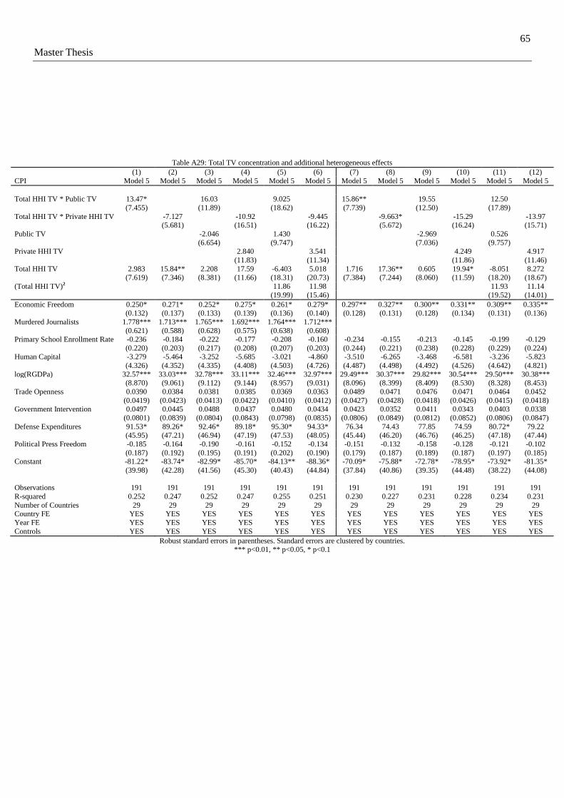
65

Master Thesis

Table A29: Total TV concentration and additional heterogeneous effects

(1) (2) (3) (4) (5) (6) (7) (8) (9) (10) (11) (12)

CPI Model 5 Model 5 Model 5 Model 5 Model 5 Model 5 Model 5 Model 5 Model 5 Model 5 Model 5 Model 5

Total HHI TV * Public TV 13.47* 16.03 9.025 15.86** 19.55 12.50

(7.455) (11.89) (18.62) (7.739) (12.50) (17.89)

Total HHI TV * Private HHI TV -7.127 -10.92 -9.445 -9.663* -15.29 -13.97 (5.681) (16.51) (16.22) (5.672) (16.24) (15.71)

Public TV -2.046 1.430 -2.969 0.526

(6.654) (9.747) (7.036) (9.757) Private HHI TV 2.840 3.541 4.249 4.917

(11.83) (11.34) (11.86) (11.46)

Total HHI TV 2.983 15.84** 2.208 17.59 -6.403 5.018 1.716 17.36** 0.605 19.94* -8.051 8.272 (7.619) (7.346) (8.381) (11.66) (18.31) (20.73) (7.384) (7.244) (8.060) (11.59) (18.20) (18.67)

(Total HHI TV)2 11.86 11.98 11.93 11.14

(19.99) (15.46) (19.52) (14.01)

Economic Freedom 0.250* 0.271* 0.252* 0.275* 0.261* 0.279* 0.297** 0.327** 0.300** 0.331** 0.309** 0.335** (0.132) (0.137) (0.133) (0.139) (0.136) (0.140) (0.128) (0.131) (0.128) (0.134) (0.131) (0.136)

Murdered Journalists 1.778*** 1.713*** 1.765*** 1.692*** 1.764*** 1.712***

(0.621) (0.588) (0.628) (0.575) (0.638) (0.608) Primary School Enrollment Rate -0.236 -0.184 -0.222 -0.177 -0.208 -0.160 -0.234 -0.155 -0.213 -0.145 -0.199 -0.129

(0.220) (0.203) (0.217) (0.208) (0.207) (0.203) (0.244) (0.221) (0.238) (0.228) (0.229) (0.224) Human Capital -3.279 -5.464 -3.252 -5.685 -3.021 -4.860 -3.510 -6.265 -3.468 -6.581 -3.236 -5.823

(4.326) (4.352) (4.335) (4.408) (4.503) (4.726) (4.487) (4.498) (4.492) (4.526) (4.642) (4.821)

log(RGDPa) 32.57*** 33.03*** 32.78*** 33.11*** 32.46*** 32.97*** 29.49*** 30.37*** 29.82*** 30.54*** 29.50*** 30.38*** (8.870) (9.061) (9.112) (9.144) (8.957) (9.031) (8.096) (8.399) (8.409) (8.530) (8.328) (8.453)

Trade Openness 0.0390 0.0384 0.0381 0.0385 0.0369 0.0363 0.0489 0.0471 0.0476 0.0471 0.0464 0.0452

(0.0419) (0.0423) (0.0413) (0.0422) (0.0410) (0.0412) (0.0427) (0.0428) (0.0418) (0.0426) (0.0415) (0.0418) Government Intervention 0.0497 0.0445 0.0488 0.0437 0.0480 0.0434 0.0423 0.0352 0.0411 0.0343 0.0403 0.0338

(0.0801) (0.0839) (0.0804) (0.0843) (0.0798) (0.0835) (0.0806) (0.0849) (0.0812) (0.0852) (0.0806) (0.0847)

Defense Expenditures 91.53* 89.26* 92.46* 89.18* 95.30* 94.33* 76.34 74.43 77.85 74.59 80.72* 79.22 (45.95) (47.21) (46.94) (47.19) (47.53) (48.05) (45.44) (46.20) (46.76) (46.25) (47.18) (47.44)

Political Press Freedom -0.185 -0.164 -0.190 -0.161 -0.152 -0.134 -0.151 -0.132 -0.158 -0.128 -0.121 -0.102

(0.187) (0.192) (0.195) (0.191) (0.202) (0.190) (0.179) (0.187) (0.189) (0.187) (0.197) (0.185) Constant -81.22* -83.74* -82.99* -85.70* -84.13** -88.36* -70.09* -75.88* -72.78* -78.95* -73.92* -81.35*

(39.98) (42.28) (41.56) (45.30) (40.43) (44.84) (37.84) (40.86) (39.35) (44.48) (38.22) (44.08)

Observations 191 191 191 191 191 191 191 191 191 191 191 191

R-squared 0.252 0.247 0.252 0.247 0.255 0.251 0.230 0.227 0.231 0.228 0.234 0.231

Number of Countries 29 29 29 29 29 29 29 29 29 29 29 29 Country FE YES YES YES YES YES YES YES YES YES YES YES YES

Year FE YES YES YES YES YES YES YES YES YES YES YES YES

Controls YES YES YES YES YES YES YES YES YES YES YES YES

Robust standard errors in parentheses. Standard errors are clustered by countries. *** p<0.01, ** p<0.05, * p<0.1

66

Master Thesis

Table A30: Total press concentration and corruption

(1) (2) (3) (4) (5) (6) (7) (8) (9) (10)

CPI Model 9 Model 9 Model 9 Model 9 Model 9 Model 9 Model 9 Model 9 Model 9 Model 9

Total HHI Press -39.45*** -5.519 16.40 -13.45 -28.79 4.096 -24.75 5.840 84.91 -1.448

(4.959) (6.981) (16.00) (12.12) (39.74) (34.99) (50.65) (33.55) (68.40) (35.46)

(Total HHI Press)2 -9.393 -17.10 20.29 -25.87 -125.7* -20.27

(34.15) (61.53) (99.98) (59.14) (73.02) (59.17)

Public Press -57.81*** -0.606 -123.2** 24.63

(13.58) (5.405) (56.51) (15.39)

(Public Press)2 88.63 -41.63

(109.7) (26.64)

Private HHI Press -38.09*** 5.507 -74.40 0.479

(12.80) (6.106) (95.57) (19.71)

(Private HHI Press)2 9.061 4.509

(88.80) (15.94)

Economic Freedom 0.372** 0.398** 0.371** 0.382** 0.397**

(0.141) (0.154) (0.141) (0.143) (0.155)

Primary School Enrollment Rate -0.392 -0.404 -0.395 -0.389 -0.411

(0.256) (0.267) (0.253) (0.255) (0.264)

Human Capital -10.02* -10.53* -9.968* -10.38* -10.51*

(5.609) (5.559) (5.586) (5.594) (5.571)

log(RGDPa) 16.75** 17.19** 16.59** 16.86** 16.81**

(7.271) (7.144) (7.452) (7.377) (7.383)

Trade Openness 0.0693 0.0700 0.0692 0.0698 0.0702

(0.0496) (0.0513) (0.0500) (0.0514) (0.0509)

Government Intervention 0.0410 0.0439 0.0402 0.0417 0.0415

(0.0759) (0.0769) (0.0760) (0.0773) (0.0772)

Defense Expenditures -45.62 -44.46 -46.25 -44.75 -45.52

(45.98) (45.53) (46.78) (45.56) (47.12)

Political Press Freedom Index -0.0733 -0.0816 -0.0690 -0.0606 -0.0722

(0.213) (0.213) (0.219) (0.219) (0.218)

Constant 72.53*** 27.21 73.83*** 27.62 70.83*** 28.47 71.56*** 30.64 73.70*** 30.87

(4.775) (43.94) (6.309) (44.99) (7.065) (44.74) (6.073) (44.50) (12.07) (47.12)

Observations 200 189 200 189 200 189 200 189 200 189

R-squared 0.313 0.257 0.484 0.261 0.313 0.258 0.474 0.261 0.418 0.262

Number of Countries 29 29 29 29 29 29 29 29 29 29

Country FE NO YES NO YES YES YES NO YES NO YES

Year FE NO YES NO YES YES YES NO YES NO YES

Controls NO YES NO YES YES YES NO YES NO YES

Robust standard errors in parentheses. Standard errors are clustered by countries.

*** p<0.01, ** p<0.05, * p<0.1

67

Master Thesis

Table A31: Total press concentration and corruption (without murdered journalists variable)

(1) (2) (3) (4) (5)

CPI Model 9 Model 9 Model 9 Model 9 Model 9

Total HHI Press -4.907 -12.50 5.998 7.477 1.741

(7.079) (12.10) (35.77) (33.71) (35.85)

(Total HHI Press)2

-19.40 -29.39 -23.60

(62.59) (58.88) (59.48)

Public Press -1.221 29.05*

(5.852) (14.38)

(Public Press)2

-50.73*

(24.97)

Private HHI Press 5.231 -1.454

(6.239) (19.49)

(Private HHI Press)2

5.906

(15.67)

Economic Freedom 0.381** 0.406** 0.379** 0.392** 0.405**

(0.139) (0.152) (0.140) (0.142) (0.153)

Primary School Enrollment Rate -0.370 -0.380 -0.374 -0.370 -0.390

(0.261) (0.272) (0.257) (0.257) (0.267)

Human Capital -10.53* -11.03* -10.47* -10.85* -10.99*

(5.525) (5.474) (5.499) (5.515) (5.496)

log(RGDPa) 16.08** 16.47** 15.91** 16.38** 16.01**

(7.120) (7.026) (7.309) (7.276) (7.236)

Trade Openness 0.0735 0.0742 0.0733 0.0730 0.0745

(0.0499) (0.0515) (0.0503) (0.0517) (0.0512)

Government Intervention 0.0429 0.0457 0.0419 0.0434 0.0426

(0.0763) (0.0774) (0.0764) (0.0777) (0.0777)

Defense Expenditures -51.23 -50.65 -51.89 -49.27 -51.62

(44.00) (43.47) (44.84) (43.73) (45.09)

Political Press Freedom Index -0.0731 -0.0817 -0.0683 -0.0593 -0.0695

(0.215) (0.215) (0.221) (0.220) (0.221)

Constant 28.77 29.30 30.19 32.56 33.25

(42.88) (43.77) (43.67) (43.56) (45.71)

Observations 189 189 189 189 189

R-squared 0.252 0.255 0.253 0.258 0.256

Number of Countries 29 29 29 29 29

Country FE YES YES YES YES YES

Year FE YES YES YES YES YES

Controls YES YES YES YES YES

Robust standard errors in parentheses. Standard errors are clustered by countries.

*** p<0.01, ** p<0.05, * p<0.1

68

Master Thesis

Table A32: Total press concentration and heterogeneous effects (1) (2) (3) (4) (5) (6) (7) (8) (9) (10) (11) (12) (13) (14) CPI Model 5 Model 5 Model 5 Model 5 Model 5 Model 5 Model 5 Model 5 Model 5 Model 5 Model 5 Model 5 Model 5 Model 5

Total HHI Press * EF 0.427 -0.533

(0.376) (0.407)

Total HHI Press * HC -15.18** -9.721

(6.191) (9.027)

Total HHI Press * LR 5.598 -29.14**

(4.525) (14.18)

Total HHI Press * TO -0.0346 -0.225**

(0.0320) (0.102)

Total HHI Press * GI 0.0875 0.000151

(0.180) (0.277)

Total HHI Press * DE 47.26 119.1

(78.90) (76.68)

Total HHI Press * PF 0.151 0.559

(0.197) (0.380)

Total HHI Press -32.46 33.78** -28.53 -4.488 -10.77 -9.385 -7.449 28.22 19.21 120.8* 8.579 -5.528 -13.06* -14.81

(24.28) (12.57) (21.19) (6.821) (12.40) (7.512) (7.937) (26.94) (21.45) (62.63) (9.106) (18.54) (7.141) (9.477)

Economic Freedom 0.376** 0.409*** 0.358** 0.400*** 0.351** 0.389*** 0.512** 0.388** 0.349** 0.341** 0.372** 0.381** 0.367**

(0.148) (0.135) (0.155) (0.139) (0.141) (0.137) (0.196) (0.145) (0.148) (0.145) (0.141) (0.146) (0.141)

Human Capital -9.057 -8.759 -7.867 -9.759* -7.950 -10.68* -9.566 -7.670 -14.84** -12.92** -10.02* -11.14* -8.033

(5.592) (5.808) (6.458) (5.493) (5.280) (5.424) (5.727) (7.003) (5.587) (5.422) (5.631) (5.635) (5.800)

Log(RGDPa) 21.20*** 20.36*** 21.81** 17.94** 27.81** 13.51* 14.87* 19.37** 45.27** 22.73** 16.75** 25.73** 12.89*

(7.454) (7.281) (8.600) (7.312) (11.95) (7.078) (7.372) (8.243) (17.23) (8.292) (6.132) (11.55) (7.328)

Trade Openness 0.0675 0.0386 0.0885* 0.0662 0.0508 0.0734 0.0680 0.0580 0.0430 0.154* 0.0693 0.0448 0.0782

(0.0525) (0.0498) (0.0507) (0.0505) (0.0475) (0.0489) (0.0497) (0.0473) (0.0434) (0.0792) (0.0507) (0.0463) (0.0496)

Government Intervention 0.0978 0.0182 0.0465 0.0338 0.0288 0.0451 0.0381 0.0318 0.0246 0.0483 0.0410 0.0308 0.0455

(0.0746) (0.0801) (0.0794) (0.0791) (0.0764) (0.0773) (0.0754) (0.0783) (0.0790) (0.0763) (0.115) (0.0777) (0.0760)

Defense Expenditures -22.84 -34.19 -94.81** -26.50 -43.07 -52.05 -54.24 -54.64 -58.12 -36.32 -45.62 -97.06* -46.19

(43.17) (41.08) (40.95) (46.20) (48.34) (46.59) (45.47) (45.16) (48.07) (45.80) (45.95) (48.09) (45.66)

Political Press Freedom -0.118 -0.151 0.00174 -0.0910 -0.0832 -0.120 -0.0778 -0.0900 -0.132 -0.0965 -0.0733 -0.123 -0.362

(0.219) (0.218) (0.200) (0.219) (0.212) (0.235) (0.211) (0.219) (0.222) (0.221) (0.214) (0.228) (0.340)

Primary School Enrollment 1.107** 1.153** 0.795 1.104** 0.968* 1.082** 0.870* 0.867* 0.988* 0.997** 0.786* 0.921* 0.982** 0.738

(0.448) (0.479) (0.505) (0.455) (0.507) (0.452) (0.486) (0.473) (0.503) (0.485) (0.453) (0.459) (0.477) (0.454)

Murdered Journalists -0.368 -0.379 -0.354 -0.368 -0.404 -0.394 -0.335 -0.368 -0.376 -0.558** -0.428* -0.392 -0.440* -0.320

(0.278) (0.243) (0.291) (0.264) (0.249) (0.246) (0.241) (0.240) (0.231) (0.266) (0.231) (0.259) (0.236) (0.256)

Constant 23.73 -15.06 90.58*** 2.017 22.89 -25.35 35.08 23.04 8.664 -62.82 8.710 27.20 1.172 34.24

(45.70) (43.49) (29.69) (47.78) (44.91) (52.71) (43.36) (46.90) (52.13) (67.08) (43.71) (40.96) (54.42) (43.38)

Observations 189 189 189 189 189 189 189 189 189 189 189 189 189 189

R-squared 0.219 0.252 0.237 0.243 0.256 0.256 0.258 0.264 0.263 0.280 0.285 0.257 0.269 0.270

Number of Countries 29 29 29 29 29 29 29 29 29 29 29 29 29 29

Country FE YES YES YES YES YES YES YES YES YES YES YES YES YES YES

Year FE YES YES YES YES YES YES YES YES YES YES YES YES YES YES

Controls YES YES YES YES YES YES YES YES YES YES YES YES YES YES

Robust standard errors in parentheses. Standard errors are clustered by countries.

*** p<0.01, ** p<0.05, * p<0.1

69

Master Thesis

Table A33: Total press concentration and heterogeneous effects (without murdered journalists variable) (1) (2) (3) (4) (5) (6) (7) (8) (9) (10) (11) (12) (13) (14) CPI Model 5 Model 5 Model 5 Model 5 Model 5 Model 5 Model 5 Model 5 Model 5 Model 5 Model 5 Model 5 Model 5 Model 5

Total HHI Press * EF 0.433 -0.556

(0.368) (0.408)

Total HHI Press * HC -14.98** -9.047

(6.373) (9.128)

Total HHI Press * LR 5.276 -28.54*

(4.483) (14.38)

Total HHI Press * TO -0.0324 -0.230**

(0.0372) (0.105)

Total HHI Press * GI 0.0834 -0.0174

(0.177) (0.275)

Total HHI Press * DE 39.57 115.3

(77.99) (77.75)

Total HHI Press * PF 0.169 0.594

(0.199) (0.364)

Total HHI Press -32.10 34.13** -26.63 -3.943 -9.936 -8.221 -7.135 30.22 18.15 118.9* 9.428 -3.918 -12.18 -14.91

(23.87) (13.03) (21.03) (7.021) (12.17) (7.637) (8.005) (27.01) (21.83) (63.49) (9.233) (18.39) (7.357) (9.359)

Economic Freedom 0.385** 0.415*** 0.369** 0.413*** 0.360** 0.398*** 0.526** 0.397** 0.359** 0.348** 0.381** 0.390** 0.374**

(0.145) (0.134) (0.155) (0.138) (0.140) (0.136) (0.197) (0.144) (0.146) (0.144) (0.140) (0.145) (0.141)

Human Capital -9.637* -9.267 -8.330 -10.26* -8.359 -11.17** -10.03* -8.383 -15.30** -13.43** -10.53* -11.65** -8.314

(5.474) (5.732) (6.385) (5.391) (5.241) (5.323) (5.651) (6.877) (5.543) (5.335) (5.539) (5.561) (5.755)

Log(RGDPa) 20.52*** 19.41** 21.16** 17.21** 26.82** 12.64* 14.17* 18.48** 43.96** 22.31** 15.87** 24.74** 12.13*

(7.331) (7.215) (8.653) (7.166) (11.99) (6.810) (7.286) (8.201) (17.46) (8.383) (6.010) (11.55) (7.075)

Trade Openness 0.0724 0.0426 0.0915* 0.0705 0.0569 0.0776 0.0718 0.0632 0.0481 0.160* 0.0738 0.0500 0.0820

(0.0532) (0.0501) (0.0510) (0.0506) (0.0484) (0.0492) (0.0501) (0.0478) (0.0443) (0.0792) (0.0508) (0.0473) (0.0494)

Government Intervention 0.102 0.0198 0.0479 0.0355 0.0312 0.0471 0.0397 0.0344 0.0269 0.0500 0.0474 0.0331 0.0472

(0.0748) (0.0805) (0.0796) (0.0794) (0.0767) (0.0777) (0.0759) (0.0787) (0.0792) (0.0764) (0.116) (0.0781) (0.0762)

Defense Expenditures -28.93 -38.30 -98.62** -32.48 -48.56 -57.71 -59.87 -59.99 -63.92 -40.86 -51.21 -101.4** -50.65

(41.19) (39.93) (39.98) (44.44) (46.34) (44.30) (43.98) (43.48) (46.91) (44.83) (44.39) (47.69) (43.77)

Political Press Freedom -0.119 -0.156 -0.000204 -0.0913 -0.0833 -0.117 -0.0778 -0.0886 -0.130 -0.0968 -0.0718 -0.121 -0.380

(0.220) (0.220) (0.201) (0.221) (0.214) (0.238) (0.212) (0.222) (0.224) (0.223) (0.216) (0.230) (0.329)

Primary School Enrollment -0.341 -0.353 -0.337 -0.339 -0.381 -0.364 -0.310 -0.347 -0.354 -0.531* -0.410* -0.369 -0.416* -0.299

(0.290) (0.252) (0.291) (0.276) (0.253) (0.255) (0.243) (0.244) (0.237) (0.265) (0.234) (0.264) (0.239) (0.260)

Constant 25.42 -14.16 89.88*** 2.959 24.46 -23.92 37.13 24.34 11.62 -59.28 9.610 29.36 3.655 35.93

(44.72) (43.46) (29.11) (47.37) (44.03) (53.44) (42.06) (46.13) (51.69) (67.79) (43.25) (40.15) (54.00) (42.16)

Observations 189 189 189 189 189 189 189 189 189 189 189 189 189 189

R-squared 0.212 0.244 0.233 0.235 0.250 0.249 0.254 0.259 0.257 0.274 0.281 0.252 0.263 0.267

Number of Countries 29 29 29 29 29 29 29 29 29 29 29 29 29 29

Country FE YES YES YES YES YES YES YES YES YES YES YES YES YES YES

Year FE YES YES YES YES YES YES YES YES YES YES YES YES YES YES

Controls YES YES YES YES YES YES YES YES YES YES YES YES YES YES

Robust standard errors in parentheses. Standard errors are clustered by countries.

*** p<0.01, ** p<0.05, * p<0.1

70

Master Thesis

Table A34: Total press concentration and additional heterogeneous effects

(1) (2) (3) (4) (5) (6) (7) (8) (9) (10) (11) (12)

CPI Model 5 Model 5 Model 5 Model 5 Model 5 Model 5 Model 5 Model 5 Model 5 Model 5 Model 5 Model 5

Total HHI Press * Public Press 12.32 16.75 16.47 11.47 19.63 19.29 (31.62) (48.15) (48.05) (33.60) (48.15) (48.06) Total HHI Press * Private HHI Press

11.97 -7.881 -5.062 11.13 -6.849 -3.279

(18.53) (27.24) (28.62) (19.43) (27.60) (29.04) Public Press -1.518 -1.409 -2.786 -2.653 (8.396) (8.321) (8.373) (8.311) Private HHI Press 7.403 6.669 6.692 5.768 (8.386) (8.679) (8.539) (8.870) Total HHI Press -7.263 -16.03 -8.090 -9.144 1.508 -2.923 -6.526 -14.67 -8.061 -8.392 2.690 -0.497 (7.222) (19.06) (11.37) (21.21) (35.17) (37.23) (7.411) (19.55) (11.47) (21.51) (35.86) (38.00) (Total HHI Press)2

-16.97 -13.61 -19.01 -17.28 (59.23) (64.50) (59.82) (65.29) Economic Freedom 0.382** 0.384** 0.384** 0.399** 0.382** 0.397** 0.390** 0.393** 0.395** 0.406** 0.392** 0.404** (0.147) (0.147) (0.153) (0.154) (0.153) (0.156) (0.146) (0.145) (0.151) (0.152) (0.151) (0.153) Murdered Journalists 0.931* 0.944* 0.919* 0.979* 0.912* 0.970* (0.476) (0.470) (0.482) (0.483) (0.484) (0.482) Primary School Enrollment -0.400 -0.395 -0.399 -0.408 -0.402 -0.409 -0.377 -0.373 -0.376 -0.384 -0.380 -0.385 (0.261) (0.262) (0.261) (0.267) (0.258) (0.265) (0.265) (0.267) (0.266) (0.272) (0.262) (0.269) Human Capital -10.21* -10.45* -10.26* -10.44* -10.21* -10.44* -10.72* -10.94* -10.79* -10.96* -10.73* -10.94* (5.614) (5.557) (5.606) (5.530) (5.572) (5.536) (5.528) (5.470) (5.526) (5.448) (5.491) (5.450) log(RGDPa) 16.76** 17.08** 16.75** 17.13** 16.59** 17.03** 16.09** 16.38** 16.08** 16.40** 15.91** 16.28** (7.154) (7.151) (7.183) (7.153) (7.362) (7.314) (7.014) (7.023) (7.042) (7.019) (7.230) (7.188) Trade Openness 0.0700 0.0701 0.0702 0.0697 0.0700 0.0697 0.0742 0.0743 0.0744 0.0741 0.0742 0.0740 (0.0501) (0.0504) (0.0503) (0.0514) (0.0506) (0.0516) (0.0503) (0.0507) (0.0505) (0.0517) (0.0508) (0.0519) Government Intervention 0.0411 0.0440 0.0412 0.0429 0.0404 0.0425 0.0430 0.0457 0.0431 0.0447 0.0421 0.0442 (0.0764) (0.0775) (0.0769) (0.0774) (0.0769) (0.0775) (0.0768) (0.0779) (0.0773) (0.0778) (0.0774) (0.0781) Defense Expenditures -44.80 -44.27 -45.18 -44.59 -45.77 -44.96 -50.52 -50.10 -51.08 -50.58 -51.69 -50.99 (45.38) (45.49) (45.94) (45.46) (46.67) (46.18) (43.38) (43.46) (43.96) (43.32) (44.72) (44.07) Political Press Freedom -0.0700 -0.0725 -0.0706 -0.0840 -0.0663 -0.0794 -0.0701 -0.0724 -0.0710 -0.0827 -0.0662 -0.0769 (0.212) (0.212) (0.213) (0.211) (0.219) (0.220) (0.213) (0.214) (0.215) (0.213) (0.221) (0.222)

Constant 26.15 29.11 25.94 26.42 27.21 27.83 27.81 30.58 27.37 28.20 28.78 29.97

(44.16) (44.76) (44.34) (45.24) (45.06) (46.61) (43.16) (43.56) (43.38) (43.97) (44.11) (45.35)

Observations 189 189 189 189 189 189 189 189 189 189 189 189

R-squared 0.258 0.259 0.258 0.261 0.258 0.261 0.253 0.254 0.253 0.255 0.253 0.256

Number of Countries 29 29 29 29 29 29 29 29 29 29 29 29

Country FE YES YES YES YES YES YES YES YES YES YES YES YES

Year FE YES YES YES YES YES YES YES YES YES YES YES YES

Controls YES YES YES YES YES YES YES YES YES YES YES YES

Robust standard errors in parentheses. Standard errors are clustered by countries.

*** p<0.01, ** p<0.05, * p<0.1

71

Master Thesis

Table A35: Private TV concentration and heterogeneous effects (1) (2) (3) (4) (5) (6) (7) (8) (9) (10) (11) (12) (13) (14) CPI Model 5 Model 5 Model 5 Model 5 Model 5 Model 5 Model 5 Model 5 Model 5 Model 5 Model 5 Model 5 Model 5 Model 5

Private HHI TV * EF 0.0483 -0.591

(0.241) (0.425)

Private HHI TV * HC 4.595 10.55

(8.545) (9.864)

Private HHI TV * LR 11.69 11.89

(17.89) (15.70)

Private HHI TV * TO 0.0237 0.00585

(0.0600) (0.0859)

Private HHI TV * GI -0.0737 -0.246

(0.158) (0.209)

Private HHI TV * DE 80.52 39.93

(59.35) (83.39)

Private HHI TV * PF -0.567* -0.442

(0.277) (0.334)

Private HHI TV -6.297 -16.96 -55.13 -6.863 -1.003 -7.585 0.683 37.39 -34.81 -57.03 -4.768 7.719 -5.759 -0.473

(18.37) (24.39) (78.26) (8.843) (9.419) (5.645) (6.092) (30.54) (28.03) (68.43) (10.50) (11.55) (6.447) (6.730)

Economic Freedom 0.183 0.247* 0.193 0.269* 0.199 0.196 0.459* 0.213 0.194 0.197 0.176 0.187 0.198

(0.140) (0.137) (0.141) (0.141) (0.134) (0.131) (0.268) (0.132) (0.140) (0.144) (0.132) (0.135) (0.133)

Human Capital -0.568 -1.030 -1.552 -1.512 -2.057 -1.073 -2.887 -7.504 -2.953 -1.812 -0.803 -0.916 -0.881

(5.519) (5.705) (4.935) (4.919) (5.090) (5.342) (5.418) (5.820) (4.620) (4.977) (4.964) (4.780) (5.350)

Log(RGDPa) 36.25*** 36.05*** 36.75*** 36.73*** 22.96*** 33.40*** 36.47*** 38.51*** 35.43*** 35.55*** 39.12*** 33.11** 34.84***

(10.73) (10.63) (10.70) (10.33) (6.385) (8.336) (9.691) (11.87) (9.560) (11.22) (10.01) (12.67) (10.24)

Trade Openness 0.0231 0.00866 0.0702** 0.0182 0.0479 0.0192 0.0317 0.0139 0.0195 0.0223 0.0156 0.0304 0.0186

(0.0359) (0.0337) (0.0336) (0.0335) (0.0374) (0.0389) (0.0382) (0.0344) (0.0338) (0.0535) (0.0372) (0.0347) (0.0377)

Government Intervention 0.0523 0.0187 0.0208 0.0169 0.0389 0.0158 0.0298 0.0163 0.0154 0.0194 0.148 0.0275 0.0152

(0.0792) (0.0810) (0.0938) (0.0846) (0.0887) (0.0814) (0.0799) (0.0798) (0.0826) (0.0838) (0.0986) (0.0865) (0.0813)

Defense Expenditures 108.0** 116.3** -43.97 105.8** 108.3** 111.1** 108.5** 105.1** 104.9* 101.0** 117.2** 80.95 113.3**

(45.40) (50.99) (60.70) (46.67) (44.96) (43.51) (45.36) (51.05) (51.44) (48.75) (46.80) (64.70) (45.17)

Political Press Freedom -0.310 -0.355 -0.0764 -0.325 -0.346 -0.253 -0.279 -0.331 -0.342 -0.315 -0.364* -0.315 -0.109

(0.221) (0.230) (0.195) (0.227) (0.227) (0.212) (0.219) (0.224) (0.231) (0.229) (0.213) (0.234) (0.260)

Primary School Enrollment -0.383* -0.397* -0.282 -0.355 -0.339 -0.288 -0.333 -0.315 -0.362* -0.433 -0.363 -0.423** -0.349 -0.351

(0.218) (0.214) (0.295) (0.229) (0.200) (0.217) (0.201) (0.223) (0.212) (0.276) (0.223) (0.199) (0.230) (0.214)

Murdered Journalists 2.202*** 1.994*** 1.236** 2.019*** 1.835*** 1.585*** 1.916** 1.999*** 1.931*** 1.997*** 1.959*** 1.926*** 1.873** 1.955***

(0.736) (0.691) (0.574) (0.697) (0.661) (0.528) (0.702) (0.661) (0.635) (0.674) (0.696) (0.673) (0.701) (0.700)

Constant -67.48 -75.94* 70.79** -77.22* -84.04* -22.65 -72.12* -98.68** -69.99 -61.24 -72.65 -90.70** -65.61 -75.98*

(43.39) (42.17) (30.15) (44.35) (43.29) (28.02) (37.29) (44.16) (43.68) (40.25) (44.26) (43.79) (48.81) (41.53)

Observations 199 199 199 199 199 199 199 199 199 199 199 199 199 199

R-squared 0.219 0.234 0.129 0.230 0.236 0.221 0.240 0.245 0.243 0.239 0.231 0.255 0.234 0.242

Number of Countries 29 29 29 29 29 29 29 29 29 29 29 29 29 29

Country FE YES YES YES YES YES YES YES YES YES YES YES YES YES YES

Year FE YES YES YES YES YES YES YES YES YES YES YES YES YES YES

Controls YES YES YES YES YES YES YES YES YES YES YES YES YES YES

Robust standard errors in parentheses. Standard errors are clustered by countries.

*** p<0.01, ** p<0.05, * p<0.1

72

Master Thesis

Table A36: Private TV concentration and heterogeneous effects (without the murdered journalists variable)

(1) (2) (3) (4) (5) (6) (7) (8) (9) (10) (11) (12) (13) (14) CPI Model 5 Model 5 Model 5 Model 5 Model 5 Model 5 Model 5 Model 5 Model 5 Model 5 Model 5 Model 5 Model 5 Model 5

Private HHI TV * EF 0.147 -0.565

(0.247) (0.439)

Private HHI TV * HC 4.267 10.77

(8.580) (9.945)

Private HHI TV * LR 11.13 11.00

(17.87) (16.09)

Private HHI TV * TO 0.0235 -0.00746

(0.0610) (0.0883)

Private HHI TV * GI -0.0859 -0.249

(0.160) (0.213)

Private HHI TV * DE 81.59 51.36

(62.22) (84.96)

Private HHI TV * PF -0.529* -0.440

(0.266) (0.335)

Private HHI TV -14.89 -17.57 -53.72 -8.518 -1.872 -8.909 -1.219 33.95 -37.00 -54.68 -4.802 6.317 -7.723 -2.065

(18.40) (24.68) (78.20) (9.084) (9.729) (5.924) (6.249) (31.36) (28.44) (70.24) (10.79) (11.81) (6.628) (6.981)

Economic Freedom 0.237* 0.280** 0.249* 0.316** 0.240* 0.251* 0.504* 0.268** 0.251* 0.254* 0.231* 0.236* 0.253*

(0.133) (0.134) (0.137) (0.136) (0.131) (0.126) (0.268) (0.126) (0.134) (0.137) (0.126) (0.130) (0.128)

Human Capital -0.899 -1.447 -1.783 -1.993 -2.066 -1.578 -3.413 -8.181 -3.438 -2.222 -1.347 -1.212 -1.450

(5.592) (5.598) (5.019) (5.009) (4.918) (5.406) (5.511) (6.053) (4.683) (5.039) (5.022) (4.821) (5.433)

Log(RGDPa) 32.78*** 32.83*** 34.17*** 34.09*** 22.14*** 30.87*** 33.36*** 35.62*** 32.38*** 32.22*** 36.22*** 29.62** 31.85***

(10.27) (10.29) (10.25) (9.822) (6.101) (7.927) (9.309) (11.53) (9.107) (10.69) (9.560) (12.05) (9.803)

Trade Openness 0.0321 0.0171 0.0736** 0.0264 0.0527 0.0279 0.0407 0.0226 0.0292 0.0387 0.0243 0.0403 0.0277

(0.0363) (0.0340) (0.0341) (0.0341) (0.0373) (0.0387) (0.0384) (0.0349) (0.0342) (0.0566) (0.0376) (0.0350) (0.0380)

Government Intervention 0.0427 0.00849 0.0141 0.00518 0.0299 0.00568 0.0190 0.00627 0.00536 0.0102 0.140 0.0202 0.00508

(0.0813) (0.0824) (0.0938) (0.0863) (0.0891) (0.0827) (0.0812) (0.0810) (0.0842) (0.0851) (0.0986) (0.0882) (0.0828)

Defense Expenditures 89.81* 101.5* -46.14 92.12* 94.32** 96.32** 92.22* 89.86* 88.71* 84.55* 102.0** 60.60 97.68**

(46.54) (51.36) (58.29) (47.61) (46.03) (44.87) (47.05) (51.56) (51.74) (49.26) (47.36) (63.41) (46.57)

Political Press Freedom -0.278 -0.323 -0.0682 -0.296 -0.317 -0.239 -0.247 -0.299 -0.306 -0.281 -0.332 -0.284 -0.0774

(0.218) (0.225) (0.192) (0.224) (0.222) (0.209) (0.216) (0.219) (0.228) (0.224) (0.209) (0.231) (0.258)

Primary School Enrollment -0.377 -0.386 -0.278 -0.332 -0.331 -0.287 -0.324 -0.303 -0.348 -0.413 -0.346 -0.409* -0.332 -0.337

(0.238) (0.227) (0.298) (0.246) (0.211) (0.225) (0.212) (0.239) (0.223) (0.288) (0.237) (0.214) (0.243) (0.226)

Constant -50.10 -65.00 70.26** -69.08 -74.09* -21.07 -62.20 -86.11* -58.89 -50.69 -61.57 -79.91* -53.02 -64.78

(41.31) (40.74) (30.18) (43.58) (42.34) (27.36) (36.78) (43.14) (42.77) (39.07) (42.65) (42.69) (46.71) (40.71)

Observations 199 199 199 199 199 199 199 199 199 199 199 199 199 199

R-squared 0.188 0.209 0.119 0.204 0.215 0.205 0.217 0.220 0.219 0.214 0.207 0.232 0.213 0.218

Number of Countries 29 29 29 29 29 29 29 29 29 29 29 29 29 29

Country FE YES YES YES YES YES YES YES YES YES YES YES YES YES YES

Year FE YES YES YES YES YES YES YES YES YES YES YES YES YES YES

Controls YES YES YES YES YES YES YES YES YES YES YES YES YES YES

Robust standard errors in parentheses. Standard errors are clustered by countries.

*** p<0.01, ** p<0.05, * p<0.1

73

Master Thesis

Table A37: Private press concentration and heterogeneous effects (1) (2) (3) (4) (5) (6) (7) (8) (9) (10) (11) (12) (13) (14) CPI Model 5 Model 5 Model 5 Model 5 Model 5 Model 5 Model 5 Model 5 Model 5 Model 5 Model 5 Model 5 Model 5 Model 5

Private HHI Press * EF 0.565** -0.0262

(0.217) (0.564)

Private HHI Press * HC -9.079 -3.773

(7.300) (8.086)

Private HHI Press * LR 0.185 1.019

(28.43) (27.61)

Private HHI Press * TO 0.0406 -0.171

(0.133) (0.147)

Private HHI Press * GI 0.0543 -0.0664

(0.169) (0.277)

Private HHI Press * DE -73.73 -20.99

(144.2) (160.2)

Private HHI Press * PF -0.481 -0.562

(0.381) (0.490)

Private HHI Press -33.73*** 22.45 -0.0872 -2.038 -3.406 4.998 9.347 1.957 9.684 -3.941 8.966 4.753 1.747 10.85

(11.37) (17.37) (119.7) (6.171) (11.09) (10.06) (8.690) (33.45) (19.06) (116.4) (6.956) (18.80) (10.93) (10.81)

Economic Freedom 0.342** 0.421*** 0.368** 0.408** 0.368** 0.332** 0.384 0.372** 0.374** 0.360** 0.380** 0.376** 0.330**

(0.152) (0.138) (0.159) (0.167) (0.149) (0.158) (0.316) (0.147) (0.147) (0.146) (0.155) (0.149) (0.159)

Human Capital -8.002 -9.443 -7.923 -9.522* -8.955* -8.835 -9.881* -9.028 -9.876* -9.359 -9.701* -9.943* -9.062

(5.498) (6.079) (6.233) (5.579) (5.046) (5.344) (5.634) (6.245) (5.708) (5.604) (5.656) (5.543) (5.433)

Log(RGDPa) 17.82** 15.01** 19.63** 15.94** 22.07*** 16.39** 16.17** 15.90** 16.18** 14.60** 16.62** 16.80* 15.74**

(8.244) (6.769) (8.065) (7.328) (4.362) (7.135) (7.291) (7.316) (7.262) (6.986) (7.733) (8.257) (7.637)

Trade Openness 0.0673 0.0600 0.0913* 0.0712 0.0619 0.0696 0.0713 0.0735 0.0709 0.108 0.0689 0.0698 0.0698

(0.0522) (0.0503) (0.0483) (0.0476) (0.0526) (0.0517) (0.0508) (0.0498) (0.0497) (0.0657) (0.0499) (0.0498) (0.0518)

Government Intervention 0.0784 0.0400 0.0470 0.0373 0.0309 0.0488 0.0440 0.0471 0.0437 0.0463 0.0629 0.0416 0.0505

(0.0772) (0.0835) (0.0855) (0.0785) (0.0824) (0.0741) (0.0757) (0.0797) (0.0814) (0.0765) (0.115) (0.0838) (0.0750)

Defense Expenditures -34.19 -12.46 -122.5*** -34.78 -44.70 -42.06 -48.65 -46.90 -48.47 -50.32 -48.36 -43.93 -42.93

(45.09) (45.99) (36.71) (45.63) (48.94) (45.55) (45.90) (47.56) (46.79) (47.38) (46.60) (51.11) (45.66)

Political Press Freedom -0.0628 -0.111 0.0244 -0.0775 -0.0638 -0.0991 -0.0670 -0.0572 -0.0670 -0.0567 -0.0742 -0.0715 0.0594

(0.202) (0.212) (0.200) (0.216) (0.206) (0.216) (0.213) (0.212) (0.217) (0.210) (0.202) (0.223) (0.231)

Primary School Enrollment -0.337 -0.426 -0.406 -0.401 -0.417 -0.408 -0.377 -0.423 -0.419 -0.423 -0.409 -0.434 -0.419 -0.356

(0.241) (0.304) (0.294) (0.276) (0.263) (0.247) (0.261) (0.277) (0.266) (0.275) (0.266) (0.274) (0.258) (0.266)

Murdered Journalists 1.009* 0.866* 0.729 1.022** 0.883* 0.958* 0.768 0.873* 0.802 0.880* 0.884* 0.889 0.880* 0.752

(0.502) (0.499) (0.543) (0.478) (0.515) (0.470) (0.516) (0.485) (0.509) (0.495) (0.507) (0.531) (0.487) (0.507)

Constant 30.26 9.457 95.97*** 11.94 29.55 -0.656 22.13 29.39 28.34 30.01 32.96 27.13 26.94 22.74

(45.32) (42.61) (31.17) (46.79) (44.65) (23.79) (42.87) (45.23) (44.83) (47.09) (43.44) (46.64) (47.77) (43.11)

Observations 189 189 189 189 189 189 189 189 189 189 189 189 189 189

R-squared 0.236 0.241 0.233 0.239 0.252 0.252 0.262 0.255 0.256 0.255 0.261 0.256 0.255 0.263

Number of Countries 29 29 29 29 29 29 29 29 29 29 29 29 29 29

Country FE YES YES YES YES YES YES YES YES YES YES YES YES YES YES

Year FE YES YES YES YES YES YES YES YES YES YES YES YES YES YES

Controls YES YES YES YES YES YES YES YES YES YES YES YES YES YES

Robust standard errors in parentheses. Standard errors are clustered by countries.

*** p<0.01, ** p<0.05, * p<0.1

74

Master Thesis

Table A38: Private press concentration and heterogeneous effects (without the murdered journalists variable) (1) (2) (3) (4) (5) (6) (7) (8) (9) (10) (11) (12) (13) (14) CPI Model 5 Model 5 Model 5 Model 5 Model 5 Model 5 Model 5 Model 5 Model 5 Model 5 Model 5 Model 5 Model 5 Model 5

Private HHI Press * EF 0.574** -0.0409

(0.220) (0.567)

Private HHI Press * HC -10.62 -5.097

(7.337) (8.179)

Private HHI Press * LR -2.296 -1.988

(28.89) (28.21)

Private HHI Press * TO 0.0502 -0.169

(0.136) (0.150)

Private HHI Press * GI 0.0606 -0.0591

(0.168) (0.274)

Private HHI Press * DE -76.64 -16.28

(142.8) (159.3)

Private HHI Press * PF -0.511 -0.602

(0.383) (0.496)

Private HHI Press -34.27*** 26.27 10.53 -2.497 -3.779 5.204 9.926 2.861 12.97 8.943 8.934 4.311 1.482 11.63

(11.70) (17.54) (121.6) (6.400) (10.96) (10.11) (8.834) (33.61) (19.31) (118.8) (7.160) (18.49) (10.98) (10.99)

Economic Freedom 0.350** 0.428*** 0.379** 0.416** 0.377** 0.336** 0.399 0.379** 0.383** 0.369** 0.389** 0.385** 0.335**

(0.150) (0.137) (0.158) (0.166) (0.147) (0.157) (0.314) (0.146) (0.146) (0.145) (0.153) (0.147) (0.158)

Human Capital -8.547 -9.774 -8.477 -10.06* -9.346* -9.193* -10.42* -9.203 -10.26* -9.883* -10.24* -10.44* -9.443*

(5.398) (5.991) (6.131) (5.470) (4.981) (5.261) (5.564) (6.203) (5.627) (5.513) (5.543) (5.450) (5.351)

Log(RGDPa) 17.23** 14.34** 19.15** 15.31** 22.08*** 15.95** 15.60** 15.29** 15.59** 14.03** 15.98** 16.08* 15.22*

(8.147) (6.608) (7.903) (7.139) (4.371) (6.918) (7.134) (7.184) (7.179) (6.834) (7.550) (8.109) (7.495)

Trade Openness 0.0716 0.0642 0.0948* 0.0752 0.0653 0.0727 0.0752 0.0777 0.0758 0.112 0.0730 0.0740 0.0729

(0.0528) (0.0501) (0.0491) (0.0477) (0.0532) (0.0518) (0.0510) (0.0498) (0.0501) (0.0665) (0.0498) (0.0501) (0.0520)

Government Intervention 0.0815 0.0424 0.0493 0.0387 0.0316 0.0504 0.0454 0.0495 0.0466 0.0478 0.0624 0.0437 0.0522

(0.0781) (0.0841) (0.0859) (0.0789) (0.0828) (0.0745) (0.0761) (0.0802) (0.0819) (0.0770) (0.115) (0.0843) (0.0754)

Defense Expenditures -39.59 -16.04 -124.3*** -40.14 -49.86 -45.95 -53.85 -50.88 -53.37 -55.45 -53.53 -50.05 -46.86

(43.29) (44.27) (35.72) (43.48) (46.74) (43.55) (43.99) (46.17) (45.12) (45.39) (44.51) (49.29) (43.77)

Political Press Freedom -0.0642 -0.109 0.0245 -0.0791 -0.0635 -0.102 -0.0684 -0.0547 -0.0635 -0.0573 -0.0739 -0.0708 0.0679

(0.204) (0.215) (0.202) (0.218) (0.208) (0.217) (0.216) (0.214) (0.220) (0.211) (0.205) (0.225) (0.232)

Primary School Enrollment -0.308 -0.404 -0.382 -0.374 -0.392 -0.381 -0.355 -0.402 -0.398 -0.393 -0.385 -0.409 -0.397 -0.332

(0.247) (0.312) (0.292) (0.285) (0.266) (0.252) (0.261) (0.280) (0.271) (0.279) (0.270) (0.277) (0.263) (0.266)

Constant 31.65 9.811 94.08*** 12.62 31.11 -2.801 22.65 30.54 29.03 30.14 34.24 28.71 28.84 23.34

(44.49) (42.11) (30.69) (45.92) (43.50) (24.15) (41.79) (44.32) (44.01) (46.34) (42.41) (45.48) (46.65) (42.07)

Observations 189 189 189 189 189 189 189 189 189 189 189 189 189 189

R-squared 0.230 0.236 0.230 0.232 0.247 0.247 0.259 0.250 0.252 0.250 0.256 0.251 0.250 0.259

Number of Countries 29 29 29 29 29 29 29 29 29 29 29 29 29 29

Country FE YES YES YES YES YES YES YES YES YES YES YES YES YES YES

Year FE YES YES YES YES YES YES YES YES YES YES YES YES YES YES

Controls YES YES YES YES YES YES YES YES YES YES YES YES YES YES

Robust standard errors in parentheses. Standard errors are clustered by countries.

*** p<0.01, ** p<0.05, * p<0.1

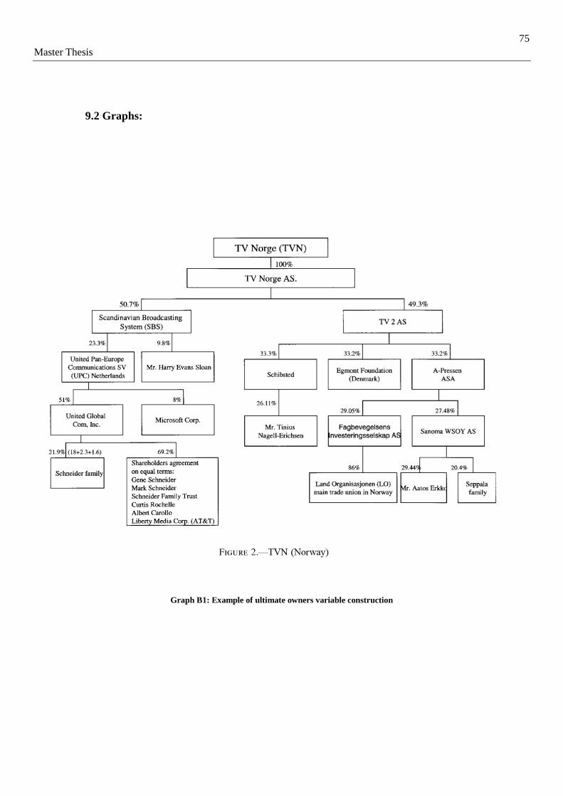
75

Master Thesis

9.2 Graphs:

Graph B1: Example of ultimate owners variable construction

76

Master Thesis

Graph B2: Civil Liberties Time Series

77

Master Thesis

Graph B3: Democracy Stability Time Series

78

Master Thesis

Graph B4: Executive System Time Series

79

Master Thesis

Graph B5: Imprisoned Journalists Time Series

80

Master Thesis

Graph B6: Majoritarian Rule Time Series

81

Master Thesis

Graph B7: Total Rents Time Series

82

Master Thesis

Graph B8: Murdered Journalists Time Series

83

Master Thesis

Graph B9: Structural differences between press and TV in terms of concentration (measured by HHI)

(Source: Noam‟s Book, 2016)

84

Master Thesis

Graph B10: Public ownership trend since the mid 2000’s

(Source: Noam‟s book, 2016)

85

Master Thesis

Graph B11: Representation of the average CPI

86

Master Thesis

Graph B12: Graphics for the identification of outliers

87

Master Thesis

Graph B13: Representation of the contradicting effects at play in the relationship between public TV and corruption.

88

Master Thesis

10. References:

Abed, G. T., & Davoodi, H. R. (2002). Corruption, structural reforms, and economic performance in the

transition economies. In G. T. Abed, & S. Gupta (Eds.), Governance, corruption, & economic performance

(pp. 489–537). Washington, D.C.: International Monetary Fund, Publication Services.

Ades, Alberto, and Rafael Di Tella. 1999. "Rents, Competition, and Corruption." American Economic

Review, 89(4): 982-993.

Ahrend, Rudiger, Press Freedom, Human Capital and Corruption (February 2002). DELTA Working Paper

No. 2002-11.

Arellano, Manuel, et Stephen Bond. «Some Tests of Specification for Panel Data: Monte Carlo Evidence

and an Application to Employment Equations». Review of Economic Studies 58, no 2 (1991): 277 97.

Badinger, Harald and Nindl, Elisabeth, Globalisation and Corruption, Revisited (October 2014). The World

Economy, Vol. 37, Issue 10, pp. 1424-1440, 2014.

Belsley, D. A., Kuh, E. Welsch, R. E. (1980). Regression Diagnostics: Identifying influential data and

sources of collinearity. New York: John Wiley

Besley, Timothy, and Andrea Prat. 2006. "Handcuffs for the Grabbing Hand? Media Capture and

Government Accountability." American Economic Review, 96(3): 720-736.

Bollen, K. A., and Jackman, R. W. 1990. “Regression Diagnostics: An Expository Treatment of Outliers and

Influential Cases.” Modern Methods of Data Analysis, edited by Fox, J., and Long, J. S. Sage Publications.

Brunetti, Aymo, et Beatrice Weder. « A free press is bad news for corruption ». Journal of Public Economics

87, no 7 8 (2003): 1801 24.

C. Bjørnskov and A. Freytag (2016), „An offer you can't refuse: murdering journalists as an enforcement

mechanism of corrupt deals‟, Public Choice, 167 (3–4): 221–43.

Camaj, L. (2013). "The media‟s role in fighting corruption: Media effects on governmental accountability".

The International Journal of Press/Politics, 18, 21-42.

Chow, Gregory C. “Tests of Equality Between Sets of Coefficients in Two Linear Regressions.”

Econometrica, vol. 28, no. 3, 1960, pp. 591–605.

Chowdhury, Shyamal K. "The effect of democracy and press freedom on corruption: an empirical test."

Economics letters 85.1 (2004): 93-101.

Coase, R. H. "British Broadcasting; A Study in Monopoly". Cambridge, Mass.: Harvard University Press,

1950.

Committee to Protect Journalists (CPJ), CPJ Reports, CPJ 2017

Cook, R. Dennis. "Detection of Influential Observation in Linear Regression." Technometrics 19, no. 1

(1977): 15-18.

89

Master Thesis

Djankov, Simeon, Caralee McLiesh, Tatiana Nenova, et Andrei Shleifer. « Who Owns the Media? » The

Journal of Law and Economics 46, no 2 (1 octobre 2003): 341 82.

Donchev, D. and Ujhelyi, G. (2014), What Do Corruption Indices Measure?. Economics & Politics,

26: 309–331.

Driscoll, J. C., and A. C. Kraay. 1998. "Consistent Covariance Matrix Estimation with Spatially Dependent

Panel Data". Review of Economics and Statistics 80: 549–560.

Eisenstadt, S. N. Traditional Patrimonialism and Modern Neopatrimonialism. Beverly Hills [Calif.]: Sage

Publications, 1973.

Frechette, G. R. (2006). A Panel Data Analysis of the Time-Varying Determinants of Corruption. CIRANO

Working Paper No 28 New York: New York University.

Freedom House,“Freedomhouse.org: Freedom of the Press.” Freedomhouse.org: Home, 2017,

www.freedomhouse.org/template.cfm?page=16.

Freille, Sebastian, M. Emranul Haque, et Richard Kneller. « A contribution to the empirics of press freedom

and corruption ». European Journal of Political Economy 23, no 4 (2007): 838 62.

Graeff, P., et G. Mehlkop. « The impact of economic freedom on corruption: different patterns for rich and

poor countries ». European Journal of Political Economy 19, no 3 (2003): 605 20.

Greene, W.H. (1993): "Econometric Analysis". Englewood Cliffs, NJ: Prentice-Hall

Gupta, S. H. D., & Terme, R. A. (1998). “Does Corruption Affect Income Inequality and Poverty?” IMF

Working Paper 98/76. International Monetary Fund, Washington D.C.

Gupta, Sanjeev, Luiz de Mello, et Raju Sharan. « Corruption and military spending ». European Journal of

Political Economy 17, no 4 (2001): 749 77.

Hamada, K., & Takarada, Y. (2007). Profitable mergers in cournot and stackelberg markets: 80 percent

share rule revisited. Working Paper Series No. 79 Faculty of Economics, Niigata University

Herfindahl, Orris C. « Concentration in the Steel Industry. » University Microfilms, 1951.

Heritage Foundation (Washington, D.C.), and Wall Street Journal (Firm). 1995. The index of economic

freedom. Washington, D.C.: Heritage Foundation.

Hirschman, Albert O. « National power and the Structure of Foreign Trade » Berkeley, 1945

Holcombe, Randall, et Christopher Boudreaux. « Regulation and corruption ». Public Choice 164, no 1

(2015): 75 85.

Houston, Joel F. & Lin, Chen & Ma, Yue, 2011. "Media ownership, concentration and corruption in bank

lending," Journal of Financial Economics, Elsevier, vol. 100(2), pages 326-350

Lambsdorff, J. G. (2007). "The institutional economics of corruption and reform". Cambridge, UK:

Cambridge University Press.

90

Master Thesis

Lindstedt, Catharina, and Daniel Naurin. "Transparency Is Not Enough: Making Transparency Effective in

Reducing Corruption" International Political Science Review 31, no. 3 (2010): 301-22.

Lučić, Danilo, Mladen Radišić, et Dušan Dobromirov. « Causality between corruption and the level of

GDP ». Economic Research-Ekonomska Istraživanja 29, no 1 (1 janvier 2016): 360 79.

Mauro, P. (1995). Corruption and growth. Quarterly Journal of Economics, 109, 681–712.

Noam, Eli M., et The International Media Concentration Collaboration. Who Owns the World‟s Media?:

Media Concentration and Ownership around the World. 1 edition. Oxford ; New York: Oxford University

Press, 2016.

Paldam, M. (2001). “Corruption and religion”, Adding to the economic model. Kyklos, 54, 383–414.

Pigou, A. C. (1932) "The Economics of Welfare". London: Macmillan and Co.

Rose-Ackerman, S., 1999. Corruption and Government. Cambridge Univ. Press, Cambridge, UK

Rose-Ackerman, S., 2006, "International Handbook on the Economics of Corruption", Edward Elgar Edition

Sarwar, Saima, and Muhammad Khalid Pervaiz. "An empirical investigation between trade liberalization

and corruption: A panel data approach." (2013). Journal of Economics and Sustainable Development, Vol 4

No 3, 2013

Seldadyo, H. , De Haan, J. The determinants of corruption: A literature survey and new evidence. Paper

prepared at the 2006 EPCS conference, Turku, Finland, 20–23 April (2006)

Shleifer, A., Vishny, R.W., 1993. Corruption. Quarterly Journal of Economics 108, 599–617.

Spyridon Boikos, 2016. "Corruption, Public Expenditure and Human Capital Accumulation," Review of

Economic Analysis, Rimini Centre for Economic Analysis, vol. 8(1), pages 17-45

Tanzi, V., & Davoodi, H. (1997). Corruption, public investment and growth. IMF Working Paper No. 139.

Washington: International Monetary Fund.

Torrez, Jimmy. « The effect of openness on corruption ». The Journal of International Trade & Economic

Development 11, no 4 (1 janvier 2002)

Transparency International (2016). "Corruption Perceptions Index". Transparency International.

Treisman, D. (2000). The causes of corruption: A cross-national study. Journal of Public Economics, 76,

399–457.

Wei, S. J. (2000). How taxing is corruption on international investors? Review of Economics and Statistics,

82 1–11.

Wooldridge, J. M. 2002. "Econometric Analysis of Cross Section and Panel Data". Cambridge, MA: MIT

Press