correlation surprise - springer · pdf filecontrolling for volatility, we ﬁnd that periods...

Original Article

Correlation surpriseReceived (in revised form): 12th December 2013

Will Kinlawis Senior Managing Director and Head of Portfolio and Risk Management Research at State Street Associates and has been awardedthe CFA designation.

David Turkingtonis Managing Director in the Portfolio and Risk Management Research group at State Street Associates and has been awarded theCFA designation.

Correspondence: David Turkington, State Street Associates, 140 Mt. Auburn Street, Cambridge, Massachusetts 02138, USA

ABSTRACT Soon after Harry Markowitz published his landmark 1952 article on portfolioselection, the correlation coefficient assumed vital significance as a measure of diversifica-tion and an input to portfolio construction. However, investors typically overlook the poten-tial for correlation patterns to help predict subsequent return and risk. Kritzman and Li (2010)introduced what is perhaps the first measure to capture the degree of multivariate asset price‘unusualness’ through time. Their financial turbulence score spikes when asset prices‘behave in an uncharacteristic fashion, including extreme price moves, decoupling of corre-lated assets, and convergence of uncorrelated assets.’ We extend Kritzman and Li’s studyby disentangling the volatility and correlation components of turbulence to derive a measureof correlation surprise. We show how correlation surprise is orthogonal to volatility and presentempirical evidence that it contains incremental forward-looking information. On average, aftercontrolling for volatility, we find that periods characterized by correlation surprise lead tohigher risk and lower returns to risk premia than periods characterized by typical correlations.This result holds across many markets including US equities, European equities and foreignexchange. Our results corroborate the predictive capacity of turbulence and suggest that itsdecomposition may also prove fruitful in forecasting investment performance.Journal of Asset Management (2014) 14, 385–399. doi:10.1057/jam.2013.27;published online 9 January 2014

Keywords: correlation; turbulence; volatility; dislocation; risk management

The online version of this article is available Open Access

INTRODUCTIONSoon after Harry Markowitz published hislandmark 1952 article on portfolio selection,the correlation coefficient assumed vitalsignificance as a measure of diversificationand an input to portfolio construction. Morerecently, investors have come to recognize theimportance of correlation to a wide varietyof investment activities. Analysts have usedthe parameter to detect regime shifts, describe

markets as ‘risk-on/risk-off ’ and justify theunderperformance of stock pickers. Of course,to monitor the tangled web of relationshipsbetween assets can be daunting. To covera universe of 10 assets, one must track 45 pair-wise correlations. Kritzman and Li (2010)introduced what is perhaps the first measure tocapture the degree of correlation ‘unusualness’across a set of assets through time. Theirfinancial turbulence score spikes when asset

© 2014 Macmillan Publishers Ltd. 1470-8272 Journal of Asset Management Vol. 14, 6, 385–399

www.palgrave-journals.com/jam/

prices ‘behave in an uncharacteristic fashion,including extreme price moves, decouplingof correlated assets, and convergence ofuncorrelated assets’. For at least two reasons,this framework is well suited to the purposeof quantifying correlation surprises. First, itsummarizes in a single measure the collectiveunusualness of correlations across any universeof assets. Second, rather than identify whethercorrelations are high or low, it measures thedegree to which interactions depart from theirhistorical norms, whatever those may be.

In this article, we extend Kritzman andLi’s study by disentangling the volatility andcorrelation components of turbulence to derivea measure of correlation surprise. We alsoshow how correlation surprise is orthogonal tovolatility and present empirical evidence thatit contains incremental forward-lookinginformation. On average, after controlling forvolatility, we find that periods characterizedby correlation surprise lead to higher riskand lower returns to risk premia than periodscharacterized by typical correlations. Thisresult holds across many markets includingUS equities, European equities and foreignexchange. Our results corroborate thepredictive capacity of turbulence and suggestthat its decomposition may also prove fruitfulin forecasting investment performance.

This article is organized as follows. First,we review the methodology behind Kritzmanand Li’s financial turbulence measure, alsoknown as the Mahalanobis distance, andreview its empirical features. Next, we showhow to decompose turbulence to isolate thecontribution of correlation surprises. We thenpresent empirical evidence that correlationsurprises contain incremental informationabout future risk and return at both dailyand monthly frequencies.

THE MAHALANOBIS DISTANCEAS A MEASURE OF FINANCIALTURBULENCEUsing a formula originally developed byMahalanobis (1927, 1936) to categorize human

skulls and later employed by Chow et al (1999)to stress test portfolios for turbulent periods,Kritzman and Li (2010) define their financialturbulence statistic as a multivariate unusualnessscore. We adopt the same definition ofturbulence but simply divide by the numberof assets (which is constant through time) inorder to facilitate ease of interpretation insubsequent sections of this article:

dt ¼ yt - μð ÞΣ - 1 yt - μð Þ=n (1)

where

dt turbulence for a particular time periodt (scalar)

yt vector of asset returns for periodt (1 × n vector)

μ sample average vector of historicalreturns (1 × n vector)

Σ sample covariance matrix of historicalreturns (n × n matrix)

n number of assets in universe

This statistic, which can be thought ofas a multivariate z-score, measures thestatistical unusualness of a contemporaneouscross-section of asset returns relative to itshistorical distribution. It captures the extentto which the risk-adjusted magnitudes of thereturns differ from their historical means aswell as the extent to which their interactionis inconsistent with the historical correlationmatrix. Turbulence is different fromcross-sectional volatility, which measures thedispersion around the cross-sectional meanbut ignores the time series means.1 It isalso different from the rolling volatility ofa portfolio because it describes theunusualness of a particular day rather than thedispersion in returns over a period of time.

Empirically, turbulence has severalattractive features:

� It tends to spike during recognizableperiods of market stress that arecharacterized by heightened volatilityand correlation breakdowns.

Kinlaw and Turkington

386 © 2014 Macmillan Publishers Ltd. 1470-8272 Journal of Asset Management Vol. 14, 6, 385–399

� It is linked to investment performance;on average, returns to a wide variety riskpremia are significantly lower duringturbulent periods.2

� It is persistent. Turbulent episodes tendto cluster in time and do not subsideimmediately after they arise.

Taken together, the persistence ofturbulence and its link with returns suggestthat investors could enhance performance byde-risking when turbulence first strikes. Forexample, Kritzman and Li show how toimprove the performance of a foreignexchange carry strategy by reducing exposurewhen currency turbulence rises. In this article,we put the persistence of turbulence – and itsrelationship with subsequent return and risk –under the microscope by disentanglingcorrelation surprises from magnitude surprises.

ISOLATING CORRELATIONSURPRISESThe turbulence methodology is ideally suitedto detecting periods when the co-movementbetween assets differs from what we wouldexpect based on historical correlations. For agiven day, the turbulence score captures boththe average degree of unusualness in individualasset returns (magnitude surprise) and thedegree of unusualness in the interactionbetween each pair of assets (correlationsurprise). To disentangle these two componentsand isolate the degree of correlation surprise,we first compute the magnitude surprise.Magnitude surprise is equal to the turbulencescore, given in equation (1), where alloff-diagonal elements in the covariancematrix are set to zero.3 This ‘correlation-blind’turbulence measure captures magnitudesurprises, but ignores whether co-movementis typical or atypical. Next, we divide thestandard turbulence score – which includescorrelation effects – by the magnitude surprise.This ratio is the correlation surprise: theunusualness of interactions on a particularday relative to history.

A correlation surprise ratio greaterthan one is associated with correlationbreakdowns (that is, previously correlatedassets diverging and/or previously negativelycorrelated assets converging). A correlationsurprise ratio less than one is associated withrelatively typical correlation outcomes. Inother words, days characterized by lowcorrelation surprise are actually less unusualthan the magnitudes of the individualreturns alone would suggest. To review,we compute the following quantities tocalculate correlation surprise:

1. Magnitude surprise: a ‘correlation-blind’turbulence score in which all off-diagonalsin the covariance matrix are set to zero.

2. Turbulence score: the degree of statisticalunusualness across assets on a given day,as given in equation (1).

3. Correlation surprise: the ratio ofturbulence to magnitude surprise,using the above quantities (2) and (1),respectively.

Correlation surprise ¼ TurbulenceMagnitude surprise

(2)

To build intuition around the turbulenceand correlation surprise scores, let us startby considering a single asset, x. In thiscase, turbulence is simply equal to thesquared z-score of the asset return, as shownin equation (3). To simplify the formulas inthis section, we will assume (without loss ofgenerality) that the average value of allrelevant return streams are zero, and we willsimply denote the asset's current period returnobservation as x.

Turbulence for one asset ¼x σ2x� � - 1

x

¼ xσx

� �2

¼ z2x ð3Þ

It is impossible, by definition, for oneasset to exhibit any correlation surprise.If we consider two assets, we can thinkof turbulence as a multivariate z-score.

Correlation surprise

387© 2014 Macmillan Publishers Ltd. 1470-8272 Journal of Asset Management Vol. 14, 6, 385–399

Rather than normalizing only by thevariance of an asset, as in equation (3),turbulence now normalizes for the entirecovariance matrix of the assets, whichaccounts for their historical variancesand the correlation between them as shownin equation (4).

Turbulence for two assets

¼ ð x y Þ σ2x ρσxσy

ρσxσy σ2y

! - 1x

y

� �ð4Þ

By dividing turbulence by magnitudesurprise, we can express the correlationsurprise for two assets as shown inequation (5) (the derivation of this formulais provided in the Appendix). We see thatcorrelation surprise is expressed in terms ofnormalized asset z-scores and the historicalcorrelation, ρ. All units of magnitude cancelout in this formula.

Correlation surprise for two assets

¼ 11 - ρ2

� 1 -ρzxzy

12 ðz2x + z2yÞ

!ð5Þ

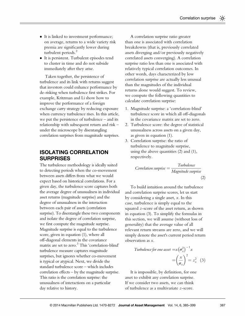
Turbulence and correlation surprise alsohave intuitive geometric interpretations.Consider a simple empirical example inwhich our universe consists of two assets,A and B, with means of zero, volatilitiesof 5 per cent, and a correlation of 0.5.Figure 1 shows the turbulence score,magnitude surprise and correlation surprisefor two multivariate return observations.

The dashed ellipse in Figure 1 is theiso-turbulence ellipse. All observations thatfall along this ellipse have the same turbulencescore. Its slant reflects the positive correlationbetween the two assets: in any given period, itis more likely that A and B move in the samedirection than in opposite directions. In otherwords, when A and B move in the samedirection, we require a larger returnmagnitude to produce the same degreeof turbulence. In this example, period 2is more turbulent than period 1 despitethe fact that the magnitudes of the two

observations are identical (each hasa magnitude surprise of 1.0). Period 2has a higher correlation surprise thanperiod 1 because it reflects an outcome wherethe two assets, which are expected to movetogether, diverge.

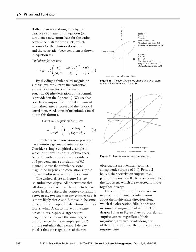
The correlation surprise score is akinto a compass: it contains informationabout the multivariate direction alongwhich the observation falls. It does notmeasure the magnitude of returns. Thediagonal lines in Figure 2 are iso-correlationsurprise vectors; regardless of theirmagnitude, any two points along oneof these lines will have the same correlationsurprise score.

Period 2A = +5%B = –5% Turbulence = 2.0Magnitude surprise = 1.0Correlation surprise = 2.0

Period 1A = +5%B = +5%Turbulence = 0.67Magnitude surprise = 1.0Correlation surprise = 0.67

Asset A return

Ass

et B

ret

urn

Iso-turbulence ellipse

Figure 1: The iso-turbulence ellipse and two returnobservations for assets A and B.

Asset A return

Iso-turbulence ellipse

Iso-correlation-surprise vector

Ass

et B

ret

urn

Figure 2: Iso-correlation surprise vectors.



HOW DOES CORRELATIONSURPRISE DIFFER FROMOTHER MEASURES THATINCORPORATECORRELATION?To our knowledge, correlation surprise is theonly measure that isolates the degree to whichthe co-movement across a set of assets istypical or atypical relative to history.4 Belowwe list three other measures that are sensitiveto correlation shifts and describe theimportant ways in which they fail to capturecorrelation surprises.

� Rolling correlation: Investors sometimesmonitor the rolling correlation betweentwo assets to help them identify regimeshifts. Whereas rolling correlation isa pair-wise measure, correlation surprisecan capture in a single parameter theunusualness of co-movement across a largeuniverse of assets.5 Indeed, the number ofpair-wise correlations quickly becomesunmanageable as the asset universeexpands. Again, to monitor a 10-assetuniverse, we would be required to estimate45 rolling correlations; for a 100-assetuniverse, the number increases to 4950.6

� Cross-sectional volatility: Cross-sectionalvolatility is different from correlationsurprise because it fails to account for thedegree to which a particular correlationoutcome is typical or atypical. Putdifferently, cross-sectional volatility spikeswhen asset returns diverge, regardlessof whether their typical correlation is10 per cent or 90 per cent. All else equal,a divergence is far more unusual in thelatter case than in the former.

� Multivariate Generalized AutoregressiveConditional Heteroskedasticity (GARCH)models: This class of models extends theunivariate GARCH framework to derivevolatility forecasts based on laggedcovariance terms as well as lagged varianceterms. For example, a multivariateGARCH model might forecast the

volatility of a two-stock portfolio based onlagged innovations in stock A, laggedinnovations in stock B and laggedcovariance terms between stocks A and B.7

Engle (2002) has proposed a DynamicConditional Correlation model, whichis a simple class of multivariate GARCHmodels. However, to our knowledge,none of the myriad multivariate GARCHspecifications account for interactionsbetween variance and covariance terms.8

And, as we will demonstrate in the nextsection, volatile episodes characterizedby atypical correlations tend to be morepersistent and severe than volatileepisodes characterized by typicalcorrelations. The decomposition of theMahalanobis distance enables us to analyzethe intertemporal relationship betweencorrelation and magnitude surprises ina way that multivariate GARCH modelsdo not.

DATA AND RESULTSWe construct correlation surprise series forthree asset universes: US equities, Europeanequities and currencies. Table 1 providesdetails regarding the component indices, startdate and lookback window for each series.

Figure 3 shows a scatter-plot of dailycorrelation surprise versus magnitude surprisescores for each asset universe. For thepurposes of this figure, we converted eachmetric into a per cent rank with regard to itsfull sample distribution. The dark lines showthe best fit linear regression line for each plot.

It is apparent from visual inspectionof Figure 3 that the correlation andmagnitude surprise scores capture differentinformation (which is collectively capturedin the turbulence score). In fact, ona contemporaneous basis the two metrics arenegatively correlated. What is intriguing isthat despite this contemporaneous negativecorrelation, we find strong empirical evidencethat high correlation surprise tends to precede



higher risk and also lower returns. We willdiscuss these findings in more detail shortly.Before we shift our focus to empirics, let usfirst consider a more theoretical question:why would we expect unusual correlations toprecede heightened volatility and lowerreturns? There are several plausible reasons.Investors who build correlation assumptionsinto their models – either explicitly orthrough intuition – may underperform whencorrelations deviate from their historical

norms, inducing them to de-risk. In addition,financial markets are not perfectly efficientand it takes some measure of time forinformation to propagate from one segmentto another. For example, consumer stocksmay react immediately to a particular newsitem, but financial stocks may not react untilinvestors have analyzed relationships betweenthese sectors, many of which are obscure andopaque. In this scenario, a shock wouldregister as a correlation event before it

0%

20%

40%

60%

80%

100%

0% 20% 40% 60% 80% 100%

U.S. Equities

0%

20%

40%

60%

80%

100%

0% 20% 40% 60% 80% 100%

European Equities

0%

20%

40%

60%

80%

100%

0% 20% 40% 60% 80% 100%

Currencies

Figure 3: Daily correlation surprise (vertical axis) versus magnitude surprise (horizontal axis).

Table 1: Time series data

US equities European equities Currencies

Lookback window 10 years of daily returnsa 10 years of daily returnsa 3 years of daily returnsIndex start date 26 November 1975 26 November 1975 24 November 1977Index end date 30 September 2010 30 September 2010 30 September 2010Data source S&P US Sectorsb MSCI Europe Sectorsb WMR 4 pm London Fix Rates

vs the US dollarConstituents used Consumer discretionary Consumer discretionary Australian dollarto build index Consumer staples Consumer staples British pound

Energy Energy Canadian dollarFinancials Financials Euroc

Healthcare Healthcare Japanese yenIndustrials Industrials New Zealand dollarInformation technology Information technology Norwegian kroneMaterials Materials Swedish kronaTelecommunications Telecommunications Swiss francUtilities Utilities —

aReturns are equally weighted to calculate mean and covariance. To capture longer cycles in the equity markets, webegin with a window of 3 years which is grown to 10 years and rolled forward.bDatastream sector data is used prior to 1995, when MSCI daily data becomes unavailable. The S&P 500® index andits GICS® level 1 sector sub-indices are proprietary to and are calculated, distributed and marketed by S&P Opco,LLC (a subsidiary of S&P Dow Jones Indices LLC) (‘SPDJI’), its affiliates and/or its licensors and have been licensedfor use. S&P®, S&P 500® and GICS®, among other famous marks, are registered trademarks of Standard & Poor’sFinancial Services LLC, and Dow Jones® is a registered trademark of Dow Jones Trademark Holdings LLC. NeitherSPDJI, its affiliates nor their third-party licensors make any representation or warranty, express or implied, as to theability of any index to accurately represent the asset class or market sector that it purports to represent. NeitherSPDJI, its affiliates nor their third-party licensors shall have any liability for any errors or omissions related to itsindices or the data included therein nor do the views and opinions of the authors expressed herein necessarily stateor reflect those of SPDJI, its affiliates and/or its licensors. SPDJI, its affiliates and their licensors reserve all rights withrespect to the S&P 500® index and its GICS® level 1 sector sub-indices.cDeutsche mark used prior to the introduction of the euro.



registers as a market-wide volatility event. It isalso possible that there is a behavioralexplanation. Perhaps investors tend to de-riskwhen markets are ‘acting weird’ and aredifficult to understand.

Whatever the reason, we find convincingempirical evidence that there is a lead-lagrelationship between correlation surprises,volatility and returns. For a vivid example ofhow correlation surprise manifests in practice,consider the month of September 2008, oneof the most turbulent months in financialhistory. A correlation surprise score above oneoccurred on nine days that month.9 Theaverage magnitude surprise score on the daysfollowing these correlation surprise eventswas 8.7, and the average daily S&P 500 returnwas −219 basis points (bps). In contrast, thedays with correlation surprise less than onewere followed by an average magnitudesurprise of 4.0 and an average S&P 500 returnof +86 bps. The worst one-day market lossduring the month occurred on 29 September,when the S&P 500 lost 879 bps from theprevious day’s close, accompanied by a verylarge magnitude surprise of 33. Correlationsurprise on the day of this drawdown was low(0.4), but on the previous day it was very high(1.9), in part because of a large divergence inthe daily return of the Materials sector (−252bps) and the Financials Sector (+309 bps),which over the preceding 10 years hadexperienced a positive correlation of 57 percent.10 A similar divergence occurred onFriday, 12 September, with correlationsurprise of 1.7 reflecting a gain for Materials(+323 bps) and a loss for Financials(−106 bps). The market dropped 471 bps onMonday, following news of Lehman’s default.

Monday had low correlation surprise, and themarket rallied 175 bps on Tuesday. However,Tuesday’s correlation surprise was 2.0.The market dropped another 471 bps onWednesday. This example is clearly anecdotaland in choosing it we are guilty of selectionbias. However, we find that the sameintuition holds on average across threedifferent markets from the 1970s through2010. We will now turn to a more robustempirical analysis.

For each of our three universes, weperform a series of experiments consistingof three broad steps:

1. Identify the 20 per cent of days in thehistorical sample with the highestmagnitude surprise scores.11

2. Partition the sample from step 1 into twosmaller subsamples: days with highcorrelation surprise (greater than one) anddays with low correlation surprise (lessthan one).

3. Measure, for the full sample identified instep 1 and its two subsamples identified instep 2, the subsequent volatility andperformance of relevant investments andstrategies.

Before presenting out-of-sample results,we examine the contemporaneousrelationship between magnitude surpriseand correlation surprise. Table 2 shows theaverage magnitude surprise for each ofthe three subsamples described in steps 1through 3, above. Of the 20 per cent most‘volatile’ days in each universe (as determinedby magnitude surprise), the days characterizedby high correlation surprise exhibit lessmagnitude surprise on average than the days

Table 2: Conditional average magnitude surprise on the day of the reading

US equities European equities Currencies

Day of top 20% MS with CS ⩽1 4.6 4.0 3.6Day of top 20% MS (all observations) 3.9 4.0 3.5Day of top 20% MS with CS>1 2.6 2.8 3.0Difference in means (high CS minus low CS sample) −2.0 −1.2 −0.6Percentage increase (high CS vs low CS sample) −43% −29% −17%



characterized by low correlation surprise. Inother words, the days characterized by themost extreme volatility tended to exhibitmore ‘typical’ correlations.

Table 3 shows the same results for the dayafter the reading. Now, the pattern isreversed: for each universe, the dayscharacterized by the most extreme magnitudesurprise tended to be preceded by atypicalcorrelations. In other words, heightenedvolatility coupled with unusual correlationsforetells higher next-day volatility thanheightened volatility coupled with typicalcorrelations. The t-statistics and p-values inTable 3 reveal that these differences arestatistically significant at the 90 per cent level.

These results suggest that correlationsurprises contain incremental informationabout future volatility. However, mostinvestors are more interested in future returns.To evaluate the relationship betweencorrelation surprise and subsequent returns, weemploy the same three-step test. But instead ofmeasuring magnitude surprise, we measurereturn, standard deviation and hit rate for threeinvestable indices. (Hit rate is defined as thepercentage of days following the given signalthat experience positive returns.) For US andEuropean equities, we analyze the return ofthe corresponding index listed in Table 1. Forcurrencies, we analyze the returns of a simplecarry strategy.12 Table 4 presents these results,along with the number of observations (days)in each subsample.

For all three investable indices, Table 4shows that the average return is lowerfollowing extreme magnitude dayscharacterized by high correlation surprise

than following extreme magnitude dayscharacterized by low correlation surprise.These results are statistically significantat the 95 per cent level for US equities.Interestingly, magnitude surprise alone is notparticularly effective for partitioning the nextday’s returns. In fact, for US equities, the20 per cent of days with the largest magnitudesurprise scores actually foretold higher returns,on average, than the remaining 80 per cent ofthe sample. Table 4 also reveals that the hitrate (per cent of positive days) for all threeindices is lowest following days characterizedby both high correlation surprise and highmagnitude surprise.13 Finally, Table 4 showsthat the standard deviation of returns is higherfollowing days where both magnitudesurprise and correlation surprise are high.14

This result holds for all three asset classes.To further explore the relationship

between correlation surprise and volatility,we analyze the performance of a hypotheticalshort volatility strategy. Specifically, wesimulate selling an at-the-money straddle:simultaneously writing an at-the-money putoption and an at-the-money call option.If the price of the reference asset remainsunchanged, then the options expire worthlessand the seller pockets the premium. But thisstrategy can suffer spectacular losses whenvolatility spikes and one of the options expiresin the money. Table 5 shows next-dayperformance of short volatility strategies inthe US equity, European equity and currencymarkets. Strictly speaking, these shortvolatility proxies are not investable becausetheir performance is approximated usingthe Black-Scholes-Merton model (based on

Table 3: Conditional average magnitude surprise on the day after the reading

US Equities European Equities Currencies

Day following top 20% MS with CS⩽ 1 2.1 2.1 1.5Day following top 20% MS (all observations) 2.3 2.4 1.7Day following top 20% MS with CS> 1 2.6 3.0 2.1Difference in means (high CS minus low CS sample) 0.5 0.9 0.6Percentage increase (high CS vs low CS sample) 21% 41% 38%t-statistic of difference in means test 1.54 3.12 3.02p-value of difference in means test 0.06 0.00 0.00



at-the-money implied volatility) as opposedto market prices for options. But theynonetheless provide insight into therelationship between correlation surprise andthe short volatility premium.

Table 5 reveals that the average annualizedreturn for all three strategies was lowestfollowing the subsample characterized byhigh magnitude surprise and high correlationsurprise simultaneously. The volatility washighest following this subsample. The hit rate(per cent of days with a positive return) waslowest following the joint occurrence in thecurrency market but highest in the two equitymarkets, where the signal appears to sufferfrom some false positives. Nonetheless,overall, these results suggest that a short

volatility investor would be well advised tohedge his or her exposure when magnitudesurprise and correlation surprise spikesimultaneously.

HOW QUICKLY DOES THESIGNAL DECAY?Thus far, our analysis has focused on therelationship between magnitude andcorrelation surprise on one day andperformance on the next. An investor wouldneed to react very quickly to exploit thisinformation. Table 6 presents an analysis ofhow quickly a one-day spike in the signaldecays. Specifically, for the experimentssummarized in Tables 4 and 5, we report the

Table 4: Investment performance on the day after the readinga

Average(annualized)

Std. deviation(annualized)

(%)

Hit rate(% dayspositive)

Numberof days

insample

US equities,S&P 500b

Full sample 7.2% 17.1 51.0 9092Day following top 20%MS with CS⩽1 27.7% 23.8 57.3 1211Day following top 20% MS(all observations)

16.2% 24.5 54.3 1818

Day following top 20%MS with CS>1 −6.7% 25.9 48.1 607Difference (high CS minus low CSsample)

−34.5% 2.2 −9.2 —

t-statistic of difference in means test −1.73 — — —

p-value of difference in means test 0.04 — — —

Europeanequities,MSCIEuropeb

Full sample 11.5% 16.1 55.0 9092Day following top 20%MS with CS⩽1 7.0% 21.2 54.0 1297Day following top 20% MS(all observations)

5.8% 22.9 53.3 1819

Day following top 20%MS with CS>1 2.5% 26.7 51.5 522Difference (high CS minus low CSsample)

−4.5% 5.5 −2.5 —



Currencies,G10 carrystrategyb

Full sample 3.4% 6.1 54.9 5024Day following top 20%MS with CS⩽1 −1.2% 6.9 54.6 784Day following top 20% MS(all observations)

−3.1% 7.8 53.7 1063

Day following top 20%MS with CS>1 −8.3% 10.0 51.3 279Difference (high CS minus low CSsample)

−7.0% 3.1 −3.3 —



aWe present annualized values for ease of interpretation. We conduct all statistical tests using daily data. All resultsare out of sample. However, we selected the threshold for the 20% of days with the largest magnitude surprisebased on the full sample. Choosing other volatility thresholds yielded similar results.bS&P 500 and MSCI Europe results from Nov 1975 to Sep 2010, currencies from Oct 1990 to Dec 2009.



following values for the subsequent 20-dayperiods:

� average magnitude surprise for periodsfollowing high correlation surprise minusaverage magnitude surprise for periodsfollowing low correlation surprise, and

� average return during periods followinghigh correlation surprise minus averagereturn during periods following lowcorrelation surprise.

We report average differentials for directexposure to the equity indices and G10 carrystrategy as well as to the simulated short-volatility strategies.

To better understand Table 6, consider theexample of US equities. The average

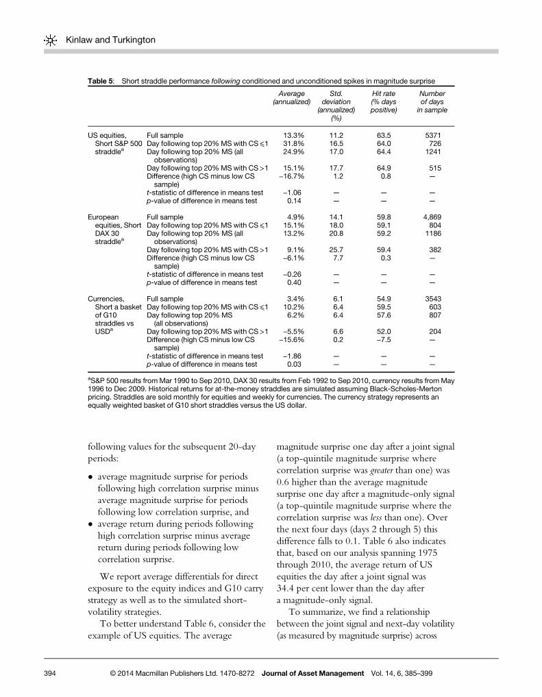
magnitude surprise one day after a joint signal(a top-quintile magnitude surprise wherecorrelation surprise was greater than one) was0.6 higher than the average magnitudesurprise one day after a magnitude-only signal(a top-quintile magnitude surprise where thecorrelation surprise was less than one). Overthe next four days (days 2 through 5) thisdifference falls to 0.1. Table 6 also indicatesthat, based on our analysis spanning 1975through 2010, the average return of USequities the day after a joint signal was34.4 per cent lower than the day aftera magnitude-only signal.

To summarize, we find a relationshipbetween the joint signal and next-day volatility(as measured by magnitude surprise) across

Table 5: Short straddle performance following conditioned and unconditioned spikes in magnitude surprise

Average(annualized)

Std.deviation

(annualized)(%)

Hit rate(% dayspositive)

Numberof days

in sample

US equities,Short S&P 500straddlea

Full sample 13.3% 11.2 63.5 5371Day following top 20%MS with CS⩽1 31.8% 16.5 64.0 726Day following top 20% MS (all

observations)24.9% 17.0 64.4 1241

Day following top 20%MS with CS>1 15.1% 17.7 64.9 515Difference (high CS minus low CS

sample)−16.7% 1.2 0.8 —



Europeanequities, ShortDAX 30straddlea

Full sample 4.9% 14.1 59.8 4,869Day following top 20%MS with CS⩽1 15.1% 18.0 59.1 804Day following top 20% MS (all

observations)13.2% 20.8 59.2 1186

Day following top 20%MS with CS>1 9.1% 25.7 59.4 382Difference (high CS minus low CS

sample)−6.1% 7.7 0.3 —



Currencies,Short a basketof G10straddles vsUSDa

Full sample 3.4% 6.1 54.9 3543Day following top 20%MS with CS⩽1 10.2% 6.4 59.5 603Day following top 20% MS

(all observations)6.2% 6.4 57.6 807

Day following top 20%MS with CS>1 −5.5% 6.6 52.0 204Difference (high CS minus low CS

sample)−15.6% 0.2 −7.5 —



aS&P 500 results fromMar 1990 to Sep 2010, DAX 30 results from Feb 1992 to Sep 2010, currency results fromMay1996 to Dec 2009. Historical returns for at-the-money straddles are simulated assuming Black-Scholes-Mertonpricing. Straddles are sold monthly for equities and weekly for currencies. The currency strategy represents anequally weighted basket of G10 short straddles versus the US dollar.



all three markets. We also find a relationshipbetween the joint signal and next-day returns.Of the three asset classes we studied, both ofthese relationships appear to decay most quicklyin the US equity market. For the short volatilitystrategies, the results are most persistent inthe currency market. In the next section, weexplore a way to derive correlation surprisesignals that apply to longer holding periods.

LONGER HORIZON SIGNALSSo far, we have viewed correlation surprise ona daily frequency. However, not all investorshave the ability to react so quickly to changesin the market environment. Investors whohave the ability to reallocate assets on a lessfrequent basis – such as monthly – can gaininformation from longer-term trends inmagnitude surprise and correlation surprise.We create monthly signals by aggregating thedaily time series within each month. Formagnitude surprise, we equally weightall the daily observations within eachmonth. For correlation surprise, however,we do not expect all observations to beequally informative. For example, if assets

only move by a few basis points on a givenday, their pattern of co-movement maynot reflect much more than random noise.But if assets move significantly, their patternof co-movement is much more likely torepresent an important fracture in themarket. Therefore, we compute a weightedaverage of correlation surprise for each monthusing the daily magnitude surprise scoresas weights. Mathematically, we calculatethe following quantities each month, whereT represents the total number of observations,MS is daily magnitude surprise and CS is dailycorrelation surprise:

MonthMSt ¼ 1T

XTi¼1

MSj

MonthCSt ¼PT

i¼1 CSiMSiPTj¼1MSj

Across all asset classes in our study, themonthly correlation surprise series isnegatively correlated to the moving averagemagnitude surprise series. Using thesemonthly signals, we repeat the conditionalreturns analysis from Tables 4 and 5 for

Table 6: Time decaya

After event, statistics for the following … …1 day … days 2–5 …days 6–10 …days 11–20

US equities Average magnitude surprise 0.6 0.1 0.1 0.2(0.06) (0.29) (0.23) (0.02)

S&P 500 return (%, ann) −34.5% 4.4% −1.5% −0.9%(0.04) (0.3) (0.42) (0.43)

S&P 500 short straddle return (%, ann) −16.7% −1.8% −1.7% −1.1%(0.14) (0.39) (0.38) (0.38)

European equities Average magnitude surprise 0.9 0.4 0.4 0.3(0) (0.02) (0.01) (0.02)

MSCI Europe return (%, ann) −4.5% −2.1% 2.1% −8.6%(0.41) (0.41) (0.4) (0.05)

DAX 30 short straddle return (%, ann) −6.1% −3.0% −5.8% 0.8%(0.4) (0.38) (0.24) (0.44)

Currencies Average magnitude surprise 0.6 0.4 0.2 0.1(0) (0) (0.01) (0.03)

G10 carry return (%, ann) −7.0% −0.2% −5.3% −4.3%(0.26) (0.49) (0.11) (0.05)

G10 short straddles return (%, ann) −15.6% −7.1% 0.1% −0.8%(0.03) (0.07) (0.49) (0.38)

p-values for difference-in-means tests shown in parentheses.aTime periods differ for each test. Please refer to the notes in Table 4 and Table 5 for specific dates.



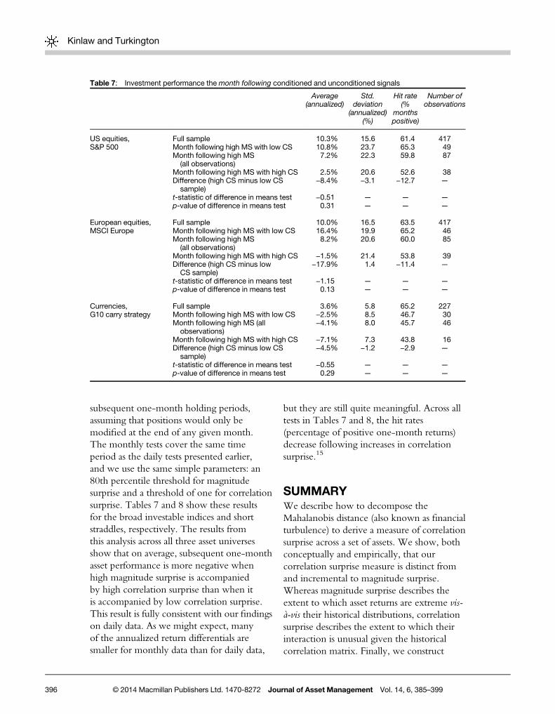
subsequent one-month holding periods,assuming that positions would only bemodified at the end of any given month.The monthly tests cover the same timeperiod as the daily tests presented earlier,and we use the same simple parameters: an80th percentile threshold for magnitudesurprise and a threshold of one for correlationsurprise. Tables 7 and 8 show these resultsfor the broad investable indices and shortstraddles, respectively. The results fromthis analysis across all three asset universesshow that on average, subsequent one-monthasset performance is more negative whenhigh magnitude surprise is accompaniedby high correlation surprise than when itis accompanied by low correlation surprise.This result is fully consistent with our findingson daily data. As we might expect, manyof the annualized return differentials aresmaller for monthly data than for daily data,

but they are still quite meaningful. Across alltests in Tables 7 and 8, the hit rates(percentage of positive one-month returns)decrease following increases in correlationsurprise.15

SUMMARYWe describe how to decompose theMahalanobis distance (also known as financialturbulence) to derive a measure of correlationsurprise across a set of assets. We show, bothconceptually and empirically, that ourcorrelation surprise measure is distinct fromand incremental to magnitude surprise.Whereas magnitude surprise describes theextent to which asset returns are extreme vis-à-vis their historical distributions, correlationsurprise describes the extent to which theirinteraction is unusual given the historicalcorrelation matrix. Finally, we construct

Table 7: Investment performance the month following conditioned and unconditioned signals

Average(annualized)

Std.deviation

(annualized)(%)

Hit rate(%

monthspositive)

Number ofobservations

US equities, Full sample 10.3% 15.6 61.4 417S&P 500 Month following high MS with low CS 10.8% 23.7 65.3 49

Month following high MS(all observations)

7.2% 22.3 59.8 87

Month following high MS with high CS 2.5% 20.6 52.6 38Difference (high CS minus low CS

sample)−8.4% −3.1 −12.7 —



European equities, Full sample 10.0% 16.5 63.5 417MSCI Europe Month following high MS with low CS 16.4% 19.9 65.2 46

Month following high MS(all observations)

8.2% 20.6 60.0 85

Month following high MS with high CS −1.5% 21.4 53.8 39Difference (high CS minus low

CS sample)−17.9% 1.4 −11.4 —



Currencies, Full sample 3.6% 5.8 65.2 227G10 carry strategy Month following high MS with low CS −2.5% 8.5 46.7 30

Month following high MS (allobservations)

−4.1% 8.0 45.7 46

Month following high MS with high CS −7.1% 7.3 43.8 16Difference (high CS minus low CS

sample)−4.5% −1.2 −2.9 —





Table 8: Short straddle performance the month following conditioned and unconditioned signals

Average(annualized)

Std. deviation(annualized)

(%)

Hit rate(% months positive)

Number ofobservations

US equities, Full sample 12.6% 8.7 73.6 246Short S&P 500 straddle Month following high MS with low CS 13.1% 13.8 77.1 35

Month following high MS (all observations) 11.3% 12.2 72.5 69Month following high MS with high CS 9.5% 10.5 67.6 34Difference (high CS minus low CS sample) −3.6% −3.3 −9.5 —



European equities, Full sample 5.9% 12.7 62.8 223Short DAX 30 straddle Month following high MS with low CS 30.6% 17.1 90.3 31

Month following high MS (all observations) 16.4% 15.5 72.3 65Month following high MS with high CS 3.4% 13.1 55.9 34Difference (high CS minus low CS sample) −27.1% −4.0 −34.4 —



Currencies, Full sample 4.0% 4.3 60.6 160Short a basket of G10 Month following high MS with low CS 8.0% 6.1 69.6 23straddles vs USD Month following high MS (all observations) 7.4% 5.9 69.4 36

Month following high MS with high CS 6.6% 5.6 69.2 13Difference (high CS minus low CS sample) −1.4% −0.5 −0.3 —



Correlation

surprise

397©

2014Macm

illanPub

lishersLtd

.1470-8272Jo

urnalofA

ssetManag

ement

Vol.14,6,385

–399

correlation surprise series for three differentasset classes and present evidence that the jointoccurrence of high magnitude surprise andhigh correlation surprise foretells highervolatility and lower return than highmagnitude surprise in isolation.

These findings have several concreteinvestment implications. A superiorunderstanding of correlation surprises couldenhance trade execution algorithms, whichrely on correlation estimates to manageopportunity costs. In addition, risk managerscould improve their volatility forecasts byincorporating correlation surprises into theirmodels. And, perhaps most interestingly,portfolio managers may be able to enhancetheir performance by de-risking when theyobserve correlation surprises coupled withheightened volatility.

ACKNOWLEDGEMENTSThe authors thank Megan Czasonis, MarkKritzman and Chirag Patel for helpfulcomments and assistance.

NOTES1. Imagine a period where all assets experience a 50 per cent

loss. Turbulence would spike but cross-sectional volatilitywould be zero.

2. Examples include the equity risk premium, small cappremium, growth minus value, the FX carry trade andhedge fund returns.

3. It is also equal to the average squared z-score across theassets in our universe.

4. A wide variety of conventional risk measures incorporateboth volatility and correlation but differ from correlationsurprise in obvious ways. For example, the rolling standarddeviation of a portfolio does not necessarily capturecorrelation surprises among its components. Consider aportfolio that is allocated to two stocks with a historicalcorrelation of 0.75. Imagine that on a particular day, onestock realizes a 20 per cent gain while the other experiencesa 20 per cent loss. The returns offset one another perfectly,the portfolio’s return for the day is 0 per cent, and its rollingvolatility declines. In this case, volatility fails to capture anextremely unusual correlation outcome. Volatility-basedmetrics (such as value at risk) and volatility forecastingmodels (such as ARCH and GARCH) fail to capturecorrelation surprises in similar fashion.

5. Another difference between rolling correlation andcorrelation surprise is that the former is, as its name suggests,

a rolling measure whereas the latter is a normalized measureof unusualness over a discrete period. The relationshipbetween rolling correlation and correlation surprise isanalogous to the relationship between rolling volatilityand a z-score.

6. A correlation matrix of n assets contains ((n*n)−n)/2 distinctcorrelation coefficients.

7. Typically, innovation terms are equal to squared residualsand covariance terms are equal to the product of residuals.

8. Multivariate GARCH models suffer from the ‘curse ofdimensionality’ in that the number of covariance termsincreases nonlinearly with the number of assets. Theaddition of a variance-covariance interaction term wouldrender them even more unwieldy. Indeed, much of theexisting multivariate GARCH literature is dedicated toadaptations that restrict the number of parameters. For anice discussion on this subject, see Fengler and Herwartz(2008).

9. The days with a correlation surprise score above one were2, 3, 5, 10, 12, 16, 19, 24 and 26 September.

10. The worst daily return following a correlation surprisereading less than one was 9 September’s loss of 341 basispoints.

11. We compute magnitude surprise series using thecomponents and lookback windows listed in Table 3.We pre-condition the experiments on the 20 per centof days with the largest magnitude surprise to isolatethe correlation surprise signals that are likely to contain themost information; days characterized by high correlationsurprise but miniscule returns are most likely noise.

12. To compute the carry returns, we assume equal sized longor short forward positions in each G10 currency(rebalanced monthly) depending on the currencies’ interestrate differentials versus the US dollar.

13. The hit rate also provides information about false positives.For example, Table 4 indicates that, in the US equitymarket, we observed positive returns after a joint signal48.1 per cent of the time.

14. It should be noted that the subsample means aresignificantly different from one another; hence, ifwe were to compute these volatilities around the fullsample means we would expect to see even largerdifferences.

15. These results do not depend on month-end rebalancing.Although not reported, we obtained very similar resultsbased on overlapping monthly holding periods.

REFERENCESChow, G., Jacquier, E., Lowry, K. and Kritzman, M. (1999)

Optimal portfolios in good times and bad. Financial AnalystsJournal 55(3): 65–73.

Engle, R. (2002) Dynamic conditional correlation: A simpleclass of multivariate generalized autoregressive conditionalheteroskedasticity models. Journal of Business & EconomicStatistics 20(3): 339–350.

Fengler, M. and Herwartz, H. (2008) Multivariate volatilitymodels. In: W. Hardle, N. Hautsch and L. Overbeck (eds.)Applied Quantitative Finance. Berlin Heidelberg: Springer,pp. 313–326.

Kritzman, M. and Li, Y. (2010) Skulls, financial turbulence, andrisk management. Financial Analysts Journal 66(5): 30–41.



Mahalanobis, P.C. (1927) Analysis of race-mixture in Bengal.Journal of the Asiatic Society of Bengal 23: 301–333.

Mahalanobis, P.C. (1936) On the generalised distance instatistics. Proceedings of the National Institute of Sciencesof India 2(1): 49–55.

Markowitz, H. (1952) Portfolio selection. Journal of Finance7(1): 77–91.

APPENDIX

Correlation surprise mathematicsfor two assetsTo build intuition around the correlationsurprise methodology, we can investigate asimple two-asset example algebraically. Tosimplify the formulas, we will assume(without loss of generality) that the averagevalue of x and average value of y are bothzero.

CS ¼ TIMS

¼x yð Þ σ2x ρσxσy

ρσxσy σ2y

� � - 1xy

� �

x yð Þ σ2x 00 σ2y

� � - 1xy

� �

Using the matrix identity that

a bc d

� � - 1

¼ 1ad - bc

d - b- c a

� �

and multiplying out the matrices, we find that

CS ¼ σ2xσ2y

ð1 - ρ2Þσ2xσ2y´x2σ2y + y

2σ2x - 2xyρσxσyx2σ2y + y2σ2x

CS ¼ 11 - ρ2

´ 1 -2xyρσxσyx2σ2y + y2σ2x

!

CS ¼ 11 - ρ2

´ 1 -2ρ x

σxyσy

x2

σ2x+ y2

σ2y

0B@

1CA

CS ¼ 11 - ρ2

´ 1 -ρzxzy

12 ðz2x + z2yÞ

!

This formula highlights that correlationsurprise is a function of the assets’ correlationand their z-scores, which are volatility-normalized. All units expressing magnitudecancel out in the formula: the units ofz-scores in the numerator equal the units ofz-scores in the denominator. Hence, thecorrelation surprise score contains onlyinformation about the direction ofco-movement, analogous to a compass orradial coordinate.

For this algebraic example we candetermine that the minimum correlationsurprise for a given correlation ρ is (1−|ρ|)/(1−ρ2) and the maximum is (1+|ρ|)/(1−ρ2).If correlation is zero, the minimum andmaximum will both equal one. This makessense, because if we do not expect anystructured relationship between the twovariables, no observed pattern of co-movement will be any more or less unusualthan another. However, as the steady-statecorrelation intensifies, we will be increasinglyless surprised by co-movement that is alignedwith the steady-state correlation (we will see aCS score less than one), and increasingly moresurprised by co-movement that diverges fromthe steady-state correlation (we will see a CSscore greater than one).

This work is licensed under aCreative Commons Attribution

3.0 Unported License. To view a copy of thislicense, visit http://creativecommons.org/licenses/by/3.0/

Disclaimer: The views expressed in this article are the views solely of the authors and do notnecessarily represent the views of State Street Corporation.



correlation surprise - springer · pdf filecontrolling for volatility, we ﬁnd that periods...

Documents