correlation of nuclear gauge density and laboratory core density procedures

7/31/2019 Correlation of Nuclear Gauge Density and Laboratory Core Density Procedures

http://slidepdf.com/reader/full/correlation-of-nuclear-gauge-density-and-laboratory-core-density-procedures 1/13

STP 204-26

Standard Test Section: ASPHALT MIXES

Procedures Manual Subject: CORRELATION OF NUCLEAR GAUGE

DENSITY AND LABORATORY CORE DENSITY

1. SCOPE

1.1. Description of Test

The standard test procedure is used to correlate the density results of asphalt concrete

pavements obtained with a nuclear density gauge and with a laboratory test on a cored

sample.

1.2. Application of Test

This test is to be performed at the beginning of each paving contract for each lift, for

every change in lift thickness, for every change in the job mix formula and anytime there

is a substantial change in the material of the underlying layers to calibrate the density-in-

place by nuclear gauge (obtained by STP 204-6) with the density obtained from cored

samples. 2. APPARATUS AND MATERIALS

2.1. Equipment Required

A calculator and the form “BASIC WORKSHEET FOR LINEAR RELATIONSHIPS

BETWEEN TWO VARIABLES”. Alternatively a computer using Microsoft Windows,

Microsoft Excel and a disk containing the Microsoft Excel Workbook

“DENSCOR.XLS”.

A printer for hard copy records.

2.2. Data Required

Seven to ten random test locations where cores and nuclear density readings will be

taken. The test locations are to be determined by STP 107. The core diameter is 150

mm.

3. PROCEDURE

3.1. Test Procedure

Determine the sample locations using the procedure described in STP 107. Mark the

core/nuclear gauge sample locations.

Obtain density-in-place measurements with the nuclear gauge using the procedure

Date: 2003 05 30 Page: 1 of 13



Standard Test Procedures Manual STP 204-26

Section: ASPHALT MIXES Subject: CORRELATION OF NUCLEAR GAUGE DENSITY

AND LABORATORY CORE DENSITY

described in STP 204-6. Record the density measurement for each sample location as Xi.

Obtain a core, in the exact same location as the nuclear gauge density readings were

taken, using the procedure described in STP 204-5. Number this core with the samenumber that was used to record the in-place-density with the nuclear gauge. Determine

the core density in the laboratory. Record the core density for each sample as Yi.

Enter the results of Xi and Yi on the form “BASIC WORKSHEET FOR LINEAR

RELATIONSHIPS BETWEEN TWO VARIABLES”.

Complete the calculations on the form to determine:

• Are any of the samples outliers that should not be used.

• The linear regression coefficients “a” and “b” for the equation “y = b X + a”.

• The regression coefficient ( r =S

S S

xy

xx yy

).

• The tstatistic ( tr (n - 2)

(1-r statistic

2=

)

).

Compare the value of the tstatistic to the value of t(0.975) obtained from the Student’s t

Distribution Table for n-2 degrees of freedom and a 97.5% probability level.

• If the tstatistic is larger than t(0.975), there is a 97.5% chance that the correlation

coefficient (r) is significantly different from 0 (a correlation coefficient (r) of 0

indicates a complete absence of correlation and a correlation coefficient (r) of 1 or -1 indicates perfect correlation). This means that there is a statistically valid

correlation.

• If the tstatistic is smaller than t(0.975), there is a 97.5% chance that the correlation

coefficient (r) is not significantly different from zero. This means that there is not

a statistically valid correlation. Two additional random sample locations should

be determined. Cores and nuclear density readings should be obtained. The

correlation procedure should be repeated with the additional samples included.

Plot the sample data and the regression equation on the Correlation Chart to ensure that

the regression line has a good fit to the data and that the data is in fact linear. Check the

value of the standard error Syx. It should be relatively small (less than 1%) compared tothe value of in-place-density by nuclear gauge.

Alternatively enter the values for Xi and Yi into the Microsoft Excel Workbook

“DENSCOR.XLS”. The program will check for outliers, calculate all of the coefficients

and check for statistical validity.

of 13 Date: 2003 05 30




Section: ASPHALT MIXES Subject: CORRELATION OF NUCLEAR GAUGE


The regression line has the form “Y = b X + a”. Future values of density-in-place by

nuclear gauge (ρfuture) can be collected using STP 204-6. For any future density-in-place

by nuclear gauge reading, compute the correlated density using the formula:

Nuclear Densityadjusted = b (ρfuture) + a

4. RESULTS AND CALCULATIONS

4.1. Calculations

The procedure for correlating the in-place-density by nuclear gauge to laboratory core

densities can best be illustrated by an example.

4.1.1. Determine In-Place-Density by Nuclear Gauge and Laboratory Core Density

Assume that seven random test locations were determined by STP 107. The

locations were marked and the in-place-density was determined for each location

using STP 204-5. Each location was also cored. The in-place-density by nuclear

gauge was determined as shown below. The laboratory density was determined

for each core.

The in-place-density by nuclear gauge measurements were:

• Location 1: 2,237.1 kg/m3 • Location 5: 2,325.3 kg/m

3


3


3

• Location 4: 2,312.0 kg/m

3

The corresponding laboratory core density results were:


3


3


3

• Location 4: 2,285.0 kg/m3

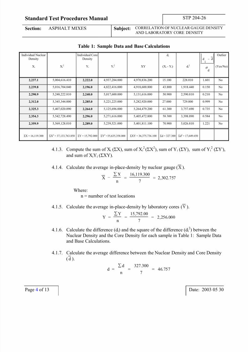
4.1.2. “BASIC WORKSHEET FOR LINEAR RELATIONSHIPS BETWEEN TWO

VARIABLES”

Enter the values of Xi and Yi in the table “BASIC WORKSHEET FOR LINEAR

RELATIONSHIPS BETWEEN TWO VARIABLES” and compute Xi2, Yi

2and

XY as illustrated in Table 1: Sample Data and Base Calculations.

Date: 2003 05 30 of 13






Table 1: Sample Data and Base Calculations

Individual Nuclear

Density

Xi Xi2

Individual Core

Density

Yi Yi2 XY

di

(Xi - Yi) di2

d

i

d

d

−

σ

Outlier

(Yes/No)

2,237.1 5,004,616.410 2,222.0 4,937,284.000 4,970,836.200 15.100 228.010 1.601 No

2,239.8 5,016,704.040 2,196.0 4,822,416.000 4,918,600.800 43.800 1,918.440 0.150 No

2,290.9 5,248,222.810 2,240.0 5,017,600.000 5,131,616.000 50.900 2,590.810 0.210 No

2,312.0 5,345,344.000 2,285.0 5,221,225.000 5,282,920.000 27.000 729.000 0.999 No

2,325.3 5,407,020.090 2,264.0 5,125,696.000 5,264,479.200 61.300 3,757.690 0.735 No

2,354.3 5,542,728.490 2,296.0 5,271,616.000 5,405,472.800 58.300 3,398.890 0.584 No

2,359.9 5,569,128.010 2,289.0 5,239,521.000 5,401,811.100 70.900 5,026.810 1.221 No

ΣX = 16,119.300 ΣX2 = 37,133,763.850 ΣY = 15,792.000 ΣY2 =35,635,358.000 ΣXY = 36,375,736.100 Σd = 327.300 Σd2 = 17,649.650

4.1.3. Compute the sum of Xi (ΣX), sum of Xi2 (ΣX

2), sum of Yi (ΣY), sum of Yi

2(ΣY2),

and sum of XiYi (ΣXY).

4.1.4. Calculate the average in-place-density by nuclear gauge ( X ).

X =X

n=

16,119.300

7= 2,302.757

∑

Where:

n = number of test locations

4.1.5. Calculate the average in-place-density by laboratory cores (Y ).

Y =Y

n=

15,792.00

7= 2,256.000

∑

4.1.6. Calculate the difference (di) and the square of the difference (di2) between the

Nuclear Density and the Core Density for each sample in Table 1: Sample Data

and Base Calculations.

4.1.7. Calculate the average difference between the Nuclear Density and Core Density

( d ).

d =d

n=

327.300

7= 46.757

∑

of 13 Date: 2003 05 30






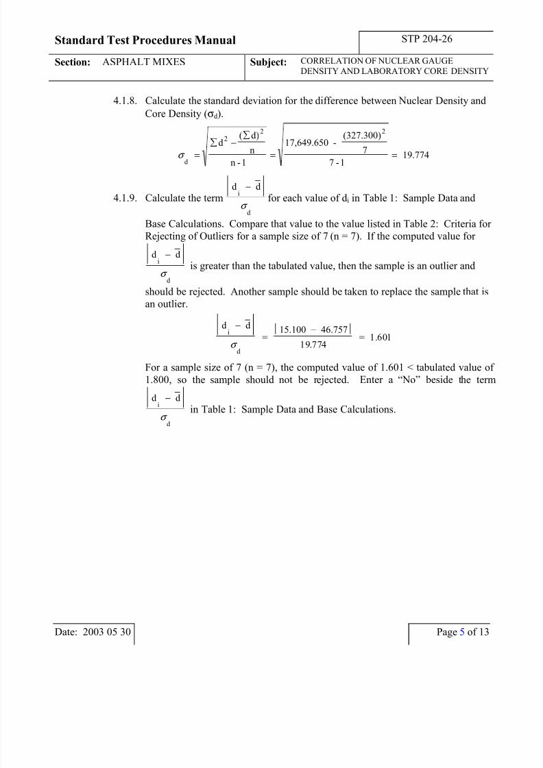
4.1.8. Calculate the standard deviation for the difference between Nuclear Density and

Core Density (σd).

σ d

2 2 2

d( d)

n

n -1

17,649.650 -(327.300)

7

7 -119.774=

∑ − ∑

= =

4.1.9. Calculate the termd d

i

d

−

σ

for each value of di in Table 1: Sample Data and

Base Calculations. Compare that value to the value listed in Table 2: Criteria for

Rejecting of Outliers for a sample size of 7 (n = 7). If the computed value for

d di

d

−

σ is greater than the tabulated value, then the sample is an outlier and

should be rejected. Another sample should be taken to replace the sample that is

an outlier.

d d

=15.100 46.757

= 1.601i

d

− −

σ 19 774.

For a sample size of 7 (n = 7), the computed value of 1.601 < tabulated value of

1.800, so the sample should not be rejected. Enter a “No” beside the term

d di

d

−

σ

in Table 1: Sample Data and Base Calculations.

Date: 2003 05 30 of 13






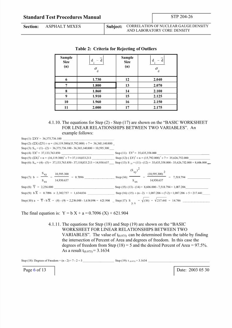
Table 2: Criteria for Rejecting of Outliers

SampleSize

(n)

d di

d

−

σ

SampleSize

(n)

d di

d

−

σ

6 1.730 12 2.040

7 1.800 13 2.070

8 1.860 14 2.100

9 1.910 15 2.125

10 1.960 16 2.150

11 2.000 17 2.175

4.1.10. The equations for Step (2) - Step (17) are shown on the “BASIC WORKSHEET

FOR LINEAR RELATIONSHIPS BETWEEN TWO VARIABLES”. An

example follows:Step (1): ΣXY = 36,375,736.100 __________________________________

Step (2): (ΣX) (ΣY) ÷ n = (16,119.300)(15,792.000) ÷ 7 = 36,365,140.800 _

Step (3): Sxy = (1) - (2) = 36,375,736.100 - 36,365,140.800 = 10,595.300 ___

Step (4): ΣX2 = 37,133,763.850 ___________________________________ Step (11): ΣY2 = 35,635,358.000 ___________________________________

Step (5): (ΣX)2 ÷ n = (16,119.300)2 ÷ 7 = 37,118,833.213 _______________ Step (12): (ΣY)2 ÷ n = (15,792.000)2 ÷ 7 = 35,626,752.000 ______________

Step (6): Sxx = (4) - (5) = 37,133,763.850 - 37,118,833.213 = 14,930.637 ___ Step (13): Syy = (11) - (12) = 35,635,358.000 - 35,626,752.000 = 8,606.000 _

Step (7): b =xyS

xxS=

10,595.300

14,930.637= 0.7096 ____________________ Step (14):

xy

(S2

xxS=

(10,595.300) 2

14,930.637= 7,518.794

)

_______________

Step (8): Y = 2,256.000 ________________________________________ Step (15): (13) - (14) = 8,606.000 - 7,518.794 = 1,087.206_______________

Step (9): b X = 0.7096 2,302.757 = 1,634.036× __________________ Step (16): (15) ÷ (n - 2) = 1,087.206÷ (7-2) = 1,087.206 ÷ 5 = 217.441_____

Step (10): a = Y - b X = (8) - (9) = 2,256.000 - 1,634.096 = 621.904 _ Step (17): Sy. x

= (16) = 217.441 = 14.746 __________________

The final equation is: Y = b X + a = 0.7096 (X) + 621.904

4.1.11. The equations for Step (18) and Step (19) are shown on the “BASIC

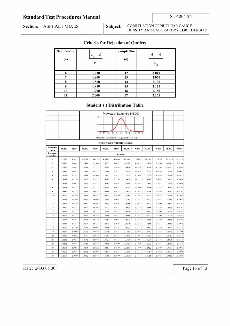
WORKSHEET FOR LINEAR RELATIONSHIPS BETWEEN TWOVARIABLES”. The value of t(0.975) can be determined from the table by finding

the intersection of Percent of Area and degrees of freedom. In this case the

degrees of freedom from Step (18) = 5 and the desired Percent of Area = 97.5%.

As a result t(0.975) = 3.1634.

Step (18): Degrees of Freedom = (n - 2) = 7 - 2 = 5 _____________________ Step (19): t(0.975) = 3.1634 _________________________________________

of 13 Date: 2003 05 30






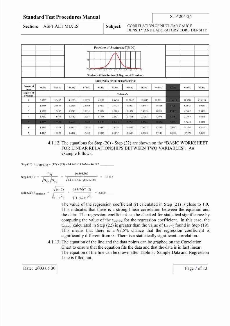
Student's t Distribution (5 Degrees of Freedom)

STUDENTS t DISTRIBUTION CURVE

Percent of

Area80.0% 82.5% 85.0% 87.5% 90.0% 92.5% 95.0% 96.0% 97.0% 97.5% 98.0% 99.0%

Degrees of

FreedomValues of t

1 3.0777 3.5457 4.1653 5.0273 6.3137 8.4490 12.7062 15.8945 21.2051 25.4519 31.8210 63.6559

2 1.8856 2.0645 2.2819 2.5560 2.9200 3.4428 4.3027 4.8487 5.6428 6.2054 6.9645 9.9250

3 1.6377 1.7692 1.9243 2.1131 2.3534 2.6808 3.1824 3.4819 3.8961 4.1765 4.5407 5.8408

4 1.5332 1.6465 1.7782 1.9357 2.1318 2.3921 2.7765 2.9985 3.2976 3.4954 3.7469 4.6041

5 1.4759 1.5798 1.6994 1.8409 2.0150 2.2423 2.5706 2.7565 3.0029 3.1634 3.3649 4.0321

6 1.4398 1.5379 1.6502 1.7822 1.9432 2.1510 2.4469 2.6122 2.8289 2.9687 3.1427 3.7074

7 1.4149 1.5092 1.6166 1.7422 1.8946 2.0897 2.3646 2.5168 2.7146 2.8412 2.9979 3.4995

Preview of Student's T(5.00)

0.0

0.2

0.4

0.0 1.2 2.4 3.5 4.7 5.9-1.2-2.4-3.5-4.7-5.9

4.1.12. The equations for Step (20) - Step (22) are shown on the “BASIC WORKSHEET

FOR LINEAR RELATIONSHIPS BETWEEN TWO VARIABLES”. An

example follows:

Step (20): Sy.x t(0.975) = (17) × (19) = 14.746 × 3.1634 = 46.647 _________

Step (21): r =xyS

xxS yyS

=10,595.300

14,930.637 8,606.000= 0.9347

Step (22): t statistic =r (n - 2)

(1 - r 2

=0.9347 (7 - 2)

(1- 0.93472

= 5.880

) )

_____

The value of the regression coefficient (r) calculated in Step (21) is close to 1.0.

This indicates that there is a strong linear correlation between the equation and

the data. The regression coefficient can be checked for statistical significance by

computing the value of the tstatistic for the regression coefficient. In this case, the

tstatistic calculated in Step (22) is greater than the value of t (0.975) found in Step (19).

This means that there is a 97.5% chance that the regression coefficient is

significantly different from 0. There is a statistically significant correlation.

4.1.13. The equation of the line and the data points can be graphed on the Correlation

Chart to ensure that the equation fits the data and that the data is in fact linear.

The equation of the line can be drawn after Table 3: Sample Data and Regression

Line is filled out.

Date: 2003 05 30 of 13






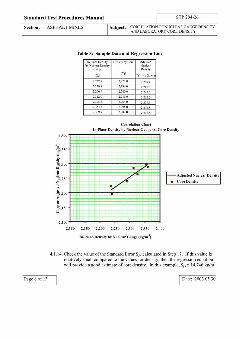
Table 3: Sample Data and Regression Line

In Place Density

by Nuclear Density

Gauge

(Xi)

Density by Core

(Yi)

Adjusted

Nuclear

Density

( $Y i = b Xi + a)

2,237.1 2,222.0 2,209.4

2,239.8 2,196.0 2,211.3

2,290.9 2,240.0 2,247.5

2,312.0 2,285.0 2,262.5

2,325.3 2,264.0 2,271.9

2,354.3 2,296.0 2,292.5

2,359.9 2,289.0 2,296.5

Correlation Chart

In-Place-Density by Nuclear Gauge vs. Core Density

2,100

2,150

2,200

2,250

2,300

2,350

2,400

2,100 2,150 2,200 2,250 2,300 2,350 2,400

In-Place-Density by Nuclear Gauge (kg/m

3

)

C o r e o r A d j u s t e d N u c

l e a r D e n s i t y ( k g / m 3 )

Adjusted Nuclear Density

Core Density

4.1.14. Check the value of the Standard Error Syx calculated in Step 17. If this value is

relatively small compared to the values for density, then the regression equation

will provide a good estimate of core density. In this example, Syx = 14.746 kg/m3

of 13 Date: 2003 05 30






is relatively small (< 1.0%) compared to the in-place nuclear density values of

2,200-2,360 kg/m3, so it should provide a good estimate of the core density.

4.1.15. Once the correlation has been completed the equation is used to adjust in-place-

density by nuclear gauge readings. If a nuclear density reading of 2,250.0 kg/m3

was obtained, the adjusted density would be computed using the equation:

Y = Adjusted Nuclear Density

= b (X) + a

= 0.7096 (X) + 621.904

= 0.7096 (2,250.0 kg/m3) + 621.904

= 2,218.5 kg/m3

The value of 2,218.5 kg/m3

would be used to determine acceptance.

4.2. Reporting Results

The Department will develop the regression equation to be used for correcting the

nuclear density gauge readings.

5. CALIBRATIONS, CORRECTIONS, REPEATABILITY

5.1. Tolerances and Repeatability

The correlation coefficient (r) is an index of the degree of correlation between the data.

The size of the correlation coefficient (r) is an indication of the degree of relationship

between two variables. A high value of the correlation coefficient (r), i.e. close to 1 or -1, merely indicates a close straight line relationship between the two variables. It does

not mean that one caused the other. Values of the correlation coefficient (r) equal to 1 or

-1 indicate perfect correlation and values of the correlation coefficient (r) equal to 0

indicate the complete absence of linear correlation.

If the relationship line is based on a relatively small number of points, in our case 7

points, the value of the correlation coefficient may be due to chance variations in

sampling and errors of measurement. The value of the regression coefficient should be

checked for statistical significance by computing the tstatistic. and comparing it with the t

value at a 97.5 % probability level (t(0.975)) (and the appropriate degrees of freedom). If

the tstatistic is greater than the value of t(0.975) then there is a 97.5% chance that the

correlation coefficient (r) is significantly different than 0 and there is a correlation

between the two variables.

The standard error of the estimate (Sy.x) gives an indication of the error associated with the

regression line. In the previous example, the standard error is 14.746 kg/m3. The value

of Sy.x is of practical importance because it gives an indication of the reliability of the

Date: 2003 05 30 of 13






equation. If the value of Sy.x is relatively small (<1.0%), compared to the values of the in-

place-density by nuclear gauge, and the regression coefficient is statistically significant,

the equation will provide a good estimate of the density that would have been obtained

by coring.

5.2. Sources of Error

Possible sources of error include those listed in STP 204-6 and STP 204-5.

6. ADDED INFORMATION

6.1. References

References are STP 204-5, STP 204-6 and the owner’s manual for the nuclear gauge.

6.2. Sample Retention

Samples should be retained according to the procedures laid out in STP 204-5.

Correlation worksheets and equations should be retained as part of the contract

documents.

6.3. Protection of Samples

The core samples should be protected according to the procedures set out in STP 204-5.

6.4. Proper Sample Identification

It is vital to ensure that the samples are identified so that the in-place-density by nuclear gauge corresponds to the laboratory core density for the same sample location.

6.5. Safety

The current safety regulations are to be followed as outlined in the Traffic control

Devices Manual For Work zones and the Safety Manual.

of 13 Date: 2003 05 30






Project:__________________________________________

Date: ___________________________________________

By: _____________________________________________

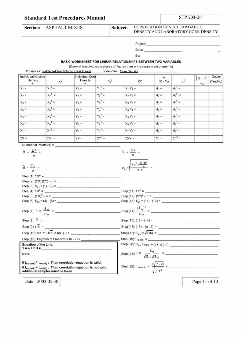
BASIC WORKSHEET FOR LINEAR RELATIONSHIPS BETWEEN TWO VARIABLES

(Carry at least two more places of figures than in the single measurements)

X denotes: In-Place-Density by Nuclear Gauge______ Y denotes: Core Density ______________________

Individual Nuclear Density

XXi

2

Individual CoreDensity

YYi

2 XY

di

(Xi - Yi) di2

d di

d

−

σ

Outlier

(Yes/No)

X1 = X12 = Y1 = Y1

2 = X1 Y1 = d1 = d12 =

X2 = X22 = Y2 = Y2

2 = X2 Y2 = d2 = d22 =

X3 = X32 = Y3 = Y3

2 = X3 Y3 = d3 = d32 =

X4 = X42 = Y4 = Y4

2 = X4 Y4 = d4 = d42 =

X5 = X52 = Y5 = Y5

2 = X5 Y5 = d5 = d52 =

X6 = X62 = Y6 = Y6

2 = X6 Y6 = d6 = d62 =

X7 = X72 = Y7 = Y7

2 = X7 Y7 = d7 = d72 =

ΣX = ΣX2 = ΣY = ΣY2 = ΣXY = Σd = Σd2

=

Number of Points (n) = _____________________________________

X =X

n

∑= _____________________________________________ Y =

Y

n

∑= _____________________________________________

d =d

n

∑= _____________________________________________ σ d

d( d)

nn -1

22

=∑ −

∑

= ______________________________________

Step (1): ΣXY = ___________________________________________

Step (2): (ΣX) (ΣY) ÷ n = ____________________________________

Step (3): Sxy = (1) - (2) = ____________________________________

Step (4): ΣX2 = ___________________________________________ Step (11): ΣY2 = __________________________________________

Step (5): (ΣX)2 ÷ n = _______________________________________ Step (12): (ΣY)2 ÷ n = ______________________________________

Step (6): Sxx = (4) - (5) = ____________________________________ Step (13): Syy = (11) - (12) = _________________________________

Step (7): b =S

S

xy

xx

= _____________________________________ Step (14):xy

2

xx

(S

S

)= _______________________________________

Step (8): Y = ____________________________________________ Step (15): (13) - (14) = _____________________________________

Step (9): b X = ___________________________________________ Step (16): (15) ÷ (n - 2) = ___________________________________

Step (10): a = Y - b X = (8) -(9) = ____________________________ Step (17): Sy.x = (16) = ___________________________________

Step (18): Degrees of Freedom = (n - 2) = ______________________ Step (19): t(0.975) = _________________________________________ Equation of the Line:

Y = a + b X = ________________________________________

Note:

If tstatistic t(0.975) : Then correlation equation is valid.

If tstatistic < t(0.975) : Then correlation equation is not valid,

additional samples must be taken

Step (20): Sy.x t(0.975) = (17) × (19) ___________________________

Step (21): r = = ______________________________ S

S S

xy

xx yy

Step (22): t =r (n - 2)

(1-r

statistic2 )

= ____________________________

Date: 2003 05 30 of 13






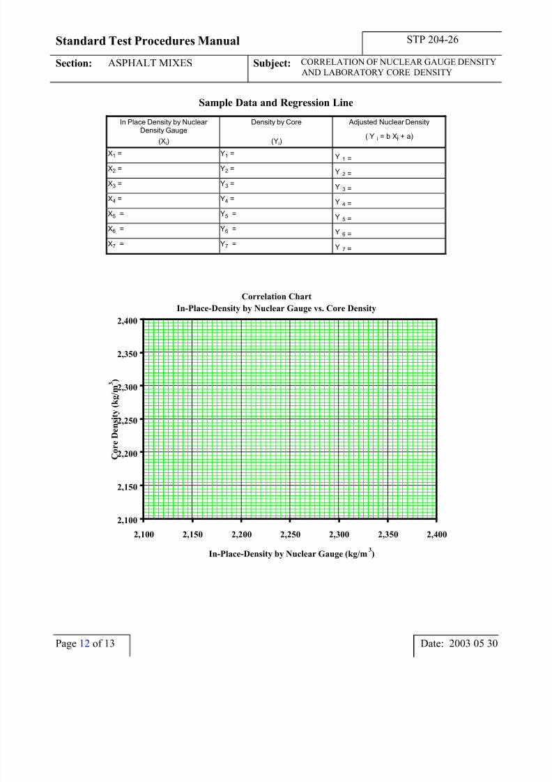
Sample Data and Regression Line

In Place Density by Nuclear Density Gauge

(Xi)

Density by Core

(Yi)

Adjusted Nuclear Density

( i = b Xi + a)$

Y

X1 = Y1 = $Y 1 =

X2 = Y2 = $Y 2 =

X3 = Y3 = $Y 3 =

X4 = Y4 = $Y 4 =

X5 = Y5 = $Y 5 =

X6 = Y6 = $Y 6 =

X7 = Y7 = $Y 7 =

Correlation Chart

In-Place-Density by Nuclear Gauge vs. Core Density

2,100

2,150

2,200

2,250

2,300

2,350

2,400

2,100 2,150 2,200 2,250 2,300 2,350 2,400

In-Place-Density by Nuclear Gauge (kg/m3)

C o r e D e n s i t y

( k g / m 3 )

of 13 Date: 2003 05 30






Criteria for Rejection of Outliers

Sample Size

(n) i

d

d d−

σ

Sample Size

(n) i

d

d d−

σ

6 1.730 12 2.040

7 1.800 13 2.070

8 1.860 14 2.100

9 1.910 15 2.125

10 1.960 16 2.150

11 2.000 17 2.175

Student’s t Distribution Table

Student's t Distribution (5 Degrees of Freedom)

STUDENTS t DISTRIBUTION CURVE

Percent of

Area80.0% 82.5% 85.0% 87.5% 90.0% 92.5% 95.0% 96.0% 97.0% 97.5% 98.0% 99.0%

Degrees of

FreedomValues of t

1 3.0777 3.5457 4.1653 5.0273 6.3137 8.4490 12.7062 15.8945 21.2051 25.4519 31.8210 63.6559

2 1.8856 2.0645 2.2819 2.5560 2.9200 3.4428 4.3027 4.8487 5.6428 6.2054 6.9645 9.9250

3 1.6377 1.7692 1.9243 2.1131 2.3534 2.6808 3.1824 3.4819 3.8961 4.1765 4.5407 5.8408

4 1.5332 1.6465 1.7782 1.9357 2.1318 2.3921 2.7765 2.9985 3.2976 3.4954 3.7469 4.6041

5 1.4759 1.5798 1.6994 1.8409 2.0150 2.2423 2.5706 2.7565 3.0029 3.1634 3.3649 4.0321

6 1.4398 1.5379 1.6502 1.7822 1.9432 2.1510 2.4469 2.6122 2.8289 2.9687 3.1427 3.7074

7 1.4149 1.5092 1.6166 1.7422 1.8946 2.0897 2.3646 2.5168 2.7146 2.8412 2.9979 3.4995

8 1.3968 1.4883 1.5922 1.7133 1.8595 2.0458 2.3060 2.4490 2.6338 2.7515 2.8965 3.3554

9 1.3830 1.4724 1.5737 1.6915 1.8331 2.0127 2.2622 2.3984 2.5738 2.6850 2.8214 3.2498

10 1.3722 1.4599 1.5592 1.6744 1.8125 1.9870 2.2281 2.3593 2.5275 2.6338 2.7638 3.1693

11 1.3634 1.4499 1.5476 1.6606 1.7959 1.9663 2.2010 2.3281 2.4907 2.5931 2.7181 3.1058

12 1.3562 1.4416 1.5380 1.6493 1.7823 1.9494 2.1788 2.3027 2.4607 2.5600 2.6810 3.0545

13 1.3502 1.4347 1.5299 1.6398 1.7709 1.9354 2.1604 2.2816 2.4358 2.5326 2.6503 3.0123

14 1.3450 1.4288 1.5231 1.6318 1.7613 1.9235 2.1448 2.2638 2.4149 2.5096 2.6245 2.9768

15 1.3406 1.4237 1.5172 1.6249 1.7531 1.9132 2.1315 2.2485 2.3970 2.4899 2.6025 2.9467

16 1.3368 1.4193 1.5121 1.6189 1.7459 1.9044 2.1199 2.2354 2.3815 2.4729 2.5835 2.9208

17 1.3334 1.4154 1.5077 1.6137 1.7396 1.8966 2.1098 2.2238 2.3681 2.4581 2.5669 2.8982

18 1.3304 1.4120 1.5037 1.6091 1.7341 1.8898 2.1009 2.2137 2.3562 2.4450 2.5524 2.8784

19 1.3277 1.4090 1.5002 1.6049 1.7291 1.8837 2.0930 2.2047 2.3457 2.4334 2.5395 2.8609

20 1.3253 1.4062 1.4970 1.6012 1.7247 1.8783 2.0860 2.1967 2.3362 2.4231 2.5280 2.8453

21 1.3232 1.4038 1.4942 1.5979 1.7207 1.8734 2.0796 2.1894 2.3278 2.4138 2.5176 2.8314

22 1.3212 1.4016 1.4916 1.5949 1.7171 1.8690 2.0739 2.1829 2.3202 2.4055 2.5083 2.8188

23 1.3195 1.3995 1.4893 1.5922 1.7139 1.8649 2.0687 2.1770 2.3132 2.3979 2.4999 2.8073

24 1.3178 1.3977 1.4871 1.5897 1.7109 1.8613 2.0639 2.1715 2.3069 2.3910 2.4922 2.7970

25 1.3163 1.3960 1.4852 1.5874 1.7081 1.8579 2.0595 2.1666 2.3011 2.3846 2.4851 2.7874

Preview of Student's T(5.00)

0.0

0.2

0.4

0.0 1.2 2.4 3.5 4.7 5.9-1.2-2.4-3.5-4.7-5.9

Date: 2003 05 30 of 13

correlation of nuclear gauge density and laboratory core density procedures

Documents