correlation between cbr values and index properties...

Vol-6 Issue-3 2020 IJARIIE-ISSN(O)-2395-4396

12126 www.ijariie.com 1167

CORRELATION BETWEEN CBR VALUES

AND INDEX PROPERTIES OF SUBGRADE

SOILS: IN THE CASE OF BODITI TOWN

Saol Toyebo Torgano1, Mohammed Sujayath Ali2, Esubalew Tariku Yenealem3, Adane Tadesse Tumato4

1Lecturer, Department of construction Technology and Management, Wolaita Sodo university, SNNPR,

Ethiopia 2 Assistant Professor, Department of construction Technology and Management, Wolaita Sodo university,

SNNPR, Ethiopia 3Lecturer, Department of civil engineering, Wolaita Sodo university, SNNPR, Ethiopia 4Lecturer, Department of Civil engineering, Wolaita Sodo university, SNNPR, Ethiopia

ABSTRACT

The suitability and stability of soil is usually evaluated before its use in construction of pavement. Proper analysis is

necessary to ensure that Civil engineering infrastructures such as roads, buildings, rails, dams, etc. remain safe and

free to withstand settlement and collapse. This paper presents the results of the correlation between California

Bearing Ratio (CBR) and index properties of sub-grade soils in the Boditi town. CBR (California Bearing Ratio) test

is performed to evaluate stiffness modulus and shear strength of subgrade soils. However, CBR test is laborious and

time consuming, particularly when soil is highly plastic. In order to solve this limitation, it may be appropriate to

correlate CBR value of soil with its index properties like grain size analysis, Atterberg limits, and compaction

characteristics such as MDD (Maximum Dry Density) and OMC (Optimum Moisture Content). SLRA (Single Linear

Regression Analysis) and MLRA (Multiple Linear Regression) based Models were utilized. It is seen that MLRA

gave better correlations up to R2 of about 0.984. It is observed that the Soaked CBR value can be predicted with

confidence from LL (Liquid Limit), PI (Plasticity Index) and percent finer while un-soaked CBR value can be

obtained from LL, plasticity index and MDD. Laboratory tests were carried out to determine soaked CBR, LL, PL,

PI, MDD and OMC on soil samples collected from different parts of town. A correlation relationship between CBR

and soil index properties were developed using non-linear and multiple linear regression analysis. Standard

Minitab 16 and Microsoft Excel 2019 software package were used for the analysis.

Keywords: Index Properties, Single Linear Regression Analysis, Multiple Linear Regression Analysis, Predicted

California Bearing Ratio, Regression Analysis and Correlation Analysis, Coefficient of Determination.

1. 1. INTRODUCTION

The suitability and stability of soil is usually evaluated before its use in construction of pavement. Proper analysis is

necessary to ensure that Civil engineering infrastructures such as roads, buildings, rails, dams, etc. remain safe and

free to withstand settlement and collapse. Geographical variability in soil conditions from one location to another

makes it difficult to predict the behavior of soil. As a result, soil conditions at every site must be thoroughly

investigated for proper design [1]. A subgrade soil on which the whole structure of the flexible pavement consists of

a number of layers including pavement rests and for this, CBR is one of the most widely sub-bases, base course,

surfacing etc. which ultimately used methods. This method is mainly used to determine lies on subgrade. Basically,

subgrade is not the physical the stiffness modulus and shear strength of the subgrade part of the pavement but it is

considered as the functional soil and helps in designing the thickness of each layer of pavement [3-4]. If the

subgrade has higher CBR value, this means that it has more strength and will be able to bear more traffic load

coming over it and ultimately the thickness of pavement layers will be small and vice versa [5].

The soaked CBR value of the subgrade soil is of great importance, which is required to be determined as it helps in

assessing the swelling potential and almost the actual strength of subgrade soil over the entire road length. Though

this conventional method helps in evaluating the strength of the subgrade soil by obtaining its soaked CBR value,



but it is quite time consuming and laborious method and also its reproducibility is low [2]. Moreover, this test is

costly as it involves a high-level technical supervision and quality control assessment. Therefore, more samples are

required to be tested in order to achieve better accuracy and to obtain proper idea about the soaked CBR value of

subgrade materials over the entire length of the road which is quite difficult because it is difficult to take large

number of samples. This would result in serious delay in the progress of the project, since in most situations the

materials for earthwork construction come from highly variable sources. Any delay in construction inevitably leads

to rise of project cost [1,4-6].

In Ethiopia, most of the road networks consist of flexible pavement which is made up of different layers such as

sub-grade, sub - base, base course and surface layer. The design and performance of this pavement mainly depend

on the strength of sub-grade material. Sub-grade is the bottom-most layer that serves as the foundation of a road

pavement and the wheel load from the pavement surface is ultimately transferred to the sub-grade [7]. The

California Bearing Ratio (CBR) test is an empirical method of design of flexible pavement. The bearing capacity

of the soil beneath highways, airfield runways and other pavement systems are of great importance to the integrity

of the pavement. This bearing capacity changes from time to time and can vary from place to place within a given

area. The thickness of subgrade depends on CBR value, subgrade that has lower CBR value will have thicker

pavement compared with the sub grade that has higher CBR value and vice versa.

1.2 Objective of the Study

1.2.1 General Objective

The main objective of this thesis is to find correlation between California Bearing Ratio with soil index properties of

subgrade soils recovered from different parts of town.

1.2.2 Specific Objectives

❖ To check and come up with a correlation between CBR values and soil index properties of subgrade soils.

❖ To validate and evaluate the developed correlation using a control test results.

2.LITERATURE REVIEW

2.1 California Bearing Ratio (CBR)

The California Bearing Ratio (CBR), defined as the ratio of the resistance to penetration of a material to the

penetration resistance of a standard crushed stone base material. California Bearing Ratio is the main design input in

pavement construction to assess the stiffness modulus and shear strength of subgrade material. The method was

developed by the California Division of Highways as part of their study in pavement failure at World War II. With

an intention to adopt a more simplified test method to measure the stiffness modulus and shear strength of subgrade

soil a simple test that can be used as an index test was devised. This is where CBR test comes into frame in

measurement of subgrade strength. The CBR test is a simple strength test that compares the bearing capacity of a

material with that of a well graded standard crushed stone base kept in California Division of Highways Laboratory

[8]. This means that the standard crushed stone material should have a CBR value of 100%. The resistance of the

crushed stone under standardized conditions is well established. Therefore, the purpose of a CBR test is to determine

the relative resistance of the subgrade material under the same conditions. The test is an index test; thus, it is not a

direct measure of stiffness modulus or shear strength. The CBR test is essentially a measure of the shearing

resistance of a soil at a known moisture and density conditions. The method of evaluating CBR is standardized in

AASHTO T 193 and ASTM D 1883.

The design of pavement thickness in road construction requires the strength of subgrade soil, sub-base and base-

course material to be expressed in terms of California Bearing Ratio, so that a stable and economic design achieved.

A road section for which a pavement design is undertaken should be sub-divided into subgrade areas where the

subgrade CBR can be reasonably expected to be delineated uniform, i.e. without significant variations, in order to

utilize it in the design of pavement thickness. On the other way, the value of CBR is an indicator of the suitability of

natural subgrade soil as a construction material. If the CBR value of subgrade is high, it means that the subgrade is

strong and as a result, the design of pavement thickness can be reduced in conjunction with the stronger subgrade.

Conversely, if the subgrade soil has low CBR value it indicates that the thickness of pavement shall be increased in

order to spread the traffic load over a greater area of the weak subgrade or alternatively, the subgrade soil shall be

subjected to treatment or stabilization [9].



3.METHODOLOGY 3.1Single Linear Regression Analysis

A SLRA provides an attempt to develop a correlation between two variables only in which one is the response

(dependent) variable and other is the explanatory (independent) variable. In this research work, CBR is the

dependent variable and each individual index properties of soil are independent variable. Graph is plotted between

CBR and index properties of soils and a suitable trend line is drawn through the plotted points for obtaining the

value of coefficient of determination (R2). The value of R2 provides a measure of how well the future outcomes are

likely to be predicted by the model [10]. Generally speaking, any correlation greater than 0.88 is usually considered

as a best fit.

3.2Multiple Linear Regression Analysis

A MLRA provides an attempt to develop a correlation between more than two variables. One is the response

(dependent variable) and others are explanatory (independent) variables. In this research work, CBR is the

dependent variable and all other IP are independent variables. In the equation, CBR value is the function of all other

index properties. Mathematically:

CBR = f (%F, LL, PI, OMC, MDD) ……………………………. (1)

The equation will be created as follows:

Y = bo + b1x1 + b2x2 + b3x3 + b4x4 + ……. Bnxn……….………… (2)

Where bo, b1, b2, b3, b4, bn are constants, Y is CBR and, x1, x2, x3, x4, xn are soil properties considered for analysis.

The values of these constants can be obtained by using Data Analysis Tool bar of Microsoft Excel and then putting

these values with their corresponding soil properties in order to obtain a suitable equation [10].

4. LABORATORY TEST

The samples for this research work have been collected from different section of town. Seven (7) samples have been

collected from depths of about 2-3 feet and laboratory tests for LL, PL, PI, particle size distribution, OMC, MDD

and CBR values (both soaked and unsoaked) have been performed on these samples at Geotechnical Laboratory,

according to AASHTO and ASTM specifications [11-14]. The soil classifications of these samples have been done

according to AASHTO method. The results are given in Table 1 along with % finer passing from #200 sieve (%F)

for each sample.

5.RESULTS AND DISCUSSION

Table 1 summarizes the results of different soil properties from the experiments conducted in the laboratory for

seven samples collected from different locations. Sample Nos. 3 and 4 were classified as A-4 soils and such soils

have very less presence in Jamshoro. Therefore, these samples are not considered for developing correlations. The

range of other soil properties studied in this research work are: PL = 16.49-29.14%, PI = 20.31-29.26% [5]. The

graphs representing laboratory test results for above samples are presented below. Fig. 1 presents the PSD of the soil

samples tested. It is observed that the range of % finer considered for developing correlations by neglecting curves

of sample 3 and 4 because of their irregular behavior comes out to be 58.709-84.794%. Further, the diameters of

particles corresponding to 10% (D10), 30% (D30) and 60% (D60) passing are plotted for all samples through which

Cu (Coefficient of Uniformity) and Cc (Coefficient of Curvature) is determined which helps in determining whether

the soil is well graded or poorly graded. Table 2 presents the D10, D30, D60, together with the Cu and Cc. The Cu is

the ratio of D60 by D10 given by Equation (3):

Cu = D60/D10…………………………………………… (3)

Whereas, the Cu is the ratio of square of D30 by product of D60 and D10 and is given by Equation (4):

Cc = (D30)2/ (D60*D10) …………………………………. (4)

If Cu is greater than 4-6 and Cc lies between 1 and 3, the soil is well graded otherwise it is poorly graded.



Fig. 1. Particle size distribution curves for all soil samples

Sample

No

%F Cu Cc LL

(%)

PL

(%)

PI

(%)

Compaction

Characteristics

CBR values AASH

TO

Classifi

cation OMC

(%)

MDD(g/cc) Unsoaked

(%)

Soak

ed

(%)

1

84.15 133.3 9.48 63 31.2 32 24.5

1.32

33.5 8.42 A-7-5

(poorly

graded

2 87.5 125.0 11.2 71 30.7 40 27.8 1.17 41.3 17.89 A-7-5

(poorly

graded

3

91.06 3.79 0.38 77 34.8 42.

2

24.8 1.37 64.17 33.74 A-7-5

(poorly

graded

4 88.25 4.0 0.35 87 42.2 45 27.4 1.18 11.95 4.558 A-7-5

(poorly

graded

5

92.9 88.89 50.00 86 41.9 44 24.2 1.33 22.06 13.30 A-7-5

(poorly

graded

6 85.15 108.3 77.56 69 29.4 39.

6

28.7 1.20 15.6 10.02 A-7-5

(poorly

graded

7

90.25 22.86 12.87 65 31 34 24.5 1.31 45.19 19.80 A-7-5

(poorly

graded

TABLE 1 LABORATORY TEST RESULTS FOR SOIL SAMPLES

Fig. 2 shows LL curves showing LL corresponding to 20 mm penetration for all the soil samples tested in the

laboratory. Curve of Sample-7 gives the highest liquid limit of about 58.40% and curve of Sample-3 gives the least

liquid limit value of 21.70%. As Samples 3 and 4 were neglected in developing correlations, the least LL is

considered to be 36.80% corresponding to Sample-5. Thus, the range of LL considered for developing correlations is



36.80-58.40%. Fig. 3 shows compaction curves with their peak points representing OMC and MDD of all the soil

samples. Neglecting the results of Samples 3 and 4, the lowest MDD comes out to be 1.740 gm/cm3 for Sample-7

and highest MDD is 2.025 gm/cm3 for Sample-5. Thus, the range considered is 1.740-2.025 gm/cm3. Similarly, the

lowest OMC observed from the graph is 10.50% for Sample5 and the highest is 15.50% for Sample-7. Thus, the

range of OMC considered is 10.50-15.50%. Fig. 4 shows load penetration curves, which help in determining the

Unsoaked CBR values at 2.5and 5mm penetration respectively for all soil samples. The highest of both penetrations

is considered as the CBR value of that particular sample. From Fig. 4, it has been observed that the range of

Unsoaked CBR value considered for developing correlations is 15.571-45.185%.

Fig. 5 shows load penetration curves, which help in determining the Soaked CBR values at 2.5 and 5mm penetration

respectively for all soil samples. From the graph, it has been observed that the range of Soaked CBR value

considered for developing correlations is 8.418-19.805%.

Fig. 2. Liquid limit curves for all soil samples

Fig. 3. Compaction curves for all soil samples

Sample No. D10 D30 D60 Cu Cc Soil Type

1 0.00045 0.016 0.06 133.33 9.48

Poorly Graded

2 0.00048 0.018 0.06 125.0 11.25

3 0.058 0.07 0.22 3.79 0.38

4 0.055 0.065 0.22 4.0 0.35

5 0.0008 0.06 0.074 92.50 60.81

6 0.0006 0.055 0.065 108.33 77.56

7 0.0035 0.06 0.08 22.86 12.86



5.1CORRELATIONS/MODELS

The table of laboratory test results along with the graphs is presented in section 3. Now, correlations/models are

developed in the form of linear equations between CBR values and various index properties first by SLRA and then

collectively by MLRA.

5.1.1Correlations By Single Linear Regression Analysis

The correlations by SLRA were developed and are described in Model 1- 11 (Fig. 6-16) indicating linear

relationship between the variables. Some models gave very low values of reliability R2. However, in this paper, all

models are shown:

Fig. 4. Load-penetration curves for determining unsoaked CBR for all samples

Fig. 5. Load-penetration curves for determining soaked CBR of all soil samples

Model-1: Correlation of Unsoaked California Bearing Ratio (CBRU) With Liquid Limit:

Fig. 6 represents a graph, which shows a correlation between unsoaked CBR and LL for all soil samples. The

mathematical relation between the two parameters is shown in Equation (5). It can be seen that the reliability factor

R2 obtained from this equation is only 0.0413.

CBRU=0.2896(LL) + 17.274 R2 = 0.0413 …………………………. (5)



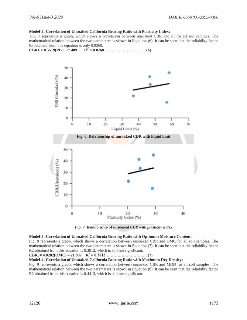
Model-2: Correlation of Unsoaked California Bearing Ratio with Plasticity Index:

Fig. 7 represents a graph, which shows a correlation between unsoaked CBR and PI for all soil samples. The



CBRU= 0.5519(PI) + 17.489 R2 = 0.0268…………………………. (6)

Fig. 6. Relationship of unsoaked CBR with liquid limit

Fig. 7. Relationship of unsoaked CBR with plasticity index

Model-3: Correlation of Unsoaked California Bearing Ratio with Optimum Moisture Content:

Fig. 8 represents a graph, which shows a correlation between unsoaked CBR and OMC for all soil samples. The


R2 obtained from this equation is 0.3812, which is still not significant.

CBRU= 4.0282(OMC) – 21.807 R2 = 0.3812…………………………. (7)

Model-4: Correlation of Unsoaked California Bearing Ratio with Maximum Dry Density:

Fig. 9 represents a graph, which shows a correlation between unsoaked CBR and MDD for all soil samples. The


R2 obtained from this equation is 0.4413, which is still not significant.



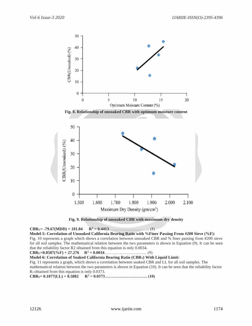
Fig. 8. Relationship of unsoaked CBR with optimum moisture content

Fig. 9. Relationship of unsoaked CBR with maximum dry density

CBRU= -79.67(MDD) + 181.84 R2 = 0.4413………………………... (8)

Model-5: Correlation of Unsoaked California Bearing Ratio with %Finer Passing From #200 Sieve (%F):

Fig. 10 represents a graph which shows a correlation between unsoaked CBR and % finer passing from #200 sieve

for all soil samples. The mathematical relation between the two parameters is shown in Equation (9). It can be seen

that the reliability factor R2 obtained from this equation is only 0.0034.

CBRU=0.0587(%F) + 27.276 R2 = 0.0034……………….………… (9)

Model-6: Correlation of Soaked California Bearing Ratio (CBRS) With Liquid Limit:

Fig. 11 represents a graph, which shows a correlation between soaked CBR and LL for all soil samples. The



CBRS= 0.1077(LL) + 8.5882 R2 = 0.0373…………………………. (10)



Fig. 10. Relationship of unsoaked CBR with % finer

Fig. 11. Relationship of soaked CBR with liquid limit

Model-7: Correlation of Soaked California Bearing Ratio with Plasticity Index:

Fig. 12 represents a graph, which shows a correlation between soaked CBR and PI for all soil samples. The


R2 obtained from this equation is 0.0261.

CBRS=0.2131(PI) + 8.4678 R2 = 0.0261………………………... (11)

Model-8: Correlation of Soaked California Bearing Ratio with Optimum Moisture Content:

Fig. 13 represents a graph, which shows a correlation between soaked CBR and OMC for all soil samples. The



CBRS=0.4624(OMC) + 7.7621 R2 = 0.0328………………… (12)

Fig. 12. Relationship of soaked CBR with plasticity index



Fig. 13. Relationship of soaked CBR with optimum moisture content

Model-9: Correlation of Soaked California Bearing Ratio with Maximum Dry Density:

Fig. 14 represents a graph, which shows a correlation between soaked CBR and MDD for all soil samples. The


R2 obtained from this

equation is 0.1136.

CBRS = -15.81(MDD)+ 43.715 R2 = 0.1136……………………… (13)

Model-10: Correlation of Soaked California Bearing Ratio with % Finer Passing From #200 Sieve (%F):

Fig. 15 represents a graph, which shows a correlation between soaked CBR and % finer passing from #200 sieve for

all soil samples. The mathematical relation between the two parameters is shown in Equation (14). It can be seen

that the reliability factor R2 obtained from this equation is 0.1806 which is still not significant.

CBRS=-0.1681(%F) + 26.02 R2 = 0.1806……………………… (14)

Fig. 14. Relationship of soaked CBR with maximum dry density

Fig. 15. Relationship of soaked CBR with % finer



Model-11: Correlation of Soaked California Bearing Ratio (CBRS) With Unsoaked California Bearing Ratio:

Fig. 16 represents a graph, which shows a correlation between soaked CBR and unsoaked CBR for all soil samples

[15]. The mathematical relation between the two parameters is shown in Equation (15). It can be seen that the

reliability factor R2 obtained from this equation is 0.5153 which is still not significant.

CBRS=0.2807(CBRU) + 5.0352 R2 = 0.5153………………………. (15)

A brief summary of the developed SLRA models for both Soaked and Unsoaked CBR are given in Table 3.

Fig. 16. Relationship of soaked CBR with unsoaked CBR

From the above developed SLRA models for unsoaked CBR, based on the values of coefficient of determination

(R2), it has been noted that Model-4 provides a better correlation with MDD with value of R2 = 0.4413. Similarly,

for soaked CBR, Model-10 provides a better correlation with % Finer with value of R2 = 0. 1806.On the other hand,

the correlation between soaked and unsoaked CBR has been found to be a better correlation with a value of R2 =

0.5153.

5.2 Correlations by Multiple Linear Regression Analysis

This analysis has been performed by taking CBR as function of more than one independent variables [Equation (1)].

Now, the equations which have been obtained through MLRA by adopting Microsoft Excel solution are given in

Table 4 along with their model number. From the above developed MLRA models for Soaked CBR, based on the

values of coefficient of determination (R2) and Adjusted Coefficient of Determination (Adj R2), it has been noted

that Model-13 provides a better correlation with LL, PI and % Finer with value of R2 = 0.984 and Adjusted R2 =

0.935. Similarly, for Unsoaked CBR, correlations/models

developed are shown in Table 5. From the above developed MLRA models for Unsoaked CBR, based on the values

of coefficient of determination (R2) and Adjusted Coefficient of Determination (Adj R2), it can be noted that Model-

32 provides a better correlation of Unsoaked CBR with LL, PI and MDD with value of R2= 0.971 and Adjusted R2 =

0.884.

Model No. Correlation/Model R2

1 CBRU= 0.2896(LL) + 17.274 0.0413

2 CBRU= 0.5519(PI) + 17.489 0.0268



3 CBRU= 4.0282(OMC) - 21.807 0.3812

4 CBRU= -79.67(MDD) + 181.84 0.4413

5 CBRU=0.0587(%F) + 27.276 0.0034

6 CBRS= 0.1077(LL) + 8.5882 0.0373

7 CBRS=0.2131(PI) + 8.4678 0.0261

8 CBRS=0.4624(OMC) + 7.7621 0.0328

9 CBRS = -15.81(MDD)+ 43.715 0.1136

10 CBRS=-0.1681(%F) + 26.02 0.1806

11 CBRS=0.2807(CBRU) + 5.0352 0.5153

TABLE 3. DEVELOPED CORRELATIONS FOR UNSOAKED AND SOAKED CBR VALUES (SLRA)

6. VALIDATION ANALYSIS From section 4, it is observed that high reliability for CBR prediction is observed from MLRA instead of SLRA. So

now, equations of MLRA are utilized for obtaining relation between predicted and actual CBR (Table 6). Also, the

graph is plotted to show the difference in values between experimental and predicted CBR for each sample. For

Soaked CBR: CBRS =11.2525(LL)-26.4144(PI)-0.3024(%F) +153.7175(16) R2= 0.984, Adj R2= 0.935 Now, the

graph between predicted and actual CBR (Soaked) along with line of equality is presented in Fig, 17. The trend line

in Fig. 17 shows that the ratio of predicted to actual CBR value is 1 i.e. P/A =1. Points above this line of equality

indicate those samples whose predicted CBR value is higher than their actual CBR value and vice versa. From Fig.

17, it is observed that predicted CBR values of Sample-1, 6 and 7 slightly deviate from the line of equality while the

remaining samples predicted CBR values scatters near the line of equality. The difference between

experimental/actual and predicted CBR values is graphically shown below:

Fig. 18 represents difference in values of predicted and actual CBR value in soaked condition for each soil sample in

a graphical format. It can be seen that predicted CBR values of Samples 2, 5 and 6 under estimate their actual CBR

values, but for Sample 1 and 7, predicted CBR values over estimate their actual CBR values. Fig. 18 depicts the

results of Soaked CBR value obtained from laboratory results as well as model.


1 CBRS = 7.9602(LL)-18.5855(PI)+94.8082 0.478

2 CBRS = 0.0729(LL)+0.2140(OMC)+7.4679 0.040

3 CBRS = 60.1486-0.0954(LL)-22.0345(MDD) 0.125

4 CBRS = 0.0992(LL)-0.1655(%F) +20.9566 0.212

5 CBRS = 0.0824(PI)+0.3456(OMC)+7.2138 0.035

6 CBRS =66.5421-0.2981(PI)-23.8927(MDD) 0.135

7 CBRS = 0.1836(PI)-0.1651(%F) +21.1395 0.200

8 CBRS= 537.9573-10.4525(OMC)-204.4219(MDD) 0.726

9 CBRS = 0.6217(OMC)-0.1812(%F) +18.7382 0.239

10 CBRS = 54.7316-15.3367(MDD)-0.1650(%F) 0.287



11 CBRS=9.1437(LL)-21.0468(PI)-0.8825(OMC)+110.8469 0.524

12 CBRS = 7.9210(LL)-18.5035(PI)-0.4965(MDD)+95.5896 0.478

13 CBRS =11.2525(LL)-26.4144(PI)-0.3024(%F) +153.7175 0.984

14 CBRS = 589.7867-0.1925(LL)-10.8470(OMC)-224.1055(MDD) 0.773

15 CBRS = 18.8030-0.0064(LL)+0.6442(OMC)-0.1819(%F) 0.239

16 CBRS = 73.0295-0.1057(LL)-22.2298(MDD)-0.1663(%F) 0.302

17 CBRS = 596.3103-0.5054(PI)-10.8681(OMC)-225.6242(MDD) 0.787

18 CBRS =19.9079-0.1233(PI)+0.8015(OMC)-0.1870(%F) 0.243

19 CBRS =81.3928-0.3450(PI)-24.6802(MDD)-0.1686(%F) 0.316

20 CBR(Soaked) = 938.5039-19.3692(OMC)-366.2257(MDD)+0.3156(%F) 0.917

TABLE 4. DEVELOPED CORRELATIONS FOR SOAKED CBR VALUE (MLRA)


21 CBRU = 293.4964+25.4466(LL)-59.5422(PI) 0.734

22 CBRU = 6.8302(OMC)-0.8217(LL)-18.4886 0.529

23 CBRU = 374.0235-1.1153(LL)-152.4578(MDD) 0.685

24 CBRU = 0.2930(LL)+0.0663(%F) +12.3209 0.046

25 CBRU = 6.9941(OMC)-2.0923(PI)-7.8884 0.560

26 CBRU = 392.0103-2.7448(PI)-154.0842(MDD) 0.720

27 CBRU = 0.5640(PI)+0.0678(%F) +12.2863 0.031

28 CBRU = 474.0850-6.1806(OMC)-191.1960(MDD) 0.474

29 CBRU = 4.0517(OMC)-0.0268(%F)-20.1844 0.382

30 CBRU = 0.0751(%F)-79.8853(MDD)+176.8267 0.447

31 CBRU = 19.5963(LL)-47.3755(PI)+4.3622(OMC)+214.2133 0.904

32 CBRU = 17.3174(LL)-42.5467(PI)-102.9336(MDD)+455.5159 0.971

33 CBRU = 28.4911(LL)-66.7818(PI)-0.2796(%F) +347.9718 0.800

34 CBRU = 795.1081-1.1925(LL)-8.6238(OMC)-313.1128(MDD) 0.748

35 CBRU = 7.0988(OMC)-0.8712(LL)-0.1136(%F)-11.4105 0.541

36 CBRU = 369.2812-1.1115(LL)-152.3859(MDD)-0.0612(%F) 0.689

37 CBRU = 809.8604-2.9083(PI)-8.5721(OMC)-313.1981(MDD) 0.782

38 CBRU = 1.0451-2.2370(PI)+7.3149(OMC)-0.1316(%F) 0.576

39 CBRU = 387.9331-2.7319(PI)-153.8680(MDD)+0.0463(%F) 0.722

40 CBRU = 1443.6615-27.7645(OMC)-582.8637(MDD)+0.7639(%F) 0.645

TABLE 5. DEVELOPED CORRELATIONS FOR UNSOAKED CBR VALUE (MLRA)



Sample No. Actual CBR Value (%) Predictive CBR Value (%) Difference in

Values

1 8.418 9.262 -0.844

2 17.892 17.396 0.496

5 13.302 13.161 0.141

6 10.002 9.363 0.639

7 19.805 20.225 -0.420

` TABLE 6. VALIDATION OF DEVELOPED CORRELATION FOR SOAKED CBR`

For Unsoaked CBR,

CBRU = 17.3174(LL)-42.5467(PI)-102.9336(MDD)+455.5159…………………. (17)

R2= 0.971, Adj R2 = 0.884

Now, the graph between predicted and actual CBR (Unsoaked) along with line of equality is presented in Fig. 19. It

is observed that predicted CBR values of Sample 1, 5 and 7 slightly deviate from the line of equality while the

remaining samples predicted CBR values scatters near the line of equality. Moreover, the predicted CBR values of

Sample 1, 2 and 6 are higher than their actual CBR values while the predicted CBR values of Sample 5 and 7are

lower than their actual CBR values (Table 7).

The difference between experimental/actual and predicted CBR values is shown graphically below:

Fig. 20 represents difference in values of predicted and actual CBR value in unsoaked condition for each soil sample

in a graphical format. It can be clearly seen that predicted CBR values of Sample 5 and 7 under estimate their actual

CBR values, but for Sample 1, 2 and 6, predicted CBR values over estimate their actual CBR values.

Fig. 17. Graph of predicted vs actual CBR in soaked condition



Fig. 18. Graph of CBR value vs sample number in soaked condition

Fig. 19. Graph of predicted vs actual CBR in unsoaked condition

Fig. 20. Graph of CBR value vs sample number in unsoaked condition

Sample No. Actual CBR Value (%) Predictive CBR Value (%) Difference in Values

1 33.465 36.379 -2.914

2 41.310 41.745 -0.435



5 22.059 20.232 1.827

6 15.571 16.405 -0.834

7 45.185 42.831 2.354

TABLE 7. VALIDATION OF DEVELOPED CORRELATION FOR UNSOAKED CBR Difference in Values

6. CONCLUSION From the results of the research, the following conclusions can be drawn:

(i) Based on the above laboratory tests, no any reliable SLRA relationship exists for predicting Soaked as well as

Un-Soaked CBR value from index properties.

(ii) The highest coefficient of determination obtained for Soaked CBR is 0.1806 while correlating Soaked CBR with

% finer, and the highest coefficient of determination obtained for Un-Soaked CBR is 0.4413 while correlating Un-

Soaked CBR with MDD.

(iii) Un-Soaked CBR value provides a relationship with MDD through SLRA with coefficient of determination R2=

0.4413, which is not suitable.

(iv) The correlation of Soaked CBR with LL, PI and %Finer by utilizing MLRA approach gives a good relationship

with R2 = 0.984 which is CBR (Soaked) = 11.2525(LL) - 26.4144(PI) - 0.3024(%F) + 153.7175 The correlation of

Un-Soaked CBR with LL, PI and MDD by utilizing MLRA approach gives a good relationship with R2 = 0.971,

CBR (Un-Soaked) = 17.3174(LL) - 42.5467(PI) - 102.9336(MDD) + 455.5159

(vi) It is observed that CBR values decreases with increase in PI and increases with increase in LL.

(vii) From the developed correlation, it can be seen that the Soaked CBR value is largely dependent on LL and PI of

soil whereas, the effect of % Finer is minor.

(viii) For Unsoaked CBR, the values are largely dependent on LL, PI and MDD.

7. REFERENCES [1] Charman, J H. (1988). Laterite in road pavements. Construction Industry Research and Information Association,

London.

[2]Ramasubbarao, G.V., and Siva, S.G., “Predicting Soaked CBR Value of Fine-Grained Soils using Index and

Compaction Characteristics”, Jordan Journal of Civil Engineering, Volume 7, No. 3, pp. 354-360, Jordan, 2013.

[3] Patel, R.S., and Desai, M.D., “CBR Predicted by Index Properties for Alluvial Soils of South Gujarat”,

Proceedings of Indian Geotechnical Conference, pp. 79-82, India, December 16-18, 2010.

[4] Janjua, Z.S., and Chand, J., “Correlation of CBR with Index Properties of Soil”, International Journal of Civil

Engineering and Technology, Volume 7, No. 5, pp. 57-62, India, 2016.

[5] Shirur, N.B., and Hiremath, S.G., “Establishing Relationship between CBR Value and Physical Properties of

Soil”, IOSR Journal of Mechanical and Civil Engineering, Volume 11, No. 5, pp. 26-30, India, 2014

[6] Patel, M.A., and Patel, H.S., “Correlation between Physical Properties and California Bearing Ratio Test on

Soils of Gujarat Region in Both Soak and Un-Soak Condition”, International Journal of Civil Engineering and

Technology, Volume 3, No. 2, pp. 50-59, India, 2012.

[7] Rakaraddi, P. G., and Gomarsi, V. (2015). Establishing Relationship between CBR with different Soil Properties.

International Journal of Research in Engineering and Technology, 4 (2): 182 - 188.

[8] Yang, H., Pavement Design and Analysis, Pearson Education Inc., New Saddle River, NJ, 2004.

[9] Ethiopian Road Authority, Pavement Design Manual Volume 1, chapter 3 Subgrade, Brehanena Selam Printing

Enterprise, Addis Ababa, 2002.

[10] Rakaraddi, P.G., and Gomarsi, V., “Establishing Relationship between CBR with Different Soil Properties”,

International Journal of Research in Engineering and Technology, Volume 4, No. 2, pp. 182-188, India, 2015.

[11]Das, B.M., “Principles of Geotechnical Engineering”, 7th Edition CL Engineering Publisher, USA, 2009.

[12]Punmia, B.C., Kumar, A., and Jain, A.K., “Soil Mechanics & Foundation Engineering”, 16th Edition, Laxmi

Publisher, India, 2015,

[13] Garg, S.K., “Soil Mechanics & Foundation Engineering”, 4th Revised Edition, Khanna Publisher, India, 2001.

[14] ASTM D1883-07, “Standard Test Method for CBR (California Bearing Ratio) of Laboratory-Compacted

Soils”, American Society for Testing and Materials, USA, 2007.

correlation between cbr values and index properties...

Documents