correcting writing errors with convolutional neural networks

Correcting Writing Errors with Convolutional Neural Networks

by

Nicholas A. Dronen

B.A., Moorhead State University, 1993

M.S., University of Colorado, 2006

A thesis submitted to the

Faculty of the Graduate School of the

University of Colorado in partial fulfillment

of the requirements for the degree of

Doctor of Philosophy

Department of Computer Science

2016

This thesis entitled:Correcting Writing Errors with Convolutional Neural Networks

written by Nicholas A. Dronenhas been approved for the Department of Computer Science

Prof. James H. Martin

Prof. Peter W. Foltz

Date

The final copy of this thesis has been examined by the signatories, and we find that both the content and theform meet acceptable presentation standards of scholarly work in the above mentioned discipline.

iii

Dronen, Nicholas A. (Ph.D., Computer Science)

Correcting Writing Errors with Convolutional Neural Networks

Thesis directed by Prof. James H. Martin

Convolutional neural networks (ConvNets) have been shown to be effective at a variety of natural

language processing tasks. To date, their utility for correcting errors in writing has not been investigated.

Writing error correction is important for a variety of computer-based methods for the assessment of writing.

In this thesis, we apply ConvNets to a number of tasks pertaining to writing errors – including non-word error

detection, isolated non-word correction, context-dependent non-word correction, and context-dependent real

word correction – and find them to be competitive with or superior to a number of existing approaches.

On these tasks, ConvNets function as discriminative language models, so on several tasks we compare

ConvNets to probabilistic language models. Non-word error detection, for instance, is usually performed

with a dictionary that provides a hard, Boolean answer to a word query. We evaluate ConvNets as a soft

dictionary that provides soft, probabilistic answers to word queries. Our results indicate that ConvNets

perform better in this setting than traditional probabilistic language models trained with the same examples.

Similarly, in context-dependent non-word error correction, high-performing systems often make use of a

probabilistic language model. We evaluate ConvNets and other neural architectures on this task and find

that all neural network models outperform probabilistic language models, even though the networks were

trained with two orders of magnitude fewer examples.

Dedication

To Cheng-Hsi and Coraline, for their patience and forbearance during the many years I spent prepar-

ing to do this work. Now I can be a husband and father again.

v

Acknowledgements

Many thanks to my advisors James H. Martin and Peter W. Foltz for their encouragement and support

while I did this work, to my colleagues Mark Rosenstein and Lakshmi Ramachandran for their thoughtful

comments, and to Pearson, my employer, for financial support. The non-word generative model we intro-

duce is the result of a collaboration with Scott Hellman, another Pearson colleague. Thanks also to Chris

Rank for his careful editing of the manuscript.

Contents

Chapter

1 Introduction 1

1.1 Motivation . . . . . . . . . . . . . . . . . . . . . . . . . . . . . . . . . . . . . . . . . . . . 1

1.2 Problems and Contributions . . . . . . . . . . . . . . . . . . . . . . . . . . . . . . . . . . 4

1.2.1 Non-word Error Detection . . . . . . . . . . . . . . . . . . . . . . . . . . . . . . . 4

1.2.2 Isolated Non-word Error Correction . . . . . . . . . . . . . . . . . . . . . . . . . . 6

1.2.3 Contextual Non-word Error Correction . . . . . . . . . . . . . . . . . . . . . . . . 7

1.2.4 Real-word Error Correction . . . . . . . . . . . . . . . . . . . . . . . . . . . . . . 7

1.2.5 Generative Spelling Error Model . . . . . . . . . . . . . . . . . . . . . . . . . . . . 8

1.3 Report Summary and Organization . . . . . . . . . . . . . . . . . . . . . . . . . . . . . . . 8

1.4 Notation and Terminology . . . . . . . . . . . . . . . . . . . . . . . . . . . . . . . . . . . 10

1.4.1 Notation . . . . . . . . . . . . . . . . . . . . . . . . . . . . . . . . . . . . . . . . 10

1.4.2 Terminology . . . . . . . . . . . . . . . . . . . . . . . . . . . . . . . . . . . . . . 10

1.5 Research Questions . . . . . . . . . . . . . . . . . . . . . . . . . . . . . . . . . . . . . . . 12

1.5.1 Research Question 1 . . . . . . . . . . . . . . . . . . . . . . . . . . . . . . . . . . 12




vii

2 Literature Review 17

2.1 Spelling Error Detection and Correction . . . . . . . . . . . . . . . . . . . . . . . . . . . . 17

2.1.1 Non-word Error Detection . . . . . . . . . . . . . . . . . . . . . . . . . . . . . . . 18

2.1.2 Isolated Non-word Error Correction . . . . . . . . . . . . . . . . . . . . . . . . . . 19

2.1.3 Context-dependent Correction . . . . . . . . . . . . . . . . . . . . . . . . . . . . . 25

2.1.4 Query Correction and Web Corpora . . . . . . . . . . . . . . . . . . . . . . . . . . 28

2.2 Grammatical Error Detection and Correction . . . . . . . . . . . . . . . . . . . . . . . . . . 30

2.3 ConvNet Language Models . . . . . . . . . . . . . . . . . . . . . . . . . . . . . . . . . . . 31

2.4 Additive Noise as a Regularizer . . . . . . . . . . . . . . . . . . . . . . . . . . . . . . . . 32

2.5 Unsupervised Pre-training . . . . . . . . . . . . . . . . . . . . . . . . . . . . . . . . . . . 33

2.6 Unsupervised Training of ConvNets . . . . . . . . . . . . . . . . . . . . . . . . . . . . . . 34

2.7 Supervised ConvNets for Natural Language Processing Tasks . . . . . . . . . . . . . . . . . 34

3 Study 1: The Convolutional Network as a Soft Dictionary 36

3.1 Hyperparameters for Effective Non-word Error Detection . . . . . . . . . . . . . . . . . . . 40

3.2 Error Simulation . . . . . . . . . . . . . . . . . . . . . . . . . . . . . . . . . . . . . . . . 41

3.3 Comparison to Probabilistic Language Models . . . . . . . . . . . . . . . . . . . . . . . . . 48

3.4 Conclusion . . . . . . . . . . . . . . . . . . . . . . . . . . . . . . . . . . . . . . . . . . . 56

4 Study 2: Isolated Non-word Error Correction 57

4.1 Corpora . . . . . . . . . . . . . . . . . . . . . . . . . . . . . . . . . . . . . . . . . . . . . 58

4.2 Baselines . . . . . . . . . . . . . . . . . . . . . . . . . . . . . . . . . . . . . . . . . . . . 61

4.2.1 Near-miss and Aspell RETRIEVE . . . . . . . . . . . . . . . . . . . . . . . . . . 61

4.2.2 Jaro-Winkler RANK . . . . . . . . . . . . . . . . . . . . . . . . . . . . . . . . . . 62

4.2.3 Random Forest RANK . . . . . . . . . . . . . . . . . . . . . . . . . . . . . . . . . 63

4.3 Binary ConvNet Model . . . . . . . . . . . . . . . . . . . . . . . . . . . . . . . . . . . . . 67

4.3.1 Architecture . . . . . . . . . . . . . . . . . . . . . . . . . . . . . . . . . . . . . . . 67

4.3.2 Evaluation . . . . . . . . . . . . . . . . . . . . . . . . . . . . . . . . . . . . . . . 69

viii

4.4 Multiclass ConvNet Model . . . . . . . . . . . . . . . . . . . . . . . . . . . . . . . . . . . 76

4.4.1 Architecture . . . . . . . . . . . . . . . . . . . . . . . . . . . . . . . . . . . . . . . 76

4.4.2 Evaluation . . . . . . . . . . . . . . . . . . . . . . . . . . . . . . . . . . . . . . . 76

4.5 Conclusion . . . . . . . . . . . . . . . . . . . . . . . . . . . . . . . . . . . . . . . . . . . 80

5 Study 3: Contexual Non-word Error Correction 81

5.1 Corpus . . . . . . . . . . . . . . . . . . . . . . . . . . . . . . . . . . . . . . . . . . . . . . 83

5.2 Models . . . . . . . . . . . . . . . . . . . . . . . . . . . . . . . . . . . . . . . . . . . . . 83

5.2.1 Google Web 1T 5-gram Language Model RANK . . . . . . . . . . . . . . . . . . . 83

5.2.2 Context-Dependent ConvNets RANK . . . . . . . . . . . . . . . . . . . . . . . . . 84

5.2.3 Feed-Forward Embedding Network RANK . . . . . . . . . . . . . . . . . . . . . . 85

5.3 Experiments . . . . . . . . . . . . . . . . . . . . . . . . . . . . . . . . . . . . . . . . . . . 85

5.4 Conclusion . . . . . . . . . . . . . . . . . . . . . . . . . . . . . . . . . . . . . . . . . . . 90

6 Study 4: Correcting Preposition Errors with Convolutional Networks and Contrasting Cases 91

6.1 Feature Engineering Versus Learning . . . . . . . . . . . . . . . . . . . . . . . . . . . . . . 92

6.2 ConvNets with Contrasting Cases . . . . . . . . . . . . . . . . . . . . . . . . . . . . . . . 93

6.3 Corpora . . . . . . . . . . . . . . . . . . . . . . . . . . . . . . . . . . . . . . . . . . . . . 94

6.4 Modeling . . . . . . . . . . . . . . . . . . . . . . . . . . . . . . . . . . . . . . . . . . . . 96

6.5 Experiments . . . . . . . . . . . . . . . . . . . . . . . . . . . . . . . . . . . . . . . . . . . 97

6.6 Hyperparameter Selection . . . . . . . . . . . . . . . . . . . . . . . . . . . . . . . . . . . 98

6.7 Wikipedia . . . . . . . . . . . . . . . . . . . . . . . . . . . . . . . . . . . . . . . . . . . . 99

6.8 Encarta . . . . . . . . . . . . . . . . . . . . . . . . . . . . . . . . . . . . . . . . . . . . . 103

6.9 Project Gutenberg . . . . . . . . . . . . . . . . . . . . . . . . . . . . . . . . . . . . . . . . 105

6.10 Human Judgments . . . . . . . . . . . . . . . . . . . . . . . . . . . . . . . . . . . . . . . 105

6.11 Conclusion . . . . . . . . . . . . . . . . . . . . . . . . . . . . . . . . . . . . . . . . . . . 106

7 Conclusion 108

Tables

Table

2.1 Encodings produced by several phonetic matching algorithms. . . . . . . . . . . . . . . . . 22

3.1 Set for first stage of hyperparameter selection . . . . . . . . . . . . . . . . . . . . . . . . . 40

3.2 Confusion matrix of best-performing model found by grid search. . . . . . . . . . . . . . . 41

3.3 Performance metrics of best-performing model found by grid search. . . . . . . . . . . . . . 41

3.4 Confusion matrices of models trained using positive examples from the Aspell English dic-

tionary and artificial negative examples created via different edit operations. . . . . . . . . . 43

3.5 Confusion matrix of model trained using artificial negative examples created via a single

transpose. . . . . . . . . . . . . . . . . . . . . . . . . . . . . . . . . . . . . . . . . . . . . 44


insertion. . . . . . . . . . . . . . . . . . . . . . . . . . . . . . . . . . . . . . . . . . . . . 45


substitution. . . . . . . . . . . . . . . . . . . . . . . . . . . . . . . . . . . . . . . . . . . . 46


deletion. . . . . . . . . . . . . . . . . . . . . . . . . . . . . . . . . . . . . . . . . . . . . . 47

3.9 Confusion matrices of discriminative models used to distinguish non-words and real words. . 49

3.10 Accuracies of ConvNet and language model classifiers at classifying non-English words as

English non-words. . . . . . . . . . . . . . . . . . . . . . . . . . . . . . . . . . . . . . . . 52

3.11 Probability that a word is an English word according to the ConvNet and language model

classifier. The words shown were sampled at random from each language’s vocabulary. . . . 53

x

4.1 Summaries of the corpora of spelling errors and corrections archived by Prof. Mitton. . . . . 58

4.2 Edits learned from misspellings of “America”. . . . . . . . . . . . . . . . . . . . . . . . . . 60

4.3 The ten most-frequent edits from our database of learned edits that can be applied to “brick”.

The probabilities are computed over the ten edits only, for purposes of illustration. . . . . . . 60

4.4 A candidate list retrieved using Metaphone for phonetic matching. . . . . . . . . . . . . . . 63

4.5 Features used to train the random forest RANK model. . . . . . . . . . . . . . . . . . . . . 66

4.6 The number of generated non-words in the corpus used for evaluation, conditioned on the

length of the non-word. The number of non-words of a given length is a function of (1) the

number of real words of that length in the Aspell English dictionary and (2) the number of

learned edits that can be applied to the words of that length. Typically, the longer a word is,

the more opportunities exist to apply a learned edit. . . . . . . . . . . . . . . . . . . . . . . 70

4.7 Accuracy at rank K of two baselines and ConvNet binary model on the four Mitton corpora. 75

4.8 Accuracy at rank K of the Jaro-Winkler and multiclass ConvNet RANK components. . . . 79

5.1 The number of words matching the regular expression at the head of each column. ^.aLETTERe$

means any word that begins with any character, has “a” as its second letter, has LETTER as

its third character, and ends with “e”. . . . . . . . . . . . . . . . . . . . . . . . . . . . . . . 82

5.2 Accuracy at K of Word and Character ConvNet models trained with additive noise from

N (0, σ2) between the convolutional layer and the subsequent non-linearity. . . . . . . . . . 87

5.3 Rank correlations of the rank of a word in the candidate list and it’s unigram probability in

the Google Web 1T 5-gram corpus. All values are significant. . . . . . . . . . . . . . . . . . 89

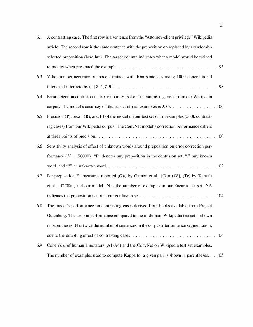
6.2 Width-5 windows of a contrasting case (cf. Table 6.1) and corresponding model inputs,

assuming that the indices of “on” and “for” in the vocabulary are 1 and 4, respectively. The

window size here is only for purposes of illustration; we consider and evaluate multiple

window sizes in Section 6.5, including the entire sentence. . . . . . . . . . . . . . . . . . . 95

xi

6.1 A contrasting case. The first row is a sentence from the “Attorney-client privilege” Wikipedia

article. The second row is the same sentence with the preposition on replaced by a randomly-

selected preposition (here for). The target column indicates what a model would be trained

to predict when presented the example. . . . . . . . . . . . . . . . . . . . . . . . . . . . . . 95

6.3 Validation set accuracy of models trained with 10m sentences using 1000 convolutional

filters and filter widths ∈ { 3, 5, 7, 9 }. . . . . . . . . . . . . . . . . . . . . . . . . . . . . . 98

6.4 Error detection confusion matrix on our test set of 1m contrasting cases from our Wikipedia

corpus. The model’s accuracy on the subset of real examples is .935. . . . . . . . . . . . . . 100

6.5 Precision (P), recall (R), and F1 of the model on our test set of 1m examples (500k contrast-

ing cases) from our Wikipedia corpus. The ConvNet model’s correction performance differs

at three points of precision. . . . . . . . . . . . . . . . . . . . . . . . . . . . . . . . . . . . 100

6.6 Sensitivity analysis of effect of unknown words around preposition on error correction per-

formance (N = 50000). “P” denotes any preposition in the confusion set, “.” any known

word, and “?” an unknown word. . . . . . . . . . . . . . . . . . . . . . . . . . . . . . . . . 102

6.7 Per-preposition F1 measures reported (Ga) by Gamon et al. [Gam+08], (Te) by Tetrault

et al. [TC08a], and our model. N is the number of examples in our Encarta test set. NA

indicates the preposition is not in our confusion set. . . . . . . . . . . . . . . . . . . . . . . 104

6.8 The model’s performance on contrasting cases derived from books available from Project

Gutenberg. The drop in performance compared to the in-domain Wikipedia test set is shown

in parentheses. N is twice the number of sentences in the corpus after sentence segmentation,

due to the doubling effect of contrasting cases . . . . . . . . . . . . . . . . . . . . . . . . . 104

6.9 Cohen’s κ of human annotators (A1-A4) and the ConvNet on Wikipedia test set examples.

The number of examples used to compute Kappa for a given pair is shown in parentheses. . . 105

Figures

Figure

1.1 The steps of a spelling error system in different application scenarios. . . . . . . . . . . . . 3

1.2 When used for non-word error detection, a ConvNet can function either as a binary or a

multiclass classifier. . . . . . . . . . . . . . . . . . . . . . . . . . . . . . . . . . . . . . . . 5

1.3 A component-level view of ConvNets for isolated non-word error correction. . . . . . . . . 7

1.4 Roadmap of this thesis . . . . . . . . . . . . . . . . . . . . . . . . . . . . . . . . . . . . . 9

1.5 A convolutional network . . . . . . . . . . . . . . . . . . . . . . . . . . . . . . . . . . . . 11

1.6 Convolutional network architectures for isolated non-word error correction. . . . . . . . . . 14

1.7 Convolutional network architectures for contextual non-word error correction. . . . . . . . . 15

1.8 A hypothetical multiclass classification ConvNet that functions as a RANK component for

real-word error correction. It takes the context of the possible error as input. The output

of the network is a probability distribution over the words in the confusion set C. In this

case C ∈ quiet quite. The probabilities rank the quality of the possible replacements. The

blacked-out word embedding indicates that the network is not allowed to see the word in the

confusion set at the center of the context; the network is expected to predict the word that

should be at that position. . . . . . . . . . . . . . . . . . . . . . . . . . . . . . . . . . . . . 16

3.1 The density of probabilities that a non-English word from one of four European languages

is English, according to a ConvNet (top) and a language model classifier (bottom). . . . . . 54

3.2 The density of probabilities that a brand name or company is English according to a ConvNet. 55

xiii

4.1 Distributions in the Mitton corpora. The top figure shows the distribution of the lengths

of the non-words. The bulk of the errors appears to be in the range 4-10 characters. The

Holbrook corpus’ distribution is right skew, exhibiting a noticeably higher proportion of

shorter long words than exists in the other corpora. The bottom figure shows the distribution

of edit distances between the non-words and corrections in a corpus. . . . . . . . . . . . . . . 59

4.2 Frequency distributions of the length of the candidate lists returned by Aspell or simple edit

distance retrieval on each corpus. . . . . . . . . . . . . . . . . . . . . . . . . . . . . . . . . 64

4.3 The architecture of our binary ConvNet. . . . . . . . . . . . . . . . . . . . . . . . . . . . . 68

4.4 Accuracy at rank K of binary ConvNet model conditioned on the length of the non-word. . . 72

4.5 The difference of accuracy at rank K of the binary ConvNet model versus Jaro-Winkler,

conditioned on the length of the non-word. The upper line of a ribbon almost always rep-

resents the performance of the ConvNet, except at K = 10 for four-character non-words,

where Jaro-Winkler is slightly more accurate. . . . . . . . . . . . . . . . . . . . . . . . . . 73

4.6 The difference of accuracy at rank K between two models, conditioned on the length of the

non-word. . . . . . . . . . . . . . . . . . . . . . . . . . . . . . . . . . . . . . . . . . . . . 74

4.7 The architecture of our multiclass ConvNet. . . . . . . . . . . . . . . . . . . . . . . . . . . 77

5.1 Accuracy at k of the networks and the Google Web 1T 5-gram corpus baseline. The Word

and Character ConvNet is the one trained with σ2 of 0. . . . . . . . . . . . . . . . . . . . . 86

5.2 Examples of rankings from basline and ConvNet models. The correct candidate is shown in

green. P(Candidate) is the unigram probability of the candidate word in the Google Web 1T

5-gram corpus. For brevity, a subset of the candidate list is shown. . . . . . . . . . . . . . . 88

Chapter 1

Introduction

1.1 Motivation

Detecting and correcting errors in writing is useful in many situations. Collaborative online encyclo-

pedias – because they are written by many authors with variable writing abilities – can benefit from tools that

detect and correct errors. Rapid digital writing (e.g. email, SMS, Twitter, and other short-form platforms)

increases typographic errors, hindering communication. Components for detecting and correcting errors are

also useful in software applications that evaluate learner writing; this thesis is motivated by the need for

high-quality error detection and correction in these applications.

Consider an interactive writing tutor application that helps learners improve their writing skills. When

a learner makes a mistake, the application can detect it and bring it to their attention, thereby giving them an

opportunity to correct it. If the learner is unable to correct the error, the tutor’s error correction component

can offer an ordered list of candidate corrections, with the most likely candidate appearing first. The learner

can then manually select the true correction from the candidate list.

A slightly more esoteric scenario involves the automatic correction of learner writing prior to auto-

matically scoring it with a statistical model. Unlike the manual error correction that occurs with a writing

tutor application, this kind of correction is performed without any human supervision. Some writing tasks

are designed to test a learner’s ability to understand a concept or to analyze an argument. Since such tasks

do not attempt to evaluate a learner’s writing skills, the rubric may instruct human raters to ignore errors in

grammar, usage, or mechanics when evaluating a learner’s response. Humans can – with varying degrees of

effectiveness – ignore writing errors by mentally constructing an error-free example of the learner’s writing.

2

Statistical models, however, cannot. To train a model to behave like humans do when rating responses, then,

it is necessary to correct writing errors automatically. This involves obtaining a candidate list of correc-

tions and replacing the error with the candidate in first position of the list. Because automatic correction

occurs without direct human supervision, the error correction must be of extremely high quality so as not to

diminish the predictive performance of the statistical model.

In this thesis, we have two goals for the performance of error correction models: for interactive

correction, the true correction must appear in one of the top five positions for at least 95% of errors; and for

automatic correction, the true correction must appear in the first position for at least 99% of the errors. The

criterion for automatic correction is so high because inaccurate corrections can degrade the accuracy of the

automatic scoring model. The stringency of the automatic correction criterion holds for other applications in

which spelling correction is one task in a pipeline of tasks, such as machine translation or sentiment analysis

[BS85; DDO95; DGH07; BCF10; Sty11; DH09].

Several types of errors and tasks have been identified [Kuk92b] in the literature. An error can be either

a real-word or a non-word error. A real-word error occurs when a real word is used in an inappropriate

context, such as “The room was quiet loud” rather than “The room was quite loud.” A non-word occurs

when a word is used that is not known to be a valid word in a given language. Non-word error detection

is determining whether a word is a real word in a given language. Isolated non-word error correction is

correcting a non-word using only the non-word as evidence. Context-dependent non-word error correction

uses the context of the error as evidence. Real-word error correction is by definition context-dependent.

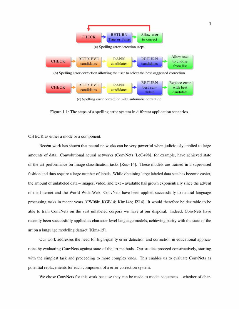
The steps a spelling error system takes in common application scenarios are shown in Figure 1.1:

Figure 1.1a has the requisite steps for error detection alone; Figure 1.1b has the steps for error correction

that delegates responsibility for choosing the correct suggestion to the user; and the steps the system takes

when performing automated correction are in Figure 1.1c. The final step (shown in green) is the responsibil-

ity of the application interacting with the spelling system; it is shown here to provide context. Throughout

this thesis we refer to these scenarios as modes of a spelling error system – respectively, CHECK, SUG-

GEST, and CORRECT. We refer to each step as a component of a spell checking system. The components

identified in Figure 1.1 are CHECK, RETRIEVE, RANK, and RETURN; for clarity, we qualify uses of

3

CHECK RETURNTrue or False

Allow userto correct

(a) Spelling error detection steps.

CHECK RETRIEVEcandidates

RANKcandidates

RETURNcandidates

Allow userto choosefrom list

(b) Spelling error correction allowing the user to select the best suggested correction.

CHECK RETRIEVEcandidates

RANKcandidates

RETURNbest can-

didate

Replace errorwith bestcandidate

(c) Spelling error correction with automatic correction.

Figure 1.1: The steps of a spelling error system in different application scenarios.

CHECK as either a mode or a component.

Recent work has shown that neural networks can be very powerful when judiciously applied to large

amounts of data. Convolutional neural networks (ConvNet) [LeC+98], for example, have achieved state

of the art performance on image classification tasks [Rus+14]. These models are trained in a supervised

fashion and thus require a large number of labels. While obtaining large labeled data sets has become easier,

the amount of unlabeled data – images, video, and text – available has grown exponentially since the advent

of the Internet and the World Wide Web. ConvNets have been applied successfully to natural language

processing tasks in recent years [CW08b; KGB14; Kim14b; JZ14]. It would therefore be desirable to be

able to train ConvNets on the vast unlabeled corpora we have at our disposal. Indeed, ConvNets have

recently been successfully applied as character-level language models, achieving parity with the state of the

art on a language modeling dataset [Kim+15].

Our work addresses the need for high-quality error detection and correction in educational applica-

tions by evaluating ConvNets against state of the art methods. Our studies proceed constructively, starting

with the simplest task and proceeding to more complex ones. This enables us to evaluate ConvNets as

potential replacements for each component of a error correction system.

We chose ConvNets for this work because they can be made to model sequences – whether of char-

4

acters or words – well. In this regard they resemble probabilistic language models, the simplest forms of

which count the occurrences of sequences in a corpus in order to obtain the probability that an atom (a char-

acter or word) t follows a sequence t−n, . . . , t−2, t−1 of atoms. Two key differences between probabilistic

language models and ConvNets as they are used in this thesis are (1) probabilistic language models embed

atoms in a disjoint, categorical space, whereas ConvNets embed them in an overlapping, continuous space;

and (2) probabilistic language models are unsupervised, whereas ConvNets are supervised. To highlight the

performance implications of these differences, we contrast ConvNets and probabilistic language models in

a number of studies – specifically, those in Chapters 3, 4, and 5.

1.2 Problems and Contributions

In this section we discuss the research problems our work addresses and our work’s contributions.

1.2.1 Non-word Error Detection

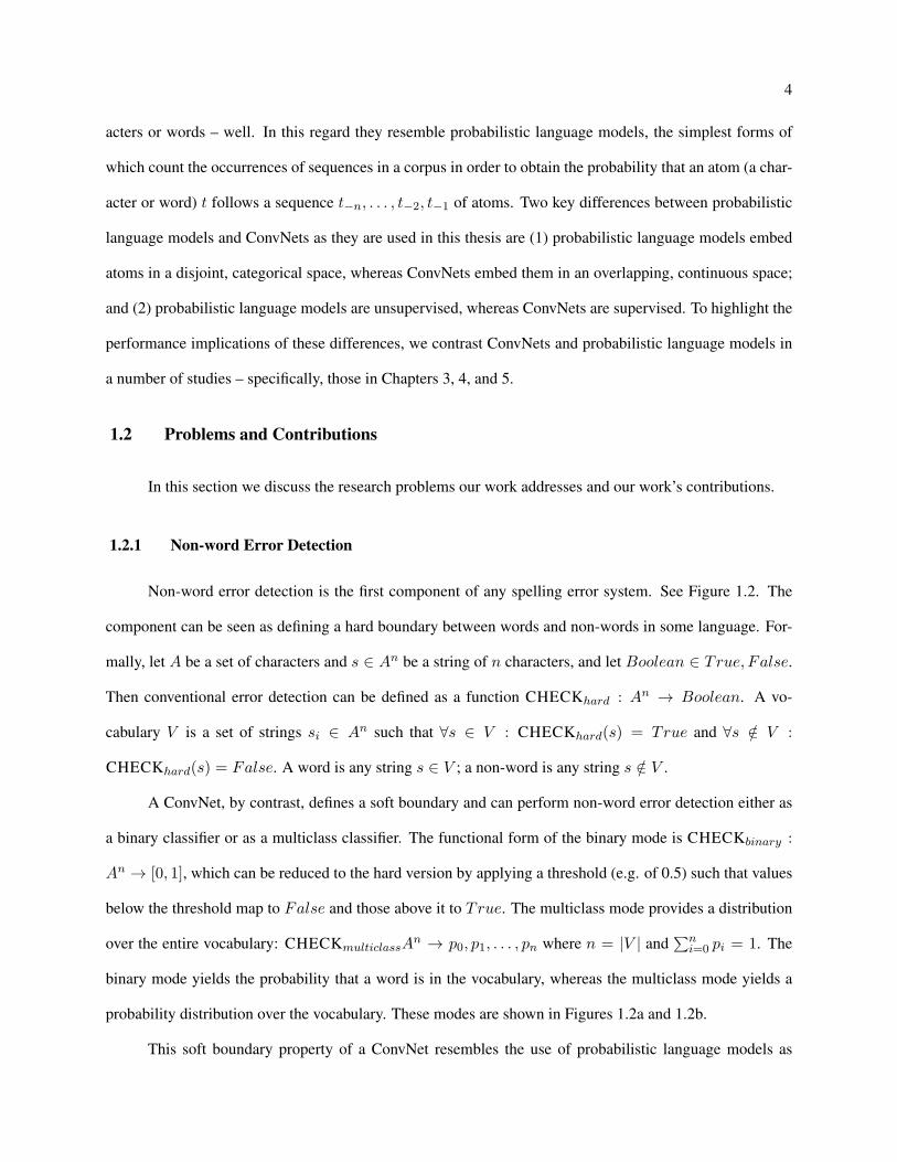
Non-word error detection is the first component of any spelling error system. See Figure 1.2. The

component can be seen as defining a hard boundary between words and non-words in some language. For-

mally, let A be a set of characters and s ∈ An be a string of n characters, and let Boolean ∈ True, False.

Then conventional error detection can be defined as a function CHECKhard : An → Boolean. A vo-

cabulary V is a set of strings si ∈ An such that ∀s ∈ V : CHECKhard(s) = True and ∀s /∈ V :

CHECKhard(s) = False. A word is any string s ∈ V ; a non-word is any string s /∈ V .

A ConvNet, by contrast, defines a soft boundary and can perform non-word error detection either as

a binary classifier or as a multiclass classifier. The functional form of the binary mode is CHECKbinary :

An → [0, 1], which can be reduced to the hard version by applying a threshold (e.g. of 0.5) such that values

below the threshold map to False and those above it to True. The multiclass mode provides a distribution

over the entire vocabulary: CHECKmulticlassAn → p0, p1, . . . , pn where n = |V | and∑n

i=0 pi = 1. The

binary mode yields the probability that a word is in the vocabulary, whereas the multiclass mode yields a

probability distribution over the vocabulary. These modes are shown in Figures 1.2a and 1.2b.

This soft boundary property of a ConvNet resembles the use of probabilistic language models as

5

couldcourse

cood

coude couled

courscource

corce

(a) Non-word error detection as binary classification. Thewords in the vocabulary are members of one class (green);

non-words are members of another (red).

could

coodcoude

colud couled

kudcourse

corse

cose

cours

courcecorcecort

(b) Non-word error detection as multiclass classification.Each word in the vocabulary is a member of its own class

(here, green and blue); non words are members of thesame class (red).

Figure 1.2: When used for non-word error detection, a ConvNet can function either as a binary or a multi-class classifier.

6

classifiers. Consider two character-level language models, one (LM1) trained on real words from a language,

the other (LM2) trained on spelling errors in that language. When presented a word w, LM1 will give the

probability that w is in the language and LM2 will give a probability that it is not. An important question

is, then, whether and how a ConvNet binary classifier trained to distinguish words from non-words differs

from a pair of language models trained to do the same thing.

1.2.2 Isolated Non-word Error Correction

Proceeding constructively, we next consider the use of ConvNets for isolated non-word error cor-

rection. In a spelling error system, this correction task is comprised of the components RETRIEVE and

RANK. Given a non-word s ∈ An, RETRIEVE is responsible for finding a set of real words w ∈ V such

that s is a plausible misspelling of w, and RANK is responsible for rearranging the set of retrieved words

according to some partial order χ : s ∈ An ×wy ∈ V ×wz ∈ V → R such that χ(s, wa, wb) ≤ χ(s, wb, wa)

if wa is a better replacement for s than wb:

The functional forms of the components are

RETRIEVE :s ∈ An → w1, w2, . . . , wm

RANK :s ∈ An × w1, w2, . . . , wm → wr1 , wr2 , . . . , wrm

where wi is the i-th retrieved word, m is the number of words retrieved, and wrkis the word in the k-th

position implied by Ξ. Note that RANK takes both the error s and the set of candidates, which means that

the best replacement for a given s may be conditioned on s itself.

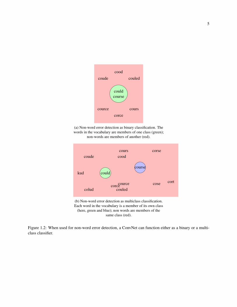
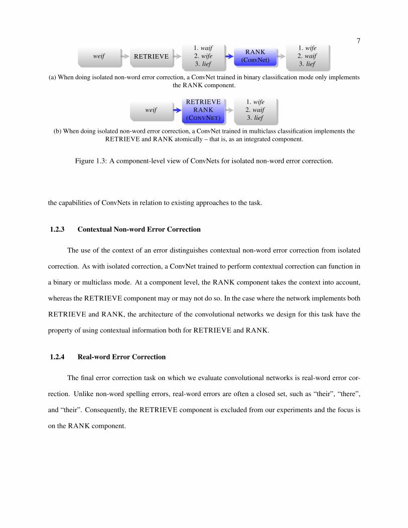
For this task, as with non-word error detection, a ConvNet can function in a binary or a multiclass

mode, as shown in Figures 1.3a and 1.3b. In binary mode, the ConvNet only implements RANK, and

RETRIEVE is an external component. In multiclass mode, it implements both RETRIEVE and RANK

in a single component. An expected advantage of using ConvNets – regardless of the chosen mode of

classification – for non-word error correction is their ability to detect soft features.

In this thesis we evaluate ConvNets trained in binary and multiclass classification modes on the task

of isolated non-word error correction. We compare our models to strong baselines in order to understand

7

weif RETRIEVE1. waif2. wife3. lief

RANK(ConvNet)

1. wife2. waif3. lief

(a) When doing isolated non-word error correction, a ConvNet trained in binary classification mode only implementsthe RANK component.

weifRETRIEVE

RANK(CONVNET)

1. wife2. waif3. lief

(b) When doing isolated non-word error correction, a ConvNet trained in multiclass classification implements theRETRIEVE and RANK atomically – that is, as an integrated component.

Figure 1.3: A component-level view of ConvNets for isolated non-word error correction.

the capabilities of ConvNets in relation to existing approaches to the task.

1.2.3 Contextual Non-word Error Correction

The use of the context of an error distinguishes contextual non-word error correction from isolated

correction. As with isolated correction, a ConvNet trained to perform contextual correction can function in

a binary or multiclass mode. At a component level, the RANK component takes the context into account,

whereas the RETRIEVE component may or may not do so. In the case where the network implements both

RETRIEVE and RANK, the architecture of the convolutional networks we design for this task have the

property of using contextual information both for RETRIEVE and RANK.

1.2.4 Real-word Error Correction

The final error correction task on which we evaluate convolutional networks is real-word error cor-

rection. Unlike non-word spelling errors, real-word errors are often a closed set, such as “their”, “there”,

and “their”. Consequently, the RETRIEVE component is excluded from our experiments and the focus is

on the RANK component.

8

1.2.5 Generative Spelling Error Model

Data acquisition is a challenge when training statistical models to correct errors. The studies in this

thesis involve the use of a high-variance model, which can require a large number of labeled examples to

generalize well. Since, on the whole, errors are relatively infrequent, obtaining a large corpus of errors and

corrections requires substantial effort.

For our studies of spelling errors, we propose to circumvent this difficulty by learning how to generate

examples of non-words. We accomplish this by learning patterns of misspellings from relatively small

corpora of errors and corrections. The patterns can then be used to edit real words into non-words that

mimic the errors people make. The patterns are sampled with probability proportional to their frequency in

the corpora of real errors.

1.3 Report Summary and Organization

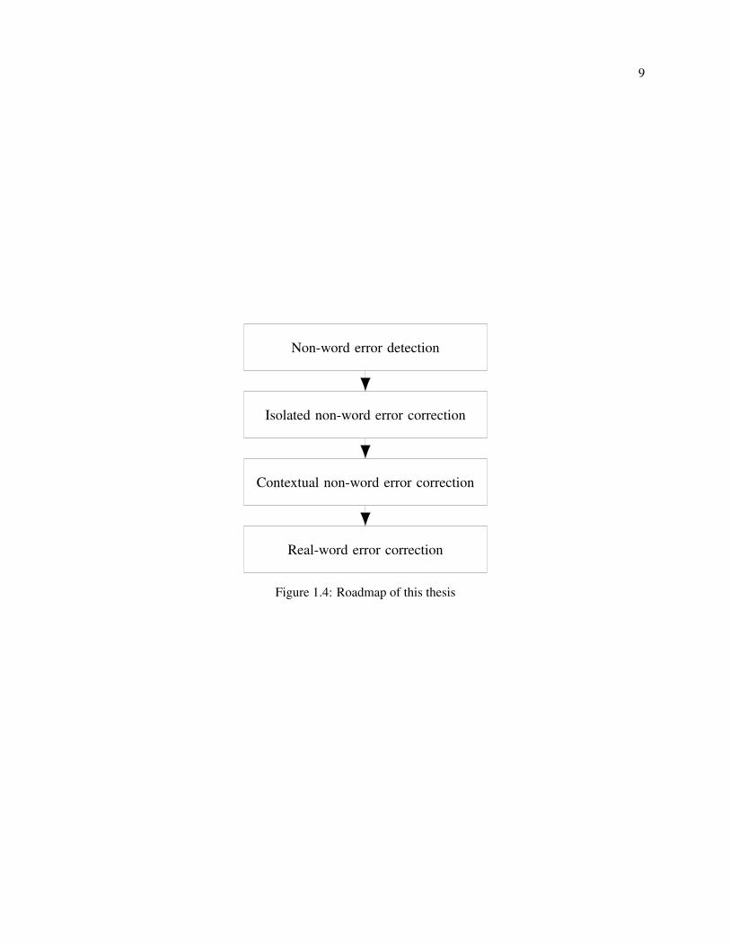
A road map of this thesis is shown in Figure 1.4. In the rest of this chapter, we review notation and

terminology (Section 1.4) and describe the research questions we pursue (Section 1.5). The rest of this thesis

is organized as follows. In Chapter 2 we review the relevant literature. We study convolutional networks

on the non-word error detection task in Chapter 3. Chapters 4, 5, and 6 evaluate convolutional networks

on correction tasks, including isolated non-word error correction, contextual non-word error correction, and

real-word error correction. Chapter 7 concludes.

9

Non-word error detection

Isolated non-word error correction

Contextual non-word error correction

Real-word error correction

Figure 1.4: Roadmap of this thesis

10

1.4 Notation and Terminology

1.4.1 Notation

In this thesis, matrices M ∈ Rn×m are denoted in bold script. The ith row of a matrix M is M(i),

the jth column is Mj , and the jth entry of the ith row is M(i)j . An element-wise non-linear transformation

is denoted as σ.

1.4.2 Terminology

1.4.2.1 Neural network

A neural network is a sequence of non-linear transformations, or layers. Let the L be the number of

layers in a network. The layers of a network are labeled l ∈ 1 . . . L. A typical layer consists of a linear

transformation followed by the element-wise application of a non-linear function. Conventionally this is

represented as σ(Wlx + bl), where Wl1 and bl are the weights and biases of layer l, respectively, and x is

the input.

The weights of a network are usually randomly initialized. They are then trained by feeding train-

ing examples forward through the network, then computing a loss function using the output of the final

layer, which is propagated backwards through the layers to change the weights in accordance with their

contribution to the loss incurred at the output layer.

1.4.2.2 Convolutional Neural Network (ConvNet)

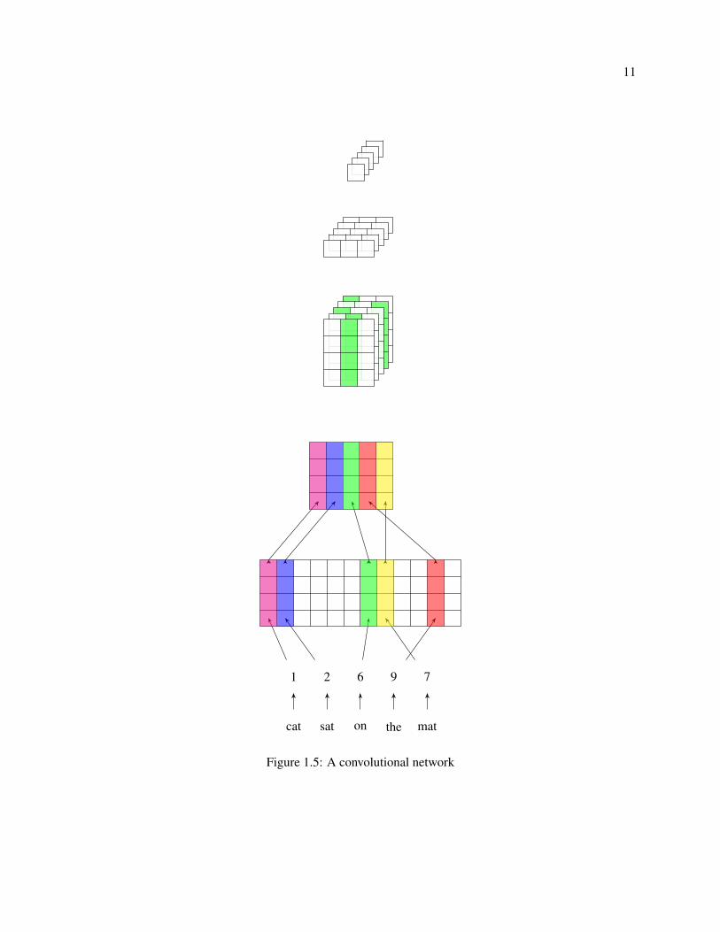
Here we describe the components of a ConvNet trained for natural language processing tasks. Such

a network has a word embedding layer followed by one or more convolutional and pooling layers. Those in

turn are followed by zero or more fully-connected layers, then an output layer.

The input to the network is a fixed-width vector representing a sequence of words. Here we are

modeling sentences, so the width of a training example is the number of words in the longest sentence of

the training set. The elements of an input sentence vector are the indices in the vocabulary of the words in

the sentence.

11

cat sat on the mat

1 2 6 9 7

Figure 1.5: A convolutional network

12

Distributed word representations

Each word in the vocabulary has a corresponding row in the weight matrix of this layer. Each row thus

has a distributed representation of a word. This layer takes as input a vector of indices into the vocabulary.

Each index is used to look up the distributed representation that occurs at that position in the sentence. The

word representations are then concatenated into a matrix with one column for each position in the sentence

and one row for each dimension of the word representation.

Some options available to the network designer are whether to initialize this layer’s weights randomly

or with pre-trained word representations (e.g. [Mik+13b]). If the latter, one must also choose whether to

allow the weights to be updated by backpropagation when the network is being trained.

Discrete convolution

A convolutional layer consists of one or more filters. With a ConvNet trained for a natural language

processing task, a filter is a 3-tensor. One of the tensor’s dimensions is the number of filters, the other two

are the number of rows and columns in a filter. If the number of columns of a filter matches the number of

dimensions of the word embeddings, we say that the filter spans the word embeddings.

The convolutional operation for the ith filter in layer l is given by:

σ(Wl,i ∗ x + bl), (1.1)

where ∗ is the convolutional operation.

Pooling

Convolutional layers are usually followed by a pooling layer (sometimes called a subsampling layer).

The pooling layer takes the maximum value over the region of the output of the convolutional layer. This

reduces the dimensionality of the output of one layer.

1.5 Research Questions

1.5.1 Research Question 1

The detection of spelling errors is the first component in any spelling error system. It would thus

be of interest to understand the characteristics of a ConvNet trained to perform non-word error detection.

13

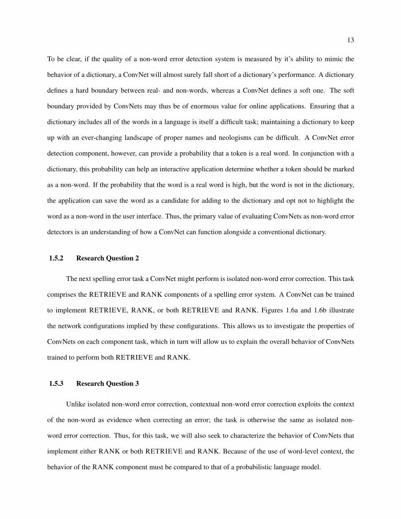
To be clear, if the quality of a non-word error detection system is measured by it’s ability to mimic the

behavior of a dictionary, a ConvNet will almost surely fall short of a dictionary’s performance. A dictionary

defines a hard boundary between real- and non-words, whereas a ConvNet defines a soft one. The soft

boundary provided by ConvNets may thus be of enormous value for online applications. Ensuring that a

dictionary includes all of the words in a language is itself a difficult task; maintaining a dictionary to keep

up with an ever-changing landscape of proper names and neologisms can be difficult. A ConvNet error

detection component, however, can provide a probability that a token is a real word. In conjunction with a

dictionary, this probability can help an interactive application determine whether a token should be marked

as a non-word. If the probability that the word is a real word is high, but the word is not in the dictionary,

the application can save the word as a candidate for adding to the dictionary and opt not to highlight the

word as a non-word in the user interface. Thus, the primary value of evaluating ConvNets as non-word error

detectors is an understanding of how a ConvNet can function alongside a conventional dictionary.


The next spelling error task a ConvNet might perform is isolated non-word error correction. This task

comprises the RETRIEVE and RANK components of a spelling error system. A ConvNet can be trained

to implement RETRIEVE, RANK, or both RETRIEVE and RANK. Figures 1.6a and 1.6b illustrate

the network configurations implied by these configurations. This allows us to investigate the properties of

ConvNets on each component task, which in turn will allow us to explain the overall behavior of ConvNets

trained to perform both RETRIEVE and RANK.


Unlike isolated non-word error correction, contextual non-word error correction exploits the context

of the non-word as evidence when correcting an error; the task is otherwise the same as isolated non-

word error correction. Thus, for this task, we will also seek to characterize the behavior of ConvNets that

implement either RANK or both RETRIEVE and RANK. Because of the use of word-level context, the

behavior of the RANK component must be compared to that of a probabilistic language model.

14

c o m p l e t l y c o m p l e t e l y

Em

bedd

ings

Filte

rout

puts

Pool

outp

uts

Con

volu

tiona

lfilte

rsSo

ftm

ax

(a) A hypothetical binary classification ConvNet that functions as a RANK component for isolated non-word errorcorrection. It takes the spelling error and a suggested replacement as input. The output of the network is a probability

that is used to rank suggested replacements.

c o m p l e t l y

. . . . . .

Em

bedd

ings

Filte

rout

puts

Pool

outp

uts

Con

volu

tiona

lfilte

rsSo

ftm

ax

(b) A hypothetical multiclass classification ConvNet that functions either only as the RETRIEVE component or asboth the RETRIEVE and the RANK components for isolated non-word error correction. It takes the spelling erroras input. The output of the network is a probability distribution over the words in the vocabulary. The words with

non-zero probability are the retrieved words and their partial order is their ranking.

Figure 1.6: Convolutional network architectures for isolated non-word error correction.

15

c o m p l e t l y

they

just

com

plet

ely

igno

reev

eryt

hing

Em

bedd

ings

Filte

rout

puts

Pool

outp

uts

Con

volu

tiona

lfilte

rsSo

ftm

ax

(a) A hypothetical binary classification ConvNet that functions as a RANK component for contextual non-word errorcorrection. It takes the spelling error, a suggested replacement, and the context of the error as input. The output of the

network is a probability that is used to rank suggested replacements.

c o m p l e t l y

they

just

igno

reev

eryt

hing

. . . . . .

Em

bedd

ings

Filte

rout

puts

Pool

outp

uts

Con

volu

tiona

lfilte

rsSo

ftm

ax

(b) A hypothetical multiclass classification ConvNet that functions either only as the RETRIEVE component or asboth the RETRIEVE and the RANK components for contextual non-word error correction. It takes the spelling

error and the context of the error as input. The output of the network is a probability distribution over the words in thevocabulary. The words with non-zero probability are the retrieved words and their partial order is their ranking.

Figure 1.7: Convolutional network architectures for contextual non-word error correction.

16


conc

ert

was

quie

tlo

udto

nigh

t

. . . . . .

Em

bedd

ings

Filte

rout

puts

Pool

outp

uts

Con

volu

tiona

lfilte

rsSo

ftm

ax

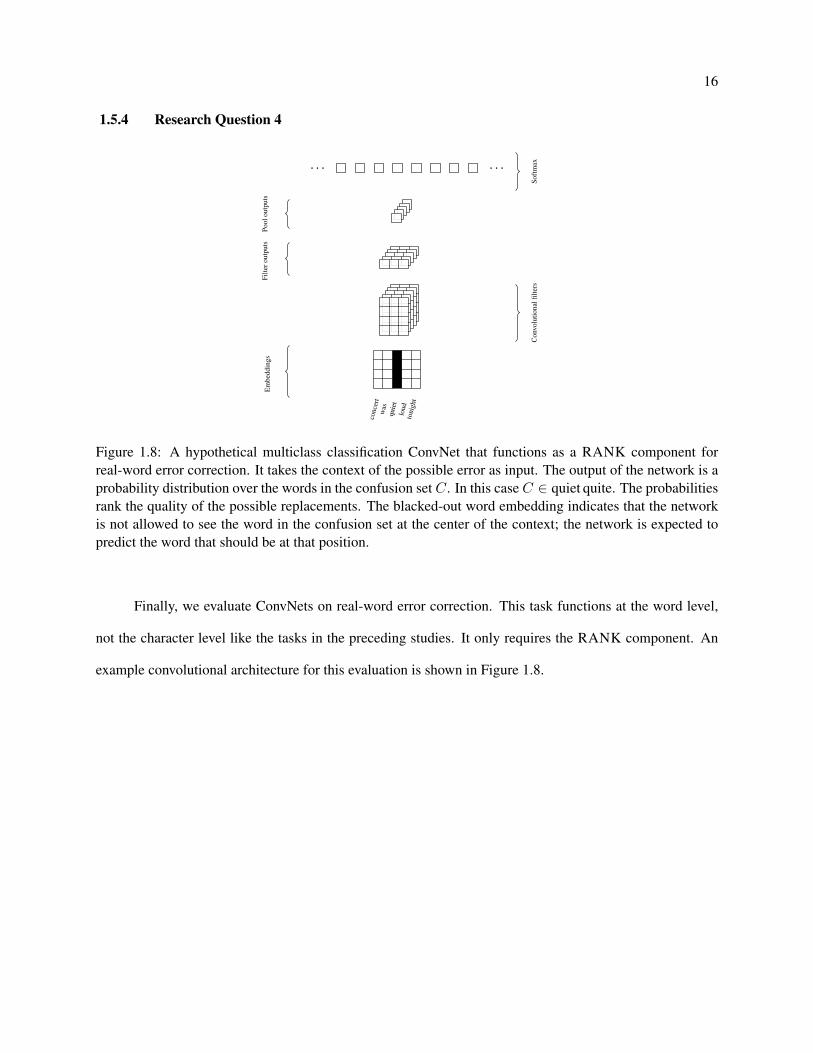
Figure 1.8: A hypothetical multiclass classification ConvNet that functions as a RANK component forreal-word error correction. It takes the context of the possible error as input. The output of the network is aprobability distribution over the words in the confusion set C. In this case C ∈ quiet quite. The probabilitiesrank the quality of the possible replacements. The blacked-out word embedding indicates that the networkis not allowed to see the word in the confusion set at the center of the context; the network is expected topredict the word that should be at that position.

Finally, we evaluate ConvNets on real-word error correction. This task functions at the word level,

not the character level like the tasks in the preceding studies. It only requires the RANK component. An

example convolutional architecture for this evaluation is shown in Figure 1.8.

Chapter 2

Literature Review

2.1 Spelling Error Detection and Correction

In this section we review the relevant spelling error detection and correction literature. The terms we

use for types of errors – non-word and real word errors – and the types of task – non-word error detection,

isolated non-word error correction, and context-dependent non-word or real word error correction – follow

the terms in the survey by Kukich [Kuk92b].

Empirical studies of spelling errors have yielded an understanding of the types of errors and how often

they occur in relation to others. Kukich describes three types of non-word errors: (1) typographic errors,

(2) cognitive errors, and (3) phonetic errors [Kuk92b]. Typographic errors occur because of the physical

interaction of a person and a keyboard, not because the person doesn’t know how to spell a word. (As an

example, in the process of writing the previous sentence, the author wrote “pearson” – his employer’s name

lower-cased – instead of “person” three times. This typographic error resulted because of the similarity of

“pearson” and “person” and because the author is accustomed to typing his employer’s name in emails.)

A cognitive error occurs when the writer can reliably spell a given word, but accidentally makes an error

with that word because of a transient mental state. An an example, one may intend to write “house” but

instead write “horse” because “horse” was just overheard in a conversation. Phonetic errors are due to lack

of knowledge of morphology.

Mitton showed that typographic and phonetic errors can be distinguished based on the similarity of

the non-word to the correct word [Mit87]. Typographic errors tend to be quite similar to the correct word.

Phonetic errors, on the other hand, tend to differ more drastically from the correct word; according to Mitton,

18

“knowledge of pronunciation would help in correcting many of [these] errors, but misspellings do not always

reflect pronunciation in a simple way”. One study reports that most spelling errors differ from the correct

word by one character [PZ84].

2.1.1 Non-word Error Detection

Some approaches to non-word error detection do not rely on a fixed dictionary of real words. Instead,

they make use of the document in which the words appear. These are spelling checking programs that take

a document as input and use the characteristics of the document as a whole to identify the words that are

more likely to be non-words.

Two questions lie at the heart of non-word error detection. One is motivated by the need for computers

to respond expeditiously to human queries: given a list of real words, what data structures and algorithms

allow a machine to determine quickly whether a query word is in the dictionary? There is a clear answer in

the computer science literature in the form of the dictionary. A dictionary is an abstract data type (ADT) that

supports the operations INSERT, DELETE, and MEMBER. Efficient implementations of each operation

are enabled by hashing. A function h that performs hashing can be defined as h : s ∈ An → Z+, where s

is a string, A is an alphabet, n is a free length. The time complexity of efficient hashing functions is O(1),

assuming n is bounded from above. The integer output of a hashing function allows strings to be associated

with fixed positions in an array. If an empty linked list – or “bucket” – is stored at each position in an array,

then using the INSERT operation to add a new word to a dictionary requires an O(2) hashing operation and

an O(1) insertion at the head of the linked list. If the linked list is not empty, appending to the list is also

a O(1) operation. Assuming a simple linked list implementation, the DELETE and MEMBER operations

are O(m). It is thus important that each linked list is kept as short as possible or, concomitantly, that the

hashing function minimizes collisions, which occur when multiple inputs hash to the same bucket. Efficient

dictionary implementations thus depend on good hashing functions. A canonical review of the dictionary

ADT can be found in [HUA83].

The other question for non-word error detection is: which words should be included? This is a serious

issue for dictionary implementers. A comprehensive dictionary such as the Oxford English Dictionary has

19

on the order of two hundred and fifty thousand entries. Is a dictionary with a vocabulary of that size useful

for detecting spelling errors? A dictionary with too few words will result in many false positives. A larger

vocabulary will decrease the false positive rate at the cost increasing the false negative rate. Mitton raised

the issue that care must be taken in handling rare words, some of which happen to be misspellings of

common ones [Mit10]. The common word calendar can be misspelled calender, because of how the final a

is pronounced, and calender happens to be a real word that refers to a roller for pressing cloth.

2.1.2 Isolated Non-word Error Correction

Approaches to the isolated non-word error correction task are conventionally based on some definition

of distance between a given non-word and a candidate real word. Here we consider distances between

strings, distances between vector-space embeddings of n-grams of strings, phonetic matching techniques,

approaches that employ finite-state automata, corpus-based techniques, and – more generally – attempts to

model spelling errors.

2.1.2.1 String Distance Techniques

String distance approaches posit a distance d(s, s′) between strings s and s′. Perhaps the earliest

string distance is Hamming distance, which simply measures the number of differences between two equal-

length binary strings [Ham50]. Because it is restricted to equal-length binary strings, it is of limited utility

with strings; it has, however, been seen to be of some use in the vector-space approaches described in the

next section.

The Damerau-Levenshtein distance between s and s′ is the number of character insertions, deletions,

substitutions, and transpositions required to transform s into s′ [Dam64a]. Closely related to Damerau-

Levenshtein distance is Levenshtein distance [Lev66] which excludes transpositions. Because s and ′s are

not required to be of equal length, both Damerau-Levenshtein distance and Levenshtein distance are widely

used for natural language processing tasks, including non-word error correction. A

Record linkage is the task of linking entities across heterogeneous data sets where misspellings may

occur. The intent is to find all of the records for a particular entity, despite accidental variation in e.g. spelling

20

of proper names. This is a particular problem for organizations that need to combine records. Jaro and Jaro-

Winkler distance originated in the record linkage literature. Jaro distance is a function of (1) the number

of characters that are in both s and s′ within a window of characters and (2) the number of transpositions

[Jar89].

There is a common notion that misspellings are relatively less frequent at the beginning of a word

than elsewhere. There are some counterexamples, such as “cicolagie” or “sicolagee” – both misspellings

of “psychology” – and the literature is mixed about this. The reported rates of first-position errors includes

1.4% (of 568 errors) [YF83], 3.3% (of 50,000 errors) [PZ83], 7% [Mit87], and 15% (of 40,000 examples)

[Kuk92a]. Regardless, Jaro-Winkler distance enhances Jaro distance by giving a bonus when s and s′ start

with the same characters; the bonus is proportional to the length of the matching prefix [Win90].

A string distance technique for finding all words with a Damerau-Levenshtein distance ≤ 2 from a

given non-word is described by Peterson [Pet80]; it is sometimes referred to as the near-miss technique. The

technique effectively implements a string-distance form of a dictionary’s RETRIEVE component. It starts

by generating a set of variations of the non-word by applying every possible insertion, deletion, substitution,

and transposition. The Damerau-Levensthein distance from the resulting strings to the original non-word is

1. Applying this procedure again yields a set of strings with Damerau-Levenshtein distance 2 from the non-

word. The two sets can then be checked against the dictionary to eliminate the non-words. The resulting

set of real words constitutes the candidate list. The set of characters used for insertion and substitution

includes the letters in the English alphabet. Insertion also includes the space and the hyphen; these allow the

search process to account for the possibility that the non-word is the concatenation of real words. Finding

words with Damerau-Levenshtein distance > 2 is time consuming, as the number of candidates increases

supralinearly, so this technique is usually only used for distances ≤ 2.

Words vary in length, which is why Hamming distance isn’t an effective measure of distances between

non-words and real words. The string distances described in this section work even when s and s′ are of

different length because they approach the task as an alignment problem. They operate on strings as though

they have a beginning, a middle, and an end, which is appropriate, because they do.

21

2.1.2.2 Vector-space Distance Techniques

Another way to measure the distance between a non-word s and a candidate word s′ is to embed s

and s′ into a D-dimensional vector space as v⃗ and v⃗′, where D is the number of dimensions. The distance

between s and s′ can then be computed as the distance between the feature vectors v⃗ and v⃗′. The feature

vectors may be the n-grams (1, 2, or 3, typically) of each word in the dictionary. A dictionary’s CHECK

component can be implemented by obtaining the feature vector u⃗ for some query and searching the neigh-

borhood of u⃗; if there is a vector u⃗′ such that the distance between u⃗ and u⃗′ is 0, then CHECK returns

true. Similarly, the RETRIEVE component can be implemented by returning the k words that correspond

to the vectors in the neighborhood of u⃗, for some cutoff k, and RANK can be implemented by sorting the

retrieved words in increasing order of the distance of their vectors from u⃗. This approach was tried by Ku-

kich [Kuk92a] using Hamming distance, dot product, and cosine distance, and reported accuracies of 54%

for dot product, 68% for Hamming distance, and 75% for cosine distance over a baseline of 62% for a string

distance technique called grope.

2.1.2.3 Phonetic Matching Techniques

In a previous section we mentioned record linkage. A goal of record linkage to join records across

heterogeneous databases. A person’s name may be spelled slightly differently in each database due to

clerical typographic or cognitive errors. A string distance such as Jaro-Winkler distance can be used to find

proximal names. Phonetic matching is another tool that can be used for record linkage, and it is also useful

for non-word error correction. The idea is to encode words in such a way that homophones receive the

same code. Examples of phonetic matching algorithms are Soundex [RO18], NYSIIS [Taf70], Metaphone

[Phi90], and Double Metaphone [Phi00].

Encodings produced by Soundex, NYSIIS, and Double Metaphone are shown in Table 2.1. A weak-

ness of Soundex can be seen with “kake”; because the algorithm preserves the initial character, the phonetic

matching code differs from that of “cake”. Both NYSIIS and Double Metaphone encode “cake” and “kake”

the same. Unsurprisingly, the codes produced for wildly different strings like “psychology” and “cicollegy”

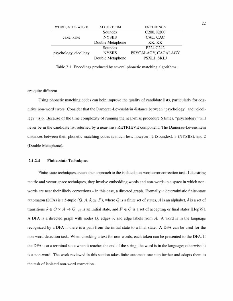
22WORD, NON-WORD ALGORITHM ENCODINGS

cake, kakeSoundex C200, K200NYSIIS CAC, CAC

Double Metaphone KK, KK

psychology, cicollegySoundex P224,C242NYSIIS PSYCALAGY, CACALAGY

Double Metaphone PSXLJ, SKLJ

Table 2.1: Encodings produced by several phonetic matching algorithms.

are quite different.

Using phonetic matching codes can help improve the quality of candidate lists, particularly for cog-

nitive non-word errors. Consider that the Damerau-Levenshtein distance between “psychology” and “cicol-

legy” is 6. Because of the time complexity of running the near-miss procedure 6 times, “psychology” will

never be in the candidate list returned by a near-miss RETRIEVE component. The Damerau-Levenshtein

distances between their phonetic matching codes is much less, however: 2 (Soundex), 3 (NYSIIS), and 2

(Double Metaphone).

2.1.2.4 Finite-state Techniques

Finite-state techniques are another approach to the isolated non-word error correction task. Like string

metric and vector-space techniques, they involve embedding words and non-words in a space in which non-

words are near their likely corrections – in this case, a directed graph. Formally, a deterministic finite-state

automaton (DFA) is a 5-tuple (Q, A, δ, q0, F ), where Q is a finite set of states, A is an alphabet, δ is a set of

transitions δ ∈ Q × A → Q, q0 is an initial state, and F ∈ Q is a set of accepting or final states [Hop79].

A DFA is a directed graph with nodes Q, edges δ, and edge labels from A. A word is in the language

recognized by a DFA if there is a path from the initial state to a final state. A DFA can be used for the

non-word detection task. When checking a text for non-words, each token can be presented to the DFA. If

the DFA is at a terminal state when it reaches the end of the string, the word is in the language; otherwise, it

is a non-word. The work reviewed in this section takes finite automata one step further and adapts them to

the task of isolated non-word correction.

23

Oflazer [Ofl96] proposed an error-tolerant finite-state recognizer that would yield a list of candidate

corrections when presented a non-word. Since a DFA will be in a non-terminal state when it reaches the

end of the string of a non-word, a candidate list can be generated by finding all paths from the initial

state to plausible terminal states. Doing this efficiently requires avoiding taking paths that correspond to

words that are greater than a given edit distance from the non-word, which Oflazer refers to as the cut-

off edit distance. The cut-off edit distance is computed as the algorithm traverses the graph depth first,

and the program backtracks whenever the cut-off edit distance is exceeded or no transitions are possible.

This algorithm was used as a component in a system for learning morphological analyzers with little human

annotation[ONM01]. More efficient versions or variants of this algorithm for generating candidate lists have

been proposed [Sav01; SM02; MS04]. In Section 2.1.3 we summarize a study that evaluated the Oflazer

algorithm on the context-dependent non-word correction task [HNH08].

2.1.2.5 Corpus-based Techniques

Corpus-based techniques exist somewhere between isolated non-word correction and context-dependent

non-word correction. They take advantage of some context, which distinguishes them from isolated non-

word correction techniques. Yet, unlike context-dependent non-word correction techniques, the context they

exploit is not the immediate, local context of a non-word but the global context of a corpus. For instance,

ranking the words in a candidate list by their proximity to the non-word may not produce the optimal rank-

ing. If we are attempting to correct “hve”, and if the true correction is “have”, it is possible for the first

candidate to be “hove” because it and “have” are equidistant from “hve”. This can be improved by sorting

the candidate list by distance, truncating the list to the top k candidates, then sorting by word frequency

using counts obtained from some corpus. Probabilistically, this is can be seen as a simple language model

approach that arranges the truncated candidate list words w by P (w). In introducing the concept of a

corpus-based technique, we diverge from the terminology of Kukich [Kuk92b].

Morris described a program for identifying likely spelling errors [MC75] by using a document to fit

a bigram and trigram character language model. The program uses the character language model to find

words containing unlikely character sequences. Since this approach does not require a dictionary, it can be

24

applied to documents of varying languages without significant modification.

Yannakoudakis and Fawthrop sought to discover the regularities in spelling errors [YF83]. They

considered two corpora: a corpus of 809 typical errors discovered gathered from previous research about

spelling errors [Las41; Dam64b; KF67; Mas27]; and a corpus of 568 errors obtained from three adults

who identified themselves as poor spellers. They provide a detailed analysis of the consonantal, vowel, and

sequential errors for both corpora. They found a correlation between non-words and the errors that cause

them: the more frequent a non-word, the more frequent the error.

A noisy channel model for correcting non-word errors was introduced [KCG90]. The noisy channel

model is a probabilistic model of the process of generating a non-word w′ from a real word w. The model

can be obtained by starting with a corpus of spelling errors and corrections. The edit operation required

to transform each correction w into the corresponding error w′ is recorded, and the counts of the opera-

tions are recorded. Ranking the candidate list by sorting the words w in descending order of probability

P (w)P (w′|w) was reported to yield good rankings. The effectiveness of this model corroborates the find-

ing of Yannakoudakis and Fawthrop [YF83] that the frequency of a non-word is related to the frequency of

the error that causes it.

Brill and Moore refined the noisy channel model P (w′|w) by introducing a more generic model of

character-level edits from w to w′ [BM00]. Toutanova explored improving the noisy channel model further

by learning a model of phonetic errors and combining it with the generic character-level model [TM02].

On a test set of 1,812 examples of spelling errors and corrections, the top-1 accuracies of the original, the

generic character-level, and the combined character-phoneme noisy channel models were 89.5%, 93.6%,

and 95.58%, respectively.

The work surveyed in this section serves as background for the generative model of non-words that

we introduce in Section 4.1.0.2. Our generative model most closely resembles the noisy channel model

[KCG90], with the key difference that ours is the first generative use of the noisy channel model. In prior

work, the noisy channel model has been used as a scoring function for ranking candidate lists.

25

2.1.3 Context-dependent Correction

In this section we review techniques that make use of the immediate context of an error; the techniques

apply both to non-word and real word errors. Correcting non-word errors without exploiting the context of

the error results in levels of accuracy that vary from modest to high, depending on the severity of the errors in

an error corpus. A non-word on its own only provides so much information; a non-word’s context contains

additional clues and exploiting it can improve non-word error correction significantly. Real word errors –

writing there or their instead of they’re, for example – can only be fixed by considering the context of the

real word.

Real word errors may be typographic or cognitive. A typographic real word error is a typographic

error that happens to result in one real word being typed as another real word, such as typing “house” when

“horse” was intended. A cognitive real word error occurs when the writer uses the incorrect word because

of a momentary lapse – such as typing “they’re” instead of ”their” – or because of a poor understanding of

vocabulary – such as using “affect” instead of “effect”. A characteristic of cognitive real word errors is that

the misused word is often phonetically nearly identical to the correct word.

A notable early analysis of real word errors was done by Peterson [Pet86]. To estimate the probability

of making typographic real word error, he created all possible single-operation edits to the words in a

dictionary of 369,546 words. Each edit to a real word resulted in a possible, other real word. Of all the

words in the dictionary, 153,664 could not be turned into another real word by a single edit operation. Of

the remaining, there were 988,192 pairs of real words that could be transformed into one another by an

operation. Conditioned on the type of error, the error frequencies were:

616,210 Substitution

180,559 Insertion

180,559 Deletion

10,864 Transposition

Gale and Church discovered that when humans judge spelling corrections, they are much more con-

fident in their judgments when provided some of the context of the non-word. They showed that using an

26

n-gram language model with Good-Turing smoothing is an effective way to achieve improvement in non-

word error correction [GC90; CG91]. The basic approach is to use the language model to obtain an estimate

of the probability of a non-word’s context when the non-word has been replaced by a real word from a

candidate list of corrections. Mays, Damerau, and Mercer [MDM91] employed an approach similar to that

of Gale and Church but evaluated their system on real word instead of non-word errors. Their empirical

evaluation showed an error detection rate of 76% and a correction rate of 73%.

Yarowsky used syntactic and semantic contextual features to restore missing accents in Spanish and

French texts [Yar94]. Three approaches were evaluated: syntax-only; semantics-only; and combined syntax-

and-semantics model using decision lists. The syntactic aspect of the texts was represented using part-of-

speech tags, the semantic aspect using a window of words around the word of interest. Results using win-

dows of ±2, ±4, and ±20 words are reported; the wider contexts tended to perform worst. It is likely that

using distributed word representations instead of categorical representations would result in better perfor-

mance with wider windows (cf. Chapter 6, where we find that wider windows tend to perform better). Gold-

ing adapted the features used by Yarowsky to a hybrid Bayesian model on the task of context-dependent real

word correction with a set of 18 confusion sets (e.g. { weather, whether }, { principal, principle }) [GG95].

Golding and Schabes improved the hybrid approach of Golding’s previous work by smoothing the maximum

likelihood estimates of class probabilities [GS96] used in the Bayesian model.

In both [GG95] and [GS96], less important features were eliminated prior to training the model in a

supervised fashion. This reduced the number of features from tens of thousands to a few hundred. Golding

and Roth achieved further improvements on the task by using the Winnow algorithm with the complete set

of ~10,000 features [GR96]. This is likely due to the Winnow algorithm’s ability to learn to ignore irrelevant

features.

We should note that the Winnow algorithm bears a strong resemblance to the Perceptron algorithm.

The studies in Chapters 3, 4, 5, and 6 make use of multi-layer perceptrons for many experiments. Other than

our using ConvNets, the key differences between the approach of Golding and Roth and ours are: Golding

and Roth use both lexical and part-of-speech features, whereas our models use only lexical features; and

Golding and Roth use categorical representations of lexical features, whereas our models use distributed

27

representations. The use of part-of-speech tags gives the Golding and Roth approach access to syntactic

information that our models may not see. Our use of distributed representations, however, means a greater

ability to generalize using only lexical inputs.

Carlson et al [CRR01] also used the Winnow algorithm for context-dependent real word error cor-

rection, but with 265 confusion sets, many more than the 18 used in previous works. They achieved very

high levels of performance – on the order of 99% accuracy – by limiting a model’s ability to predict that the

correct word is other than the word that appears in an input example. The constraint placed on the model

was that the difference between the first and second most probable words in the model’s output had to be

greater than a threshold. This effectively forbade the model from making a prediction for any case where

uncertainty existed. It is unclear from this article, however, to what extend the confusion sets are realistic.

Of the extant approaches to context-dependent correction described in this section, only one uses

distributed representations. Jones and Martin use Latent Semantic Analysis (LSA) in an unsupervised setting

to perform real word error correction[JM97]. LSA is an unsupervised method that uses the Singular Value

Decomposition to transform a sparse term-document matrix into a dense term matrix and a dense document

matrix [Dee+90]. In this approach, a test set example is a context containing a real word from one of

Golding’s 18 confusion sets. For a given test set example, the real word is iteratively replaced by each word

in the confusion set and the resulting context is embedded in the LSA document space. This results in one

vector for each word in the confusion set. Each of these vectors is then compared, via cosine similarity,

to each of the vectors for the confusion set words. If a confusion set C comprises |C| = n words, then

this process results in n2 similarities. The predicted word is the confusion set word with the greatest cosine

similarity with any of the context vectors. This approach is outperformed by the systems of Golding [GG95]

and Golding and Schabes [GS96]. One weakness of this approach is that it doesn’t take syntax into account,

so it tends to perform less well when words in a confusion set have different syntactic functions.

Mangu and Brill presented a system for learning rules [MB97] for real word error correction. The

system takes lexical and part-of-speech features as inputs and iteratively evaluates proposed rules for replac-

ing confusable words; rules that perform best are retained for evaluation in the next iteration. Their system

is competitive with the Winnow approach. The rules it learns are easy for a person to interpret and would

28

thus be useful in production environments were it is often necessarily to explain a system’s behavior to its

users.

Schaback and Li introduced a system that simultaneously employs techniques from isolated non-word

correction and context-dependent correction [SL07]. This characters-and-words approach is similar to an

approach to context-dependent correction that we take in Chapter 5; otherwise, the differences between the

Schaback and Li approach and our approach are the same as between ours and Golding and Schabes’.

Flor and Futagi [FF12] presented a system, ConSpel, for context-dependent non-word correction.

The system obtains rankings for candidate corrections from a variety of algorithms, multiplies them linearly

using hand-selected coefficients, and uses their sum to rank the candidates, thus taking into account multiple

sources of information. They evaluate two versions of the system on a corpus of 3,000 student essays.

ConSpel-A uses edit distance, phonetic matching, and word frequency (i.e. a unigram language model);

ConSpel-B uses them same features as ConSpel-A, plus what the authors vaguely describe as “contextual

information” derived from a filtered version of the Google Web 1T 5-gram corpus. ConSpel-B performs

better than ConSpel-A and the other systems evaluated; this points to the advantage of using context. While

this paper doesn’t present new techniques, it is quite valuable as an enumeration of the host of design

decisions one must make when building a production-ready error correction system.

The Oflazer algorithm – described in Section 2.1.2.4 – has been evaluated for contextual non-word

error correction [HNH08]; it was reported to achieve 89% accuracy on Arabic and English on words of at

least 7 characters; this result is not particularly impressive in light of the 95% accuracy we report on words

of 3-4 characters.

2.1.4 Query Correction and Web Corpora

The surge of growth in the Internet and World Wide Web that began in the late 1990’s brought renewed

attention to spelling correction as a way of correcting Web search queries. When a search query contains

a spelling error, the search engine it less likely to return the results the user desires. Query correction is

appealing because it increases the odds that the user’s information need will be satisfied.

Using a probabilistic language model trained on a corpus of sentences is an effective way to ranking

29

candidate lists when spelling errors occur in complete sentences. Search queries are not, however, formed

like sentences; they tend to be terse, list-like, and agrammatical. Language models for correcting search

queries are thus trained using corpora of search queries.

Cucerzan and Brill [CB04] use a weighted edit distance function in combination with query frequen-

cies gathered from search query logs to iteratively improve severe spelling errors to their true corrections.

Correcting anol scwartegger to arnold schwarzenegger involves a hill-climbing process that incrementally

changes the error to its nearest most likely correction, as in:

anol scwartegger

→ arnold schwartnegger

→ arnold schwarznegger

→ arnold schwarzenegger

Whitelaw et al [Whi+09] introduced a dictionary-free system that uses both isolated and context-

dependent techniques. Isolated correction is handled by an implementation of the improved noisy channel

model of Brill and Moore [BM00]. A probabilistic language model trained on a noisy corpus of web docu-

ments models the context of the error. The models are combined as P (w|s)P (s)λ, where s is a suggestion

in a candidate list, P (w|s) is the noisy channel probability of s, P (s) the language model estimate of s in

context (with leading and trailing context), and λ is a hyperparameter that controls the contribution of the

language model to the score. The correction error rate tended to be higher for words at the beginning and end

of a sentence. This agrees with our discovery, reported in Chapter 6, that the number of out-of-vocabulary

words around a context negatively affect the accuracy of a ConvNet error correction model. The remedy of

Whitelaw et al was to replace λ with λi,j , where i and j are the amount of trailing and leading context, up

to the order of the language model. Each λi,j was trained separately; intuitively, λi,j increased for larger

values of i+j. This allowed the model to discount the contribution of the language model when appropriate.

A similar approach was taken by Li et al, who combined character- and word-level probabilities additively

with λ as an interpolation parameter [Li+06]. Like Whitelaw et al, Gao et al [Gao+10] included character-

30

and word-level features in their query spelling correction system; they also included a language model that

estimates the probability of transformations between multi-word phrases.

2.2 Grammatical Error Detection and Correction

In recent years a number of shared tasks have been held to evaluate systems that detect and correct

grammatical errors. In 2011 a pilot shared task was held [DK11] to evaluate the ability of systems to help

detect and correct errors in conference papers written in English by researchers whose native language is

not English. The shared task was called Helping Our Own (HOO). The data consisted of fragments from a

set of conference papers. The systems of participating teams were evaluated on the ability to correct thirteen

types of errors, the five most common of which were article, punctuation, preposition, noun, and verb errors

[Bha+11; IBG11; DNT11; Zes11; Roz+11; BM11].

In the following year another HOO shared task was held [DAN12]. Instead of conference papers,

the data were examples of English non-native writing drawn from the Cambridge Learner Corpus [Nic03].

The subtasks consisted of error detection, recognition, and correction. Detection is determining that an error

exists but not specifying the type, recognition is determining the type of a detected error, and correction is the

prescription of an edit to the word or phrase that removes the error. Since preposition and determiner error

are the most common error types in non-native English writing, the annotations identified only preposition

and determiner errors. Other errors were present in the data, but were not identified by the annotations.

Systems were evaluated on precision, recall, and F-measure. The ranges of F-measures for the subtasks

were 7.1-40.2 (detection), 6.5-35.4 (recognition), and 1.9-28.7 (correction) [Bha+12; BZM12; DNN12;

Dau12; HCT12; KAB12; LLR12; LMV12; QKM12; Rot12; Sak+12; BB12; Wu+12; ZH12]. For these

shared tasks, the F-measure was reported on the scale 0-100.

The 2013 and 2014 meetings of the Conference on Natural Language Learning also featured shared

tasks for grammatical error correction. The 2013 shared task [Ng+14a] expanded the types of errors on

which the systems were evaluated beyond the prepositions and determiners of the 2012 HOO shared task.

The error types for this task were article/determiner, preposition, noun number, verb form, and subject-verb

agreement. The training data were 1,414 essays written in English by students at the National University of

31

Singapore; the test data was 50 essays written by members of the same population. The range of F-measures

for error correction of the participating systems was 0.5-31.2. Broken down by error type, the highest F-

measures reported were 33.4 (article/determiner), 17.5 (preposition), 44.2 (noun number), and 24.5 (verb

form/subject-verb agreement) [MR13; Kao+13; Yos+13; Xin+13; BV13; YF13].

The 2014 shared task [Ng+14b] expanded the number of errors types to twenty-eight. It also adopted

F0.5 as the evaluation metric; F0.5 emphasizes precision over recall and is thus appropriate for grammatical

error correction tasks in which it is considered more harmful for a system to propose a wrong correction

than it is for it to fail to detect an error. The same data was used for training as was used in the 2013 shared

task and a new set of 50 essays written by students at the University was obtained for a test set. Because the

number of error types increased, the evaluation metric changed, and the test set changed, it is difficult to de-

termine whether there was a significant increase in performance of systems over the preceding year [Fel+14;

Gru14; Roz+14; Bor+14; Gup14; HC14; KCB14; LL14; Roz+14; WJZ14; Wan+14; Wu+14; Wan14]. The

best-performing system had overall precision, recall, and F0.5 of 39.7, 30.1, and 37.3, respectively [Fel+14].

2.3 ConvNet Language Models

Our method for training ConvNets as language models has a number of notable precedents. The

most important ones are the work of Okanohara and Tsujii on training language models with what they call

pseudo-negative examples [OT07a] and the ConvNet architecture of Collobert and Weston [CW08b].

Okanohara and Tsujii train a discriminative language model as a binary classifier using real sentences

as positive examples and sentences sampled from a probabilistic language model as negative ones. The

negative examples are sentences that are locally plausible and globally extremely unlikely. We generalize

the procedure of [OT07a] by considering negative examples as a curriculum [Ben+09] that can change as the

model improves. Collobert and Weston defined what is essentially the reference architecture for ConvNets

for natural language processing. Our current architecture is identical to theirs, with exceptions noted below.

Other language modeling work has been influenced by Okanohara and Tsujii [San08] and Collobert and

Weston [Xu+12].

32

Language models learn the probability distribution of the next word given the previous T words

P̂ (wT1 ) =

∏t = 1T P̂ (wt|wt−1

1 ), (2.1)

where t is the t-th word of the sequence and wji = (wi, wi+1, . . . , wj). Neural network language models

[Ben+03; Mik+11; MYZ13] have been shown to be very effective at this task. In the usual supervised setup,

the training set consists of a set of training examples X and a set of corresponding labels y that is distinct

from X . As in the supervised set up, a language model is penalized during training according to the errors

it makes. Unlike the supervised set up, the language model is trained to predict the next item in the training

input. The source of the supervised signal is thus the training input itself, not an out-of-band label. Using

our method, the supervised signal identifies whether (classification) or to what extent (regression) a training

example is a sample from the underlying distribution of the training data. The effect is similar: the network

is forced to discover the features of the input that allow it to distinguish real from imaginary samples.

An important aspect of neural network language models is that in addition to learning an estimate

of the probability of a sequence of words, something that all proper language models do, they also learn a

distributed representation of each word in the training vocabulary. Learning distributed word representations

is sometimes called embedding learning. There are several methods for learning embeddings [Ben+03;

MH09; CW08b; Mik+11; PSM14]. The focus of this prior work has been on word representations; the focus

of our work is representations of larger units of meaning. The architecture we use in our investigation is

identical in most respects to the Time Delay Neural Network employed by Collobert and Weston [CW08b],

except the input to our network is word representations learned by Word2Vec (this architecture was used by

Kim, but for supervised learning with ConvNets [Kim14b]).

2.4 Additive Noise as a Regularizer

Adding small amounts of noise to training examples is a way of increasing the generalizability of

networks trained with a small amount of data [HI98; GCB97; GC95; Bis95; R+95; Mat92; HK92; SD91].

If the quality and quantity of the noise is appropriate, adding noise can be seen a way of generating new

examples. The use of this method by no means guarantees that a network will generalize better. Determining

33

the quality and quantity of noise requires some expertise. Similarly, our method also requires a carefully

chosen curriculum. A key difference between training a supervised model with additive noise and our

method is that our method involves creating a new target variable that is intended to force the network only

to learn the underlying distribution of the training examples. When training with additive noise, the target

variable remains the original, domain-specific target variable of the supervised data set.

2.5 Unsupervised Pre-training

Unsupervised pre-training of the layers of a neural network was discovered in recent years as a tech-

nique for initializing a network – particularly, one with several hidden layers – to a state that made opti-

mization of the entire deep network easier when it was subsequently trained in a supervised fashion [HS06;

HOT06; Erh+10; Lar+09; Ben+07; Rif+11]. More recent discoveries have shown that unsupervised pre-

training is not necessary when the training set size is large. Unsupervised pre-training is now considered to

be useful only when training deeper nets with smaller data sets. With enough data, the underlying distri-

bution of the data P (X) can be learned in conjunction with learning the conditional distribution P (y|X).

With less data, unsupervised pre-training helps make it easier to learn P (y|X) by first learning a reasonable

estimate of P (X).

At the time when research energy was focused on unsupervised pre-training, denoising autoencoders

were introduced [Vin+08]. An autoencoder is a neural network with one hidden layer that is trained to

reconstruct its input. The input and output layers have the same size. The hidden layer is responsible for

encoding the input and the job of the output layer is to decode it. After the network is trained, the output

layer is discarded and the output of the autoencoder becomes simply encoding. A good encoding is one

that preserves the essential features of the input. If, however, the encoding layer is larger than the input –

a technique sometimes used in computer vision – the encoding layer can simply memorize the inputs. The

denoising autoencoder is a solution to this problem. By corrupting the inputs before they reach the encoding

layer, the encoding layer becomes unable to memorize the inputs and forced to focus on its essential features.

Our method is very much like this, except that the network is trained not to reconstruct a noisy input but to

predict whether an input is real or imagined. Curriculum learning approaches to training autoencoders with

34

noise that varys over time have been introduced [GS14; CS14].

2.6 Unsupervised Training of ConvNets

The max pooling operation is the primary difficulty of training ConvNets in an unsupervised manner.

In its simplest form, max pooling discards all but one output of the convolutional operation of a filter.

Location information disappears, so it’s not possible to identify the location in a sentence, for example, that

resulted in the pooling operation’s output.

Prior work on this problem with ConvNets has been done in computer vision. By employing sparse

outputs and by reversing the convolutional operation, convolutional autoencoders lessen the effect of the

loss of information that results from pooling [Mas+11]. A convolutional autoencoder can be trained in an

unsupervised manner; images are input to the network and the training error is determined by the network’s

ability to reconstruct the input. A different approach is taken by deconvolutional networks [Zei+10], which

address the problem of information loss by adding an out-of-band pooling map to the network. The pooling

map enables some restoration of information lost. A deconvolutional network can also be trained in an

unsupervised manner.

In the natural language processing domain, as mentioned in the previous section, training a ConvNet

on an unlabeled data set by creating negative examples has been done to good effect [CW08b]. There are

a few notable differences between their approach and ours. Our output layer is a softmax (classification)

or linear (regression) layer with their usual cost functions; for language modeling, their cost function is a

ranking function. They used unlabeled data to train their ConvNet to learn word embeddings, which they

then used for training supervised ConvNets on other tasks. The focus on learning word embeddings is a

focus on semantics. Our focus is on using unlabeled corpora to learn convolutional filter, embeddings which

capture elements of both semantics and syntax.

2.7 Supervised ConvNets for Natural Language Processing Tasks

Following the seminal work of Collobert and Weston [CW08b], a number of applications of ConvNets

to natural language processing tasks have been reported in recent years. The emphasis of the majority of

35

them appears to be on improving predictive performance on various data sets. Kalchbrenner et al. report

good results using a hierarchical ConvNet – one with more than one convolutional layer – with dynamic k-

max pooling on question classification, sentiment classification, and some other predicitive tasks [KGB14].

Dynamic k-max pooling extends the max pooling operation in two respects. First, the pooling operation

outputs the k greatest outputs of a convolutional filter. Second, k is a function of the length of the input

sentence and the height of the layer in the network where the pooling operation is performed. This increases

the network’s ability to connect distant but important words or sequences of words.

Another work uses a network architecture similar to that of Collobert and Weston [Kim14b], except

the inputs to the network are Word2Vec vectors. Johnson and Zhang use sparse one-hot word representa-

tions as inputs and describe experiments with sentiment classification and document classification data sets

[JZ14].

The recent hybrid ConvNet-RNN network for modeling discourse allows supervised models of more

abstract semantic structures [KB13]. The ConvNet is trained at the sentence level and the RNN at the

discourse level. Both models are trained using a supervised data set. The output of the final hidden layer of

the RNN yields distributed discourse representations. They report that the neighborhoods of a small random

sample of discourse representations tend to be pure; the 4-nearest neighbors of the sampled representations

are of the same class. The model of [KGB14] is re-used as a model of documents in [Den+14].

Chapter 3

Study 1: The Convolutional Network as a Soft Dictionary

Among natural language processing tasks, non-word error detection can be considered an almost

completely solved problem for morphologically poor languages, such as English. At any moment, the set

of real words in such languages is effectively closed, and so simple approaches to non-word error detection

work well. The simplest possible approach one might take is to compare a query word to all known words.

This is, however, inefficient, requiring |V | word query-word comparisons, where V is the size of the vo-

cabulary. An efficient approach is to use a hash table that reduces the time complexity of error detection to

O(1).

Nonetheless, detecting non-word errors in an operational environment can have its challenges. While

the set of real words is effectively closed at any moment for morphologically poor languages, the set is

continually growing. Oxford Dictionaries, for instance, adds “approximately 1,000 new entries . . .every

year.. . .Portmanteau words, or blends of words, such as ‘phablet’ and ‘jorts’, remain popular, as do abbre-

viations, seen in new entries such as ‘srsly’ and ‘apols”’1 . Some of the new words added in 2013 include

‘selfie’, ‘phablet’, ‘FIL’ (father-in-law), ‘supercut’, ‘srsly’, ‘twerking’, ‘unlike’, ‘emoji’, ‘vom’ (vomit),

‘apols’ (apologies), and ‘digital detox’. Thus, while non-word error detection can be done in an operational

setting using a simple hash table functioning as a dictionary, the word list must be maintained to stay cur-

rent. With the large volume of text online these days, computer support for the process of curating a list of

candidates to be added to a dictionary is desirable.

Unknown words are particularly challenging for online educational applications, such as writing tu-1 http://blog.oxforddictionaries.com/august-2013-update/

37

tors. Ideally, a tutoring program correctly identifies every spelling error a user makes and doesn’t identify

any correctly-spelled word as an error. In this setting, false positive errors can distract or confuse the learner,

so they must be minimized. What would be desirable is a mechanism for estimating the probability that a

word may be English. A CHECK component implemented by a convolutional neural network (ConvNet)

may be used to reduce the frequency of false positive error detection. When a student types ‘selfie’ in an

editor in an online tutoring application, the tutoring system will wrongly mark the word as a spelling error

if it consults a dictionary. After learning that the dictionary doesn’t recognize ‘selfie’, however, the tutoring

application could consult a ConvNet to get a soft estimate of the probability that ‘selfie’ is indeed a word.

For instance, if the probability is high, the application may ignore the unknown word and add it to a queue

of words to consider for addition to the dictionary.

In this chapter, we evaluate the convolutional neural network as a non-word error detection component

of a spelling error system. Recall the formal definitions of non-word error checking components from

Chapter 1:

CHECKhard : An → { True, False }

CHECKbinary : An → [0, 1]

CHECKmulticlass : An → p0, p1, . . . , pn

A network can implement either the CHECKbinary or CHECKmulticlass component. Regardless of which

interface a ConvNet implements, the output of the network is probabilistic, which makes it a soft version of

the hard, Boolean dictionary traditionally used in spelling error systems. In this chapter we implement and

evaluate the CHECKbinary interface only. Training the CHECKmulticlass interface is infeasible; there can

be only one training instance for each class, which amounts to a kind of one-shot learning, which is beyond

the scope of this thesis. We compare the performance of these models to probabilistic language models in

order to obtain a rough estimate of the effect of using supervised (ConvNet) versus unsupervised (language

model) learning and distributed (ConvNet) versus discrete representations on the task.

The data we use in this chapter consists of positive examples from the Aspell English dictionary2 .2 http://aspell.net/

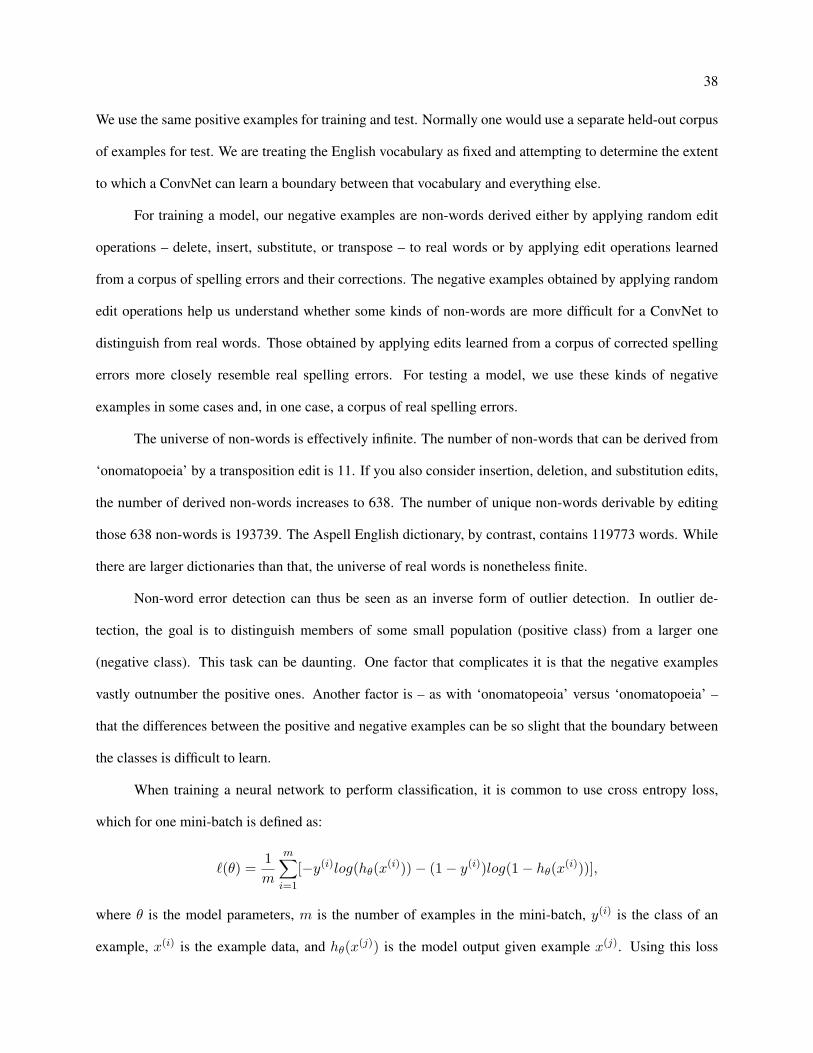
38

We use the same positive examples for training and test. Normally one would use a separate held-out corpus

of examples for test. We are treating the English vocabulary as fixed and attempting to determine the extent

to which a ConvNet can learn a boundary between that vocabulary and everything else.

For training a model, our negative examples are non-words derived either by applying random edit

operations – delete, insert, substitute, or transpose – to real words or by applying edit operations learned

from a corpus of spelling errors and their corrections. The negative examples obtained by applying random

edit operations help us understand whether some kinds of non-words are more difficult for a ConvNet to

distinguish from real words. Those obtained by applying edits learned from a corpus of corrected spelling

errors more closely resemble real spelling errors. For testing a model, we use these kinds of negative

examples in some cases and, in one case, a corpus of real spelling errors.

The universe of non-words is effectively infinite. The number of non-words that can be derived from

‘onomatopoeia’ by a transposition edit is 11. If you also consider insertion, deletion, and substitution edits,

the number of derived non-words increases to 638. The number of unique non-words derivable by editing

those 638 non-words is 193739. The Aspell English dictionary, by contrast, contains 119773 words. While

there are larger dictionaries than that, the universe of real words is nonetheless finite.

Non-word error detection can thus be seen as an inverse form of outlier detection. In outlier de-

tection, the goal is to distinguish members of some small population (positive class) from a larger one

(negative class). This task can be daunting. One factor that complicates it is that the negative examples

vastly outnumber the positive ones. Another factor is – as with ‘onomatopeoia’ versus ‘onomatopoeia’ –

that the differences between the positive and negative examples can be so slight that the boundary between

the classes is difficult to learn.

When training a neural network to perform classification, it is common to use cross entropy loss,

which for one mini-batch is defined as:

ℓ(θ) = 1m

m∑i=1

[−y(i)log(hθ(x(i))) − (1 − y(i))log(1 − hθ(x(i)))],

where θ is the model parameters, m is the number of examples in the mini-batch, y(i) is the class of an

example, x(i) is the example data, and hθ(x(j)) is the model output given example x(j). Using this loss

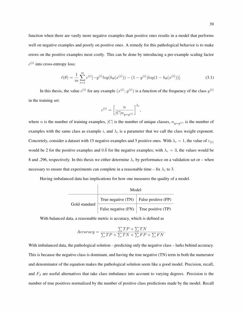
39

function when there are vastly more negative examples than positive ones results in a model that performs

well on negative examples and poorly on positive ones. A remedy for this pathological behavior is to make

errors on the positive examples most costly. This can be done by introducing a per-example scaling factor

c(i) into cross-entropy loss:

ℓ(θ) = 1m

m∑i=1

c(i)[−y(i)log(hθ(x(i))) − (1 − y(i))log(1 − hθ(x(i)))]. (3.1)

In this thesis, the value c(i) for any example (x(i), y(i)) is a function of the frequency of the class y(i)

in the training set:

c(i) =[

n

|C|ny=y(i)

]λc

,

where n is the number of training examples, |C| is the number of unique classes, ny=y(i) is the number of

examples with the same class as example i, and λc is a parameter that we call the class weight exponent.

Concretely, consider a dataset with 15 negative examples and 5 positive ones. With λc = 1, the value of c(i)

would be 2 for the positive examples and 0.6̄ for the negative examples; with λc = 3, the values would be

8 and .296, respectively. In this thesis we either determine λc by performance on a validation set or – when

necessary to ensure that experiments can complete in a reasonable time – fix λc to 3.

Having imbalanced data has implications for how one measures the quality of a model.

Model

Gold standardTrue negative (TN) False positive (FP)

False negative (FN) True positive (TP)

With balanced data, a reasonable metric is accuracy, which is defined as

Accuracy =∑

TP +∑

TN∑TP +

∑TN +

∑FP +

∑FN

.

With imbalanced data, the pathological solution – predicting only the negative class – lurks behind accuracy.

This is because the negative class is dominant, and having the true negative (TN) term in both the numerator

and denominator of the equation makes the pathological solution seem like a good model. Precision, recall,

and Fβ are useful alternatives that take class imbalance into account to varying degrees. Precision is the

number of true positives normalized by the number of positive class predictions made by the model. Recall

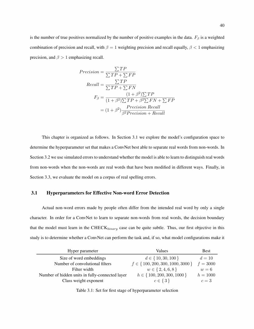
40

is the number of true positives normalized by the number of positive examples in the data. Fβ is a weighted

combination of precision and recall, with β = 1 weighting precision and recall equally, β < 1 emphasizing

precision, and β > 1 emphasizing recall.

Precision =∑

TP∑TP +

∑FP

Recall =∑

TP∑TP +

∑FN

Fβ = (1 + β2)∑

TP

(1 + β2)∑

TP + β2∑FN +

∑FP

= (1 + β2) Precision Recall

β2Precision + Recall

This chapter is organized as follows. In Section 3.1 we explore the model’s configuration space to

determine the hyperparameter set that makes a ConvNet best able to separate real words from non-words. In

Section 3.2 we use simulated errors to understand whether the model is able to learn to distinguish real words

from non-words when the non-words are real words that have been modified in different ways. Finally, in

Section 3.3, we evaluate the model on a corpus of real spelling errors.

3.1 Hyperparameters for Effective Non-word Error Detection

Actual non-word errors made by people often differ from the intended real word by only a single

character. In order for a ConvNet to learn to separate non-words from real words, the decision boundary

that the model must learn in the CHECKbinary case can be quite subtle. Thus, our first objective in this

study is to determine whether a ConvNet can perform the task and, if so, what model configurations make it

Hyper parameter Values Best

Size of word embeddings d ∈ { 10, 30, 100 } d = 10Number of convolutional filters f ∈ { 100, 200, 300, 1000, 3000 } f = 3000

Filter width w ∈ { 2, 4, 6, 8 } w = 6Number of hidden units in fully-connected layer h ∈ { 100, 200, 300, 1000 } h = 1000

Class weight exponent c ∈ { 3 } c = 3

Table 3.1: Set for first stage of hyperparameter selection

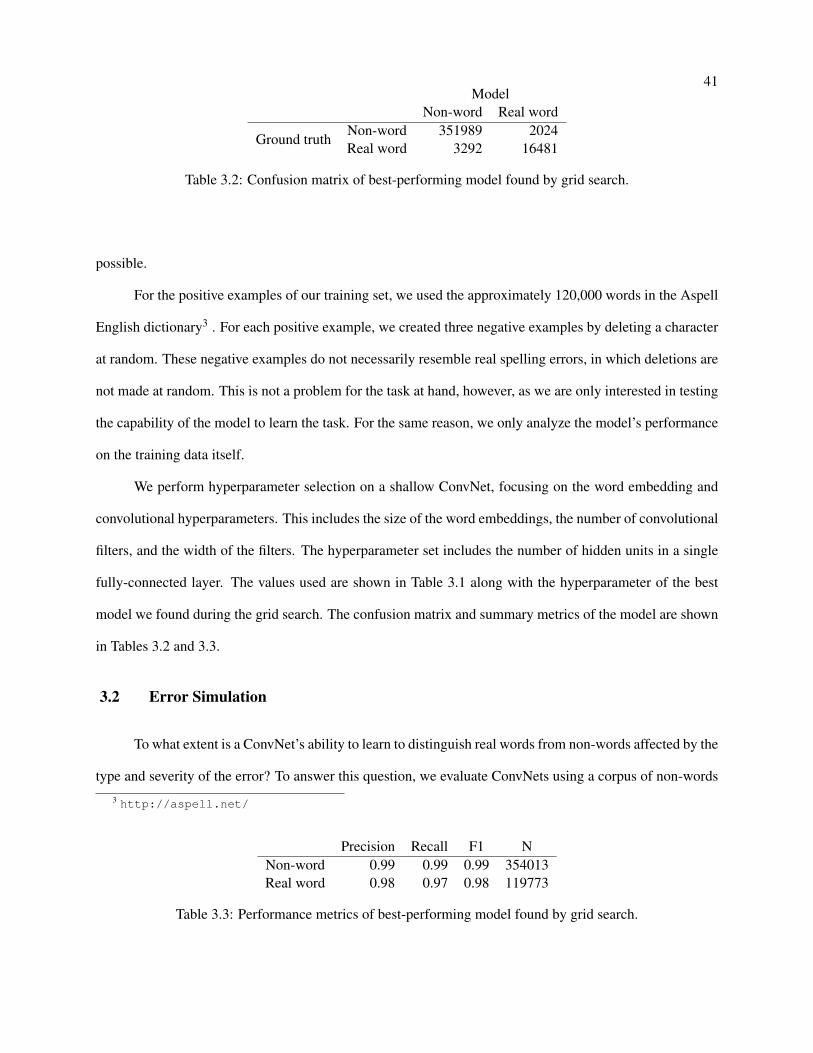
41Model

Non-word Real word

Ground truthNon-word 351989 2024Real word 3292 16481

Table 3.2: Confusion matrix of best-performing model found by grid search.

possible.

For the positive examples of our training set, we used the approximately 120,000 words in the Aspell

English dictionary3 . For each positive example, we created three negative examples by deleting a character

at random. These negative examples do not necessarily resemble real spelling errors, in which deletions are

not made at random. This is not a problem for the task at hand, however, as we are only interested in testing

the capability of the model to learn the task. For the same reason, we only analyze the model’s performance

on the training data itself.

We perform hyperparameter selection on a shallow ConvNet, focusing on the word embedding and

convolutional hyperparameters. This includes the size of the word embeddings, the number of convolutional

filters, and the width of the filters. The hyperparameter set includes the number of hidden units in a single

fully-connected layer. The values used are shown in Table 3.1 along with the hyperparameter of the best

model we found during the grid search. The confusion matrix and summary metrics of the model are shown

in Tables 3.2 and 3.3.

3.2 Error Simulation

To what extent is a ConvNet’s ability to learn to distinguish real words from non-words affected by the

type and severity of the error? To answer this question, we evaluate ConvNets using a corpus of non-words3 http://aspell.net/

Precision Recall F1 NNon-word 0.99 0.99 0.99 354013Real word 0.98 0.97 0.98 119773

Table 3.3: Performance metrics of best-performing model found by grid search.

42

with simulated errors. The error types we consider are insertion, deletion, substitution, and transposition.

The severity of an error is a function of the number of times a given operation has been performed. ‘Trgey’,

for instance, is the result of applying the deletion operation twice to ‘tragedy’.

The confusion matrices for models trained using these artificial negative examples are shown in Table

3.4. The confusion matrices suggest that non-words created with random transpose and insert operations

are easier for the ConvNet to distinguish from real words, and those created with substitutions and deletions

are more difficult. Further understanding of the effects of using different kinds of artificial non-words can

be obtained by a more detailed analysis of these models’ predictions. With that goal in mind, we crafted

a confusion matrix that allows one to inspect a model’s most and least confident predictions. The most

confident predictions are those with high probability for a given class. The least confident ones are those

near the decision boundary between classes. These confusion matrices are supplemented with specific

examples and their corresponding class probabilities, allowing further insight into the model.

Tables 3.5, 3.6, 3.7, and 3.8 show these confusion matrices. A characteristic of all these models is that

when a model predicts a real word with high probability, the word tends to be longer and morphologically

complex, such as ‘impecuniousness’ (Table 3.5), ‘overstimulated’ (Table 3.6), ‘reattaching’ (Table 3.7), and

‘presumptuously’ (Table 3.8). It is clear in Table 3.5 that the ground truth is incorrect – e.g. ‘xiii’ is a word in

the dictionary – and the model has simply learned the regularities in the words of the dictionary so well that

it strongly disagrees with the ground truth. Many other high-probability false positives are orthographically

plausible non-words (e.g. ‘deposites’ in Table 3.7 and ‘stanglers’ in Table 3.8).

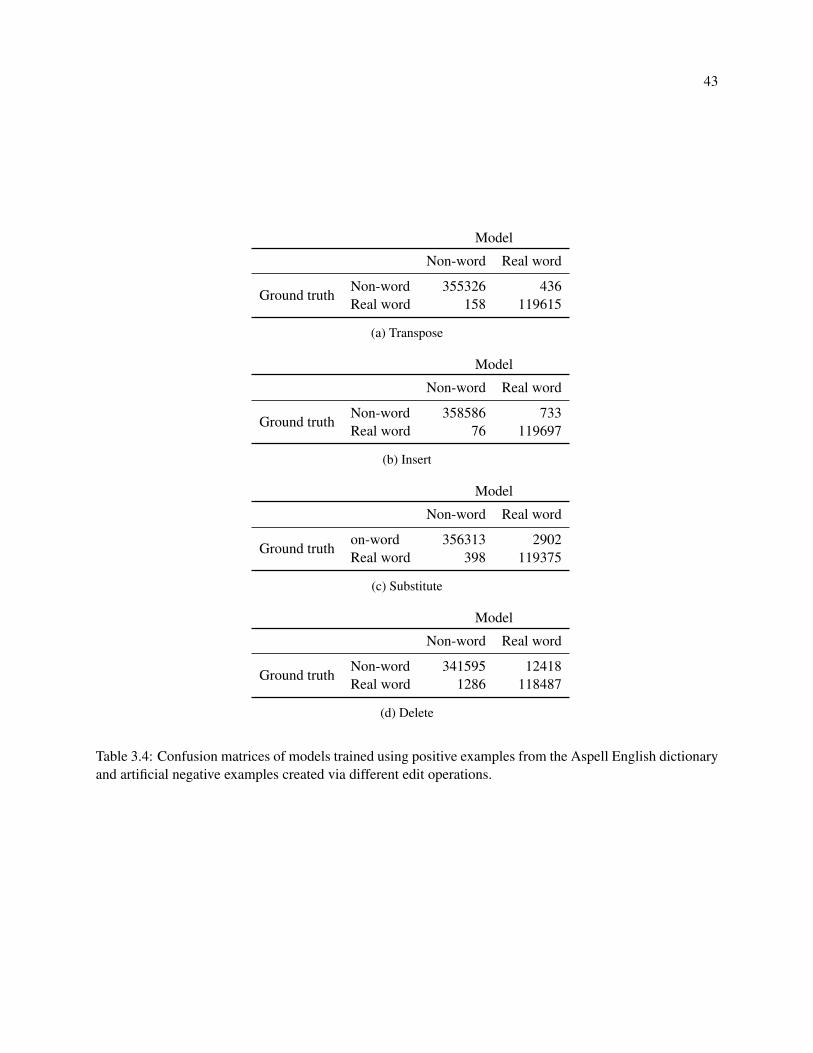
43

Model

Non-word Real word


(a) Transpose

Model

Non-word Real word


(b) Insert

Model

Non-word Real word

Ground truthon-word 356313 2902Real word 398 119375

(c) Substitute

Model

Non-word Real word


(d) Delete

Table 3.4: Confusion matrices of models trained using positive examples from the Aspell English dictionaryand artificial negative examples created via different edit operations.

44

ModelNon-word Real word

Word P(Non-word) Word P(Real word)

Ground truth

Non-word

tbu’s 1.000 xxxi 1.000hardtac’ks 1.000 accoutrements’s 1.000parmiigana 1.000 FORTRANs’ 0.999conujrer 1.000 bodybuidling 0.999synnoymous 1.000 opp 0.999prteense’s 1.000 overacpacity’s 0.997bnater 1.000 sapsmodically 0.997Ber’ts 1.000 Elias’s 0.997everyady 1.000 aah 0.996pruen 1.000 jodhpur’ss 0.995l 0.506 aniums 0.507Judacial 0.506 o 0.507oruses 0.505 orttener 0.506leahs 0.505 GP 0.506grandanuts 0.504 ho 0.506ronate 0.503 AV 0.505JV 0.501 x 0.504PD 0.500 throoughfare’s 0.503centarlist 0.500 Fabereg 0.502CE 0.500 ora 0.502

Real word

PD 0.500 Wodehouse 0.502JV 0.501 x 0.504tsp 0.501 grandiose 0.505dB 0.501 AV 0.505rye’s 0.502 untrue 0.506sere 0.504 ho 0.506dulcet 0.505 GP 0.506l 0.506 o 0.507subset 0.508 fibrosis 0.508lb 0.513 sonsofbitches 0.508Bobbi 0.957 flaccidity 1.000Oliver 0.965 surgeons 1.000honcho 0.967 suspender’s 1.000bobwhites 0.968 musketeer’s 1.000wee 0.982 acidify 1.000Bobbi’s 0.984 washing 1.000Hamlin 0.986 impecuniousness 1.000torches 0.989 afterword’s 1.000weer 0.997 quadruped’s 1.000porches 1.000 appearance 1.000

Table 3.5: Confusion matrix of model trained using artificial negative examples created via a single trans-pose.

45



Ground truth

Non-word

clatrtered 1.000 demorialize 1.000czentres 1.000 Cj’s 1.000Ritqz’s 1.000 sukiyakii’s 0.999xdozes 1.000 deploorable 0.999pwittance 1.000 exjection 0.998feldspaer 1.000 uncorrelanted 0.997purchazser 1.000 Zc’s 0.997hperoics 1.000 beridgework’s 0.997progrzessing 1.000 sv 0.996leafievr 1.000 Cfs 0.996Tic’s 0.505 whorse 0.504keyoed 0.505 rxeefs 0.504Foinn’s 0.504 czaryism 0.504Cague 0.504 Czechts 0.504petulantily 0.504 unnixism 0.504entpirety 0.502 genores 0.503actfresses 0.501 Dorns 0.503bygoney’s 0.501 sedoating 0.502colourfant 0.501 frizzsed 0.501Cheetois 0.500 scalep’s 0.501

Real word

tonguing 0.508 ticking’s 0.501Jamaican’s 0.515 serviceman’s 0.505austere 0.517 abattoir 0.507doctrinaires 0.518 tangle’s 0.513Sinkiang’s 0.519 Isfahan 0.517quadrangle’s 0.522 vainglorious 0.526humeral 0.525 rite 0.529manhunt’s 0.530 pallid 0.532iambic’s 0.531 grand’s 0.535northeastern 0.542 d’Estaing 0.540sacerdotal 0.879 shattering 1.000thong’s 0.889 unsubstantial 1.000undecideds 0.919 grouchiest 1.000bilateral 0.921 codifications 1.000trainmen 0.923 effusing 1.000aberrant 0.934 unsupportable 1.000monomaniacal 0.936 snippet 1.000iambics 0.962 overstimulated 1.000moat 0.974 receptor’s 1.000Noxzema 0.998 schlepping 1.000

Table 3.6: Confusion matrix of model trained using artificial negative examples created via a single insertion.

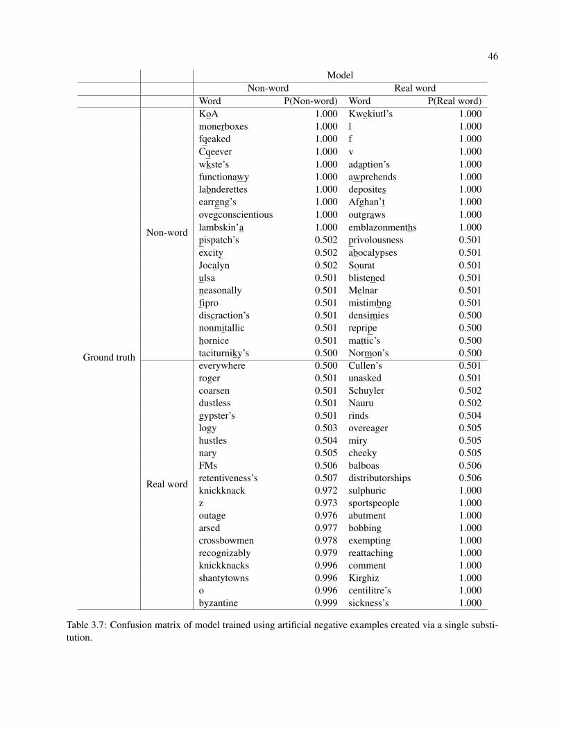
46



Ground truth

Non-word

KoA 1.000 Kwekiutl’s 1.000monerboxes 1.000 l 1.000fqeaked 1.000 f 1.000Cqeever 1.000 v 1.000wkste’s 1.000 adaption’s 1.000functionawy 1.000 awprehends 1.000labnderettes 1.000 deposites 1.000earrgng’s 1.000 Afghan’t 1.000ovegconscientious 1.000 outgraws 1.000lambskin’a 1.000 emblazonmenths 1.000pispatch’s 0.502 privolousness 0.501excity 0.502 abocalypses 0.501Jocalyn 0.502 Sourat 0.501ulsa 0.501 blistened 0.501neasonally 0.501 Melnar 0.501fipro 0.501 mistimbng 0.501discraction’s 0.501 densimies 0.500nonmitallic 0.501 repripe 0.500hornice 0.501 mattic’s 0.500taciturniky’s 0.500 Normon’s 0.500

Real word

everywhere 0.500 Cullen’s 0.501roger 0.501 unasked 0.501coarsen 0.501 Schuyler 0.502dustless 0.501 Nauru 0.502gypster’s 0.501 rinds 0.504logy 0.503 overeager 0.505hustles 0.504 miry 0.505nary 0.505 cheeky 0.505FMs 0.506 balboas 0.506retentiveness’s 0.507 distributorships 0.506knickknack 0.972 sulphuric 1.000z 0.973 sportspeople 1.000outage 0.976 abutment 1.000arsed 0.977 bobbing 1.000crossbowmen 0.978 exempting 1.000recognizably 0.979 reattaching 1.000knickknacks 0.996 comment 1.000shantytowns 0.996 Kirghiz 1.000o 0.996 centilitre’s 1.000byzantine 0.999 sickness’s 1.000

Table 3.7: Confusion matrix of model trained using artificial negative examples created via a single substi-tution.

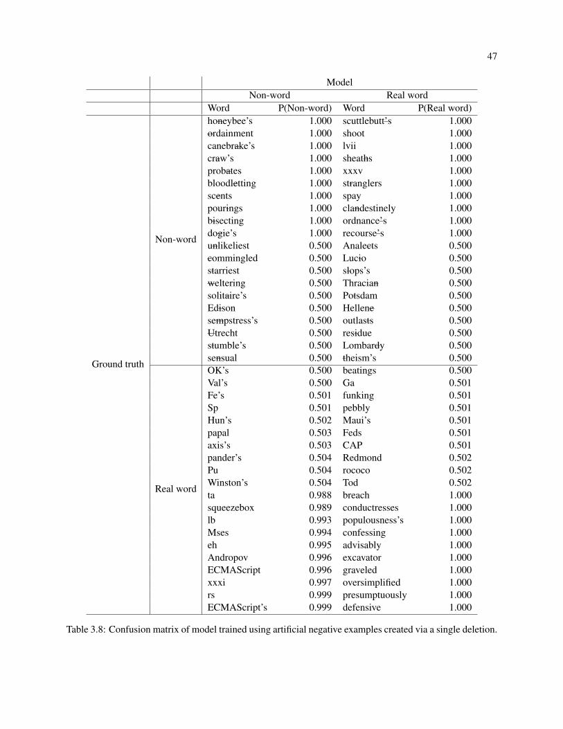
47



Ground truth

Non-word

honeybee’s 1.000 scuttlebutt’s 1.000ordainment 1.000 shoot 1.000canebrake’s 1.000 lvii 1.000craw’s 1.000 sheaths 1.000probates 1.000 xxxv 1.000bloodletting 1.000 stranglers 1.000scents 1.000 spay 1.000pourings 1.000 clandestinely 1.000bisecting 1.000 ordnance’s 1.000dogie’s 1.000 recourse’s 1.000unlikeliest 0.500 Analects 0.500commingled 0.500 Lucio 0.500starriest 0.500 slops’s 0.500weltering 0.500 Thracian 0.500solitaire’s 0.500 Potsdam 0.500Edison 0.500 Hellene 0.500sempstress’s 0.500 outlasts 0.500Utrecht 0.500 residue 0.500stumble’s 0.500 Lombardy 0.500sensual 0.500 theism’s 0.500

Real word

OK’s 0.500 beatings 0.500Val’s 0.500 Ga 0.501Fe’s 0.501 funking 0.501Sp 0.501 pebbly 0.501Hun’s 0.502 Maui’s 0.501papal 0.503 Feds 0.501axis’s 0.503 CAP 0.501pander’s 0.504 Redmond 0.502Pu 0.504 rococo 0.502Winston’s 0.504 Tod 0.502ta 0.988 breach 1.000squeezebox 0.989 conductresses 1.000lb 0.993 populousness’s 1.000Mses 0.994 confessing 1.000eh 0.995 advisably 1.000Andropov 0.996 excavator 1.000ECMAScript 0.996 graveled 1.000xxxi 0.997 oversimplified 1.000rs 0.999 presumptuously 1.000ECMAScript’s 0.999 defensive 1.000

Table 3.8: Confusion matrix of model trained using artificial negative examples created via a single deletion.

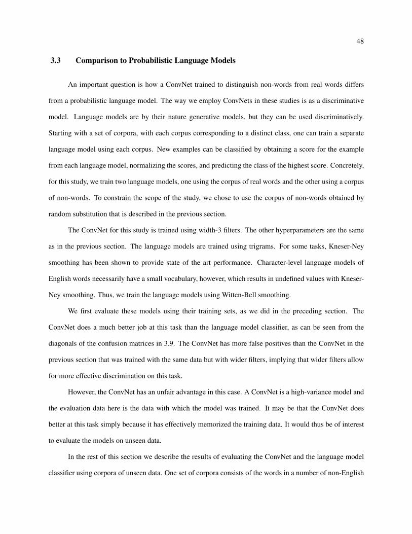
48

3.3 Comparison to Probabilistic Language Models

An important question is how a ConvNet trained to distinguish non-words from real words differs

from a probabilistic language model. The way we employ ConvNets in these studies is as a discriminative

model. Language models are by their nature generative models, but they can be used discriminatively.

Starting with a set of corpora, with each corpus corresponding to a distinct class, one can train a separate

language model using each corpus. New examples can be classified by obtaining a score for the example

from each language model, normalizing the scores, and predicting the class of the highest score. Concretely,

for this study, we train two language models, one using the corpus of real words and the other using a corpus

of non-words. To constrain the scope of the study, we chose to use the corpus of non-words obtained by

random substitution that is described in the previous section.

The ConvNet for this study is trained using width-3 filters. The other hyperparameters are the same

as in the previous section. The language models are trained using trigrams. For some tasks, Kneser-Ney

smoothing has been shown to provide state of the art performance. Character-level language models of

English words necessarily have a small vocabulary, however, which results in undefined values with Kneser-

Ney smoothing. Thus, we train the language models using Witten-Bell smoothing.

We first evaluate these models using their training sets, as we did in the preceding section. The

ConvNet does a much better job at this task than the language model classifier, as can be seen from the

diagonals of the confusion matrices in 3.9. The ConvNet has more false positives than the ConvNet in the

previous section that was trained with the same data but with wider filters, implying that wider filters allow

for more effective discrimination on this task.

However, the ConvNet has an unfair advantage in this case. A ConvNet is a high-variance model and

the evaluation data here is the data with which the model was trained. It may be that the ConvNet does

better at this task simply because it has effectively memorized the training data. It would thus be of interest

to evaluate the models on unseen data.

In the rest of this section we describe the results of evaluating the ConvNet and the language model

classifier using corpora of unseen data. One set of corpora consists of the words in a number of non-English

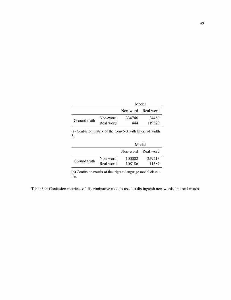
49

Model

Non-word Real word


(a) Confusion matrix of the ConvNet with filters of width3.

Model

Non-word Real word


(b) Confusion matrix of the trigram language model classi-fier.

Table 3.9: Confusion matrices of discriminative models used to distinguish non-words and real words.

50

Aspell dictionaries. The other set consists of 1473 names of companies and brands from Asia, Europe, and

South and North America4 .

The corpora of non-English Aspell dictionaries were obtained by running the command aspell -d

LANG dump master | aspell -l LANG expand, where LANG is the identifier of the language

(e.g. "de" for German"). For most languages, this produced a file with one word per line. For some, such as

Italian, a line contained many variations of a word. To keep processing simple, we kept only the first word

of a line.

Since the ConvNet and language models were trained using only the ASCII character set, we dis-

carded words from these non-English corpora containing non-ASCII characters. Training and evaluating

using only ASCII ensured that the ConvNet and language model classifier would not be biased. We also dis-

carded words that were longer than 25 characters, which is the longest word in the Aspell English dictionary,

and words that appear in the English dictionary. After the preprocessing step, predictions for each word in

each corpus were obtained from the ConvNet and language model classifier. Since none of the words in the

non-English corpora are in the English dictionary, we assigned them a target of 0 (the non-word class) and

computed accuracy as the fraction of a language’s words that a model predicted were not English words.

The results are shown in Table 3.10. The ConvNet is superior to the language model classifier on all

languages. It outperforms the language model classifier by far on all but the Romance languages and Ger-

man, because on those languages the ConvNet performance decreases and the language model performance

increases somewhat. The probability that a word is English according to a model is shown in Table 3.11.

The words in the table were sampled randomly from each language’s vocabulary. Because the accuracy of

the ConvNet is on average higher than the accuracy of the language model, the sampled words tend to be

given a low probability of being English by the ConvNet. A few exceptions exist, such the Italian “Ilena”,

which the ConvNet predicts to be an English word with probability 1.0; this may be because the quite similar

proper names “Irene” and “Elena” are in the English dictionary. Another non-English word that the ConvNet

assigns a high probability is the French “carre” (square in English). The words in the English dictionary

with edit distance 1 from “carre” are “carry”, “carrel”, “care”, “carve”, “barre”, “cadre”, and “carer”. A4 http://www.namedevelopment.com/brand-names.html

51

thorough investigation of why the ConvNet predicts a fraction of the non-English words to be real English

words is beyond the scope of this study, but would be of great interest.

Further evidence of the profound difference between the ConvNet and trigram language model deci-

sion boundaries can be seen in Figure 3.1, which shows the probabilities that a word is English according

to each model. Almost all of the probability mass of the ConvNet is at the extremes, whereas that of the

trigram language model looks very much like a left-skew normal distribution.

Finally, we evaluated the ConvNet and language model classifier on the corpus of 1473 brand and

company names from four continents. The distribution of probabilities for this corpus is shown in Figure

3.2. It is surprising that the ConvNet sees many brand and company names from continents where English

is not the dominant language as being quite English-like. This may reflect the prominence of English as a

language of commerce or, put another way, the emergence of a morphology of branding that is informed by

the prominence of English.

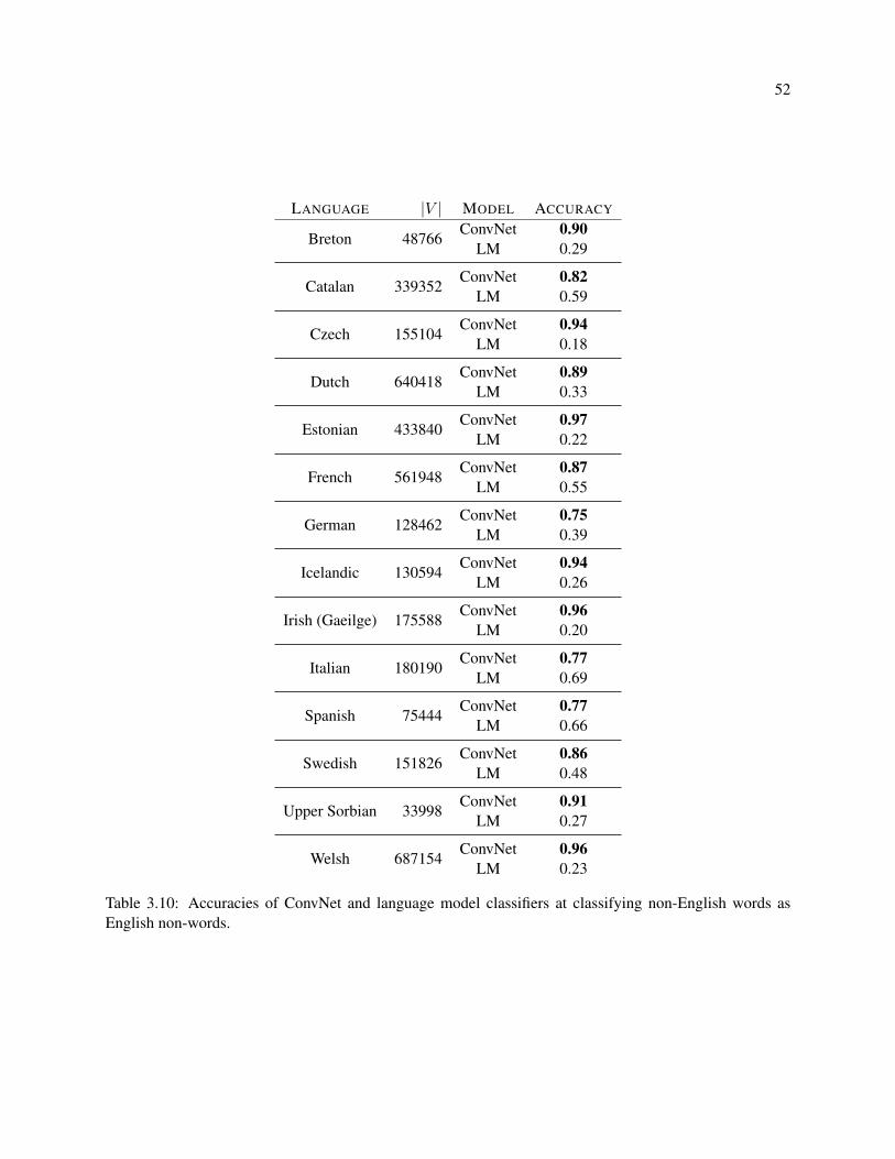
52

LANGUAGE |V | MODEL ACCURACY

Breton 48766ConvNet 0.90

LM 0.29

Catalan 339352ConvNet 0.82

LM 0.59

Czech 155104ConvNet 0.94

LM 0.18

Dutch 640418ConvNet 0.89

LM 0.33

Estonian 433840ConvNet 0.97

LM 0.22

French 561948ConvNet 0.87

LM 0.55

German 128462ConvNet 0.75

LM 0.39

Icelandic 130594ConvNet 0.94

LM 0.26

Irish (Gaeilge) 175588ConvNet 0.96

LM 0.20

Italian 180190ConvNet 0.77

LM 0.69

Spanish 75444ConvNet 0.77

LM 0.66

Swedish 151826ConvNet 0.86

LM 0.48

Upper Sorbian 33998ConvNet 0.91

LM 0.27

Welsh 687154ConvNet 0.96

LM 0.23

Table 3.10: Accuracies of ConvNet and language model classifiers at classifying non-English words asEnglish non-words.

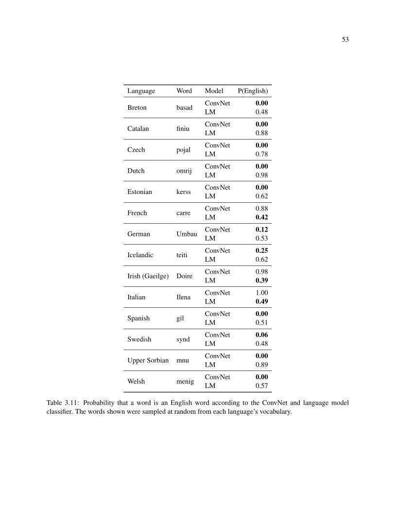
53

Language Word Model P(English)

Breton basadConvNet 0.00LM 0.48

Catalan finiuConvNet 0.00LM 0.88

Czech pojalConvNet 0.00LM 0.78

Dutch omrijConvNet 0.00LM 0.98

Estonian kerssConvNet 0.00LM 0.62

French carreConvNet 0.88LM 0.42

German UmbauConvNet 0.12LM 0.53

Icelandic teitiConvNet 0.25LM 0.62

Irish (Gaeilge) DoireConvNet 0.98LM 0.39

Italian IlenaConvNet 1.00LM 0.49

Spanish gilConvNet 0.00LM 0.51

Swedish syndConvNet 0.06LM 0.48

Upper Sorbian mnuConvNet 0.00LM 0.89

Welsh menigConvNet 0.00LM 0.57

Table 3.11: Probability that a word is an English word according to the ConvNet and language modelclassifier. The words shown were sampled at random from each language’s vocabulary.

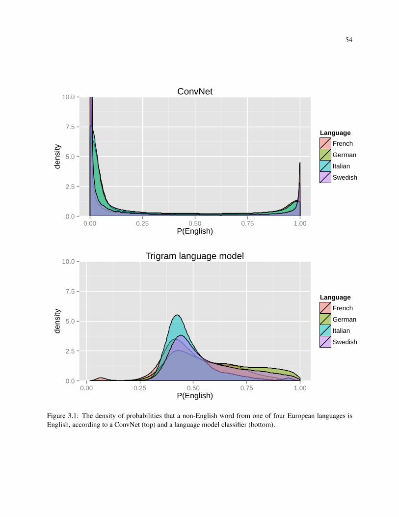
54

0.0

2.5

5.0

7.5

10.0

0.00 0.25 0.50 0.75 1.00P(English)

dens

ity

Language

French

German

Italian

Swedish

ConvNet

0.0

2.5

5.0

7.5

10.0

0.00 0.25 0.50 0.75 1.00P(English)

dens

ity

Language

French

German

Italian

Swedish

Trigram language model

Figure 3.1: The density of probabilities that a non-English word from one of four European languages isEnglish, according to a ConvNet (top) and a language model classifier (bottom).

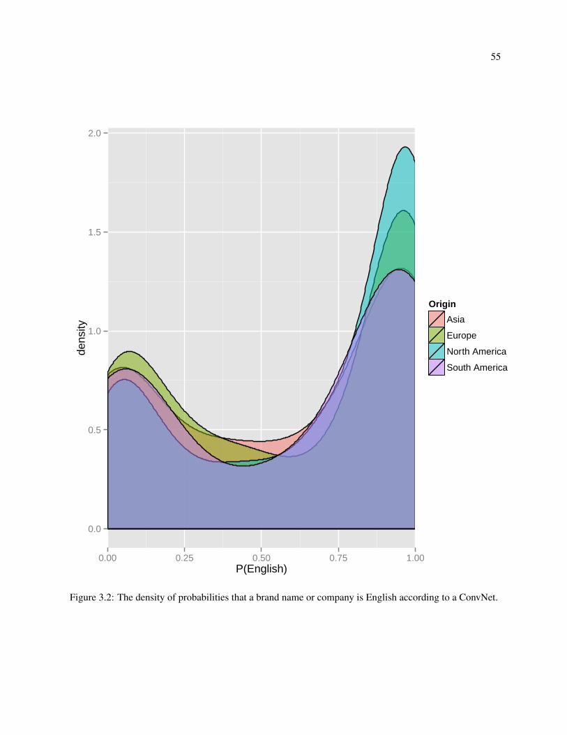
55

0.0

0.5

1.0

1.5

2.0

0.00 0.25 0.50 0.75 1.00P(English)

dens

ity

Origin

Asia

Europe

North America

South America

Figure 3.2: The density of probabilities that a brand name or company is English according to a ConvNet.

56

3.4 Conclusion

In this chapter we investigated the potential of ConvNets as a “soft” dictionary. Specifically, we

trained ConvNets that implement the CHECKbinary interface and found that they can learn to distinguish

English non-words from English real words quite effectively. We also compared a ConvNet to a language

model classifier and found it to be much more robust both at distinguishing English non-words from real

words but also at distinguishing non-English real words from English real words. This suggests that the

boundary that the ConvNet learns around the English vocabulary is quite strong. An evaluation of the

ConvNet on out-of-vocabulary brand and company names from four continents suggests, however, that the

boundary between real English words and all other words is porous and does permit admission of new words.

The stark difference in performance between ConvNets and probabilistic language models shown in

this study supports the hypothesis that ConvNets are capable of achieving greater generalization with smaller

data sets. In this study, ConvNets and language models were trained with identical data, and the ConvNet

performed significantly better. This result is corroborated, although under different experimental conditions,

in the study in Chapter 5, which shows that a ConvNet trained with less data can significantly outperform a

language model trained with vastly more data.

Chapter 4

Study 2: Isolated Non-word Error Correction

We observed in the previous chapter that ConvNets are able to distinguish non-words from real words.

This suggests that they may be able to learn to map non-word errors to their real word corrections. In this

Chapter we move beyond the detection of non-words into correcting them and explore how to perform

isolated non-word error correction effectively using ConvNets. We consider two scenarios: (1) an exter-

nal RETRIEVE component of a spelling error system provides a list of candidates to a ConvNet, which

functions as the system’s RANK component; and (2) a ConvNet functions as both the RETRIEVE and

RANK components. We refer to the former model as the binary model, as it effectively performs binary

classification of pairs of examples, and to the latter model as the multiclass model. We argue that the

distance-based implementations of RANK components suffer from being too simple and rigid and show

that the more complex and flexible behavior of a ConvNet offers superior performance and more intuitive

results. The experiments in this chapter continue our comparison of ConvNets and probabilistic language

models. Specifically, the binary model is evaluated against another model that is trained with – among other

features – the unigram probability of the candidate word, thus giving it access to contextual information that

the purely isolated correction models lack.

Section 4.1 begins this Chapter with a discussion of the corpora we use for training and evaluation.

In Section 4.2 we discuss traditional ways of implementing the RANK component of a spelling error sys-

tem. Section 4.3 introduces and evaluates our binary model, and Section 4.4 introduces and evaluates our

multiclass model.

58Corpus Errors Vocabulary Real word errors (%)Aspell 531 450 18 (3)

Birbeck 36133 6136 3750 (10)Holbrook 1771 1199 544 (3)

Wikipedia 2455 1922 37 (2)

Table 4.1: Summaries of the corpora of spelling errors and corrections archived by Prof. Mitton.

4.1 Corpora

In this Chapter we use two kinds of corpora. One consists of real examples of non-word errors and

their corrections; these corpora are available from the web site of Prof. Roger Mitton1 . The other kind of

corpora consist of examples obtained by learning patterns of edits from the Mitton corpora and applying

the edits to real words to generate plausible examples of non-words. This process yields a new corpus of

non-words and corrections that is larger than all of the Mitton corpora combined and that covers the entire

Aspell English dictionary.

4.1.0.1 Mitton Corpora

The number of errors and unique corrections in each of the corpora obtained from Prof. Mitton

are shown in Table 4.1. The table also shows the number and percentage of the errors that are real word

errors. These are important because determining the true correction for such errors requires knowledge of

the context of the real word error. Since in this Chapter we are only considering isolated non-word error

correction, we exclude these errors from our evaluation.

While these corpora are a valuable resource, they are nonetheless quite small, particularly for training

high-variance models such as convolutional networks. These corpora also cover a relatively small fraction

of the Aspell English dictionary. Thus, we only use the Mitton corpora to evaluate our ConvNets, not to

train them.1 http://www.dcs.bbk.ac.uk/~ROGER/corpora.html

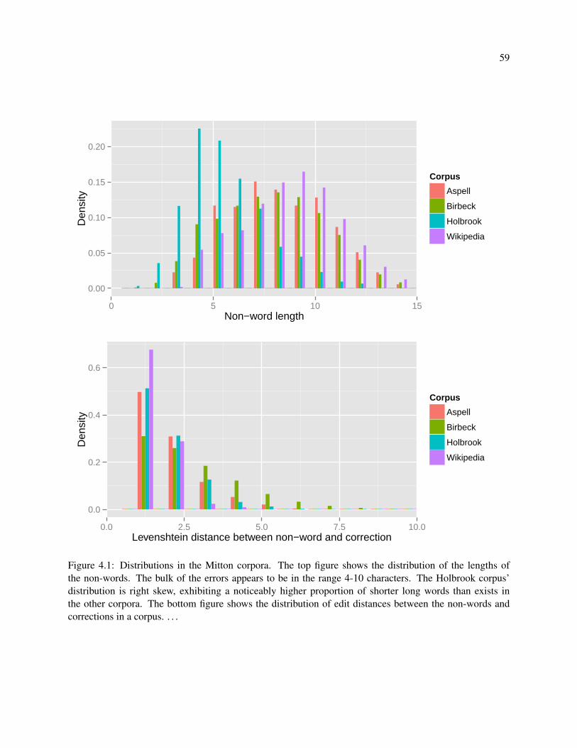
59

0.00

0.05

0.10

0.15

0.20

0 5 10 15Non−word length

Den

sity

Corpus

Aspell

Birbeck

Holbrook

Wikipedia

0.0

0.2

0.4

0.6

0.0 2.5 5.0 7.5 10.0Levenshtein distance between non−word and correction

Den

sity

Corpus

Aspell

Birbeck

Holbrook

Wikipedia

Figure 4.1: Distributions in the Mitton corpora. The top figure shows the distribution of the lengths ofthe non-words. The bulk of the errors appears to be in the range 4-10 characters. The Holbrook corpus’distribution is right skew, exhibiting a noticeably higher proportion of shorter long words than exists inthe other corpora. The bottom figure shows the distribution of edit distances between the non-words andcorrections in a corpus. . . .

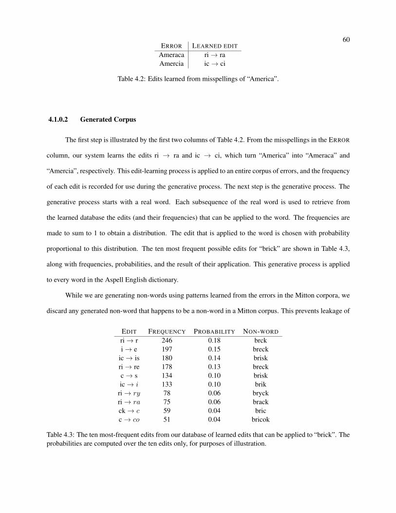
60ERROR LEARNED EDIT

Ameraca ri → raAmercia ic → ci

Table 4.2: Edits learned from misspellings of “America”.

4.1.0.2 Generated Corpus

The first step is illustrated by the first two columns of Table 4.2. From the misspellings in the ERROR

column, our system learns the edits ri → ra and ic → ci, which turn “America” into “Ameraca” and

“Amercia”, respectively. This edit-learning process is applied to an entire corpus of errors, and the frequency

of each edit is recorded for use during the generative process. The next step is the generative process. The

generative process starts with a real word. Each subsequence of the real word is used to retrieve from

the learned database the edits (and their frequencies) that can be applied to the word. The frequencies are

made to sum to 1 to obtain a distribution. The edit that is applied to the word is chosen with probability

proportional to this distribution. The ten most frequent possible edits for “brick” are shown in Table 4.3,

along with frequencies, probabilities, and the result of their application. This generative process is applied

to every word in the Aspell English dictionary.

While we are generating non-words using patterns learned from the errors in the Mitton corpora, we

discard any generated non-word that happens to be a non-word in a Mitton corpus. This prevents leakage of

EDIT FREQUENCY PROBABILITY NON-WORD

ri → r 246 0.18 brcki → e 197 0.15 breck

ic → is 180 0.14 briskri → re 178 0.13 breckc → s 134 0.10 briskic → i 133 0.10 brik

ri → ry 78 0.06 bryckri → ra 75 0.06 brackck → c 59 0.04 bricc → co 51 0.04 bricok

Table 4.3: The ten most-frequent edits from our database of learned edits that can be applied to “brick”. Theprobabilities are computed over the ten edits only, for purposes of illustration.

61

data from the training set to the Mitton corpora.

4.2 Baselines

In this section we introduce the non-ConvNet RETRIEVE and RANK components we use in exper-

iments for this study. The RETRIEVE component described here is used to create candidate lists for the

baseline RANK components described in this section as well as for the binary ConvNet model. The RANK

components are used as baselines against which the binary and multiclass ConvNet models are evaluated.

4.2.1 Near-miss and Aspell RETRIEVE

There are several ways that the RETRIEVE component of a spelling system can be implemented. A

conventional method that probably originated with the ispell UNIX command is a near-miss strategy2

In this procedure, the candidate list is retrieved by applying a set of transformations to the non-word and re-

turning any that are in the dictionary. The transformations include character insertion, deletion, substitution,

transposition, and the insertion of a space or hyphen. The result is a list of candidates with a Damerau-

Levenshtein distance of 1 from the non-word. The procedure can be applied again to obtain candidates with

distance 2. The number of transformations increases supra-linearly with distance, so retrieving candidates

of distance 3 or greater is computationally prohibitive. The use of this method thus effectively precludes the

retrieval of any candidate that is further than distance 2 from the non-word.

Retrieval of more distant candidates is possible using a phonetic matching strategy. Phonetic matching

is a technique for identifying words that sound alike but are spelled differently. At the core of the method

is an algorithm that encodes a word in a way that approximates its phonemes. Once two words have been

encoded in this way, their encodings are compared; if they are identical, the words are said to match. An

example using the Metaphone algorithm may be helpful. Consider “hifin”, a misspelling of “hyphen”.

Its Metaphone encoding is “HFN”. The candidate list retrieved from the Aspell English dictionary using

phonetic matching is shown in Table 4.4. Note that the edit distance of the true correction is greater than2 See this mention of its near-miss strategy in the Aspell documentation: http://aspell.net/man-html/

Aspell-Suggestion-Strategy.html. This strategy is described by Peterson in reference to the PDP-10 spell checker,of which ispell is a descendant [Pet80].

62

is possible using the conventional near-miss strategy. Phonetic matching thus makes it possible to retrieve

the true corrections of errors made by young learners and second language learners, who sometimes use a

“sound it out” technique to spell a word when they are unfamiliar with its morphology.

The RETRIEVE component of the Aspell spelling correction system combines the near-miss and

phonetic matching strategies. It retrieves candidates by applying the near-miss strategy to Metaphone en-

codings. Specifically, a word is retrieved if its Metaphone encoding is within Levenshtein distance 2 of the

Metaphone encoding of the non-word. The phonetic matching strategy and Aspell’s hybrid strategy produce

candidate lists that can be much longer than those produced by the near-miss strategy alone. This can be

seen in Figure 4.2, which shows the distribution of the length of candidate lists produced using near-miss

retrieval or Aspell.

The RETRIEVE component we use in this study consists of two RETRIEVE sub-components: one

that uses the near-miss strategy and another that uses Aspell. We have observed that Aspell’s strategy some-

times fails to include words that a simple implementation of the near-miss strategy includes. By combining

the strategies, we overcome that limitation in the Aspell implementation. Our component obtains a candidate

list for a given non-word from each sub-component and discards duplicate candidates.

4.2.2 Jaro-Winkler RANK

The RANK component of traditional isolated spelling correction systems is often based on some

measure of distance between a non-word and its correction. The quite reasonable assumption behind the use

of such string metrics approaches is that a misspelling will be largely correct except for a few characters. In

his seminal paper on string edit distance, Levenshtein proposed to measure the distance between strings as

the number of insertion, deletion, and substitution operations needed to transform one string into the other

[Lev66]. Damerau-Levenshtein distance is an extension of this that includes transpositions [Dam64a]. Jaro

distance measures similarity as a function of the number of matching proximal characters and the number

of transpositions [Jar89]. Using the insight that spelling errors are less likely at the beginning of a word,

Jaro-Winkler improves Jaro distance by favoring pairs of strings with identical prefixes [Win90].

Better corrections can be achieved by using corpus statistics to obtain a language model with which

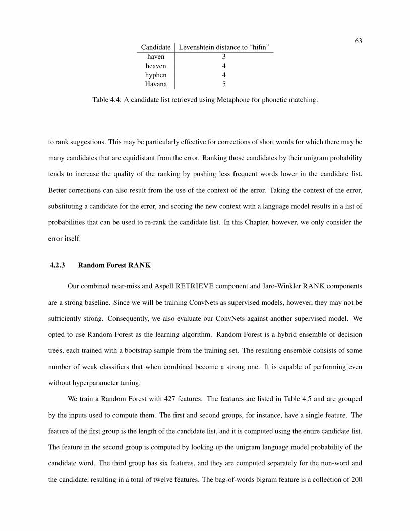
63Candidate Levenshtein distance to “hifin”

haven 3heaven 4hyphen 4Havana 5

Table 4.4: A candidate list retrieved using Metaphone for phonetic matching.

to rank suggestions. This may be particularly effective for corrections of short words for which there may be

many candidates that are equidistant from the error. Ranking those candidates by their unigram probability

tends to increase the quality of the ranking by pushing less frequent words lower in the candidate list.

Better corrections can also result from the use of the context of the error. Taking the context of the error,

substituting a candidate for the error, and scoring the new context with a language model results in a list of

probabilities that can be used to re-rank the candidate list. In this Chapter, however, we only consider the

error itself.

4.2.3 Random Forest RANK

Our combined near-miss and Aspell RETRIEVE component and Jaro-Winkler RANK components

are a strong baseline. Since we will be training ConvNets as supervised models, however, they may not be

sufficiently strong. Consequently, we also evaluate our ConvNets against another supervised model. We

opted to use Random Forest as the learning algorithm. Random Forest is a hybrid ensemble of decision

trees, each trained with a bootstrap sample from the training set. The resulting ensemble consists of some

number of weak classifiers that when combined become a strong one. It is capable of performing even

without hyperparameter tuning.

We train a Random Forest with 427 features. The features are listed in Table 4.5 and are grouped

by the inputs used to compute them. The first and second groups, for instance, have a single feature. The

feature of the first group is the length of the candidate list, and it is computed using the entire candidate list.

The feature in the second group is computed by looking up the unigram language model probability of the

candidate word. The third group has six features, and they are computed separately for the non-word and

the candidate, resulting in a total of twelve features. The bag-of-words bigram feature is a collection of 200

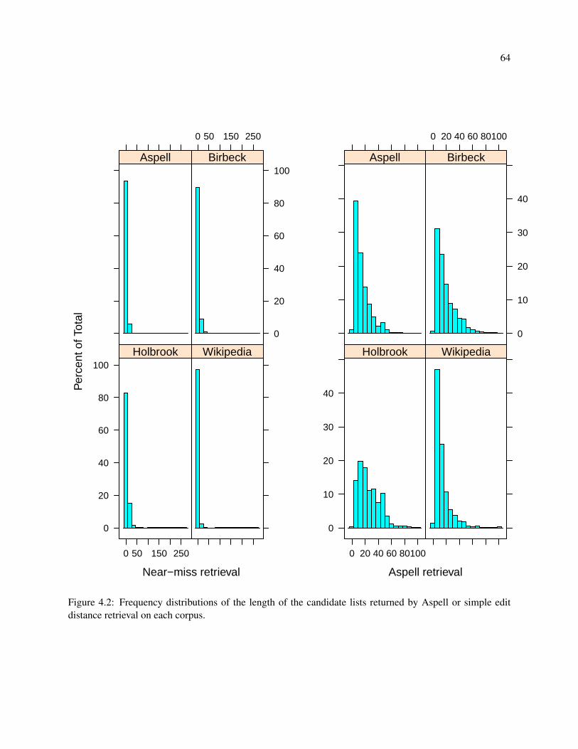
64

Near−miss retrieval

Per

cent

of T

otal

0

20

40

60

80

100

0 50 150 250

Holbrook Wikipedia

Aspell

0 50 150 250

0

20

40

60

80

100Birbeck

Aspell retrieval

0

10

20

30

40

0 20 40 60 80100

Holbrook Wikipedia

Aspell

0 20 40 60 80100

0

10

20

30

40

Birbeck

Figure 4.2: Frequency distributions of the length of the candidate lists returned by Aspell or simple editdistance retrieval on each corpus.

65

features, which provides most of the actual features since each feature in this group is computed for both

the non-word and the candidate.

The fourth group in Table 4.5 is perhaps the most interesting. The group has twenty features, each of

which is the distance between the non-word and candidate using some metric and some representation of the

non-word and candidate. Using multiple metrics and multiple representations of the same inputs provides

the Random Forest a multitude of slightly-varying views of the training examples. This ensemble of views

provides a fine-grained view of the relationship between non-words and candidates.

The Random Forest was trained as follows. Given a non-word, the RETRIEVE component was used

to obtain a candidate list. The features in Table 4.5 were computed for each candidate. The target variable

of each feature vector was set to 0 if the candidate was not the true correction and 1 otherwise. At training

time, the model is trained only to predict the true correction. In a given candidate list, all labels are 0 except

for that of the true correction. The loss of the Random Forest model is scaled according to Equation 3 with

an exponent of 1; consequently, an error on the true correction is the most costly for the model to make.

In a supervised learning setting, training a model with (1) ensemble-of-views inputs such as those

in the fourth group of Table 4.5 and (2) the bag-of-words bigram feature in the third group of Table 4.5

should in principle give the model an opportunity to learn mapping from the (non-word, candidate) inputs

to the candidate that is most likely to be the true correction. This makes the Random Forest RANK a strong

baseline against which to evaluate our ConvNets.

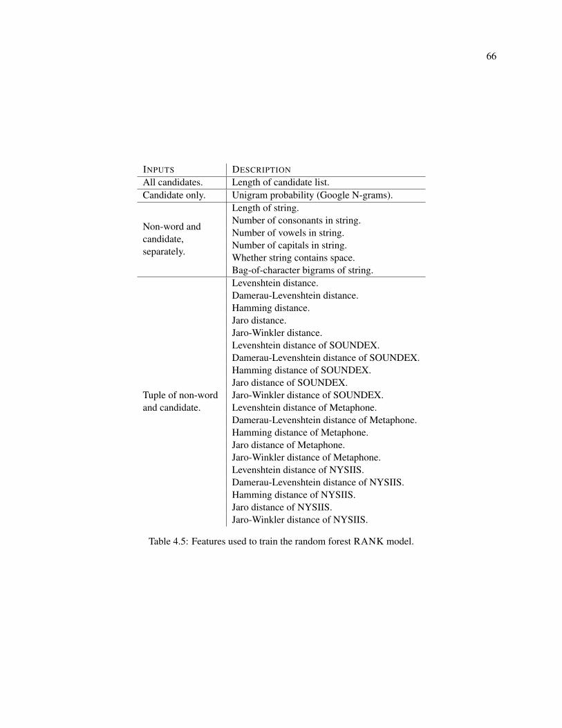
66

INPUTS DESCRIPTION

All candidates. Length of candidate list.Candidate only. Unigram probability (Google N-grams).

Non-word andcandidate,separately.

Length of string.Number of consonants in string.Number of vowels in string.Number of capitals in string.Whether string contains space.Bag-of-character bigrams of string.

Tuple of non-wordand candidate.

Levenshtein distance.Damerau-Levenshtein distance.Hamming distance.Jaro distance.Jaro-Winkler distance.Levenshtein distance of SOUNDEX.Damerau-Levenshtein distance of SOUNDEX.Hamming distance of SOUNDEX.Jaro distance of SOUNDEX.Jaro-Winkler distance of SOUNDEX.Levenshtein distance of Metaphone.Damerau-Levenshtein distance of Metaphone.Hamming distance of Metaphone.Jaro distance of Metaphone.Jaro-Winkler distance of Metaphone.Levenshtein distance of NYSIIS.Damerau-Levenshtein distance of NYSIIS.Hamming distance of NYSIIS.Jaro distance of NYSIIS.Jaro-Winkler distance of NYSIIS.

Table 4.5: Features used to train the random forest RANK model.

67

4.3 Binary ConvNet Model

4.3.1 Architecture

The binary classification ConvNet we present and evaluate in this section implements a spelling sys-

tem’s RANK component and thus relies on an external RETRIEVE component. The baseline dictionary

described in the previous section serves as the RETRIEVE component. The model takes pairs of examples

as input. The pairs consist of the non-word to be corrected and a candidate real word from the dictionary.

The model is trained to predict whether the candidate is the true correction.

A training mini-batch comprises all of the baseline dictionary’s suggestions for a non-word. An

example is shown in the following table for the spelling error “hifin”. In this mini-batch, the model is

presented the pairs (hifin, haven), (hifin, hyphen), (hifin, heaven), and (hifin, Havana), in that order. This

order is the same as the rank of the dictionary’s suggestions; since the ConvNet is stateless, presenting the

examples in this way cannot induce the model simply to memorize the order of the inputs.

Non-word Candidate Target Jaro-Winkler

^hifin$ ^haven$ 0 .60

^hifin$ ^hyphen$ 1 .58

^hifin$ ^heaven$ 0 .58

^hifin$ ^Havana$ 0 .46

Note that each string begins with a caret and ends with a dollar sign. These are conventional regular

expression symbols that denote the beginning and end of a string, respectively. Here they are used as markers

that allow a ConvNet’s filters to orient themselves when processing an input. The character embedding

matrix was comprised of 255 embeddings. Characters were mapped into the embedding matrix by taking

their ASCII codes.

The architecture of the model is shown in Figure 4.3. The character vectors of the non-word (red)

and the candidate word (green) are retrieved from the same character embedding layer (not shown, for

compactness) to construct an embedding matrix for each string. Noise sampled from a normal distribution

with some small variance σ is added to the non-word embedding matrix. The embedding matrices are then

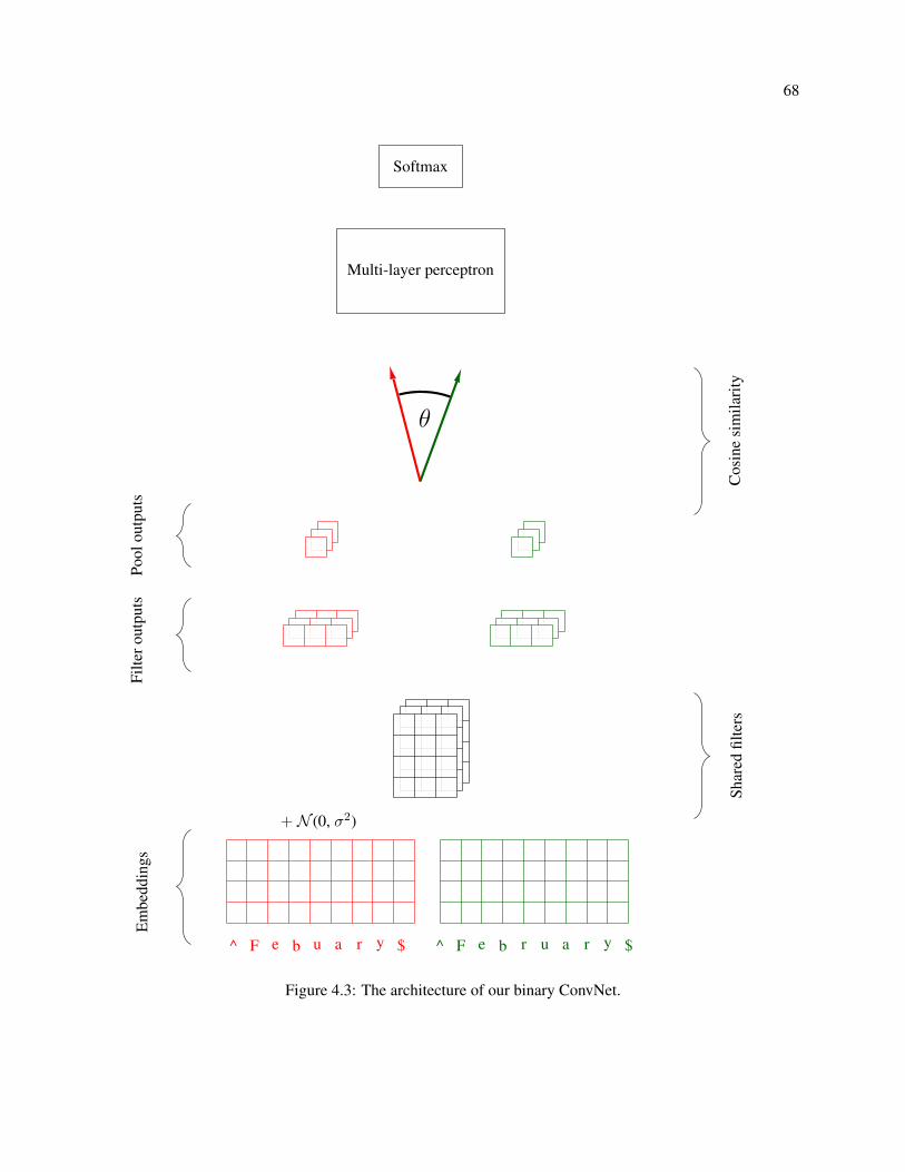
68

+ N (0, σ2)

^ F e b u a r y $ ^ F e b r u a r y $

θ

Multi-layer perceptron

Softmax

Em

bedd

ings

Filte

rout

puts

Pool

outp

uts

Shar

edfil

ters

Cos

ine

sim

ilari

ty

Figure 4.3: The architecture of our binary ConvNet.

69

separately processed by a layer of convolutional filters. That yields a variable-width number of outputs for

each filter for both the non-word and the candidate word. The pooling operation reduces the convolutional

outputs to a fixed-width vector for each string. A key element of the network is the next layer, which

computes the cosine similarity of the fixed-width vectors. The scalar output of cosine similarity is then input

to a multilayer perceptron and finally to a softmax output layer. Because the embedding and convolutional

layers are used to process both the non-word and the candidate word, this network resembles a Siamese

network. A Siamese network takes two inputs and processes them in the same way using one or more

shared layers that share weights. What distinguishes this network from a Siamese network is that noise is

added to the non-word but not the candidate word embedding matrix. Adding noise only to the non-word is

a model-specific way to simulate having more non-words than we actually do.

4.3.2 Evaluation

We trained the binary model using 90% of a corpus of generated errors containing 3,508,455 non-

words. The number of non-words of each length in the corpus is shown in Table 4.6. The remaining 10% of

non-words in the corpus was split in half for validation and test (175,422 for each).

The dimensionality of the embedding matrix was set to 10, the number of filters was set to 2,000,

and the filter width was set to 6. The multilayer perceptron was configured with three layers with 100

hidden units each. We found that having one or more layers in the multilayer perceptron after the cosine

similarity operation made the network more stable during training. Without it, the performance could vary a

great deal from epoch to epoch. The non-linearity used was the rectified linear (ReLU) function, defined as

max(x, 0). Weight updates were done by the Adam optimization algorithm [KA15]. Using early stopping,

the model was trained for 78 epochs.

Figure 4.4 shows the accuracy of the model at rank k on the test set of generated non-words. It is

clear that the shorter a non-word, the more difficult it is to correct. If you assume that non-words tend to

be of approximately the same length as their intended word, and that the fraction of incorrect characters in

a non-word tends to grow sublinearly with length, then a longer non-word is easier to correct than a shorter

one, because the longer one has more correct characters. The ConvNet’s performance on these data exceeds

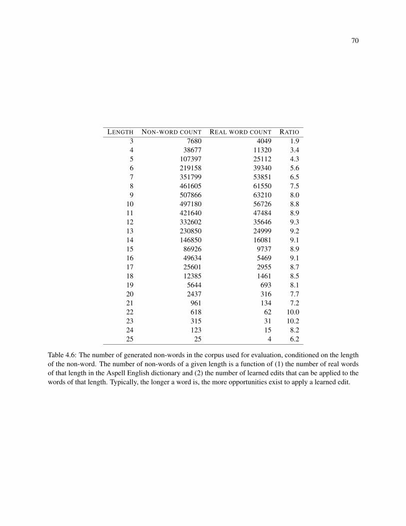
70

LENGTH NON-WORD COUNT REAL WORD COUNT RATIO

3 7680 4049 1.94 38677 11320 3.45 107397 25112 4.36 219158 39340 5.67 351799 53851 6.58 461605 61550 7.59 507866 63210 8.0

10 497180 56726 8.811 421640 47484 8.912 332602 35646 9.313 230850 24999 9.214 146850 16081 9.115 86926 9737 8.916 49634 5469 9.117 25601 2955 8.718 12385 1461 8.519 5644 693 8.120 2437 316 7.721 961 134 7.222 618 62 10.023 315 31 10.224 123 15 8.225 25 4 6.2

Table 4.6: The number of generated non-words in the corpus used for evaluation, conditioned on the lengthof the non-word. The number of non-words of a given length is a function of (1) the number of real wordsof that length in the Aspell English dictionary and (2) the number of learned edits that can be applied to thewords of that length. Typically, the longer a word is, the more opportunities exist to apply a learned edit.

71

that of the Jaro-Winkler baseline for all but the shortest words. The difference in accuracy-at-k between

them is shown in Figure 4.5.

We then retrieved candidate lists for each of the non-words in the four Mitton corpora (Aspell, Bir-

beck, Holbrook, and Wikipedia). We used Jaro-Winkler distance as one baseline RANK component. We

used the Random Forest RANK model as the other. To rank the candidate lists for a given Mitton corpus,

we trained the Random Forest on the other three corpora, removing from the training corpora any non-words

that were also in the test corpus. Finally, we used the ConvNet binary model trained using the generated

non-words to rank the candidate lists for each corpus. The accuracy at rank K of each approach is shown

Table 4.7. The Random Forest model is a very strong baseline and outperforms the other approaches most

of the time. The ConvNet tends to outperform Jaro-Winkler distance RANK especially for K < 3, except

for on the Holbrook corpus, the ConvNet does quite poorly.

A comparison of the three approaches broken down by the length of the non-word can be seen in

Figure 4.6. As with the aggregate performance, the Random Forest RANK model generally outperforms

the others, but this detailed view of the results highlights some relateive weaknesses of the Random Forest.

Jaro-Winkler holds up against Random Forest on non-words of length 6 or greater at rank K < 2 and the

ConvNet outperforms the Random Forest on longer non-words staring at K = 2. This is interesting because

it suggests there are aspects of those non-words that the Random Forest is not able to condition itself on.

Overall, these results indicate that a ConvNet is in many cases superior to Jaro-Winkler distance at this

task. More error analysis is necessary to understand the ConvNet’s performance on the Holbrook corpus.

The general and pronounced superiority of the Random Forest model suggests that a good RANK compo-

nent in an isolated non-word error correction system should take advantage of more than just character-level

lexical similarity between a non-word and the candidates.

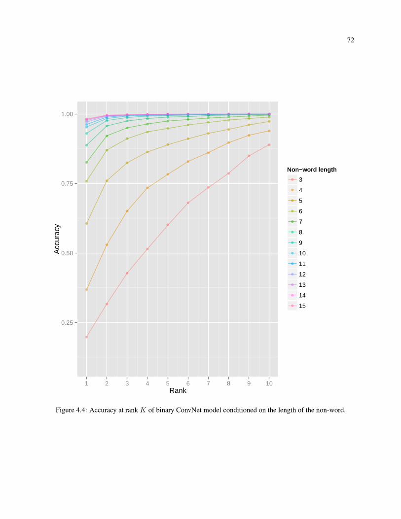
72

0.25

0.50

0.75

1.00

1 2 3 4 5 6 7 8 9 10Rank

Acc

urac

y

Non−word length

3

4

5

6

7

8

9

10

11

12

13

14

15

Figure 4.4: Accuracy at rank K of binary ConvNet model conditioned on the length of the non-word.

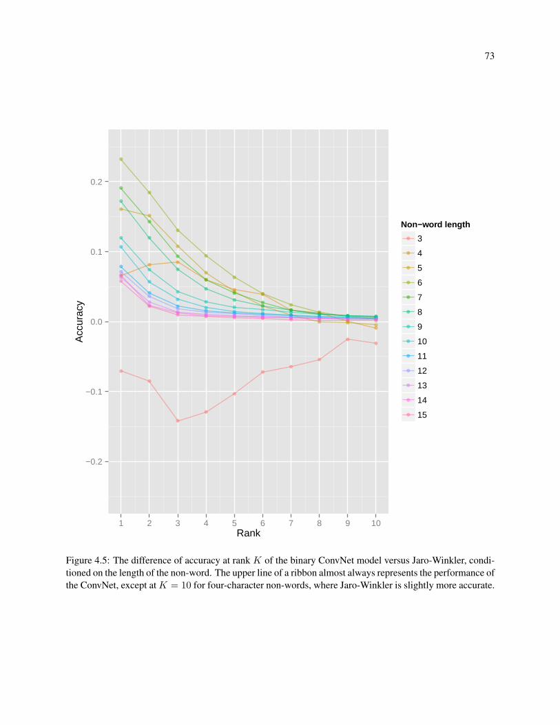
73

−0.2

−0.1

0.0

0.1

0.2

1 2 3 4 5 6 7 8 9 10Rank

Acc

urac

y

Non−word length

3

4

5

6

7

8

9

10

11

12

13

14

15

Figure 4.5: The difference of accuracy at rank K of the binary ConvNet model versus Jaro-Winkler, condi-tioned on the length of the non-word. The upper line of a ribbon almost always represents the performance ofthe ConvNet, except at K = 10 for four-character non-words, where Jaro-Winkler is slightly more accurate.

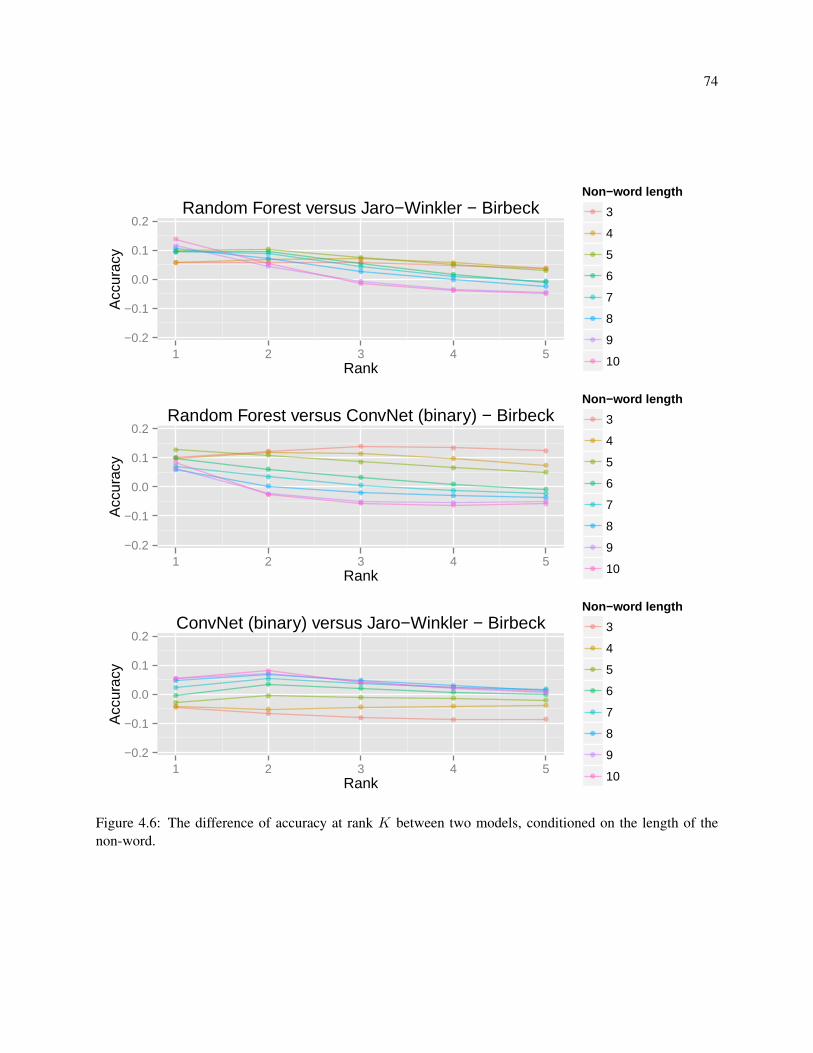
74

−0.2

−0.1

0.0

0.1

0.2

1 2 3 4 5Rank

Acc

urac

y

Non−word length

3

4

5

6

7

8

9

10

Random Forest versus Jaro−Winkler − Birbeck

−0.2

−0.1

0.0

0.1

0.2

1 2 3 4 5Rank

Acc

urac

y

Non−word length

3

4

5

6

7

8

9

10

Random Forest versus ConvNet (binary) − Birbeck

−0.2

−0.1

0.0

0.1

0.2

1 2 3 4 5Rank

Acc

urac

y

Non−word length

3

4

5

6

7

8

9

10

ConvNet (binary) versus Jaro−Winkler − Birbeck

Figure 4.6: The difference of accuracy at rank K between two models, conditioned on the length of thenon-word.

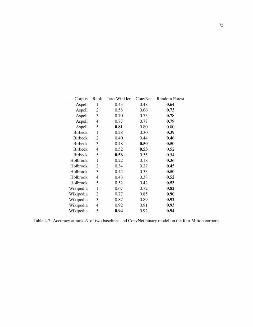
75

Corpus Rank Jaro-Winkler ConvNet Random ForestAspell 1 0.43 0.48 0.64Aspell 2 0.58 0.66 0.73Aspell 3 0.70 0.73 0.78Aspell 4 0.77 0.77 0.79Aspell 5 0.81 0.80 0.80

Birbeck 1 0.28 0.30 0.39Birbeck 2 0.40 0.44 0.46Birbeck 3 0.48 0.50 0.50Birbeck 4 0.52 0.53 0.52Birbeck 5 0.56 0.55 0.54

Holbrook 1 0.22 0.18 0.36Holbrook 2 0.34 0.27 0.45Holbrook 3 0.42 0.33 0.50Holbrook 4 0.48 0.38 0.52Holbrook 5 0.52 0.42 0.53

Wikipedia 1 0.67 0.72 0.82Wikipedia 2 0.77 0.85 0.90Wikipedia 3 0.87 0.89 0.92Wikipedia 4 0.92 0.91 0.93Wikipedia 5 0.94 0.92 0.94

Table 4.7: Accuracy at rank K of two baselines and ConvNet binary model on the four Mitton corpora.

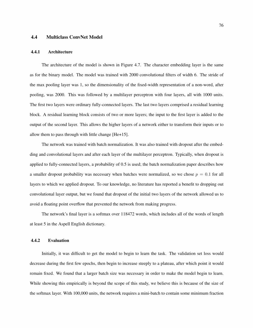
76

4.4 Multiclass ConvNet Model

4.4.1 Architecture

The architecture of the model is shown in Figure 4.7. The character embedding layer is the same

as for the binary model. The model was trained with 2000 convolutional filters of width 6. The stride of

the max pooling layer was 1, so the dimensionality of the fixed-width representation of a non-word, after

pooling, was 2000. This was followed by a multilayer perceptron with four layers, all with 1000 units.

The first two layers were ordinary fully-connected layers. The last two layers comprised a residual learning

block. A residual learning block consists of two or more layers; the input to the first layer is added to the

output of the second layer. This allows the higher layers of a network either to transform their inputs or to

allow them to pass through with little change [He+15].

The network was trained with batch normalization. It was also trained with dropout after the embed-

ding and convolutional layers and after each layer of the multilayer perceptron. Typically, when dropout is

applied to fully-connected layers, a probability of 0.5 is used; the batch normalization paper describes how

a smaller dropout probability was necessary when batches were normalized, so we chose p = 0.1 for all

layers to which we applied dropout. To our knowledge, no literature has reported a benefit to dropping out

convolutional layer output, but we found that dropout of the initial two layers of the network allowed us to

avoid a floating point overflow that prevented the network from making progress.

The network’s final layer is a softmax over 118472 words, which includes all of the words of length

at least 5 in the Aspell English dictionary.

4.4.2 Evaluation

Initially, it was difficult to get the model to begin to learn the task. The validation set loss would

decrease during the first few epochs, then begin to increase steeply to a plateau, after which point it would

remain fixed. We found that a larger batch size was necessary in order to make the model begin to learn.

While showing this empirically is beyond the scope of this study, we believe this is because of the size of

the softmax layer. With 100,000 units, the network requires a mini-batch to contain some minimum fraction

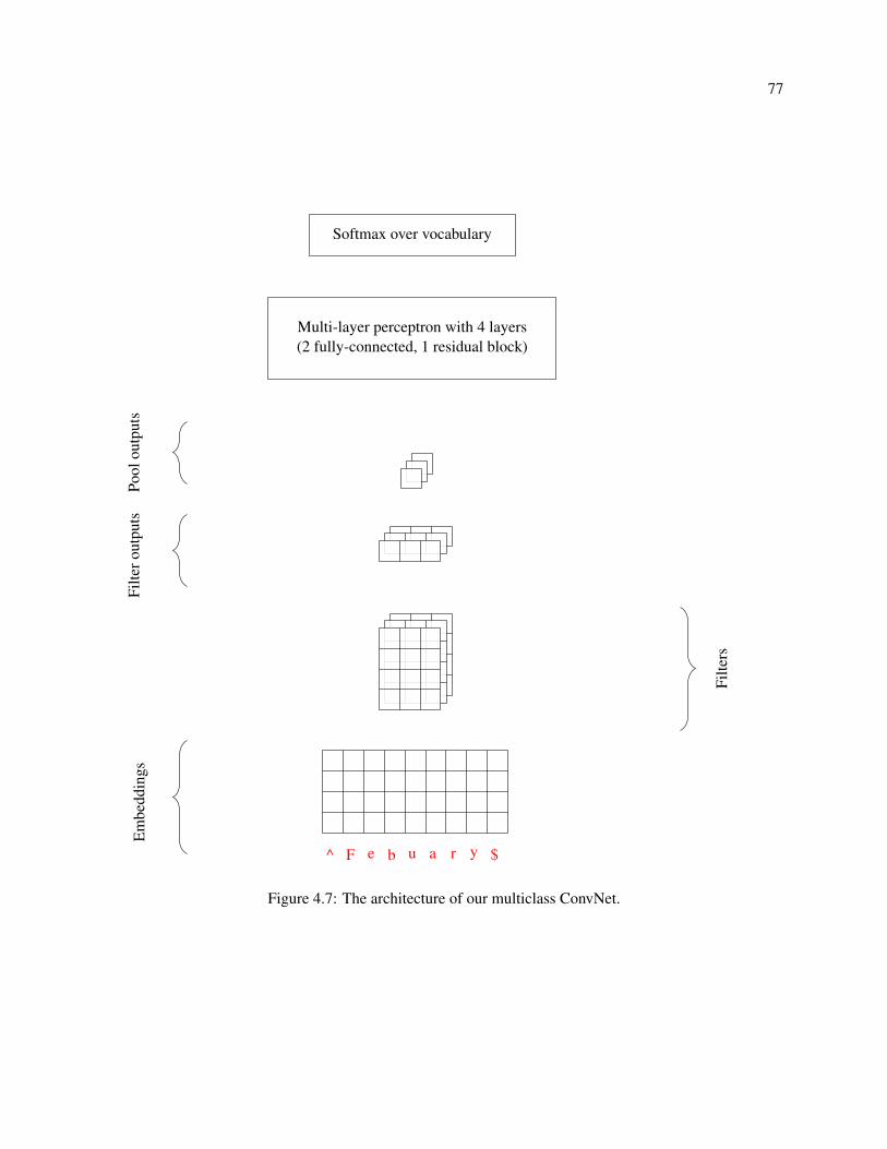
77

^ F e b u a r y $

Multi-layer perceptron with 4 layers(2 fully-connected, 1 residual block)

Softmax over vocabulary

Em

bedd

ings

Filte

rout

puts

Pool

outp

uts

Filte

rs

Figure 4.7: The architecture of our multiclass ConvNet.

78

of the units in order for the layers of the network to begin to collaborate.

Once we set the batch size to 1024, the network began to learn. We trained the ConvNet for 1217

epochs with early stopping with a patience of 100 epochs. When it terminated, it had achieved an F1 on the

validation set of 0.94 compared to Jaro-Winkler’s 0.87.

For brevity, we present only the results on the Mitton corpora, which can be seen in Table 4.8. At rank

K = 1, the ConvNet outperforms Jaro-Winkler for all corpora but the challenging Holbrook corpus. For

rank K > 1, the Jaro-Winkler is the better approach. This aspect of the model’s performance is somewhat

surprising; we had assumed that a good ranking would spontaneously emerge from the simultaneous training

of the units in the output layer. We speculate that the failure of this model to perform well at K > 1 is a

consequence of the model being trained with categorical cross-entropy loss instead of a ranking loss. One

way this may be remedied is by augmenting the network with a multiclass linear output layer with a loss that

is the mean-squared error of the Damerau-Levenshtein distance between the non-word input and the output

of the layer. The question is beyond the scope of this investigation. In the rest of this dissertation we focus

only on ConvNets that implement the RANK interface.

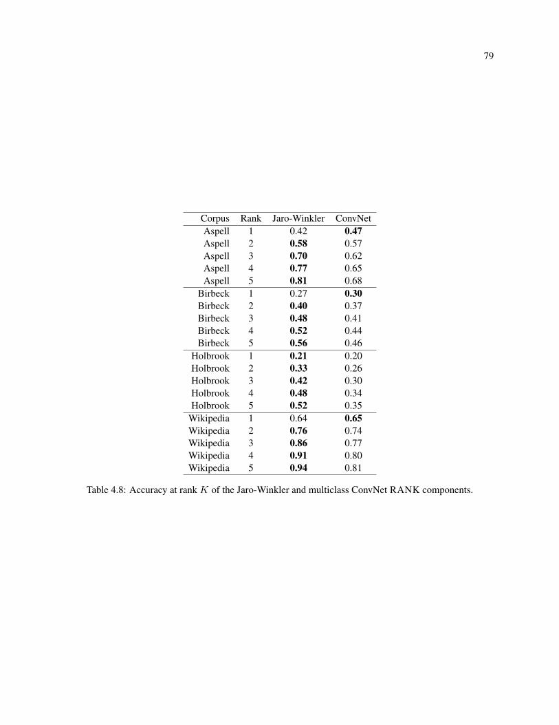
79

Corpus Rank Jaro-Winkler ConvNetAspell 1 0.42 0.47Aspell 2 0.58 0.57Aspell 3 0.70 0.62Aspell 4 0.77 0.65Aspell 5 0.81 0.68

Birbeck 1 0.27 0.30Birbeck 2 0.40 0.37Birbeck 3 0.48 0.41Birbeck 4 0.52 0.44Birbeck 5 0.56 0.46

Holbrook 1 0.21 0.20Holbrook 2 0.33 0.26Holbrook 3 0.42 0.30Holbrook 4 0.48 0.34Holbrook 5 0.52 0.35

Wikipedia 1 0.64 0.65Wikipedia 2 0.76 0.74Wikipedia 3 0.86 0.77Wikipedia 4 0.91 0.80Wikipedia 5 0.94 0.81

Table 4.8: Accuracy at rank K of the Jaro-Winkler and multiclass ConvNet RANK components.

80

4.5 Conclusion

In this chapter we evaluated the performance of ConvNets on isolated non-word error correction. The

results indicate that ConvNets are able to learn to rank candidate lists somewhat better than a standard string

metric-based approach. A natural interpretation of these results is that the ConvNet itself learns a string

metric. We believe that the key difference between Jaro-Winkler distance and the ConvNet is that the string

metric learned by the ConvNet is conditioned by data. This conditioning, we conjecture, allows the model

to rank candidate lists differently depending on the inputs.

We also compared ConvNets to a Random Forest RANK model and found the latter to significantly

outperform the former. The feature set with which the Random Forest model is trained includes the unigram

probability of a candidate. The unigrams are taken from a corpus of 1-5 grams extracted from a corpus of

~1 trillion words. This gives the Random Forest model a distinct advantage of being able to assign lower

rank to candidate words that are rarely used. This comparison differs from those reported in Chapters 3

and 5 in that in the other chapters the features used to train the ConvNet and probabilistic language models

are the same, whereas in this chapter the Random Forest RANK model has an additional language model

feature. The result indicates that significant performance gains can be obtained by using contextual features

and motivates our use of contextual features in the next chapter.

None of the approaches evaluated in this chapter meet the interactive and automatic correction per-

formance requirements of 95% top-5 accuracy and 99% top-1 accuracy that we laid out in Chapter 1. This

comes with a qualification. When test examples are separated by the length of the non-word and accuracies

are computed over non-words of a given length, as in Figure 4.4, we see that the model performs nearly

adequately on non-words of length 10 or greater. We will focus in the next chapter on words of length 3-4

characters, on the grounds that if we can achieve satisfactory performance with them, we will be able to do

the same with all longer words.

Chapter 5

Study 3: Contexual Non-word Error Correction

In the previous chapter we explored the limits of isolated non-word error correction and found that a

strong supervised baseline – the Random Forest mode – that makes use of unigram language model prob-

abilities tends to be a better RANK component than either Jaro-Winkler distance or a binary ConvNet.

Informed by these results, we now turn our attention to ConvNets that make use of the context non-word

errors. We also previously found that while a multiclass ConvNet has slightly better accuracy at K = 1 than

Jaro-Winkler distance, it’s performance at K > 1 is consistently much worse; consequently, in this chapter

we will focus only on a binary classification ConvNet that implements the RANK interface.

As we also saw in the previous chapter, correction difficulty is inversely proportional to non-word

length. Shorter words are more difficult to correct for several reasons.

(1) Since they are made of fewer characters, there is simply less information in the error.

(2) All else being equal, the fraction of information that is lost when a word is misspelled is greater for

shorter words.

(3) The number of words that can be reached by a single edit operation is greater [Pet80].

In this chapter, then, we will focus on shorter words of 3-4 characters. Since spelling correction

systems tend to perform least well on them, they are in greatest need of improvement.

Shorter words lend themselves less well to the generative approach used to create the training data

for the models described in the previous Chapter. Shorter words have fewer characters, which implies fewer

opportunities to apply edits in a generative fashion.

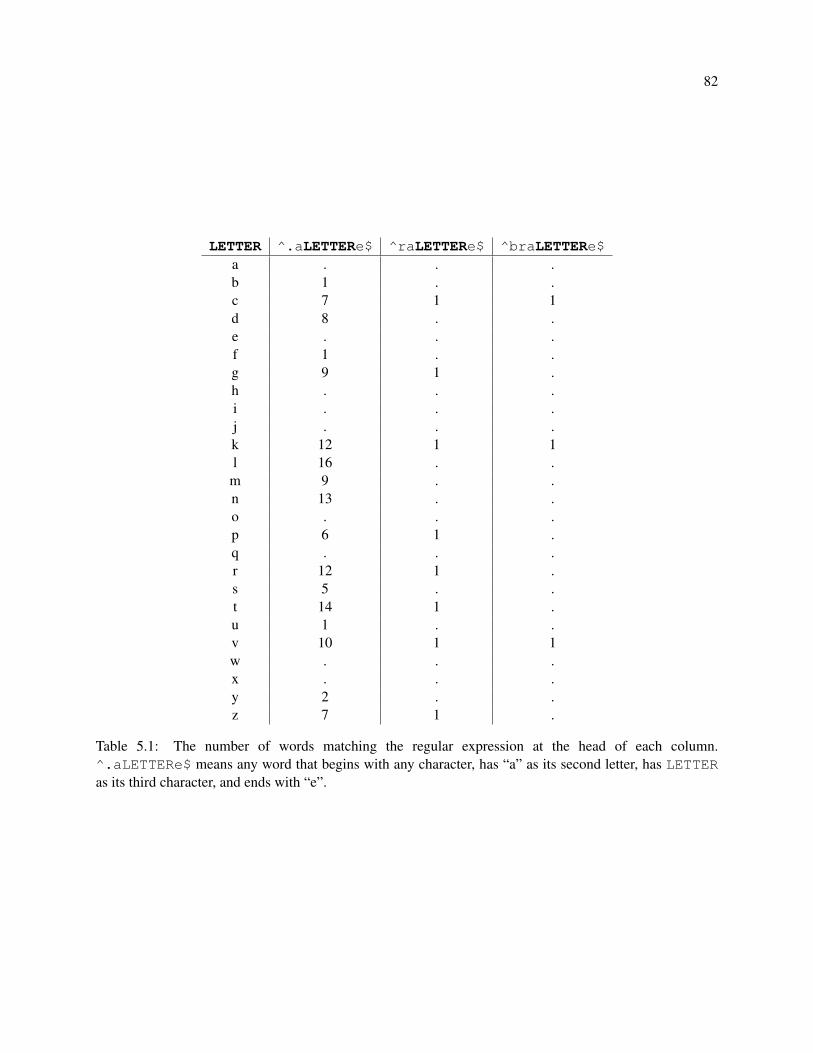
82

LETTER ^.aLETTERe$ ^raLETTERe$ ^braLETTERe$a . . .b 1 . .c 7 1 1d 8 . .e . . .f 1 . .g 9 1 .h . . .i . . .j . . .k 12 1 1l 16 . .

m 9 . .n 13 . .o . . .p 6 1 .q . . .r 12 1 .s 5 . .t 14 1 .u 1 . .v 10 1 1w . . .x . . .y 2 . .z 7 1 .

Table 5.1: The number of words matching the regular expression at the head of each column.^.aLETTERe$ means any word that begins with any character, has “a” as its second letter, has LETTERas its third character, and ends with “e”.

83

5.1 Corpus

Training and evaluating a model for contextual non-word error correction requires a corpus both of

non-words and contexts. For contexts, we extracted a corpus of ~44m sentences from English Wikipedia.

For non-words, we used the generative process described in Section 4.1.0.2. The generative model was

trained using the Aspell, Birbeck, Holbrook, and Wikipedia corpora (see Section 4.1.0.1 for details). We

chose a set of 1,686 3-4 character words from the Aspell English dictionary for which we were able to find

at least 100 occurrences in the corpus of sentences.

For each word, we sampled 100 or more sentences containing the word; if there were more than

1000 sentences, we randomly sampled 1000, so every word had between 100-1000 sentences containing an

example of its use. Then for each (word, sentence) tuple, we then extracted the window of 5 words centered

on the word. The result was a set of 1,490,280 (word, context) tuples.

We took additional steps that prevented leakage of training data into the test set to ensure parity of

vocabulary among the vocabulary of our models and our language model baseline. To prevent leakage, we

eliminated duplicate contexts. This reduced the number of tuples to 1,384,477.

We then eliminated contexts with words outside the the Aspell English dictionary; 954,246 contexts

remained.

5.2 Models

In this section we describe the models we used in our experiments. All of the models implement

the RANK interface, meaning they take a non-word and a candidate list and rank the list according to an

explicit or implicit scoring function. The RETRIEVE component used to provide the candidate lists is the

combined Aspell and near-miss RETRIEVE component described in Section 4.2.

5.2.1 Google Web 1T 5-gram Language Model RANK

A common implementation of a RANK component for context-dependent error correction ranks a

candidates according to the probability of the context of the non-word when the non-word has been replaced

84

by the candidate. Obtaining the probability of the context requires a language model. The language model

we use for this model is trained using n-grams for 1 ≤ n ≤ 4 from Version 1 of the Google Web 1T 5-gram

corpus 1 , good-Turing discounting, and Katz backoff.

5.2.2 Context-Dependent ConvNets RANK

The networks described in this section are ConvNets that make use of either the lexical context of a

non-word (Word ConvNet) or both the lexical context and the non-word itself (Word and Character Con-

vNet). Lexical context is processed by a lexical convolutional block, which consists of a word embedding

matrix, a set of convolutional filters, and a max pooling layer. The non-word context is processed by a char-

acter convolutional block that has the same basic components as the lexical block, except the embeddings

are characters.

A lexical block in a network was set up to take inputs of exactly 5 words. Given an example (word,

context) tuple, a non-word was created using the generative model and a candidate list was obtained from the

RETRIEVE component. Then each candidate was substituted for the non-word in the middle of the context;

the target variable was set to 1 if the candidate was the true correction and 0 otherwise. The filters of this

block were of width 5. The max pooling layer of this block was therefore effectively an identity function;

the model could have been trained without it. This block had 1000 convolutional filters and 50-dimensional

word embeddings.

A character block took inputs of 6 characters, had filters of width 4, and 25-dimensional character

embeddings. There were 100 character filters.

Finally, the networks had a stack of four fully-connected residual blocks with 100 units each [He+15],

followed by a softmax layer. The input to the first layer of the Word ConvNet’s residual stack was 1000

dimensions, equal to the number of filters in the lexical block. In the Word and Character ConvNet, the input

to the residual stack was 1200 dimensions, with the additional 200 dimensions coming from the character

convolutional block’s output for both the non-word and the candidate word.1 https://catalog.ldc.upenn.edu/LDC2006T13

85

5.2.3 Feed-Forward Embedding Network RANK

Since the width lexical contexts used to train the ConvNets described in the previous section were

fixed, it is possible to compare them to an ordinary feed-forward neural network with a word embedding

layer in which the word embeddings are simply concatenated and passed to a fully-connected layer as a

feature vector. This comparison gives a sense of the trade-off between performance and the number of

parameters.

The feed-forward network we used took windows of width 5 as input and had 200-dimensional word

embeddings. For a single context, the concatenation of the word embeddings resulted in a 1000-dimensional

feature vector, the same size as the output of the lexical convolutional block. As with the ConvNets, this

network had four fully-connected residual blocks with 100 units each, then a softmax layer.

5.3 Experiments

For all models the non-linearities were rectified linear units. Models were trained with early stopping

using a patience of 50 epochs. Loss was computed using categorical cross entropy and scaled using Equation

3 with λ = 1. The Adam optimizer was used for computing updates to model parameters [KA15]. Of the

954,246 (word, context) tuples in our data set, we allocated 90% for training, 4,500 for validation, and the

remaining 80,386 for test. A given context could only appear in one of these data sets, so data leakage

of context did not occur. Since, however, non-words were generated by the same process for all data sets,

a non-word could appear in the training and test sets. During training and evaluation, the candidate lists

retrieved for all models and the Google Web 1T 5-gram corpus baseline were restricted to our vocabulary of

1,686 words.

We expected that the extra information provided by character-level inputs would give a Word and

Character ConvNet a slight advantage over the other models. However, since a given word and non-word

could appear in the training and test sets, it was possible for that model’s performance on test set examples

to be tainted by prior exposure of the character-level portion of the examples during training. To prevent

this model from memorizing (word, non-word) pairs and ignoring the context inputs, we added noise to

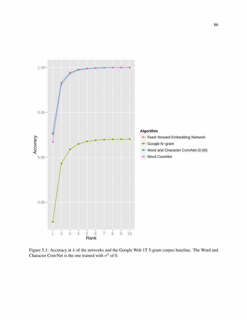
86

●

●

●

●● ● ● ● ● ●

●

●

●

●● ● ● ● ● ●

●

●

●

●● ● ● ● ● ●

●

●

●

●●

● ● ● ● ●

0.85

0.90

0.95

1.00

1 2 3 4 5 6 7 8 9 10Rank

Acc

urac

y

Algorithm

●

●

●

●

Feed−forward Embedding Network

Google N−gram

Word and Character ConvNet (0.00)

Word ConvNet

Figure 5.1: Accuracy at k of the networks and the Google Web 1T 5-gram corpus baseline. The Word andCharacter ConvNet is the one trained with σ2 of 0.

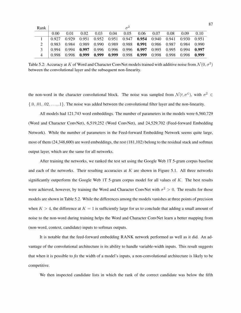
87Rank σ2

0.00 0.01 0.02 0.03 0.04 0.05 0.06 0.07 0.08 0.09 0.101 0.927 0.929 0.951 0.952 0.951 0.947 0.954 0.940 0.941 0.930 0.9512 0.983 0.984 0.989 0.990 0.989 0.988 0.991 0.986 0.987 0.984 0.9903 0.994 0.994 0.997 0.996 0.996 0.996 0.997 0.995 0.995 0.994 0.9974 0.998 0.998 0.999 0.999 0.999 0.998 0.999 0.998 0.998 0.998 0.999

Table 5.2: Accuracy at K of Word and Character ConvNet models trained with additive noise from N (0, σ2)between the convolutional layer and the subsequent non-linearity.

the non-word in the character convolutional block. The noise was sampled from N (′, σ∈), with σ2 ∈

{.0, .01, .02, . . . , .1}. The noise was added between the convolutional filter layer and the non-linearity.

All models had 121,743 word embeddings. The number of parameters in the models were 6,560,729

(Word and Character ConvNet), 6,519,252 (Word ConvNet), and 24,529,702 (Feed-forward Embedding

Network). While the number of parameters in the Feed-forward Embedding Network seems quite large,

most of them (24,348,600) are word embeddings, the rest (181,102) belong to the residual stack and softmax

output layer, which are the same for all networks.

After training the networks, we ranked the test set using the Google Web 1T 5-gram corpus baseline

and each of the networks. Their resulting accuracies at K are shown in Figure 5.1. All three networks

significantly outperform the Google Web 1T 5-gram corpus model for all values of K. The best results

were achieved, however, by training the Word and Character ConvNet with σ2 > 0. The results for those

models are shown in Table 5.2. While the differences among the models vanishes at three points of precision

when K > 4, the difference at K = 1 is sufficiently large for us to conclude that adding a small amount of

noise to the non-word during training helps the Word and Character ConvNet learn a better mapping from

(non-word, context, candidate) inputs to softmax outputs.

It is notable that the feed-forward embedding RANK network performed as well as it did. An ad-

vantage of the convolutional architecture is its ability to handle variable-width inputs. This result suggests

that when it is possible to fix the width of a model’s inputs, a non-convolutional architecture is likely to be

competitive.

We then inspected candidate lists in which the rank of the correct candidate was below the fifth

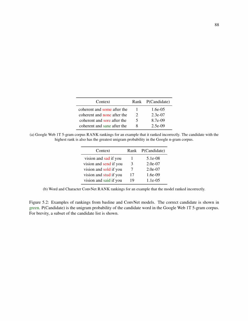
88

Context Rank P(Candidate)

coherent and some after the 1 1.6e-05coherent and none after the 2 2.3e-07coherent and sore after the 5 8.7e-09coherent and sane after the 8 2.5e-09

(a) Google Web 1T 5-gram corpus RANK rankings for an example that it ranked incorrectly. The candidate with thehighest rank is also has the greatest unigram probability in the Google n-gram corpus.

Context Rank P(Candidate)

vision and sad if you 1 5.1e-08vision and send if you 3 2.0e-07vision and sold if you 7 2.0e-07vision and stud if you 17 1.6e-09vision and said if you 19 1.1e-05

(b) Word and Character ConvNet RANK rankings for an example that the model ranked incorrectly.

Figure 5.2: Examples of rankings from basline and ConvNet models. The correct candidate is shown ingreen. P(Candidate) is the unigram probability of the candidate word in the Google Web 1T 5-gram corpus.For brevity, a subset of the candidate list is shown.

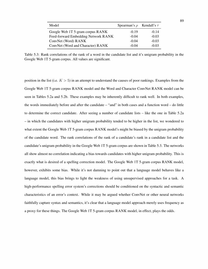
89Model Spearman’s ρ Kendall’s τ

Google Web 1T 5-gram corpus RANK -0.19 -0.14Feed-forward Embedding Network RANK -0.04 -0.03ConvNet (Word) RANK -0.04 -0.03ConvNet (Word and Character) RANK -0.04 -0.03

Table 5.3: Rank correlations of the rank of a word in the candidate list and it’s unigram probability in theGoogle Web 1T 5-gram corpus. All values are significant.

position in the list (i.e. K > 5) in an attempt to understand the causes of poor rankings. Examples from the

Google Web 1T 5-gram corpus RANK model and the Word and Character ConvNet RANK model can be

seen in Tables 5.2a and 5.2b. These examples may be inherently difficult to rank well. In both examples,

the words immediately before and after the candidate – “and” in both cases and a function word – do little

to determine the correct candidate. After seeing a number of candidate lists – like the one in Table 5.2a

– in which the candidates with higher unigram probability tended to be higher in the list, we wondered to

what extent the Google Web 1T 5-gram corpus RANK model’s might be biased by the unigram probability

of the candidate word. The rank correlations of the rank of a candidate’s rank in a candidate list and the

candidate’s unigram probability in the Google Web 1T 5-gram corpus are shown in Table 5.3. The networks

all show almost no correlation indicating a bias towards candidates with higher unigram probability. This is

exactly what is desired of a spelling correction model. The Google Web 1T 5-gram corpus RANK model,

however, exhibits some bias. While it’s not damning to point out that a language model behaves like a

language model, this bias brings to light the weakness of using unsupervised approaches for a task. A

high-performance spelling error system’s corrections should be conditioned on the syntactic and semantic

characteristics of an error’s context. While it may be argued whether ConvNet or other neural networks

faithfully capture syntax and semantics, it’s clear that a language model approach merely uses frequency as

a proxy for these things. The Google Web 1T 5-gram corpus RANK model, in effect, plays the odds.

90

5.4 Conclusion

The results of the experiments in this chapter show that ConvNets can outperform traditional language-

model approaches to context-dependent non-word error correction. That these performance gains were

achieved on words of 3-4 characters, which are notoriously difficult to correct, highlights the effectiveness

of this approach. The improvements of performance are particularly striking when one considers that the

number of 5-gram contexts used to train the networks is an order of magnitude smaller than the number of

5-grams in the Web 1T 5-gram corpus.

Chapter 6

Study 4: Correcting Preposition Errors with Convolutional Networks and Contrasting

Cases

Grammatical error detection and correction are key components of many educational applications.

Detecting errors is useful in writing evaluation systems, such as automated essay scoring, particularly when

the number and kind of grammatical errors contribute to the score. Automatically correcting errors increases

the utility of interactive applications. An interactive writing tutoring system, for example, may have an error

correction module that shows a learner how to improve their writing by suggesting how to correct errors it

has detected.

Detection and correction of grammatical errors that are a function of single word choice – such as

article selection, preposition selection, confusable words, and real-word spelling errors – can be performed

by an n-way classifier that predicts the correct word wpred ∈ C given some input word wactual ∈ C, where

C is a confusion set and n = |C|. Error detection is performed by reducing the n-way classifier to a binary

classifier; if wpred and wactual differ, the model is said to have detected an error. A writing tutoring system

– to continue with the previous application example – can highlight a detected error, thereby giving the

learner an opportunity to correct it. If the learner needs further assistance, the system can present wpred to

the learner as a proposed correction or provide additional directed training1 .1 In the remainder of this paper, we will use correction to refer to both detection and correction, except when required for clarity.

92

6.1 Feature Engineering Versus Learning

To date, the development of systems for correcting preposition errors has involved feature engineer-

ing, which is the process of designing and implementing modules that transform raw data into information-

rich values that can be input to a statistical model in order to perform some task. Such features are not

necessarily engineered from scratch; they may be the output of some other system, such as a part-of-speech

tagger or a parser. A preposition error correction model may, for instance, be trained with a feature set

that includes a window of tokens centered on a preposition, their corresponding part-of-speech tags, Word-

Net attributes, and other engineered features. The number of features in published descriptions of systems

ranges from about 25 [HCL04; CTH07; TC08a; TC08b; Han+10; TFC10] to more than 300 [DP07]. Pars-

ing (“deep”) and n-gram (“shallow”) approaches have been compared using an artificial corpus of errors

[WFG07]. To be clear, not all of the features used in these systems require feature engineering, properly

speaking. Indeed, the tokens in the window around the preposition can be considered raw data.

An alternative to feature engineering is feature learning. In this approach, raw data are input directly

to a statistical model. The model itself contains a set of parameters structured according to prior knowledge

about the domain. For a natural language processing task such as preposition correction, one set of parame-

ters may represent the words in the model’s vocabulary, and a higher-order set of parameters may represent

sequences of words. Implicit in this approach is the assumption that, for supervised learning tasks, there is

enough information in the raw inputs alone to learn a good mapping from the inputs to the target variable.

A notable difference between feature engineering and feature learning is the way raw inputs – se-

quences of tokens – are represented. Commonly, in a feature engineering setting, a single token is repre-

sented using an indicator or one-hot vector. A one-hot vector has one element for every word in the vocab-

ulary; the element corresponding to the token’s type is 1, and all other elements are 0. In a feature learning

setting, by contrast, a word is often represented as a real-valued vector – a distributed word representation

or embedding.

One-hot word representations have a significant deficiency: they preclude the distributional hypoth-

esis [Fir57], which states, in effect, that similar words will be found in similar contexts. With one-hot

93

representations, feature vectors are disjoint and permit no variance in similarity; the one-hot representations

for doctor and physician are just as similar as those of paintbrush and catapult. With distributed embed-

dings, however, doctor is geometrically near physician. Consequently, distributed word embeddings may

help supervised models generalize better because they allow the model to learn to detect approximate, fuzzy

patterns. Using word embeddings, a model trained with a data set that contains several occurrences of a

phrase – for instance, “Frog ate lunch” – may also be able to detect similar but previously unseen phrases,

such as “Toad ate breakfast”, solely because of the Frog-Toad and lunch-breakfast similarities.

Recent results have demonstrated that neural networks equipped with feature learning layers can

achieve high accuracy on very complex tasks [KSH12; GMH13]. This paper presents results from studies

that bring neural networks to bear on the problem of grammatical error correction. Their purpose is to de-

termine whether a feature learning approach is sufficient to achieve performance comparable to previously-

reported results on native writing.

This investigation is limited to preposition selection errors resulting from the incorrect choice from

the confusion set C of nine common prepositions – namely, “at”, “by”, “for”, “from”, “in”, “of”, “on”, “to”,

and “with”. In the concluding section of this paper, we discuss extending the approach presented here so it

can be evaluated on corpora of learner errors, which in addition include extraneous and missing preposition

errors. This work nonetheless may generalize to other word selection tasks, such as correcting confusable

words and real-word spelling errors (e.g. except/accept, quiet/quite) [Kuk92b].

6.2 ConvNets with Contrasting Cases

In our experiments, we train convolutional neural networks (ConvNets) [Lec+98; CW08a] to correct

preposition errors using a corpus of contrasting cases, a concept from educational research. In the contrast-

ing cases literature, it is argued that comparison of examples “support[s] transfer by helping people abstract

the key features of the method so that it is not tied to overly narrow problem features” [RS11]. Contrasting

cases function in a similar manner for our models. In our approach, a contrasting case is a pair of examples.

One is a real sentence from some corpus; the other, a negative example, is the same sentence in which the

preposition in the position being considered has been replaced by a randomly-selected preposition from the

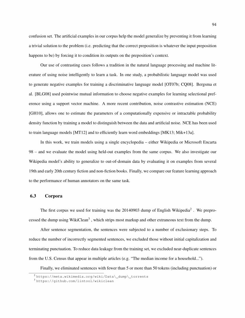
94

confusion set. The artificial examples in our corpus help the model generalize by preventing it from learning

a trivial solution to the problem (i.e. predicting that the correct preposition is whatever the input preposition

happens to be) by forcing it to condition its outputs on the preposition’s context.

Our use of contrasting cases follows a tradition in the natural language processing and machine lit-

erature of using noise intelligently to learn a task. In one study, a probabilistic language model was used

to generate negative examples for training a discriminative language model [OT07b; CQ08]. Bergsma et

al. [BLG08] used pointwise mutual information to choose negative examples for learning selectional pref-

erence using a support vector machine. A more recent contribution, noise contrastive estimation (NCE)

[GH10], allows one to estimate the parameters of a computationally expensive or intractable probability

density function by training a model to distinguish between the data and artificial noise. NCE has been used

to train language models [MT12] and to efficiently learn word embeddings [MK13; Mik+13a].

In this work, we train models using a single encyclopedia – either Wikipedia or Microsoft Encarta

98 – and we evaluate the model using held-out examples from the same corpus. We also investigate our

Wikipedia model’s ability to generalize to out-of-domain data by evaluating it on examples from several

19th and early 20th century fiction and non-fiction books. Finally, we compare our feature learning approach

to the performance of human annotators on the same task.

6.3 Corpora

The first corpus we used for training was the 20140903 dump of English Wikipedia2 . We prepro-

cessed the dump using WikiClean3 , which strips most markup and other extraneous text from the dump.

After sentence segmentation, the sentences were subjected to a number of exclusionary steps. To

reduce the number of incorrectly segmented sentences, we excluded those without initial capitalization and

terminating punctuation. To reduce data leakage from the training set, we excluded near-duplicate sentences

from the U.S. Census that appear in multiple articles (e.g. “The median income for a household...”).

Finally, we eliminated sentences with fewer than 5 or more than 50 tokens (including punctuation) or2 https://meta.wikimedia.org/wiki/Data\_dump\_torrents3 https://github.com/lintool/wikiclean

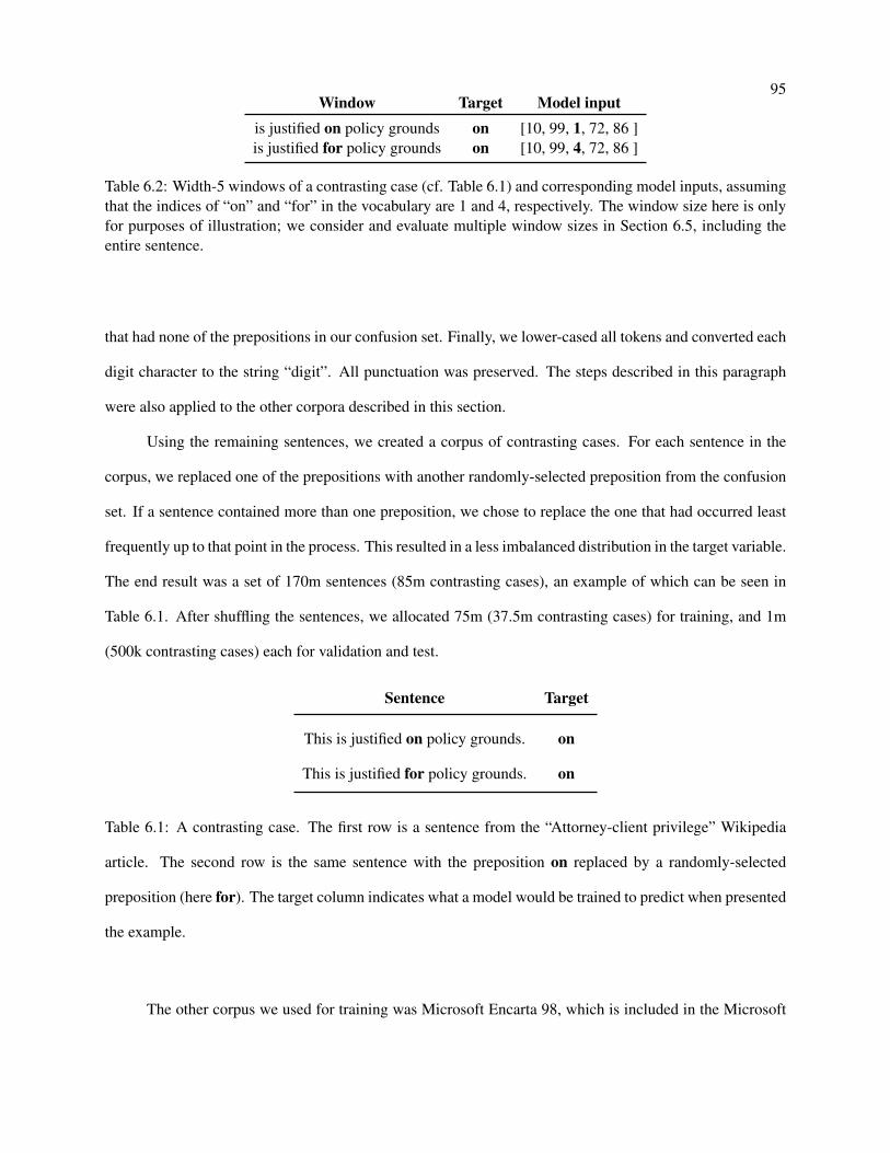
95Window Target Model input

is justified on policy grounds on [10, 99, 1, 72, 86 ]is justified for policy grounds on [10, 99, 4, 72, 86 ]

Table 6.2: Width-5 windows of a contrasting case (cf. Table 6.1) and corresponding model inputs, assumingthat the indices of “on” and “for” in the vocabulary are 1 and 4, respectively. The window size here is onlyfor purposes of illustration; we consider and evaluate multiple window sizes in Section 6.5, including theentire sentence.

that had none of the prepositions in our confusion set. Finally, we lower-cased all tokens and converted each

digit character to the string “digit”. All punctuation was preserved. The steps described in this paragraph

were also applied to the other corpora described in this section.

Using the remaining sentences, we created a corpus of contrasting cases. For each sentence in the

corpus, we replaced one of the prepositions with another randomly-selected preposition from the confusion

set. If a sentence contained more than one preposition, we chose to replace the one that had occurred least

frequently up to that point in the process. This resulted in a less imbalanced distribution in the target variable.

The end result was a set of 170m sentences (85m contrasting cases), an example of which can be seen in

Table 6.1. After shuffling the sentences, we allocated 75m (37.5m contrasting cases) for training, and 1m

(500k contrasting cases) each for validation and test.

Sentence Target

This is justified on policy grounds. on

This is justified for policy grounds. on

Table 6.1: A contrasting case. The first row is a sentence from the “Attorney-client privilege” Wikipedia

article. The second row is the same sentence with the preposition on replaced by a randomly-selected

preposition (here for). The target column indicates what a model would be trained to predict when presented

the example.

The other corpus we used for training was Microsoft Encarta 98, which is included in the Microsoft

96

Research Question-Answering Corpus 4 . The sentences in the corpus were already segmented. Unlike the

Wikipedia corpus, where we considered only one preposition per sentence, with Encarta we considered all

prepositions in our confusion set. Using a subset of ∼1250k preposition contexts, we allocated 300k for

train, 50k for validation, and the remaining ∼900k for test. From the 300k training contexts, we created

contrasting cases, yielding 600k examples. Since we wished to determine how well the model performs

with relatively few training examples, we opted only to use 300k examples (150k contrasting cases) out of

those 600k for training. For consistency with previous work [Gam+08; TC08a], we used only real examples

for validation and test.

For out-of-domain evaluation, we obtained eight books from Project Gutenberg 5 . Before sentence

segmentation, we removed the Project Gutenberg header and footer from each book.

The vocabularies for the models described in Section 6.5 were selected from the training sets. A

word in the vocabulary had to occur at least 5 times in the training set and the vocabulary was not allowed

to exceed 100k words. The Wikipedia-based model vocabulary came from the first 1m of the 75m examples

in the training set. The size of the Wikipedia and Encarta vocabularies were 83064 and 40659 words,

respectively. Out-of-vocabulary words were replaced with an “unknown word” token.

6.4 Modeling

We use a ConvNet architecture commonly applied to natural language processing tasks [CW08a;

Kim14a]. In this architecture, a ConvNet has (1) a word embedding layer, (2) a temporal convolutional layer

containing a set of filters, (3) a max pooling layer for reducing the variable-width convolutional output to a

fixed width, and (4) a sequence of one or more fully-connected layers. Specifics about the hyperparameters

of our models, which employ this general architecture, are provided in Section 6.5. The computational

mechanics of ConvNets are covered well in the original ConvNet paper [Lec+98].

An advantage of ConvNets is that they can be trained to model precise sequential patterns. Consider

a ConvNet trained using examples that are fixed-width windows centered on any of the prepositions in our4 http://research.microsoft.com/en-us/downloads/88c0021c-328a-4148-a158-a42d7331c6cf/5 https://www.gutenberg.org/

97

confusion set. Assume for simplicity that the filters are the same width as the model’s input. During training,

the word embedding layer and the filters in the convolutional layer collude to find a good configuration. In

the embedding layer, prepositions are pulled apart or pushed together depending on where the convolutional

layer needs them to be in order to reduce the model’s cost. In the convolutional layer, certain filters are

guided to specialize in certain prepositions and their contexts; the middle component of each filter will be

led to activate more highly on certain prepositions and the other components will learn to detect patterns

that occur in the fixed-width window around the prepositions. Thus, from a feature learning perspective,

ConvNets are appropriate for preposition error correction.

We train our models with many more parameters than examples; this increases the risk of overfitting.

Indeed, in this regime a model can learn the trivial solution, which is to ignore a preposition’s context and

predict whatever preposition happens to be present. To solve this problem, some regularization is necessary.

Instead of regularizing the model’s parameters using a technique such as weight decay or dropout [Hin+12],

we regularize the training examples. Our use of contrasting cases prevents the model from learning a trivial

solution by forcing it to pay attention to the context. Since a contrasting case has one artificial example

for every real example, the model can easily attain an accuracy of .5 by learning the trivial solution. Both

examples in a contrasting case have the same target variable, and their inputs differ only by one preposition,

so further gains in accuracy can only be achieved by paying attention to the context.

Concretely, consider the fixed-width windows of the constrasting case in Table 6.2. If a model is

trained with only real examples, the convolutional filters can learn to detect the “on” at the center of the

window and to pass that information on to the higher layers of the network. This trivial solution fails for the

artificial example, because copying the center word is guaranteed to result in an incorrect prediction. The

artificial examples thus force the model to condition itself on the non-obvious parts of the inputs.

6.5 Experiments

The experiments described in this section are designed to determine (1) how well a feature learning

approach performs on examples of preposition use from Wikipedia and Encarta, and (2) how well a model

trained using Wikipedia transfers out-of-domain preposition use (specifically, from 19th and early 20th

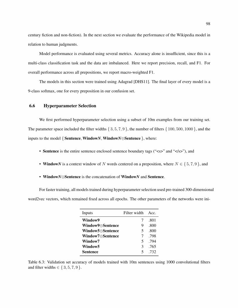
98

century fiction and non-fiction). In the next section we evaluate the performance of the Wikipedia model in

relation to human judgments.

Model performance is evaluated using several metrics. Accuracy alone is insufficient, since this is a

multi-class classification task and the data are imbalanced. Here we report precision, recall, and F1. For

overall performance across all prepositions, we report macro-weighted F1.

The models in this section were trained using Adagrad [DHS11]. The final layer of every model is a

9-class softmax, one for every preposition in our confusion set.

6.6 Hyperparameter Selection

We first performed hyperparameter selection using a subset of 10m examples from our training set.

The parameter space included the filter widths { 3, 5, 7, 9 }, the number of filters { 100, 500, 1000 }, and the

inputs to the model { Sentence, WindowN, WindowN⊕Sentence }, where:

• Sentence is the entire sentence enclosed sentence boundary tags (“<s>” and “</s>”), and

• WindowN is a context window of N words centered on a preposition, where N ∈ { 5, 7, 9 }, and

• WindowN⊕Sentence is the concatenation of WindowN and Sentence.

For faster training, all models trained during hyperparameter selection used pre-trained 300-dimensional

word2vec vectors, which remained fixed across all epochs. The other parameters of the networks were ini-

Inputs Filter width Acc.

Window9 7 .801Window9⊕Sentence 9 .800Window5⊕Sentence 5 .800Window7⊕Sentence 7 .798Window7 5 .794Window5 3 .765Sentence 5 .732

Table 6.3: Validation set accuracy of models trained with 10m sentences using 1000 convolutional filtersand filter widths ∈ { 3, 5, 7, 9 }.

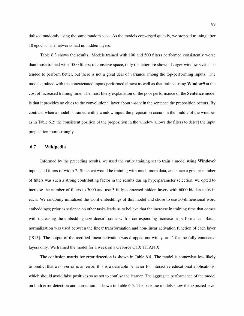
99

tialized randomly using the same random seed. As the models converged quickly, we stopped training after

10 epochs. The networks had no hidden layers.

Table 6.3 shows the results. Models trained with 100 and 500 filters performed consistently worse

than those trained with 1000 filters; to conserve space, only the latter are shown. Larger window sizes also

tended to perform better, but there is not a great deal of variance among the top-performing inputs. The

models trained with the concatenated inputs performed almost as well as that trained using Window9 at the

cost of increased training time. The most likely explanation of the poor performance of the Sentence model

is that it provides no clues to the convolutional layer about where in the sentence the preposition occurs. By

contrast, when a model is trained with a window input, the preposition occurs in the middle of the window,

as in Table 6.2; the consistent position of the preposition in the window allows the filters to detect the input

preposition more strongly.

6.7 Wikipedia

Informed by the preceding results, we used the entire training set to train a model using Window9

inputs and filters of width 7. Since we would be training with much more data, and since a greater number

of filters was such a strong contributing factor in the results during hyperparameter selection, we opted to

increase the number of filters to 3000 and use 3 fully-connected hidden layers with 6000 hidden units in

each. We randomly initialized the word embeddings of this model and chose to use 50-dimensional word

embeddings; prior experience on other tasks leads us to believe that the increase in training time that comes

with increasing the embedding size doesn’t come with a corresponding increase in performance. Batch

normalization was used between the linear transformation and non-linear activation function of each layer

[IS15]. The output of the rectified linear activation was dropped out with p = .5 for the fully-connected

layers only. We trained the model for a week on a GeForce GTX TITAN X.

The confusion matrix for error detection is shown in Table 6.4. The model is somewhat less likely

to predict that a non-error is an error; this is a desirable behavior for interactive educational applications,

which should avoid false positives so as not to confuse the learner. The aggregate performance of the model

on both error detection and correction is shown in Table 6.5. The baseline models show the expected level

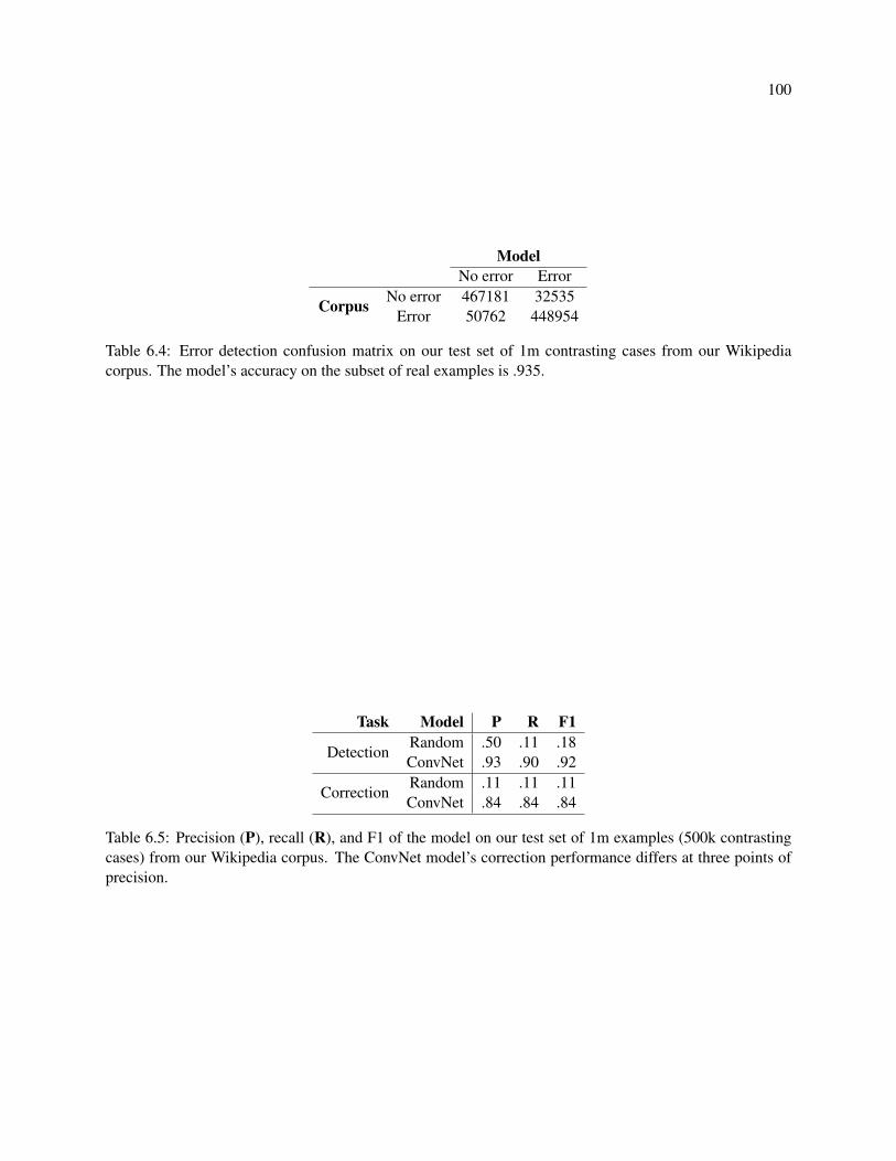
100

ModelNo error Error

Corpus No error 467181 32535Error 50762 448954

Table 6.4: Error detection confusion matrix on our test set of 1m contrasting cases from our Wikipediacorpus. The model’s accuracy on the subset of real examples is .935.

Task Model P R F1

DetectionRandom .50 .11 .18ConvNet .93 .90 .92

CorrectionRandom .11 .11 .11ConvNet .84 .84 .84

Table 6.5: Precision (P), recall (R), and F1 of the model on our test set of 1m examples (500k contrastingcases) from our Wikipedia corpus. The ConvNet model’s correction performance differs at three points ofprecision.

101

of peformance when the predicted preposition wpred is selected by choosing randomly from C.

Learner writing often contains spelling errors and neologisms. The vocabulary of a mdoel is typically

fixed once it is deployed. Unknown words – erroneous or not – become unknown words to a model. To

understand the effect of unknown words, we performed a sensitivity analysis using a sample of 50,000 test

set sentences that contain no unknown words. We were particularly interested in the joint effect of the

number of unknown words and their proximity to the preposition that the model is asked to evaluate. Let

S = { −2, −1, 1, 2 } be the set of positions of words in proximity to some preposition wactual. P(S) is the

power set of S. For the sensitivity analysis, we chose p ∈ P(S), set the words in the positions p for each of

the 50,000 sentences to be the unknown word, and evaluated the model’s performance using the perturbed

sentences.

Table 6.6 shows the results grouped row-wise by the number of unknown words. Performance de-

grades severely when words in the window are unknown. The degradation is proportional to proximity to the

preposition. A clear lesson from this is that a production error correction system should not be allowed to

suggest a correction if the window contains an unknown word. The degradation is asymmetrical in places.

When only one word in the window is unknown, the degradation is greater at position 2 than position -

2. Similarly, when two words are unknown, the degradation is greater for the position set { −1, 2 } than

{ −2, 1 }. This may indicate that making the trailing context longer than the leading context may help on

the preposition correction task.

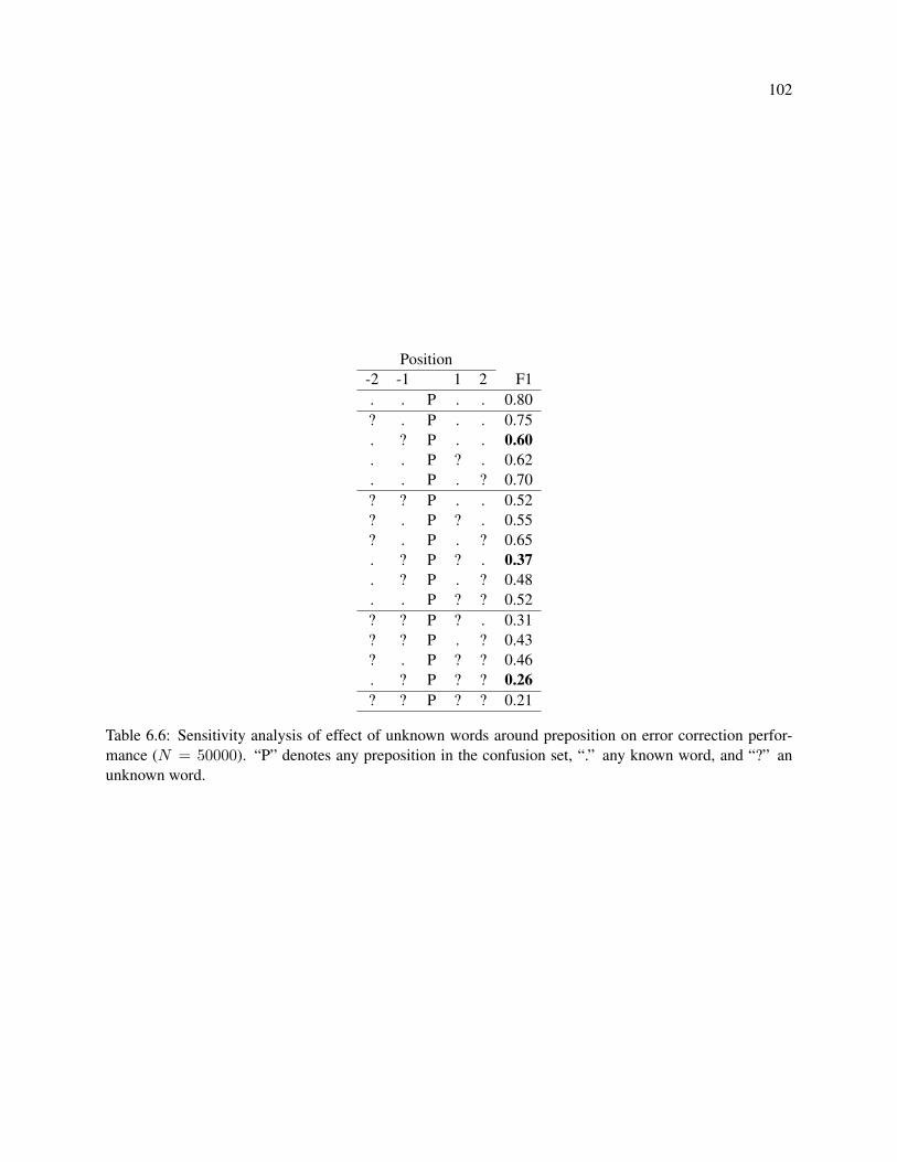
102

Position-2 -1 1 2 F1. . P . . 0.80? . P . . 0.75. ? P . . 0.60. . P ? . 0.62. . P . ? 0.70? ? P . . 0.52? . P ? . 0.55? . P . ? 0.65. ? P ? . 0.37. ? P . ? 0.48. . P ? ? 0.52? ? P ? . 0.31? ? P . ? 0.43? . P ? ? 0.46. ? P ? ? 0.26? ? P ? ? 0.21

Table 6.6: Sensitivity analysis of effect of unknown words around preposition on error correction perfor-mance (N = 50000). “P” denotes any preposition in the confusion set, “.” any known word, and “?” anunknown word.

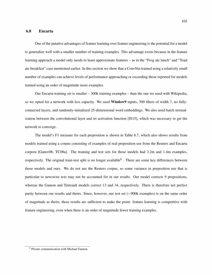
103

6.8 Encarta

One of the putative advantages of feature learning over feature engineering is the potential for a model

to generalize well with a smaller number of training examples. This advantage exists because in the feature

learning approach a model only needs to learn approximate features – as in the “Frog ate lunch” and “Toad

ate breakfast” case mentioned earlier. In this section we show that a ConvNet trained using a relatively small

number of examples can achieve levels of performance approaching or exceeding those reported for models

trained using an order of magnitude more examples.

Our Encarta training set is smaller – 300k training examples – than the one we used with Wikipedia,

so we opted for a network with less capacity. We used Window9 inputs, 300 filters of width 7, no fully-

connected layers, and randomly-initialized 25-dimensional word embeddings. We also used batch normal-

ization between the convolutional layer and its activation function [IS15], which was necessary to get the

network to converge.

The model’s F1 measure for each preposition is shown in Table 6.7, which also shows results from

models trained using a corpus consisting of examples of real preposition use from the Reuters and Encarta

corpora [Gam+08; TC08a]. The training and test sets for those models had 3.2m and 1.4m examples,

respectively. The original train-test split is no longer available6 . There are some key differences between

those models and ours. We do not use the Reuters corpus, so some variance in preposition use that is

particular to newswire text may not be accounted for in our results. Our model corrects 9 prepositions,

whereas the Gamon and Tetreault models correct 13 and 34, respectively. There is therefore not perfect

parity between our results and theirs. Since, however, our test set (∼900k examples) is on the same order

of magnitude as theirs, these results are sufficient to make the point: feature learning is competitive with

feature engineering, even when there is an order of magnitude fewer training examples.

6 Private communication with Michael Gamon.

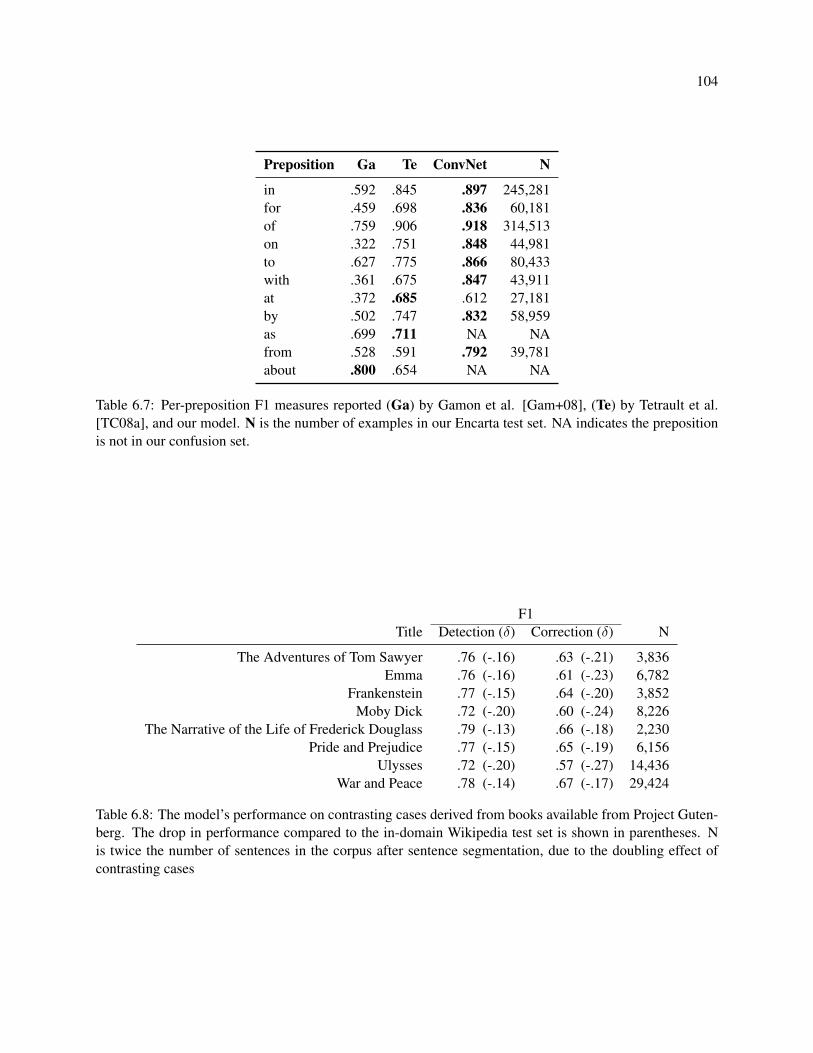
104

Preposition Ga Te ConvNet N

in .592 .845 .897 245,281for .459 .698 .836 60,181of .759 .906 .918 314,513on .322 .751 .848 44,981to .627 .775 .866 80,433with .361 .675 .847 43,911at .372 .685 .612 27,181by .502 .747 .832 58,959as .699 .711 NA NAfrom .528 .591 .792 39,781about .800 .654 NA NA

Table 6.7: Per-preposition F1 measures reported (Ga) by Gamon et al. [Gam+08], (Te) by Tetrault et al.[TC08a], and our model. N is the number of examples in our Encarta test set. NA indicates the prepositionis not in our confusion set.

F1Title Detection (δ) Correction (δ) N

The Adventures of Tom Sawyer .76 (-.16) .63 (-.21) 3,836Emma .76 (-.16) .61 (-.23) 6,782

Frankenstein .77 (-.15) .64 (-.20) 3,852Moby Dick .72 (-.20) .60 (-.24) 8,226

The Narrative of the Life of Frederick Douglass .79 (-.13) .66 (-.18) 2,230Pride and Prejudice .77 (-.15) .65 (-.19) 6,156

Ulysses .72 (-.20) .57 (-.27) 14,436War and Peace .78 (-.14) .67 (-.17) 29,424

Table 6.8: The model’s performance on contrasting cases derived from books available from Project Guten-berg. The drop in performance compared to the in-domain Wikipedia test set is shown in parentheses. Nis twice the number of sentences in the corpus after sentence segmentation, due to the doubling effect ofcontrasting cases

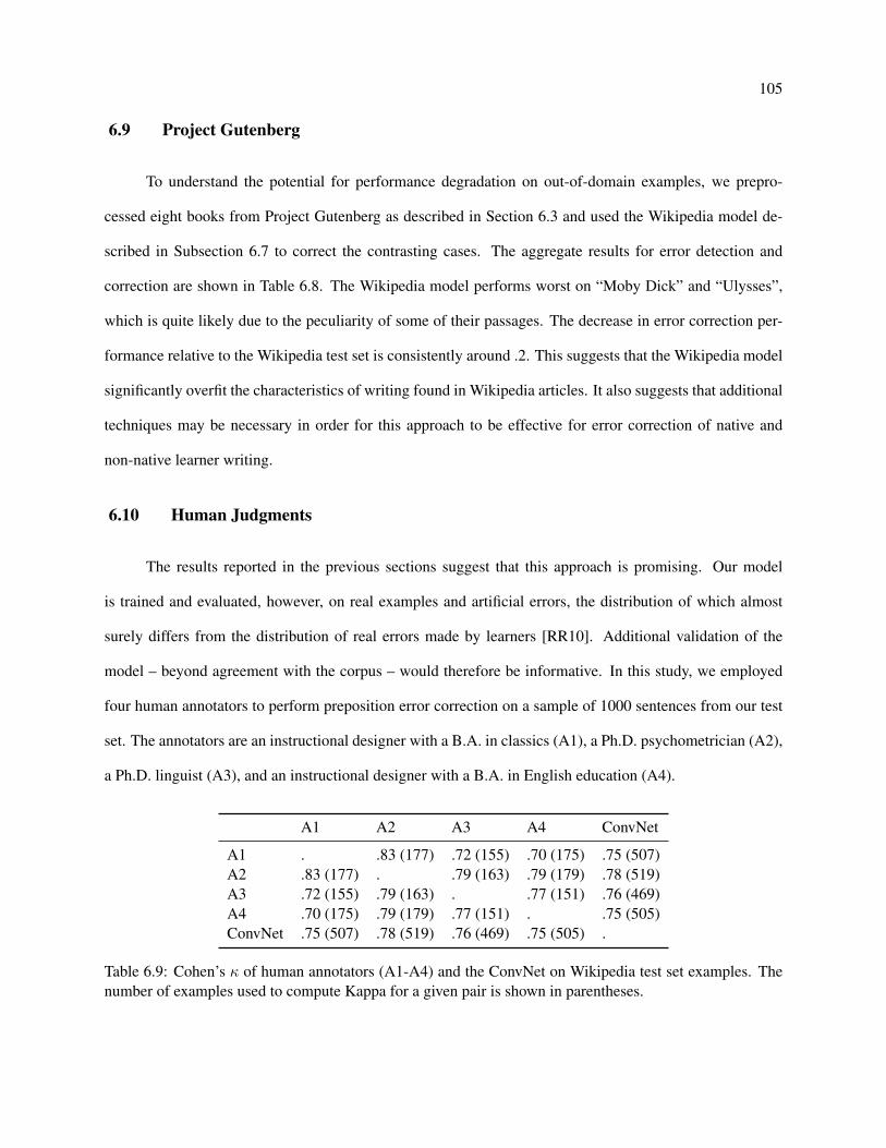
105

6.9 Project Gutenberg

To understand the potential for performance degradation on out-of-domain examples, we prepro-

cessed eight books from Project Gutenberg as described in Section 6.3 and used the Wikipedia model de-

scribed in Subsection 6.7 to correct the contrasting cases. The aggregate results for error detection and

correction are shown in Table 6.8. The Wikipedia model performs worst on “Moby Dick” and “Ulysses”,

which is quite likely due to the peculiarity of some of their passages. The decrease in error correction per-

formance relative to the Wikipedia test set is consistently around .2. This suggests that the Wikipedia model

significantly overfit the characteristics of writing found in Wikipedia articles. It also suggests that additional

techniques may be necessary in order for this approach to be effective for error correction of native and

non-native learner writing.

6.10 Human Judgments

The results reported in the previous sections suggest that this approach is promising. Our model

is trained and evaluated, however, on real examples and artificial errors, the distribution of which almost

surely differs from the distribution of real errors made by learners [RR10]. Additional validation of the

model – beyond agreement with the corpus – would therefore be informative. In this study, we employed

four human annotators to perform preposition error correction on a sample of 1000 sentences from our test

set. The annotators are an instructional designer with a B.A. in classics (A1), a Ph.D. psychometrician (A2),

a Ph.D. linguist (A3), and an instructional designer with a B.A. in English education (A4).

A1 A2 A3 A4 ConvNet

A1 . .83 (177) .72 (155) .70 (175) .75 (507)A2 .83 (177) . .79 (163) .79 (179) .78 (519)A3 .72 (155) .79 (163) . .77 (151) .76 (469)A4 .70 (175) .79 (179) .77 (151) . .75 (505)ConvNet .75 (507) .78 (519) .76 (469) .75 (505) .

Table 6.9: Cohen’s κ of human annotators (A1-A4) and the ConvNet on Wikipedia test set examples. Thenumber of examples used to compute Kappa for a given pair is shown in parentheses.

106

Each annotator was assigned approximately 500 sentences to correct. The sample given to an anno-

tator was constrained by two considerations. We wanted every sentence to receive two human judgments.

This ensured that we could compute inter-rater reliability using Cohen’s κ. We also wanted to be able to

compute κ using approximately the same number of sentences for each pair of annotators, so the distribution

of pairs of annotators across all sentences is approximately uniform.

Annotators were shown the entire sentence and the preposition to correct was rendered in bold font.

They were asked to select what they believed to be the correct preposition from a drop-down list. The results

are shown in Table 6.9. Overall, κ is quite high. The annotator-annotator κ values are less precise than the

annotator-model κ values, in that they are derived from a sample that is smaller by a factor of three. We note

that the range of agreement of the model with the annotators (.75-.78) is well within the range among all

pairings of annotators (.70-.83). There is also less variance in the annotator-model κ values. These results

indicate that the task can be performed reasonably well by humans and that the model performs on par with

humans.

6.11 Conclusion

Our results show that models trained by learning features are competitive with feature engineering

models. They also show that the models incur a noticeable degradation of performance on out-of-domain

examples. We introduced contrasting cases to address the problem of a ConvNet learning a trivial solution

when trained with real examples.

Since the distribution of errors in our corpus does not necessarily reflect the distribution of errors

made by learners [RR10], we evaluated our corpus against human judgments on a subset of the test set.

This analysis showed that there is little overall difference between the predictions of the models and the

judgments of annotators.

Many preposition error correction systems handle two kinds of errors that the exploratory system de-

scribed here does not – extraneous and missing prepositions. Our system currently only handles preposition

replacement errors. Replacement errors are more common than missing or extraneous word errors in one

corpus of errors [And07], so we believe our initial investigation is an important contribution to the field.

107

We nonetheless intend to enhance our system in the future to handle extraneous and missing prepositions.

We also intend to expand the kind of errors the system can correct and to evaluate it using recently-released

human-annotated error correction datasets [DK11; Ng+14a; Ng+14b].

Overall, these results indicate that feature learning is a promising approach to correcting preposition

selection errors and that further work – such as domain adaptation so as to identify errors made by native

and non-native writers – is warranted. Because unannotated data are relatively easy to acquire and annota-

tions are costly, we believe that the most promising way to adapt our approach to specific populations – to

the writing of native speakers of a particular language who are learning English, for example – is to take

advantage of the relative abundance of data. One way this may happen is to use pre-trained word embedding

and convolutional layers and to use a relatively small supervised data set to train fully-connected layers on

top of them. Another way may be to use a semi-supervised model such as ladder networks [Ras+15], which

have been shown to achieve high accuracy on the MNIST image classification data set7 in a semi-supervised

setting using only 100 labeled examples and many more unlabeled ones.

7 http://yann.lecun.com/exdb/mnist/

Chapter 7

Conclusion

Correcting writing errors is a complex task. Spelling error correction, for instance, requires the ability

to infer the intended word using prior lexical, syntactic, and semantic knowledge. ConvNets have performed

well on a variety of tasks that require syntactic and semantic knowledge [CW08b; KGB14; Kim14b]. It is

thus reasonable to expect that their use may advance the state of the art of writing error correction.

In this thesis we have shown ConvNets to be competitive with or superior to a number of existing

approaches on a variety of tasks pertaining to writing errors. In Chapter 3, we showed that a ConvNet trained

as a soft dictionary – that is, to identify words in a language – performed much better than a probabilistic

language model. Chapter 4 evaluated ConvNets on isolated non-word error correction; ConvNets were

compared to Jaro-Winkler distance and a Random Forest model trained with – among other features – the

unigram probability of a candidate word. We evaluated ConvNets on contextual non-word error correction in

Chapter 5 and showed them to perform significantly better than a probabilistic language model, even thought

the language model had the advantage of being trained with a much larger corpus. Finally, we explored

applications of ConvNets to preposition selection in Chapter 6 and compared their performance to that of

Maximum Entropy models trained with n-gram features – effectively, discriminative probabilistic language

models – and found them to be competitive. Overall, our results indicate that ConvNet discriminative

language models are competitive with or superior to probabilistic language models.

As they are used in this thesis, ConvNets are supervised and discriminative; they learn to map input

sequences to targets. Since they are high-variance models, they are able to learn complex mappings, given

sufficient capacity and a sufficient number of examples. Probabilistic language models are generative and

109

learn to estimate densities – specifically, the probability of the next word given the previous ones. In this

sense, probabilistic language models have a distinct disadvantage on supervised tasks. ConvNets and prob-

abilistic language models also represent words differently. Probabilistic language models represent them

as discrete objects, ConvNets as continuous ones. Continuous representations have the beneficial property

of allowing a model to generalize more easily to previously-unseen examples. This salutary behavior can

be seen in two of our studies. In Chapter 3 we evaluated ConvNets and probabilistic language models on

the task of non-word error detection and found ConvNets to be superior; in that study, the models were

trained on the same data. In Chapter 5, we studied context-dependent non-word error correction and found

ConvNets to be superior to probabilistic language models even though the ConvNet was trained with two

orders of magnitude fewer examples.

The levels of performance achieved by ConvNets in our experiments almost satisfy both criteria set in

Chapter 1: 95% top-5 accuracy for interactive correction and 99% top-1 accuracy for automatic correction.

The system described in Chapter 5 achieves 99% top-5 accuracy, which exceeds the interactive correction

criterion. It fails to satisfy the automatic correction criterion, achieving only 95% top-1 accuracy. Further

improvements are, therefore, necessary in order to attain a level of performance sufficient for automatic cor-

rection. These results do, however, argue for their utility as components within a larger error detection and

correction system. Consider the steps of an error system shown in Figure 1.1; these steps do not preclude

the existence of multiple components of the same type. A system could have two CHECK components

for non-word error detection – a traditional dictionary and a ConvNet. The traditional dictionary could be

used to determine whether a word is known. Unknown words could be marked by this component, and the

ConvNet could be used to provide a probability that the word is in the language. A traditional RETRIEVE

component (e.g. using near-miss and phonetic matching strategies) could retrieve a generously-sized can-

didate list, which could then be reranked by a fast, isolated non-word ConvNet RANK component. The

reranked list could be optionally truncated based on the probability the ConvNet RANK component gave

to each candidate, so extremely low probability candidates would not be processed by the next component.

The error detection and correction system’s controller could then decide whether to return the candidate list

or to send it to a context-dependent RANK ConvNet. If the non-word was quite long, and the edit dis-

110

tance between the non-word and top candidate is low, the controller may decide to return the candidate list.

Since isolated non-word correction performs poorly for short words, sending the candidate list to a context-

dependent RANK ConvNet would be useful if the non-word is relatively short. Finally, the probabilities

from all of the ConvNet components could be logged during this process in order to monitor the system’s

judgments.

These results also suggest potential applications that are beyond the scope of this thesis. The Word

and Character ConvNet could be used for named entity recognition. Recent results from dos Santos and

Guimaraes [San+15] indicate that this approach has promise. Character-level ConvNets could also be ap-

plied to the task of identifying the native language of L2 learners. The soft dictionary ConvNet we in-

vestigated in Chapter 3 was monolingual. Imagine a multilingual soft dictionary that yields a probability

distribution over languages for any input word. Such a model may have applications in etymology and the

digital humanities [SSU08].

Bibliography

Andersen, Øistein E (2007). “Grammatical error detection using corpora and supervised learning”. In: Pro-

ceedings of the Twelfth ESSLLI Sudent Session, pp. 1–9.

Bengio, Yoshua et al. (2003). “A Neural Probabilistic Language Model”. In: Journal of Machine Learning

Research. 3, pp. 1137–1155.

Bengio, Yoshua et al. (2009). “Curriculum Learning”. In: Proceedings of the 26th Annual International

Conference on Machine Learning. ICML ’09. New York, NY, USA: ACM, pp. 41–48.

Bengio, Yoshua et al. (2007). “Greedy layer-wise training of deep networks”. In: Advances in Neural

Information Processing Systems 19, p. 153.

Bennett, Winfield S and Jonathan Slocum (1985). “The LRC machine translation system”. In: Computa-

tional Linguistics 11.2-3, pp. 111–121.

Bergsma, Shane, Dekang Lin, and Randy Goebel (2008). “Discriminative Learning of Selectional Prefer-

ence from Unlabeled Text”. In: Proceedings of the Conference on Empirical Methods in Natural

Language Processing. Association for Computational Linguistics, pp. 59–68.

Bertoldi, Nicola, Mauro Cettolo, and Marcello Federico (2010). “Statistical Machine Translation of Texts

with Misspelled Words”. In: Human Language Technologies: The 2010 Annual Conference of the

North American Chapter of the Association for Computational Linguistics. Los Angeles, Califor-

nia: Association for Computational Linguistics, pp. 412–419.

Bhaskar, Pinaki et al. (2012). “Detection and correction of preposition and determiner errors in English:

HOO 2012”. In: Proceedings of the Seventh Workshop on Building Educational Applications Using

NLP. Association for Computational Linguistics, pp. 201–207.

BIBLIOGRAPHY 112

Bhaskar, Pinaki et al. (2011). “May I check the English of your paper!!!” In: Proceedings of the 13th

European Workshop on Natural Language Generation. Association for Computational Linguistics,

pp. 250–253.

Bishop, Chris M. (1995). “Training with Noise is Equivalent to Tikhonov Regularization”. In: Neural Com-

putation 7 (1), pp. 108–116.

Boro, Tiberiu et al. (2014). “RACAI GEC–a hybrid approach to grammatical error correction”. In: CoNLL

Shared Task, pp. 43–48.

Bosch, Antal van den and Peter Berck (2012). “Memory-based text correction for preposition and determiner

errors”. In: Proceedings of the Seventh Workshop on Building Educational Applications Using

NLP. Association for Computational Linguistics, pp. 289–294.

Boyd, Adriane and Detmar Meurers (2011). “Data-driven correction of function words in non-native En-

glish”. In: Proceedings of the 13th European Workshop on Natural Language Generation. Associ-

ation for Computational Linguistics, pp. 267–269.

Boyd, Adriane, Marion Zepf, and Detmar Meurers (2012). “Informing determiner and preposition error

correction with word clusters”. In: Proceedings of the Seventh Workshop on Building Educational

Applications Using NLP. Association for Computational Linguistics, pp. 208–215.

Brill, Eric and Robert C Moore (2000). “An improved error model for noisy channel spelling correction”. In:

Proceedings of the 38th Annual Meeting on Association for Computational Linguistics. Association

for Computational Linguistics, pp. 286–293.

Buys, Jan and Brink Van Der Merwe (2013). “A Tree Transducer Model for Grammatical Error Correction.”

In: CoNLL Shared Task, pp. 43–51.

Carlson, Andrew J, Jeffrey Rosen, and Dan Roth (2001). “Scaling Up Context-Sensitive Text Correction”.

In: Proceedings of the Thirteenth Conference on Innovative Applications of Artificial Intelligence

Conference. AAAI Press, pp. 45–50.

Chandra, B and Rajesh Kumar Sharma (2014). “Adaptive Noise Schedule for Denoising Autoencoder”. In:

Neural Information Processing. Lecture Notes in Computer Science. Springer International Publish-

ing, pp. 535–542.

BIBLIOGRAPHY 113

Cherry, Colin and Chris Quirk (2008). “Discriminative, Syntactic Language Modeling through Latent SVMs”.

In: Proceeding of Association for Machine Translation in the America (AMTA-2008).

Chodorow, Martin, Joel R Tetreault, and Na-Rae Han (2007). “Detection of grammatical errors involving

prepositions”. In: Proceedings of the fourth ACL-SIGSEM workshop on prepositions. Association


Church, Kenneth W and William A Gale (1991). “Probability scoring for spelling correction”. In: Statistics

and Computing 1.2, pp. 93–103.

Collobert, Ronan and Jason Weston (2008a). “A Unified Architecture for Natural Language Processing:

Deep Neural Networks with Multitask Learning”. In: Proceedings of the 25th International Confer-

ence on Machine learning. ACM, pp. 160–167.

— (2008b). “A unified architecture for natural language processing: Deep neural networks with multi-

task learning”. In: Proceedings of the 25th International Conference on Machine learning. ACM,

pp. 160–167.

Cucerzan, Silviu and Eric Brill (2004). “Spelling Correction as an Iterative Process that Exploits the Collec-

tive Knowledge of Web Users.” In: EMNLP. Vol. 4, pp. 293–300.

Dahlmeier, Daniel, Hwee Tou Ng, and Eric Jun Feng Ng (2012). “NUS at the HOO 2012 Shared Task”. In:

Proceedings of the Seventh Workshop on Building Educational Applications Using NLP. Associa-

tion for Computational Linguistics, pp. 216–224.

Dahlmeier, Daniel, Hwee Tou Ng, and Thanh Phu Tran (2011). “NUS at the HOO 2011 pilot shared task”.

In: Proceedings of the 13th European Workshop on Natural Language Generation. Association for

Computational Linguistics, pp. 257–259.

Dale, Robert, Ilya Anisimoff, and George Narroway (2012). “HOO 2012: A Report on the Preposition and

Determiner Error Correction Shared Task”. In: Proceedings of the Seventh Workshop on Building

Educational Applications Using NLP. Association for Computational Linguistics, pp. 54–62.

Dale, Robert and Adam Kilgarriff (2011). “Helping Our Own: The HOO 2011 Pilot Shared Task”. In:

Proceedings of the 13th European Workshop on Natural Language Generation. Association for


BIBLIOGRAPHY 114

Damerau, Fred J. (1964a). “A Technique for Computer Detection and Correction of Spelling Errors”. In:

Commun. ACM 7.3, pp. 171–176.

Damerau, Fred J (1964b). “A technique for computer detection and correction of spelling errors”. In: Com-

munications of the ACM 7.3, pp. 171–176.

Daudaraviius, Vidas (2012). “VTEX determiner and preposition correction system for the HOO 2012 shared

task”. In: Proceedings of the Seventh Workshop on Building Educational Applications Using NLP.

Association for Computational Linguistics, pp. 225–232.

Davis, Mark W, Ted E Dunning, and William C Ogden (1995). “Text alignment in the real world: improving

alignments of noisy translations using common lexical features, string matching strategies and n-gram

comparisons”. In: Proceedings of the seventh conference on European chapter of the Association

for Computational Linguistics. Morgan Kaufmann Publishers Inc., pp. 67–74.

De Felice, Rachele and Stephen G Pulman (2007). “Automatically acquiring models of preposition use”. In:

Proceedings of the Fourth ACL-SIGSEM Workshop on Prepositions. Association for Computational

Linguistics, pp. 45–50.

Deerwester, Scott et al. (1990). “Indexing by latent semantic analysis”. In: Journal of the American society

for information science 41.6, p. 391.

Denil, Misha et al. (2014). “Modelling, Visualising and Summarising Documents with a Single Convolu-

tional Neural Network”. In: arXiv preprint arXiv:1406.3830.

Dey, Lipika and SK Haque (2009). “Studying the effects of noisy text on text mining applications”. In: Pro-

ceedings of The Third Workshop on Analytics for Noisy Unstructured Text Data. ACM, pp. 107–

114.

Diab, Mona, Mahmoud Ghoneim, and Nizar Habash (2007). “Arabic Diacritization in the Context of Statis-

tical Machine Translation”. In: Proceedings of the MT Summit XI.

Duchi, John, Elad Hazan, and Yoram Singer (2011). “Adaptive subgradient methods for online learning and

stochastic optimization”. In: The Journal of Machine Learning Research 12, pp. 2121–2159.

Erhan, Dumitru et al. (2010). “Why does unsupervised pre-training help deep learning?” In: Journal of

Machine Learning Research 11, pp. 625–660.

BIBLIOGRAPHY 115

Felice, Mariano et al. (2014). “Grammatical error correction using hybrid systems and type filtering.” In:

CoNLL Shared Task, pp. 15–24.

Firth, John R (1957). A synopsis of linguistic theory, 1930-1955. Blackwell.

Flor, Michael and Yoko Futagi (2012). “On using context for automatic correction of non-word misspellings

in student essays”. In: Proceedings of the Seventh Workshop on Building Educational Applications

Using NLP. Association for Computational Linguistics, pp. 105–115.

Gale, William A and Kenneth W Church (1990). “Estimation procedures for language context: poor esti-

mates are worse than none”. In: Compstat. Springer, pp. 69–74.

Gamon, Michael et al. (2008). “Using Contextual Speller Techniques and Language Modeling for ESL Error

Correction.” In: IJCNLP. Vol. 8, pp. 449–456.

Gao, Jianfeng et al. (2010). “A large scale ranker-based system for search query spelling correction”. In:

Proceedings of the 23rd International Conference on Computational Linguistics. Association for


Geras, Krzysztof J and Charles Sutton (2014). “Scheduled denoising autoencoders”. In: arXiv preprint

arXiv:1406.3269.

Golding, Andrew R and Andrew It Golding (1995). “A Bayesian hybrid method for context-sensitive spelling

correction”. In: In Proceedings of the Third Workshop on Very Large Corpora.

Golding, Andrew R. and Dan Roth (1996). “Applying Winnow to Context-Sensitive Spelling Correction”.

In: Machine Learning, Proceedings of the Thirteenth International Conference (ICML ’96), Bari,

Italy, July 3-6, 1996, pp. 182–190.

Golding, Andrew R and Yves Schabes (1996). “Combining trigram-based and feature-based methods for

context-sensitive spelling correction”. In: Proceedings of the 34th annual meeting on Association for

Computational Linguistics. Association for Computational Linguistics, pp. 71–78.

Grandvalet, Yves and Stéphane Canu (1995). “Comments on “Noise injection into inputs in back propaga-

tion learning””. In: Systems, Man and Cybernetics, IEEE Transactions on 25.4, pp. 678–681.

Grandvalet, Yves, Stéphane Canu, and Stéphane Boucheron (1997). “Noise injection: Theoretical prospects”.

In: Neural Computation 9.5, pp. 1093–1108.

BIBLIOGRAPHY 116

Graves, Alan, Abdel-rahman Mohamed, and Geoffrey Hinton (2013). “Speech recognition with deep recur-

rent neural networks”. In: Acoustics, Speech and Signal Processing (ICASSP), 2013 IEEE Interna-

tional Conference on. IEEE, pp. 6645–6649.

Grundkiewicz, Marcin Junczys-Dowmunt Roman (2014). “The AMU system in the CoNLL-2014 shared

task: Grammatical error correction by data-intensive and feature-rich statistical machine translation”.


Gupta, Anubhav (2014). “Grammatical Error Detection Using Tagger Disagreement.” In: CoNLL Shared

Task, pp. 49–52.

Gutmann, Michael and Aapo Hyvärinen (2010). “Noise-Contrastive Estimation: A New Estimation Princi-

ple for Unnormalized Statistical Models”. In: International Conference on Artificial Intelligence and

Statistics, pp. 297–304.

Hammadi, Nait Charif and Hideo Ito (1998). “Improving the performance of feedforward neural networks

by noise injection into hidden neurons”. In: Journal of Intelligent and Robotic Systems 21.2, pp. 103–

115.

Hamming, Richard W (1950). “Error detecting and error correcting codes”. In: Bell System technical jour-

nal 29.2, pp. 147–160.

Han, Na-Rae, Martin Chodorow, and Claudia Leacock (2004). “Detecting Errors in English Article Usage

with a Maximum Entropy Classifier Trained on a Large, Diverse Corpus.” In: LREC. Citeseer.

Han, Na-Rae et al. (2010). “Using an Error-Annotated Learner Corpus to Develop an ESL/EFL Error Cor-

rection System.” In: LREC.

Hassan, Ahmed, Sara Noeman, and Hany Hassan (2008). “Language Independent Text Correction using

Finite State Automata”. In: IJCNLP, pp. 913–918.

He, Kaiming et al. (2015). “Deep Residual Learning for Image Recognition”. In: arXiv preprint arXiv:1512.03385.

Heilman, Michael, Aoife Cahill, and Joel Tetreault (2012). “Precision isn’t everything: a hybrid approach

to grammatical error detection”. In: Proceedings of the Seventh Workshop on Building Educational

Applications Using NLP. Association for Computational Linguistics, pp. 233–241.

BIBLIOGRAPHY 117

Hernandez, S David and Hiram Calvo (2014). “CoNLL 2014 Shared Task: Grammatical Error Correction

with a Syntactic N-gram Language Model from a Big Corpora.” In: CoNLL Shared Task, pp. 53–59.

Hinton, Geoffrey E and Ruslan R Salakhutdinov (2006). “Reducing the dimensionality of data with neural

networks”. In: Science 313.5786, pp. 504–507.

Hinton, Geoffrey E et al. (2012). “Improving neural networks by preventing co-adaptation of feature detec-

tors”. In: arXiv preprint arXiv:1207.0580.

Hinton, Geoffrey, Simon Osindero, and Yee-Whye Teh (2006). “A fast learning algorithm for deep belief

nets”. In: Neural computation 18.7, pp. 1527–1554.

HolmstrOm, Lasse and Petri Koistinen (1992). “Using additive noise in back-propagation training”. In:

Neural Networks, IEEE Transactions on 3.1, pp. 24–38.

Hopcroft, John E (1979). Introduction to automata theory, languages, and computation. Pearson Edu-

cation India.

Hopcroft, John E, Jeffrey David Ullman, and Alfred Vaino Aho (1983). Data structures and algorithms.

Vol. 175. Addison-Wesley Boston, MA, USA:

Ioffe, Sergey and Christian Szegedy (2015). “Batch normalization: Accelerating deep network training by

reducing internal covariate shift”. In: arXiv preprint arXiv:1502.03167.

Ivanova, Elitza, Delphine Bernhard, and Cyril Grouin (2011). “Handling outlandish occurrences: using rules

and lexicons for correcting NLP articles”. In: Proceedings of the 13th European Workshop on Natu-

ral Language Generation. Association for Computational Linguistics, pp. 254–256.

Jaro, Matthew A (1989). “Advances in record-linkage methodology as applied to matching the 1985 census

of Tampa, Florida”. In: Journal of the American Statistical Association 84.406, pp. 414–420.

Johnson, Rie and Tong Zhang (2014). “Effective Use of Word Order for Text Categorization with Convolu-

tional Neural Networks”. In: arXiv preprint arXiv:1412.1058.

Jones, Michael P. and James H. Martin (1997). “Contextual Spelling Correction Using Latent Seman-

tic Analysis”. In: Proceedings of the Fifth Conference on Applied Natural Language Processing.

ANLC ’97. Washington, DC: Association for Computational Linguistics, pp. 166–173.

BIBLIOGRAPHY 118

Kalchbrenner, Nal and Phil Blunsom (2013). “Recurrent convolutional neural networks for discourse com-

positionality”. In: arXiv preprint arXiv:1306.3584.

Kalchbrenner, Nal, Edward Grefenstette, and Phil Blunsom (2014). “A convolutional neural network for

modelling sentences”. In: Proceedings of the 52nd Annual Meeting of the Association for Compu-

tational Linguistics. Proceedings of the 52nd Annual Meeting of the Association for Computational

Linguistics.

Kao, Ting-Hui et al. (2013). “CoNLL-2013 Shared Task: Grammatical Error Correction NTHU System

Description.” In: CoNLL Shared Task, pp. 20–25.

Kernighan, Mark D, Kenneth W Church, and William A Gale (1990). “A spelling correction program based

on a noisy channel model”. In: Proceedings of the 13th conference on Computational linguistics-

Volume 2. Association for Computational Linguistics, pp. 205–210.

Kim, Yoon (2014a). “Convolutional Neural Networks for Sentence Classification”. In: Proceedings of the

2014 Conference on Empirical Methods in Natural Language Processing (EMNLP). Association


— (2014b). “Convolutional Neural Networks for Sentence Classification”. In: Proceedings of the Empiri-

cial Methods in Natural Language Processing (EMNLP 2014) 12.

Kim, Yoon et al. (2015). “Character-aware neural language models”. In: arXiv preprint arXiv:1508.06615.

Kingma, Diederik P and Jimmy Ba Adam (2015). “Adam: A method for stochastic optimization”. In: Inter-

national Conference on Learning Representation.

Kochmar, Ekaterina, Øistein Andersen, and Ted Briscoe (2012). “Hoo 2012 error recognition and correction

shared task: Cambridge university submission report”. In: Proceedings of the Seventh Workshop on

Building Educational Applications Using NLP. Association for Computational Linguistics, pp. 242–

250.

Krizhevsky, Alex, Ilya Sutskever, and Geoffrey E. Hinton (2012). “ImageNet Classification with Deep Con-

volutional Neural Networks”. In: Advances in Neural Information Processing Systems 25. Ed. by F.

Pereira et al. Curran Associates, Inc., pp. 1097–1105.

BIBLIOGRAPHY 119

Kucera, Henry and Winthrop Nelson Francis (1967). “Computational Analysis of Present-Day American

English”. In:

Kukich, Karen (1992a). “Spelling correction for the telecommunications network for the deaf”. In: Com-

munications of the ACM 35.5, pp. 80–90.

— (1992b). “Techniques for automatically correcting words in text”. In: ACM Computing Surveys (CSUR)

24.4, pp. 377–439.

Kunchukuttan, Anoop, Sriram Chaudhury, and Pushpak Bhattacharyya (2014). “Tuning a Grammar Correc-

tion System for Increased Precision.” In: CoNLL Shared Task, pp. 60–64.

Larochelle, Hugo et al. (2009). “Exploring strategies for training deep neural networks”. In: The Journal

of Machine Learning Research 10, pp. 1–40.

Lasky, J. (1941). Proofreading and copy-preparation: a textbook for the graphic arts industry. Mentor

Press.

LeCun, Yann et al. (1998). “Gradient-based learning applied to document recognition”. In: Proceedings of

the IEEE 86.11, pp. 2278–2324.

Lecun, Y. et al. (1998). “Gradient-based learning applied to document recognition”. In: Proceedings of the

IEEE 86.11, pp. 2278–2324.

Lee, Jieun, Jung-Tae Lee, and Hae-Chang Rim (2012). “Korea University system in the HOO 2012 shared

task”. In: Proceedings of the Seventh Workshop on Building Educational Applications Using NLP.


Lee, Kyusong and Gary Geunbae Lee (2014). “POSTECH Grammatical Error Correction System in the

CoNLL-2014 Shared Task.” In: CoNLL Shared Task, pp. 65–73.

Levenshtein, VI (1966). “Binary Codes Capable of Correcting Deletions, Insertions and Reversals”. In:

Soviet Physics Doklady. Vol. 10, p. 707.

Li, Mu et al. (2006). “Exploring distributional similarity based models for query spelling correction”. In:

Proceedings of the 21st International Conference on Computational Linguistics and the 44th an-

nual meeting of the Association for Computational Linguistics. Association for Computational Lin-

guistics, pp. 1025–1032.

BIBLIOGRAPHY 120

Lynch, Gerard, Erwan Moreau, and Carl Vogel (2012). “A Naive Bayes classifier for automatic correction of

preposition and determiner errors in ESL text”. In: Proceedings of the Seventh Workshop on Building

Educational Applications Using NLP. Association for Computational Linguistics, pp. 257–262.

Mangu, Lidia and Eric Brill (1997). “Automatic rule acquisition for spelling correction”. In: ICML. Vol. 97.

Citeseer, pp. 187–194.

Mark, Alla Rozovskaya Kai-Wei Chang and Sammons Dan Roth (2013). “The University of Illinois System

in the CoNLL-2013 Shared Task”. In: CoNLL Shared Task 51, p. 13.

Masci, Jonathan et al. (2011). “Stacked convolutional auto-encoders for hierarchical feature extraction”. In:

Artificial Neural Networks and Machine Learning–ICANN 2011. Springer, pp. 52–59.

Masters, Harry Victor (1927). A Study of Spelling Errors. University of Iowa.

Matsuoka, Kiyotoshi (1992). “Noise injection into inputs in back-propagation learning”. In: Systems, Man

and Cybernetics, IEEE Transactions on 22.3, pp. 436–440.

Mays, Eric, Fred J Damerau, and Robert L Mercer (1991). “Context based spelling correction”. In: Infor-

mation Processing & Management 27.5, pp. 517–522.

Mihov, Stoyan and Klaus U Schulz (2004). “Fast approximate search in large dictionaries”. In: Computa-

tional Linguistics 30.4, pp. 451–477.

Mikolov, Tomas, Wen-tau Yih, and Geoffrey Zweig (2013). “Linguistic Regularities in Continuous Space

Word Representations.” In: HLT-NAACL, pp. 746–751.

Mikolov, Tomas et al. (2013a). “Distributed Representations of Words and Phrases and their Composition-

ality”. In: Advances in Neural Information Processing Systems 26. Ed. by C.J.C. Burges et al. Curran

Associates, Inc., pp. 3111–3119.

Mikolov, Tomas et al. (2013b). “Efficient Estimation of Word Representations in Vector Space”. In: CoRR

abs/1301.3781.

Mikolov, Tomas et al. (2011). “Extensions of recurrent neural network language model”. In: Acoustics,

Speech and Signal Processing (ICASSP), 2011 IEEE International Conference on. IEEE, pp. 5528–

5531.

Mitton, Roger (2010). “Fifty years of spellchecking”. In: Writing Systems Research 2.1, pp. 1–7.

BIBLIOGRAPHY 121

Mitton, Roger (1987). “Spelling checkers, spelling correctors and the misspellings of poor spellers”. In:

Information processing & management 23.5, pp. 495–505.

Mnih, Andriy and Geoffrey E Hinton (2009). “A scalable hierarchical distributed language model”. In:

Advances in neural information processing systems, pp. 1081–1088.

Mnih, Andriy and Koray Kavukcuoglu (2013). “Learning word embeddings efficiently with noise-contrastive

estimation”. In: Advances in Neural Information Processing Systems, pp. 2265–2273.

Mnih, Andriy and Yee Whye Teh (2012). “A Fast and Simple Algorithm for Training Neural Probabilistic

Language Models”. In: Proceedings of the 29th International Conference on Machine Learning

(ICML-12). Ed. by John Langford and Joelle Pineau. ICML ’12. Edinburgh, Scotland, GB: Omnipress,

pp. 1751–1758.

Morris, Randy and Lorinda L Cherry (1975). “Computer detection of typographical errors”. In: Professional

Communication, IEEE Transactions on 1, pp. 54–56.

Ng, Hwee Tou et al. (2014a). “The CoNLL-2013 Shared Task on Grammatical Error Correction”. In: Pro-

ceedings of the Seventeenth Conference on Computational Natural Language Learning: Shared

Task, pp. 1–12.

Ng, Hwee Tou et al. (2014b). “The CoNLL-2014 Shared Task on Grammatical Error Correction”. In: Pro-

ceedings of the Eighteenth Conference on Computational Natural Language Learning: Shared

Task. Association for Computational Linguistics, pp. 1–14.

Nicholls, Diane (2003). “The Cambridge Learner Corpus: Error coding and analysis for lexicography and

ELT”. In: Proceedings of the Corpus Linguistics 2003 conference. Vol. 16, pp. 572–581.

Ofazer, Kemal, Sergei Nirenburg, and Marjorie McShane (2001). “Bootstrapping morphological analyzers

by combining human elicitation and machine learning”. In: Computational linguistics 27.1, pp. 59–85.

Oflazer, Kemal (1996). “Error-tolerant finite-state recognition with applications to morphological analysis

and spelling correction”. In: Computational Linguistics 22.1, pp. 73–89.

Okanohara, Daisuke and Junichi Tsujii (2007a). “A Discriminative Language Model with Pseudo-Negative

Samples”. In: p. 73.

— (2007b). “A Discriminative Language Model with Pseudo-Negative Samples”. In: ACL 2007, p. 73.

BIBLIOGRAPHY 122

Pennington, Jeffrey, Richard Socher, and Christopher D Manning (2014). “GloVe: Global vectors for word

representation”. In: Proceedings of the Empiricial Methods in Natural Language Processing (EMNLP

2014) 12.

Peterson, James L (1986). “A note on undetected typing errors”. In: Communications of the ACM 29.7,

pp. 633–637.

— (1980). “Computer programs for detecting and correcting spelling errors”. In: Communications of the

ACM 23.12, pp. 676–687.

Philips, Lawrence (1990). “Hanging on the metaphone”. In: Computer Language 7.12 (December).

— (2000). “The double metaphone search algorithm”. In: C/C++ users journal 18.6, pp. 38–43.

Pollock, Joseph J and Antonio Zamora (1984). “Automatic spelling correction in scientific and scholarly

text”. In: Communications of the ACM 27.4, pp. 358–368.

— (1983). “Collection and characterization of spelling errors in scientific and scholarly text”. In: Journal

of the American Society for Information Science 34.1, pp. 51–58.

Quan, Li, Oleksandr Kolomiyets, and Marie-Francine Moens (2012). “KU Leuven at HOO-2012: a hybrid

approach to detection and correction of determiner and preposition errors in non-native English text”.

In: Proceedings of the Seventh Workshop on Building Educational Applications Using NLP. Asso-

ciation for Computational Linguistics, pp. 263–271.

Rasmus, Antti et al. (2015). “Semi-Supervised Learning with Ladder Networks”. In: Advances in Neural

Information Processing Systems, pp. 3532–3540.

Reed, Russell, RJ Marks, Seho Oh, et al. (1995). “Similarities of error regularization, sigmoid gain scaling,

target smoothing, and training with jitter”. In: Neural Networks, IEEE Transactions on 6.3, pp. 529–

538.

Rifai, Salah et al. (2011). “Contractive auto-encoders: Explicit invariance during feature extraction”. In:

Proceedings of the 28th International Conference on Machine Learning (ICML-11), pp. 833–840.

Rittle-Johnson, Bethany and Jon R Star (2011). “7 The Power of Comparison in Learning and Instruction:

Learning Outcomes Supported by Different Types of Comparisons”. In: Psychology of Learning and

Motivation-Advances in Research and Theory 55, p. 199.

BIBLIOGRAPHY 123

Roth, Alla Rozovskaya Mark Sammons Dan (2012). “The UI System in the HOO 2012 Shared Task on

Error Correction”. In: Proceedings of the Seventh Workshop on Building Educational Applications

Using NLP. Association for Computational Linguistics, pp. 272–280.

Rozovskaya, Alla and Dan Roth (2010). “Generating confusion sets for context-sensitive error correction”.

In: Proceedings of the 2010 conference on empirical methods in natural language processing. As-

sociation for Computational Linguistics, pp. 961–970.

Rozovskaya, Alla et al. (2014). “The Illinois-Columbia System in the CoNLL-2014 Shared Task.” In:


Rozovskaya, Alla et al. (2011). “University of Illinois system in HOO text correction shared task”. In:

Proceedings of the 13th European Workshop on Natural Language Generation. Association for


Russakovsky, Olga et al. (2014). “Imagenet large scale visual recognition challenge”. In: arXiv preprint

arXiv:1409.0575.

Russell, R and M Odell (1918). “Soundex”. In: US Patent 1.

Sakaguchi, Keisuke et al. (2012). “NAIST at the HOO 2012 Shared Task”. In: Proceedings of the Sev-

enth Workshop on Building Educational Applications Using NLP. Association for Computational

Linguistics, pp. 281–288.

Sandbank, Ben (2008). “Refining Generative Language Models Using Discriminative Learning”. In: Pro-

ceedings of the Conference on Empirical Methods in Natural Language Processing. EMNLP ’08.

Stroudsburg, PA, USA: Association for Computational Linguistics, pp. 51–58.

Santos, Ccero dos et al. (2015). “Boosting named entity recognition with neural character embeddings”. In:

Proceedings of NEWS 2015 The Fifth Named Entities Workshop, p. 25.

Savary, Agata (2001). “Typographical nearest-neighbor search in a finite-state lexicon and its application to

spelling correction”. In: Implementation and Application of Automata. Springer, pp. 251–260.

Schaback, Johannes and Fang Li (2007). “Multi-level feature extraction for spelling correction”. In: IJCAI-

2007 Workshop on Analytics for Noisy Unstructured Text Data, pp. 79–86.

BIBLIOGRAPHY 124

Schreibman, Susan, Ray Siemens, and John Unsworth (2008). A companion to digital humanities. John

Wiley & Sons.

Schulz, Klaus U and Stoyan Mihov (2002). “Fast string correction with Levenshtein automata”. In: Inter-

national Journal on Document Analysis and Recognition 5.1, pp. 67–85.

Sietsma, Jocelyn and Robert JF Dow (1991). “Creating artificial neural networks that generalize”. In: Neural

networks 4.1, pp. 67–79.

Stymne, Sara (2011). “Spell checking techniques for replacement of unknown words and data cleaning

for Haitian Creole SMS translation”. In: Proceedings of the Sixth Workshop on Statistical Machine

Translation. Association for Computational Linguistics, pp. 470–477.

Taft, Robert L (1970). Name search techniques. 1. Bureau of Systems Development, New York State

Identification and Intelligence System.

Tetreault, Joel R and Martin Chodorow (2008a). “Native judgments of non-native usage: Experiments in

preposition error detection”. In: Proceedings of the Workshop on Human Judgements in Computa-

tional Linguistics. Association for Computational Linguistics, pp. 24–32.

— (2008b). “The ups and downs of preposition error detection in ESL writing”. In: Proceedings of the

22nd International Conference on Computational Linguistics-Volume 1. Association for Computa-

tional Linguistics, pp. 865–872.

Tetreault, Joel, Jennifer Foster, and Martin Chodorow (2010). “Using parse features for preposition selec-

tion and error detection”. In: Proceedings of the acl 2010 conference short papers. Association for


Toutanova, Kristina and Robert C Moore (2002). “Pronunciation modeling for improved spelling correc-

tion”. In: Proceedings of the 40th Annual Meeting on Association for Computational Linguistics.


Vincent, Pascal et al. (2008). “Extracting and composing robust features with denoising autoencoders”. In:

Proceedings of the 25th international conference on Machine learning. ACM, pp. 1096–1103.

Wagner, Joachim, Jennifer Foster, and Josef van Genabith (2007). “A comparative evaluation of deep and

shallow approaches to the automatic detection of common grammatical errors”. In: Proceedings of the

BIBLIOGRAPHY 125

2007 Joint Conference on Empirical Methods in Natural Language Processing and Computational

Natural Language Learning. Association for Computational Linguistics, pp. 112–121.

Wang, Longkai Zhang Houfeng (2014). “A Unified Framework for Grammar Error Correction”. In: CoNLL-

2014, p. 96.

Wang, Peilu, Zhongye Jia, and Hai Zhao (2014). “Grammatical Error Detection and Correction using a

Single Maximum Entropy Model.” In: CoNLL Shared Task, pp. 74–82.

Wang, Yiming et al. (2014). “Factored Statistical Machine Translation for Grammatical Error Correction.”


Whitelaw, Casey et al. (2009). “Using the web for language independent spellchecking and autocorrection”.

In: Proceedings of the 2009 Conference on Empirical Methods in Natural Language Processing:

Volume 2-Volume 2. Association for Computational Linguistics, pp. 890–899.

Winkler, William E (1990). “String Comparator Metrics and Enhanced Decision Rules in the Fellegi-Sunter

Model of Record Linkage.” In:

Wu, Jian-Cheng et al. (2012). “Helping our own: NTHU NLPLAB system description”. In: Proceedings of

the Seventh Workshop on Building Educational Applications Using NLP. Association for Compu-

tational Linguistics, pp. 295–301.

Wu, Jian-Cheng et al. (2014). “NTHU at the CoNLL-2014 Shared Task.” In: CoNLL Shared Task, pp. 91–

95.

Xing, Junwen et al. (2013). “UM-Checker: A Hybrid System for English Grammatical Error Correction.”


Xu, Puyang et al. (2012). “Continuous space discriminative language modeling”. In: Acoustics, Speech and

Signal Processing (ICASSP), 2012 IEEE International Conference on. IEEE, pp. 2129–2132.

Yannakoudakis, Emmanuel J and David Fawthrop (1983). “The rules of spelling errors”. In: Information

Processing & Management 19.2, pp. 87–99.

Yarowsky, David (1994). “A Comparison of Corpus-Based Techniques for Restoring Accents in Spanish

and French Text”. In: PROCEEDINGS OF THE 2ND ANNUAL WORKSHOP ON VERY LARGE

TEXT CORPORA.

BIBLIOGRAPHY 126

Yoshimoto, Ippei et al. (2013). “NAIST at 2013 CoNLL Grammatical Error Correction Shared Task.” In:


Yuan, Zheng and Mariano Felice (2013). “Constrained Grammatical Error Correction using Statistical Ma-

chine Translation.” In: CoNLL Shared Task, pp. 52–61.

Zeiler, Matthew D et al. (2010). “Deconvolutional networks”. In: Computer Vision and Pattern Recogni-

tion (CVPR), 2010 IEEE Conference on. IEEE, pp. 2528–2535.

Zesch, Torsten (2011). “Helping Our Own 2011: UKP lab system description”. In: Proceedings of the 13th

European Workshop on Natural Language Generation. Association for Computational Linguistics,

pp. 260–262.

Zesch, Torsten and Jens Haase (2012). “HOO 2012 Shared Task: UKP Lab System Description”. In: Pro-

ceedings of the Seventh Workshop on Building Educational Applications Using NLP. Association
