correcting for focal-plane-array temperature dependence in ... fpa temp... · correcting for...

Correcting for focal-plane-arraytemperature dependence inmicrobolometer infrared cameraslacking thermal stabilization

Paul W. NugentJoseph A. ShawNathan J. Pust

Downloaded From: http://opticalengineering.spiedigitallibrary.org/ on 01/15/2014 Terms of Use: http://spiedl.org/terms

Correcting for focal-plane-array temperature dependencein microbolometer infrared cameras lacking thermalstabilization

Paul W. NugentJoseph A. ShawNathan J. PustMontana State UniversityElectrical and Computer Engineering DepartmentP.O. Box 173780Bozeman, Montana 59717-3780E-mail: [email protected]

Abstract. Advances in microbolometer detectors have led to the develop-ment of infrared cameras that operate without active temperature stabili-zation. The response of these cameras varies with the temperature of thecamera’s focal plane array (FPA). This paper describes a method for sta-bilizing the camera’s response through software processing. This stabili-zation is based on the difference between the camera’s response ata measured temperature and at a reference temperature. This paperpresents the mathematical basis for such a correction and demonstratesthe resulting accuracy when applied to a commercially available long-wave infrared camera. The stabilized camera was then radiometricallycalibrated so that the digital response from the camera could be relatedto the radiance or temperature of objects in the scene. For FPA temper-ature deviations within �7.2°C changing by 0.5°C∕min, this method pro-duced a camera calibration with spatial-temporal rms variability of 0.21°C,yielding a total calibration uncertainty of 0.38°C limited primarily by the0.32°C uncertainty in the blackbody source emissivity and temperature.© The Authors. Published by SPIE under a Creative Commons Attribution 3.0 UnportedLicense. Distribution or reproduction of this work in whole or in part requires full attributionof the original publication, including its DOI. [DOI: 10.1117/1.OE.52.6.061304]

Subject terms: infrared imaging; radiometry; infrared systems; infrared detectors.

Paper 121438SS received Oct. 2, 2012; revised manuscript received Dec. 3, 2012;accepted for publication Dec. 4, 2012; published online Jan. 7, 2013; corrected Oct.25, 2013.

1 IntroductionLong-wave infrared (LWIR) cameras are used in a tremen-dously wide range of applications, ranging from environ-mental monitoring and industrial process control tomilitary surveillance. The range of applications is expandingrapidly because of recent advances in uncooled microbolom-eter detector arrays, which enable much smaller, lighter, andlower-cost infrared imagers.1–3 A growing number of theseapplications require the camera to be calibrated radiometri-cally, sometimes in terms of temperature and other times interms of radiance or a similar quantity involving opticalpower. For example, microbolometers provide resource-effi-cient radiometric remote sensing of Earth from space, butspace-borne systems typically include on-board calibrationsources or temperature stabilization.4,5 However, many otherapplications become viable if they can be deployed withouton-board calibration sources or temperature stabilization,such as sensing in agriculture and food processing,6 airborneremote sensing of streams and rivers,7 face recognition inthermal imagery,8 noninvasive monitoring of beehive popu-lations,9 vegetation imaging to detect leaking CO2 gas,

10 andmany others.11 Yet other applications may be feasible withon-board calibration sources, but still benefit from thesmaller size and lower cost associated with the use of micro-bolometer imagers without external calibration sources orcamera temperature stabilization, such as infrared imagingpolarimetry,12 cloud imaging in climate studies,13 and char-acterizations of Earth–space optical communication paths.14

Radiometric calibration typically requires quantitativelyrelating the camera output to source radiance or temperature.This is most commonly done by measuring the camera’s

output while it views one or more blackbody sources.Such a calibration assumes the camera’s response is timeinvariant, and thus a measurement of a scene taken ata later time can be calibrated to give a quantitative value.However, this assumption does not hold for a microbolom-eter imager with no thermo-electric cooler, whose responsedepends on both the focal plane array (FPA) temperature andthe scene temperature. Such a camera will exhibit changesin its output that arise solely from changes in the cameratemperature. Without stabilization, such cameras cannotmaintain a stable radiometric calibration. For example, in astudy of face recognition using thermal imagery,8 the authorsnoted that their capabilities were limited by calibrationchanges caused by moving the camera outdoors. This waslikely a result of the calibration coefficients changing as aresult of temperature fluctuations of the optics and the FPA.

Honeywell was one of the first companies to producea thermally nonstabilized microbolometer camera, whichachieved a stable response through a per-pixel calibrationfor every FPA temperature expected to be experienced duringoperation.1 This method was mathematically intense andrequired the camera to be tested over all expected operatingtemperatures. Alternatively, there are multiple proposedmethods for calibrating thermally nonstabilized infraredcameras in patent literature. For example, fourth-order poly-nomial curve fits have been used to relate FPA temperature tooutput digital number, thereby compensating for changes inFPA temperature and even temperature-induced germaniumlens and window transmittance variations.15 Other methodsalter the camera integration time,16 the readout bias,17 orother camera operating parameters18 to compensate for

Optical Engineering 061304-1 June 2013/Vol. 52(6)

Optical Engineering 52(6), 061304 (June 2013)


http://dx.doi.org/10.1117/1.OE.52.6.061304

http://dx.doi.org/10.1117/1.OE.52.6.061304

http://dx.doi.org/10.1117/1.OE.52.6.061304

http://dx.doi.org/10.1117/1.OE.52.6.061304

http://dx.doi.org/10.1117/1.OE.52.6.061304

http://dx.doi.org/10.1117/1.OE.52.6.061304

sensor response variations that result from a changing FPAtemperature. Other methods determine a correction based onmeasurements of the camera response as a function of tem-perature over a wide range of conditions.19,20 At least onemethod relies on heat transfer models to estimate and removethe nonscene energy to determine a calibration.21

Most of the patent descriptions provide only the basics ofthe idea—with very little of the supporting mathematics—and rarely present data showing the proposed method appliedto a real camera. This paper presents a technique that allowsstabilization to take place through software rather than actualphysical means. We present the underlying mathematics anddescribe a simple method of determining the coefficientsrequired to stabilize the output of a microbolometer in thepresence of camera temperature variations (we assume theFPA temperature is representative of the system). In thissolution, the digital response of a camera is stabilized tothe value the camera would experience at a reference FPAtemperature, selected to be 25°C for this paper. This methodwas applied to a Photon 320 LWIR microbolometer imager(FLIR Systems), and a calibration accuracy of �0.38°C wasobtained for FPA temperature deviations within �7.2°Cchanging by 0.5°C∕min, limited primarily by the uncertaintyof the blackbody source emissivity and temperature.

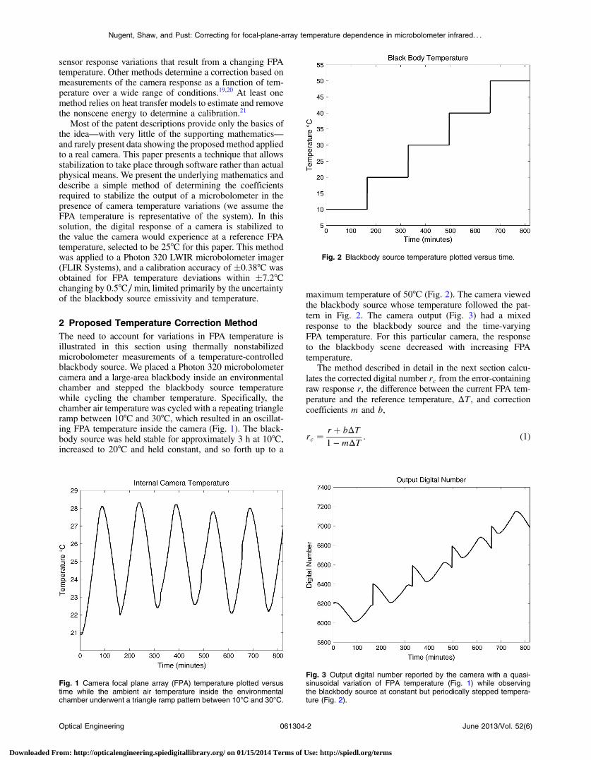
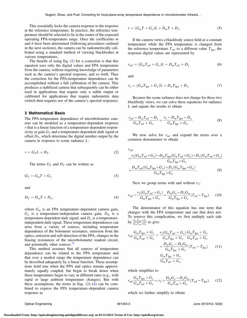
2 Proposed Temperature Correction MethodThe need to account for variations in FPA temperature isillustrated in this section using thermally nonstabilizedmicrobolometer measurements of a temperature-controlledblackbody source. We placed a Photon 320 microbolometercamera and a large-area blackbody inside an environmentalchamber and stepped the blackbody source temperaturewhile cycling the chamber temperature. Specifically, thechamber air temperature was cycled with a repeating triangleramp between 10°C and 30°C, which resulted in an oscillat-ing FPA temperature inside the camera (Fig. 1). The black-body source was held stable for approximately 3 h at 10°C,increased to 20°C and held constant, and so forth up to a

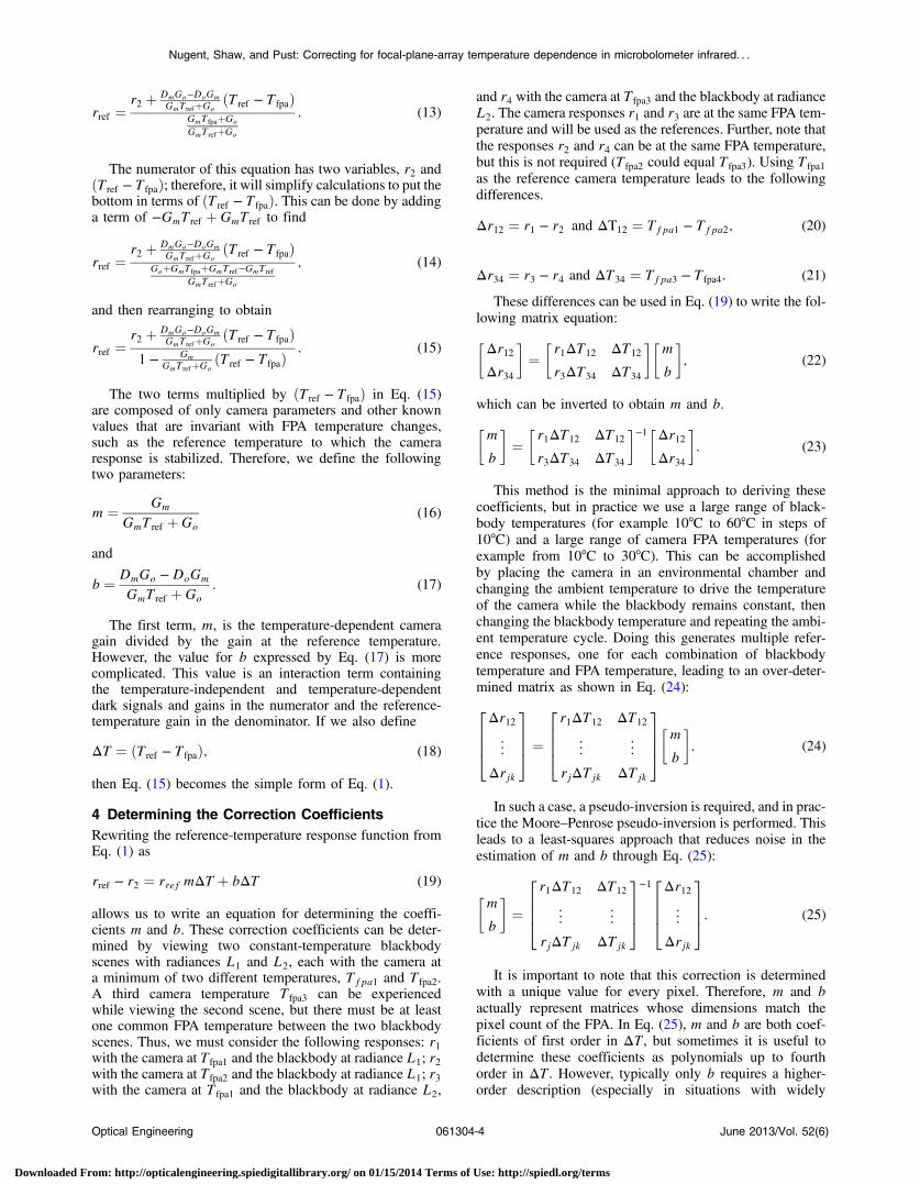
maximum temperature of 50°C (Fig. 2). The camera viewedthe blackbody source whose temperature followed the pat-tern in Fig. 2. The camera output (Fig. 3) had a mixedresponse to the blackbody source and the time-varyingFPA temperature. For this particular camera, the responseto the blackbody scene decreased with increasing FPAtemperature.

The method described in detail in the next section calcu-lates the corrected digital number rc from the error-containingraw response r, the difference between the current FPA tem-perature and the reference temperature, ΔT, and correctioncoefficients m and b,

rc ¼rþ bΔT1 −mΔT

: (1)

Fig. 1 Camera focal plane array (FPA) temperature plotted versustime while the ambient air temperature inside the environmentalchamber underwent a triangle ramp pattern between 10°C and 30°C.

Fig. 2 Blackbody source temperature plotted versus time.

Fig. 3 Output digital number reported by the camera with a quasi-sinusoidal variation of FPA temperature (Fig. 1) while observingthe blackbody source at constant but periodically stepped tempera-ture (Fig. 2).


Nugent, Shaw, and Pust: Correcting for focal-plane-array temperature dependence in microbolometer infrared. . .


This essentially locks the camera response to the responseat the reference temperature. In practice, the reference tem-perature should be selected to lie at the center of the expectedoperating FPA-temperature range. Once the coefficients mand b have been determined (following procedures outlinedin the next sections), the camera can be radiometrically cali-brated using a standard method of viewing blackbodies atvarious temperatures.

The benefit of using Eq. (1) for a correction is that thisequation uses only the digital values and FPA temperaturefrom the camera, without requiring knowledge of parameterssuch as the camera’s spectral response, and so forth. Thusthe correction for the FPA-temperature dependence can beaccomplished without a full calibration of the camera. Thisproduces a stabilized camera that subsequently can be eitherused in applications that require only a stable output orcalibrated for applications that require radiometric data(which then requires use of the camera’s spectral response).

3 Mathematical BasisThe FPA-temperature dependence of microbolometer cam-eras can be modeled as a temperature-dependent responser that is a linear function of a temperature-dependent respon-sivity or gain GT and a temperature-dependent dark signal oroffset DT , which determine the digital number output by thecamera in response to scene radiance L:

r ¼ GTLþDT: (2)

The terms GT and DT can be written as

GT ¼ GmT þ Go (3)

and

DT ¼ DmT þDo; (4)

where Gm is an FPA temperature–dependent camera gain,Go is a temperature-independent camera gain, Dm is atemperature-dependent dark signal, and Do is a temperature-independent dark signal. These temperature dependences canarise from a variety of sources, including temperaturedependence of the bolometer resistance, emission from theoptics, emission and self-detection of the FPA, changes in thebiasing resistances of the microbolometer readout circuit,and potentially other sources.15

This method assumes that all sources of temperaturedependence can be related to the FPA temperature andthat over a modest range the temperature dependence canbe described adequately by a linear function. These assump-tions hold true when the FPA and optics remain approxi-mately equally coupled, but begin to break down whenthese temperatures begin to vary at different rates (e.g., withrapid or large ambient temperature changes). But withthese assumptions, the terms in Eqs. (2)–(4) can be com-bined to express the FPA temperature–dependent cameraresponse as

r ¼ ðGmT þ GoÞLþDmT þDo: (5)

If the camera views a blackbody source held at a constanttemperature while the FPA temperature is changed fromthe reference temperature Tref to a different value Tfpa, theresponse digital values are represented by

rref ¼ ðGmTref þ GoÞLþDmTref þDo (6)

and

r2 ¼ ðGmTfpa þ GoÞLþDmTfpa þDo: (7)

Because the scene radiance does not change for these twoblackbody views, we can solve these equations for radianceL and equate the results to obtain

rref −DmTref −Do

GmTref þ Go¼ r2 −DmTfpa −Do

GmTfpa þGo: (8)

We now solve for rref and expand the terms over acommon denominator to obtain

rref

¼r2ðGmTrefþGoÞ−DmTfpaðGmTrefþGoÞ−DoðGmTrefþGoÞGmTfpaþGo

þDmTrefðGmTfpaþGoÞþDoðGmTfpaþGoÞGmTfpaþGo

: (9)

Next we group terms with and without r2:

rref ¼r2ðGmTrefþGoÞGmTfpaþGo

þDmGo−DoGm

GmTfpaþGoðTref −TfpaÞ: (10)

The denominator of this equation has one term thatchanges with the FPA temperature and one that does not.To remove this complication, we first multiply each sideby GmT fpaþGo

GmTrefþGoto give

rrefGmTfpa þ Go

GmTref þ Go¼ r2ðGmTref þ GoÞ

GmTfpa þ Go

GmTfpa þ Go

GmTref þ Go

þ DmGo −DoGm

GmTfpa þ GoðTref − TfpaÞ

GmTfpa þ Go

GmTref þGo;

(11)

which simplifies to

rrefGmTfpaþGo

GmTref þGo¼ r2þ

DmGo −DoGm

GmTref þGoðTref −TfpaÞ; (12)

which we further simplify to obtain




rref ¼r2 þ DmGo−DoGm

GmTrefþGoðTref − TfpaÞ

GmTfpaþGo

GmTrefþGo

: (13)

The numerator of this equation has two variables, r2 andðTref − TfpaÞ; therefore, it will simplify calculations to put thebottom in terms of ðTref − TfpaÞ. This can be done by addinga term of −GmTref þ GmTref to find



GoþGmTfpaþGmTref−GmTref

GmTrefþGo

; (14)

and then rearranging to obtain



1 − GmGmTrefþGo

ðTref − TfpaÞ: (15)

The two terms multiplied by ðTref − TfpaÞ in Eq. (15)are composed of only camera parameters and other knownvalues that are invariant with FPA temperature changes,such as the reference temperature to which the cameraresponse is stabilized. Therefore, we define the followingtwo parameters:

m ¼ Gm

GmTref þGo(16)

and

b ¼ DmGo −DoGm

GmTref þGo: (17)

The first term, m, is the temperature-dependent cameragain divided by the gain at the reference temperature.However, the value for b expressed by Eq. (17) is morecomplicated. This value is an interaction term containingthe temperature-independent and temperature-dependentdark signals and gains in the numerator and the reference-temperature gain in the denominator. If we also define

ΔT ¼ ðTref − TfpaÞ; (18)

then Eq. (15) becomes the simple form of Eq. (1).

4 Determining the Correction CoefficientsRewriting the reference-temperature response function fromEq. (1) as

rref − r2 ¼ rref mΔT þ bΔT (19)

allows us to write an equation for determining the coeffi-cients m and b. These correction coefficients can be deter-mined by viewing two constant-temperature blackbodyscenes with radiances L1 and L2, each with the camera ata minimum of two different temperatures, Tfpa1 and Tfpa2.A third camera temperature Tfpa3 can be experiencedwhile viewing the second scene, but there must be at leastone common FPA temperature between the two blackbodyscenes. Thus, we must consider the following responses: r1with the camera at Tfpa1 and the blackbody at radiance L1; r2with the camera at Tfpa2 and the blackbody at radiance L1; r3with the camera at Tfpa1 and the blackbody at radiance L2,

and r4 with the camera at Tfpa3 and the blackbody at radianceL2. The camera responses r1 and r3 are at the same FPA tem-perature and will be used as the references. Further, note thatthe responses r2 and r4 can be at the same FPA temperature,but this is not required (Tfpa2 could equal Tfpa3). Using Tfpa1

as the reference camera temperature leads to the followingdifferences.

Δr12 ¼ r1 − r2 and ΔT12 ¼ Tfpa1 − Tfpa2; (20)

Δr34 ¼ r3 − r4 and ΔT34 ¼ Tfpa3 − Tfpa4. (21)

These differences can be used in Eq. (19) to write the fol-lowing matrix equation:

�Δr12Δr34

�¼

�r1ΔT12 ΔT12

r3ΔT34 ΔT34

��m

b

�; (22)

which can be inverted to obtain m and b.

�m

b

�¼

�r1ΔT12 ΔT12

r3ΔT34 ΔT34

�−1�Δr12Δr34

�: (23)

This method is the minimal approach to deriving thesecoefficients, but in practice we use a large range of black-body temperatures (for example 10°C to 60°C in steps of10°C) and a large range of camera FPA temperatures (forexample from 10°C to 30°C). This can be accomplishedby placing the camera in an environmental chamber andchanging the ambient temperature to drive the temperatureof the camera while the blackbody remains constant, thenchanging the blackbody temperature and repeating the ambi-ent temperature cycle. Doing this generates multiple refer-ence responses, one for each combination of blackbodytemperature and FPA temperature, leading to an over-deter-mined matrix as shown in Eq. (24):

2664Δr12...

Δrjk

3775 ¼

2664r1ΔT12 ΔT12

..

. ...

rjΔTjk ΔTjk

3775�m

b

�. (24)

In such a case, a pseudo-inversion is required, and in prac-tice the Moore–Penrose pseudo-inversion is performed. Thisleads to a least-squares approach that reduces noise in theestimation of m and b through Eq. (25):

�m

b

�¼

2664r1ΔT12 ΔT12

..

. ...

rjΔTjk ΔTjk

3775−12664Δr12...

Δrjk

3775: (25)

It is important to note that this correction is determinedwith a unique value for every pixel. Therefore, m and bactually represent matrices whose dimensions match thepixel count of the FPA. In Eq. (25), m and b are both coef-ficients of first order in ΔT, but sometimes it is useful todetermine these coefficients as polynomials up to fourthorder in ΔT. However, typically only b requires a higher-order description (especially in situations with widely




ranging FPA temperature), whereas m can remain a first-order coefficient.

Also note that the absolute temperature or radiance of theblackbody source is not needed in this temperature-stabiliza-tion method, since the blackbody is only used as a stablereference. The only requirement is for the source to remainstable during the measurements at multiple FPA tempera-tures. The correction uses only the measured responses andthe camera FPA temperature, with no need for additionalinformation about the camera’s spectral response orthe blackbody source temperature (the camera spectralresponse is needed for the final radiometric calibration,but not for compensating for the FPA-temperature depend-ence). Nevertheless, performing this technique at two ormore blackbody temperatures improves the accuracy ofthe coefficients in the correction. This case generates multi-ple reference responses, one for each blackbody temperature,leading to an overdetermined matrix, thus reducing noise inthe estimation of m and b.

5 Application of the MethodThe procedure to use this method to determine a tempera-ture-stabilized radiometric calibration for a LWIR camerais presented in Fig. 4. First, the scene image and the FPAtemperature are measured concurrently. The temperature-dependent responsivity and offset coefficients m and b arethen used to stabilize the camera to its response at Tref .Finally, the stabilized response is calibrated by applying con-ventional gain and offset terms that were measured at orreferenced to Tref . These gain and offset values convertthe FPA temperature–stabilized data into values of integratedradiance seen by the detector. If needed, the radiance datacan be converted to temperature through a lookup table cre-ated by integrating the product of the blackbody function andthe camera’s spectral response function.

Calibrating the imager in units of integrated radiancerather than temperature has advantages, most notably thenominally linear response of photo detectors with radianceor other radiometric quantities proportional to photon irradi-ance. This in turn allows extrapolation to very low radiancevalues using a calibration performed with measurements ofmuch warmer blackbody sources.13,22,23 Although ourtechnique calibrates to radiance, techniques that calibratedirectly to temperature could also use the FPA temperature–stabilized data (calibrating directly in temperature requires

compensating for the nonlinear relationship between thetemperature of an object and its emitted radiance24).

As an example of successful implementation on a micro-bolometer camera without thermal stabilization, we appliedthis method to a FLIR Photon 320 camera with a 14.25-mmlens. The camera was placed with a large-area blackbodyinside an environmental chamber. Throughout the experi-ment, the blackbody filled the 50 deg- by 38-deg camerafield of view. The blackbody was an Electro-OpticalIndustries CES-100 with a 15-cm aperture and microgroovesurface specified with a 0.995 emissivity. The blackbody wasfactory calibrated with a NIST-traceable temperature uncer-tainty of 0.1°C. Background radiance reflected from theblackbody was removed from blackbody measurements,but was typically less than 0.75% of the observed blackbodyradiance.

In this experiment, blackbody images were acquired asthe source temperature was increased from 10°C to 60°C

Fig. 4 Flow diagram for stabilization and radiometric calibration usingonly the FPA temperature.

Fig. 5 Camera FPA temperature (solid line) and blackbody sourcetemperature (dashed line) during a 24-h experiment to validate thecamera stabilization method.

Fig. 6 Uncorrected (black) and corrected (red) digital numbers outputfrom a microbolometer camera with a variable FPA temperature. Solidlines indicate the spatial mean across the FPA, and dashed linesindicate the maximum and minimum values across the FPA.




in steps of 16.7°C every 6 h. While the blackbody washeld constant at each setting, the ambient temperatureof the chamber was ramped in a triangle wave patternbetween 15°C and 30°C in steps of 1°C every 5 min.These images were used to derive matrices of m and b coef-ficients for the stabilization Eq. (1) with biðΔTÞi terms up toorder i ¼ 3

The uncertainty in the resulting calibration was deter-mined by placing the camera back inside the chamber andacquiring calibrated images of the blackbody source atdifferent temperatures. The chamber air temperature was var-ied to match the outdoor air temperature measured by ourweather station on a summer day and night in Bozeman, MT(ranging between 13.9°C and 26.4°C). The blackbody tem-perature was stepped between 10°C and 50°C and held con-stant for a variable length of time. The FPA temperatures andblackbody temperatures during this experiment are shown inFig. 5. The measured data before FPA-temperature correc-tion (black) and after correction (red) are shown in Fig. 6.Solid lines indicate the spatial mean across the FPA,while dashed lines indicate the maximum and minimum val-ues at each instant of time (the spatial standard deviationswere indistinguishably close to the mean line).

With the camera’s response stabilized as shown in Fig. 6,a conventional two-point radiometric calibration was appliedusing blackbody temperatures of 10°C and 60°C. Figure 7 isa time-series plot of the calibrated camera output and theblackbody source temperature for the 24-h experiment justdescribed. The solid line indicates the spatial mean acrossthe FPA, whereas the dashed lines indicate the maximum andminimum values across the FPA at each instant of time (thespatial standard deviations again were indistinguishablyclose to the mean line).

Figure 8 is a time-series plot of the difference between theblackbody source temperature and the temperature reportedby the camera (from the calibrated radiance). The dashedlines in this figure indicate the expected blackbody-relatedcalibration uncertainty of �0.32°C. This value arises fromcombining the blackbody temperature uncertainty (�0.1°C)and the blackbody emissivity uncertainty (0.995� 0.005)in the two-point calibration.25 The blackbody temperatureuncertainty includes blackbody spatial variation and uncer-tainties in readout, temperature sensor calibration, and tem-poral variation. The effect of the emissivity uncertainty on

Fig. 7 Calibrated temperature readings averaged across the FPA(red solid), maximum and minimum temperature readings acrossthe FPA (red dashed lines), and blackbody set temperatures (blackdashed line).

Fig. 8 Difference between the calibrated camera data and the black-body set points (red, rms variability ¼ 0.21°C), along with the 0.32°Cblackbody-related uncertainty (dashed black). The dashed gray linesindicate the maximum and minimum differences in each frame.

Fig. 9 The histogram of the error of 300 randomly selected data files calibrated without FPA temperature compensation (a) and with FPA temper-ature compensation (b).




the calibration depends on the ambient temperature rangeexperienced in the experiment.

Figure 8 shows that the difference of the measurementsfrom the blackbody set-point temperatures was within theexpected uncertainty for nearly all readings. The spatialrms variation of the difference varied over time, with typicalvalues of 0.08°C and a maximum value of 0.19°C. The tem-poral rms variation of this difference was 0.09°C, leading to atotal spatial-temporal variability of 0.21°C. The maximumsustained difference was 0.75°C, which occurred between300 and 450 min after the experiment began. The maximuminstantaneous error wasþ1.98°C in a single observation near1150 min. However, this and other single-frame errors arebelieved to be blinking of residual bad pixels.

Figure 9 shows two histograms that provide a final illus-tration of the significance of this camera stabilizationmethod, using 300 frames chosen at random times fromthe 24-h measurement sequence on which Figs. 5–8 arebased. The histogram in Fig. 9(a) shows the distribution ofmeasurement errors relative to the blackbody set point with-out camera stabilization, and Fig. 9(b) shows the distributionof errors with stabilization. The errors are spread over�6.25°C without stabilization and�0.3°C with stabilization.It is also interesting to note that stabilization converts therelatively uniform error distribution in Fig. 9(a) to aGaussian-like distribution in Fig. 9(b).

During these validation experiments, the flat field correc-tion (FFC) of the camera was manually controlled to happenevery 5 min or 0.4°C change in FPA temperature. By study-ing images collected before and after the FFC, it was foundthat the FFC had only a minor impact on the stabilized cam-era calibration. Just after an FFC is done, the reported tem-perature changed by an amount between 0.1°C and 0.25°C,decreasing when the FPA temperature was decreasing andincreasing when the FPA temperature was increasing.

6 Discussion and ConclusionThis method allows for correction of the FPA temperature-de-pendent errors in the response of microbolometer cameras. It isunique from previously reported techniques in that it allows thestabilization to take place without a full radiometric calibrationof the camera, and without requiring specific informationabout the camera that would be required in other techniques.In operation, the output data from the imager can be adjustedfor the FPA temperature-induced errors, thus stabilizing theresponse of otherwise highly temperature-dependent cameras.Radiometric calibration and other data processing then can beperformed on the stabilized camera response.

In many thermal infrared imaging applications, use of thetechnique described here can eliminate costly and space-intensive blackbody sources in field-deployed instruments,provide radiometric calibration of otherwise uncalibratedcameras, and improve the stability and accuracy of datafrom thermal imagers. For example, the reported techniquebenefits any application in which a radiometrically calibratedthermal camera is required and wherein the cost, space, orweight of an external blackbody is not desired or practical.

The reported technique was carefully implemented on aFLIR Photon 320 camera, producing a calibration with rmsvariability of 0.21°C, total calibration uncertainty of 0.38°C,and a maximum error of 0.75°C in a 24-h period. This cal-ibration uncertainty is better than the value of�2°C specified

for most commercial microbolometer imagers. The primarycontributors to the calibration uncertainty are blackbodysource emissivity and temperature. This process has pro-duced similar results on a variety of FLIR cameras, includingthe Photon 320 with several wide and narrow lenses,PathFindIR, Photon 640, Tau 320, and Tau 640.

References

1. P. W. Kruse, Uncooled Thermal Imaging, Arrays, Systems, andApplications, p. 64, SPIE, Bellingham, WA (2002).

2. F. Niklaus, C. Vieider, and H. Jakobsen, “MEMS-based uncooled infra-red bolometer arrays: a review,” Proc. SPIE 6836, 68360D (2007).

3. R. K. Bhan et al., “Uncooled infrared microbolometer arrays and theircharacterisation techniques,” Defence Sci. J. 59(6), 580–589 (2009).

4. S. Garcia-Blanco et al., “Radiometric packaging of uncooled microbolom-eter FPA arrays for space applications,” Proc. SPIE 7206, 720604 (2009).

5. H. Geoffray et al., “Evaluation of a COTS microbolometers FPA tospace environments,” Proc. SPIE 7826, 78261U (2010).

6. R. Vadivambal and D. S. Jayas, “Applications of thermal imaging inagriculture and food industry: a review,” Food Bioprocess. Technol.4(2), 186–199 (2011).

7. S. Rayne and G. S. Henderson, “Airborne thermal infrared remote sens-ing of stream and riparian temperatures in the Nicola River watershed,British Columbia, Canada,” J. Environ. Hydrol. 12, 1–11 (2004).

8. D. A. Socolinsky, A. Selinger, and J. D. Neuheisel, “Face recognitionwith visible and thermal infrared imagery,” Comp. Vis. ImageUnderstand. 91(1–2), 72–114 (2003).

9. J. A. Shaw et al., “Long-wave infrared imaging for non-invasive beehivepopulation assessment,” Opt. Express 19(1), 399–408 (2011).

10. J. E. Johnson et al., “Long-wave infrared imaging of vegetation fordetecting leaking CO2 gas,” J. Appl. Rem. Sens. 6(1), 063612 (2012).

11. M. Vollmer and K.-P. Möllmann, Infrared Thermal Imaging, Wiley-VCH, Weinheim, Germany (2010).

12. M. W. Kudenov, J. L. Pezzaniti, and G. R. Gerhart, “Microbolometer-infrared imaging Stokes polarimeter,” Opt. Eng. 48(6), 063201 (2009).

13. J. Shaw et al., “Radiometric cloud imaging with an uncooled microbolom-eter thermal infrared camera,” Opt. Express 13(15), 5807–5817 (2005).

14. P. W. Nugent, J. A. Shaw, and S. Piazzolla, “Infrared cloud imaging insupport of Earth-space optical communication,” Opt. Express 17(10),7862–7872 (2009).

15. T. Hoelter and B. Meyer, “The challenges of using an uncooled micro-bolometer array in a thermographic application,” 1998, http://www.dtic.mil/cgi-bin/GetTRDoc?Location=U2&doc=GetTRDoc.pdf&AD=ADA399432 (28 September 2012).

16. M. A. Wand et al., “Ambient temperature micro-bolometer control,calibration, and operation,” U.S. Patent 6267501 (2001).

17. S. M. Anderson and T. McManus, “Microbolometer focal plane arraywith temperature compensated bias,” U.S. Patent 7105818 (2006).

18. N. R. Butler, “Method and apparatus for compensating radiation sensorfor temperature variations of the sensor,” U.S. Patent 6740909 (2004).

19. P. E. Howard, “Infrared sensor temperature compensated response andoffset correction,” U.S. Patent 6433333 (2002).

20. C. S. Kaufman, R. S. Carson, and W. B. Hornback, “Method and appa-ratus for temperature compensation of an uncooled focal plane array,”U.S. Patent 6476292 (2002).

21. E. Grimberg, “Radiometry using an uncooled microbolometer detector,”U.S. Patent application US2008/0210872 (2008).

22. Y. Han et al., “Infrared spectral radiance measurements in the tropicalPacific atmosphere,” J. Geophys. Res. 102(D4), 4353–4356 (1997).

23. R. O. Knuteson et al., “Atmospheric emitted radiance interferometer.Part II: instrument performance,” J. Atmos. Ocean. Technol. 21(12),1777–1789 (2004).

24. J. A. Shaw and L. S. Fedor, “Improved calibration of infrared radiom-eters for cloud temperature remote sensing,” Opt. Eng. 32(5),1002–1010 (1993).

25. C. L. Wyatt, V. Privalsky, and R. Datla, “Recommended practice;symbols, terms, units and uncertainty analysis for radiometric sensorcalibration,” in NIST Handbook 152, U.S. Government PrintingOffice, Washington, DC (1998).

Paul W. Nugent is a research engineer withthe Electrical and Computer EngineeringDepartment at Montana State Universityand president of NWB Sensors Inc. inBozeman, Montana. He received his MSand BS degrees in electrical engineeringfrom Montana State University. His researchactivities include radiometric thermal imagingand optical remote sensing.




http://dx.doi.org/10.1117/12.755128

http://dx.doi.org/10.1117/12.810025

http://dx.doi.org/10.1117/12.869726

http://dx.doi.org/10.1007/s11947-010-0333-5

http://dx.doi.org/10.1016/S1077-3142(03)00075-4

http://dx.doi.org/10.1016/S1077-3142(03)00075-4

http://dx.doi.org/10.1364/OE.19.000399

http://dx.doi.org/10.1117/1.JRS.6.063612

http://dx.doi.org/10.1117/1.3156844

http://dx.doi.org/10.1364/OPEX.13.005807

http://dx.doi.org/10.1364/OE.17.007862

http://www.dtic.mil/cgi-bin/GetTRDoc?Location=U2&doc=GetTRDoc.pdf&AD=ADA399432





http://dx.doi.org/10.1029/96JD03717

http://dx.doi.org/10.1175/JTECH-1663.1

http://dx.doi.org/10.1117/12.133232

Joseph A. Shaw is the director of the OpticalTechnology Center, professor of electricaland computer engineering, and affiliateprofessor of physics at Montana StateUniversity in Bozeman, Montana. Hereceived PhD and MS degrees in opticalsciences from the University of Arizona, anMS degree in electrical engineering fromthe University of Utah, and a BS degree inelectrical engineering from the University ofAlaska–Fairbanks. He conducts research

on the development and application of radiometric, polarimetric,and laser-based optical remote sensing systems. He is a Fellow ofthe OSA and SPIE.

Nathan J. Pust is a research engineer work-ing at Montana State University. He receivedbachelor’s degrees in electrical engineeringand computer engineering from MontanaState University in 2002, and his PhD inelectrical engineering from Montana StateUniversity in 2007.




correcting for focal-plane-array temperature dependence in ... fpa temp... · correcting for...

Documents