FEDERAL RESERVE BANK OF SAN FRANCISCO

WORKING PAPER SERIES

Correcting Estimation Bias in Dynamic Term Structure Models

Michael D. Bauer

Federal Reserve Bank of San Francisco

Glenn D. Rudebusch Federal Reserve Bank of San Francisco

Jing (Cynthia) Wu

Booth School of Business, University of Chicago

April 2012

Working Paper 2011-12 http://www.frbsf.org/publications/economics/papers/2011/wp11-12bk.pdf

The views in this paper are solely the responsibility of the authors and should not be interpreted as reflecting the views of the Federal Reserve Bank of San Francisco or the Board of Governors of the Federal Reserve System.

Correcting Estimation Bias in

Dynamic Term Structure Models∗

Michael D. Bauer†, Glenn D. Rudebusch‡, Jing Cynthia Wu§

First version: April 4, 2011

This draft: April 2, 2012

Abstract

The affine dynamic term structure model (DTSM) is the canonical empirical finance

representation of the yield curve. However, the possibility that DTSM estimates may be

distorted by small-sample bias has been largely ignored. We show that conventional esti-

mates of DTSM coefficients are indeed severely biased, and this bias results in misleading

estimates of expected future short-term interest rates and of long-maturity term premia.

We provide a variety of bias-corrected estimates of affine DTSMs, both for maximally-

flexible and over-identified specifications. Our estimates imply short rate expectations

and term premia that are more plausible from a macro-finance perspective.

Keywords: small-sample bias correction, vector autoregression, dynamic term structure

models, term premium

JEL Classifications: C53, E43, E47

∗We thank Jim Hamilton, Chris Hansen, Oscar Jorda, Lutz Kilian, and Jonathan Wright for their helpfulcomments, as well as participants of research seminars at the Federal Reserve Bank of San Francisco andUC San Diego, and of the Econometric Society 2011 Winter Meetings, the European Economic Association2011 Conference, the Society for Computational Economics 2011 Conference, and the Society of FinancialEconometrics 2011 Conference. The views in this paper do not necessarily reflect those of others in theFederal Reserve System.

†Federal Reserve Bank of San Francisco, michael.bauer@sf.frb.org‡Federal Reserve Bank of San Francisco, glenn.rudebusch@sf.frb.org§Booth School of Business, University of Chicago, cynthia.wu@chicagobooth.edu

1 Introduction

The affine Gaussian dynamic term structure model (DTSM) is the canonical empirical finance

representation of the yield curve, used to study a variety of questions about the interactions

of asset prices, risk premia, and economic variables. One question of fundamental importance

to both researchers and policymakers is to what extent movements in long-term interest rates

reflect changes in expected future policy rates or changes in term premia. The answer to

this question depends on the estimated dynamic system for the risk factors underlying yields,

which in affine DTSMs is specified as a vector autoregression (VAR). Because of the high

persistence of interest rates, maximum likelihood (ML) estimates of such models likely suffer

from serious small-sample bias. Namely, interest rates will be spuriously estimated to be less

persistent than they really are. While this problem has been recognized in the literature,

no study to date has attempted to obtain bias-corrected estimates of a DTSM, quantify the

extent of estimation bias, or assess the implications of that bias for economic inference. In

this paper we provide a readily applicable methodology for bias-corrected estimation of both

maximally-flexible (exactly identified) and restricted (over-identified) affine DTSMs. Our

estimates uncover significant bias in standard DTSM coefficient estimates and show that

accounting for this bias substantially alters economic conclusions.

The bias in ML estimates of the VAR parameters in an affine DTSM parallels the well-

known bias in ordinary least squares (OLS) estimates of autoregressive systems. Such esti-

mates will generally be biased toward a dynamic system that displays less persistence than

the true process. This bias is particularly severe when the estimation sample is short and

the dynamic process is very persistent. Empirical DTSMs are invariably estimated under just

such conditions, with data samples that contain only a limited number of interest rate cycles.

Hence, the degree of interest rate persistence is likely to be seriously underestimated. Conse-

quently, expected future short rates will appear to revert too quickly to their unconditional

mean, resulting in spuriously stable estimates of risk-neutral rates. Furthermore, the estima-

tion bias that contaminates readings on expected future short rates also distorts estimates of

long-maturity term premia.

While the qualitative implications of the small-sample DTSM estimation bias are quite

intuitive, the magnitude of the bias and its impact on inference about expected short-rate

paths and risk premia have been unclear. The ML methods typically used to estimate DTSMs

were intensive, “hands-on” procedures because these models exhibited relatively flat likeli-

hood surfaces with many local optima.1 The computational burden of estimation effectively

1Studies that describe these problems include Hamilton and Wu (2010) and Christensen et al. (2011).

1

precluded the application of simulation-based bias correction methods. However, recent work

by Joslin et al. (2011) (henceforth JSZ) and Hamilton and Wu (2010) (henceforth HW) has

shown that OLS can be used to solve part of the estimation problem. We exploit these new

procedures to facilitate bias-corrected estimation of DTSMs through repeated simulation and

estimation. Specifically, we adapt the two-step estimation approaches of JSZ and HW by

replacing the OLS estimates of the autoregressive system in the first step by simulation-based

bias-corrected estimates. We then proceed with the second step of the estimation, which re-

covers the parameters determining the cross-sectional fit of the model, in the usual way. This

new estimation approach is a key methodological innovation of the paper.

There are several different existing approaches to correct for small-sample bias in estimates

of a VAR, including analytical bias approximations and bootstrap bias correction. While each

of these could be applied to our present context, we favor our own novel bias correction pro-

cedure for VAR estimation: Our “inverse bootstrap” bias correction finds the data-generating

process (DGP) parameters that lead to a mean or median of the OLS estimator equal to

the original OLS estimates. While this approach is not conceptually novel—it is closely re-

lated to indirect inference (Gourieroux et al., 2000) and to the median-unbiased estimators

of Andrews (1993) and Rudebusch (1992)—we provide a new algorithm, based on results

from the stochastic approximation literature, that allows us to quickly and reliably calculate

bias-corrected estimators.

We first apply our methodology for bias-corrected DTSM estimation to the maximally-

flexible DTSM that was estimated in JSZ. In this setting, the ML estimates of the VAR

parameters are exactly recovered by OLS. Using the authors’ same model specifications and

data samples, we quantify the bias in the reported parameter estimates and describe the

differences in the empirical results when the parameters governing the factor dynamics are

replaced with bias-corrected estimates. We find a very large estimation bias in JSZ. That is,

the conventional estimates of JSZ imply a severe overestimation of the speed of interest rate

mean reversion. As a result, the decomposition of long-term interest rates into expectations

and risk premium components differs in statistically and economically significant ways between

conventional ML and bias-corrected estimates. Risk-neutral forward rates, i.e., short-rate

expectations, are substantially more volatile after correction for estimation bias, and they show

a pronounced decrease over the last twenty years, consistent with lower longer-run inflation

and interest rate expectations documented in the literature (Kozicki and Tinsley, 2001; Kim

and Orphanides, 2005; Wright, 2011). Furthermore, bias correction leads to term premia

that are elevated around recessions and subdued during expansions, consistent with much

theoretical and empirical research that supports countercyclical risk compensation.

2

In our second empirical application, we estimate a DTSM with overidentifying restrictions.

HW show that any affine DTSM—maximally-flexible or overidentified—can be estimated by

first obtaining reduced-form parameters using OLS and then calculating all structural parame-

ters via minimum-chi-squared estimation. Many estimated DTSMs impose parameter restric-

tions to avoid overfitting and to facilitate numerical optimization of the likelihood function

(examples include Ang and Piazzesi, 2003; Kim and Wright, 2005; Joslin et al., 2010). Re-

strictions on risk pricing (Cochrane and Piazzesi, 2008; Bauer, 2011b; Joslin et al., 2010) have

an additional benefit: They exploit the no-arbitrage condition, which ties the cross-sectional

behavior of interest rates to their dynamic evolution, to help pin down the estimates of the

parameters of the dynamic system. In this way, such restrictions could potentially reduce the

bias in the estimates of these parameters. However, we find that the bias in ML estimates of

a DTSM with risk price restrictions is large, indeed, similar in magnitude to our results for

the maximally-flexible model. While this result may not generalize to all restricted models,

it shows that simply zeroing out some risk price parameters will not necessarily eliminate

estimation bias.

There are a number of papers in the literature that are related to ours. Several studies

attempt to indirectly reduce the bias in DTSM estimates—using risk price restrictions (see

above), survey data (Kim and Orphanides, 2005; Kim and Wright, 2005), or near-cointegrated

VAR specifications (Jardet et al., 2011)—but do not quantify the bias nor provide evidence

as to how much it is reduced. Another group of papers has performed simulation studies to

show the magnitude of the bias in DTSM estimates relative to some stipulated DGP (Ball

and Torous, 1996; Duffee and Stanton, 2004; Kim and Orphanides, 2005). These studies

demonstrate that small-sample bias can be an issue using simulation studies, but do not

quantify its magnitude or assess its implications for models estimated on real data. The most

closely related paper Phillips and Yu (2009), which also performs bias-corrected estimation

of asset pricing models. That analysis parallels ours in that the authors also use simulation-

based bias correction and show the economic implications of correcting for small-sample bias.

However, their focus differs from ours in that they aim at reducing the bias in prices of

contingent claims, whereas we address a different economic question, namely the implications

of small-sample bias on estimated policy expectations and nominal term premia.

Our paper is structured as follows: Section 2 describes the model, the econometric problems

with conventional estimation, and the intuition of our methodology for bias-corrected estima-

tion. In Section 3, we discuss OLS estimates of interest rate VARs and the improvements

from bias-corrected estimates. In Section 4, we describe how to estimate maximally-flexible

models with bias correction, apply this methodology to the model of JSZ, and discuss the

3

statistical and economic implications. We also perform a simulation study to systematically

assess the value of bias correction in such a context. In Section 5, we show how to perform

bias-corrected estimation for restricted models, adapting the methodology of HW, and apply

this approach to a model with restrictions on the risk pricing. Section 6 concludes.

2 Estimation of affine models

In this section, we set up a standard affine Gaussian DTSM, and describe the econometric

issues, including small-sample bias, that arise due to the persistence of interest rates. Then

we discuss recent methodological advances and how they make bias correction feasible.

2.1 Model specification

The discrete-time affine Gaussian DTSM, the workhorse model in the term structure literature

since Ang and Piazzesi (2003), has three key elements. First, a vector of N risk factors, Xt,

follows a first-order Gaussian VAR under the objective probability measure P:

Xt+1 = µ+ ΦXt + Σεt+1, (1)

where εtiid∼ N(0, IN) and Σ is lower triangular. Time t is measured in months throughout the

paper. Second, the short rate, rt, is an affine function of the pricing factors:

rt = δ0 + δ′1Xt. (2)

Third, the stochastic discount factor (SDF) that prices all assets under the absence of arbitrage

is of the essentially affine form (Duffee, 2002):

− log(Mt+1) = rt +1

2λ′

tλt + λ′

tεt+1,

where the N -dimensional vector of risk prices is affine in the pricing factors,

λt = λ0 + λ1Xt,

for N -vector λ0 and N ×N matrix λ1. As a consequence of these assumptions, a risk-neutral

probability measure Q exists such that the price of an m-period default-free zero coupon bond

4

is Pmt = E

Qt (e

−∑

m−1

h=0rt+h), and under Q the risk factors also follow a Gaussian VAR,

Xt+1 = µQ + ΦQXt + ΣεQt+1. (3)

The prices of risk determine how the change of measure affects the VAR parameters:

µQ = µ− Σλ0 ΦQ = Φ− Σλ1. (4)

Bond prices are exponentially affine functions of the pricing factors:

Pmt = eAm+B′

mXt ,

with loadings Am = Am(µQ,ΦQ, δ0, δ1,Σ) and Bm = Bm(Φ

Q, δ1) that follow the recursions

Am+1 = Am + (µQ)′Bm +1

2B′

mΣΣ′Bm − δ0

Bm+1 = (ΦQ)′Bm − δ1

with starting values A0 = 0 and B0 = 0. Model-implied yields are ymt = −m−1 logPmt =

Am + B′mXt, with Am = −m−1Am and Bm = −m−1Bm. Risk-neutral yields, the yields that

would prevail if investors were risk-neutral, can be calculated using

ymt = Am + B′

mXt, Am = −m−1Am(µ,Φ, δ0, δ1,Σ), Bm = −m−1Bm(Φ, δ1).

Risk-neutral yields reflect policy expectations over the lifetime of the bond, m−1∑m−1

h=0 Etrt+h,

plus a time-constant convexity term. The yield term premium is defined as the difference

between actual and risk-neutral yields, ytpmt = ymt − ymt . Model-implied forward rates for loans

starting at t + n and maturing at t + m are given by fn,mt = (m − n)−1(logP n

t − logPmt ) =

(m − n)−1(mymt − nynt ). Risk-neutral forward rates fn,mt are calculated in analogous fashion

from risk-neutral yields. The forward term premium is defined as ftpn,mt = fn,mt − f

n,mt .

The appeal of a DTSM is that all yields, forward rates, and risk premia are functions of a

small number of risk factors. Let M be the number of yields in the data used for estimation.

The M-vector of model-implied yields is Yt = A + BXt, with A = (Am1, . . . , AmM

)′ and

B = (Bm1, . . . , BmM

)′. A low-dimensional model will not have perfect empirical fit for all

yields, so we specify observed yields to include a measurement error, Yt = Yt + et. While

measurement error can potentially have serial correlation (Adrian et al., 2012; Hamilton and

Wu, 2011), we follow much of the literature and take et to be an i.i.d. process.

As in JSZ and HW we assume that N linear combinations of yields are priced without error.

5

Specifically, we take the first three principal components of yields as risk factors. Denote by W

the 3×M matrix that contains the eigenvectors corresponding to the three largest eigenvalues

of the covariance matrix of Yt. By assumption, Xt = WYt = WYt.2 Generally, risk factors

can be unobserved factors (which are filtered from observed variables), observables such as

yields or macroeconomic variables, or any combination of unobserved and observable factors.

Our estimation method is applicable to cases with observable and/or unobservable yield curve

factors, as well as to macro-finance DTSMs (Ang and Piazzesi, 2003; Rudebusch and Wu, 2008;

Joslin et al., 2010). The only assumption that is necessary for our method to be applicable is

that N linear combinations of risk factors are priced without error.

One possible parameterization of the model is in terms of γ = (µ,Φ, µQ,ΦQ, δ0, δ1,Σ),

leaving aside the parameters determining the measurement error distribution. Given γ, the

risk sensitivity parameters λ0 and λ1 follow from equation (4). Model identification requires

normalizing restrictions (Dai and Singleton, 2000). For example, γ has 34 free elements in a

three-factor model, but only 22 parameters are identified, so at least 12 normalizing restrictions

are necessary. If the model is exactly identified, one speaks of a “maximally-flexible” model,

as opposed to an over-identified model, in which additional restrictions are imposed.

2.2 Maximum likelihood estimation and small-sample bias

While it is conceptually straightforward to calculate the ML estimator (MLE) of γ, this has

been found to be very difficult in practice.3 The first issue is to numerically find the MLE,

which is problematic since the likelihood function is high-dimensional, badly behaved, and

typically exhibits local optima (with different economic implications). The second issue is

the considerable statistical uncertainty around the point estimates of DTSM parameters (Kim

and Orphanides, 2005; Rudebusch, 2007; Bauer, 2011b). The third issue, which is the focus

of this paper, is that the MLE suffers from small-sample bias (Ball and Torous, 1996; Duffee

and Stanton, 2004; Kim and Orphanides, 2005). All three of these problems are related to the

high persistence of interest rates, which complicates the inference about the VAR parameters.

Intuitively, because interest rates revert to their unconditional mean very slowly, a data sample

will typically contain only very few interest rate cycles, which makes it difficult to infer µ and Φ.

The likelihood surface is rather flat in certain dimensions around its maximum, thus numerical

optimization is difficult and statistical uncertainty is high. Furthermore, the severity of the

2Note that our principal components are not demeaned, and hence µ is not assumed to be zero.3The list of studies that have documented such problems is long and includes Ang and Piazzesi (2003);

Duffee and Stanton (2004); Kim and Orphanides (2005); Duffee (2011a) and Hamilton and Wu (2010). Also seeChristensen et al. (2009) and Christensen et al. (2011), who introduce an arbitrage-free Nelson-Siegel DTSMthat can be readily estimated.

6

small-sample bias depends positively on the persistence of process.

The economic implications of small-sample bias are likely to be important, because the

VAR parameters determine the risk-neutral rates and term premia. Since the bias causes the

speed of mean reversion to be overestimated, model-implied short-rate forecasts will tend to

be too close to their unconditional mean, especially at long horizons. Therefore, risk-neutral

rates will be too stable, and too large a portion of the movements in nominal interest rates

will be attributed to movements in term premia.

2.3 Bias correction for DTSMs

Simulation-based bias correction methods require repeated sampling of new data sets and

calculation of the estimator. For this to be computationally feasible, the estimator needs to

be calculated quickly and reliably for each simulated data set. In the DTSM context, MLE

has typically involved high computational cost, with low reliability in terms of finding a global

optimum, which effectively precluded simulation-based bias correction.

However, two important recent advances in the DTSM literature substantially simplify

estimation of affine Gaussian DTSMs. First, JSZ prove that in a maximally-flexible model the

MLE of µ and Φ can be obtained using OLS. Second, HW show that any affine Gaussian model

can be estimated by first estimating a reduced form of the model by OLS and then finding the

structural parameters by minimizing a chi-squared statistic. Given these methodological inno-

vations, there is no need to maximize a high-dimensional, badly behaved likelihood function.

Estimation can be performed by a consistent and efficient two-stage estimation procedure,

where the first stage consists of OLS, and the second stage involves finding the remaining

(JSZ) or structural (HW) parameters, without minimal computational difficulties.

These methodological innovations make correction for small-sample bias feasible, because

of their use of linear regressions to solve part of the estimation problem. In both approaches, a

VAR system is estimated in the first stage, which is the place where bias correction is needed.

We propose to apply bias correction techniques to the estimation of the VAR parameters, and

to carry out the rest of the estimation procedure in the normal fashion. This, in a nutshell, is

the methodology that we will use in this paper.

Before detailing our approach in Sections 4 (for maximally-flexible models) and 5 (for over-

identified models), we first discuss how to obtain bias-corrected estimates of VAR parameters,

as well as the particular features of the VARs in term structure models.

7

3 Bias correction for interest rate VARs

This section describes interest rate VARs, i.e., VARs that include interest rates or factors

derived from interest rates, and discusses small-sample OLS bias and bias correction in this

context.

3.1 Characteristic features of interest rate VARs

The factors in a DTSM include either individual interest rates, linear combinations of these,

or latent factors that are filtered from the yield curve, and hence will typically have similar

statistical properties as individual interest rates. The amount of persistence displayed by

both nominal and real interest rates is extraordinarily high (see, for example, Rose, 1988;

Goodfriend, 1991; Rapach and Weber, 2004). That is, first order autocorrelation coefficients

are typically close to one, and unit root tests often do not reject the null of a stochastic trend.

However, economic arguments strongly suggest that interest rates are stationary: A unit root

is implausible, since nominal interest rates generally do not turn negative and remain within

some limited range, and an explosive root (exceeding one) is unreasonable since forecasts

would diverge. For these reasons, empirical DTSMs almost invariably assume stationarity by

implicitly or explicitly imposing the constraint that all roots of the factor VAR are less than

one in absolute value.4 We assume that interest rates are stationary but potentiallly with a

very slow speed of mean reversion.

The data samples used in estimation of interest rate VARs are typically rather short.

Researchers often start their samples in the 80s or later because of data availability or potential

structural breaks (e.g., Joslin et al., 2010, 2011; Wright, 2011). Even if one goes back to the 60s

(e.g., Cochrane and Piazzesi, 2005; Duffee, 2011b), the sample can be considered rather short

in light of the high persistence of interest rates—there are only few interest rate cycles, and

uncertainty around the VAR parameters remains high. Notably, it does not matter whether

one samples at quarterly, monthly, weekly or daily frequency: sampling at a higher frequency

increases the sample length but also the persistence (Pierse and Snell, 1995).

Researchers attempting to estimate DTSMs are thus invariably faced with highly persistent

risk factors and short available data samples to infer the dynamic properties of the model.

4The stationarity prior is made explicit in the Bayesian frameworks of Ang et al. (2009) and Bauer (2011b).

8

3.2 Small-sample bias of OLS

Consider the VAR system in equation (1). We focus our exposition on a first-order VAR

since the extension to higher order models is straightforward. We assume that the VAR is

stationary, i.e., all the eigenvalues of Φ are less than one in modulus. The parameters of

interest are θ = vec(Φ). Denote the true values by θ0. The MLE of θ can be obtained by

applying OLS to each equation of the system (Hamilton, 1994, chap. 11.1). Let θT denote the

OLS estimator, and θ the estimates from a particular sample.

Because of the presence of lagged endogenous variables, the assumption of strict exogeneity

is violated, and the OLS estimator is biased in finite samples, i.e., E(θT ) 6= θ0. The bias

function bT (θ) = E(θT ) − θ relates the bias of the OLS estimator to the value of the data-

generating θ.5 The bias in θT is more severe the shorter the available sample and the more

persistent the process is (see, for example, Nicholls and Pope, 1988). Hence, for interest

rate VARs the bias is potentially sizeable. The consequence is that OLS underestimates the

persistence of the system, as measured for example by the largest eigenvalue of Φ or by the

half-life of shocks. Therefore, forecasts revert to the unconditional mean too quickly.

An alternative for defining bias is to consider the median as the relevant central tendency

of an estimator. Some authors, including Andrews (1993) and Rudebusch (1992), have argued

that median-unbiased estimators have useful impartiality properties, given that the distri-

bution of the OLS estimator can be highly skewed in autoregressive models for persistent

processes. For a vector-valued random variable, the median is not uniquely defined, because

orderings of multivariate observations are not unique. Hence median bias is defined relative

to the definition of the median that is used. We use the element-by-element median as in

Rudebusch (1992) and Meerschaert and Scheffler (2001, p. 53), which is intuitive and has a

straightforward sample analog that is easy to calculate. The median bias function is defined

as BT (θ) = Med(θT )− θ, where Med(Y ) is the element-by-element median of random vector

Y . The bias will generally be non-zero for OLS estimates of VAR parameters.

3.3 Methods for bias correction

The aim of all bias correction methods is to estimate the value of the bias function, i.e., bT (θ0)

or BT (θ0). We now discuss alternative analytical and simulation-based approaches for this

purpose.

5Because θT is distributionally invariant with respect to µ and Σ, the bias function depends only on θ andnot on µ or Σ. The proof of distributional invariance for the univariate case in Andrews (1993) naturallyextends to VAR models.

9

3.3.1 Analytical bias approximation

The statistical literature has developed analytical approximations for the mean bias in uni-

variate autoregressions (Kendall, 1954; Marriott and Pope, 1954; Stine and Shaman, 1989)

and in VARs (Nicholls and Pope, 1988; Pope, 1990), based on approximations of the small-

sample distribution of the OLS estimator. These closed form solutions are fast and easy to

calculate, and are accurate up to first order. They have been used for obtaining more reliable

VAR impulse responses by Kilian (1998a) and Kilian (2011), and in finance applications by

Amihud et al. (2009) and Engsted and Pedersen (2012), among others.

3.3.2 Bootstrap bias correction

Simulation-based bias correction methods rely on the bootstrap to estimate the bias. Data

is simulated using a (distribution-free) residual bootstrap, taking the OLS estimates as the

data-generating parameters, and the OLS estimator is calculated for each simulated data

sample. Comparing the mean of these estimates to θ provides an estimate of bT (θ), which

approximates the bias at the true data-generating parameters, bT (θ0). Hence bootstrap bias

correction removes first-order bias as does analytical bias correction, and both methods are

asymptotically equivalent. In contrast to analytical approximation, the bootstrap can also

be used to correct for median bias. Applications in time series econometrics include Kilian

(1998b) and Kilian (1999). Prominent examples of the numerous applications in finance are

Phillips and Yu (2009) and Tang and Chen (2009). For a detailed description of bootstrap

bias correction see Appendix A.

3.3.3 Inverse bootstrap bias correction

Analytical and bootstrap bias correction estimate the bias function at θ, whereas the true bias

is equal to the value of the bias function at θ0. The fact that these generally differ motivates

a more refined bias correction procedure. For removing higher-order bias and improving

accuracy further, one possibility is to iterate on the bootstrap bias correction, as suggested by

Hall (1992). However, the computational burden of this “iterated bootstrap” quickly becomes

prohibitively costly. Here we propose to instead choose the value of θ by inverting the mapping

from data-generating parameters to the mean or median of the OLS estimator. More precisely

we choose that θ which, if taken as the data-generating parameter vector, leads to a mean

or median of the OLS estimator equal to θ. We call this procedure “inverse bootstrap bias

correction.” The idea is not new: For mean bias correction, our estimator is a special case of

10

the indirect inference estimator of Gourieroux et al. (1993).6 MacKinnon and Smith (1998)

call it a “nonlinear-bias-correcting” estimator. It removes first- and higher-order bias, but is

not exactly unbiased because the bias function is generally nonlinear. For the case of median

bias, our estimator is a generalization of the median-unbiased estimators of Andrews (1993)

and Rudebusch (1992), who applied the same idea to estimation of AR(1) and AR(p) models.

We generalize to the VAR context, using, as mentioned above, the element-by-element median

among the different possible definitions for the median of a vector-valued random variable.

While this estimator has the potential to be exactly unbiased, our motivation to include it

here is a concern about the high skewness of the sampling distribution θT .7

Calculation of this estimator requires the inversion of the unknown mapping from DGP

parameters to the central tendency of the OLS estimator. The residual bootstrap provides a

measurement of this mapping for a given value of θ. Since the use of the bootstrap introduces

a stochastic element, one cannot use conventional numerical root-finding methods. However,

the stochastic approximation literature has developed algorithms to find the root of functions

that are measured with error. We adapt an existing algorithm to our present context, which

allows us to efficiently and reliably calculate our bias-corrected estimators. The idea behind

the algorithm is the following: For each iteration, simulate a small set of bootstrap samples

using some “trial” DGP paramters, calculate the central tendency of the OLS estimator, and

the distance to the target (the OLS estimates in the original data). In the following iteration,

adjust the DGP parameters based on this distance. After a fixed number of iterations, take the

average of the DGP parameters over all iterations, discarding some initial values. This average

has desirable convergence properties and will be close to the true solution. For the formal

definition of our mean- and median-bias-corrected estimators and for a detailed description of

the algorithm and underlying assumptions, refer to Appendix B.

In addition to our main methodological contribution, namely bias-corrected estimation

of DTSMs, we also make a contribution to the bias correction literature. Our estimator

for bias-corrected VAR estimation is closely related to existing ones, but our algorithmic

implementation is novel. Notably, our algorithm could be used in other contexts, for example

for calculating other indirect inference estimators. In Appendix C we compare alternative bias

correction methods to OLS and to each other, and show that our approach performs well.

6The application of the indirect inference estimator to the context of bias correction is described in Gourier-oux et al. (2000).

7The median goes through monotone, non-linear functions. If the object of interest is θ itself, and thefunction BT (θ) is monotone in the relevant neighborhood of θ0, our bias-corrected estimator will be exactlymedian-unbiased.

11

3.4 Eigenvalue restrictions

We assume stationarity of the VAR, hence we need to ensure that estimates of Φ have eigen-

values that are less than one in modulus, i.e., that the VAR has only stationary roots. In the

context of bias correction, this restriction is particularly important, because bias-corrected

VAR estimates exhibit explosive roots much more frequently than OLS estimates (as is evi-

dent in our simulation studies). In a DTSM, one might impose the tighter restriction that the

largest eigenvalue of Φ does not exceed the largest eigenvalue of ΦQ, in order to ensure that

short rate forecasts are no more volatile than forward rates. Either way, it will generally be

necessary to impose restrictions on the set of possible eigenvalues.

In this paper, we impose the restriction that bias-corrected estimates are stationary using

the stationarity adjustment suggested in Kilian (1998b). If the bias-corrected estimates have

explosive roots, the bias estimate is shrunk toward zero until the restriction is satisfied. This

procedure is simple, fast, and effective. It is also flexible: We can impose any restriction on the

largest eigenvalue of Φ, as long as the OLS estimates satisfy this restriction. Naturally this ex

post adjustment of the bias-corrected estimator introduces additional bias—the price to pay

for imposing the restriction—but the bias is still smaller than for OLS. A related issue is that

all bias estimates rely on the VAR being stationary, so this ad hoc stationarity adjustment

is in a way problematic. A more systematic alternative would be to minimize the bias while

satisfying the stationarity restriction. For the purpose at hand, however, the approach here is

a pragmatic, reasonable solution.

4 Estimation of maximally-flexible models

In this section, we describe our methodology to obtain bias-corrected estimates of maximally-

flexible models. We apply this approach to the empirical setting of JSZ, quantify the small-

sample bias in their model estimates, and assess the economic implications of bias correction.

Although the approach we develop in Section 5 is more general and could be applied here,

adapting the estimation framework of JSZ has two advantages. First, we start from a well-

understood benchmark, namely the ML estimates of the affine model parameters. Second, our

numerical results are directly comparable to those of JSZ.

4.1 Estimation methodology

We assume that there are no overidentifying restrictions and, as mentioned above, that N

linear combinations of yields are exactly priced by the model. Under these assumptions,

12

any affine Gaussian DTSM is equivalent to one where the pricing factors Xt are taken to be

those linear combinations of yields. The MLE can be obtained by first estimating the VAR

parameters µ and Φ using OLS, and then maximizing the likelihood function for given values

of µ and Φ (as shown by JSZ). This suggests a natural way to obtain bias-corrected estimates

of the DTSM parameters: First obtain bias-corrected estimates of the VAR parameters, and

then proceed with estimation of the remaining parameters as usual. This, in a nutshell, is the

approach we propose here.

The normalization suggested by JSZ parameterizes the model in terms of (µ,Φ,Σ, rQ∞, λQ),

where rQ∞ is the risk-neutral unconditional mean of the short rate and the N -vector λQ contains

the eigenvalues of ΦQ. What characterizes this normalization is that (i) the model is parame-

terized in terms of physical dynamics and risk-neutral dynamics, and (ii) all the normalizing

restrictions are imposed on the risk-neutral dynamics. It is particularly useful because of the

separation result that follows: the joint likelihood function of observed yields can be written

as the product of (i) the “P-likelihood,” the conditional likelihood of Xt, which depends only

on (µ,Φ,Σ), and (ii) the “Q-likelihood,” the conditional likelihood of the yields, which de-

pends only on (rQ∞, λQ,Σ) and the parameters for the measurement errors.8 Because of this

separation the values of (µ,Φ) that maximize the joint likelihood function are the same as the

ones that maximize the P-likelihood, namely the OLS estimates. This gives rise to the simple

two-step estimation procedure suggested by JSZ.

The OLS estimates of the VAR parameters, denoted by (µ, Φ), suffer from the small-

sample bias that plagues all least squares estimates of autoregressive systems. To deal with

this problem, we obtain bias-corrected estimates, denoted by (µ, Φ). We focus on inverse

bootstrap bias correction9 and present results for analytical and bootstrap bias correction in

Appendix D. Because of the JSZ separation result, our first-step estimates are independent of

the parameter values that in the second step maximize the joint likelihood function. Differently

put, we do not have to worry in the first step about cross-sectional fit. We estimate the

remaining parameters by maximizing the joint likelihood function over (rQ∞, λQ,Σ), fixing the

values of µ and Φ at µ and Φ. This procedure will take care of the small-sample estimation

bias, while achieving similar cross-sectional fit as MLE.

To calculate standard errors for µ and Φ we use the conventional asymptotic approxi-

mation, and simply plug the bias-corrected point estimates into the usual formula for OLS

standard errors. Alternative approaches using bootstrap simulation are possible, but for the

8There are M −N independent measurement errors, which JSZ assume to have equal variance. This errorvariance is not estimated but concentrated out of the likelihood function.

9For the inverse bootstrap, we run 6000 iterations, discarding the first 1000, with 50 bootstrap samples ineach iteration. We use an adjustment parameter of αi = 0.5.

13

present context we deem this pragmatic solution sufficient. For the estimates of (rQ∞, λQ,Σ) we

calculate quasi-MLE standard errors, approximating the gradient and Hessian of the likelihood

function numerically.

4.2 Data and parameter estimates

We first replicate the estimates of JSZ and then assess the implications of bias correction. We

focus on their “RPC” specification, in which the pricing factors Xt are the first three principal

components of yields and ΦQ has distinct real eigenvalues. There are no overidentifying

restrictions, thus there are 22 free parameters, not counting measurement error variances.

The free parameters are µ (3), Φ (9), rQ∞ (1), λQ (3), and Σ (6). The monthly data set of

zero-coupon Treasury yields from January 1990 to December 2007, with yield maturities of 6

months and 1, 2, 3, 5, 7 and 10 years, is available on Ken Singleton’s website.

To obtain the MLE we follow the estimation procedure of JSZ, and we denote this set of

estimates by “OLS.” We apply both mean and median bias correction, denoting the resulting

estimates by “Mean-BC” and “Median-BC.” Table 1 shows point estimates and standard

errors for the DTSM parameters. The OLS estimates in the left panel exactly correspond to

the ones reported in JSZ.10 The bias-corrected estimates are reported in the middle and right

panel. Because of the JSZ separation result, the estimated risk-neutral dynamics and the

estimated Σ are very similar across all three sets of estimates.11 The cross-sectional fit also

is basically identical, with a root-mean-squared fitting error of about six basis points. The

estimated VAR dynamics are however substantially different with and without bias correction.

4.3 Economic implications of bias correction

To assess the economic implications of bias-corrected DTSM estimates, we first consider mea-

sures of persistence of the estimated VAR, shown in the top panel of Table 2. The first row

reports the maximum absolute eigenvalue of the estimated Φ, which increases significantly

when bias correction is applied. The statistics in the second and third row are based on the

impulse response function (IRF) of the level factor (the first principal component) to a level

shock. The second row shows the half-life, i.e., the horizon at which the IRF falls below 0.5,

10Compare the top left panel of our Table 1 with the top row of JSZ’s Table 3, noting that (I − Φ)−1

µ =θP/12 and (Φ− I) = KP

1 /12. Compare the middle left panel of our Table 1 with the top row of JSZ’s Table2, noting that our risk-neutral eigenvalues are one plus JSZ’s risk-neutral eigenvalues.

11The differences in the Q-parameters between the left and the right panel stem from the fact that Σ entersboth the P-likelihood and the Q-likelihood. Therefore, different values of µ and Φ will lead to different optimalvalues of

(

rQ, λQ,Σ)

in the second stage.

14

calculated as in Kilian and Zha (2002). The half-life is two years for OLS, about 22 years

for Mean-BC, and eleven years for Median-BC. The third row reports the value of the IRF

at the five-year horizon, which is increased through bias correction by a factor of about five

to six. The results here show that OLS greatly understates the persistence of the dynamic

system. Bias correction substantially increases the estimated persistence, with Mean-BC es-

timates leading to the most persistent dynamics, due to the highly skewed distribution of the

OLS estimator.

We now turn to risk-neutral rates and nominal term premia, focusing on a decomposition

of the one-month forward rate for a loan maturing in four years, i.e., f 47,48t . The last three rows

of Table 2 show standard deviations of the model-implied forward rate and of its risk-neutral

and term premium components. The volatility of the forward rate itself is the same across

estimates, since the model fit is similar. The volatility of the risk-neutral forward rate is higher

for the bias-corrected estimates than for OLS by a factor of about three to four. The slower

mean reversion leads to much more volatile short rate forecasts and risk-neutral rates. The

mean-BC estimates lead to a particularly high volatility of risk-neutral rates. The volatility

of the forward term premium is similar across estimates, with slightly more variability after

bias correction. Figure 1 shows the alternative estimates of the risk-neutral forward rate in

the top panel, and the estimated forward term premia in the bottom panel. The differences

are rather striking. The risk-neutral forward rate resulting from OLS estimates displays little

variation, and the associated term premium closely mirrors the movements of the forward

rate. The secular decline in the forward rate is attributed to the term premium, which does

not show any discernible cyclical pattern. In contrast, the risk-neutral forward rates implied

by bias-corrected estimates vary much more over time and account for a considerable portion

of the secular decline in the forward rate. There is a pronounced cyclical pattern both for

the risk-neutral rate and the term premium. The mean-BC and median-BC estimates of risk-

neutral rates and forward term premium are very similar, with the former displaying slightly

higher volatility.

From a macro-finance perspective, the decomposition implied by bias-corrected estimates

seems more plausible. The secular decline in risk-neutral rates is consistent with results

from survey-based interest rate forecasts (Kim and Orphanides, 2005) and far-ahead inflation

expectations (Kozicki and Tinsley, 2001; Wright, 2011), which have drifted downward over the

last twenty years. The bias-corrected term premium estimates display a pronounced counter-

cyclical pattern, rising notably during recessions. Most macroeconomists believe that risk

premia vary significantly at the business cycle frequency and behave in such a countercyclical

fashion, given theoretical work such as Campbell and Cochrane (1999) and Wachter (2006)

15

as well as empirical evidence from Harvey (1989) to Lustig et al. (2010). In contrast, the

OLS estimated term premium is very stable and, if anything, appears to decline a bit during

economic recessions.

This empirical application shows that the small-sample bias in a typical maximally-flexible

estimated DTSM as the one in JSZ is sizable and economically significant. Taking account of

this bias leads to risk-neutral rates and term premia that are significantly different from the

ones implied by MLE. Specifically, bias-corrected policy expectations show higher and more

plausible variation and contribute to some extent to the secular decline in long-term interest

rates. Bias-corrected term premium estimates show a very pronounced countercyclical pattern,

whereas conventional term premium estimates just parallel movements in long-term interest

rates.

4.4 Monte Carlo study

Bias correction is designed to provide more accurate estimates of the model parameters, but

the main objects of interest, risk-neutral rates and term premia, are highly nonlinear func-

tions of these parameters. We use a Monte Carlo study to investigate whether bias-corrected

estimation of a maximally-flexible DTSM improves inference about the persistence of interest

rates and about expected short rates and term premia.

The DGP corresponds to the same model specification as used above. Using as model

parameters the Median-BC estimates in Table 1, we simulate 1000 yield data sets. First,

we simulate time series for Xt with T=216 observations from the VAR, drawing the starting

values from their stationary distribution. Then, model-implied yields are calculated using the

yield-loadings for given DGP parameters (rQ∞, λQ,Σ), and taking W as corresponding to the

principal components in the original data. We add independent Gaussian measurement errors

with a standard deviation of 6 basis points.

For each simulated data set we perform the same estimation procedures as we used above,

obtaining OLS, Mean-BC, and Median-BC estimates.12 For bias-corrected estimates that have

explosive roots, we apply the stationarity adjustment. In those cases where even the OLS es-

timates are explosive, we shrink the estimated Φ matrix toward zero until it is stationary, and

only then proceed to obtain bias-corrected estimates. Because of the very high persistence

of the DGP process, bias-corrected estimates often imply explosive VAR dynamics—the fre-

quency of explosive eigenvalues before the stationarity adjustment is 62.9% for Mean-BC and

52.9% for Median-BC. The OLS estimates have an explosive root in 4.9% of the replications.

12Here we run our inverse bootstrap bias correction algorithm for 1500 iterations, discarding the first 500,using 5 bootstrap replications in each iteration and an adjustment parameter of αi = .1.

16

Turning to the results, the model parameters governing the VAR system are estimated with

substantial bias when using OLS, while bias-corrected estimates display much smaller bias,

as expected. The remaining parameters of the DTSM are estimated with similar accuracy

in either case, confirming the intuition that Q-measure parameters are pinned down with

high precision by the data, while inference about P-measure parameters is troublesome. The

estimates of the model parameters are presented and discussed further in Appendix E.

Table 3 summarizes how accurate alternative estimates recover the main objects of interest.

The first three rows show measures of persistence for the true parameters (DGP) and means

and medians of these measures for the estimated parameters. As before, we calculate the

largest absolute eigenvalue of Φ, the half-life, and the value of the impulse response function

(IRF) at the five-year horizon for the response of the level factor to own shocks. As expected,

the persistence of the VAR is significantly underestimated by OLS, with central tendencies

of the estimated persistence measures significantly below their true value. Bias-corrected

estimation leads to much better results: It does not perfectly recover the true persistence, but

the estimated persistence is higher than for OLS and closer to the true model.13

How accurately do the estimates capture policy expectations and term premia? We decom-

pose the four-year forward rate into expectations and risk premium components, for the true

DGP parameters and for each set of estimated parameters. Rows four to six of Table 3 show

means and medians across replications of sample standard deviations of forward rates and the

components, in annualized percentage points. Volatilities of forward rates are similar for the

DGP and for the estimated series because the models generally fit the cross section of interest

rates well. For risk-neutral rates and term premia there are substantial differences. Due to the

downward bias in estimated persistence, OLS implies risk-neutral rates that are too stable,

with volatilities that are significantly below those of the true risk-neutral rates. On the other

hand, bias-corrected estimation leads to estimated risk-neutral rates that are about equally

as volatile as for the true model. The volatility of policy expectations is captured better by

bias-corrected than conventional estimates. For term premia, the picture is less clear, with

OLS premia being slightly too stable and bias-corrected premia too volatile.

To measure the accuracy of estimated rates and premia in relation to the series implied

by the true model, we calculate root-mean-squared errors (RMSEs), in percentage points, for

each replication. The last three rows of Table 3 show the means and medians of these RMSEs.

Forward rates are naturally fit very accurately, with an average error of about one basis point.

Risk-neutral forward rates and forward premia are estimated much more imprecisely, because

13For the half-life, means/medians are calculated only across those replications for which the estimates implya half-life of less than 40 years, the cutoff for our half-life calculation (Kilian and Zha, 2002).

17

they depend on the imprecisely measured VAR parameters. Their RMSEs are between 1.2

and 1.4 percentage points. Importantly, the bias-corrected estimates imply lower RMSEs than

OLS, indicating that the decomposition of long-rates based on the these estimates more closely

corresponds to the true decomposition. This clearly demonstrates the higher accuracy of bias-

corrected DTSM estimation for inference about short rate expectations and risk premia.

5 Estimation of over-identified models

We now turn to models that include overidentifying restrictions. After first discussing the type

of restrictions that are typically imposed on DTSMs, we propose a bias-corrected estimation

procedure for such models. Then, we examine the consequences of bias-corrected estimation

for a model with restrictions on risk prices that are common in the DTSM literature.

5.1 Restrictions in DTSMs

Most studies in the DTSM literature impose over-identifying parameter restrictions—either

on the dynamic system (Ang and Piazzesi, 2003; Kim and Orphanides, 2005; Duffee, 2011a),

on the Q-measure parameters (Christensen et al., 2011), or on the risk sensitivity parameters

λ0 and λ1 (Ang and Piazzesi, 2003; Kim and Orphanides, 2005; Cochrane and Piazzesi, 2008;

Joslin et al., 2010; Bauer, 2011b)—with the purpose of avoiding overfit, increasing precision,

or facilitating computation. Particularly appealing are restrictions on the risk pricing, i.e.,

on (λ0, λ1). Intuitively, under such restrictions, the cross-sectional information helps to pin

down the estimates of the VAR parameters. In this way, the no-arbitrage assumption helps

overcome problems of small-sample bias and statistical uncertainty. This point was made

forcefully by Cochrane and Piazzesi (2008) and has since been used effectively in other studies

(Bauer, 2011b; Joslin et al., 2010).

In the following, we will present a methodology for bias-corrected estimation of restricted

DTSMs. This makes it possible to assess the impact of risk price restrictions on small-sample

bias. Since a complete analysis of the interaction between bias and various possible risk price

restrictions is beyond the scope of this paper, we focus on one restricted model with the type

of restrictions that are representative in the literature.

5.2 Estimation methodology

For models with over-identifying restrictions, the estimation methods discussed in Section 4

are not applicable. Here we introduce an alternative approach based on the framework of HW.

18

They show that for any affine Gaussian DTSM that exactly prices N linear combinations of

yields, all the information in the data can be summarized by the parameters of a reduced-form

system—a VAR for the exactly priced linear combinations of yields Y 1t and a contemporaneous

regression equation for the linear combinations of yields Y 2t that are priced with error,

Y 1t = µ1 + Φ1Y

1t−1 + u1

t , (5)

Y 2t = µ2 + Φ2Y

1t + u2

t . (6)

We denote V ar(u1t ) = Ω1 and V ar(u2

t ) = Ω2 (taken to be diagonal). Since we take Y 1t = WYt

as the risk factors, we have Y 1t = Xt, µ1 = µ, Φ1 = Φ, u1

t = Σεt, and Ω1 = ΣΣ′. We also have

Y 2t = Yt.

HW suggest an efficient two-step procedure for DTSM estimation. In the first step, one

obtains estimates of the reduced-form parameters by OLS. In the second step, the structural

model parameters are found via minimum-chi-squared estimation: a chi-squared statistic mea-

sures the (weighted) distance between the estimates of the reduced-form parameters and the

values implied by the structural parameters, and it is minimized via numerical optimization.

For bias-corrected estimation, we replace the OLS estimates of the VAR in equation (5)

with bias-corrected parameter estimates. For the contemporaneous regression in equation

(6), OLS is unbiased, so bias correction is not necessary. Having obtained bias-corrected

estimates of the reduced-form parameters, we perform the second stage of the estimation as

before, minimizing the chi-squared distance statistic. To calculate standard errors for the bias-

corrected estimates, we use HW’s asymptotic approximation and simply plug in bias-corrected

point estimates in the relevant formula.

5.3 Data and parameter estimates

For estimation, we use the zero-coupon yield data described in Gurkaynak et al. (2007). The

data are available on the Federal Reserve Board’s website. We use end-of-month observations

from January 1985 to December 2011 on yields with maturities of 1, 2, 3, 5, 7, and 10 years.

For the identifying restrictions, we again use the JSZ normalization. Since we want to

impose restrictions on risk prices, the model is parameterized in terms of (Σλ0,Σλ1,Σ, rQ∞, λQ),

plus the measurement error variance Ω2, which as usual is assumed to be diagonal. We focus

on (Σλ0,Σλ1) instead of on (λ0, λ1), since we do not want our inference to depend on the

arbitrary factorization of the covariance matrix of the VAR innovations (Joslin et al., 2010).

In order to decide which restrictions to impose, we first estimate a maximally-flexible

model without bias correction. Parameter estimates and standard errors are obtained exactly

19

as in HW. This set of estimates will be called “OLS-UR” (for unrestricted). Then, we set to

zero the five elements of Σλ1 with t-statistics less than one. While this is an ad hoc choice of

restrictions that ignores issues of the joint significance of parameters and model uncertainty, it

is a common practice in the DTSM literature.14 This restricted specification is then estimated

in the conventional way (“OLS-R”) as well as using bias correction (“BC-R”), where we use

the inverse bootstrap to correct for mean bias.

In Table 4, we report parameter estimates and standard errors for (Σλ0,Σλ1, rQ∞, λQ,Σ).

The Q-parameters are very similar across all three sets of estimates, since these are pinned

down by the cross section of yields and are largely unaffected by the restrictions. However,

the risk price parameters generally change between OLS-R to BC-R. Evidently, even for this

tightly restricted model, bias correction has a noticeable impact on the magnitudes of the

estimated risk sensitivities.

5.4 Economic implications of bias correction

We decompose five-to-ten year forward rates into risk-neutral rate and term premium com-

ponents. The top panel of Figure 2 displays alternative estimates of the risk-neutral forward

rate, the bottom panel shows estimates of the forward term premium. Both panels also in-

clude the actual forward rate. Table 5 presents summary statistics related to persistence of

the estimated process, as well as sample standard deviations for the forward rate and its

components.

Imposing the restrictions has small effects on the persistence of the estimated process and

on the decomposition of long rates. The two series corresponding to OLS-UR and OLS-R

in each panel are very close to each other. A look at the summary statistics reveals that

the restrictions make the risk-neutral forward rate slightly less volatile and the forward term

premium slightly more volatile. The persistence measures indicate a slightly faster speed of

mean reversion under the risk price restrictions. Overall, the impact of imposing the five zero

restrictions on Σλ1 does not change the implications of the model in economically significant

ways.

Bias-correcting the DTSM estimates has important economic consequences. The persis-

tence increases significantly, which leads to more variable risk-neutral forward rates. The

estimated forward term premium becomes slightly more volatile for BC-R than for OLS-R.

Overall, the observations here parallel the ones in the previous section for the JSZ data and

model specification: The downward trend in forward rates is attributed to term premia alone

14Bauer (2011b) provides a framework to systematically deal with model selection and model uncertaintyin this context.

20

for conventional DTSM estimates, whereas the bias-corrected estimates imply that policy ex-

pectations also played an important role for the secular decline. The counter-cyclical pattern

of the term premium becomes more pronounced when we correct for bias. With regard to the

most recent recession in 2007-2009, the bias-corrected estimates imply a term premium that

increases significantly more before and during the economic downturn.

One potential issue with a more persistent VAR process relates to the zero-lower-bound

on nominal interest rates. If the short rate is close to zero, then forecasts based on a highly

persistent VAR can potentially drop below zero and stay negative for an extended period of

time. In our setting, at some times during 2010 and 2011, the predicted short rate becomes

negative for horizons up to two years. One way to deal with this problem is to truncate

predicted short rates at zero. Since we focus on distant forward rates, this would not change

our results, but it would change the decomposition of other forward rates and yields.

It should be noted that our results are specific to the data, model, and restrictions we have

imposed. They cannot be taken as representative for the impact of risk price restrictions in

general. In some cases, restrictions on risk pricing in a DTSM might well be able to largely

eliminate small-sample bias (Ball and Torous, 1996; Joslin et al., 2010). However, we clearly

demonstrate that in a very standard model setting, zeroing out even a majority of the risk price

parameters—we set five of the nine parameters in Σλ1 to zero—does not reduce the estimation

bias. For both unrestricted and restricted models, small-sample bias is a potentially serious

problem. The only way to assess its importance in a particular model and dataset is to obtain

bias-corrected estimates, and to evaluate the economic consequences of bias correction. We

provide a framework that researchers can use to make an assessment of small-sample bias and

its interaction with the parameter restrictions of their choice.

6 Conclusion

Correcting for finite-sample bias in estimates of affine DTSMs has important implications for

the estimated persistence of interest rates and for inference about short rate expectations and

term premia. Risk-neutral rates, which reflect expectations of future monetary policy, show

significantly more variation for bias-corrected estimates of the underlying VAR dynamics than

for conventional OLS/ML estimates. Our paper shows how one can overcome the problem of

implausibly stable far-ahead short rate expectations that several previous studies have criti-

cized. Furthermore, the time series of nominal term premia implied by bias-corrected DTSM

estimates show more reasonable variation at business cycle frequencies from a macro-finance

perspective than those implied by conventional term premium estimates. Since our results

21

show that correcting for small-sample bias in estimates of DTSMs has important economic

implications, researchers and policy makers who analyze movements in interest rates are well

advised to use bias-corrected estimators.

Our paper is the first to quantify the bias in estimates of DTSMs and opens up several

promising directions for future research. In particular, the question of how other methods

that aim at improving the specification and/or estimation of the dynamic system fare in

terms of bias reduction can be answered using our framework. Among the approaches that

have been proposed in the literature are inclusion of survey information (Kim and Orphanides,

2005), near-cointegrated specification of the VAR dynamics (Jardet et al., 2011) and fractional

integration (Schotman et al., 2008). Furthermore, a thorough investigation of the interactions

between risk price restrictions and small-sample bias is warranted.

One issue that this paper is not dealing with is whether bias-corrected confidence intervals

are more accurate in repeated sampling. A related question is to what extent the reduction of

bias increases the variance of the estimator. These are important questions that are beyond

the scope of our analysis.

In terms of extensions of our approach, generalizing it to the context of non-affine and

non-Gaussian term structure models is a desirable next step. One important class of models

are affine models that allow for stochastic volatility, which may be spanned or unspanned.

Another direction is to develop bias-corrected estimation for models that explicitly impose

the zero lower bound on nominal interest rates.

22

References

Adrian, Tobias, Richard K. Crump, and Emanuel Moench, “Pricing the Term Struc-

ture with Linear Regressions,” Staff Report No. 340, Federal Reserve Bank of New York

March 2012.

Amihud, Yakov, Clifford M. Hurvich, and Yi Wang, “Multiple-Predictor Regressions:

Hypothesis Testing,” Review of Financial Studies, 2009, 22 (1), 413–434.

Andrews, Donald W. K., “Exactly Median-Unbiased Estimation of First Order Autore-

gressive/Unit Root Models,” Econometrica, 1993, 61 (1), 139–165.

Ang, Andrew and Monika Piazzesi, “A no-arbitrage vector autoregression of term struc-

ture dynamics with macroeconomic and latent variables,” Journal of Monetary Economics,

May 2003, 50 (4), 745–787.

, Jean Boivin, and Sen Dong, “Monetary Policy Shifts and the Term Structure,” NBER

Working Paper 15270, National Bureau of Economic Research August 2009.

Ball, Clifford A. and Walter N. Torous, “Unit roots and the estimation of interest rate

dynamics,” Journal of Empirical Finance, 1996, 3 (2), 215–238.

Bauer, Michael D., “Nominal Rates and the News,” Working Paper 2011-20, Federal Re-

serve Bank of San Francisco January 2011.

, “Term Premia and the News,” Working Paper 2011-03, Federal Reserve Bank of San

Francisco January 2011.

Campbell, John Y. and John H. Cochrane, “By force of habit: A consumption-based

explanation of aggregate stock market behavior,” Journal of Political Economy, 1999, 107

(2), 205–251.

Christensen, Jens H. E., Francis X. Diebold, and Glenn D. Rudebusch, “An

Arbitrage-Free Generalized Nelson-Siegel Term Structure Model,” Econometrics Journal,

November 2009, 12 (3), C33–C64.

Christensen, Jens H.E., Francis X. Diebold, and Glenn D. Rudebusch, “The Affine

Arbitrage-Free Class of Nelson-Siegel Term Structure Models,” Journal of Econometrics,

September 2011, 164 (1), 4–20.

23

Cochrane, John H. and Monika Piazzesi, “Bond Risk Premia,” American Economic

Review, March 2005, 95 (1), 138–160.

and , “Decomposing the Yield Curve,” unpublished manuscript 2008.

Dai, Qiang and Kenneth J. Singleton, “Specification Analysis of Affine Term Structure

Models,” Journal of Finance, Oct 2000, 55 (5), 1943–1978.

Duffee, Gregory R., “Term Premia and Interest Rate Forecasts in Affine Models,” Journal

of Finance, 02 2002, 57 (1), 405–443.

, “Forecasting with the Term Structure: the Role of No-Arbitrage,” Working Paper January,

Johns Hopkins University 2011.

, “Information in (and not in) the term structure,” Review of Financial Studies, January

2011, forthcoming.

and Richard H. Stanton, “Estimation of Dynamic Term Structure Models,” working

paper, Haas School of Business Mar 2004.

Efron, Bradley and Robert J. Tibshirani, An introduction to the bootstrap, Chapman &

Hall/CRC, 1993.

Engsted, Tom and Thomas Q. Pedersen, “Return Predictability and Intertemporal Asset

Allocation: Evidence from a Bias-Adjusted VAR Model,” Journal of Empirical Finance,

March 2012, 19 (2), 241–253.

Goodfriend, Marvin, “Interest rates and the conduct of monetary policy,” in “Carnegie-

Rochester conference series on public policy,” Vol. 34 Elsevier 1991, pp. 7–30.

Gourieroux, C., A. Monfort, and E. Renault, “Indirect inference,” Journal of applied

Econometrics, 1993, 8 (S1), S85–S118.

Gourieroux, Christian and Alain Monfort, Simulation-based econometric methods, Ox-

ford University Press, 1996.

, Eric Renault, and Nizar Touzi, “Calibration by simulation for small sample bias

correction,” in Robert Mariano, Til Shcuermann, and Melvyn J. Weeks, eds., Simulation-

based Inference in Econometrics: Methods and Applications, Cambridge University Press,

2000, chapter 13, pp. 328–358.

24

Gurkaynak, Refet S., Brian Sack, and Jonathan H. Wright, “The U.S. Treasury yield

curve: 1961 to the present,” Journal of Monetary Economics, 2007, 54 (8), 2291–2304.

Hall, Peter, The bootstrap and Edgeworth expansion, Springer Verlag, 1992.

Hamilton, James D., Time Series Analysis, Princeton University Press, 1994.

and Jing Cynthia Wu, “Identification and Estimation of Affine Term Structure Models,”

working paper, University of California, San Diego July 2010.

and , “Testable Implications of Affine Term Structure Models,” working paper, Univer-

sity of California, San Diego March 2011.

Harvey, Campbell R., “Time-varying conditional covariances in tests of asset pricing mod-

els,” Journal of Financial Economics, 1989, 24 (2), 289–317.

Horowitz, Joel L., “The Bootstrap,” in J.J. Heckman and E.E. Leamer, eds., Handbook of

Econometrics, Vol. 5, Elsevier, 2001, chapter 52, pp. 3159–3228.

Jardet, Caroline, Alain Monfort, and Fulvio Pegoraro, “No-arbitrage near-cointegrated

VAR(p) term structure models, term premia and GDP growth,” working paper, Banque de

France Jan 2011.

Joslin, Scott, Kenneth J. Singleton, and Haoxiang Zhu, “A New Perspective on Gaus-

sian Dynamic Term Structure Models,” Review of Financial Studies, 2011, 24 (3), 926–970.

, Marcel Priebsch, and Kenneth J. Singleton, “Risk Premiums in Dynamic Term

Structure Models with Unspanned Macro Risks,” working paper September 2010.

Kendall, M. G., “A note on bias in the estimation of autocorrelation,” Biometrika, 1954,

41 (3-4), 403–404.

Kilian, Lutz, “Confidence intervals for impulse responses under departures from normality,”

Econometric Reviews, 1998, 17 (1), 1–29.

, “Small-sample confidence intervals for impulse response functions,” Review of Economics

and Statistics, 1998, 80 (2), 218–230.

, “Finite-Sample Properties of Percentile and Percentile-t Bootstrap Confidence Intervals for

Impulse Responses,” Review of Economics and Statistics, November 1999, 81 (4), 652–660.

25

, “How Reliable Are Local Projection Estimators of Impulse Responses?,” Review of Eco-

nomics and Statistics, November 2011, 93 (4), 1460–1466.

and Tao Zha, “Quantifying the Uncertainty About the Half-life of Deviations from PPP,”

Journal of Applied Econometrics, 2002, 17 (2), 107–125.

Kim, Don H. and Athanasios Orphanides, “Term Structure Estimation with Survey

Data on Interest Rate Forecasts,” Computing in Economics and Finance 2005 474, Society

for Computational Economics November 2005.

and Jonathan H. Wright, “An arbitrage-free three-factor term structure model and

the recent behavior of long-term yields and distant-horizon forward rates,” Finance and

Economics Discussion Series 2005-33, Board of Governors of the Federal Reserve System

(U.S.) 2005.

Kozicki, S. and P.A. Tinsley, “Shifting endpoints in the term structure of interest rates,”

Journal of Monetary Economics, 2001, 47 (3), 613–652.

Lustig, Hanno N., Nikolai L. Roussanov, and Adrien Verdelhan, “Countercyclical

Currency Risk Premia,” NBER Working Papers 16427, National Bureau of Economic Re-

search September 2010.

MacKinnon, James G. and Anthony A. Jr. Smith, “Approximate bias correction in

econometrics,” Journal of Econometrics, 1998, 85 (2), 205–230.

Marriott, F. H. C. and J. A. Pope, “Bias in the Estimation of Autocorrelations,”

Biometrika, 1954, 41 (3/4), 390–402.

Meerschaert, M.M. and H.P. Scheffler, Limit distributions for sums of independent ran-

dom vectors: Heavy tails in theory and practice, Wiley-Interscience, 2001.

Nicholls, DF and AL Pope, “Bias in the estimation of multivariate autoregressions,”

Australian & New Zealand Journal of Statistics, 1988, 30 (1), 296–309.

Phillips, Peter C. B. and Jun Yu, “Simulation-Based Estimation of Contingent-Claims

Prices,” Review of Financial Studies, 2009, 22 (9), 3669–3705.

Pierse, R.G. and A.J. Snell, “Temporal aggregation and the power of tests for a unit root,”

Journal of Econometrics, 1995, 65 (2), 333–345.

26

Polyak, B.T. and A.B. Juditsky, “Acceleration of stochastic approximation by averaging,”

SIAM Journal on Control and Optimization, 1992, 30, 838.

Pope, Alun L., “Biases of Estimators in Multivariate Non-Gaussian Autoregressions,” Jour-

nal of Time Series Analysis, 1990, 11 (3), 249–258.

Rapach, David E. and Christian E. Weber, “Are real interest rates really nonstationary?

New evidence from tests with good size and power,” Journal of Macroeconomics, September

2004, 26 (3), 409–430.

Robbins, H. and S. Monro, “A stochastic approximation method,” The Annals of Mathe-

matical Statistics, 1951, 22 (3), 400–407.

Rose, Andrew Kenan, “Is the Real Interest Rate Stable?,” Journal of Finance, December

1988, 43 (5), 1095–1112.

Rudebusch, Glenn, “Commentary on “Cracking the Conundrum”,” Brookings Papers on

Economic Activity, 2007, 38 (1), 317–325.

Rudebusch, Glenn D., “Trends and Random Walks in Macroeconomic Time Series: A

Re-Examination,” International Economic Review, 1992, 33 (3), 661–680.

and Tao Wu, “A Macro-Finance Model of the Term Structure, Monetary Policy, and the

Economy,” Economic Journal, July 2008, 118 (530), 906–926.

Schotman, P.C., R. Tschernig, and J. Budek, “Long memory and the term structure of

risk,” Journal of Financial Econometrics, 2008, 6 (4), 459.

Stine, Robert A. and Paul Shaman, “A Fixed Point Characterization for Bias of Autore-

gressive Estimators,” Annals of Statistics, 1989, 17 (3), 1275–1284.

Tang, C.Y. and S.X. Chen, “Parameter estimation and bias correction for diffusion pro-

cesses,” Journal of Econometrics, 2009, 149 (1), 65–81.

Wachter, J.A., “A consumption-based model of the term structure of interest rates,” Journal

of Financial Economics, 2006, 79 (2), 365–399.

Wright, Jonathan H., “Term Premia and Inflation Uncertainty: Empirical Evidence from

an International Panel Dataset,” American Economic Review, 2011, 101 (4), 1514–1534.

27

Appendices

A Bootstrap bias correction

The bootstrap has become a common method for correcting small-sample mean bias.15 Denotethe demeaned observations by Xt = Xt − T−1

∑Ti=1Xi, and let B denote the number of

bootstrap samples. The algorithm for mean bias correction using the bootstrap is as follows:

1. Estimate the model by OLS and save the OLS estimates θ = vec(Φ) and the residuals.Set b = 1.

2. Generate bootstrap sample b using the residual bootstrap: Resample the OLS residuals,denoting the bootstrap residuals by u∗

t . Randomly choose a starting value among the Tobservations. For t > 1, construct the bootstrap sample using X∗

t = ΦX∗t−1 + u∗

t .

3. Calculate the OLS estimates on bootstrap sample b and denote it by θ∗b .

4. If b < B then increase b by one and return to step two.

5. Calculate the average over all samples as θ∗ = B−1∑B

b=1 θ∗b .

6. Calculate the bootstrap bias-corrected estimate as

θB = θ −[

θ∗ − θ]

= 2θ − θ∗.

For large B, the estimated bias θ∗ − θ will be close to bT (θ). The motivation for thisapproach comes from the fact that E(bT (θT )) = bT (θ0) +O(T−2), thus we can reduce the biasto order T−2 by using this bias correction (Horowitz, 2001).

The bootstrap can also be applied to correct for median bias in a straightforward fashion(although it appears not to have been employed for this purpose before). Denote by m∗ thevector stacking the element-wise sample medians of θ∗bBb=1. The estimate of the median bias

m∗ − θ will be close to BT (θ) for sufficiently large B.If the bias were constant in a neighborhood around θ0 that contains θ, this procedure would

eliminate the bias (up to simulation error), which prompted MacKinnon and Smith (1998) tocall this a “constant-bias-correcting” (CBC) estimator. In general, however, the bias functionis not constant, thus the bootstrap will systematically get the bias estimate wrong. The reasonof course is that this method estimates the true bias with an approximation error. This isillustrated by the median of the bootstrap-bias-corrected estimator, which (for large B andunder the assumption that BT (·) is monotone) is θ0 + BT (θ0) − BT (θ0 + BT (θ0)) 6= θ0. Toobtain higher accuracy and remove high-order bias, one can use the iterated bootstrap (Hall,1992), but the computational burden quickly becomes prohibitively costly.

15For a detailed exposition see Hall (1992) or Efron and Tibshirani (1993, Chapter 10); for a review of thebootstrap including its application to bias correction, refer to Horowitz (2001).

28

B Inverse bootstrap bias correction

The method we propose here to obtain bias-corrected estimates of θ0 is to choose that pa-rameter value which yields a distribution of the OLS estimator with a central tendency equalto the OLS estimate in the actual data, using the residual bootstrap to estimate this centraltendency. We call our method “inverse bootstrap” bias correction because it is based on whatone might call an inversion principle, instead of the plug-in principle of conventional bootstrapbias correction. While the idea is not new, we extend it to the context of VAR estimationand suggest a fast and reliable algorithm to implement it with low computational cost even ifdim(θ) is large. We first discuss separately the case of mean bias and median bias correctionand then present our algorithm.

B.1 Mean bias correction

Define gT (θ) = Eθ(θT ), the mean of the OLS estimator if the data are generated under θ. Themean-bias-corrected estimator of θ0 is the value of θ that solves

gT (θ) = θT . (7)

We denote this bias-corrected estimator by θT .For identifiability, we need gT (·) to be uniformly continuous and one-to-one (injective) in a

neighborhood around θ0 that includes θT . Notably, this implies that the function is monotone.In that case there is always exactly one solution to equation (7). Since the function gT (θ) isnot known analytically, a proof that these conditions are fulfilled is not possible. However,intuition and simulation exercises (not shown) suggest that these conditions are satisfied inthe context of a stationary VAR.

The residual bootstrap can be used to obtain estimates of gT (θ) for any value of θ, withthe precision depending on the number of bootstrap samples. We can write θT = g−1

T (θT ),which makes it clear why we speak of an inversion principle. Since the motivation for thismethod is valid for general bias functions, θT is termed a “nonlinear-bias-correcting” (NBC)estimator by MacKinnon and Smith (1998).

This method of correcting for mean bias is closely related to the indirect inference estimatorof Gourieroux et al. (1993).16 In fact, if the true model and the instrumental model are thesame, so that we have a consistent estimator for the true model, the indirect inference estimatorfor an infinite number of simulations is exactly θT (Gourieroux et al., 2000).

Correcting for mean bias does not lead to an unbiased estimator. We have

Eθ0(θT ) = Eθ0(g−1T (θT )) 6= g−1

T (Eθ0(θT )) = g−1T (gT (θ0)) = θ0,

except for the unlikely special case that the bias function is linear, since the expectationoperator does not go through nonlinear functions.

16For a review of indirect inference, see Gourieroux and Monfort (1996, Chapter 4).

29

B.2 Median bias correction

Let GT (θ) = Medθ(θT ) denote the element-wise median of the OLS estimator if the DGP isgoverned by θ. The median bias-corrected estimator of θ0 is the value of θ that solves

GT (θ) = θT .

For the median-bias-corrected estimator we write θT .Similar conditions are necessary for GT (·) as for gT (·) to ensure identifiability. Under these

conditions the inverse function exists and we can write θT = G−1T (θT ).

For the case of an AR(1) model, this estimator exactly corresponds to the one proposedby Andrews (1993). Rudebusch (1992) used this estimator to obtain parameter estimates inan AR(p) model. We extend it to VAR models.

As opposed to the case of mean bias correction, this estimator has the potential to beexactly median-unbiased for θ, namely is GT (·) is monotone:

Medθ0(θT ) = Medθ0(G−1T (θT )) = G−1

T (Medθ0(θT )) = G−1T (GT (θ0)) = θ0.

The crucial difference is that the median operator, as opposed to the mean operator, does gothrough monotone functions.

B.3 Algorithmic implementation

We now present an algorithm that can be used to reliably and rather quickly find the bias-corrected estimates for a given sample and θ, focusing for this exposition on the mean-bias-corrected estimates, denoted by θ. Define R(θ) = θ− gT (θ). The bias-corrected estimates aregiven by the root of this function, i.e., by R(θ) = 0.17 Unfortunately, the function R(·) is notknown analytically and we only have measurements that are contaminated with error—sincethe bootstrap gives us noisy measurements of gT (θ)—which makes this problem fundamentallydifferent from classical root-finding.

Finding the root of a function that is measured with error is a problem in the area of“stochastic approximation” (SA), pioneered by Robbins and Monro (1951). Their crucialinsight was that for each attempted value of θ we do not need a very precise measurement ofR(θ), because it is only used to lead us in the right direction. For our application that meansthat a small number of bootstrap replications is sufficient in each iteration, which greatlylowers our computational cost. The basic stochastic approximation algorithm is to constructa sequence according to

θ(j+1) = θ(j) + α(j)Y (j), (8)

where α(j) is a deterministic scalar sequence and Y (j) is a noisy measurement of R(θ(j)). Undersome specific conditions about α(j), the sequence will converge to θ. However, the sequenceof averages, θ(j) = j−1

∑ji=1 θ

(i), converges even if α(j) is taken to be a constant (betweenzero and one) and it does so at an optimal rate (Polyak and Juditsky, 1992). Under somerather weak conditions on R(·), α(j) and the measurement error, we have θ(j) → θ almost

17The conditions mentioned above for gT (·) imply that R(θ) = 0 has a unique solution.

30

surely,√-asymptotic normality, as well as optimality in the sense of a maximum rate of

convergence.18

Motivated by these results, we use the following algorithm:

1. Choose as a starting value θ(1) = θ. Set j = 1.

2. Using θ(j), obtain a measurement Y (j): estimate gT (θ(j)) using a residual bootstrap with

B replications (for details, see below) and set Y (j) equal to the difference between θ andthis estimate.

3. Calculate θ(j+1) using equation (8).

4. If j < N0 +N1 increase j by one and return to step 2.

5. Calculate the bias-corrected estimate as

ˆθ = N−1

1

N0+N1∑

i=N0+1

θ(i).

In step two the approximate mean of the OLS estimator for a given θ(j), i.e., an estimateof gT (θ

(j)), is obtained using a residual bootstrap with B replications. We randomly choosethe starting values among the T observations. For t > 1 the bootstrapped series is obtainedusing X∗

t = Φ(j)X∗t−1 + u∗

t , where u∗t are the bootstrap residuals, and Φ(j) denotes the N ×N

matrix containing the elements of of θ(j). Importantly, the bootstrap residuals have to beobtained for a given θ(j): One cannot resample the original VAR residuals since these donot, together with θ(j), generate the original data. Instead one has to first obtain a series ofresiduals ut = Xt−Φ(j)Xt−1, for t > 1, which then can be resampled in the usual way to createthe bootstrap residuals u∗

t .19 In other words, the bootstrap residuals are draws not from the

empirical distribution of the original VAR residuals, but from the empirical distribution of theVAR residuals that are obtained given Φ(j).

We choose α(j) = 0.5 and B = 50, unless otherwise specified. Instead of devising a specificexit condition which might be computationally costly to check, we simply run the algorithm fora fixed number of iterations. We do not calculate θ(j) using all iterations but instead discardthe first part of the sample, corresponding to the idea of a burn-in sample in the Markov chainMonte Carlo literature. Unless otherwise specified, we use N0 = 1000 iterations as a burn-insample and then take as our estimate the average of the next N1 = 5000 iterations.

To verify the convergence of the algorithm, we then check how close ˆθ is to θ. This is

feasible despite θ being unknown, since we can obtain a measurement of R(ˆθ) with arbitrarily

18The only assumption that needs mentioning here is that the Jacobian at the solution point needs to bea Hurwitz matrix, i.e., the real parts of the eigenvalues of R′(θ) need to be strictly negative. Only if R(·) isdecreasing in this sense does it make sense to increase the value of θ(j) when we have positive measurements(equation 8). We check this condition by estimating the Jacobian at θ, verifying that it is Hurwitz, and relying

on the assumption that this does not change between θ and θ. Details on how we estimate the Jacobian inthis particular setting are available upon request.

19This notation suppresses the dependence on the bootstrap replication b and on the iteration j.

31

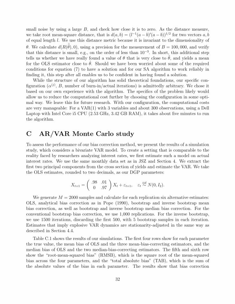
small noise by using a large B, and check how close it is to zero. As the distance measure,we take root mean-square distance, that is d(a, b) = (l−1(a− b)′(a− b))1/2 for two vectors a, bof equal length l. We use this distance metric because it is invariant to the dimensionality of

θ. We calculate d(R(ˆθ), 0), using a precision for the measurement of B = 100, 000, and verify

that this distance is small, e.g., on the order of less than 10−3. In short, this additional steptells us whether we have really found a value of θ that is very close to θ, and yields a meanfor the OLS estimator close to θ. Should we have been worried about some of the requiredconditions for equation (7) to have a solution and for our SA algorithm to work reliably infinding it, this step after all enables us to be confident in having found a solution.

While the structure of our algorithm has solid theoretical foundations, our specific con-figuration (α(j), B, number of burn-in/actual iterations) is admittedly arbitrary. We chose itbased on our own experience with the algorithm. The specifics of the problem likely wouldallow us to reduce the computational cost further by choosing the configuration in some opti-mal way. We leave this for future research. With our configuration, the computational costsare very manageable: For a VAR(1) with 3 variables and about 300 observations, using a DellLaptop with Intel Core i5 CPU (2.53 GHz, 3.42 GB RAM), it takes about five minutes to runthe algorithm.

C AR/VAR Monte Carlo study

To assess the performance of our bias correction method, we present the results of a simulationstudy, which considers a bivariate VAR model. To create a setting that is comparable to thereality faced by researchers analyzing interest rates, we first estimate such a model on actualinterest rates. We use the same monthly data set as in JSZ and Section 4. We extract thefirst two principal components from the cross section of yields and estimate the VAR. We takethe OLS estimates, rounded to two decimals, as our DGP parameters:

Xt+1 =

(

.98 .010 .97

)

Xt + εt+1, εtiid∼ N(0, I2).

We generate M = 2000 samples and calculate for each replication six alternative estimates:OLS, analytical bias correction as in Pope (1990), bootstrap and inverse bootstrap meanbias correction, as well as bootstrap and inverse bootstrap median bias correction. For theconventional bootstrap bias correction, we use 1,000 replications. For the inverse bootstrap,we use 1500 iterations, discarding the first 500, with 5 bootstrap samples in each iteration.Estimates that imply explosive VAR dynamics are stationarity-adjusted in the same way asdescribed in Section 4.4.

Table C.1 shows the results of our simulations. The first four rows show for each parameterthe true value, the mean bias of OLS and the three mean-bias-correcting estimators, and themedian bias of OLS and the two median-bias-correcting estimators. The fifth and sixth rowshow the “root-mean-squared bias” (RMSB), which is the square root of the mean-squaredbias across the four parameters, and the “total absolute bias” (TAB), which is the sum ofthe absolute values of the bias in each parameter. The results show that bias correction

32

Table C.1: VAR Monte Carlo simulation results

true Mean bias Median biasvalue OLS analytical bootstrap inv. boot. OLS bootstrap inv. boot.

Φ11 0.98 -0.0281 -0.0087 -0.0068 -0.0049 -0.0227 -0.0040 -0.0009Φ12 0.01 0.0015 -0.0007 -0.0004 -0.0007 0.0013 -0.0008 -0.0014Φ21 0.00 -0.0028 -0.0010 -0.0011 -0.0014 -0.0034 -0.0009 -0.0015Φ22 0.97 -0.0305 -0.0102 -0.0086 -0.0056 -0.0260 -0.0066 -0.0029RMSB 0.0208 0.0067 0.0055 0.0038 0.0174 0.0039 0.0018TAB 0.0629 0.0206 0.0168 0.0126 0.0534 0.0123 0.0066

max. eig. 0.98 -0.0154 0.0058 0.0081 0.0090 -0.0129 0.0091 0.0117half-life 34 -14.1930 13.7945 14.3122 23.0127 -18.0000 -10.0000 -7.0000IRF at h = 60 0.2976 -0.1726 0.0978 0.1433 0.1644 -0.2207 -0.0064 0.0503freq. expl. 0.25% 23.90% 35.00% 30.80% 0.25% 23.75% 21.50%

Notes: True values, mean bias, and median bias for parameters and persistence measures, andsummary statistics capturing total bias for the VAR Monte Carlo study. For details refer to thetext.

significantly reduces the small-sample parameter bias. This holds for all three bias correctionmethods, and for both mean and median bias. The total absolute bias is reduced by about 75%using the bootstrap. The inverse bootstrap is able to further reduce bias. It estimates mostelements of Φ with less bias, and reduces the measures of total bias. For the case of medianbias it roughly cuts the total parameter bias in half, compared to conventional bootstrap biascorrection.

The seventh to ninth rows show true values and the bias for three measures of persistence—the largest eigenvalue of Φ as well as the half-life and value of the IRF at a horizon of 60 periodsfor the response of the first variable to own shocks. To calculate the half-life we use the sameapproach as in Kilian and Zha (2002), with a cutoff of 500 periods—mean and median of thehalf-life are calculated across those replications for which it is available, which consequentlyexcludes values for which the half-life would be larger than 500.

The downward bias in estimated persistence for the OLS estimator is sizable. The half-life and long-horizon IRF are on average half as large as for the true DGP. Bias correctionincreases the estimated persistence significantly, and the dramatic downward bias in the largesteigenvalue disappears. Notably, for mean bias, the bias corrected estimates tend to be evenmore persistent than the DGP, whereas for median bias, they get the persistence about right.Conventional bootstrap and inverse bootstrap bias correction display similar performance interms of the implied persistence of the estimates.

The last row shows the frequency with which explosive eigenvalues occur. Evidently,although the DGP is stationary and the estimated model is correctly specified, there is asizable probability that the realized value of the OLS estimator is such that bias correctionleads to explosive estimates. Consequently, in practice one will often have to perform sometype of stationarity adjustment to ensure that estimated dynamics are not explosive. Themethod used in this paper, following Kilian (1998b), is admittedly ad hoc, and there is room

33

Table D.1: Maximally-flexible DTSM – summary statistics

OLS mean-BC median-BCanalytical bootstrap inv. boot. bootstrap inv.boot.

max(eig(Φ)) 0.9678 0.9961 0.9999 0.9991 0.9953 0.9946half-life 24 147 n.a. 265 128 132IRF at 5y 0.16 0.75 0.95 0.93 0.72 0.75

σ(f47,48t ) 1.392 1.392 1.392 1.392 1.392 1.392

σ(f47,48t ) 0.388 1.206 1.431 1.635 1.178 1.333

σ(ftp47,48t ) 1.301 1.216 1.322 1.656 1.254 1.430

Notes: Summary statistics for OLS and bias-corrected estimates of the DTSM in Joslin et al.(2011). First row: maximum eigenvalue of the estimated Φ. Second and third row: half-life andvalue of the impulse response function at the five-year horizon for the response of the level factor toa level shock. Rows six to eight show sample standard deviations of the fitted 47-to-48-monthforward rates and of the corresponding risk-neutral forward rates and forward term premia.

for future methodological improvement for reducing bias under the restriction of stationarity.We draw two conclusions from this simulation study: First, both the bootstrap and in-

verse bootstrap are useful and reliable methods to reduce the bias in OLS estimates of VARparameters. Second, the inverse bootstrap is a superior bias correction method compared toanalytical or bootstrap correction in a setting like ours, because it reduces higher-order biasand hence further improves the accuracy of the parameter estimates.

D Maximally-flexible DTSM: alternative bias correc-

tion methods

In the main text we present bias-corrected DTSM estimates that are obtained by applyinginverse bootstrap bias correction. Here we compare the results for the maximally-flexiblemodel of Section 4 to those obtained using alternative bias correction methods.

Table D.1 shows the summary statistics for six alternative sets of estimates: OLS, analyticalmean bias correction, bootstrap mean bias correction, inverse bootstrap mean bias correction,bootstrap median bias correction, and inverse bootstrap median bias correction. Correctingfor mean bias using the bootstrap leads to explosive VAR dynamics, so we apply Kilian’sstationarity adjustment in this case—for the resulting Φ matrix the IRF does not fall below0.5 within 40 years, our cutoff for half-life calculation as in Kilian and Zha (2002).

There are some differences in results across bias correction methods. Analytical bias cor-rection leads to a less persistent VAR system than inverse bootstrap bias correction. But thekey result is robust to using these alternative approaches: The persistence is substantiallyincreased by bias correction, so that short rate forecasts and risk-neutral rates are much morevolatile than for OLS. In practice, a researcher will likely use that method for bias correctionthat (s)he is most comfortable with on practical or theoretical grounds. For us, this is theinverse bootstrap method.

34

Table E.1: DTSM Monte Carlo study – parameter bias

Mean bias Median biasDGP OLS Mean-BC OLS Median-BC

1200µ -0.343 -0.219 0.077 -0.363 0.142 -0.013 -0.167 0.062 -0.011 -0.275 0.102 -0.012 -0.091 0.030 -0.010Φ 0.996 0.001 0.440 -0.024 0.025 -0.010 -0.010 0.012 0.010 -0.020 0.024 -0.001 -0.005 0.009 0.015

-0.001 0.990 0.352 0.006 -0.022 0.002 0.003 -0.009 -0.002 0.005 -0.018 0.002 0.001 -0.005 0.0010 0.001 0.873 -0.003 -0.003 -0.023 -0.001 -0.001 -0.004 -0.002 -0.002 -0.017 -0.001 -0.001 0.000

1200rQ∞ 8.647 -0.852 -0.822 -0.675 -0.683λQ 0.998 0.952 0.929 -0.001 0.000 -0.004 -0.001 -0.001 -0.004 -0.001 0.004 -0.007 -0.001 0.003 -0.007

1200Σ 0.643 0 0 -0.020 0 0 -0.015 0 0 -0.022 0 0 -0.016 0 0-0.146 0.210 0 0.005 0.013 0 0.004 0.014 0 0.006 0.012 0 0.005 0.014 00.063 -0.011 0.087 -0.002 0.004 0.027 -0.001 0.004 0.028 -0.002 0.004 0.027 -0.001 0.004 0.028

Notes: DGP parameter values, mean bias of OLS and Mean-BC estimates, and median bias of OLSand Median-BC estimates. For details refer to main text.

E Parameter bias in DTSM Monte Carlo study

In Table E.1 we show the DGP parameters that are used to simulate interest rate data fromthe DTSM, as well as mean and median parameter bias of the alternative estimates. Themean bias is shown for the OLS and Mean-BC estimates, whereas the median bias is shownfor the OLS and Median-BC estimates.

The bias in the estimates of VAR parameters µ and Φ is sizable for the OLS estimates.As expected, the bias-corrected estimates generally display reduced bias.

With regard to the Q-measure parameters, the values of λQ are estimated very accuratelyfor all three estimators. This confirms the intuition that in DTSM estimation, cross-sectionalinformation helps to pin down the parameters determining cross-sectional loadings very pre-cisely. The risk-neutral long-run mean rQ∞ is estimated with a slight downward bias by allestimators because the largest root under Q is very close to one, which naturally makes in-ference about the long-run mean under Q difficult. This has motivated some researchers torestrict the largest root under Q to one and rQ∞ to zero, in which case the long end of the yieldcurve is determined by a level factor (Bauer, 2011a; Christensen et al., 2011).

In sum, bias-corrected estimation methods reduce bias in estimates of the VAR parametersin comparison to MLE, whereas the remaining parameters are estimated with similar accuracy.

35

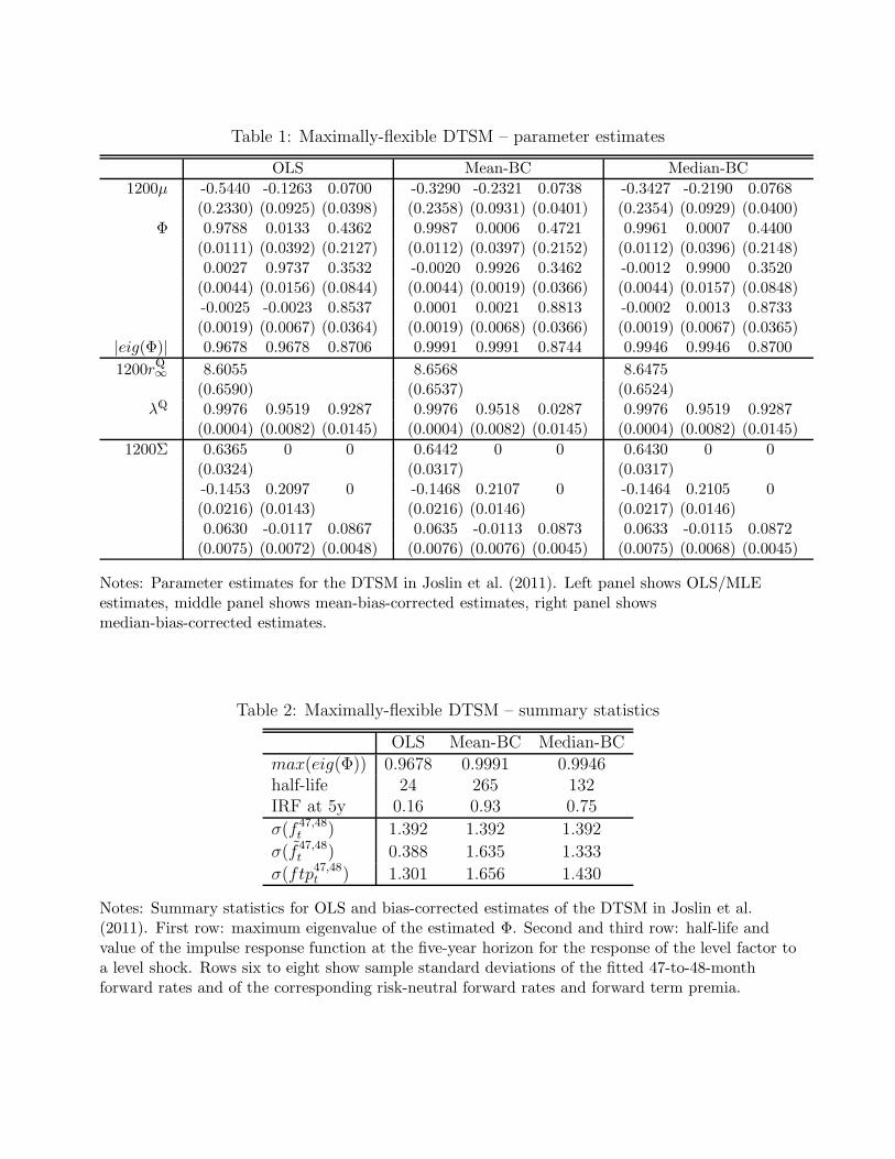
Table 1: Maximally-flexible DTSM – parameter estimates

OLS Mean-BC Median-BC

1200µ -0.5440 -0.1263 0.0700 -0.3290 -0.2321 0.0738 -0.3427 -0.2190 0.0768(0.2330) (0.0925) (0.0398) (0.2358) (0.0931) (0.0401) (0.2354) (0.0929) (0.0400)

Φ 0.9788 0.0133 0.4362 0.9987 0.0006 0.4721 0.9961 0.0007 0.4400(0.0111) (0.0392) (0.2127) (0.0112) (0.0397) (0.2152) (0.0112) (0.0396) (0.2148)0.0027 0.9737 0.3532 -0.0020 0.9926 0.3462 -0.0012 0.9900 0.3520(0.0044) (0.0156) (0.0844) (0.0044) (0.0019) (0.0366) (0.0044) (0.0157) (0.0848)-0.0025 -0.0023 0.8537 0.0001 0.0021 0.8813 -0.0002 0.0013 0.8733(0.0019) (0.0067) (0.0364) (0.0019) (0.0068) (0.0366) (0.0019) (0.0067) (0.0365)

|eig(Φ)| 0.9678 0.9678 0.8706 0.9991 0.9991 0.8744 0.9946 0.9946 0.8700

1200rQ∞ 8.6055 8.6568 8.6475(0.6590) (0.6537) (0.6524)

λQ 0.9976 0.9519 0.9287 0.9976 0.9518 0.0287 0.9976 0.9519 0.9287(0.0004) (0.0082) (0.0145) (0.0004) (0.0082) (0.0145) (0.0004) (0.0082) (0.0145)

1200Σ 0.6365 0 0 0.6442 0 0 0.6430 0 0(0.0324) (0.0317) (0.0317)-0.1453 0.2097 0 -0.1468 0.2107 0 -0.1464 0.2105 0(0.0216) (0.0143) (0.0216) (0.0146) (0.0217) (0.0146)0.0630 -0.0117 0.0867 0.0635 -0.0113 0.0873 0.0633 -0.0115 0.0872(0.0075) (0.0072) (0.0048) (0.0076) (0.0076) (0.0045) (0.0075) (0.0068) (0.0045)

Notes: Parameter estimates for the DTSM in Joslin et al. (2011). Left panel shows OLS/MLEestimates, middle panel shows mean-bias-corrected estimates, right panel showsmedian-bias-corrected estimates.

Table 2: Maximally-flexible DTSM – summary statistics

OLS Mean-BC Median-BCmax(eig(Φ)) 0.9678 0.9991 0.9946half-life 24 265 132IRF at 5y 0.16 0.93 0.75

σ(f 47,48t ) 1.392 1.392 1.392

σ(f 47,48t ) 0.388 1.635 1.333

σ(ftp47,48t ) 1.301 1.656 1.430

Notes: Summary statistics for OLS and bias-corrected estimates of the DTSM in Joslin et al.(2011). First row: maximum eigenvalue of the estimated Φ. Second and third row: half-life andvalue of the impulse response function at the five-year horizon for the response of the level factor toa level shock. Rows six to eight show sample standard deviations of the fitted 47-to-48-monthforward rates and of the corresponding risk-neutral forward rates and forward term premia.

Table 3: DTSM Monte Carlo study – summary statistics

Mean MedianDGP OLS Mean-BC Median-BC DGP OLS Mean-BC Median-BC

max(eig(Φ)) 0.9946 0.9805 0.9965 0.9956 0.9946 0.9831 0.9993 0.9993half-life 133 40.54 105.65 98.89 133 22.00 40.00 38.00IRF at 5y 0.75 0.20 0.52 0.51 0.75 0.14 0.55 0.52

σ(f47,48t ) 1.57 1.58 1.58 1.58 1.45 1.45 1.45 1.46

σ(f47,48t ) 1.74 1.17 1.95 1.89 1.63 0.97 1.81 1.77

σ(ftp47,48t ) 1.84 1.73 2.09 2.04 1.72 1.49 1.91 1.87

RMSE(f47,48t ) 0.01 0.01 0.01 0.01 0.01 0.01

RMSE(f47,48t ) 1.37 1.20 1.18 1.31 1.13 1.11

RMSE(ftp47,48t ) 1.37 1.20 1.18 1.31 1.13 1.11

Notes: Summary statistics for persistence, variability, and accuracy of estimated rates and premiain DTSM Monte Carlo study. First three rows show true values (DGP) and means/medians ofestimated values for the largest root of Φ, the half-life in months (across estimates that have ahalf-life of less than 40 years), and the value of the impulse response function (IRF) at the five-yearhorizon for response of the first risk factor to own shocks. Rows four to six show means/medians ofsample standard deviations of forward rates, risk-neutral forward rates, and forward premia. Lastthree rows show means/medians of root-mean-squared errors (RMSE) for estimated rates andpremia.Volatilities and RMSE’s are in annualized percentage points. For details refer to main text.

Table 4: Restricted DTSM – parameter estimates

OLS-UR OLS-R BC-R

1200Σλ0 0.3146 0.1159 0.0790 0.3329 0.1015 0.0652 0.3274 0.1006 0.0537(0.2293) (0.0708) (0.0260) (0.1240) (0.0512) (0.0186) (0.1250) (0.0513) (0.0187)

Σλ1 -0.0116 -0.1303 -0.0340 -0.0161 -0.1229 0 -0.0092 -0.1271 0(0.0074) (0.0439) (0.2773) (0.0060) (0.0358) (0.0060) (0.0361)0.0012 -0.0113 -0.1577 0 0 -0.1552 0 0 -0.1420(0.0023) (0.0136) (0.0856) (0.0789) (0.0792)-0.0008 -0.0021 -0.1043 0 0 -0.1065 0 0 -0.0886(0.0008) (0.0050) (0.0315) (0.0287) (0.0288)

1200rQ 15.0635 15.0609 15.1111(0.5418) (0.5420) (0.5456)

λQ 0.9976 0.9488 0.9563 0.9976 0.9490 0.9561 0.9976 0.9491 0.9561(0.0001) (0.0072) (0.0058) (0.0001) (0.0076) (0.0062) (0.0001) (0.0077) (0.0063)

1200Σ 0.7264 0 0 0.7261 0 0 0.7327 0 0(0.0284) (0.0284) (0.0287)0.0982 0.2125 0 0.0981 0.2125 0 0.0990 0.2132 0(0.0117) (0.0078) (0.0117) (0.0078) (0.0117) (0.0079)-0.0291 0.0211 0.0728 -0.0291 0.0211 0.0728 -0.0292 0.0212 0.0729(0.0044) (0.0040) (0.0029) (0.0044) (0.0040) (0.0029) (0.0044) (0.0040) (0.0029)

Notes: Conventional parameter estimates for maximally-flexible model specification (OLS-UR), aswell as conventional (OLS-R) and bias-corrected (BC-R) estimates of the model with zerorestrictions on risk price parameters.

Table 5: Restricted DTSM – summary statistics

OLS-UR OLS-R BC-Rmax(eig(Φ)) 0.9909 0.9904 0.9953half-life 64 44 92IRF at 5y 0.52 0.41 0.60

σ(f 61,120t ) 1.755 1.755 1.755

σ(f 61,120t ) 1.148 1.058 1.705

σ(ftp61,120t ) 1.230 1.369 1.425

Notes: Summary statistics for OLS estimates of unrestricted model (OLS-UR), as well as OLS andbias corrected estimates of restricted model. Persistence measures and standard deviations of thefitted five-to-ten-year forward rates and of the corresponding risk-neutral forward rates and forwardterm premia.

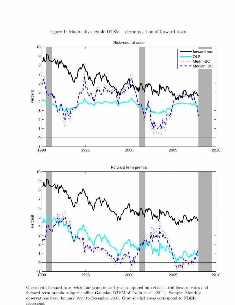
Figure 1: Maximally-flexible DTSM – decomposition of forward ratesP

erce

nt

Risk−neutral rates

1990 1995 2000 2005 2010−1

0

1

2

3

4

5

6

7

8

9

10forward rateOLSMean−BCMedian−BC

Per

cent

Forward term premia

1990 1995 2000 2005 2010−1

0

1

2

3

4

5

6

7

8

9

10

One-month forward rates with four years maturity, decomposed into risk-neutral forward rates andforward term premia using the affine Gaussian DTSM of Joslin et al. (2011). Sample: Monthlyobservations from January 1990 to December 2007. Gray shaded areas correspond to NBERrecessions.

Figure 2: Risk price restrictions – decomposition of forward ratesP

erce

nt

Risk−neutral rates

1985 1990 1995 2000 2005 2010

0

2

4

6

8

10

12

Per

cent

Forward term premia

1985 1990 1995 2000 2005 2010

0

2

4

6

8

10

12

forward rateOLS−UROLS−RBC−R

Decomposition of five-to-ten year forward rates into risk-neutral and term premium componentsusing alternative DTSM estimates Sample: Monthly observations from January 1985 to December2011. Gray shaded areas correspond to NBER recessions.