1

CORPORATION TAX INCIDENCE:

REFLECTIONS ON WHAT IS KNOWN,

UNKNOWN AND UNKNOWABLE

Arnold C. Harberger

University of California, Los Angeles

Paper prepared for a Conference

“Is It Time For Fundamental Tax Reform:

The Known, Unknown, and Unknowable?”

James A. Baker III

Institute for Public Policy

Rice University

April 2006

2

About The Unknowable

Asked to comment on a topic as celestial as “the unknowable”, I am inclined to deal with

the most basic things first. And obviously, the strictures imposed by a general-equilibrium

framework have to be counted among the most basic elements in the analysis of tax incidence --

not just that of the corporation income tax, but of any tax whatsoever.

The problem, of course, lies in the fact that we cannot handle the incidence of a tax in a

general-equilibrium setting without knowing (or making assumptions about) how the receipts of

that tax are going to be spent, and what other distortions are deemed to be present in the

economy. Since there are millions of different ways in which the receipts of our tax might be

spent, the millions of combinations of other distortions that might be present when the taxes

imposed, increased, decreased or removed, it looks as if one can get “millions squared” different

answers to the simple question “What is the incidence of a single specific tax (or tax provision)”.

Economists have had to face this problem from the outset, but have not articulated it

often enough or well enough for it to be clearly and widely recognized. To my mind, we cannot

speak of the incidence of the corporation income tax in a way that somehow covers all of the

“millions squared” possibilities of how the money will be spent, and in the presence of what

specific set of other distortions.

What we want is some way of saying, this is the essential answer to the incidence

question. And I believe we have found such a way. For incidence analysis this solution consists

of assuming that the government spends its tax receipts in a fashion similar to the way that the

people themselves would have spent the money. This assumption enables us to use a single set

of demand functions, thus making the analysis even simpler than it would be with any other way

3

of handling government demand. For our convenience, let us call this the “demand neutrality”

assumption.

The demand neutrality assumption allows us, at least in principle, to divide a real-world

problem into modules. If we think of an increase in the corporation income tax, with the

proceeds being spent on a new airport, we have an incidence module in which the government

raises the money and spends it according to the “people’s” demand function, and an expenditure-

shifting module in which the government introduces its own airport-project demand function in

place of the scaled-down version of the people’s demand function that describes government

demand under the assumption of demand neutrality. This possibility, of breaking the general-

equilibrium problem into an incidence module and an expenditure-shift module, is incredibly

helpful. For, in particular with regard to our present focus, it enables us to conceive of such a

thing as an essential answer to the incidence question.1

I would like readers to bear in mind that this essential answer to the incidence question is

built on quite subtle foundations. I sometimes say that this answer lives in economists’ minds,

more than in the real world. Well applied, it certainly has relevance for the real world, but

certainly the real world will never replicate the mental experiments we make when we engage in

our “professional” incidence analysis.

1Economists have to make a similar assumption when dealing with the measurement of

the efficiency costs (excess burdens) of taxation. Here the practice has been to use the convention of “lump-sum taxes and transfers” to keep individuals and households on their original set of demand functions. In this case, module1would deal with the efficiency costs of the corporation income tax, with lump sum taxes and transfers keeping the purchasing power of individuals and households the same as before, and module 2 would deal with the efficiency effects of taking away these lump sum taxes and transfers and using the net proceeds to finance the airport project.

4

* * * *

Economists are quite familiar with the havoc that pre-existing distortions can wreak when

we are analyzing the efficiency costs of taxation. The triangle of efficiency cost (-1/2 T6∆X6)

generated by imposing a new tax T6 on good X6 can be dwarfed by the induced efficiency cost

or gain

∆∂∂

≠Σ 6T]6T/jX[jT5

1j that comes from the reactions in the markets for X1 through

X5, all of them here assumed to have pre-existing taxes or subsidies. Standard general-

equilibrium efficiency analysis tells us that T6 always generates net efficiency costs in the

absence of other distortions, but that in their presence it can bring either net benefits (e.g., a

pollution tax or a tariff on a key input into the domestic production of an already-protected final

product) or enhanced net costs (e.g., a tax on wheat when corn, a substitute in both demand and

supply, is already subsidized).

Something similar happens when the focus of our analysis is on incidence. In this case,

the induced responses of commodities with existing taxes or subsidies simply generate an

additional (or reduced) amount of tax, [∑Tj(∂Xj/∂T6)∆T6] the incidence of which we have to

analyze. Thus, for example, when a new or increased corporation income tax causes capital to

move from the corporate sector to the housing sector, it is in principle fully appropriate to

include in an incidence analysis the additional property taxes and housing subsidies and other tax

offsets that this move generates.

But this is not what we typically talk about on the subject of corporation tax incidence.

Why? My answer is that the pattern of other taxes and subsidies is too time-and-place-specific

for us to be able to carry on a reasonable discussion focused on the corporation income tax. To

5

me, it is just like the question of how the government is going to spend the money that a tax

generates. Just as there are a million ways that money can be spent, so also there are a million

patterns of other taxes and their rates, into which we could “insert” a corporation income tax of a

particular configuration (e.g., striking all capital income, or just the returns to equity, integrated

on dividends, on grossed-up-dividends on post-tax corporate profits, or pre-tax corporate profits,

or not integrated at all with the personal income tax).

Readers should not infer that I am throwing in the towel with these remarks -- that I am

giving up in the face of a task that seems utterly hopeless. No -- instead of this, I am trying to

emphasize that we simply must work with constructs that are artificial -- in the sense of not

being found in the real world -- but useful in enabling us to think through problems that

otherwise would be totally daunting.

On the whole, what the profession has done, is go down one of two roads. The first “pure

incidence theory”, entails making the demand neutrality assumption, plus that of “no other

distortions”. These assumptions give us a pretty pure module to work with, and also a pretty

clear field on which to wage our intellectual battles. This is the road that most of our incidence

literature has taken, and on which I will try to stay in the present paper.

The second road is that of computable general equilibrium (CGE) analysis. Here it is

possible to simulate the main skeleton of a real-world tax-expenditure system, and to see how the

relative real incomes (or utilities) of different subgroups of the population would change if that

system were altered in specific ways. For this road to be fruitful, the modeling and also the

calibration to the actual tax-expenditure system of the country, must be of a very high

professional quality. My impression is that most exercises of this type end up delving into the

incidence of the entire tax (or tax-expenditure) system, and not into the incidence of particular

6

elements of that system (such as the corporation income tax, taken by itself). Not being myself a

traveler on this second road, I will let these few remarks suffice.

* * * *

As things stand, our main line of attack on the problem has been to build models with

resource constraints, production and demand functions, etc., and to compare the results of

running these models with no taxes at all on the one hand, and with a corporation income tax on

the other. Personally I like this approach, which I think, if well executed, captures the essentials

of economic behavior and economic structure, while allowing us to keep the analysis simple

enough for us to understand how the machinery works. Making models more realistic by adding

complications quickly gets us into situations where we either accept the model’s answers on

blind faith, or else remain skeptical about the results because we cannot internalize the

mechanism that produced them. To be useful, then, our bare-bones skeleton has to be a very

good one -- capturing essential elements and leaving aside frills. And it is perfectly reasonable

that there should be discussion and debate among professionals as to how one can best represent

an economy’s most essential elements.

In all of this I am ready to classify as known the fact that economic behavior is well

represented by things like demand and production functions, market equilibrium, adding up, etc.

-- i.e., the bare bones of simple general-equilibrium modeling. Similarly, I would classify as

knowable the key parameters of demand and production functions. These are knowable not

down to decimals, but certainly as general orders of magnitude. I can “know” that the elasticity

of substitution between tradables and nontradables as composite commodities is well below

unity, but that does not deny that many specific tradables will have quite good substitutes among

the thousands of elements in the great basket that we call nontradables. Thus, if what I need for

7

my modeling is the broad relation between tradables and nontradables (a relation that is

modulated by the real exchange rate), and if what I’m looking for is a rough order of magnitude,

then I believe the relevant elasticity is “knowable”. But if what I need is great precision about

this aggregate elasticity, or if I need to know a lot of component demand relationships between

specific tradables and specific nontradables, then I would, rather sadly, have to say that we are

dipping our toes into the domain of the unknowable.

Where we really get into that domain, however, is when we consider the settings in which

our scenarios will play. If the corporation income tax is raised or lowered, what will be the

money be spent on, or which expenditures will be cut, or which other taxes lowered or raised?

And as we debate this issue in our seminars, how can we know the set of surrounding taxes and

subsidies that will exist if and when our country (or some other country) decides to make a major

shift in its rate of corporation tax? These are areas that I, for one, would want quite seriously to

classify as unknowable.

Open or Closed Economy -- A Matter of Scenarios

Too much paper and ink has been wasted on discussions that act as if, to be relevant, one

must choose between an open and a closed economy model to represent the real world. This is

not the right way to focus on the problem. Instead, it is much more meaningful to think of

scenarios, or classes of disturbances that we want to analyze. In a nutshell, if one country (or a

smallish subset of countries) decides to raise or lower its rate of corporation income tax, the

appropriate model is one of an open economy. On the other hand, if all countries (or a set of big

countries making up most of the world economy) choose to move their CIT rates in more-or-less

parallel fashion, then the appropriate model is one of a closed economy.

8

I think that the big, world-level story of the past few decades, in which we have seen a

pretty general worldwide reduction in corporate tax rates, is one for which the closed economy

model makes more sense than the open-economy one. But that is not the main point that I would

like to make. The main point is that both models are relevant, with the closed economy model

dealing with a scenario in which all countries impose (or raise or lower) a similar rate of

corporation income tax together, and with the open economy model dealing with the case in

which one country (or a small group of countries) does so alone, with the rest of the world

standing pat. In this light, it makes no sense to ask economists to choose between the models.

Which one to use depends on a pretty straightforward way on the type of problem we economists

are trying to analyze.

Treating the Corporation Income Tax As a “Partial Factor Tax”

One tradition that I would like to stick to in the present paper is that of treating the

corporation income tax as a tax on the income from capital in a subsection of the economy

known as the corporate sector. In a closed economy it would be a tax Tkx on the income from

capital in X, the corporate sector, and not on that in Y, the noncorporate sector. In an open

economy model, it would be a tax on the income from capital in A (the tradable-goods

corporate sector, e.g., manufacturing) and in B (the nontradable-goods corporate sector, e.g.,

public utilities and transport). This tax would not affect the income from capital in C (the

noncorporate tradable sector, e.g., agriculture) or in D (the noncorporate, nontradable sector,

e.g., services). This classification comes pretty close to reality, if one thinks of the effective rate

of CIT in a sector being that sector’s corporate tax collections divided by that sector’s total

income from capital. By this measure the “corporate” sectoral rates Tka and Tkb are typically

9

much higher than the “noncorporate” sectoral rates Tkc and Tkd, sufficiently so that we can

safely neglect the latter.2

Even with this simplification, there is no reason why, in the real world Tka and Tkb

should be the same, but for the purpose of getting a straightforward answer to the incidence

question, we will consider them so.3

My Own 4-Sector Story

This story goes back to around 1970, to my public finance classes at the University of

Chicago. I had been teaching the closed-economy model of incidence for more than a decade,

and had just completed that exercise in this particular class. But this class was different from its

predecessors, in that its members had been exposed to the flowering of the monetary approach to

the balance of payments (under Harry Johnson and Robert Mundell) and its related small-open-

economy models of international trade. Hence it was quite natural for a couple of these students

to rise in class with the question -- “How does this all work in the open economy.”

2More elegantly, we could consider that the average rate of CIT collections in C and D )cdT( as a general tax on the income of all capital, the incidence of which would fall

exclusively on the income from capital, assuming that factor to be in fixed supply (Ka + Kb + Kc + Kd = ).K Then the partial factor taxes would be ),cdTaT( − ),cdTbT( − ),cdTcT( − and

).cdTdT( − We would then neglect )cdTTc( − and )cdTdT( − as being small, and indeed, averaging out to zero over the two nontradable sectors (C and D).

3The main reason why Tka and Tkb would differ in the real world would not be

different official rates of tax on corporate profits, but rather different ratios of debt to equity, as between “manufacturing” on the one hand and “public utilities plus transport” on the other. Typically, the latter sector has significantly higher equilibrium debt-equity ratios, thus causing its “effective” rate of corporation income tax to be lower.

10

Being then perhaps faster on my feet than I am now, I quickly responded, “Let’s find

out”, and moved directly to the equations of the closed-economy model.

Since the model had only two sectors, X (corporate) and Y (noncorporate), I really had

only two options: make X tradable and Y nontradable, or vice versa. So then and there, in

that classroom, we worked out the answers.

If Y is the tradable sector, its price-formation equation:

(1) dpy = gkdpk + gLdpL

would be the relevant one (gk and gL are the shares of capital and labor in the production costs

of Y). Standard open-economy assumptions would say that the small open economy would be a

price-taker for tradables, and a price-taker in the world capital market. We would therefore

impose dpy = dpk = 0, which would lead us to the conclusion that dpL = 0. This, in turn, would

mean that the price of the nontradable, corporate product (X) would rise to reflect the full

amount of the tax.

(2) dpx = fk(dpk+Tkx) + fLdpL.

(Here fk and fL are the shares of the two factors in the production of X.) With dpk and dpL

equal to zero, this yields dpx = fkTka. That is, “consumers” of the taxed sector’s output would

bear the tax. To allocate the tax to labor and capital, we would do so by saying that they would

share the tax in accordance with their respective demands for X, labor bearing βLxKxTkx and

capital bearing βkxKxTkx, the β’s being the fractions in which product X ended up being

bought by workers on the one hand and owners of capital on the other (with, of course, βLx +

βkx = 1).

11

This result was interesting, in that it was identical to that in the closed economy case,

where Sy, the elasticity of substitution between labor and capital in the Y industry, was

infinite. That case also led to no change in the relative prices of labor and capital in the Y

industry, and (with pL as the numeraire in that closed-economy case) to no change in py , and

to dpx = fkTkx.

This surprised us a bit, but we did not dawdle over this result. Instead we went on to the

case where X rather than Y was the tradable good. Inserting dpx = dpk = 0 into equation (2)

we got

(3) 0 = fkTkx + fLdpL.

With all initial prices set equal to 1 (an innocuous assumption involving only the choice of units

in which we measure products and factors), we have fk = Kx/X and fL = Lx/X. Hence (3)

resolves into

(3’) LxdpL = -KxTkx.

This is a super-intuitive answer. For what it says is that if px cannot go up, and pk cannot go

down (owing to the international mobility of X and K), then the only way activity X can stay

in business is for pL to go down by enough to absorb (in industry X itself) the full weight of

the tax paid by that industry.

But if pL goes down in industry X it must also go down in industry Y. So labor as a

whole loses KxTkx[(Lx+Ly)/Lx]. That is, labor bears, in the first instance (Lx+Ly)/Lx times

the burden of the tax.

Part of this burden will come back to laborers, of course, in their role as consumers of the

now nontradable good, Y. Its price will go down to reflect the loss sustained by workers in the

12

Y industry, and this price reduction will redound as a benefit to labor and capital in their role as

consumers. Hence labor will end up bearing [Lx+Ly(1-βLy)]dpL, capital will gain -

βkyLydpL, and the government will get tax revenue equal to -LxdpL. (Recall that dpL is

negative; see equation (3’)).

This result, then, said that not only would labor bear the burden of the tax in this open-

economy scenario; it would bear significantly more than the full burden. When this result came

out in class, we almost fell off our chairs. For in the closed-economy case we had studied an

outcome in which capital would bear [Kx+Ky(1-βky)]Tkx, labor would gain βLyKyTkx, and

the government would get KxTkx. This result emerged when Sx, the elasticity of substitution

between labor and capital in the corporate sector, was infinite. Now, looking at the open-

economy case, we got the mirror image of this result, but with labor rather than capital being the

unlucky factor that ends up bearing more than the full burden of the tax.

So we ended up surprised, perhaps bemused, by the open economy results, particularly

the uncanny parallelism between what we now obtained in the open-economy case, and what we

had previously gotten in the closed economy case -- uncanny because what had earlier been the

fate of owners of capital was now being visited upon the labor factor.

I was at least sufficiently attracted by this result that I kept showing it to my classes in

the years following 1970. But I never really liked it, in the sense of feeling it was yielding

important insights into how the corporation income tax might really work. This suit of clothes

just did not seem to fit right on the customer.

I have no good excuse, other than always being busy, always struggling to fulfill duties

and commitments, for why I did not right away seek a suit of clothes that fit better. But I did

not. It was not until around 1980, when I was involved in guiding the Ph.D. dissertation work of

13

Arturo Fernandez Perez, that all of a sudden I experienced my personal “epiphany” on this

subject. That came with the realization that what the problem called for was the four-sector

model of manufacturing (A), public utilities and transport (B), agriculture (C) and services

(D). This led to a straightforward, highly intuitive and easily communicated story of corporation

tax incidence in the open economy.

The key sector in this story is the corporate tradable sector (manufacturing). For this

sector, now A, the old story of X as the tradable sector still applies. The price of the product

pa cannot change, the return to capital pk cannot change, so when the tax wedge Tka is

inserted in the price formation equation for A, we get KaTka = -LadpL. This determines the

whole pattern of incidence and price formation throughout the economy.

In manufacturing, wages have to go down as shown; otherwise we must go to a corner

solution with zero output. And they must go down so as precisely to offset the added cost

imposed by the tax wedge. Thus dpL for the whole economy is determined in the

manufacturing (corporate tradable) sector. The reduced wage causes pd, the price level of

services, to go down. The price level for agriculture cannot go down because it is determined

internationally (for the small open economy). Here we introduced an important “trick”, by

allowing land to be a significant productive factor in agriculture, and by keeping reproducible

capital (K) out of agriculture. With this simplification, the lower wage results in increasing

land rents, but of course with no change in the international price level of agriculture products.

This leaves public utilities and transport, sector B, which we assume to be subject to the same

partial tax on capital (Tka) as sector A. Hence if the shares of capital and labor are the same in

B as in A, the price of B will not change. It is more likely, however, that B will be

significantly more capital intensive than A, in which case pb will have to rise to reflect that

14

portion of the (now greater) tax wedge in B that is not absorbed by the decline in pL. Since

product B is nontradable, there is no impediment to this rise in its price.

Once I had internalized this vision, I became willing to talk in public about open-

economy tax incidence, and I felt no reluctance to peddle the notion, not just of labor tending to

fully bear, but more than that -- to more than fully bear the burden of the corporation income tax.

This would be even more certain in a small open economy than in a very big one, because in the

big economy case some of the impact of the tax might be absorbed through a general worldwide

fall in the rate of return to capital. And I pretty much hold to this judgment to this day, even

after having experimented with various margins.

The Small Open Economy -- A Price-Taker In the World Capital Market

Obviously, one way in which one could get different results from those outlined above

would be if the (net-of-tax) rate of return to capital would itself move as a consequence of a

country’s having (versus not having) a corporation income tax. We first try to deal with this case

for the small open economy. The first step is to recognize that we have no reason to postulate

that the world rate of return will be significantly different, with the small country having or not

having a CIT. The tougher question is whether in the small country itself it is plausible that the

rate of return would be different with the tax than without it. Here again I say no, but I recognize

that the argument is much more subtle than the above. As a decades-long student of real

exchange rate behavior in developing countries, I definitely reject the idea that such a country

faces a completely flat supply curve of foreign funds to its market. The supply curve of funds

has to be upward sloping, with respect to the real rate of return required. This may be thought of

as being based on increasing degrees of perceived country risk, or on other forces. But the main

point is that it depends on factors other than the presence or absence of a corporation income tax.

15

To make my point very clear, I want to model the small country as having no net borrowing from

abroad in the absence of the CIT and no net borrowing in its presence. The movement of funds

that takes place as a consequence of the imposition of a CIT in that country should, I think, be

viewed as a movement of the country’s residents’ own funds out of the country (as the

Argentines are said to have had, at times, as much as a year’s GDP worth of money stashed away

in Miami, New York, London, Paris, and other centers).

It is very important to realize that our standard comparative static modeling of the

incidence of the CIT does not examine the transition during which a significant chunk of the pre-

existing capital stock (in the no CIT case) moves abroad as a consequence of the imposition of

the CIT. Rather than look at this transition, the analysis looks at two steady-state equilibria --

one without the CIT and with a larger capital stock invested in the country, the other with the

CIT and with a smaller capital stock invested in the country. What I’m saying is that the

clearest, most natural assumption to make about these two steady-state equilibria is that in each

of them trade is balanced.4

4The alternative assumption is to treat the national income of the country as incorporating the return to the capital that its residents (the Argentines) shifted abroad as a consequence of the tax. Under this assumption one would assume not balanced trade but balanced payments with one piece of capital income shifting, from domestic source to foreign sources as a consequence of the tax. The natural result of this would be an appreciation of the equilibrium (steady-state) real exchange rate as a consequence of the tax, making tradables (both corporate and noncorporate) relatively cheaper, and nontradables (both corporate and noncorporate) relatively more expensive. I do not believe that this would make for an important modification of the incidence conclusions that we get, based on balanced trade in both the pre-tax and the post-tax equilibria. In any case, I see no basis for thinking that the equilibrium real rate of return on capital will be different, with or without the corporation income tax. The conclusion is that we should continue to treat the small open economy as a price-taker in the international capital market.

16

Capital Reallocations in the Large-Country Case

I have always thought of the United States as exemplifying the large-country case in

almost any context. In the particular case we are treating here this means that we should allow

for a possible fall in the worldwide real return to capital, as a consequence of the imposition of a

CIT in the U.S. Just as the rate of return will likely be driven down under a CIT in the closed

economy case, with capital shifting from the corporate to the noncorporate sector, so in the open

economy case capital will also run away from the corporate sectors (A and B). But now it has

two places to go -- to the local noncorporate sectors (C and D), and to the capital markets of

the rest of the world. One would naturally expect a smaller drop in the rate of return in the open

economy case than in the closed economy case, simply because of the existence of an additional

very large sponge (the rest of the world’s capital market) to help absorb the capital that is being

ejected from, in this case, the U.S. corporate sector, as a consequence of the tax.

But again I would reject any notion that a U.S. corporation income tax would by itself

cause a differential change in rates of after-tax return, here and abroad. For the big countries

there is really just one world capital market. Billions of dollars daily cross both the Atlantic and

the Pacific, seeking to gain as little as an eighth of a point of interest in covered interest

arbitrage. If ever there was a market in which the law of one price could be said to be regularly

and vigorously pursued by lots of economically potent and highly knowledgeable participants

(the great international banks and financial houses), this is it. So yes, we can have pk changing

in this large-country, open-economy scenario, but not differentially.

Pursuing an approach like this a decade ago, I developed a simple example5 which was

“rigged” so that owners of capital, all over the world, would bear a direct burden (unadjusted for

17

their role as consumers) that was precisely equal to what the U.S. government (the model one,

not the real one) got from a hypothetical corporation income tax levied only by the U.S. In that

numerical exercise the net-of-tax rate of return to capital (worldwide) dropped from 9 to 8

percent. Thus, a 1 percentage point fall in the return to capital, all over the world, was assumed

to create a loss to the owners of that capital, just equal to total U.S. CIT collections.

To complete this picture, we should note other gainers and losers. If capital as a whole

bears the full burden, and U.S. corporate capital bears only, say, 1/4 of it, the rest will be borne

by capital abroad. This will be matched by a gain to labor abroad, and a loss to foreign

landowners, who now will have to pay higher wages. In the U.S., landowners will gain from

lower wages, as will the consumers of services. Consumers will lose, however, as a consequence

of higher prices in the (capital-intensive) public utilities and transport sector. Consumers of

housing (worldwide) should gain as a result of the drop in the worldwide rate of return to capital.

But the assumed U.S. tax rate on the earnings of corporate capital was 50%. This meant

that in manufacturing, the “critical sector” (where the main action takes place), the gross-of-tax

return would rise to 16%. Only 1/8 of the tax “wedge” of 8% was absorbed by owners of capital

in that sector. The rest, with given prices of manufactured products, had to be borne by U.S.

labor. The wage of labor had to fall to the extent that U.S. labor in manufacturing suffered a loss

equal to 7/8 of U.S. CIT receipts from the manufacturing sector. But if only 20% of U.S. labor

was engaged in manufacturing, then the loss suffered by all U.S. labor would be 5 times as great,

equal to 35/8 of U.S. CIT receipts in manufacturing.

5See Arnold C. Harberger, “The ABCs of Corporation Tax Incidence: Insights Into the Open-Economy Case,” in American Council for Capital Formation, Tax Policy and Economic Growth (Washington, DC: ACCF, 1995), pp. 51-73.

18

In the present paper I will develop a similar scenario, adding extra details along the way.

The first such detail is the assumption that the U.S. stock of reproducible productive capital is

divided 1/4, 1/4, and 1/2 as between manufacturing, public utilities and transport, and services

(including those from housing). This means that half of CIT receipts come from the

manufacturing sector, so labor ends up bearing a burden equal to 35/16 of total U.S. CIT

receipts.

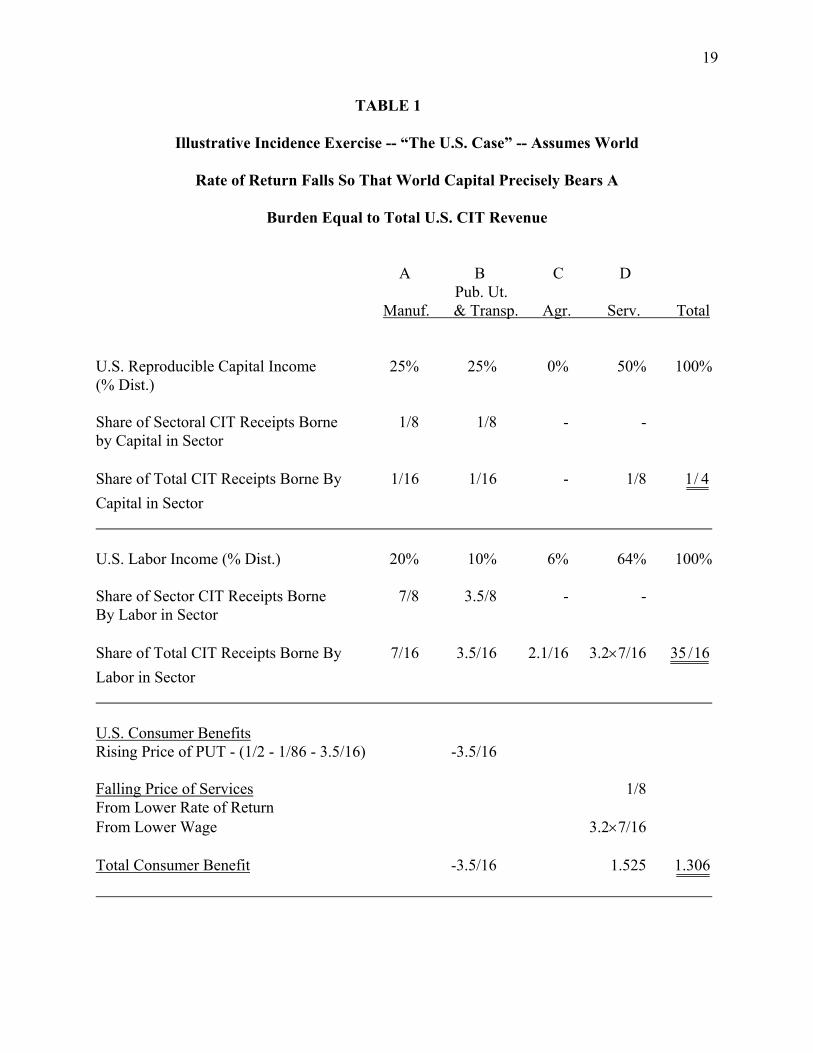
This and subsequent steps in the present exercise are illustrated in Table 1. The first

panel of this table focuses on the burdens borne by U.S. capital. As already noted, capital in

manufacturing bears 1/8 of the CIT receipts from manufacturing, which means 1/16 of total CIT

receipts. The public utilities and transport sector has a capital stock equal to that of

manufacturing, so its capital owners bear a cost of equal size. Since the services sector has twice

the capital of manufacturing, its capital owners bear twice the burden of those in sector A.

Taken together, the owners of U.S. capital bear, as factor owners, a burden equal to 1/4 of total

U.S. CIT receipts. The obvious inference is that foreign owners of capital bear a burden three

times this large. This would have its reflection in a roughly equal gain to foreign workers.

The underlined figure at the lower right corner of panel 1 gives the key summary statistic

of U.S. capital’s share of the burden.

Next we turn to U.S. labor. The second panel shows first, the assumed percentage

distribution of U.S. labor income. Second, we record the fact, already discussed, that labor in

manufacturing has to absorb 7/8 of the CIT tax wedge in manufacturing. Since sector B has only

half the labor force of sector A, but an equal capital stock, its labor bears a burden that is only

half as big, relative to general CIT revenues. Line 3 of panel 2 expresses labor’s losses as a

19

TABLE 1

Illustrative Incidence Exercise -- “The U.S. Case” -- Assumes World

Rate of Return Falls So That World Capital Precisely Bears A

Burden Equal to Total U.S. CIT Revenue

A B C D Pub. Ut. Manuf. & Transp. Agr. Serv. Total

U.S. Reproducible Capital Income 25% 25% 0% 50% 100% (% Dist.) Share of Sectoral CIT Receipts Borne 1/8 1/8 - - by Capital in Sector Share of Total CIT Receipts Borne By 1/16 1/16 - 1/8 4/1 Capital in Sector U.S. Labor Income (% Dist.) 20% 10% 6% 64% 100% Share of Sector CIT Receipts Borne 7/8 3.5/8 - - By Labor in Sector Share of Total CIT Receipts Borne By 7/16 3.5/16 2.1/16 3.2×7/16 16/35 Labor in Sector U.S. Consumer Benefits Rising Price of PUT - (1/2 - 1/86 - 3.5/16) -3.5/16 Falling Price of Services 1/8 From Lower Rate of Return From Lower Wage 3.2×7/16 Total Consumer Benefit -3.5/16 1.525 306.1

20

Table 1 (continued) A B C D Pub. Ut. Manuf. & Transp. Agr. Serv. Total

Allocation of U.S. Consumer Benefit (as Fraction of Total U.S. CIT Revenue) Allocated to Capital (.30 × 1.306) .392 Allocated to Labor (.68 × 1.306) .888 Allocated to Landowners (02 × 1.306) .026 Total Incidence On U.S. Capital .250 - .392 = -.142 On U.S. Landowners -2.1/16 - .026 = -.157 On U.S. Labor 35/16 - .888 = 1.30

21

fraction of total U.S. CIT revenues (from sectors A plus B). The easiest way to read this row is

to start with the burden borne by labor in manufacturing, and project labor’s losses in the other

sectors according to their respective shares of labor earnings. Thus (3.5/16) equals 7/16 times

10%/20%; (2.1/16) equals 7/16 times 6%/20%; (3.2 × 7/16) equals 7/16 times 64%/20%. When

all these labor costs are added up, we get 35/16 as labor’s burden (qua factor of production),

expressed as a multiple of total U.S. CIT revenues.

The third panel of Table 1 explores the effects of all this upon prices. Let me state

explicitly that I am treating the world price of manufactures as the numeraire -- by far the most

convenient numeraire, as manufacturing is the sector where the real action takes place. Its world

price being constant made it easy for us to do all the calculations thus far reported. The changes

in factor prices that we have derived obviously have their effects on product prices, as does the

fact that prices have to rise in the public utilities and transport sector stemming from a higher

corporate tax per unit of product (because it is more capital intensive than manufacturing).

The third panel starts out by measuring how much of the PUT tax wedge gets passed on

to consumers. This sector pays half of total CIT revenues, of which 1/16 is absorbed by capital

in the sector (panel 1) and 3.5/16 is absorbed by labor (panel 2). This leaves 3.5/16 to be

absorbed by consumers through higher prices, as shown in panel 3.

Services sector prices fall, in our scenario, for two reasons -- the reduction in capital’s

rate of return from 9% to 8% and the drop in labor’s wage. We read off the first of these

consumer benefits from capital’s loss in sector D (panel 1) and the second from labor’s loss in

sector D (panel 2). These are recorded in the appropriate places in panel 3. The total service

sector consumer benefit turns out to be over 1 1/2 times total CIT revenues. When reduced by

the consumer loss in sector B, this becomes 1.306 times total CIT revenues.

22

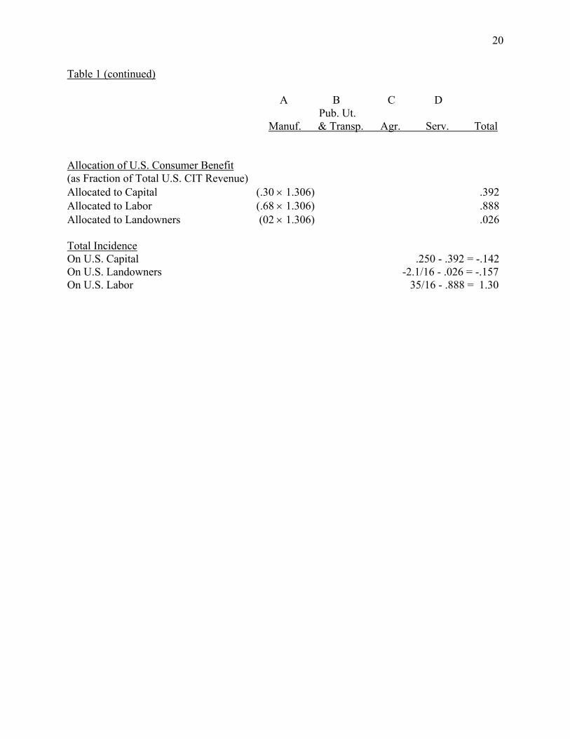
In panel 4 of the table we allocate this consumer benefit among U.S. factors of

production -- 30% to capital, 2% to landowners, and 68% to labor. There follows the final

calculation in which factor costs (+) are offset by allocated consumer benefits (-). The final

reckoning is net benefits to U.S. capital and to U.S. landowners, each equal to about 15% of U.S.

CIT revenues, together with a cost to U.S. workers equal to 130% of those revenues.6

Differentiated Products in Manufacturing

Clearly, the most natural candidate for our next step of modification is the assumption

that domestic and foreign manufactures are homogeneous products. Such an assumption is

plausible for agriculture, fishing and mining, but certainly not for manufacturing. Hence in this

section we will pursue the idea that some part of the tax wedge will be reflected in a rise in pa

relative to ,*ap the external price level of manufactures. For simplicity, I will stick with the

assumption that capital, worldwide, bears the full burden of the tax, so we will still have the rate

of return falling from 9% to 8% as a consequence of the tax. So we are again dealing with a

wedge equal to 7/8 of CIT receipts from the manufacturing sector. Earlier we had all of this

being reflected in reduced wage levels. Now, let us say only 4/8 is so reflected, with the

remaining 3/8 representing a “new” burden on consumers of U.S. manufactures. Table 2

presents this revised scenario.

6Our methodology does not include “excess burden” as a part of incidence. I always have liked the distinction between “burden” (an incidence problem) and “excess burden” (efficiency problem). Mathematically, “burden” can be treated (as we do here) as a first-order effect (ΣFjdpj, with F standing for factors), and “excess burden” as a second order effect, such

as j2

1ΣdFjdpj. Anyway, readers should realize that the measures of “burden” presented here are

intended to exclude “excess burden”.

23

TABLE 2

Illustrative Incidence Exercise Assuming

Manufactured Products Differentiated --

Other Assumptions Follow Table 1

A B C D Pub. Ut. Manuf. & Transp. Agr. Serv. Total

U.S. Reproducible Capital Income 25% 25% 0% 50% 100% (% Dist.) Share of Sectoral CIT Receipts Borne 1/8 1/8 - - by Capital in Sector Share of Total CIT Receipts Borne By 1/16 1/16 - 1/8 4/1 Capital in Sector U.S. Labor Income (% Dist.) 20% 10% 6% 64% 100% Share of Sector CIT Receipts Borne 4/8 2/8 By Labor in Sector Share of Total CIT Receipts Borne By 4/16 2/16 1.2/16 3.2×4/16 16/20 Labor in Sector U.S. Consumer Benefits Rising Price of Manufactures -(8/16 - 1/16 - 4/16) -3/16 Rising Price of PUT -(8/16 - 1/16 - 2/16) -5/16 Falling Price of Services From Lower Rate of Return 1/8 From Lower Wage 3.2×4/16 Total Consumer Benefit -8/16 .925 425.0

24

Table 2 (continued) A B C D Pub. Ut. Manuf. & Transp. Agr. Serv. Total

Allocation of U.S. Consumer Benefit (as Fraction of Total U.S. CIT Revenue) Allocated to Capital (.30 × 0.425) .1275 Allocated to Labor (.68 × 0.425) .2890 Allocated to Landowners (02 × 0.425) .0085 Total Incidence On U.S. Capital .250 - .1275 = .1175 On U.S. Landowners -1.2/16 - .0085 = -.0835 On U.S. Labor 20/16 - .289 = .961

25

The burden on capital as a factor remains in this scenario the same as before: U.S.

capital bears 1/4 of the burden; worldwide capital bears exactly the full burden. But now wages

fall less, because the prices of manufactured goods can (and do) rise. The specific reduction in

wages embodied in Table 2 is 4/7 the size of that in Table 1. Hence the burden on labor as a

factor ends up at 20/16 rather than 35/16 of total U.S. CIT revenues.

But in the final calculation labor’s burden does not fall quite so sharply. This is because

labor suffers over 2/3 of the extra consumer cost, entailed in the rising price level of U.S.

manufactures. Thus, in the end, labor ends up with a total burden (as factor and as consumers)

equal to .961 of U.S. CIT revenues, as compared with 1.306 in Table 1. U.S. capital shifts from

being a beneficiary to the tune of some 14% of CIT receipts, to bearing a net (factor cum

consumer) burden of about 12% of CIT revenues. The two factors -- U.S. labor and U.S. capital

-- thus bear 108% of CIT receipts, with the extra 8% going to U.S. landowners in their combined

factor/consumer roles.

I find these two scenarios to yield results that are close enough to each other to lead to

reasonably robust conclusions. U.S. labor bears “around” 100% of the burden of the U.S. CIT,

leaning above it as the passthrough of the tax to consumers of U.S. manufactures gets smaller.

Capital bears a small positive burden with passthrough, and gains a small positive benefit

without the passthrough. Landowners pick up a benefit to offset the degree to which labor and

capital together bear more than 100% of the burden.

Altogether, it seems that in any scenario fitting the general template of Tables 1 and 2,

U.S. labor and U.S. capital must bear somewhat more than 100% of the burden in their combined

factor/consumer roles. Why? Because farmers seem bound to gain as long as there is any net

26

consumer benefit. And if the net outcome for the farmers is positive, that extra burden must also

fall on U.S. labor and capital.

Why Not A Fuller Passthrough of the Tax Via Rising Prices of U.S. Manufactures?

This is a pretty easy question to answer, but it requires opening a door that we have

luckily been able to keep closed until now. The right way to look at the equilibria of Tables 1

and 2 is to consider them as post-tax phenomena. What we call CIT revenues is the tax rate

applied to ,'bK'

aK + the primes representing values in the with-tax situation.7

If we now assume no reduction in the rate of return and no reduction in U.S. wage rates,

we would have all the burden passed to U.S. consumers, whether of manufactures or of PUT. To

see what is wrong under this scenario, one must consider the incentives for capital to move out

of the U.S., and the incentives for foreign economies to absorb that capital. In both

manufacturing and PUT, we would have a double incentive to use less capital -- as product

prices would have risen to reflect the tax, so scale would be lower because of reduced demand.

In addition, factor substitutions would occur because the cost of capital would have risen (by the

amount of the tax) relative to that of labor. This ejected capital would go to the services sector,

and abroad. Furthermore, the amount sent abroad must equal the amount foreign economies

want to accept (according to their factor-demand relationships). The bottom line is that neither

U.S. services nor foreign economies will demand these funds unless the equilibrium rate of

return goes down.

7A nuance concerning Tables 1 and 2. Since they are counting only the capital stock that remains in the U.S. in the presence of the tax, they leave out of account the reduction net yield (from 9% to 8% in my example), on the capital that relocated abroad in the presence of the tax. This would add somewhat to the burden on U.S. capital owners, but it would qualify as a second order effect, dKf dpk where dKf is U.S. capital shifted abroad as a result of the tax.

27

Note on the Paper by Gravelle and Smetters

This is a good point for me to comply with the organizers’ wish that I comment

specifically on a recent paper by Gravelle and Smetters.8 Broadly speaking, I see this paper

almost as a natural extension of my 1995 paper, in that it employs the same 4-sector breakdown,

treats the CIT as a partial factor tax striking the earnings of capital in just two of those sectors,

and employs the “trick” of having land as an important factor (separate from reproducible

capital) in the agricultural sector. It goes well beyond my paper in introducing implicit

parametric demand and production formations both at home and abroad. I can only applaud

these additional developments.9

I am troubled not at all by the modeling per se, but rather by the parameter values that are

displayed in the tables. Let me say at the outset that I am not particularly worried about Cobb-

Douglas production functions or about sectoral demands based on a Cobb-Douglas function. But

if I were to modify these assumptions (implying substitution elasticities of -1), my inclination

would be to consider -1/2 as a first alternative. (For big sectors like food, rises in sectoral prices

8Jane Gravelle and Kent Smetters, “Who Bears the Burden of the Corporate Tax in the Open Economy,” Cambridge: National Bureau of Economic Research, May 2001 (NBER Working Paper 8280).

9In self defense, however, I must say that there is nothing unrigorous about solutions to the incidence problem that are based on price-formation equations, at least so long as one is willing to employ the assumptions of competitive behavior plus production functions that are homogeneous of degree one. These assumptions are fully sufficient in the small-country case (the country being a price-taker in both the capital market and the markets for tradable goods). These assumptions do not go all the way in the cases where world rates of return change as a result of the tax, nor in the case where tradable products are differentiated. But they can be made to give simple and straightforward answers to scenarios in which specific changes in world rates of return, and specific degrees of passthrough of the CIT into manufactured goods prices are explored. This is what I do in the present paper.

28

lead to a larger fraction of income being spent on the sector’s goods. Among factors, a doubling

of the cost of labor would in most cases lead to a larger fraction of expenditures going to labor,

and similarly for capital.)

My biggest objection, as already noted, concerns what the authors call the portfolio-

substitution or capital-substitution elasticities. This represents the responsiveness of capital

owners to differentials in rates of return at home and abroad. At issue here is how one looks at

the international capital market. The authors cite Feldstein and Horioka (1980), who highlight

the high correlation between national rates of saving and of investment. Nothing is wrong with

their correlations, but, as I noted long ago,10 they refer to gross saving and gross investment.

Once the depreciation component that is mathematically common to both is eliminated, the

resulting correlation between national rates of net saving and net investment is much lower. But

basically neither of these correlations is evidence of market imperfections. What is needed here

is data on relative rates of return. I like to think of the world capital markets as an interconnected

hydraulic network. One does not need perfect connections in all market segments in order to

effectively equalize rates (among the major advanced-country markets); one only needs a

sufficient number of active players in the markets where the pipes are fully open and where the

flows are massive and highly responsive to small differentials. This is what I think I see in the

world of covered interest arbitrage by major financial institutions. It is why I want to stick only

with the highest of Gravelle’s and Smetter’s portfolio elasticities.

10See Martin Feldstein and Charles Horioka, “Domestic Savings and Capital Flows,” Economic Journal, 90 (June 1980): 314-329 and Harberger, “Vignettes on the World Capital Market,” American Economic Review, 70 No. 1 (May 1980): 331-339.

29

The other elasticity that troubles me is the one between domestic and foreign

manufactured products. My instinct is to think of pairwise comparisons -- Ford versus Toyota,

Philips vs. Zenith, Exxon versus British Petroleum. What would happen, I ask, if one of these

raised its prices by 50 to 100 percent vis-a-vis the other? My economist’s bones tell me that

couldn’t really happen. Yet an elasticity of substitution of -3 implies an average own-price

elasticity of -1 1/2 which in turn implies huge market power.11

Once I narrow down Gravelle’s and Smetter’s tables to what I feel is a plausible range of

parameters, I get domestic labor bearing between 38 and 71 percent of the burden, and domestic

capital bearing between 55 and 36 percent of the burden with a presumption toward the 71/36

extreme (See their Table 2, rows 6 and 9.).

Compare this 71/36 extreme with my 96/12 result (my Table 2). These could easily

belong to the same family. Even more so when one considers that the Gravelle-Smetters

measure includes excess burden while mine does not, and that their measure probably includes

the loss (from reduced rate of return) that U.S. capital owners sustain on the capital that they

shift abroad as a result of the tax.

11Consider two sets of goods A and B where outside substitutes are negligible. If the elasticity of substitution between A and B is γab, let us write dlog A - dlog B = γab (dlog pa-dlog pb). Set dlog pb equal to zero and you get dlog A/dlog pa - dlog B/dlog pa = γab. Thus

.ab*ba

*aa γ=η−η Similarly, setting dlog pa equal to zero we get .ab

*ab

*bb γ=η−η Outside

substitutes negligible means relative quantities A/B respond only to the relative price pA/pB.

This leads to *ba

*bb η≡η and .*

ab*aa η−=η Substituting, we get

ab*bb

*aa γ=η+η

i.e., the elasticity of substitution is the sum of the two own-price elasticities (asterisks represent substitution-effect-only elasticities.)

30

So I think our results are pretty close to one another, once somewhat comparable

assumptions are imposed.

On other matters, I hope I can persuade Gravelle and Smetters to join my crusade for

clarity of concept. Statements like “the original Harberger (1962) argument that the incidence is

borne mainly by capital is now dead among academics” should be accompanied by the warning

that, if so, these academics have to understand that the choice between an open and a closed

economy is a matter of scenarios, not of reality. I’m sure that most academics would agree that

the closed economy result (that 100% borne by capital is in the middle, not at the extreme, of the

plausible range of outcomes) is the one that would apply in the case of a general worldwide

increase or reduction in the rate of corporation income taxation, and that the closed-economy

model is the right one to use in this case. Likewise, I hope that most academics would agree that

the open economy model is the right one to use if one country alone changes its CIT rate. And at

the same time they should agree that the circumstances of the two scenarios are sufficiently

different that there is no presumption whatever that we can make generalizations about incidence

that would apply equally well, regardless of whether a tax change was being implemented by one

country alone or by all countries simultaneously. The key is to use an analytical framework that

is appropriate for the scenario that one is exploring.

Notes On Short-Run, Transitional and Dynamic Incidence

This is a good topic with which to conclude this paper, because it brings us sharply back

to the opening theme, especially to the unknown and unknowable parts of that theme. To start

with something relatively simple, let us take the topic of short-run incidence. Here the idea has

always been that the owners or shareholders of an enterprise: a) have holdings of a set of assets

that represent fixed factors in the short-run, and b) are the residual claimants to the financial

31

flows generated by that enterprise. These two characteristics in turn pretty much guarantee that

they will initially bear the incidence of a new tax wedge.

But how long will this last? There is now a disequilibrium between the rate of return to

capital in the taxed sectors, and that in the rest of the market. The capital stock will end up

reallocated so as to once again equalize rates of return between the taxed and nontaxed sectors.

As this happens, rates of return will presumably go down in the nontaxed sector and up in the

taxed sector. Can we say anything about how long such a process will take? I think we can say

very little. Adjustment will be faster, the higher the rate of depreciation in a taxed industry and

the more readily saleable are its capital assets. But adjustment will also be faster, the smaller is

the size of the tax change in question. For with a tiny tax change, the needed adjustment of the

capital stock might turn out to be possible almost instantaneously, and without any extra cost. In

such a case we might jump to the long-run equilibrium solution in a single period, whereas with

a big tax wedge, a slow depreciation rate, and “implanted” (unsaleable) capital assets, it might

take ten years to reach the long-run solution.

All this makes me want to say that the details of such a transition process are pretty close

to unknowable. We can build models of the usual kind, with parameters in orders of magnitude

that we consider plausible, to get answers to the question of long-run incidence. But when we

have to add dynamics to such a model, I don’t think we can pin down the parameters of the

dynamic process into a range that is narrow enough for us to learn much (if anything) from the

exercise. I don’t need a dynamic model to reach the judgment that rate-of-return equalization

will not happen in one or two years (for a big tax wedge) and is pretty sure to have happened by

ten or twelve years. But do I think that a research project could be designed that would convince

32

me that yes, the adjustment will take place in 4 or 5 years, but almost certainly it will not take as

long as 6 or 7 years? No way!!!

* * * *

Happily, we can do somewhat better on dynamic incidence than on the transition

problem, but even here it takes a strong assumption to get easy answers. That assumption is that

the time path of the total relevant capital stock (within the total closed or open economy) is

going to be the same, with or without the tax. Then we can say that once equilibrium is reached

(i.e., once the transition is complete), we can think of a rolling equilibrium in a growing

economy. In such a rolling equilibrium, the net-of-tax returns in all sectors would be

continuously “equalized” (with due adjustments for risk, etc.), and goods and factor markets

would be continuously cleared. In short, our dynamic picture would be a set of images, each of

which would come from our standard comparative static model, only with a progressively larger

capital stock and labor force, and a progressively more advanced technology, year-by-year as we

modeled the passage of time.

I see no real problems with this; its only potential weakness seems to be the assumption

that the time path of tK is independent of the tax. This is an assumption that I personally find

quite easy to live with. My own experience with high-real rates of return (up to 3% real per

month on bank deposits, up to 20% real per year on Central Bank bonds) in Latin America leads

me to the conclusion that ordinary people do not modify their consumption/saving decisions very

significantly in response to higher yields. (This does deny that the allocation of given savings

among asset groups is responsive to differences in yield. It also, correctly for this purpose,

defines savings in a national-income sense, excluding capital gains and losses on existing assets.)

So with this assumption we can say we have a pretty good sense of what a rolling dynamic

33

equilibrium looks like. But of course this is just a modest extension of the results we have been

getting from comparative-static models for half a century.

* * * *

Once we release the assumption that the time path of the total capital stock is

independent of the tax we are analyzing, all bets are off. Now everything depends on the

dynamic mechanism by which total saving responds, which is something about which I neither

see nor foresee any professional consensus for a long time to come.

Here I think our best bet is to make the most of what we know, and leave in limbo the

remaining questions. To put some flesh on the bones of this argument, let me pose the question

of the incidence of the corporation income tax in the U.S. I am ready to assume that the time

path of the world capital stock was independent of the time path of U.S. and other corporation

tax rates. So for me the incidence problem seems manageable. But for someone else who isn’t

ready to go along with this key assumption, I would suggest posing the question the following

way. Suppose the world capital stock were frozen at today’s level, and certain changes in one or

more CIT rates were implemented. What would be the efficiency and incidence consequences,

as this given capital stock was reallocated so as once again to “equalize” rates of return and to

clear all markets? The answer to this question may not be the final answer to these people, but I

think it would be a good start.

One could then ask them to project, for the future, a time path of tK with no change in

rates, and another for tK with the changes we are analyzing. The easy case here would be one

in which the equilibrium rate of growth was the same, with and without the tax changes, and in

which, then, the time path of total capital with the tax changes ended up being year by year, a

certain fraction of its time path without the tax changes. This would permit us to replicate the

34

rolling equilibrium based on the assumption that tK is independent, with an alternative rolling

equilibrium in which the new tK is simply β times the old one. Incidence for any period could

then be derivable from our old, user-friendly, comparative-static models.

But in the end, the whole story of dynamic incidence depends on what we are prepared to

assume about saving behavior. I’m afraid that whatever is assumed here is bound, for a long

time to come, to have a huge Bayesian component. The idea that we will somehow stumble

upon evidence that will lead to a general professional consensus regarding the responsiveness of

saving to rates of return -- that idea is to me just a dream.

Summary and Conclusions

(1) The world never gives us a “clean” incidence scenario in which we can trace out the

consequences of a tax change by simply following the data. I believe incidence exercises will

always be “in our heads” as we insert tax changes into models that we think adequately represent

the real world in its main relevant aspects.

(2) If we want to answer a really “real-world” question, we have to think of inserting

“our” tax change into a setup in which we clearly specify how the proceeds are likely to be spent

(or used to reduce other taxes), and what other distortions will be present as our incidence

scenario is played out. It is clear that without such a specification the pattern of response could

be almost anything -- i.e., would reasonably be called unknowable.

(3) If we want to answer the standard “academic” question of what is the incidence of

the corporation income tax, we have to think of creating clear scenarios in terms of which such a

question makes sense. The traditional wisdom has been that we should insert “our” tax into a

scenario with no other distortions and under an assumption of demand neutrality.

35

(4) Even when we do this, we have to sharply distinguish between a closed-economy

scenario (where all major countries insert, raise or lower a corporation income tax) and an open-

economy scenario in which just one or only a few countries do so. Note that, thinking of the real

world, I do not talk about a single country as being a closed economy. But the world as a whole,

of course, is one.

(5) I felt uncomfortable with my own analysis of the open economy case until I came

upon the notion of a 4-sector model, with manufacturing, public-utilities and transport,

agriculture and services representing the four possible combinations of corporate/noncorporate

and tradable/nontradable.

(6) I make a major point of the wisdom of building models in which rates of return are

“equalized” around the world. For a small economy this means that its country risk premium

will be no different “with” or “without” its CIT. For a large modern economy like the U.S. it

means that any change in its rate of return (induced by its CIT) will be shared with the rest of the

world.

(7) This assumption, plus that of the small country being a price-taker in product markets

for tradable goods practically guarantees that labor (in its role as a factor of production), will

bear more than the full burden of the corporation income tax in a small country. In their roles as

consumers, labor and capital would gain somewhat, but labor still would end up bearing more

than the full CIT burden.

(8) The example of Table 1 shows labor bearing somewhat more than the full burden of

the CIT in an economy that looks something like the U.S., where at the same time the same full

burden is also precisely borne (by design of the Table) by the owners of capital throughout the

36

world. There is no double-counting here. Foreign labor gains at the expense of foreign capital,

and U.S. consumers and landowners gain at the expense of U.S. labor.

(9) Table 2 incorporates the realistic possibility that the country is not a complete price-

taker for manufactured goods. It allows close to half of the burden of the CIT paid in that sector

to be pushed forward to consumers of manufactured products. This changes the final incidence

picture derived from Table 1. Instead of labor ending up bearing (as factor and consumers)

130% of the burden of the CIT, it now ends up with 96% of the burden. Again, worldwide

capital, by construction, bears 100% of the CIT burden.

(10) No example is given with consumers of manufactures bearing the full weight of the

CIT paid by that sector, because I consider that extreme case to be unrealistic. Some important

ejection of capital from the corporate sector is virtually inevitable. If there is any passthrough

via higher prices to consumers, demand for capital will fall in both the tradable and nontradable

corporate sectors, from both a scale effect and a substitution effect. This capital will have to be

absorbed by the rest of the world plus the local nontradable sectors, entailing a fall in the rate of

return to capital there.

(11) In brief comments on the paper by Gravelle and Smetters, I have nothing but praise

for their two-region, four sector model as such, but have serious problems with two of their key

parametric judgments. The most important of these concerns the workings of the international

capital market. I find it quite implausible that relative real rates of return would change, as

between, say, Europe and the U.S., as a consequence of a change in the U.S. CIT. On the other

problematic parameter, I believe that although product differentiation permits differential

movements of manufactured goods prices between, say, the U.S. and Europe, a high degree of

substitutability nonetheless prevails. All this leads to my feeling quite easy with the results that

37

they get under their highest assumptions regarding substitutability in the capital and

manufactured-goods markets, but uneasy with their lower-substitutability cases.

(12) Unfortunately, their own generalizations about their results focus on U.S. capital

bearing close to the full burden and U.S. labor bearing little. These generalizations come from

parts of their tables that assume relatively low substitutability in the capital and manufactured-

goods markets.

(13) On the subject of short-run and transitional incidence, I find the idea of the

immediate impact being borne by the immediate residual claimants (equity owners) to be quite

acceptable, but it doesn’t teach us much. It by definition creates a capital-market disequilibrium

which will presumably be resolved over time. I believe that the time path of this resolution (the

transition) belongs in the class of the unknowable.

(14) Dynamic incidence is somewhat more tractable. If one is ready to consider the time

path of the total capital stock to be independent of the tax, dynamic incidence can be derived

from a rolling equilibrium of the comparative static model, with growing stocks of labor and

capital and with steadily improving technology. With endogenous savings, a significant subclass

of models would lead to an equilibrium “with” the CIT characterized by a given K/L ratio, and

to an equilibrium “without” the CIT involving a lower K/L ratio. At any given point in time,

then, one would solve the incidence problem by imposing a “with tax” equilibrium capital stock

that was, say, β times that stock in the “without tax” situation.

If, however, we want dynamic results based on solid knowledge about people’s saving

behavior, I think we would have to use the term unknown, if not unknowable.