1

Core Descriptions, Core Photographs, Physical Property Logsand Surface Textural Data of Sediment Cores Recovered fromthe Continental Shelf of the Monterey Bay National MarineSanctuary During the Research Cruises M-1-95-MB, P-2-95-MBand P-1-97-MB

By Kevin M. Orzech, Wendy E. Dahl, and Brian D. Edwards

U.S. Geological Survey345 Middlefield Rd., MS-999Menlo Park, CA 94025

Open File Report 01-107

2001

This report is preliminary and has not been reviewed for conformity with U.S. GeologicalSurvey editorial standards or with the North American Stratigraphic Code. Any use oftrade, product, or firm names is for descriptive purposes only and does not implyendorsements by the U.S. Government.

2

Linked Table of Contents

Introduction ........................................................................................... 3

Acknowledgements .................................................................................. 4

Sample Collection Procedures ...................................................................... 4

Box Corer ............................................................................................ 4

Piston Subsampling System ...................................................................... 5

MultiCorer™ ........................................................................................ 6

Grab Sampler ....................................................................................... 7

Analyses of Subcores ................................................................................. 8

Surface Texture ..................................................................................... 8

Multi-Sensor Logging of Physical Properties ................................................. 9

Splitting and Core Handling ................................................................... 12

Digital Photography and Image Processing ................................................. 13

Visual Descriptions .............................................................................. 13

Data Editing and File Management ........................................................... 14

Spreadsheet of Station Data ....................................................................... 14

Web Navigation ...................................................................................... 16

Web Browser Tools .............................................................................. 17

Adobe®Acrobat® Tools ........................................................................ 17

More Navigation Tips ........................................................................... 19

References ............................................................................................ 20

Results ................................................................................................. 20

Spreadsheet of Station Data (416 kb) ............................................... linked file

Index Map (608 kb) ..................................................................... linked file

Surface Texture Map (172 kb) ........................................................ linked file

Table 1 and 2 .......................................................................................... 21

For additional information, contact the corresponding author:Dr. Brian D. EdwardsU.S. Geological Survey345 Middlefield Road, MS-999Menlo Park, CA 94025650.329.5488 deskbedwards@usgs.gov

3

Introduction

In response to the 1992 creation of the Monterey Bay National Marine Sanctuary(MBNMS), the United States Geological Survey (USGS) initiated a multiyearinvestigation of the Sanctuary continental margin. As part of the investigative effort, thisreport summarizes the shipboard procedures, subsequent laboratory analyses, and dataresults from three seafloor sampling cruises conducted on the continental shelf betweenthe Monterey peninsula, CA, and San Francisco, CA (fig. 1). The cruises were conductedin 1995 aboard the NOAA Ship McArthur (M-1-95-MB) and in 1995 and 1997 aboardthe R/V Point Sur (P-2-95-MB and P-1-97-MB). Scientists and representatives from theEnvironmental Protection Agency (EPA), the National Oceanic and AtmosphericAdministration (NOAA), the California Department of Fish and Game (CDFG), theUniversity of California Santa Cruz (UCSC), and the San Jose State University MossLanding Marine Laboratory (SJSU-MLML) supported the research effort.

Figure 1. Map showing sample locations and the study region bounded by theshoreline, the shelf break, and the north boundary of the sanctuary.

Three hundred and eighty four stations were occupied during the study. Of these,342 stations were predetermined based on a horizontally stratified, randomized samplingdesign following the Environmental Protection Agency EMAP protocol (Overton et al.,1990; Stevens and Olsen, 1991; White et al., 1992). The remaining 42 stations were

4

chosen either to sample specific geological targets or to occupy gaps in the randomizeddesign. Ship positioning was determined by differential GPS (accuracy +/- 10 m); corestypically are obtained within 50 m of the predetermined sampling location. Water depthat the time of sampling was determined by use of a 12-kHz acoustic profiler. On thevarious cruises, either a 1.5-10 kHz Data Sonics Chirp or a 3.5-kHz seismic-reflectionprofiling system was used to examine and document the local acoustic stratigraphy ateach sampling site.

In this report we present sediment descriptions, sediment textural data, physicalproperty logs, station metadata, and photographs of subcores from box cores andMultiCores™ collected during the cruises. The report is presented in an interactive web-based format accessible with Adobe®Acrobat® downloaded free at this URL:

http://www.adobe.com/prodindex/acrobat/readstep.html

Acknowledgements

The authors thank the many scientists, students, and technicians involved in thecore collection and sampling program, as well as the capable officers and crews of theNOAA Ship McArthur and the R/V Point Sur (Moss Landing Marine Laboratory, SanJose State University). We also thank H.E. Clifton, J.V. Gardner, and R.L Phillips for theinsights they provided with regard to core description and interpretation. D. Ponti createdthe FileMaker™ Pro5 database that allowed for easy organization of the core descriptionlayouts. M. Medrano and J. Stocking-Albizo performed the textural analyses of thesurface sediment. A review by H.J. Lee improved the final version of this Open FileReport. This research was funded by the U.S. Geological Survey Monterey Bay NationalMarine Sanctuary project.

Sample Collection Procedures

A box corer, a MultiCorer™ and a grab sampler were used to obtain sedimentsamples from the continental shelf. Brief descriptions of the three devices and thecollection procedures follow. Two tables at the end of this document list the type ofsubsamples taken from the sediment recovered from each coring device and the scientistin charge of that sampling procedure ( link to table 1 and 2 ).

Box Corer

Bottom sampling was accomplished primarily by use of the Naval ElectronicsLaboratory (NEL) – style spade box corer equipped with a removable box (fig. 2). Thecorer weighs approximately 1500 lbs in air. Immediately prior to sampling, a 35-mmbottom-trip camera system with strobe light photographs the segment of the seafloorbeneath the box corer (these photos are available for viewing through the correspondingauthor). The corer then recovers a nearly undisturbed 0.06 m2 sample (20 X 30 cm) up to60 cm in length. Early attempts with a larger format (40-cm X 40-cm X 60-cm) corerwere abandoned in favor of the smaller box corer.

Following coring, the corer is returned to the ship’s deck, the box is detached and thesupernatant seawater is siphoned away from the surface of the sample. The quality of thesurface is recorded, and typically a photograph is taken of the core surface.

5

Figure 2. NEL-style Spade Box Corer

Piston Subcoring System and Subsampling.

The removable box containing the core sample is then placed inside a framedesigned to push polybuterate tubes (8.5-cm diameter) into the sediment using a lineractuator (fig. 3A). The tubes, fitted with a fixed piston, thereby recover a nearlyundisturbed subcore of the main sample (fig. 3B).

A B

Figure 3A and B. USGS-designed piston subcoring system. A) Subcoring framebeneath linear actuator. B) Subcore and piston apparatuses positioned for subsampling.

6

Surface samples are then taken (e.g., for texture or microfauna) (fig. 3C), the boxfaceplate detached, and the subcores removed (fig. 3D). Typically, the remaining bulksediment is then washed through nested sieves to capture macrofauna.

C D

Figure 3C and D. C) Schematic diagram looking down at the top of the sample showingtypical subsampling scheme. D) Deck photograph showing box with subcores inserted,and faceplate removed.

MultiCorer™

In addition to the NEL-style Box Corer, a General Oceanics MultiCorer™ (figs. 4Aand 4B) was used during cruise P-2-95-MB aboard the R/V Point Sur.

A B

Figure 4A and B. A). General Oceanics MultiCorer™ being lowered to the deck afterrecovering samples. B). Detail photograph showing recovered sediment.

7

The corer, equipped with cast-acetate tubes, is designed to recover up to eight nearlyundisturbed samples simultaneously (fig. 4C). The system is designed to recover anominal maximum of 45 cm of sediment in each 10.1-cm diameter and 75-cm long tubethereby allowing 30 cm of tube volume for supernatant seawater to protect the sedimentsurface. Each tube is individually sealed with top and bottom caps resulting in anexceptionally high quality sediment-water interface (figs. 4B and 4D).

C D

Figure 4C and D. C) Schematic of subcores recovered by the MultiCorer™. D) Bottomphotograph taken at the time of sampling. Shows base caps moving to seal the tubes asthe corer is being extracted from the seafloor.

Although the MultiCorer™ recovered samples of excellent quality, operationaldifficulties in holding position above the corer in shallow water resulted in bending andtorquing the corer frame and damaging some of the acetate subcore tubes. Accordingly,we stopped using the MultiCorer™ midway through the cruise P-2-95-MB.

Grab Sampler

At sites where high-resolution seismic-reflection geophysics indicated a thinlysedimented, hard, or rocky bottom, a Van Veen–style grab sampler was used to evaluatethe bottom type prior to using one of the higher quality (and more fragile and expensive)coring devices (fig. 5). In many cases, these grab samples were the only samplesrecovered at the site.

8

A B

Figure 5. A) Grab sampler being recovered. B) Grab sampler being subsampled.

Analyses of Subcores

Selected subcores from each box core and MultiCore™ station were run through asequence of laboratory procedures that consisted of: 1) non-destructively logging forphysical properties, 2) splitting the subcore longitudinally into working and archivehalves, 3) photographically documenting the split subcore, 4) describing the visualcharacter and color of the subcore, and 5) taking samples for laboratory analyses. Thirty-one selected subcores were X-rayed to reveal internal physical and/or biogenicallyproduced structures. The X-ray radiographs are not included in this report, but can beviewed by contacting the corresponding author .

Surface Textural Analysis

Edwards (in press) measured the surface texture at most coring stations fromsamples taken from the tops of the box cores and MultiCores™. The results arepresented numerically on the Spreadsheet of Station Data (416 kb) (table 3) and spatiallyon the Surface Texture Map (172 kb) (fig. 6).

The detailed textural analyses were preformed on the top 1 to 2-cm of recoveredsediment. The analyses were done in the lab following a standard grain size multiple stepprocedure that yields measurements in half phi intervals. Each sample was run throughthe procedure described below.

First, hydrogen peroxide was added to a sample to remove organic matter. Thehydrogen peroxide was then boiled off. Salts were removed by washing the samples withdistilled water, centrifuging, and then decanting the water. Next, the sample wassegregated into gravel, sand and mud (silt and clay) fractions by washing throughstandard 1-mm (-1 phi) and 63-micron (3.5 phi) sized sieves. The gravel and sand weredried and weighed. The sand was then run through a USGS-designed rapid sedimentanalyzer (RSA). The RSA is a 2-m-long water-filled tube that generates grain size valuesin 0.5 phi intervals using the principles of Stokes Law.

The fine fraction (<62 µm) was placed into a beaker, disaggregated with sodiumhetamexaphosphate (Calgon solution) and left to sit overnight before a representativesample (aliquot) was taken. The aliquot was run through a Micromeretics™ SediGraph

9

which determines grain size of the mud fraction by using a laser that measures thechanges in water clarity that correlate with particle settling.

The total amounts within all half-phi-sized increments of gravel, sand and mudwere then entered into a USGS-developed statistical program called SedSize. SedSizegenerated weight percent values in half phi intervals. These values are displayed on theSpreadsheet of Station Data (416 kb) (table 3).

Multi-Sensor Logging of Physical Properties

Compressional-wave (P-wave) velocity, wet bulk density and magneticsusceptibility of the subcores were measured in shipboard laboratories using theSchultheiss Geotek Multi-Sensor Logger™ (MSL) system (fig. 7). Measurements weremade on-board ship because P-wave velocity and wet bulk density are state propertiesthat typically change with time and storage. The logging system is described in detail inKayen et al. (1999), Gardner et al. (1995), Kayen (1994) and Cowen et al. (1994). Thefollowing description is exerpted from those reports.

The MSL-system consists of a 4-m-long tracking system and three sequentialmeasurement devices: 1) a compressional-wave (P-wave) velocity and core-diametersensor, 2) a gamma ray attenuation porosity evaluator (GRAPE), and 3) a magnetic-susceptibility sensor. The system is controlled by a Macintosh SE/30 driven byacquisition software written as a HyperCard© stack (Kayen and Phi, 1997). Whole coresections up to 1.5 m in length can be logged with the MSL-system.

Movement along the tracking system is run by a computer-controlled steppermotor that advances the core section at a selectable interval set to 1-cm during logging.Each core section was run consecutively through the sensors, starting with the top(sediment surface) section and progressing through to the bottom of the core. Sixteen ofthe cores were not logged and have no MSL data.

Figure 7A. Plan view of the Multi-Sensor Logger.

10

Figure 7B. Photograph of the detectors and sensors at the heart of the MSL systemshowing the calibration core completing a logging run from right to left.

Compressional-Wave Velocity Measurements

The compressional-wave velocity sensor is a two-component station. In additionto two sonic transducers, the station incorporates a very accurate ( + 0.1 mm) distancemeasuring sensor (LVDT) that measures the separation of the transducer heads and hencethe core diameter. The sensor measures the travel time of a 500-kHz compressional pulsesent through the medial-line of the core. Compressional-wave velocity is sensitive totemperature, so sediment temperature was measured just prior to and following thelogging of each core section.

Compressional-wave velocity of the sediment is calculated from the measuredcore diameter and travel time, with corrections for liner thickness, electronic-signaldelays, and core-liner travel time. The compressional-wave velocity (Vp) is calculatedas:

Vp = D-2L . T-2T

liner – T

electronics

where D is the whole core outer diameter, L is the liner thickness, T is the total traveltime, Tliner is the liner travel time, and Telectronics is the electronic delay within thetransducers, wiring, and electronics packages.

Wet Bulk Density Measurements

The Gamma-Ray Attenuation Porosity Evaluator (GRAPE) sensor uses a 137Cssolid-source capsule (12 milli-curies at delivery) to produce gamma rays at 0.662 MeV.The source capsule is housed in a lead shield and the core is exposed to a beam of gamma

11

rays emitted through a collimator hole in the lead shield (fig. 8). The collimator hole isabout 11-mm in diameter and 52-mm long. A lead-lined box was also placed over thesource and detector during logging for additional shielding. Gamma rays were detectedand counted by a Harshaw-type 6S6/1.5B NaI (TI) scintillation detector.

Figure 8. Detached and assembled views showing the construction and lead shieldingof the 137Cs source.

The number of gamma rays that pass through the core is detected during a definedtime interval. Sediment wet-bulk density can be determined with the following equation,which modifies Lambert’s Law to account for the influence of the core liner

ρb = {ln Io/I – 2L * ρliner * µ liner}

µsed(D-2L)

In the formula, D is the outside diameter of the core liner, L is the liner thickness, ρliner isthe liner density, µ liner is the liner Compton scattering coefficient, µ sed is the sedimentCompton scattering coefficient, I is the number of gamma ray counts that are detectedpassing through a core during a defined time interval, and Io is the number of counts thatpass through air during the defined time interval. µ sed and ρliner * µ liner are obtained bylogging water and aluminum standards, observing counts, and then backcalculating theneeded parameters.

Magnetic Susceptibility Measurements

The magnetic susceptibility of the sediment is measured directly by a 140 mm-diameter Bartington MS-2 transducer coil. This ring senses the magnetic susceptibilityaccurately for cores with sediment diameter up to about 91 mm. The box core subcoresand MultiCores™ have inside diameters of about 80 mm and 95 mm, respectively.Accordingly, every magnetic susceptibility reading made by the MS-2 system was

12

corrected using a compensation graph for different diameters given in the BartingtonManual.

All magnetic susceptibility readings are unitless and in the cgs system. Graphedvalues in this report are listed in whole numbers for convenience. They need to bemultiplied by 10-6 to obtain the correct value. Because the range of magneticsusceptibility values varied enormously throughout the study, three data ranges for theabscissa (0-100, 0-250 and 0-1000 * 10-6 cgs) were used. The magnetic susceptibilitygraphs in this report depict the smallest of these ranges that incorporates all magneticsusceptibility data for a core.

Splitting and Core Handling

After shipboard logging with the MSL system, the polybuterate subcores takenfrom the box cores were split lengthwise in an on-shore laboratory using a splitterpatterned after the Deep Sea Drilling Project design. The splitter uses a capstan and arope to pull a pair of utility blades down the length of the core (fig. 9). The blades cutonly the liner, not the sediment. The blades are mounted in housings on either side of thecore. The housings, attached to tracks by a set of bearings, are pulled along the outside ofa channel on which the core rests. Thus, the blades simultaneously slice opposing sidesof the core liner.

Figure 9. Finishing the splitting of a core liner with the splitter.

The core splitter was ineffective in cutting the hard, cast acetate MultiCore™liners . Accordingly, these liners were cut longitudinally by use of a table saw. Aftereither type of liner was cut, a tensioned wire was pulled through the sediment from top tobottom to yield two equal sized half cores – an archive and a working half (fig. 10).

13

A BFigure 10. A) Pulling a tensioned wire through a subcore. B) Exposed surfaces ofworking and archive halves of a subcore.

Digital Photography and Image Processing

Archive halves were placed on a core rack adjacent to a ruler and a Munsell SoilColor Chart. The rack was positioned on a photo stand under a Kodak™ ProfessionalDCS 620 digital camera with a Nikon™ 28-mm apochromatic lens. All images wereimported into Adobe®Photoshop® 5.5. Images were cropped to 30-cm increments inAdobe®Photoshop®. For cores longer than 30-cm, a 0 to 30 and a 30 to 60-cm imagewere meshed to yield a composite image of the whole core. These images contain thecolor charts and ruler so that they may be manipulated to obtain the true color of thesediment (the composite images are not included as part of this report but may beaccessed by contacting the corresponding author ). Next, the composite image wascropped to an image of the core sediment only. Brightness, sharpness and color balanceadjustments were made to this image with two primary goals: to obtain an accurate colorof the sediment and to enhance the visual features of the sediment. These final imagesare generally slightly lighter colored than the actual core sediment. Last, the images wereplaced into a FileMaker™ Pro5 database and are presented as part of this report.

Visual Descriptions

Visual descriptions were performed immediately after photographing the coreusing the working and archive halves side-by-side. Descriptions consisted of grain size,sorting, color, macro- and ichnofossil content, bioturbation intensity, lithologicaccessories and physical structures. A grain size estimate was determined for at leastevery 10-cm core interval by obtaining a small sample from the working half and using ahand lens with a grain size card that is delineated in half phi intervals. A simple visualsorting of the sediments was obtained by viewing the same sample with the lens and card.This visual sorting and grain size are not to be confused with the detailed surface texturaldata described above. Visual sorting was not determined for mud-rich sediments or formany of the first cores described (mostly the P-2-95-MB cruise). Sediment color wasdetermined by placing Munsell Soil Color Charts over the sediment and finding the bestmatch. Bioturbation intensity was assessed visually both after splitting and when thesediment surface was smoothed with a metal spatula. The degree of bioturbation wascatalogued under one of the following 5 categories: Abundant (>60% of the sedimentdisturbed by bioturbation), Common (30-60%), Moderate (10-30%), Rare (<10%), andNone Observed. Physical structures, macro- and ichnofossils, and lithologic accessorieswere also listed from visual assessment of the cores. X-ray radiographs for 31 coresprovided more details of structures and bioturbation.

14

After the cores were described, both halves were sealed with Handi-Wrap®,placed in plastic D-tubes and stored in a refrigerator that maintained temperaturesbetween 34˚ and 40˚ F. The reefer is at the USGS in Menlo Park, CA.

Data Editing and File Management

Raw MSL data for sixteen cores were recalculated because of poor calibration atthe time of logging. All MSL data was further editted by the following rules:

1) Discarded values fell outside of the range 1.3-2.2 g/cc for wet bulk density and 1.4-1.8 km/sec for P-wave velocity. No magnetic susceptibility values werediscarded.

2) If a density value was edited out, the velocity and magnetic susceptibility values ofthe same increment were also edited out regardless of their value.

3) When the last density, velocity or magnetics value of the core was abnormally lowcompared with the rest of the MSL data for the core, the datum was edited out.Values successively up-core from this bad datum were edited out following thesame procedure. Data was removed only from the lower 1 to 4 cm of core. Thesevalues were considered inaccurate and usually low because poorly consolidatedsediment or less sediment occupied the ends of cores.

The visual descriptions and editted MSL data were entered into theAppleCORE™ 8.1a program – a customizable core graphing program. During theprocess, this visual data was cross-checked for errors by comparing the digitalphotograph of the core with the data and visually reassessing any cores with questionabledata. Next, core photographs and AppleCORE™ layouts were imported into aFileMaker™ Pro5 database designed by the USGS. Within the database, the final corelayouts were assembled on one sheet by combining the AppleCORE™ layouts, photos, aborder and the proper headings of core and cruise I.D., latitude and longitude, waterdepth, and date sampled. Each of these files was saved as an Adobe®Acrobat® PDF fileand linked to the Index Map (608 kb) (fig. 11), Legend (fig. 12a and 12b) andSpreadsheet of Station Data (416 kb) (table 3) using Adobe®Acrobat® 4.05.

Spreadsheet of Station Data

The Spreadsheet of Station Data (416 kb) (table 3) catalogues all location, date,time, recovery, and sampling and surface textural data for each core station. AnAdobe®Acrobat® 4.0 version of the spreadsheet contains links to each core descriptionand photo sheet. To access the links click on the blue Station ID (core ID) numbers. Usethe back button to return to the spreadsheet. A Microsoft®Excel 98 version of the samespreadsheet is included in the report folder and linked to the Home Page so that the datamay be resorted and organized for the viewer’s needs. Use the spreadsheet headings keybelow to understanding the column headings of the Spreadsheet of Station Data (416 kb) (table 3). The heading bar on the spreadsheet links to this key:

CRUISE ID: Represents the cruise identification number for the sample station.

STATION ID: Sample station identification number, consistent with the linked coreidentification number on the Index Map (608 kb) (fig. 11). The first letter of thestation number represents the type of sampling device used at the station (B – Boxcorer, C – Grab sampler, and M - MultiCorer™).

JD/TIME (GMT) : Time and date of sampling expressed in Julian Day (JD)/GreenwichMean Time (GMT). The Julian day is expressed beginning with January 1st as

15

day 1 and December 31st as day 365 (366 during leap year). Greenwich MeanTime is the time at Greenwich, England located at 0.00 degrees longitude.

DEPTH (m): Depth in meters at the sample location.

REC.: Indicates whether or not a sample was recovered at the station.

LAT. and LONG. DD: Latitude and longitude of the station location in decimal degrees.

SURF. QUAL.: Indicates a sediment surface quality value that was recorded once thebox core was returned to the ship. Values are from 0 to 5, with 0 being thelowest value of quality. “No” shows that no value was recorded for the station.

REC. (cm): The length of the sediment sample recovered at the station. For box cores,this represents the height of the sediment in the box cores prior to subsampling.

SS: Indicates if a subcore was taken for stratigraphy and sedimentation studies.

SS (cm) : The length of the SS subcore. Occasionally the length of the SS subcore wasdifferent than the total recovery due to an uneven surface of the box core sedimentor air in the core liners.

SURF. TX .: Indicates whether a sample was taken for surface texture analyses.

MF SURF .: Indicates whether a surface sample was taken for microfauna studies.

MF CORE, GT, and GC: Indicates if a subcore was taken for microfauna, geotechnical,or geochemical studies, respectively.

TMSO: Indicates if a subcore was taken for chemical study of metals, pesticides, andPCBs.

MB: Indicates if macrobenthos subcores were taken. The table lists four MB columnsbecause up to four MB subcores were taken at individual stations.

MB WASH : Indicates if sediment in the box core was washed and sampled formacrobenthos studies.

MICRO. ORG.: Indicates if a 5-cm subcore sample was taken for micro-organismstudies.

PB: Indicates if a subcore was taken for lead-210 dating purposes.

BULK, OTHER SAMPLE: Indicates if bulk or other samples or subcores were taken.

CORE DES. AND PHOTO: Indicates if core descriptions and core photographs areavailable and linked to the index map of this report.

BOTTOM PHOTO: Indicates if a bottom photograph was taken at the sample station.

MSL DATA: Indicates if multi-sensor logger data were taken and are linked to the stationidentification number on the index map.

16

C14 SAMPLES and DIATOM SAMPLES: Indicates which cores were sub-sampled forcarbon-14 radiometric dating and diatom analyses.

GRAIN SIZE DATA: Indicates if detailed surface textural data was measured in the laband listed in the columns to the right of this column.

# OF SIZE CLASSES: Indicates the number of 0.5 phi-size classes represented in eachsurface textural sample.

COARSE SIZE LIMIT: Represents the coarsest phi-size grains of the surface texturalsample.

TOTAL WEIGHT OF SAMPLE (g): Shows the total weight in grams of the entire sampleused for grain size analysis.

-1.0, -0.5 ,…14.00: Shows the weight percents for each phi-size of the textural sample.

TOTAL 100%: Indicates the sum total of the phi-size weight percents (which ideally is100%).

% GRAVEL, SAND, SILT, CLAY and MUD: Represents the percentages of gravel, sand,silt, clay, and mud in each sample.

GRAVEL/SAND, SAND/SILT, SILT/CLAY, SAND/CLAY, SAND/MUD, andGRAVEL/MUD: Shows the ratios of the various size classes.

1 ST MOMENT (mean): Indicates the mean grain size of each sample.

VARIANCE: Shows a value representation of dispersion calculated as the sum of thesquared deviations from the mean grain size for each phi-size class divided by thenumber of phi-size classes with data.

STANDARD DEVIATION: Indicates the deviation from the mean. It is a value measureof dispersion calculated as the square root of the variance.

3 RD MOMENT : Measure of skewness - the asymmetry of the distribution (Carver, 1971).

4 TH MOMENT: Measure of kurtosis - how “humped” or “peaked” the central part of thedistribution appears (Carver, 1971).

COMMENTS: Provides any additional information for each sample station.

Web Navigation

On most computers, the open file report will open in the Adobe®Acrobat® 4.0program within your Internet browser. (It fails to do this when an Adobe®Acrobat® 4.0plug-in is not installed within the computer preferences. Installing the free plug-in(available at http://www.adobe.com/prodindex/acrobat/readstep.html ) or downloading theentire report onto your desktop will mitigate this problem). The Adobe®Acrobat®software and Internet browser tools will enable users to view all images and to link fromthe Index Map (608 kb) (fig. 11) or Spreadsheet of Station Data (416 kb) (table 3) to eachcore description sheet, the Surface Texture Map (172 kb) (fig. 6), the Home Page and thelinked Text and Table of Contents of this text document. Use and understanding of three

17

main browser tool buttons ( Back , Forward and Reload (Netscape Navigator™) orRefresh (Internet Explorer™)) and six main Adobe®Acrobat® buttons (the Hand Tool ,Zoom Tool , Go to Previous View , Go to Next View , Fit in View , and Find ) will enableyou to navigate smoothly through the report.

Web Browser Tools

The Back and Forward buttons on your browser tool bar (fig. 13) will take you toand from files that have been previously opened. Some browsers have run into theproblem of large files that fail to load or appear when a link is pressed. When thishappens without the appearance of an explanation window use the Reload button (fig. 13)in Netscape Navigator™ and the Refresh button in Internet Explorer™. The failure offiles to load occurs more commonly on computers with small memory particularly whenloading the Index Map.

Figure 13. Right side of the Netscape Navigator™ 4.08 tool bar.

Adobe®Acrobat® 4.0 Tools

Use the Adobe®Acrobat® tools (fig. 14) to access the links, to zoom in and out ofa page, to change the view size, to navigate within this text document, and to find keywords or numbers on a particular view. To navigate between the linked pages click on theHand Tool on the tool bar (fig. 14 and 15). The cursor will change to a hand. Onceplaced over a link, the hand changes to a hand with a pointing finger. Clicking on thelink at that time brings up the linked file.

Figure 14. Adobe®Acrobat®Reader4.0 tool bar.

18

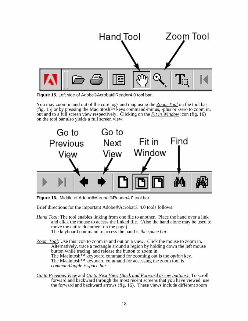
Figure 15. Left side of Adobe®Acrobat®Reader4.0 tool bar.

You may zoom in and out of the core logs and map using the Zoom Tool on the tool bar(fig. 15) or by pressing the Macintosh™ keys command-minus, -plus or -zero to zoom in,out and to a full screen view respectively. Clicking on the Fit in Window icon (fig. 16)on the tool bar also yields a full screen view.

Figure 16. Middle of Adobe®Acrobat®Reader4.0 tool bar.

Brief directions for the important Adobe®Acrobat® 4.0 tools follows:

Hand Tool : The tool enables linking from one file to another. Place the hand over a linkand click the mouse to access the linked file. (Also the hand alone may be used tomove the entire document on the page).The keyboard command to access the hand is the space bar.

Zoom Tool : Use this icon to zoom in and out on a view. Click the mouse to zoom in.Alternatively, trace a rectangle around a region by holding down the left mousebutton while tracing, and release the button to zoom in.The Macintosh™ keyboard command for zooming out is the option key.The Macintosh™ keyboard command for accessing the zoom tool iscommand/apple + space bar.

Go to Previous View and Go to Next View (Back and Forward arrow buttons): To scrollforward and backward through the most recent screens that you have viewed, usethe forward and backward arrows (fig. 16). These views include different zoom

19

views of the same file. Use these buttons repeatedly if you wish to get back to ascreen that you have recently viewed that does not have a direct link from thepage that you are on, such as going from the linked spreadsheet to core layout andback to the spreadsheet.

Fit in Window: The command resizes the current image to fit fully onto the screen.

Find: By opening up a text window, this command will find the text you type if it existson the current file that is open. Use this command on the index map orspreadsheet to locate a particular core by I.D. number or to locate other text data.The Macintosh™ keyboard command is command/apple + F.

More Navigation Tips

• Use Adobe®Acrobat®’s Zoom Too l and Hand Tool and the browser’s Back buttonto perform most navigation throughout the site; linking from the index map to thecore layouts works most effectively.

• Click on the Core I.D. text, not the colored square, on the index map using the HandTool to access links to the core layouts (fig. 17).

Figure 17. Click on the core I.D. text, not thecolored square, to access the linked file.

• Bookmarks in a column at the right side of the Index Map enables users to quicklyzoom to the main regions of the Index Map (608 kb) (fig. 11). If your browser is notset up for this when the map is open, click on “Window - Show Bookmarks” andensure that “Hide After Use” is not checked within the bookmark submenu.

• Working with spreadsheet data: The Microsoft®Excel spreadsheet contains the samedata as the Adobe®Acrobat® spreadsheet. It may be manipulated and sorted torefine your search. On the Microsoft®Excel spreadsheet, sort the sample data byusing “Sort” under “Data” on the header bar. You may sort the data by any of thecolumn headings. For example, you may want to view all cores from water depths of50 to 100 m. Highlight all data below all of the column headings; then use Data-Sortand choose to “sort by” the Depth column. With this list either open the fixedAdobe®Acrobat® spreadsheet or the index map. Use the Find Tool to locate thecores of interest and click on the link to access the core layouts.

• To view many core layouts at once open the files individually from the main reportfile folder. Web browsers and Adobe®Acrobat® allow viewers to toggle back to theopen files under the Go and Window menus respectively. To maneuver through allthe screens that have been viewed (including zoomed views) since opening theprogram, use the back and forward arrows on the browser tool bar (fig. 16).

• Five percent of the cores sites on the index map have no box or MultiCore™recovery. The links from these sites will specify the type of sample recovered orreasons for failure to obtain a full core.

20

References

Carver, R.E., 1971, Procedures in Sedimentary Petrology: John Wiley and Sons, Inc.,New York, 653 p.

Cowen, E.A., Powell, R.D., Carlson, P.R., Kayen, R.E., Cai, J., Seramur, K.C., andZellers, S.D., 1994, Cruise Report: R/V ALPHA HELIX CRUISE-173 to westernPrince William Sound, Yakutat Bay, and Glacier Bay National Park, northeasternGulf of Alaska, August 17 – September 3, 1993. 1994, U.S. Geological SurveyOpen-File Report, 94-258, 94 p.

Edwards, B.D., in press, Variations in sediment texture on the storm-dominated MontereyBay National Marine Sanctuary continental shelf, Marine Geology, in press.

Gardner, J.V., Edwards, B.D., Dean, W.E. and Wilson, J., 1995, P-wave Velocity, WetBulk Density, Magnetic Susceptibility, Acoustic Impedance, and Visual CoreDescriptions of Sediment Recovered During Research Cruise EW9504: Data,Techniques, and Procedure. U.S. Geological Survey Open-File Report 95-533, p.3-6.

Kayen, R.E., 1994, Mass Physical and Geotechnical Properties of Sediment on the PalosVerdes Margin: Appendix B to The Distribution and Character of ContaminatedEffluent-Effected Sediment, Palos Verdes Margin, Southern California, USGSAdministrative Report.

Kayen, R.E. and Phi, T.N., 1997, "A robotics and data acquisition program formanipulation of the U.S. Geological Survey's sediment core logger," SciTech Journal,v. 7, No. 5, 24-29.

Kayen, R.E., Edwards, B.D., and Lee, H.J., 1999. Nondestructive laboratorymeasurement of geotechnical and geoacoustic properties through intact core-liner,Nondestructive and Automated Testing for Soil and Rock Properties, ASTM STP1350, W.A. Marr and C.E. Fairhurst, Eds., American Society for Testing andMaterials, West Conshohocken, PA, p. 83-94.

Overton, W.S., White, D., and Stevens, D.L., 1990. Design report for EMAPEnvironmental Monitoring and Assessment Program. U.S. Env. Prot. Agency rptEPA/600/3-91/053, 52 p.

Stevens, D.L., Jr., and Olsen, A.R., 1991. Statistical issues in environmental monitoringand assessment. Proc. Sec. Statistics and Environ. Am. Statistical Assoc. Alexandria,VA, p. 1-10.

White, D., Kimerling, A.J., and Overton, W.S., 1992. Carographic and geometriccomponents of a global sampling design for environmental monitoring. Cart. AndGeog. Info. Sys. v. 9, p. 5-22.

Results

Spreadsheet of Station Data (416 kb) (table 3)

Index Map (608 kb) (fig. 11)

Surface Texture Map (172 kb) (fig. 6)

21

Link back to Sample Collection Procedures chapterTable 1. Types of subsamples taken and the responsible sc ien t is t * .Equipment Code Sample Type Responsible Scient is t OrganizationSurf Tx Surface (0-1 cm) Texture sample Brian D. Edwards USGS14C and DiatomSurf MF

14C dating and Diatom samples Surface (0-1 cm) Microfauna sample

Brian D. Edwards Mary L. McGann

USGS USGS

SS subcore Stratigraphy/Sedimentology subcore Brian D. Edwards USGSGT subcore Geotechnical subcore Brian D. Edwards USGSGC subcore Geochemistry subcore Thomas D. Lorenson USGSTMSO subcore Metals, pesticides, & PCB's subcore R. Fairey & M. Stephenson CDF&GMB subcore MacroBenthos subcore Donald Pot ts UCSCMB subcore MacroBenthos subcore Amy Wagner EPAPB subcore 210Pb subcore Roger L. Lewis USGSBulk sample Other bulk sediment samples Brian D. Edwards USGSOther Any other samples (e.g., rock samples) Brian D. Edwards USGSIGC subcore Inorganic Geochemistry subcore Thomas D. Lorenson USGSOGC subcore Organic Geochemistry subcore Keith A. Kvenvolden USGSMO subcore Micro-organisms subcore Bess Ward UCSC

*Inquiries regarding the overall sampling program should be directed to Dr. Brian D. Edwards (bedwards@usgs.gov) Inquiries regarding disposition of specific subsamples can be directed to the responsible sc ien t is t listed in Table 1.

Table 2. Types of subsamples taken from each sampling device.Device M-1-95-MB P-2-95-MB P-1-97-MBNEL-Box

Surf Tx Surf Tx Surf TxSurf MF Surf MF Surf MFSS subcore SS subcore SS subcoreGT subcore GT subcore GT subcoreMF subcore GC subcore GC subcoreMB Bulk Wash TMSO subcore TMSO subcorIGC subcore MB subcore MB subcoreOGC subcore MB Bulk Wash PB subcoremicrof subcore Bulk sample Bulk sampleBulk sample Other OtherOther

MultiCorerNot Used SS subcore Not Used

Tx subcoreMF subcoreMB subcore(s)GT subcoreTMSO subcore

VanVeen Grab SamplerSurf Tx Surf Tx Surf TxSurf MF Surf MF Surf MFBulk sample Bulk sample Bulk sample