copyright2016 helene.ferreira
TRANSCRIPT

©Copyright 2016
Helen E. Ferreira

Characterization of the Structure and Dynamicsof Biomimetic Peptides by Solid-State NMR
Helen E. Ferreira
A dissertationsubmitted in partial fulfillment of the
requirements for the degree of
Doctor of Philosophy
University of Washington
2016
Reading Committee:
Gary P. Drobny, Chair
D. Michael Heinekey
Walter James Pfaendtner
Program Authorized to Offer Degree:Department of Chemistry

University of Washington
Abstract
Characterization of the Structure and Dynamicsof Biomimetic Peptides by Solid-State NMR
Helen E. Ferreira
Chair of the Supervisory Committee:Professor Gary P. DrobnyDepartment of Chemistry
Diatoms and sponges use proteins, long chain polyamines, and other biomolecules to assem-
ble silica structures of controlled morphology. Investigated here are biosilicification peptides.
Under mild conditions, these peptides produce silica nanoparticles from solutions of silicic
acid, whereas harsh methods are currently employed to produce these nanoparticles commer-
cially. Biomimetic precipitation studies have shown that LKα14 (Ac-LKKLLKLLKKLLKL-
C), an amphiphilic lysine/leucine repeat peptide with an α-helical secondary structure at
polar/apolar interfaces, co-precipitates with silica to form nanospheres. Previous work con-
firmed the α-helical secondary structure in both the neat and silica-complexed states of the
peptide and suggested that the tetrameric bundles of peptide that are known to form in
solution persisted in the silica-complexed form. To further investigate the peptide aggrega-
tion, deuterium solid-state nuclear magnetic resonance (2H ssNMR) was used to establish
how the site-specific leucine side-chain dynamics of LKα14 differ in the neat state, buffered
state, and silica-precipitated form. Modeling the 2H ssNMR line shapes using code developed
in-house helped probe the mechanisms of peptide pre-aggregation and silica co-precipitation.
For the silica samples, the model was verified by fitting three types of 2H NMR data: static
quadrupolar echo (QE), magic angle spinning (MAS), and T1 inversion recovery (T1IR) spec-
tra. The resulting spectra demonstrate the presence of a tetrameric bundle in the neat state,

which is disrupted with the introduction of buffer and then by silica co-precipitation. This
work describes the development of the simulation framework used to model these types of
experimental data, strategies for fitting these types of data, and finally, the expansion of the
model beyond leucine for use with isoleucine.

TABLE OF CONTENTS
Page
List of Figures . . . . . . . . . . . . . . . . . . . . . . . . . . . . . . . . . . . . . . . v
List of Tables . . . . . . . . . . . . . . . . . . . . . . . . . . . . . . . . . . . . . . . . vii
Glossary . . . . . . . . . . . . . . . . . . . . . . . . . . . . . . . . . . . . . . . . . . . viii
Chapter 1: Introduction . . . . . . . . . . . . . . . . . . . . . . . . . . . . . . . . 11.1 Biomineralization . . . . . . . . . . . . . . . . . . . . . . . . . . . . . . . . . 11.2 Synthetic Amphiphilic Peptides . . . . . . . . . . . . . . . . . . . . . . . . . 21.3 Solid-State NMR . . . . . . . . . . . . . . . . . . . . . . . . . . . . . . . . . 31.4 Specific Aims . . . . . . . . . . . . . . . . . . . . . . . . . . . . . . . . . . . 3
Chapter 2: Nuclear Magnetic Resonance Theory . . . . . . . . . . . . . . . . . . . 72.1 2H ssNMR Theory . . . . . . . . . . . . . . . . . . . . . . . . . . . . . . . . 72.2 Overview of 2H ssNMR Experiments . . . . . . . . . . . . . . . . . . . . . . 9
2.2.1 Quadrupolar Echo . . . . . . . . . . . . . . . . . . . . . . . . . . . . 92.2.2 Magic Angle Spinning . . . . . . . . . . . . . . . . . . . . . . . . . . 102.2.3 T1 Inversion Recovery . . . . . . . . . . . . . . . . . . . . . . . . . . 10
2.3 2H NMR Simulations . . . . . . . . . . . . . . . . . . . . . . . . . . . . . . . 102.4 Quadrupolar Echo . . . . . . . . . . . . . . . . . . . . . . . . . . . . . . . . 13
2.4.1 Orientational Dependence . . . . . . . . . . . . . . . . . . . . . . . . 152.4.2 Calculation of π: Site populations and exchange . . . . . . . . . . . . 17
2.5 MAS Simulations . . . . . . . . . . . . . . . . . . . . . . . . . . . . . . . . . 192.5.1 Numerical Integration . . . . . . . . . . . . . . . . . . . . . . . . . . 192.5.2 Floquet Theory Comparison . . . . . . . . . . . . . . . . . . . . . . . 20
2.6 T1IR Simulations . . . . . . . . . . . . . . . . . . . . . . . . . . . . . . . . . 212.7 Benchmarking . . . . . . . . . . . . . . . . . . . . . . . . . . . . . . . . . . . 22
i

2.7.1 Static QE . . . . . . . . . . . . . . . . . . . . . . . . . . . . . . . . . 222.7.2 MAS . . . . . . . . . . . . . . . . . . . . . . . . . . . . . . . . . . . . 242.7.3 T1IR . . . . . . . . . . . . . . . . . . . . . . . . . . . . . . . . . . . . 24
Chapter 3: Biosilicification and the LKα14 Peptide: Modeling Leucine Side ChainDynamics . . . . . . . . . . . . . . . . . . . . . . . . . . . . . . . . . . 26
3.1 Qualitative Analysis of Leucine Dynamics . . . . . . . . . . . . . . . . . . . 263.2 Quantitative Motional Models for 2H NMR Simulations . . . . . . . . . . . . 27
3.2.1 Methyl Rotation . . . . . . . . . . . . . . . . . . . . . . . . . . . . . 273.2.2 Rotameric Jumps . . . . . . . . . . . . . . . . . . . . . . . . . . . . . 273.2.3 Librational Modes . . . . . . . . . . . . . . . . . . . . . . . . . . . . 30
3.3 Automation of Fitting . . . . . . . . . . . . . . . . . . . . . . . . . . . . . . 303.3.1 Simple Algorithm . . . . . . . . . . . . . . . . . . . . . . . . . . . . . 313.3.2 Simulated Annealing . . . . . . . . . . . . . . . . . . . . . . . . . . . 313.3.3 Threshold Acceptance . . . . . . . . . . . . . . . . . . . . . . . . . . 323.3.4 Setting up an Optimization . . . . . . . . . . . . . . . . . . . . . . . 32
3.4 Methods . . . . . . . . . . . . . . . . . . . . . . . . . . . . . . . . . . . . . . 343.4.1 LK Synthesis . . . . . . . . . . . . . . . . . . . . . . . . . . . . . . . 343.4.2 Silica Precipitation . . . . . . . . . . . . . . . . . . . . . . . . . . . . 353.4.3 NMR Sample Preparation . . . . . . . . . . . . . . . . . . . . . . . . 35
3.5 NMR Experimental Methods . . . . . . . . . . . . . . . . . . . . . . . . . . . 353.5.1 2H Quadrupolar Echo Lineshapes . . . . . . . . . . . . . . . . . . . . 353.5.2 2H T1 Inversion Recovery . . . . . . . . . . . . . . . . . . . . . . . . 363.5.3 2H Magic Angle Spinning . . . . . . . . . . . . . . . . . . . . . . . . 36
3.6 Results . . . . . . . . . . . . . . . . . . . . . . . . . . . . . . . . . . . . . . . 363.6.1 Qualitative 2H Line Shape Analysis . . . . . . . . . . . . . . . . . . . 363.6.2 Quantitative 2H Line Shape Analysis . . . . . . . . . . . . . . . . . . 37
3.7 Conclusions . . . . . . . . . . . . . . . . . . . . . . . . . . . . . . . . . . . . 493.8 Supplemental: Comparing Models for Quantitative 2H Line Shape Analysis . 50
3.8.1 Final Arc Fit . . . . . . . . . . . . . . . . . . . . . . . . . . . . . . . 503.8.2 Alternate Arc Fit . . . . . . . . . . . . . . . . . . . . . . . . . . . . . 533.8.3 Rotamer Library Derived Fit . . . . . . . . . . . . . . . . . . . . . . 56
ii

Chapter 4: Isoleucine Dynamics and 2H-13C Heteronuclear Correlation NMR . . . 604.1 Introduction . . . . . . . . . . . . . . . . . . . . . . . . . . . . . . . . . . . . 60
4.1.1 An extension of leucine dynamics . . . . . . . . . . . . . . . . . . . . 604.1.2 Applications . . . . . . . . . . . . . . . . . . . . . . . . . . . . . . . . 614.1.3 Methods . . . . . . . . . . . . . . . . . . . . . . . . . . . . . . . . . . 61
4.2 Methods . . . . . . . . . . . . . . . . . . . . . . . . . . . . . . . . . . . . . . 624.2.1 2H Quadrupolar Echo . . . . . . . . . . . . . . . . . . . . . . . . . . . 624.2.2 2H Magic Angle Spinning . . . . . . . . . . . . . . . . . . . . . . . . 634.2.3 2H-13C Heteronuclear Correlation . . . . . . . . . . . . . . . . . . . . 63
4.3 Results . . . . . . . . . . . . . . . . . . . . . . . . . . . . . . . . . . . . . . . 644.3.1 Model . . . . . . . . . . . . . . . . . . . . . . . . . . . . . . . . . . . 64
4.4 Conclusions and Future Work . . . . . . . . . . . . . . . . . . . . . . . . . . 66
Chapter 5: Using 13C2H REDOR to Explore the Interaction between Leucine andDecanoic Acid Vesicles . . . . . . . . . . . . . . . . . . . . . . . . . . . 69
5.1 Introduction . . . . . . . . . . . . . . . . . . . . . . . . . . . . . . . . . . . . 695.1.1 Decanoic Acid Vesicles . . . . . . . . . . . . . . . . . . . . . . . . . . 695.1.2 13C2H REDOR . . . . . . . . . . . . . . . . . . . . . . . . . . . . . 70
5.2 Methods . . . . . . . . . . . . . . . . . . . . . . . . . . . . . . . . . . . . . . 715.2.1 Materials . . . . . . . . . . . . . . . . . . . . . . . . . . . . . . . . . 715.2.2 Sample Preparation . . . . . . . . . . . . . . . . . . . . . . . . . . . . 725.2.3 13C2H REDOR . . . . . . . . . . . . . . . . . . . . . . . . . . . . . 72
5.3 Results . . . . . . . . . . . . . . . . . . . . . . . . . . . . . . . . . . . . . . . 735.4 Conclusions . . . . . . . . . . . . . . . . . . . . . . . . . . . . . . . . . . . . 745.5 Supplemental: Static 2H ssNMR . . . . . . . . . . . . . . . . . . . . . . . . . 82
5.5.1 Methods . . . . . . . . . . . . . . . . . . . . . . . . . . . . . . . . . . 835.5.2 Results . . . . . . . . . . . . . . . . . . . . . . . . . . . . . . . . . . . 83
Bibliography . . . . . . . . . . . . . . . . . . . . . . . . . . . . . . . . . . . . . . . . 88
Appendix A: Where to Find the Files . . . . . . . . . . . . . . . . . . . . . . . . . . 99A.1 Setup . . . . . . . . . . . . . . . . . . . . . . . . . . . . . . . . . . . . . . . . 99
A.1.1 Installing Python on a Mac . . . . . . . . . . . . . . . . . . . . . . . 99A.1.2 Package, (version used) . . . . . . . . . . . . . . . . . . . . . . . . . . 100
iii

A.1.3 First Steps . . . . . . . . . . . . . . . . . . . . . . . . . . . . . . . . . 100A.2 Basic Input Files . . . . . . . . . . . . . . . . . . . . . . . . . . . . . . . . . 101
A.2.1 Quadrupolar Echo Input . . . . . . . . . . . . . . . . . . . . . . . . . 101A.2.2 Magic Angle Spinning Input . . . . . . . . . . . . . . . . . . . . . . . 105A.2.3 T1IR Input . . . . . . . . . . . . . . . . . . . . . . . . . . . . . . . . 106
Appendix B: Code . . . . . . . . . . . . . . . . . . . . . . . . . . . . . . . . . . . . . 110B.1 Simulators . . . . . . . . . . . . . . . . . . . . . . . . . . . . . . . . . . . . . 110
B.1.1 Quadrupolar Echo . . . . . . . . . . . . . . . . . . . . . . . . . . . . 110B.1.2 Magic Angle Spinning . . . . . . . . . . . . . . . . . . . . . . . . . . 114B.1.3 T1 Inversion Recovery . . . . . . . . . . . . . . . . . . . . . . . . . . 117
B.2 Matrix Helper Routines . . . . . . . . . . . . . . . . . . . . . . . . . . . . . 121B.2.1 Rate Matrix . . . . . . . . . . . . . . . . . . . . . . . . . . . . . . . . 121B.2.2 Site Matrix . . . . . . . . . . . . . . . . . . . . . . . . . . . . . . . . 124B.2.3 Wigner Angles . . . . . . . . . . . . . . . . . . . . . . . . . . . . . . 128
B.3 Tiling . . . . . . . . . . . . . . . . . . . . . . . . . . . . . . . . . . . . . . . 132
iv
LIST OF FIGURES
Figure Number Page
1.1 Silica Precipitation Procedure . . . . . . . . . . . . . . . . . . . . . . . . . . 51.2 Helical Wheel View of the LKα14 Tetrameric Bundle . . . . . . . . . . . . . 51.3 Structures of LKα14 in the Neat and Silica Precipitated States . . . . . . . . 6
2.1 Energy Level Splitting with the Quadrupolar Interaction and the Pake Doublet 82.2 Quadrupolar Echo Pulse Program . . . . . . . . . . . . . . . . . . . . . . . . 112.3 Magic Angle Spinning Pulse Program . . . . . . . . . . . . . . . . . . . . . . 112.4 T1IR Pulse Program . . . . . . . . . . . . . . . . . . . . . . . . . . . . . . . 112.5 Sample QE Simulations . . . . . . . . . . . . . . . . . . . . . . . . . . . . . . 222.6 Sample T1IR Simulations . . . . . . . . . . . . . . . . . . . . . . . . . . . . . 25
3.1 Structure of the d7-Leucine Side Chain . . . . . . . . . . . . . . . . . . . . . 283.2 Leucine Rotamers . . . . . . . . . . . . . . . . . . . . . . . . . . . . . . . . . 283.3 Models of Librational Motion . . . . . . . . . . . . . . . . . . . . . . . . . . 293.4 LKα14 QE Line Shapes . . . . . . . . . . . . . . . . . . . . . . . . . . . . . 383.5 Fitted LKα14 QE Line Shapes . . . . . . . . . . . . . . . . . . . . . . . . . . 413.6 Fitted LKα14 MAS Spectra . . . . . . . . . . . . . . . . . . . . . . . . . . . 443.7 Fitted LKα14 T1Z Anisotropy Profiles . . . . . . . . . . . . . . . . . . . . . 473.8 LKα14 T1Z Line Shapes . . . . . . . . . . . . . . . . . . . . . . . . . . . . . 473.9 Comparing Models: Arc QE Fits . . . . . . . . . . . . . . . . . . . . . . . . 513.10 Comparing Models: Arc MAS Fits . . . . . . . . . . . . . . . . . . . . . . . 523.11 Comparing Models: Arc T1 Fits . . . . . . . . . . . . . . . . . . . . . . . . . 523.12 Comparing Models: Alternate Arc QE Fits . . . . . . . . . . . . . . . . . . . 543.13 Comparing Models: Alternate Arc MAS Fits . . . . . . . . . . . . . . . . . . 553.14 Comparing Models: Alternate Arc T1 Fits . . . . . . . . . . . . . . . . . . . 553.15 Comparing Models: Rotamer-Only QE Fits . . . . . . . . . . . . . . . . . . 583.15 Comparing Models: Rotamer-Only MAS Fits . . . . . . . . . . . . . . . . . 593.15 Comparing Models: Rotamer-Only T1 Fits . . . . . . . . . . . . . . . . . . . 59
v
4.1 Isoleucine Structure . . . . . . . . . . . . . . . . . . . . . . . . . . . . . . . . 604.2 Isoleucine QE Spectra: Attenuation of signal from recycle delay . . . . . . . 624.3 2D 2H-13C HETCOR Pulse Program . . . . . . . . . . . . . . . . . . . . . . 634.4 2D 2H-13C CP-MAS HETCOR of Isoleucine . . . . . . . . . . . . . . . . . . 644.5 1D 2H-13C CP-MAS Spectrum of Isoleucine . . . . . . . . . . . . . . . . . . 654.6 Isoleucine HETCOR Slices and Fits . . . . . . . . . . . . . . . . . . . . . . . 674.7 Experimental and Simulated MAS Line Shapes for Isoleucine at 5kHz and
10kHz spin rates. . . . . . . . . . . . . . . . . . . . . . . . . . . . . . . . . . 68
5.1 Decanoic Acid Structure. . . . . . . . . . . . . . . . . . . . . . . . . . . . . . 755.2 Fatty Acid Vesicles . . . . . . . . . . . . . . . . . . . . . . . . . . . . . . . . 755.3 13C2H REDOR Pulse Program . . . . . . . . . . . . . . . . . . . . . . . . 765.4 Methionine Structure. . . . . . . . . . . . . . . . . . . . . . . . . . . . . . . 765.5 Methionine 13C2H REDOR dephasing curve. . . . . . . . . . . . . . . . . . 775.6 Labeled Decanoic Acid Structures . . . . . . . . . . . . . . . . . . . . . . . . 785.7 13C CP-MAS Spectrum of Leucine . . . . . . . . . . . . . . . . . . . . . . . 785.8 Decanoic-10,10,10-d3 Acid REDOR . . . . . . . . . . . . . . . . . . . . . . . 795.9 Decanoic-2,2-d2 Acid REDOR . . . . . . . . . . . . . . . . . . . . . . . . . . 795.10 Decanoic-10,10,10-d3 Acid REDOR, zoomed . . . . . . . . . . . . . . . . . . 805.11 Decanoic-2,2-d2 Acid REDOR, zoomed . . . . . . . . . . . . . . . . . . . . . 815.12 REDOR S0 Comparison . . . . . . . . . . . . . . . . . . . . . . . . . . . . . 815.13 2H QE Spectra for d19-Decanoic Acid at pH 12 . . . . . . . . . . . . . . . . . 845.14 2H QE Spectra for d19-Decanoic Acid by Hydration . . . . . . . . . . . . . . 855.15 2H QE Spectra for d19-Decanoic Acid by Sample . . . . . . . . . . . . . . . . 86
vi
LIST OF TABLES
Table Number Page
2.1 Elements of Rank-2 Wigner Small d-Matrices . . . . . . . . . . . . . . . . . 182.2 Benchmarking Times for QE simulations . . . . . . . . . . . . . . . . . . . . 232.3 Benchmarking Times for a T1IR Simulation. . . . . . . . . . . . . . . . . . . 25
3.1 Fit Parameters for LKα14 . . . . . . . . . . . . . . . . . . . . . . . . . . . . 393.2 Rotameric Lifetimes . . . . . . . . . . . . . . . . . . . . . . . . . . . . . . . 423.3 Comparing Models: Arc Parameters for Silica Fits . . . . . . . . . . . . . . . 513.4 Comparing Models: Alternate Arc Parameters for Silica Fit . . . . . . . . . 543.5 Euler Angles from Leucine Torsion Angles . . . . . . . . . . . . . . . . . . . 563.6 Comparing Models: Rotamer-Only Parameters for Silica Fit . . . . . . . . . 58
vii

GLOSSARY
EFG: Electric Field Gradient
HETCOR: Heteronuclear Correlation
K: Lysine, also abbreviated Lys
L: Leucine, also abbreviated Leu
LKα14: Ac-LKKLLKLLKKLLKL-OH, an α-helical 14 residue Leucine/Lysine repeat pep-tide,
MAS: Magic Angle Spinning
NMR: Nuclear Magnetic Resonance
QCC: Quadrupolar Coupling Constant
R5: a subunit of the silica precipitating peptide, sil1p from Cylindrotheca fusiformis,with sequence: H-SSKKSGSYSGSKGSKRRIL-OH
REDOR: Rotational-Echo Double Resonance
SFG: Sum-frequency generation
SSNMR: Solid-State NMR
T1IR: T1 Inversion Recovery
viii
ACKNOWLEDGMENTS
I would like to thank Professor Gary Drobny for the opportunity to work on so many
different aspects of this research, and for his interest in my overall education and career
goals, as well as my research projects. I would also like to thank all the members of the
Drobny group–past and present–for their encouragement and guidance. I would especially
like to thank Dr. Ariel Zane, Dr. Kari Pederson, Dr. Adrienne Roehrich, Dr. Prashant
Emani, Erika Buckle, Dr. Steve Davidowski and Rachel Gebhart.
Within the UW Chemistry department, I have had the pleasure of interacting with many
groups. I would like to thank the Inorganic Division for giving me my start in graduate
school, with a special thanks to Prof. Michael Heinekey, Dr. Michael Coggins and everyone
else who encouraged me to keep going when I realized synthetic inorganic chemistry was not
for me. I would also like to thank the members of the Amphiphiliphiles for expanding my
exposure to the field of biophysics as well as for welcoming me into their group and giving
me their immeasurable support.
A huge thank-you to all my friends, near and far, for supporting me when things were
hard and for celebrating with me when things were good! I am lucky to know all of you.
Kayla Sapp, thank-you for being my Seattle family and my roommate for the last 5 years!
Jonathan Litz, you are amazing and I cannot wait to see where life takes us. Even if we
don’t end up where we expect, I will enjoy the journey with you!
Thank-you Mom and Dad for encouraging my drive and curiosity from the very start.
Thank-you to my parents for making me believe I am invincible, and my siblings for remind-
ing me that I am not.
ix
1
Chapter 1
INTRODUCTION
1.1 Biomineralization
Biomineralization is the formation of inorganic structures in living organisms. Throughout
nature there are numerous examples of organisms that are able to generate inorganic struc-
tures of controlled shape and size, all at biological pH and temperatures.1–4 For example,
diatoms, a type of unicellular algae, form intricate nanoscale-structured silica shells called
frustules.3,5 The level of structural control exhibited by these organisms under mild con-
ditions would be beneficial to achieve in a lab setting. These sorts of nanostructures have
applications in the silica industry, which is worth $2 billion annually, and includes filtrants,
desiccants, binding agents, catalysts, and potential drug delivery applications.6
One notable silica precipitating protein is sil1p, which is used by the diatom Cylin-
drotheca fusiformis to precipitate silica at neutral pH. This system was first studied by
Kröger et al. who found that a segment of sil1p called the Silaffin-1A protein was able to
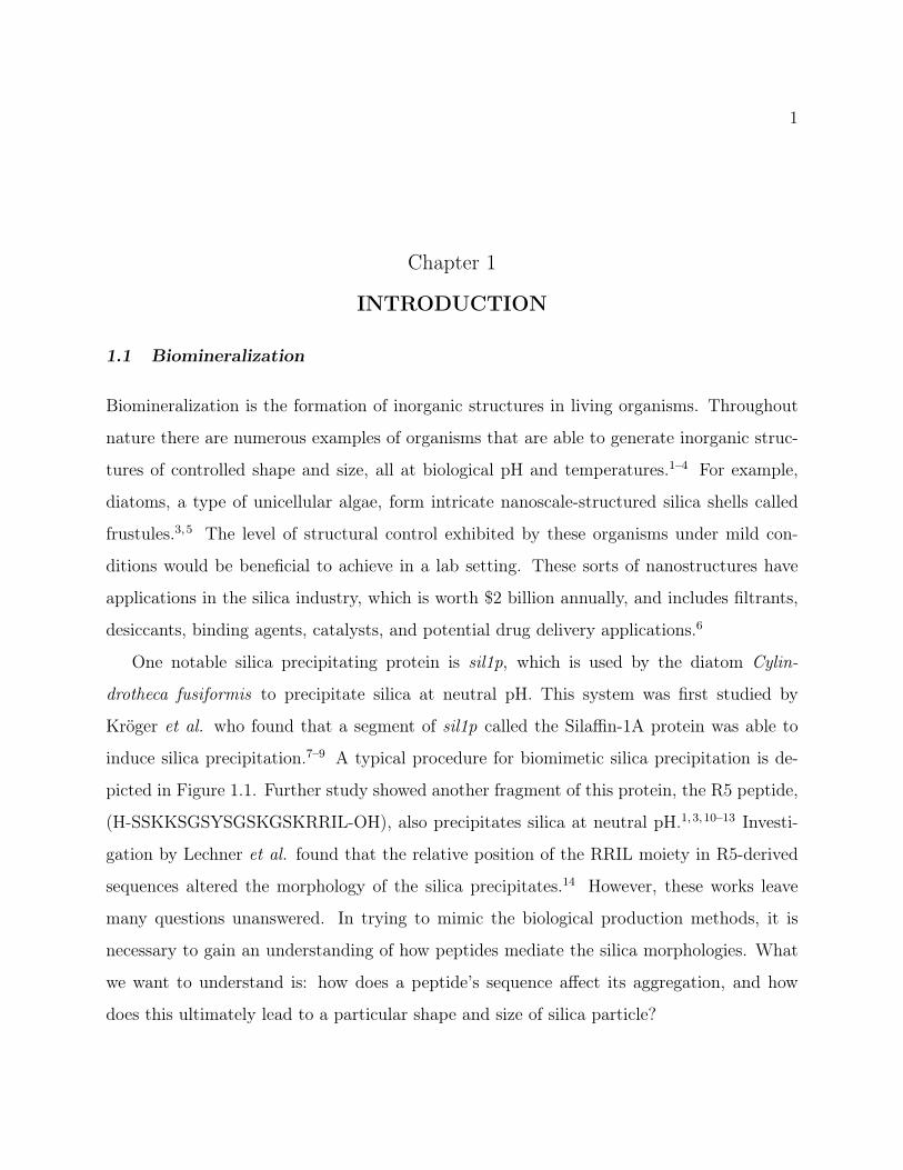
induce silica precipitation.7–9 A typical procedure for biomimetic silica precipitation is de-
picted in Figure 1.1. Further study showed another fragment of this protein, the R5 peptide,
(H-SSKKSGSYSGSKGSKRRIL-OH), also precipitates silica at neutral pH.1,3, 10–13 Investi-
gation by Lechner et al. found that the relative position of the RRIL moiety in R5-derived
sequences altered the morphology of the silica precipitates.14 However, these works leave
many questions unanswered. In trying to mimic the biological production methods, it is
necessary to gain an understanding of how peptides mediate the silica morphologies. What
we want to understand is: how does a peptide’s sequence affect its aggregation, and how
does this ultimately lead to a particular shape and size of silica particle?
2
1.2 Synthetic Amphiphilic Peptides
To get a better understanding of the mechanism of peptide mediated silica precipitation, it
is advantageous to start with a simple peptide of known secondary structure. Minimizing
the size of the peptide limits the number of potential influencing interactions (i.e., sequence
length, composition, secondary structure, charge and polarity of side chains) and permits
evaluation of how specific interactions change the system. The LK peptides are a series of
synthetic amphiphilic peptides, designed by DeGrado and Lear, that satisfy both of these
constraints.15,16 These peptides are composed of different arrangements of hydrophobic
leucine (L) and hydrophilic lysine (K), which give a controllable secondary structure at
polar/apolar interfaces.
The work presented here focuses on just one of these peptides, LKα14 so named because
it is a 14-residue LK peptide (Ac-LKKLLKLLKKLLKL-OH) that has a well characterized α-
helical structure. The hydrophilic lysine residues organize to interact with the polar material,
while the leucine residues arrange themselves on the opposing surface of the helical peptide
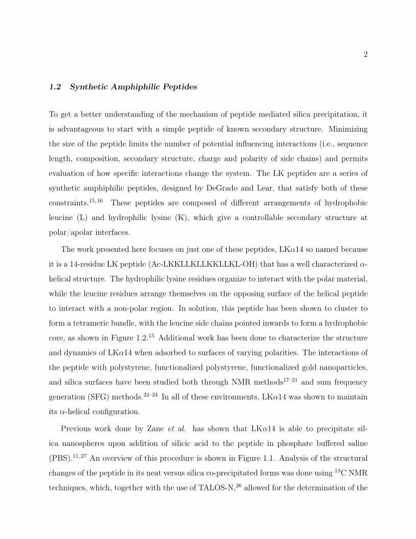
to interact with a non-polar region. In solution, this peptide has been shown to cluster to
form a tetrameric bundle, with the leucine side chains pointed inwards to form a hydrophobic
core, as shown in Figure 1.2.15 Additional work has been done to characterize the structure
and dynamics of LKα14 when adsorbed to surfaces of varying polarities. The interactions of
the peptide with polystyrene, functionalized polystyrene, functionalized gold nanoparticles,
and silica surfaces have been studied both through NMR methods17–21 and sum frequency
generation (SFG) methods.22–24 In all of these environments, LKα14 was shown to maintain
its α-helical configuration.
Previous work done by Zane et al. has shown that LKα14 is able to precipitate sil-
ica nanospheres upon addition of silicic acid to the peptide in phosphate buffered saline
(PBS).11,27 An overview of this procedure is shown in Figure 1.1. Analysis of the structural
changes of the peptide in its neat versus silica co-precipitated forms was done using 13C NMR
techniques, which, together with the use of TALOS-N,26 allowed for the determination of the
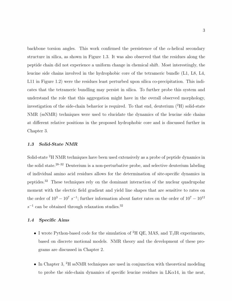
3
backbone torsion angles. This work confirmed the persistence of the α-helical secondary
structure in silica, as shown in Figure 1.3. It was also observed that the residues along the
peptide chain did not experience a uniform change in chemical shift. Most interestingly, the
leucine side chains involved in the hydrophobic core of the tetrameric bundle (L1, L8, L4,
L11 in Figure 1.2) were the residues least perturbed upon silica co-precipitation. This indi-
cates that the tetrameric bundling may persist in silica. To further probe this system and
understand the role that this aggregation might have in the overall observed morphology,
investigation of the side-chain behavior is required. To that end, deuterium (2H) solid-state
NMR (ssNMR) techniques were used to elucidate the dynamics of the leucine side chains
at different relative positions in the proposed hydrophobic core and is discussed further in
Chapter 3.
1.3 Solid-State NMR
Solid-state 2H NMR techniques have been used extensively as a probe of peptide dynamics in
the solid state.28–32 Deuterium is a non-perturbative probe, and selective deuterium labeling
of individual amino acid residues allows for the determination of site-specific dynamics in
peptides.32 These techniques rely on the dominant interaction of the nuclear quadrupolar
moment with the electric field gradient and yield line shapes that are sensitive to rates on
the order of 103 − 107 s−1; further information about faster rates on the order of 107 − 1012
s−1 can be obtained through relaxation studies.32
1.4 Specific Aims
• I wrote Python-based code for the simulation of 2H QE, MAS, and T1IR experiments,
based on discrete motional models. NMR theory and the development of these pro-
grams are discussed in Chapter 2.
• In Chapter 3, 2H ssNMR techniques are used in conjunction with theoretical modeling
to probe the side-chain dynamics of specific leucine residues in LKα14, in the neat,

4
buffered and silica-precipitated forms. The variations in the side-chain mobility in
different positions of the helix allows for predictions about the LKα14 aggregation
mode in spherical silica nanoparticles.
• Expanding on the basis developed for leucine, in Chapter 4, isoleucine dynamics are
quantified in the monomeric form, using 1D 2H and 2D 2H-13C NMR techniques.
Though a less symmetric–and therefore more complex–residue, isoleucine dynamics
are modeled using a similar approach.
• Chapter 5 presents work done in collaboration with Roy Black and Sarah Keller of
the Department of Chemistry at the University of Washington. 2H NMR techniques,
including static 2H NMR and 13C2H REDOR, were used to probe the interactions
of amino acids with fatty acid vesicles, as part of a study on the origin-of-life.

5
Figure 1.1: Overview of the procedure for silica precipitation mediated by LKα14. LKα14 is
a silica-precipitating peptide, PBS is phosphate buffered saline, Si(OH)4 is silicic acid, and
SiO2 is silica.
Figure 1.2: Helical wheel view of LKα14 arranged in a tetrameric bundle. Green Squares:
Leucine residues facing inwards to form a hydrophobic core; Purple Pentagons: hydrophilic
Lys residues exposed to interact with negatively charged SiO2; Sites highlighted in Orange
are the ones selected for further investigation in this work.
6
Figure 1.3: Chimera25 generated structures of LKα14 in the neat [top] and silica precipitated
[bottom] states, based on torsion angles obtained from TALOS-N.11,26
7
Chapter 2
NUCLEAR MAGNETIC RESONANCE THEORY
2.1 2H ssNMR Theory
The dominant interaction of the nuclear electric quadrupole moment with the electric field
gradient means that 2H ssNMR techniques are well suited for the characterization of dy-
namics.28–32 Solid state deuterium nuclear magnetic resonance techniques have been used
extensively as a non-perturbative, selective probe of peptide dynamics in the solid state in a
wide variety of conditions.28–32 Line shapes are sensitive to rates on the order of 103−107s−1
while faster motions with rates on the order of 107 − 1012 s−1 govern T1 relaxation.32
The full Hamiltonian operator describing the NMR spin system contains terms to quantify
interactions with both the external magnetic fields and the local interactions, and is given
by:28–31
H = Hz +Hrf︸ ︷︷ ︸external
+HCSA +HD +HJ +HQ︸ ︷︷ ︸internal
(2.1)
For deuterium, the magnitudes of the Zeeman (Hz) and quadrupolar (HQ) interactions are
76 MHz (for an 11.74 T magnet) and 170 kHz (for an sp3 hybridized C-2H), respectively.
These values dwarf the contributions from the chemical shift anisotropy (HCSA), dipolar
coupling (HD) and J-coupling (HJ). The effect of a radio-frequency pulse is described by
Hrf , this can be dropped from the Hamiltonian as well because one considers the state of
the system after the application of any pulses. Therefore, the Hamiltonian can be rewritten
simply as:
H ≈ Hz +HQ (2.2)
The first term represents the Zeeman effect, which is the result of the interaction of the
nuclear spin with the static magnetic field (B0); in practical terms, this is the result of

8
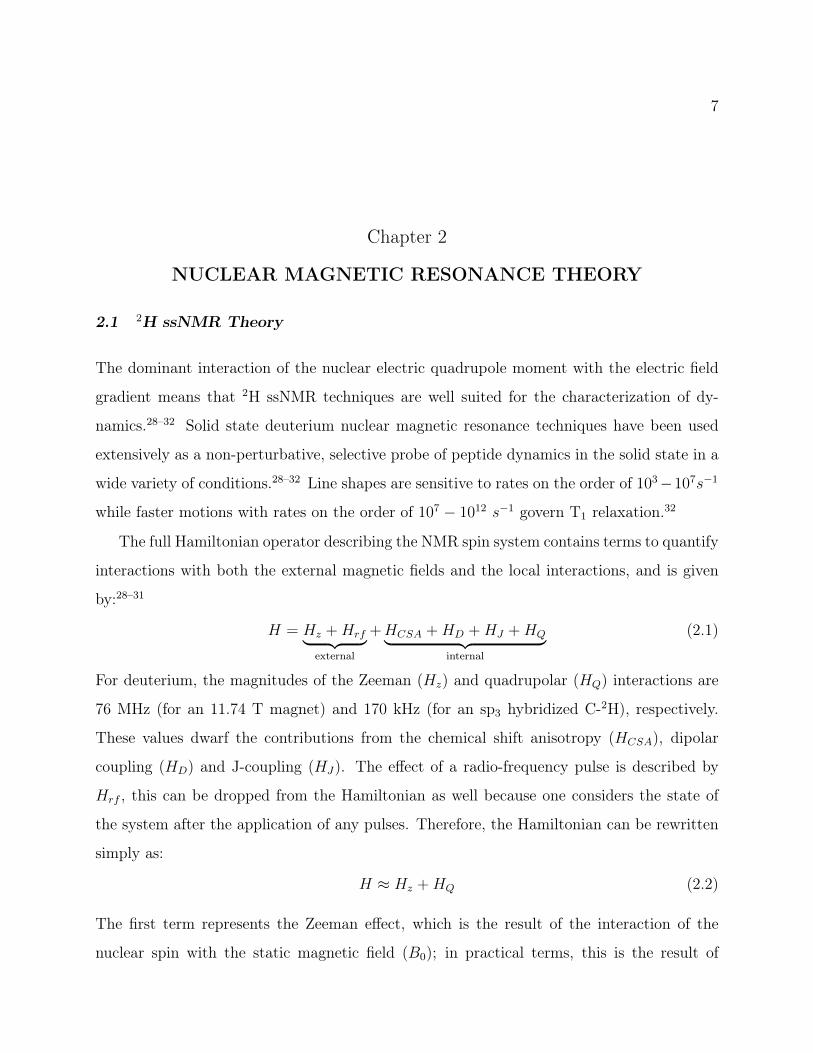
Figure 2.1: a) The splitting of the energy levels upon introduction into a static magnetic
field, followed by additional perturbation due to the quadrupolar interaction. (Drawing not-
to-scale). b) The static line shape, called the Pake doublet, where ωQ marks the position of
the "horns" corresponding to an EFG orientation of θ = π2.
simply placing a sample into the magnetic field. This interaction leads to the removal of the
energetic degeneracy of the spin states; shown in Figure 2.1a. For deuterium this leads to
three distinct spin states, corresponding to Iz = 0,±1, (where Iz is the component of the
spin angular momentum operator in the direction of the applied field, B0). The Zeeman
Hamiltonian, given in Equation 2.3, is dependent on the Larmor precession frequency, ω0.
This in turn depends on the strength of the field (B0) and the gyromagnetic ratio (γ). The
gyromagnetic ratio is a nucleus-dependent value, and is 6.536 MHz T−1 for 2H. Hence the
interaction has a magnitude of 76.77 MHz in an 11.74 T field. The energy of the splitting is
proportional to this frequency, as depicted in Figure 2.1.
Hz = −γIzB0 = −ω0Iz (2.3)
The quadrupolar Hamiltonian describes the interaction of the electric field gradient (EFG)
with the nuclear quadrupole moment:
HQ =
(eQ
2h
)I ·V · I (2.4)
where eQ is electric quadrupole moment of the nucleus, I is the nuclear spin vector, and V is
9
the second rank EFG tensor (in Cartesian coordinates). This tensor can be defined in terms
of its cartesian components: Vxx, Vyy, and Vzz. These values are more commonly reported
as eq, the principal component of the EFG and η, the asymmetry parameter:
eq = Vzz and η =Vxx − Vyy
Vzz(2.5)
The frequency of the perturbation by the quadrupolar interaction is dependent on the relative
orientations of the magnetic field and the deuterium EFG tensor, and is therefore a function
of both the magnitude and orientation of the quadrupole tensor relative to the magnetic
field, which is represented with the Euler angles, (0, θ, φ):
ωQ =3
4
(e2qQ
~
)︸ ︷︷ ︸
QCC
[3 cos2 θ − 1 + η sin2 θ cos 2φ] (2.6)
The simplest NMR line shape generated from this interaction is the axially symmetric
(η = 0) line shape of a "frozen" sample, shown in Figure 2.1b. This line shape is called a Pake
doublet, and represents the sum of the spectra resulting from the two possible Iz transitions,
1 → 0 and 0 → −1, shown separately in the bottom panel of Figure 2.1b. The frequencies
are derived from the expression for ωQ, and the intensities are weighted by sin θ, as a result
of the integration over all possible crystallite orientations in a disordered sample, referred to
as powder averaging. The interaction is therefore at a maximum when θ = π2, which gives
rise to the "horns" of the Pake doublet. The splitting of these horns is proportional to the
quadrupolar coupling constant (QCC or CQ), indicated in Equation 2.6. Note that there is
some variation in the literature of the definition of the QCC. Here we follow the convention
of QCC = e2qQh
, and this is the number input into the program. (The factors of 34and 2π
are explicitly applied within the code)
2.2 Overview of 2H ssNMR Experiments
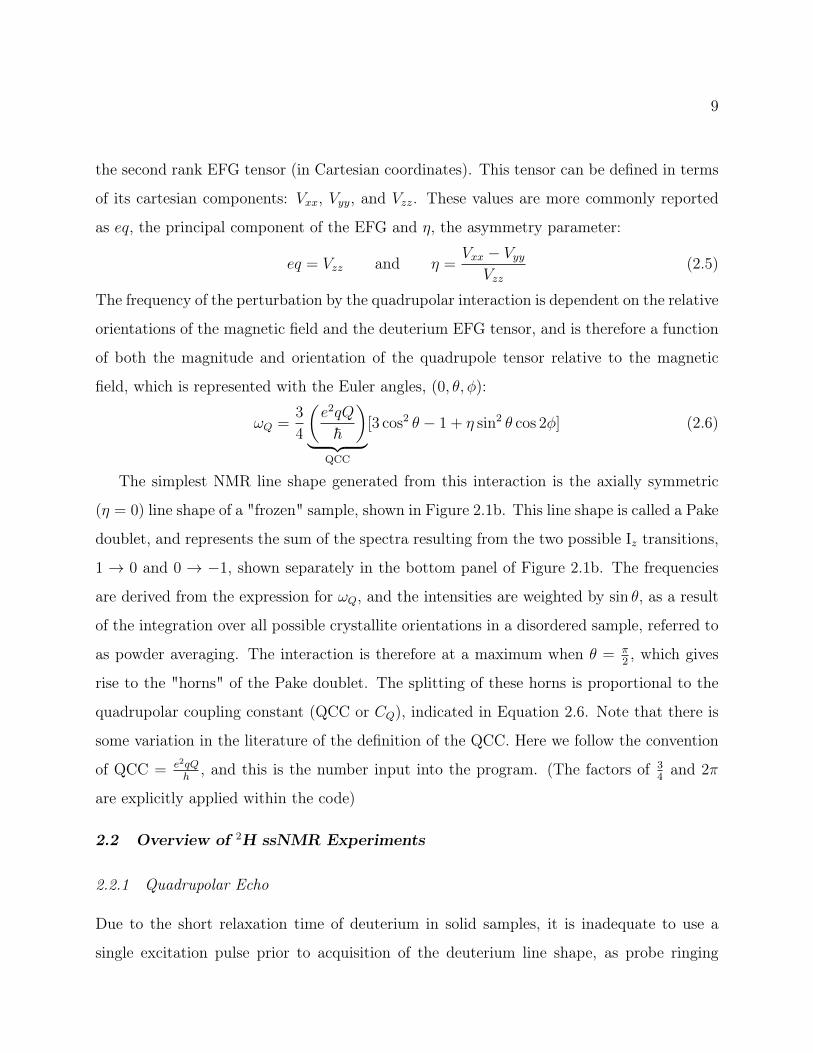
2.2.1 Quadrupolar Echo
Due to the short relaxation time of deuterium in solid samples, it is inadequate to use a
single excitation pulse prior to acquisition of the deuterium line shape, as probe ringing

10
and dead time would interfere with the signal. Instead, a quadrupolar echo pulse sequence,(π2
)x− τ1 −
(π2
)y− τ2 − acqu, is used, with phase cycling to suppress unwanted coherence
pathways.30,31 The first pulse is an excitation pulse, followed by a refocusing pulse at time
τ1. In principle, this should regenerate the original FID after a second delay of the same
length. In practice, τ2 is shorter to account for the effects of the finite pulse length and the
FID must be left-shifted prior to Fourier transformation so that the signal starts at the echo
maximum.
2.2.2 Magic Angle Spinning
Magic angle spinning is a technique for improving the signal-to-noise ratio in the deuterium
line shape experiments. By spinning the sample rotor at an angle of 54.74° relative to the
static magnetic field, the spectrum is split into a set of sharp, evenly spaced sidebands.33
This is because spinning at the so-called "magic angle" leads to a reduction of the first-
order quadrupolar line broadening, due to the angular dependence of this interaction: ∝
(3 cos2 θ − 1). This experiment has the added benefit of increasing the relaxation time, and
so does not require a pulse-echo sequence.
2.2.3 T1 Inversion Recovery
To probe the faster motions in the system, a inversion recovery quadrupolar echo sequence,
π− τR−(π2
)x− τ1−
(π2
)y− τ2− acqu, is used to determine the longitudinal relaxation time.
The time for the spin to relax after the inversion pulse depends on fluctuations in the local
magnetic field in the vicinity of the nucleus and therefore is dependent on the molecular
motions. By varying the length of the delay after the inversion pulse, this value can be
determined experimentally.
2.3 2H NMR Simulations
In starting to model my data, I was originally using EXPRESS, a publicly available MATLAB
program,34 to simulate the 2H NMR line shape resulting from exchange between discrete
11
τ1 τ2 acquπ2
π2
Figure 2.2: Quadrupolar Echo Pulse Program
acquπ2
Figure 2.3: Magic Angle Spinning Pulse Program
τR τ1 τ2 acquπ π
2π2
Figure 2.4: T1IR Pulse Program

12
conformations. This can be used in conjunction with additional MATLAB scripts to add
to its functionality. However, since the initial release of the program, MATLAB had been
updated and was slowly deprecating many features used in the GUI for the program. At the
same time, I was delving into the theory of the line shape simulations to better understand
how to approach my data fitting, and I ultimately decided to write my own code for the
simulations in Python. The formalism governing the simulation of dynamics-based line
shapes is well reported in the literature;29,31,35 so will be presented here only in brief. As
with EXPRESS, for a model with N discrete sites, the calculation of the spin system’s
response was done by integration of the Liouville equation.
But why reinvent the wheel?
In terms of the theory implemented, my Python methods do not differ heavily from EX-
PRESS for the simulation of the quadrupolar echo and T1IR data. However, it varies dra-
matically for the MAS simulations, where I implement the numerical integration method
published by Duer and Levitt (discussed below).36 Performance was also dramatically im-
proved allowing for significantly faster calculations (benchmarks below). In addition to being
a phenomenal learning exercise for me personally, there are several reasons Python is a prefer-
able platform for this code when compared to MATLAB. (Note: This list is based on my
own experiences and is corroborated by a plethora of others.37,38)
• Python is free. Unlike MATLAB, which requires a paid license and additional fees
if you require the functionality of additional packages.
• Python is open-source. Whereas MATLAB is proprietary and behaves as a black
box, Python packages have easily viewable (and editable) source code.
• Python is open. "There is a vigorous, healthy public debate on virtually all aspects
of Python, with input from any developer or user who wants to participate."37 This
level of interest and involvement also means there is active support for the user.
13
• Python is modular. Not only can you download preexisting modules, Python allows
you to define multiple functions in a separate file and import them to your main file.
To do that in MATLAB, each function would have to go in your main file, or in it’s
own individual file, which means similar helper functions cannot be neatly grouped
and the number of files needed is large.
• Python is more readable than MATLAB code. For example, Python indicates
blocks of code–for loops, if-then statements–by the indentation, making it easy to scan
through code and follow the logic. On the other hand, MATLAB blocks are finished
by an explicit "end" statement. This sort of closure means that the code is lengthier,
harder to debug and more daunting to parse through. Ease of comprehension when
looking at code – be it your own or a past student’s – is crucial for productivity.
• For the transferability of skills, Python is closer to the standard. Like C/C++, Java,
Perl, and most other programming languages other than MATLAB, Python conforms
to certain de facto standards, including zero-based indexing and the use of square
brackets rather than parentheses for indexing. This is an advantage for programmers
who must implement published signal processing algorithms, convert code from one
language to another, or work across many languages.
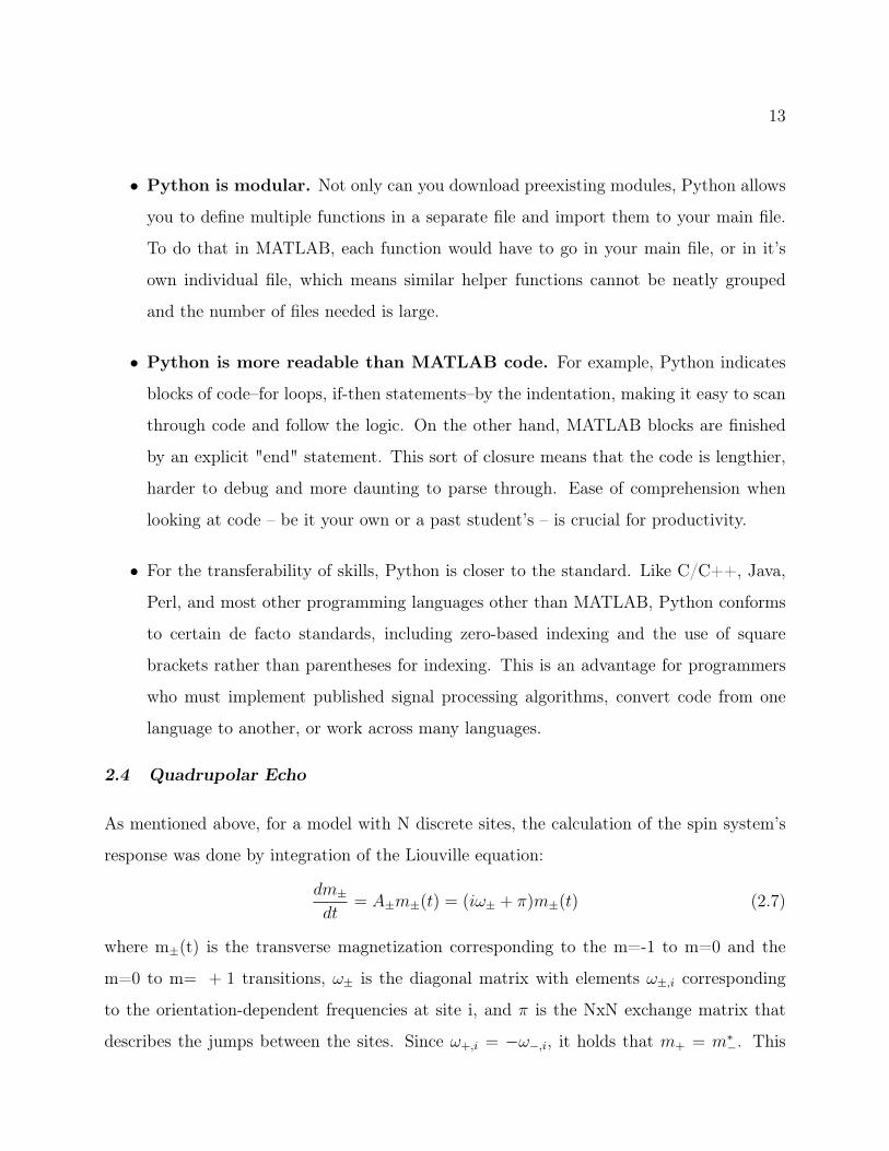
2.4 Quadrupolar Echo
As mentioned above, for a model with N discrete sites, the calculation of the spin system’s
response was done by integration of the Liouville equation:
dm±dt
= A±m±(t) = (iω± + π)m±(t) (2.7)
where m±(t) is the transverse magnetization corresponding to the m=-1 to m=0 and the
m=0 to m= + 1 transitions, ω± is the diagonal matrix with elements ω±,i corresponding
to the orientation-dependent frequencies at site i, and π is the NxN exchange matrix that
describes the jumps between the sites. Since ω+,i = −ω−,i, it holds that m+ = m∗−. This

14
means that the two transitions generate signals in the frequency domain that are mirror
images of each other, and therefore only one of these responses is calculated, in this case m+.
Equation 2.7 can be formally integrated to get:
m+(t) = eA+tm+(0) = L(t)m+(0) (2.8)
For the quadrupolar echo experiment, after the first pulse, during τ1, the response evolves
according to this equation, until the second π2pulse. This second pulse is a refocusing pulse
that interchanges m+ and m−, resulting in magnetization which is represented as:
m+(τ1) = eA∗τ1m+(0) (2.9)
The magnetization after the second delay, τ2, is then represented as:
m+(τ1, τ2) = eAτ2eA∗τ1 ·m(0) (2.10)
Finally, the expression for m+(t, τ1, τ2) representing the signal evolution after the τ2 delay,
is obtained by combining Equations 2.8 and 2.10:
m+(t, τ1, τ2) = eA(t+τ2)eA∗τ1 ·m(0) (2.11)
In practice, the matrix exponential is computationally expensive to compute. Note that,
in the past, it has been necessary to compute the matrix exponentials in Equation 2.11 by
diagonalizing A. However both MATLAB and Python’s scipy package include a function
that eliminate this step, and instead make use of the Padé approximation to permit the direct
input of matrix exponential. Additionally, to decrease the number of times this function is
called, instead of calculating the matrix exponential for each time point, t, an incremental
propagator is calculated and the signal response is calculated iteratively, as follows:36
m+(n∆t) = eA(∆t)m+((n− 1)∆t, τ1, τ2) (2.12)
with
m+(0, τ1, τ2) = eAτ2eA∗τ1m+(0) (2.13)
15
To further expedite the speed of calculation, the eAτ2 term is also dropped from the calcu-
lation, as it is computationally more efficient to generate these points with the incremental
propagator in Equation 2.12, and then left shift the calculated FID by τ2/∆t points prior to
Fourier transform. The signal at time t is the sum of all the contributions, that is:
s+(t, τ1, τ2) = 1 ·m+(t, τ1, τ2) = 1 · eA(t+τ2)eA∗τ1 ·m(0) (2.14)
2.4.1 Orientational Dependence
Powder averaging
The solid samples used for static deuterium NMR are, in most cases, powders with crystallites
of all possible orientations. The calculated signal in Equation 2.14 is dependent on the
orientation of the sample in the magnetic field, that is, the relative orientation of the crystal
frame (C) and the lab frame (L), is defined by an angle, ΩCL. The 2H NMR line shape is
obtained by integrating the Fourier transform of the time dependent signal, s(t), over all
possible sample orientations, ΩCL = (0, θCL, φCL):
I(ω) =
2π∫0
dφCL
π∫0
dθCL sin θCL Re
∞∫
−∞
dt s+(t)e−iωt
(2.15)
In practice, it is not possible to implement a continuous integral over s+(t), as in Equation
2.15; instead the signal is simulated as the sum over a set of crystal orientations and recorded
at discrete time points. Using the tiling method suggested by Vold et al. in the EXPRESS
documentation, ZCW (Zaremba-Conroy-Cheng) tiling is employed.34 See Appendix B.3 for
information of the generation of these angles. While executing the sum over these orientations
as a loop is less memory intensive, it is faster to construct higher dimensional matrices and
parallelize the sum using numpy’s einsum function (or more recently, the matmul function)
on stacks of matrices/vectors. See Appendix B.1.1 for implementation in the simulation
code.
16
Calculation of ωi: Motional frames
Motions are defined as jumps between discrete sites, where for a given site, i, ΩPC,i is the set of
Euler angles that transform the principal component axis system for the EFG tensor, P, into
a crystal-fixed axis system, C. (If additional motional frames are desired, intermediate frames
(I) are inserted between the principal frame and the crystal-fixed frame. For example, for a
model with two motions, ΩPI and ΩIC are defined. These intermediate frames are collapsed
into a single set of Euler angles prior to calculating the signal.) Euler angles here follow the
Rose or zyz convention, that is for an angle set ΩPC = (α, β, γ),
1. Rotate xyz in the principle axis frame counterclockwise around the z axis by α to give
x′y′z′.
2. Rotate the intermediate x′y′z′ counterclockwise around its y′ axis by β to give x′′y′′z′′.
3. Rotate x′′y′′z′′ counterclockwise around its z′′ axis by γ to give the final xyz in the
crystal frame.
Mathematically, the one frame equivalent sites are generated by the following matrix formal-
ization (see Appendix B.2.2 for implementation):
R(α, β, γ) = e−iαIze−iβIye−iγIz
=
cosα − sinα 0
sinα cosα 0
0 0 1
cos β 0 sin β
0 1 0
− sin β 0 cos β
cos γ − sin γ 0
sin γ cos γ 0
0 0 1
(2.16)
As mentioned above in equation 2.7, A± = ±iω + π and describes a model with N sites,
where ω is a diagonal NxN matrix of the orientation dependent frequencies, ωi:
ωi =3
4
e2qQ
~
2∑a=−2
(D
(2)0,a(ΩPC,i) +
η√6
(D
(2)2,a(ΩPC,i) +D
(2)−2,a(ΩPC,i)
))D
(2)a,0(ΩCL) (2.17)
where D(2)m′,m (α, β, γ) are terms of the rank-two Wigner rotation matrices, defined as:
D(2)m′,m (α, β, γ) = e−im
′αd(2)m′,m (β) e−imγ (2.18)

17
where d(2)m′,m (β) are the elements of Wigner’s small d-matrices, listed in Table 2.1.
Assuming that the C-H asymmetry parameter, η, is 0, Equation 2.17 simplifies to:
ωi =3
4
e2qQ
~
2∑a=−2
D(2)0,a(ΩPC,i)D
(2)a,0(ΩCL) (2.19)
The elimination of the η term is a limit on the versatility of this program, however the sim-
plification does mean fewer calculations, and therefore faster simulation times. Examples for
the definition of these frames are included in Appendix A.2, and the method for calculating
these terms is included in Appendix B.2.3.
2.4.2 Calculation of π: Site populations and exchange
The second part of the propagator, π, is a symmetric NxN matrix of the exchange rates
between the sites. It is constructed with off diagonal terms, πij, satisfying microscopic
reversibility, i.e. kijpj = kjipi, where kij is the rate of jumps from site j to site i and pi is the
population of site i. The diagonal terms, πii, corresponding to the rate of depletion of site
i. If it is not the case that all the sites are occupied equally, the matrix A is symmetrized
as A′ = P−1AP , where P is the diagonal matrix such that Pii = (pi)1/2. This can be
accomplished by manipulating just the π term of A, since the frequencies lie along the
diagonal and remain unchanged. Then the new jump matrix π′ is:
π′jk = π′kj = kjk (pk/pj)1/2 = kkj (pj/pk)
1/2 (2.20)
Note that for simplicity, the user is not asked to construct a full rate matrix where all kij
satisfy microscopic reversibility. Like EXPRESS, to minimize error, the user is asked for a
single rate value for each frame of motion, k, such that k = (kkj + kjk)/2. The jump matrix
is then calculated as:
π′jk = π′kj =2k(pjpk)
1/2
pj + pk(2.21)
Since P is invertible, the following equivalency holds eA′ = eP−1AP = P−1eAP . From this it
follows that eA = P · P−1eAP · P−1 = PeA′P−1. Substituting this into Equation 2.14, where

18
@@
@@
@@ @
m′ =
m=
21
0-1
-2
2( 1
+co
sβ
2
) 2−
sinβ
2(1
+co
sβ
)
√ 3 8si
n2β
−1 2
sinβ
(1−
cosβ
)
( 1−
cosβ
2
) 2
1si
nβ
2(1
+co
sβ
)1 2
( 2co
s2β
+co
sβ−
1)−√ 3 8
sin
2β1 2
( −2co
s2β
+co
sβ
+1)−
sinβ
2(1−
cosβ
)
0√ 3 8
sin
2β
√ 3 8si
n2β
1 2
( 3co
s2β−
1)−√ 3 8
sin
2β
√ 3 8si
n2β
-1si
nβ
2(1−
cosβ
)1 2
( −2co
s2β
+co
sβ
+1)
√ 3 8si
n2β
1 2
( 2co
s2β
+co
sβ−
1)−
sinβ
2(1
+co
sβ
)
-2( 1−
cosβ
2
) 2si
nβ
2(1−
cosβ
)
√ 3 8si
n2β
sinβ
2(1
+co
sβ
)
( 1+
cosβ
2
) 2Ta
ble2.1:
Elements
ofRan
k-2W
ignersm
alld
-matrices
19
m+(0) is the site populations, pi gives the equation for the signal:
s+(t) = m+(0)1/2 · eA′(t+τ2)eA
′∗τ1 ·m+(0)1/2 (2.22)
2.5 MAS Simulations
For MAS spectra, the solution to 2.7 is not so simple as that for the static spectra, given in
Equation 2.12. The manual rotation of the sample in the rotor means that it is not simply
the case that L(t) = expiω + π because the orientation is now changing with time and so
L(t) now depends on ω(t).39–42
2.5.1 Numerical Integration
Following in the footsteps of Duer and Levitt,36 the method employed here is to numerically
integrate, and solve for L(t) over the course of a single rotor period, that is, to generate it
on the range 0 < t < τr. The rotor period, τr is divided into n steps, that are sufficiently
small so it can be assumed that the orientation is approximately constant over the interval
and such that ∆t = τrn
= 1νrn
, where νr is the rotation frequency. Then, the center of each
∆t step is defined as tm = (m − 12)∆t for m = 0, 1, 2, ...n. Then L during the rotor period
can be calculated as:L(m∆t) = e(iω(tm)+π)∆t · L((m− 1)∆t)
L(0) = 1(2.23)
Generally, n = 64 is close to a fair approximation and can be used for preliminary testing
of a given model. Full convergence can require smaller steps, with n=128 or 256, consistent
with the values reported by Kun Li.43 Note that while powers of two are not technically
required for this method, the further propagation of the signal is coded to be most efficient
when the number of fractions and the number of FID points calculated are both powers of
two; see Appendix B.1.2 for more information. Once this is calculated for the first rotor
period, the rest of the L(t) values are calculated as:
L(t+Mτr) = L(τr)ML(t) (2.24)

20
This straightforward method is not the only one used; see below for discussion of the method
used in EXPRESS.
Calculation of ωi(t) and tiling
While the static spectra only require two-angle tiling for the integration, the transforma-
tion from the MAS frame to the laboratory frame requires a full three-angle tiling set be
used. This is more easily seen looking at the calculation of the orientation dependent site
frequencies:
ωi(t) =3
4
e2qQ
~
2∑a,b=−2
D(2)0,a(ΩPC,i)D
(2)a,b(ΩCL)D
(2)b,0 (ΩLM(t)) (2.25)
where ΩLM(t) = ΩLM(m∆t) = (2πnm∆t, θmagic, 0). The tiles used here are the optimized
ZCW3 sets, and are not calculated like the two-angle sets used for the quadrupolar echo
experiments.44–46 They are stored for a few fixed values and imported as needed.47 See
Appendix B.3 for more information.
2.5.2 Floquet Theory Comparison
Another method commonly used for simulating these line shapes exploits the periodicity of
these orientations to construct a new time-independent operator, using a Floquet expan-
sion.34,36 This can then be used as in Equation 2.12. In EXPRESS, the user is asked the
"number of sideband pairs" they want to simulate in their spectrum, a somewhat mislead-
ing label, as the documentation recommends that the user select a number 2-3 times the
number desired. Looking into the algorithm used to construct this operator, one finds that
the simulation generates a square matrix with a length of (2× nside + 1)× nsites, compared
to the propagator for the static simulations which is a square matrix with dimensions of
nsites × nsites. In the documentation for EXPRESS, it is noted that the majority of their
computational time is spent, not on the matrix exponential, but on the recursive FID prop-
agation by matrix multiplication, and they use this to, in part, justify their method. I would
21
like to note that the numerical integration method presented above uses smaller matrices
and therefore dramatically decreases the amount of time required for the calculations.
2.6 T1IR Simulations
The addition of the π pulse at a variable delay, τr, before the quadrupolar echo sequence
allows for the determination of the spin lattice relaxation rate, T1. For a given crystal
orientation, the signal can be calculated as in Equation 2.22, with just the addition of a
constant factor reflecting the extent of relaxation at time τr. Most simply this is given as:
m(τr) = m(0) ·(1− 2e−τr/T1
)(2.26)
The relaxation time, T1, depends on the strength of the magnetic field, ω0 and the crystal
orientation. It can be calculated from the spectral densities, Jm, as follows:28,34,35
1
T1
=3
16
(e2qQ
~
)(J1(ω0,ΩCL) + 4J2(ω0,ΩCL)) (2.27)
The form of the spectral densities has been derived previously in the literature (most useful
to this author was the presentation by Wittebort, et al.35). Note that the version here differs
in the ordering of the Wigner rotations, for example, the rotation ΩPC is used in place
of ΩCP , as this accounts for the flipped order of the subscripts of the Wigner-D rotation
matrices. Additionally, the sum is given in terms of the full Wigner-D rotation matrix,
whereas Wittebort simplifies it include only the Wigner small-d elements and a cosine term.
Jm(ω,ΩCL) = −22∑
a,a′=−2
D(2)∗am (ΩCL)D
(2)a′m(ΩCL)
×N∑
n,l,j=1
X(0)l X
(n)l X
(0)j X
(n)j D
(2)∗0a (ΩPC,l)D
(2)0a′(ΩPC,j)
λnλ2n +m2ω2
0
(2.28)
The X(n) and λn terms refer to the corresponding eigenvectors and eigenvalues of the jump
matrix, π, calculated as in Equation 2.21. Note that X(0) is taken to be the initial magneti-
zation vector with terms equal to p1/2i .
22
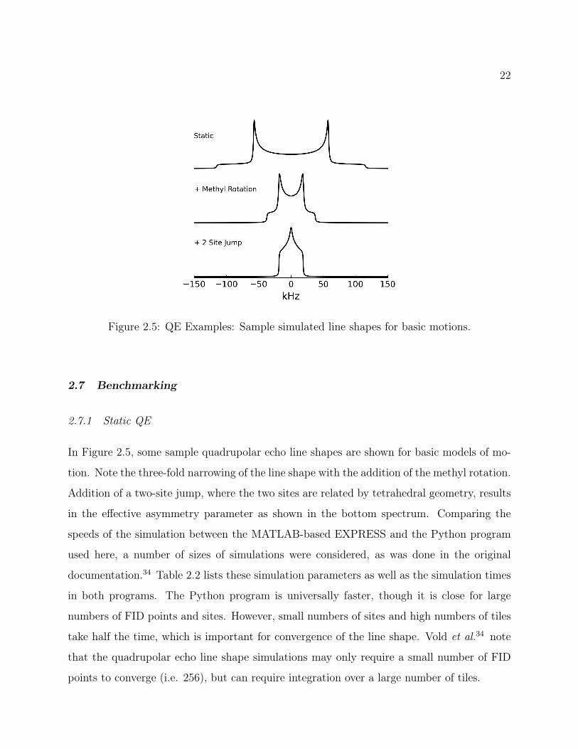
Figure 2.5: QE Examples: Sample simulated line shapes for basic motions.
2.7 Benchmarking
2.7.1 Static QE
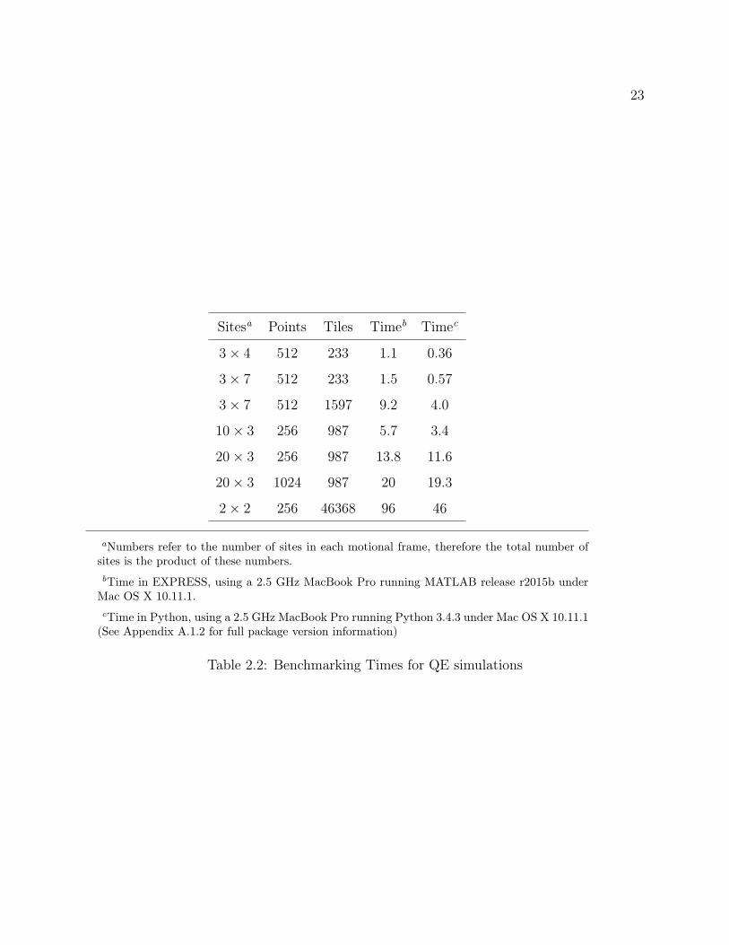
In Figure 2.5, some sample quadrupolar echo line shapes are shown for basic models of mo-
tion. Note the three-fold narrowing of the line shape with the addition of the methyl rotation.
Addition of a two-site jump, where the two sites are related by tetrahedral geometry, results
in the effective asymmetry parameter as shown in the bottom spectrum. Comparing the
speeds of the simulation between the MATLAB-based EXPRESS and the Python program
used here, a number of sizes of simulations were considered, as was done in the original
documentation.34 Table 2.2 lists these simulation parameters as well as the simulation times
in both programs. The Python program is universally faster, though it is close for large
numbers of FID points and sites. However, small numbers of sites and high numbers of tiles
take half the time, which is important for convergence of the line shape. Vold et al.34 note
that the quadrupolar echo line shape simulations may only require a small number of FID
points to converge (i.e. 256), but can require integration over a large number of tiles.
23
Sitesa Points Tiles Timeb Timec
3× 4 512 233 1.1 0.36
3× 7 512 233 1.5 0.57
3× 7 512 1597 9.2 4.0
10× 3 256 987 5.7 3.4
20× 3 256 987 13.8 11.6
20× 3 1024 987 20 19.3
2× 2 256 46368 96 46
aNumbers refer to the number of sites in each motional frame, therefore the total number ofsites is the product of these numbers.bTime in EXPRESS, using a 2.5 GHz MacBook Pro running MATLAB release r2015b under
Mac OS X 10.11.1.cTime in Python, using a 2.5 GHz MacBook Pro running Python 3.4.3 under Mac OS X 10.11.1
(See Appendix A.1.2 for full package version information)
Table 2.2: Benchmarking Times for QE simulations
24
2.7.2 MAS
As noted above, the Floquet method requires a propagator matrix of size (2nside + 1)nsites×
(2nside+1)nsites, while the numerical integration method requires a set of nrotfrac propagators
with size nsites × nsites. Take as an example a 6-site model, with a moderate spinning speed
that results in 10 side band pairs. The Floquet method would require 2-3 times that number
of sideband pairs to simulate it fully: say 25 sideband pairs, then the matrix has size:
((2nside + 1)nsites)2 = ((2(25) + 1)(6))2 = 306 × 306. Assuming the numerical integration
method converges with nrotfrac = 256, then the method requires nrotfrac×n2site = 256×(6×6).
Note that while this does mean that the numerical integration method requires 256 times as
many matrix exponentials to be performed, the size of those matrices is dramatically smaller.
Additionally, after the calculation for the first rotor period, the propagation of the signal
using the dot product requires only the set of 6× 6 matrices generated, whereas the Floquet
method requires multiplication by a matrix over 50 times as large.
2.7.3 T1IR
As demonstrated in Table 2.3, the Python-based program runs much faster than the MAT-
LAB version. Most notably, the Python version makes better use of array broadcasting
techniques and eliminates the extensive use of for-loops in the calculation of the relaxation
time. The for-loop method is more immediately understandable to a reader, and corresponds
more clearly to the summation notation used by Wittebort et al., however it is far less com-
putationally efficient. To show that the method does not alter the accuracy of the algorithm,
Figure 2.6 was generated using the sample parameters as presented by Vold et al., and is
presented for comparison with their results, see reference.34
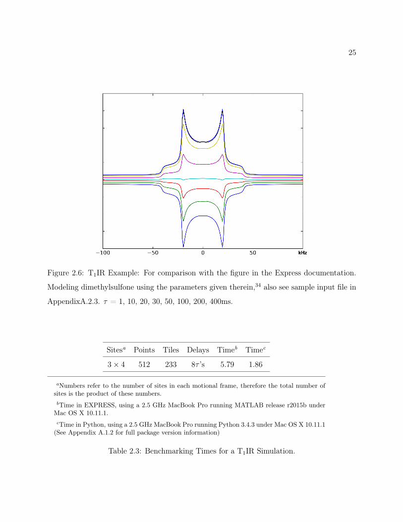
25
Figure 2.6: T1IR Example: For comparison with the figure in the Express documentation.
Modeling dimethylsulfone using the parameters given therein,34 also see sample input file in
AppendixA.2.3. τ = 1, 10, 20, 30, 50, 100, 200, 400ms.
Sitesa Points Tiles Delays Timeb Timec
3× 4 512 233 8τ ’s 5.79 1.86
aNumbers refer to the number of sites in each motional frame, therefore the total number ofsites is the product of these numbers.bTime in EXPRESS, using a 2.5 GHz MacBook Pro running MATLAB release r2015b under
Mac OS X 10.11.1.cTime in Python, using a 2.5 GHz MacBook Pro running Python 3.4.3 under Mac OS X 10.11.1
(See Appendix A.1.2 for full package version information)
Table 2.3: Benchmarking Times for a T1IR Simulation.
26
Chapter 3
BIOSILICIFICATION AND THE LKα14 PEPTIDE: MODELINGLEUCINE SIDE CHAIN DYNAMICS
As discussed in Chapter 2, 2H NMR can be used to determine information about dynam-
ics. Here this method is applied to evaluate the packing of LKα14 in silica, as well as in the
neat and buffered states for comparison. The peptide is thought to form a tetrameric bundle
(see Figure 1.2).
3.1 Qualitative Analysis of Leucine Dynamics
Leucine methyl group dynamics are very sensitive to the their environment. In a protein
hydrophobic core, motion is limited because the non-polar side chains are tightly packed
and more shielded from changes in the outside environment. Closer to the polar interface,
motion is increased because the steric hindrance is decreased. Smith et al. has used this
type of analysis to determine relative mobility of leucine residues along a peptide to probe
the relative packing orientations of helical peptides.48–50 Similarly, Long et al. applied this
analysis to determine the orientation of KL4, a lung surfactant peptide, in a phospholipid
bilayer.51
In the absence of motion, the spectrum will be the axially symmetric line shape of a
"frozen" sample, called the Pake doublet, shown in Figure 2.5a. 2H line shapes can be inter-
preted qualitatively in terms of their deviation from this Pake doublet, which is indicative
of molecular motions with a correlation time of 10−3 − 10−7 seconds. Rapid, axially sym-
metric motions, such as methyl group rotation, result in the narrowing of the spectrum, and
therefore decreased splitting between the horns and can be treated as effective decrease in
the QCC for modeling purposes, as shown in Figure 2.5b. Asymmetric motions, such as

27
rotameric exchange or diffusion of the methyl group along an arc, will result in an increased
central intensity and a corresponding decrease of the intensity of the horns, as shown in
Figure 2.5c.
3.2 Quantitative Motional Models for 2H NMR Simulations
The most important part, and sometimes the most difficult part, of fitting the spectral data
is choosing a physical model to parametrize. As discussed in Chapter 2, these models are
based on jump motions between defined sites. Complexity is added to these phenomeno-
logical models by adding additional frames of motion. This system of model development
complicates comparing systems, but it gives a model with a physical meaning that is more
intuitively comprehended. The lack of an analogous conceptualization is why a "model-free"
method such as the microscopic-order-macroscopic-disorder (MOMD) approach developed
by Meirovitch et al. are avoided in this work.52,53
3.2.1 Methyl Rotation
As mentioned in the qualitative analysis section, the rapid rotation of the methyl CD3 around
the Cγ-Cδ bond results in an overall narrowing of the line shape. For the purposes of QE and
MAS simulations, this motion means the methyl group deuterons can be approximated as a
single effective axially symmetric quadrupolar tensor along the Cγ-Cδ bond, with a decreased
QCC, which decreases the number of sites needed to model the spectra (and therefore the
computational time needed). For T1IR simulations, this simplification is not valid since T1
depends on faster rates, and the correlation time of these rapid motions must explicitly be
incorporated. This can be explicitly modeled as a three site jump around a C3v axis defined
by the Cγ-Cδ bond.
3.2.2 Rotameric Jumps
The leucine side chain is able to take on 9 different rotameric conformations, which are
the result of three possible torsion angles around each the Cα−Cβ (χ1) and Cβ−Cγ (χ2)
28
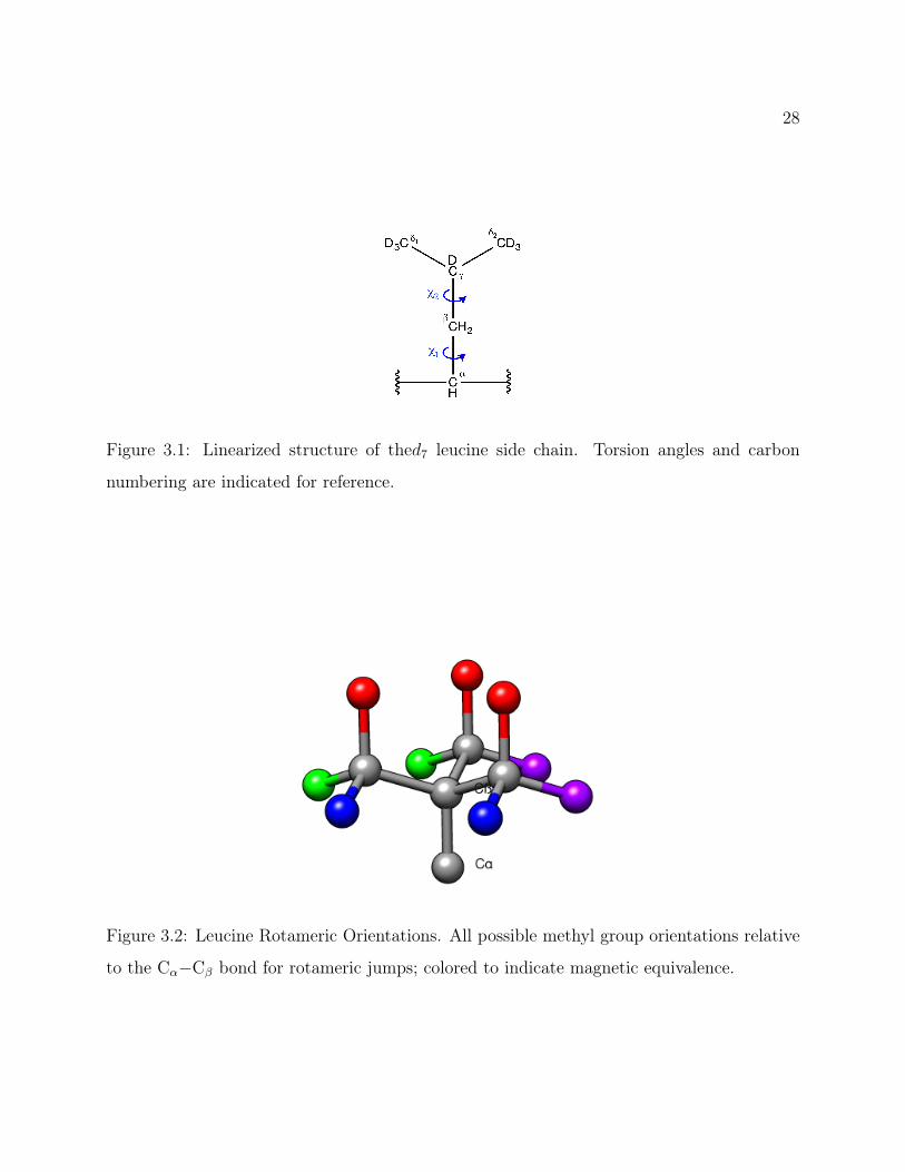
Figure 3.1: Linearized structure of thed7 leucine side chain. Torsion angles and carbon
numbering are indicated for reference.
Figure 3.2: Leucine Rotameric Orientations. All possible methyl group orientations relative
to the Cα−Cβ bond for rotameric jumps; colored to indicate magnetic equivalence.
29
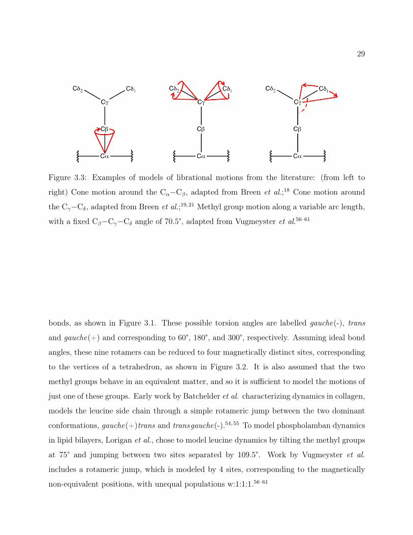
Figure 3.3: Examples of models of librational motions from the literature: (from left to
right) Cone motion around the Cα−Cβ, adapted from Breen et al.;18 Cone motion around
the Cγ−Cδ, adapted from Breen et al.;19,21 Methyl group motion along a variable arc length,
with a fixed Cβ−Cγ−Cδ angle of 70.5°, adapted from Vugmeyster et al.56–61
bonds, as shown in Figure 3.1. These possible torsion angles are labelled gauche(-), trans
and gauche(+) and corresponding to 60°, 180°, and 300°, respectively. Assuming ideal bond
angles, these nine rotamers can be reduced to four magnetically distinct sites, corresponding
to the vertices of a tetrahedron, as shown in Figure 3.2. It is also assumed that the two
methyl groups behave in an equivalent matter, and so it is sufficient to model the motions of
just one of these groups. Early work by Batchelder et al. characterizing dynamics in collagen,
models the leucine side chain through a simple rotameric jump between the two dominant
conformations, gauche(+)trans and transgauche(-).54,55 To model phospholamban dynamics
in lipid bilayers, Lorigan et al., chose to model leucine dynamics by tilting the methyl groups
at 75° and jumping between two sites separated by 109.5°. Work by Vugmeyster et al.
includes a rotameric jump, which is modeled by 4 sites, corresponding to the magnetically
non-equivalent positions, with unequal populations w:1:1:1.56–61

30
3.2.3 Librational Modes
Other models include not only the rotameric jumps, but also an additional perturbation due
to bond librations or backbone movement.62–65 For example, in work by Vugmeyster et al.
in addition to the rotameric jump the Cγ−Cδ bond is assumed to move along a variable-
length arc, shown in the right panel of Figure 3.3.56–61 Previous work characterizing LKα14
dynamics, by Breen et al., employed a two-site rotameric jump with additional librational
motion modeled as nearest neighbor jumps of a bond along a cone–around either the Cα−Cβ18
or Cγ−Cδ bond,19,21 as depicted in Figure 3.3.
3.3 Automation of Fitting
Defining the motional model with multiple sites and jump rates leads to a daunting number
of parameters to optimize. There are several approaches that can be taken. In studying
the chicken villin headpiece, Vugmeyster et al. generated libraries of spectra with varied
parameters, an approach made possible by the simplification of the problem to just 2-4
adjustable parameters. The line shapes were fit checking the quality of the fit for every
spectrum in the library.
With an increased number of variables, this is not a viable option, since the number of
possible parameter sets scales exponentially. Instead it is desirable to introduce an automated
search algorithm into the fitting program for global optimization of the paramters. Aliev and
Harris66 implemented simulated annealing to fit the QE spectra of thiourea-d4. A similar
approach has been used by Li et al. to fit 2H MAS line shapes and model the dynamics of
the phenylalanine side chain.67 There a simulated annealing algorithm was implemented to
minimize the difference in the intensities of the spinning sidebands in the spectra. I tried
using the simple downhill search, simulated annealing and threshold acceptance algorithms.
I prefer the threshold acceptance algorithm, but have included an overview of each of these
methods.

31
3.3.1 Simple Algorithm
The most straightforward random search method is to simply take random steps and accept
these steps if they improve the fit. The user defines a set of starting parameters, a step
size, and a goodness of fit metric. Based on the step size, a random new set of parameters
is generated. If this set of new parameters results in a spectrum that is a "better fit," this
parameter set is saved as the new best fit, otherwise the best fit is unchanged. This process
continues iteratively until an end condition is reached, generally either a total number of
steps taken, or a number of steps without improvement, which implies that the state is
optimized. This method invariably leads to a local minimum, but not necessarily a global
minimum.
3.3.2 Simulated Annealing
To overcome situations where the step size is too small to escape a local minimum, a simulated
annealing method was employed by Aliev and Harris.66 This method is similar to the simple
method described above, however it does not reject all steps that do not improve the fit. If a
parameter set is found to be the best fit seen, it is stored as the best fit. However, in addition
to accepting steps that improve the fit, the algorithm uses to Metropolis-Hastings method
and explores the parameter space by accepting steps that do not make the fit significantly
worse with some small probability e∆−E/T , where ∆E is the change in the energy or goodness-
of-fit parameter compared to the previous parameter set evaluated and T is a temperature
parameter.68,69 The temperature parameter, T, is set by the user and is decreased over
the course of the optimization according to a defined "cooling schedule", hence the term
"annealing". This means that the algorithm is more likely to accept steps that do not
improve the fit early in the optimization to better explore the parameter space, and less so
as the simulation is closer to converging.
32
3.3.3 Threshold Acceptance
The algorithm employed in this work is the threshold accepting algorithm.70,71 This method
is very similar to the simulated annealing method, but instead of only accepting worse fits
with a small probability, every fit that is only a little bit worse (under a certain threshold) is
accepted. The elimination of the random acceptance criterion guarantees a more thorough
traversal of the parameter space, and has been found to be a superior method. Analogous to
the "cooling schedule" employed in the simulated annealing method, the threshold value is
decreased if the quality of the fit has not been improved after some number of iterations. It is
also possible to decrease the step size to allow for a more localized search as the optimization
nears convergence.
3.3.4 Setting up an Optimization
Goodness-of-Fit
The most common goodness of fit method is a simple residual:
R2 =1
N
N∑i=1
(Iexpi − Isimi
)2 (3.1)
While often used, there are complications. Special concerns with automating the fitting
of these spectra include the non-discrete nature of these spectra. For the fitting of the
MAS spectra discussed previously the spectra were treated as a set of discrete intensities
corresponding to each sideband height. This simplified the fitting function by removing the
complications presented by the hard-to-fit sideband widths.
With static line shapes, one is faced with the complicating factors of the mild asymmetry
present in the experimental data and the complication of residual water contributing an
isotropic peak, which should not be fit by the model, but leads to a significant distortion
when using a fitting metric based solely on spectral intensity. Vugmeyster et al. used
alternative indicators of goodness-of-fit: possibilities include horn splitting, width of the line
shape at half height, and width of the spectrum at the shoulders.56,57
33
In work presented here the goodness of fit metric used was a modified R2. It was modified
to include a sub-optimization (performed using a built in scipy routine) to account for several
factors, referred to here as x. Firstly, offsets in the height or scaling were accounted for
by optimizing a vertical offset, x[1], and scaling factor, x[0], rather than attempting to
perfectly optimize the baseline and normalize based on peak height alone. Second, the spectra
include contributions from the Hγ in addition to the methyl groups. This contribution is not
necessarily stoichiometric due to attenuation because of the longer relaxation time. Rather
than including this as a parameter in the search, the contribution was determined after the
fact, by scaling the contribution to the spectrum of Hγ by a factor, x[2]. Finally, the water
peak was modeled as a Lorentzian line shape (y = 11+x2
) with variable width (x[4] = 1-4 Hz)
and variable contribution scaled by x[3], to account for the central distortions. Overall this
lead to a final spectrum as follows:
S = x[0] (Smethyl + x[2] ∗ Sγ) + x[1] + x[3] ∗ Swater (3.2)
Threshold, Step Size, and Starting Point
These parameters require some testing to optimize. The threshold needs to be large enough
that the optimization adequately explores the parameter space, but large enough to prevent
all steps from being accepted. One back-up measure to prevent a search from just endlessly
climbing up hill is to set a maximum energy value that the state can have. However, it is
usually better to adjust the threshold and step size relative to each other.
Step size should similarly be big enough to adequately explore the space, without being
so large that it is too random. An even bigger concern is unbalanced step size, that is, one
parameter exploring the space insufficiently compared to the rest of the set. This leads to
the local minima one wants to avoid. The easiest example is allowing the QCC to change
a lot compared to the jump rate(s) and population(s). The search algorithm can get stuck
in a local minimum where the QCC was adjusted to fit the spectral width (especially since
the steep slope has a big effect on the R2) but doesn’t fit the overall line shape well, when a

34
larger QCC and increased motion may be better.
Other parameters than can be changed are the number of steps to take without improve-
ment before decreasing the threshold (and step size) and how much to decrease them by.
More steps and slower decrease of step size and threshold, guarantees a better exploration
of the parameter space, but takes longer. In cases with a large number of parameters it
is beneficial to try a variety of settings for all of these parameters discussed. Lastly, it is
important to start with a model that is somewhat close to fitting the data. While this is not
necessary, it does help significantly.
Multiple Spectral Types
Finally, the absolute fit of any one type of data is not the best indicator of the accuracy of a
model. The use of different, overlapping methods constrains the model. The best fit of the
QE data will not necessarily be the best fit of the MAS and T1IR data because each method
is sensitive to slightly different rates. This is demonstrated later.
3.4 Methods
3.4.1 LK Synthesis
Labelled leucine was singly incorporated into peptide samples, i.e., L8 indicates l-leucine-
(isopropyl-d7) was incorporated at position 8. One of the peptides, L11, was synthesized by
a previous group member, Dr. Nicholas Breen, on a Rainin PS3 instrument, as previously
reported.18 Additional L11 sample was required and synthesized using a CEM Liberty Blue
Automated Microwave Peptide Synthesizer using standard FMOC chemistry, followed by
acetylation of the N terminus. After cleavage, the purity was determined by mass spectrom-
etry. No further purification was required.
In addition to peptides that were synthesized in-house, two peptides were purchased from
Anaspec (Fremont, CA) with d7-2H labels at the L5 and L8 sites, respectively.
35
3.4.2 Silica Precipitation
As previously reported,11 silica samples for NMR studies were prepared by first dissolving
peptide (∼25mg) in 1 x PBS (5 mL) to give a 3 mM solution. While the peptide dissolved, 1M
Si(OH)4 (silicic acid) was prepared by dissolving 0.15 mL TMOS (tetramethyl orthosilicate)
in 0.85 mL 1 mM HCl. 1M Si(OH)4 (0.5 mL) was added to the buffered peptide solution; the
mixture was vortexed and allowed to incubate for five minutes at room temperature. After
silica precipitation, the sample was centrifuged, washed (3 x 5 mL DI water), and dried en
vacuo.
3.4.3 NMR Sample Preparation
The neat peptide was lyophilized from a solution of 3 mM LKα14 in deionized water. For
hydrated samples, this sample was then hydrated to ∼40% by mass, to reinstate native
dynamics.59,72 This was achieved by diffusion of deuterium-depleted water into the sample
rotor. The PBS-peptide samples were prepared analogously to the neat samples, but from
PBS buffer instead of water. Silica-peptide co-precipitate was prepared as described above,
and analyzed without further treatment.
3.5 NMR Experimental Methods
3.5.1 2H Quadrupolar Echo Lineshapes
All static quadrupolar echo experiments were performed at 11.74T field (76.77 MHz deu-
terium Larmor frequency) using a home-built, single-channel, static deuterium probe with
a Bruker Avance III spectrometer and a π2pulse time of 2.9 µs. Quadrupolar echo experi-
ments used eight-step phase cycling, with an echo delay of 40 µs, and a recycle delay of 0.4s.
Line shapes were processed by left-shifting to the echo maximum prior to Fourier transform,
followed by 1 kHz line broadening and phase correction.
36
3.5.2 2H T1 Inversion Recovery
T1Z measurements were also acquired at 11.74T, using an inversion recovery pulse sequence
with quadrupolar echo detection. Six variable delays were used [500ms, 100ms, 50ms, 25ms,
10ms, 1ms], and 160k scans were acquired for each time point, and processing was performed
as for the line shapes.
3.5.3 2H Magic Angle Spinning
MAS line shapes were acquired with the same magnetic field, but with a Bruker TriGamma
probe. These experiments employed a single 2H π2pulse width of 3.4 µs and were performed
with spinning speeds of 4 kHz. 60k-200k scans were collected, depending on the spectrum,
with a 1s relaxation delay between scans. After left-shifting to the peak of the first echo,
FIDs were Fourier transformed and phase-corrected without further processing.
3.6 Results
3.6.1 Qualitative 2H Line Shape Analysis
As shown in Figure 3.4, line shapes for L5, L8 and L11 were collected in the neat, buffered
and silica-precipitated states, with hydration introduced to show the change in dynamics
based on water interactions. As expected, for the neat and buffered samples, the degree of
mobility of the leucine side chains is related to the degree of interaction with the hydrophobic
core of the tetrameric bundle (shown in Figure 1.2). Hydration exaggerates these differences,
but even unhydrated, it is evident that L8 exhibits the spectrum most typical of a rigid side
chain. The L11 side chain is also fairly static, indicating a degree of interaction with the
hydrophobic core. However, upon hydration, the motions appear to increase more so than
L8, in keeping with the proposed degree of interaction. Most striking of all, the L5 residue
appears to be highly mobile in all the environments, with a dramatic isotropic peak in the
hydrated peptide. The introduction of buffer appears to order the system more; L5 displays
horns when unhydrated and L11 retains the Pake doublet horns even upon hydration.

37
However, the most curious result seems to be for the peptide in silica. While the rest of
the spectra are consistent with similar research on model peptide helix packing,48–50 these
more closely resemble line shapes resulting from a hydrophobic core environment. There
is an increase of the central spectral intensity relative to the otherwise overly static line
shapes obtained for L8, which indicates an increased in motion for L8. The spectra for all
three sites are near identical, indicating similar dynamic processes are occurring. The silica
samples were further probed with MAS, as well as through T1Z measurements (48.2±2.1 ms,
47.4±2.1 ms, 47.1±2.2 ms, for L5, L8 and L11, respectively) and yielded remarkably similar
results for all three sites.
In silica, it is not simply the case that all of the side chains are tightly packed, as
the L8 spectrum represents an increased mobility over the neat spectrum. The lack of
apparent deviation in the sites would seem to indicate that the differentiating structure
of the hydrophobic core is no longer present. However, the chemical shift data previously
reported by Zane et al. indicates that the average structural position of the L8 side chain
is minimally perturbed in silica, indicating that it remains in a hydrophobic environment.
This new dynamics data shows a deviation in the side chain motion of L8, which points to
a rearrangement of the tetrameric bundle. Potential explanations are a repacking of all the
leucine side chains so they are more shielded from the polar silica, or perhaps aggregation
to pentameric bundles, instead of tetramers. These models can be probed by getting a
quantitative model of the potential motions that could lead to the observed spectra.
3.6.2 Quantitative 2H Line Shape Analysis
As mentioned, the first step in fitting the data is choosing a model. This is not always a
straightforward process, and to illustrate this, a comparison of the final fit with two alternate
fits of the silica data is presented later in this chapter. The model that was chosen to fit
the data that used by Vugmeyster et al..56–61 Rotameric exchange was modeled using 4
sites, corresponding to the magnetically non-equivalent positions, with unequal populations
w:1:1:1. In addition to the simplified rotameric model, librational motion was incorporated
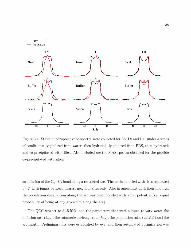
38
Figure 3.4: Static quadrupolar echo spectra were collected for L5, L8 and L11 under a series
of conditions: lyophilized from water, then hydrated; lyophilized from PBS, then hydrated;
and co-precipitated with silica. Also included are the MAS spectra obtained for the peptide
co-precipitated with silica.
as diffusion of the Cγ−Cδ bond along a restricted arc. The arc is modeled with sites separated
by 5 with jumps between nearest neighbor sites only. Also in agreement with their findings,
the population distribution along the arc was best modeled with a flat potential (i.e. equal
probability of being at any given site along the arc).
The QCC was set to 51.5 kHz, and the parameters that were allowed to vary were: the
diffusion rate (karc), the rotameric exchange rate (krot), the population ratio (w:1:1:1) and the
arc length. Preliminary fits were established by eye, and then automated optimization was
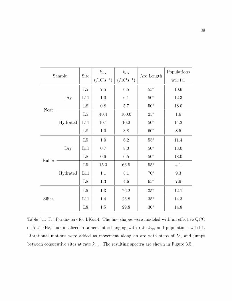
39
Sample Sitekarc krot
Arc LengthPopulations
(/107s−1) (/104s−1) w:1:1:1
Neat
Dry
L5 7.5 6.5 55 10.6
L11 1.0 6.1 50 12.3
L8 0.8 5.7 50 18.0
Hydrated
L5 40.4 100.0 25 1.6
L11 10.1 10.2 50 14.2
L8 1.0 3.8 60 8.5
Buffer
Dry
L5 1.0 6.2 55 11.4
L11 0.7 8.0 50 18.0
L8 0.6 6.5 50 18.0
Hydrated
L5 15.3 66.5 55 4.1
L11 1.1 8.1 70 9.3
L8 1.3 4.6 65 7.9
Silica
L5 1.3 26.2 35 12.1
L11 1.4 26.8 35 14.3
L8 1.5 29.8 30 14.8
Table 3.1: Fit Parameters for LKα14. The line shapes were modeled with an effective QCC
of 51.5 kHz, four idealized rotamers interchanging with rate krot and populations w:1:1:1.
Librational motions were added as movement along an arc with steps of 5, and jumps
between consecutive sites at rate karc. The resulting spectra are shown in Figure 3.5.
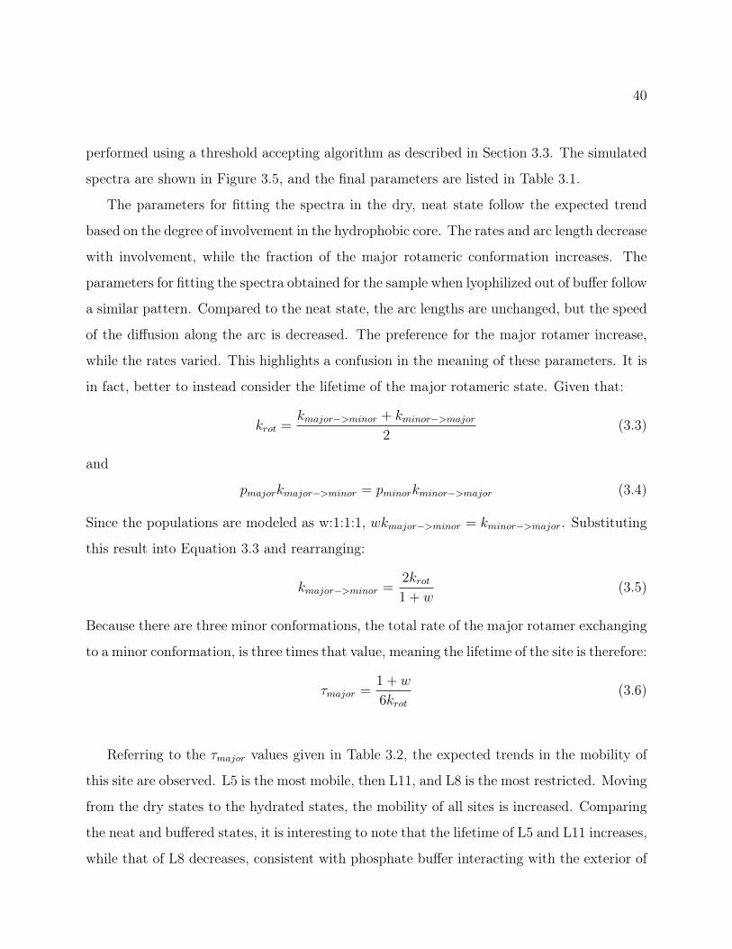
40
performed using a threshold accepting algorithm as described in Section 3.3. The simulated
spectra are shown in Figure 3.5, and the final parameters are listed in Table 3.1.
The parameters for fitting the spectra in the dry, neat state follow the expected trend
based on the degree of involvement in the hydrophobic core. The rates and arc length decrease
with involvement, while the fraction of the major rotameric conformation increases. The
parameters for fitting the spectra obtained for the sample when lyophilized out of buffer follow
a similar pattern. Compared to the neat state, the arc lengths are unchanged, but the speed
of the diffusion along the arc is decreased. The preference for the major rotamer increase,
while the rates varied. This highlights a confusion in the meaning of these parameters. It is
in fact, better to instead consider the lifetime of the major rotameric state. Given that:
krot =kmajor−>minor + kminor−>major
2(3.3)
and
pmajorkmajor−>minor = pminorkminor−>major (3.4)
Since the populations are modeled as w:1:1:1, wkmajor−>minor = kminor−>major. Substituting
this result into Equation 3.3 and rearranging:
kmajor−>minor =2krot1 + w
(3.5)
Because there are three minor conformations, the total rate of the major rotamer exchanging
to a minor conformation, is three times that value, meaning the lifetime of the site is therefore:
τmajor =1 + w
6krot(3.6)
Referring to the τmajor values given in Table 3.2, the expected trends in the mobility of
this site are observed. L5 is the most mobile, then L11, and L8 is the most restricted. Moving
from the dry states to the hydrated states, the mobility of all sites is increased. Comparing
the neat and buffered states, it is interesting to note that the lifetime of L5 and L11 increases,
while that of L8 decreases, consistent with phosphate buffer interacting with the exterior of
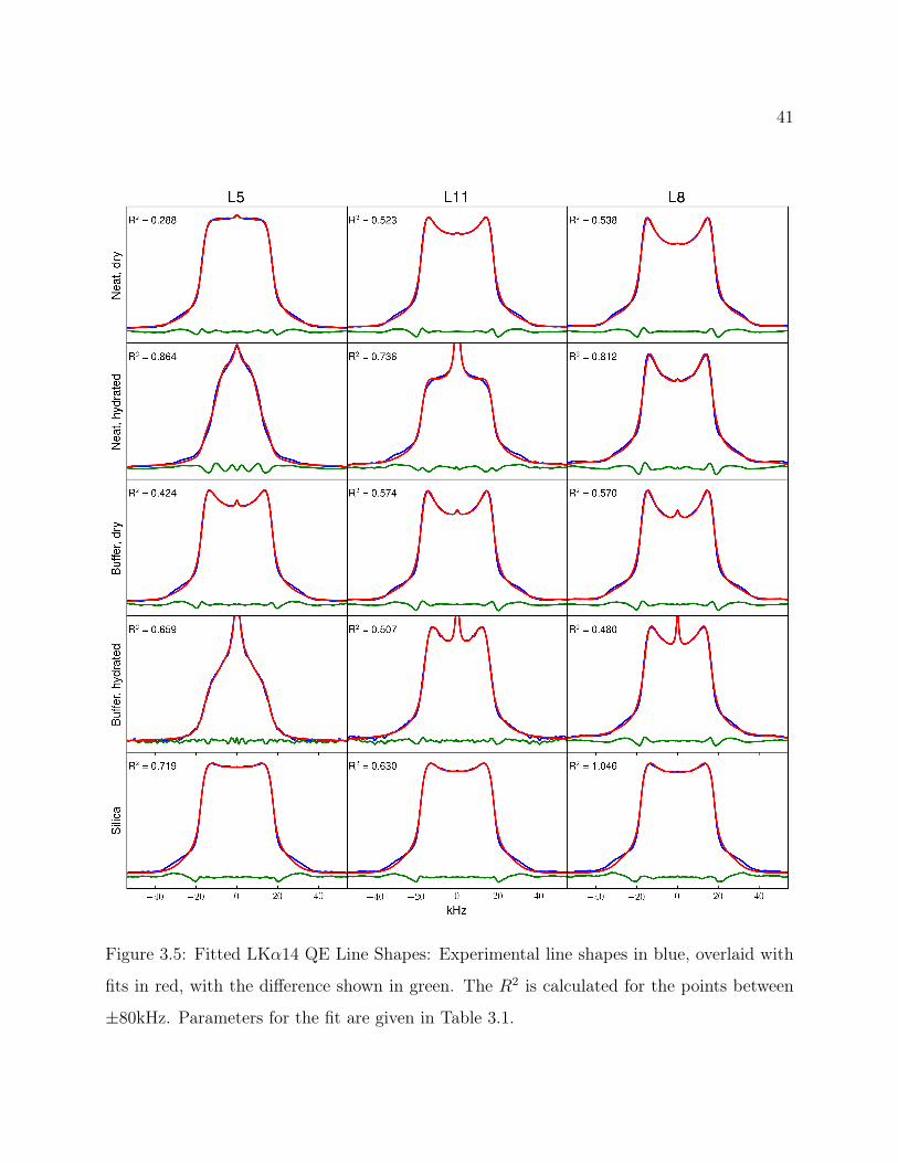
41
Figure 3.5: Fitted LKα14 QE Line Shapes: Experimental line shapes in blue, overlaid with
fits in red, with the difference shown in green. The R2 is calculated for the points between
±80kHz. Parameters for the fit are given in Table 3.1.
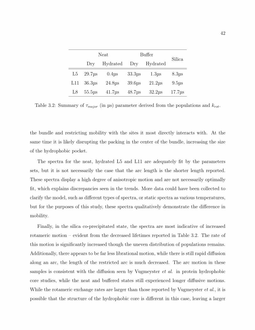
42
Neat BufferSilica
Dry Hydrated Dry Hydrated
L5 29.7µs 0.4µs 33.3µs 1.3µs 8.3µs
L11 36.3µs 24.8µs 39.6µs 21.2µs 9.5µs
L8 55.5µs 41.7µs 48.7µs 32.2µs 17.7µs
Table 3.2: Summary of τmajor (in µs) parameter derived from the populations and krot.
the bundle and restricting mobility with the sites it most directly interacts with. At the
same time it is likely disrupting the packing in the center of the bundle, increasing the size
of the hydrophobic pocket.
The spectra for the neat, hydrated L5 and L11 are adequately fit by the parameters
sets, but it is not necessarily the case that the arc length is the shorter length reported.
These spectra display a high degree of anisotropic motion and are not necessarily optimally
fit, which explains discrepancies seen in the trends. More data could have been collected to
clarify the model, such as different types of spectra, or static spectra as various temperatures,
but for the purposes of this study, these spectra qualitatively demonstrate the difference in
mobility.
Finally, in the silica co-precipitated state, the spectra are most indicative of increased
rotameric motion – evident from the decreased lifetimes reported in Table 3.2. The rate of
this motion is significantly increased though the uneven distribution of populations remains.
Additionally, there appears to be far less librational motion, while there is still rapid diffusion
along an arc, the length of the restricted arc is much decreased. The arc motion in these
samples is consistent with the diffusion seen by Vugmeyster et al. in protein hydrophobic
core studies, while the neat and buffered states still experienced longer diffusive motions.
While the rotameric exchange rates are larger than those reported by Vugmeyster et al., it is
possible that the structure of the hydrophobic core is different in this case, leaving a larger
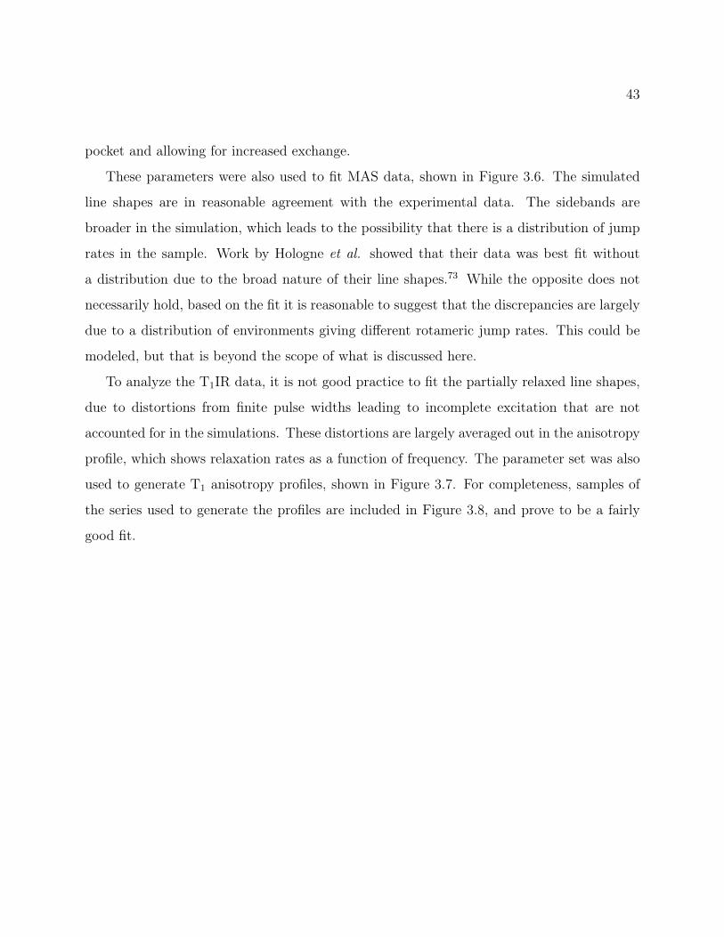
43
pocket and allowing for increased exchange.
These parameters were also used to fit MAS data, shown in Figure 3.6. The simulated
line shapes are in reasonable agreement with the experimental data. The sidebands are
broader in the simulation, which leads to the possibility that there is a distribution of jump
rates in the sample. Work by Hologne et al. showed that their data was best fit without
a distribution due to the broad nature of their line shapes.73 While the opposite does not
necessarily hold, based on the fit it is reasonable to suggest that the discrepancies are largely
due to a distribution of environments giving different rotameric jump rates. This could be
modeled, but that is beyond the scope of what is discussed here.
To analyze the T1IR data, it is not good practice to fit the partially relaxed line shapes,
due to distortions from finite pulse widths leading to incomplete excitation that are not
accounted for in the simulations. These distortions are largely averaged out in the anisotropy
profile, which shows relaxation rates as a function of frequency. The parameter set was also
used to generate T1 anisotropy profiles, shown in Figure 3.7. For completeness, samples of
the series used to generate the profiles are included in Figure 3.8, and prove to be a fairly
good fit.
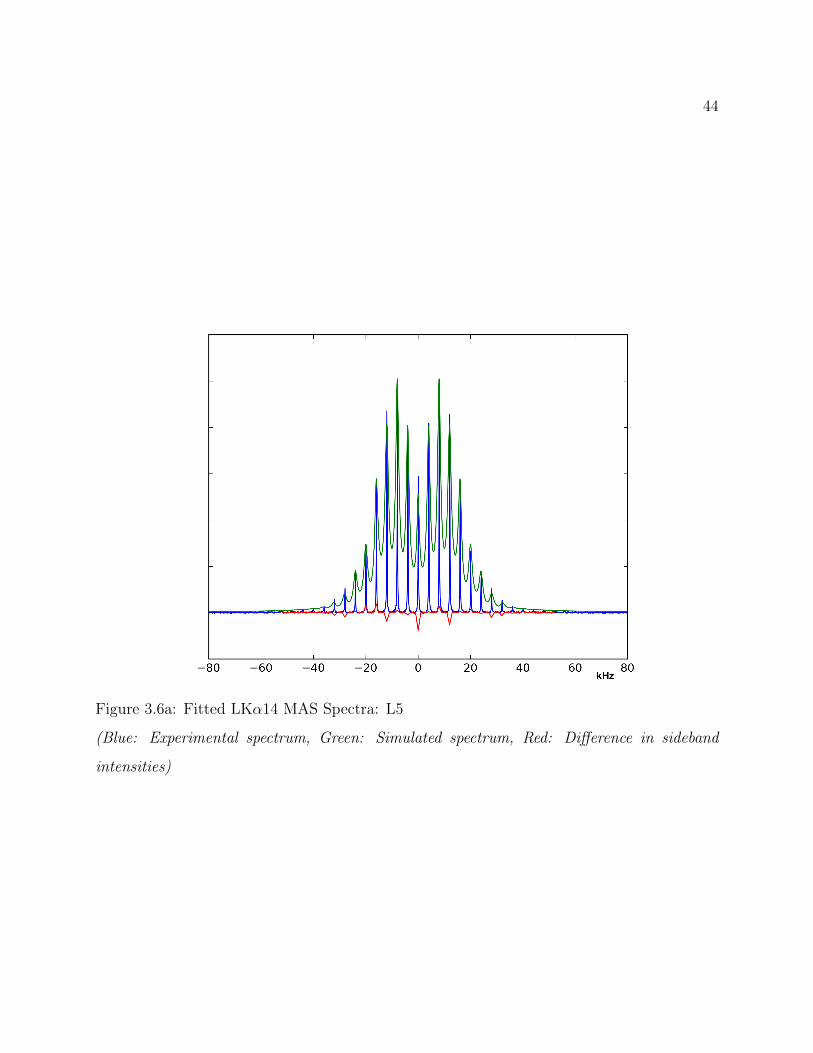
44
Figure 3.6a: Fitted LKα14 MAS Spectra: L5
(Blue: Experimental spectrum, Green: Simulated spectrum, Red: Difference in sideband
intensities)

45
Figure 3.6b: (continued) L11
(Blue: Experimental spectrum, Green: Simulated spectrum, Red: Difference in sideband
intensities)
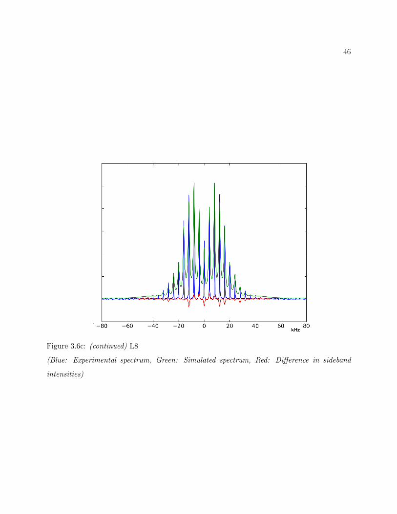
46
Figure 3.6c: (continued) L8
(Blue: Experimental spectrum, Green: Simulated spectrum, Red: Difference in sideband
intensities)

47
Figure 3.7: Fitted LKα14 T1Z Anisotropy Profiles. (Black Line: Static line shape, included
for reference, Blue circles: Experimental Anisotropy, error shown by Grey overlay, Red Line:
Simulated Anisotropy)
Figure 3.8a: LKα14 T1Z partially relaxed line shapes were used to generate the T1Z
Anisotropy Profiles, and are included here for reference. These are not fit directly to avoid
complications of finite pulse width distortions.
L5
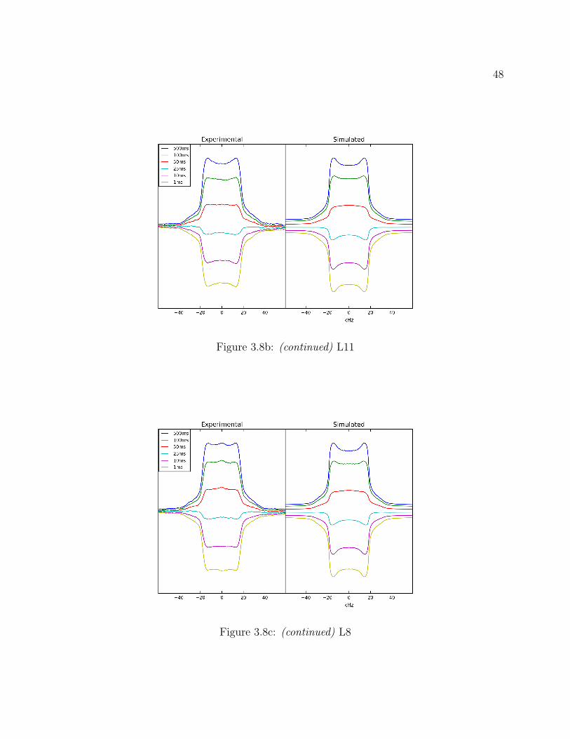
48
Figure 3.8b: (continued) L11
Figure 3.8c: (continued) L8

49
3.7 Conclusions
Static line shapes followed the expected trends of a tetrameric bundle in the neat and buffered
states, with the degree of mobility decreasing with increased involvement in the hydrophobic
core of the proposed tetrameric bundle.48–50 The addition of the buffer increases the mobility
of L8, while decreasing that of L5 and L11. The interactions of the lysine with the phosphate
would introduce steric hindrance to the more exposed sites, and disruption of the packing
would increase the size of the hydrophobic core region.
In the silica co-precipitated state, the trend was still present, though less apparent, and
the spectra demonstrated features consistent with increased rotameric motion and decreased
librational motion. The arc motion is more consistent with the diffusion seen by Vugmeyster
et al. in protein hydrophobic core studies. The replacement of water with silica surrounding
the tetrameric bundles could alleviate the hydrophobic pressure, loosening the packing in the
hydrophobic core and allowing for rotameric exchange. Additionally, the MAS data suggests
that there is a distribution of environments and rates present, the modeling of which is not
attempted here and could be pursued in the future. Data collection at multiple temperatures
would also give better insight into the motional modes present.
Based on this series of spectra, it is likely that the peptide remains in the tetrameric
bundle. The leucine still appears to be in a hydrophobic core environment and there is no
sign of disruption of this packing in the series of spectra presented. This means it is unlikely
that the peptide packing rearranged from the preferred tetrameric bundling.
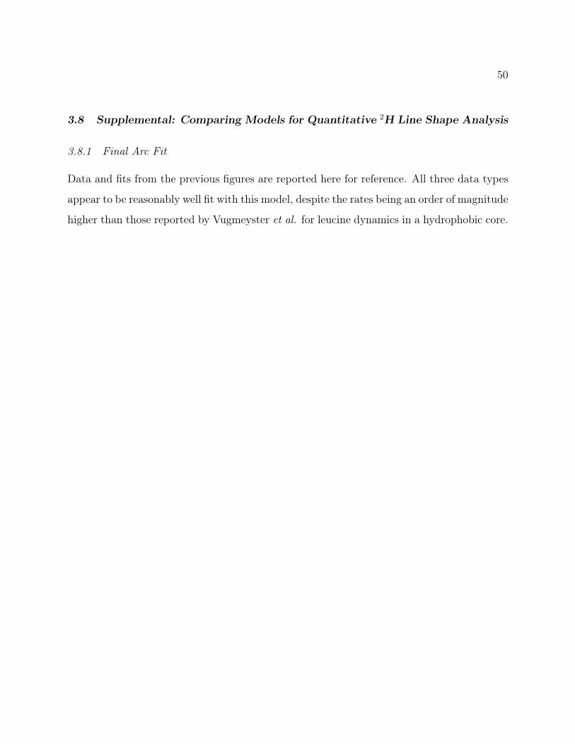
50
3.8 Supplemental: Comparing Models for Quantitative 2H Line Shape Analysis
3.8.1 Final Arc Fit
Data and fits from the previous figures are reported here for reference. All three data types
appear to be reasonably well fit with this model, despite the rates being an order of magnitude
higher than those reported by Vugmeyster et al. for leucine dynamics in a hydrophobic core.
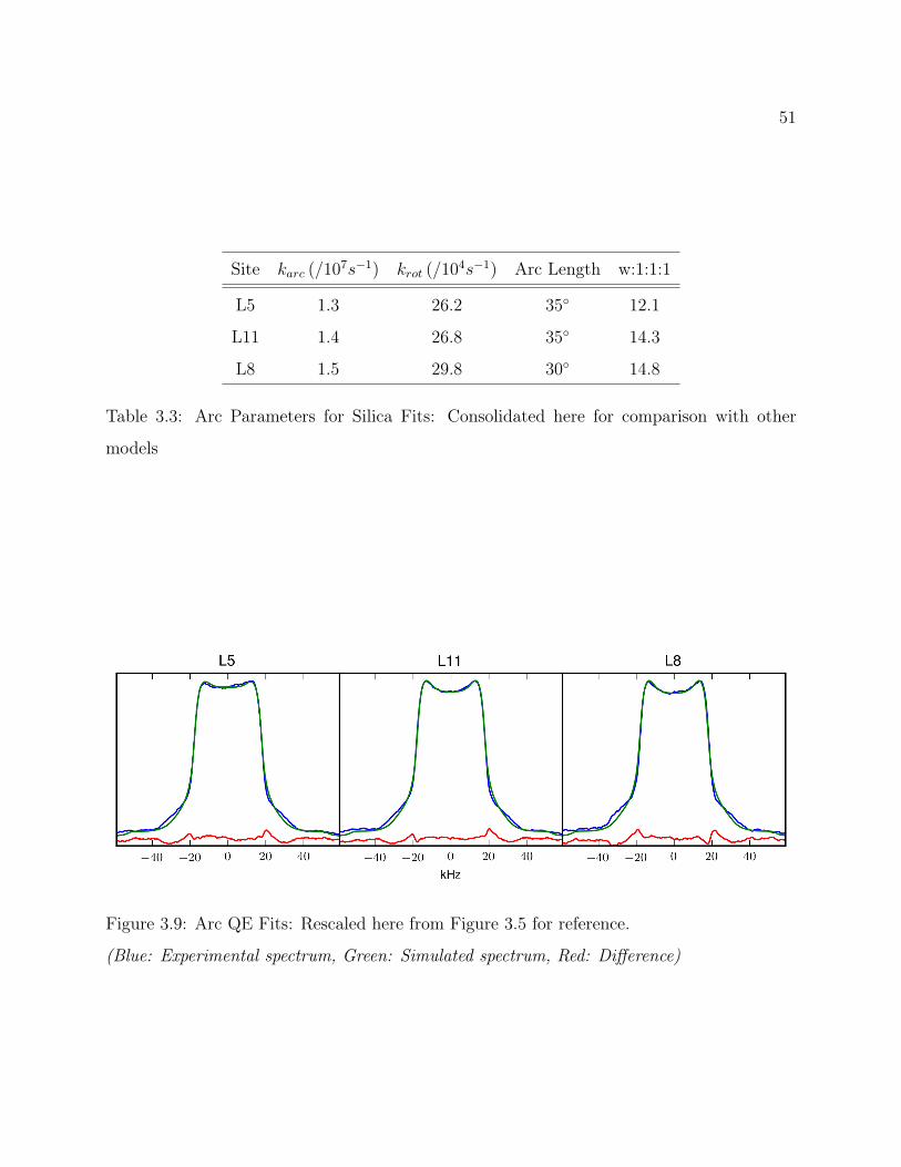
51
Site karc (/107s−1) krot (/104s−1) Arc Length w:1:1:1
L5 1.3 26.2 35 12.1
L11 1.4 26.8 35 14.3
L8 1.5 29.8 30 14.8
Table 3.3: Arc Parameters for Silica Fits: Consolidated here for comparison with other
models
Figure 3.9: Arc QE Fits: Rescaled here from Figure 3.5 for reference.
(Blue: Experimental spectrum, Green: Simulated spectrum, Red: Difference)

52
Figure 3.10: Arc MAS Fits: Rescaled here for easy reference and comparison to alternate
models tried.
(Blue: Experimental spectrum, Green: Simulated spectrum, Red: Difference in sideband
intensities)
Figure 3.11: Arc T1 Fits: Reproduced here for easy reference and comparison to alternate
models tried.
(Black Line: Static line shape, included for reference, Blue circles: Experimental Anisotropy,
error shown by Grey overlay, Red Line: Simulated Anisotropy)

53
3.8.2 Alternate Arc Fit
Presented here is an alternate parameter set, using the same 4-rotamer + variable length arc
model that was used to fit the data. The rotamer exchange rates were constrained to be on
the order of 104s−1, to be closer to the values reported by Vugmeyster et al.. The parameters
for this fit are presented in Table 3.4. Overall, fitting the QE spectra with a decreased krot
lead to a model with an increased karc, and arc length, that is, faster librational movement
along a longer trajectory. Additionally there is an overall increase in the w:1:1:1 ratio,
indicating a prediction of increased steric hindrance relative to the first model.
The QE fits using this model, shown in Figure 3.12, appear to do a better job of fitting
the shoulder region of the spectrum, and based on that alone may lead one to believe it is in
fact a better fit. However, MAS spectra simulated from this model show significant side band
broadening, shown in Figure 3.13, and the discrepancy between that and the experimental
data is an indicator that it is not a good fit. Furthermore, the T1 anisotropy profiles, shown
in Figure 3.14, are not as close a fit as those shown in Figure 3.11.
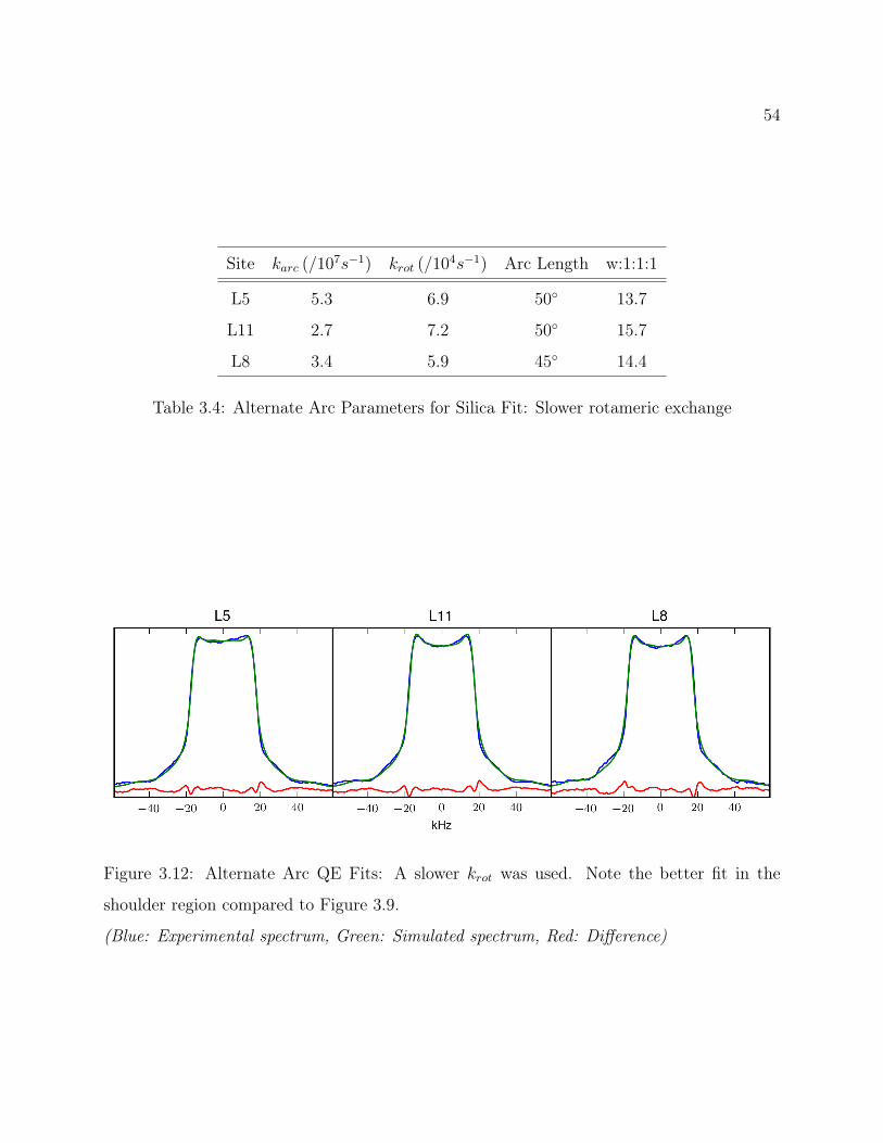
54
Site karc (/107s−1) krot (/104s−1) Arc Length w:1:1:1
L5 5.3 6.9 50 13.7
L11 2.7 7.2 50 15.7
L8 3.4 5.9 45 14.4
Table 3.4: Alternate Arc Parameters for Silica Fit: Slower rotameric exchange
Figure 3.12: Alternate Arc QE Fits: A slower krot was used. Note the better fit in the
shoulder region compared to Figure 3.9.
(Blue: Experimental spectrum, Green: Simulated spectrum, Red: Difference)
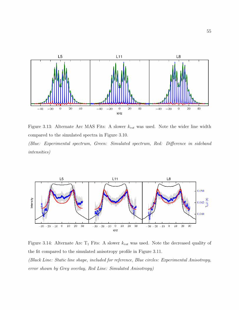
55
Figure 3.13: Alternate Arc MAS Fits: A slower krot was used. Note the wider line width
compared to the simulated spectra in Figure 3.10.
(Blue: Experimental spectrum, Green: Simulated spectrum, Red: Difference in sideband
intensities)
Figure 3.14: Alternate Arc T1 Fits: A slower krot was used. Note the decreased quality of
the fit compared to the simulated anisotropy profile in Figure 3.11.
(Black Line: Static line shape, included for reference, Blue circles: Experimental Anisotropy,
error shown by Grey overlay, Red Line: Simulated Anisotropy)
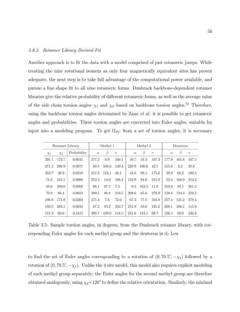
56
3.8.3 Rotamer Library Derived Fit
Another approach is to fit the data with a model comprised of just rotameric jumps. While
treating the nine rotational isomers as only four magnetically equivalent sites has proven
adequate, the next step is to take full advantage of the computational power available, and
pursue a line shape fit to all nine rotameric forms. Dunbrack backbone-dependent rotamer
libraries give the relative probability of different rotameric forms, as well as the average value
of the side chain torsion angles–χ1 and χ2–based on backbone torsion angles.74 Therefore,
using the backbone torsion angles determined by Zane et al. it is possible to get rotameric
angles and probabilities. These torsion angles are converted into Euler angles, suitable for
input into a modeling program. To get ΩPC from a set of torsion angles, it is necessary
Rotamer Library Methyl 1 Methyl 2 Deuteron
χ1 χ2 Probability α β γ α β γ α β γ
291.1 172.7 0.6045 271.2 6.9 340.1 59.7 34.3 167.3 177.9 165.8 347.5
271.1 298.9 0.0071 60.5 108.6 149.4 228.9 100.6 42.5 155.8 6.1 35.6
263.7 40.9 0.0210 311.8 124.1 48.1 44.5 89.1 175.6 28.9 66.2 100.5
74.3 165.1 0.0000 272.5 14.0 198.2 132.9 84.6 315.8 52.4 168.9 213.2
58.6 286.0 0.0000 66.1 97.7 7.5 9.4 162.5 11.9 359.8 50.1 261.2
70.0 86.4 0.0024 289.5 86.8 219.5 209.6 65.0 278.9 128.8 124.4 259.2
198.8 171.9 0.0203 271.4 7.6 72.6 67.3 77.5 316.9 257.4 121.2 278.4
193.5 283.1 0.0033 67.2 95.2 233.7 251.8 53.6 191.6 208.1 166.1 115.9
181.2 60.6 0.3413 299.7 109.0 118.5 251.6 124.1 69.7 198.4 88.0 330.8
Table 3.5: Sample torsion angles, in degrees, from the Dunbrack rotamer library, with cor-
responding Euler angles for each methyl group and the deuteron in d7 Leu
to find the set of Euler angles corresponding to a rotation of (0, 70.5°,−χ2) followed by a
rotation of (0, 70.5°,−χ1). Unlike the 4 site model, this model also requires explicit modeling
of each methyl group separately; the Euler angles for the second methyl group are therefore
obtained analogously, using χ2+120° to define the relative orientation. Similarly, the minimal

57
contribution of the Cγ deuteron–appearing as a baseline increase with < 5% contribution,
due to signal attenuation because of the longer relaxation time–is accounted for by adjusting
χ2 to χ2 − 120°. Sample rotamer library data with corresponding rotation angles, is shown
in Table 3.5. It is also worth mentioning that of the 9 sites, three of them are likely able
to be eliminated from consideration, as the projected populations are < 1%. The reason
for this becomes evident when looking at the three dimensional structure, as the gauche(-
) configuration of χ1 directs the side chain back towards the helical backbone, which is a
sterically unfavorable position.
Using torsion angles from the Dunbrack rotamer libraries, the spectra were simulated
using just jumps between six of the nine possible rotameric conformations. The QCC was
allowed to vary, as well at the populations of all six rotamers and three jump rates cor-
responding to changes in χ1, χ2 and both χ1 and χ2. The results are presented in Table
3.6. While in an ideal case, this model would have given us results that are more physically
meaningful due to the accurate representation of all the rotameric contributions, in reality
the results were less than ideal. It ultimately seemed that the complication of the model
added too many parameters for the results to lead to meaningful physical conclusions.

58
Site k1 (s−1) k2 (s−1) k12 (s−1) QCCeff (kHz) p1 p2 p3 p4 p5 p6
L5 41.9 10.4 3.78× 10⁵ 48.6 0.767 0.073 0.020 0.093 0.046 0.0001
L11 7.2 5.0 3.55× 10⁵ 48.7 0.727 0.062 0.025 0.153 0.0331 10−8
L8 10.8 8.3 4.12× 10⁵ 48.8 0.730 0.044 0.031 0.165 0.030 10−8
Table 3.6: Rotamer-Only Parameters for Silica Fit
Figure 3.15a: Rotamer-Only QE Fits: The "horn" region is not as closely fit, and required
a water peak in the center to account for some of the spectral intensity.
(Blue: Experimental spectrum, Green: Simulated spectrum, Red: Difference)
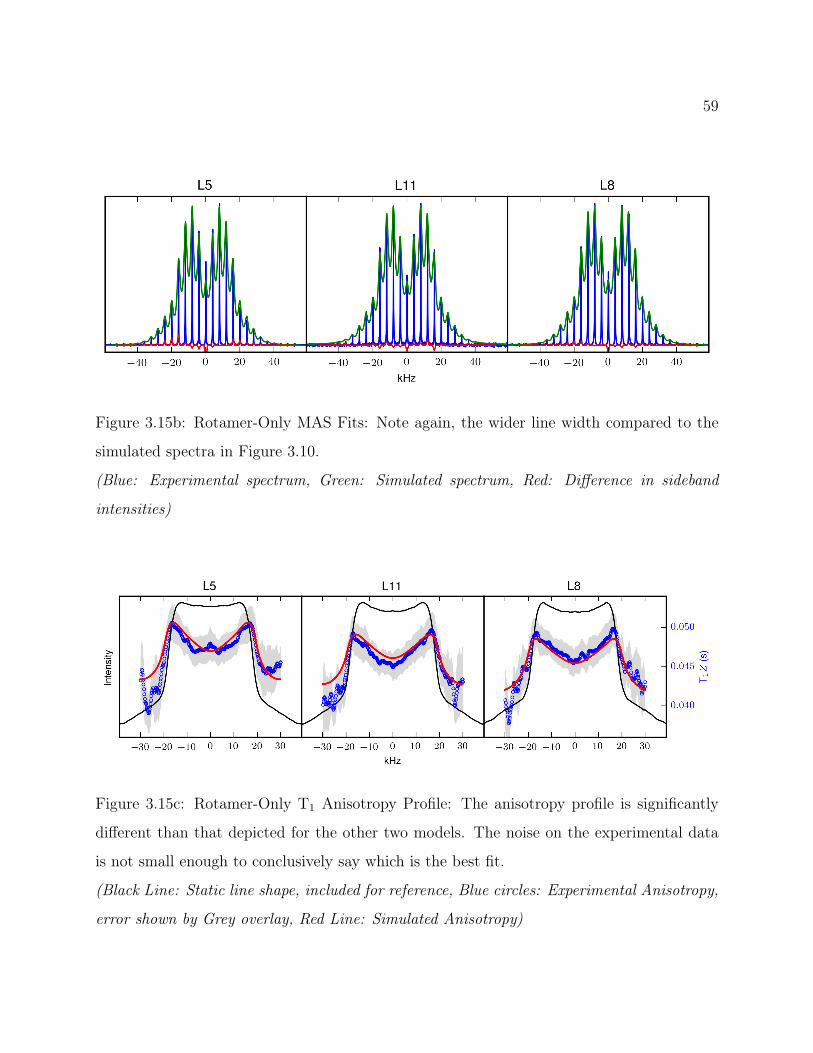
59
Figure 3.15b: Rotamer-Only MAS Fits: Note again, the wider line width compared to the
simulated spectra in Figure 3.10.
(Blue: Experimental spectrum, Green: Simulated spectrum, Red: Difference in sideband
intensities)
Figure 3.15c: Rotamer-Only T1 Anisotropy Profile: The anisotropy profile is significantly
different than that depicted for the other two models. The noise on the experimental data
is not small enough to conclusively say which is the best fit.
(Black Line: Static line shape, included for reference, Blue circles: Experimental Anisotropy,
error shown by Grey overlay, Red Line: Simulated Anisotropy)

60
Chapter 4
ISOLEUCINE DYNAMICS AND 2H-13C HETERONUCLEARCORRELATION NMR
4.1 Introduction
4.1.1 An extension of leucine dynamics
Having demonstrated the efficacy of extracting motional information from 2H ssNMR data
for leucine side chains, it seems a logical follow up to apply it to other amino acids. Isoleucine
is another hydrophobic amino acid with potentially interesting methyl group dynamics. How-
ever, while there is a wealth of leucine dynamics literature, there is a paucity of analogous
isoleucine analysis. In a study of amino acid side chain motions through relaxation ex-
periments, Oldfield et al., states that due to its complicated structure, shown in Figure
4.1, isoleucine requires further study to properly model.75 Follow up studies are few in
number, and include a method of solution state χ2 determination, using 13C CPMG (Car-
Purcell-Meiboom-Gill) relaxation dispersion–which has been used to analyze both leucine
and isoleucine conformational exchange.76,77
HO
C
O
CαD
NH2
CβD
Cγ2D3
Cγ1D2
CδD3
Figure 4.1: Structure of d10 isoleucine.

61
The structure of isoleucine, shown in Figure 4.1, is asymmetric, leading to two inequiva-
lent methyl group environments. The inequivalent methyl groups complicate the line shape.
While leucine can be purchase with d7 − isopropyl, d3 −methyl and d10 labeling, isoleucine
with 2H labeling is available for purchase only in the perdeuterated form, meaning that all
10 hydrogen atoms are replaced with deuterium, as shown in Figure 4.1. Since selectively
labeled material is not readily available, the motions along the side chain cannot be exam-
ined separately. The resulting line shape includes not only the contributions from the two
non-equivalent methyl groups, but also broader line shapes corresponding to the deuterons
at the α, β and γ positions.
4.1.2 Applications
If this analysis method proves successful, this technique could then be applied to isoleucine
dynamics with the amino acid incorporated into a peptide sequence. A potential example
is R5 (H-SSKKSGSYSGSKGSKRRIL-OH), another synthetic silaffin, which is capable of
silica precipitation.13,14,78 This is particularly interesting because the RRIL moiety has been
shown to be important to silica morphology mediation.14,78 The leucine is hard to label
because in solid-phase peptide synthesis, the C-terminal amino acid is bound to a resin,
and so is more difficult to isotopically label. Therefore, it would be advantageous to have a
method for evaluating the dynamics of the isoleucine side chain instead.
4.1.3 Methods
Building upon the techniques for leucine dynamics modeling presented in Chapter 3, a similar
analysis is done on isoleucine spectra by modeling an overall spectrum as the sum of each site’s
contribution. To further verify the veracity of this method it is desirable to have a method of
separating out these contributions. The broader deuteron contributions can be reduced by
decreasing the recycle delay, shown in Figure 4.2, but it is preferable to separate out these
motions entirely. To this end, 2H-13C heteronuclear correlation (HETCOR) spectroscopy
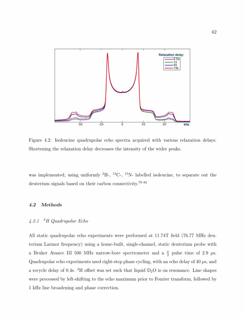
62
Figure 4.2: Isoleucine quadrupolar echo spectra acquired with various relaxation delays.
Shortening the relaxation delay decreases the intensity of the wider peaks.
was implemented, using uniformly 2H-, 13C-, 15N- labelled isoleucine, to separate out the
deuterium signals based on their carbon connectivity.79–82
4.2 Methods
4.2.1 2H Quadrupolar Echo
All static quadrupolar echo experiments were performed at 11.74T field (76.77 MHz deu-
terium Larmor frequency) using a home-built, single-channel, static deuterium probe with
a Bruker Avance III 500 MHz narrow-bore spectrometer and a π2
pulse time of 2.9 µs.
Quadrupolar echo experiments used eight-step phase cycling, with an echo delay of 40 µs, and
a recycle delay of 0.4s. 2H offset was set such that liquid D2O is on resonance. Line shapes
were processed by left-shifting to the echo maximum prior to Fourier transform, followed by
1 kHz line broadening and phase correction.
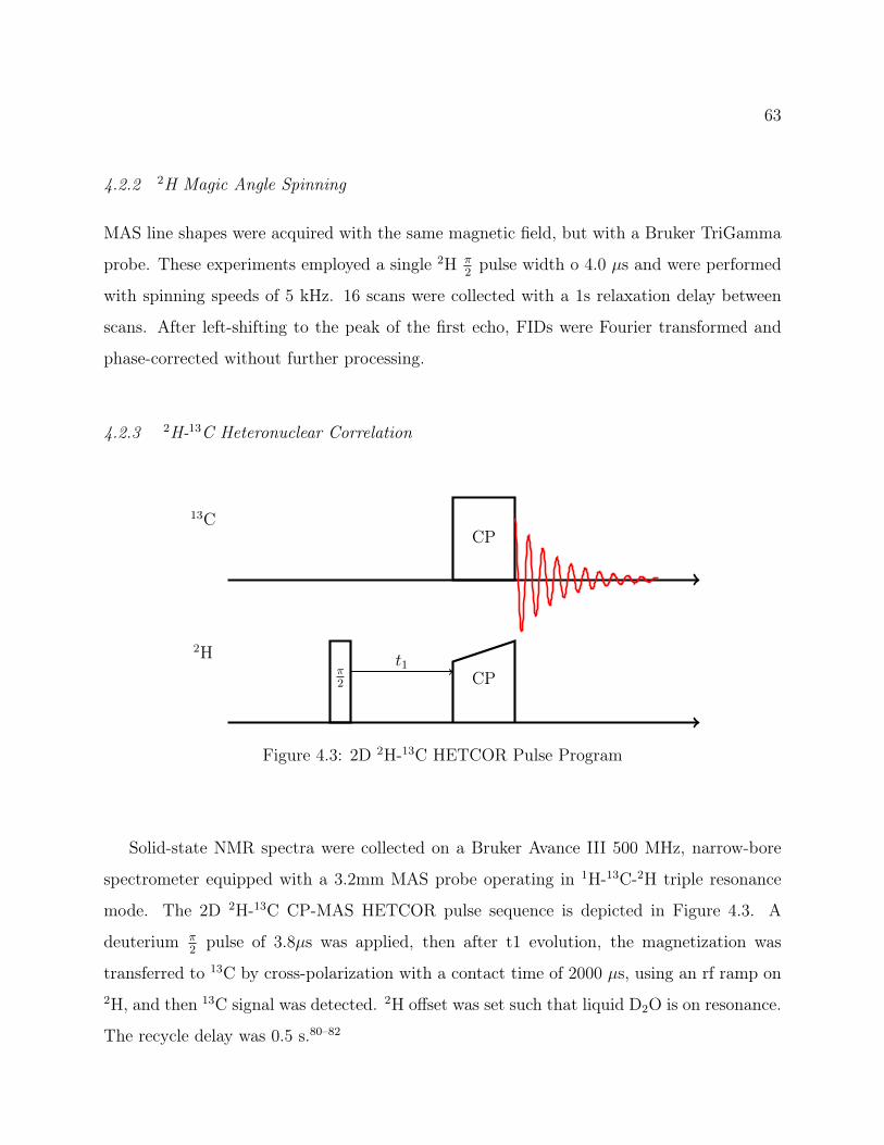
63
4.2.2 2H Magic Angle Spinning
MAS line shapes were acquired with the same magnetic field, but with a Bruker TriGamma
probe. These experiments employed a single 2H π2pulse width o 4.0 µs and were performed
with spinning speeds of 5 kHz. 16 scans were collected with a 1s relaxation delay between
scans. After left-shifting to the peak of the first echo, FIDs were Fourier transformed and
phase-corrected without further processing.
4.2.3 2H-13C Heteronuclear Correlation
2Hπ2
t1CP
13CCP
Figure 4.3: 2D 2H-13C HETCOR Pulse Program
Solid-state NMR spectra were collected on a Bruker Avance III 500 MHz, narrow-bore
spectrometer equipped with a 3.2mm MAS probe operating in 1H-13C-2H triple resonance
mode. The 2D 2H-13C CP-MAS HETCOR pulse sequence is depicted in Figure 4.3. A
deuterium π2pulse of 3.8µs was applied, then after t1 evolution, the magnetization was
transferred to 13C by cross-polarization with a contact time of 2000 µs, using an rf ramp on2H, and then 13C signal was detected. 2H offset was set such that liquid D2O is on resonance.
The recycle delay was 0.5 s.80–82

64
13C Chemical Shift (ppm)
2H
Chemical
Shift
(ppm
)
Figure 4.4: An overview of the 2D 2H-13C CP-MAS HETCOR. Spectral width was 50 kHz
for 13C and 500 kHz for 2H, a total of 4096 t1 increments with 4 scans each were collected.
4.3 Results
The overall 2D HETCOR spectrum is shown in Figure 4.4, with peak assignments for the 13C
shifts given in Figure 4.5. Peaks assignments are based on literature work, which determined
that the two different rotameric populations in monomeric isoleucine, g+t and tt,83 lead to
inequivalent environments for Cγ2H3 and two different chemical shifts in the 13C spectrum.84
Interestingly, the dominate forms reported by the Dynameomics rotamer library are g+t and
g−t, indicating a difference based on protein incorporation.85
4.3.1 Model
Taking inspiration from past work by Vugmeyster et al., the data was fit using a simple arc
motion, treated as a rotation of the Cα−Cβ bond, causing the rest of the molecule to rapidly
diffuse along a restricted arc with a length of 30, jumping steps of 5 at a rate of 5×10⁸s−1.
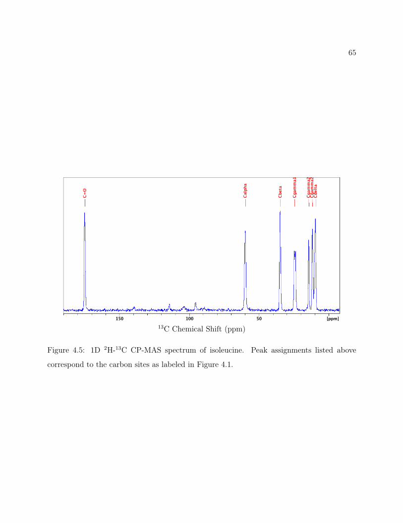
65
13C Chemical Shift (ppm)
Figure 4.5: 1D 2H-13C CP-MAS spectrum of isoleucine. Peak assignments listed above
correspond to the carbon sites as labeled in Figure 4.1.
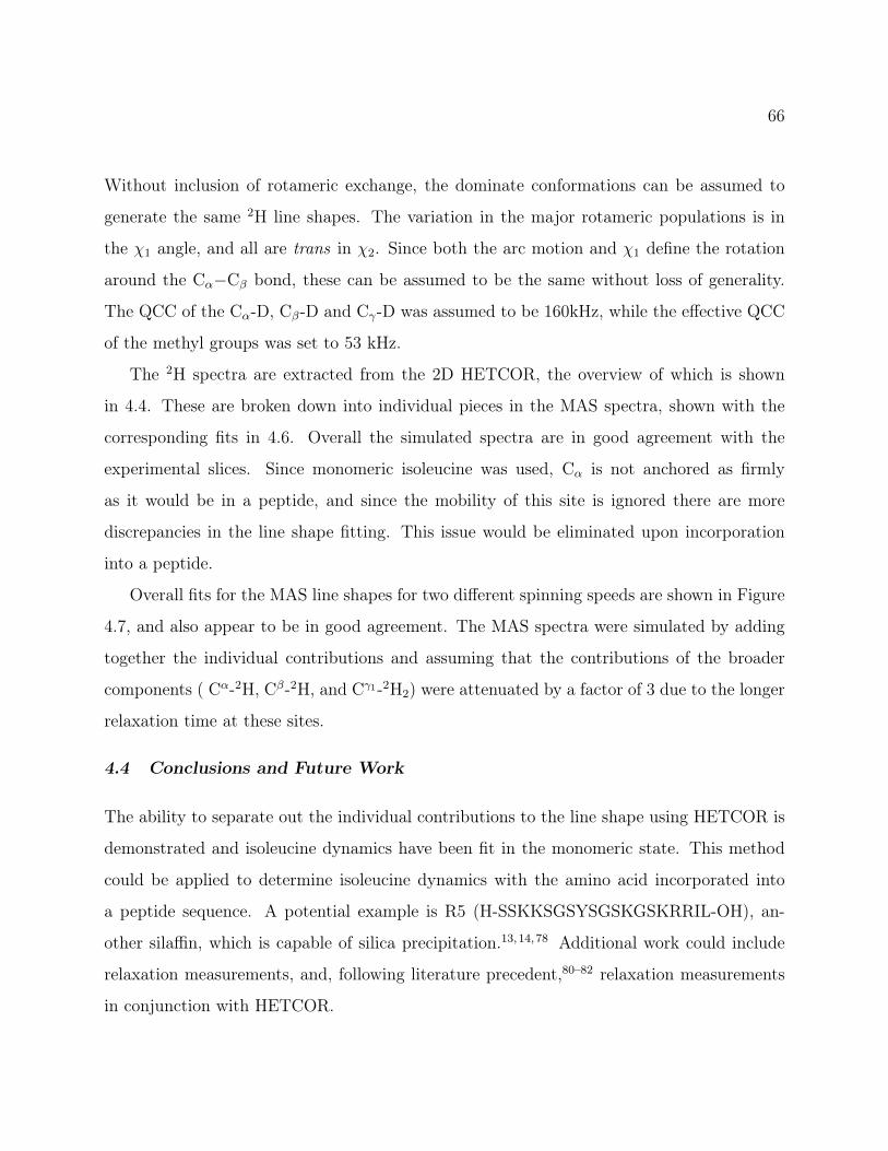
66
Without inclusion of rotameric exchange, the dominate conformations can be assumed to
generate the same 2H line shapes. The variation in the major rotameric populations is in
the χ1 angle, and all are trans in χ2. Since both the arc motion and χ1 define the rotation
around the Cα−Cβ bond, these can be assumed to be the same without loss of generality.
The QCC of the Cα-D, Cβ-D and Cγ-D was assumed to be 160kHz, while the effective QCC
of the methyl groups was set to 53 kHz.
The 2H spectra are extracted from the 2D HETCOR, the overview of which is shown
in 4.4. These are broken down into individual pieces in the MAS spectra, shown with the
corresponding fits in 4.6. Overall the simulated spectra are in good agreement with the
experimental slices. Since monomeric isoleucine was used, Cα is not anchored as firmly
as it would be in a peptide, and since the mobility of this site is ignored there are more
discrepancies in the line shape fitting. This issue would be eliminated upon incorporation
into a peptide.
Overall fits for the MAS line shapes for two different spinning speeds are shown in Figure
4.7, and also appear to be in good agreement. The MAS spectra were simulated by adding
together the individual contributions and assuming that the contributions of the broader
components ( Cα-2H, Cβ-2H, and Cγ1-2H2) were attenuated by a factor of 3 due to the longer
relaxation time at these sites.
4.4 Conclusions and Future Work
The ability to separate out the individual contributions to the line shape using HETCOR is
demonstrated and isoleucine dynamics have been fit in the monomeric state. This method
could be applied to determine isoleucine dynamics with the amino acid incorporated into
a peptide sequence. A potential example is R5 (H-SSKKSGSYSGSKGSKRRIL-OH), an-
other silaffin, which is capable of silica precipitation.13,14,78 Additional work could include
relaxation measurements, and, following literature precedent,80–82 relaxation measurements
in conjunction with HETCOR.
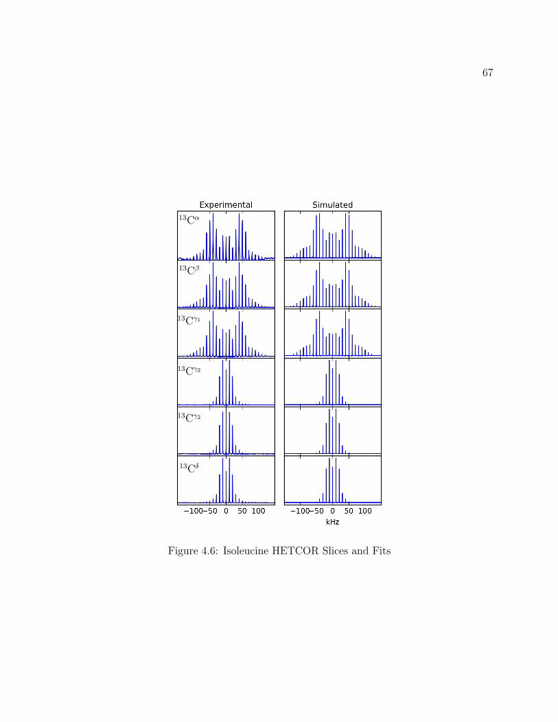
67
13Cα
13Cβ
13Cγ1
13Cγ2
13Cγ2
13Cδ
Figure 4.6: Isoleucine HETCOR Slices and Fits
68
(a) Simulated (b) Experimental
(c) Simulated (d) Experimental
Figure 4.7: Experimental and Simulated MAS Line Shapes for Isoleucine at 5kHz and 10kHz
spin rates.
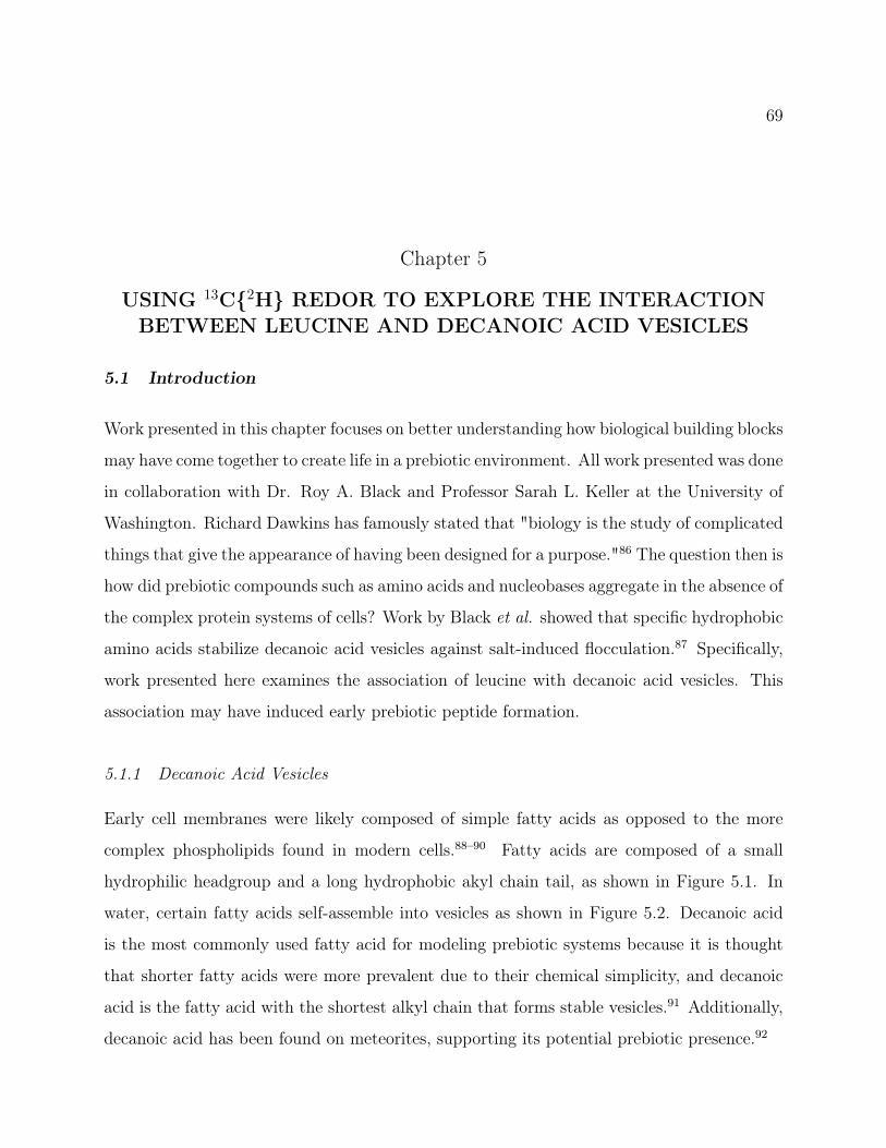
69
Chapter 5
USING 13C2H REDOR TO EXPLORE THE INTERACTIONBETWEEN LEUCINE AND DECANOIC ACID VESICLES
5.1 Introduction
Work presented in this chapter focuses on better understanding how biological building blocks
may have come together to create life in a prebiotic environment. All work presented was done
in collaboration with Dr. Roy A. Black and Professor Sarah L. Keller at the University of
Washington. Richard Dawkins has famously stated that "biology is the study of complicated
things that give the appearance of having been designed for a purpose."86 The question then is
how did prebiotic compounds such as amino acids and nucleobases aggregate in the absence of
the complex protein systems of cells? Work by Black et al. showed that specific hydrophobic
amino acids stabilize decanoic acid vesicles against salt-induced flocculation.87 Specifically,
work presented here examines the association of leucine with decanoic acid vesicles. This
association may have induced early prebiotic peptide formation.
5.1.1 Decanoic Acid Vesicles
Early cell membranes were likely composed of simple fatty acids as opposed to the more
complex phospholipids found in modern cells.88–90 Fatty acids are composed of a small
hydrophilic headgroup and a long hydrophobic akyl chain tail, as shown in Figure 5.1. In
water, certain fatty acids self-assemble into vesicles as shown in Figure 5.2. Decanoic acid
is the most commonly used fatty acid for modeling prebiotic systems because it is thought
that shorter fatty acids were more prevalent due to their chemical simplicity, and decanoic
acid is the fatty acid with the shortest alkyl chain that forms stable vesicles.91 Additionally,
decanoic acid has been found on meteorites, supporting its potential prebiotic presence.92
70
The vesicles formed by decanoic acid create a small hydrophobic sheet, as well as an
inner pocket of aqueous solution. Both of these features may have led to the aggregation of
prebiotic components, an essential first step in the formation of more complicated molecules.
Roy Black et al. have shown that certain RNA bases and ribose bind to decanoic acid
vesicles and stabilize the vesicles against salt-induced flocculation.93 More recently, Black
et al. showed that certain non-polar amino acids, including leucine and isoleucine, are
also able to stabilize vesicles in high salt concentrations. In contrast, alanine and glycine,
which are less hydrophobic, were shown to have little effect on the stability of the fatty acid
vesicles.87 To better understand this preferential stabilization in the presence of leucine, I
employed solid-state NMR techniques to investigate whether leucine binds to the surface or
is incorporated into the core of the bilayer.
5.1.2 13C2H REDOR
Rotational-echo double-resonance (REDOR) NMR spectroscopy is a method for determining
heteronuclear distances in solid samples. This technique is commonly implemented in the
study of systems which are not easily characterized by crystallography. REDOR is routinely
used to measure distances of up to 7 Å between 13C and 15N nuclei in peptide conformational
studies. In a 13CX REDOR experiment, the dipolar dephasing of 13C spins by the other
nucleus, X is monitored. Dipolar coupling is inversely proportional to the cube of the dis-
tances, so at longer distances there is a rapid increase in uncertainty. Here 13C2H REDOR
is employed, in large part due to the availability of selectively deuterated decanoic acid.
The measurement of dephasing as a function of time was accomplished by recording pairs
of spectra at different recoupling times, using the pulse sequence shown in Figure 5.3.94–97
In both spectra, the signal is generated by cross polarization of magnetization from 1H to13C, followed by a series of rotor-synchronized π pulses on the 13C channel to refocus the
magnetization. The S0 is the spectrum recorded without recoupling to 2H, while the S1 is
generated by adding a series of π pulses on the 2H channel interleaved with the refocusing
pulses on the 13C channel. Note that in the case of 2H as the dephasing nucleus, some have

71
opted to use a composite π pulse to ensure inversion of the full signal, however this is not
necessary given a sufficiently hard short π pulse.94–97
From these spectra, the change in intensity, ∆S = S0−S1
S0is determined as a function of
time. This curve is then fit to extract the distance information. Most frequently this data
takes the form of a sigmoidal curve, but in the case of dephasing by 2H, the T1 relaxation
time of the deuterium is short enough that this is not generally seen.97 In an investigation of
peptide insertion into the membrane, it was found that the data was well fit by an exponential
of the form A(1−e−γt), where A is the fraction of molecules with effective carbon-deuterium
coupling d = 3γ2.97 The distance, r, is then calculated as [4642Hz
3γ/2]13 .
To verify that the pulse sequence would result in the desired dephasing, a sample of
methionine-1-13C-methyl-2H3 was used, as was done by Luthra et al.98 The structure of
this compound is shown in Figure 5.4. Since we do not need to quantify distance as they
have done, and simply wanted to verify the relative degree of dephasing, the sample used
was not recrystallized, and was simply lyophilized after dilution with unlabeled methionine
so the sample contained just 10% labeled material to minimize intermolecular interactions.
The clear dephasing is sufficient to confirm the method. The data, plotted in Figure 5.5,
does appear to show exponential behavior, but the fitting according to the method employed
by Weliky et al. yields a effective 13C-2H coupling of 135 Hz, and distance of 4.1 Å. This
is shorter than the 5.98 Å one would expect based on the crystal structure.98 The shorter
distance could be cause by greater disorder in the methionine side chain compared to a neatly
ordered crystal structure.
5.2 Methods
5.2.1 Materials
L-methionine (1-13C; methyl-d3) for control experiment was purchased from Cambridge Iso-
tope Laboratories (Andover, MA). L-Leucine (13C6) and decanoic-10,10,10-d3 acid were pur-
chased from Cambridge Isotope Laboratories (Andover, MA). Decanoic-2,2-d2 acid was pur-

72
chased from C/D/N Isotopes Inc. (Quebec, CA); deuterium depleted water from Sigma-
Aldrich.
5.2.2 Sample Preparation
Sample preparation was performed by Roy Black; the protocol is reported here for reference.
(Note: the masses used here refer to methyl-deuterated decanoic acid (MW 175 g/mol)
and uniformly-13C6 labeled leucine (MW 137 g/mol) and these were adjusted to reflect
the labeling scheme in use.) Decanoic acid (77.7 mg) was heated and vortexed in 1 M
NaOH/deuterium-depleted water (0.524 mL). To this mixture, deuterium-depleted water
(2.323 mL) was added and vortexed resulting in a 161 mM decanoic acid solution. Additional
deuterium-depleted water (3.444 mL) was added and vortexed, diluting the solution to 72
mM. The solution was then titrated to pH 7.5 using HCl solutions made with deuterium
depleted water (approximately 77 µL 6 M HCl, 59 µL 1 M HCl). 3mL of this solution was
then added to 13C leucine (4.1 mg) to make a vesicle sample that is 72 mM decanoic acid,
and 10 mM leucine.
The sample was then lyophilized to a powder for NMR studies.
5.2.3 13C2H REDOR
Experiments were done with a 11.74 T Bruker Avance III 500 MHz, narrow-bore spectrometer
using a Bruker TriGamma probe tuned for 1H-13C-2H triple resonance. Pulse program used
is depicted in Figure 5.3. Samples were spun at 10kHz MAS frequency, S0 and S1 were
collected for dephasing times of 0.8, 3.2, 5.6, 8.0 and 10.4 ms and required 1024, 2048, 2048,
2048 and 4096 scans, respectively. The contact time used in the CP was 1.5 ms, during
this time the 1H power was ramped from 70% to 100%. Field strengths were: 83 kHz 1H π2
pulse, 56 kHz 13C π pulses, and 66 kHz 2H π pulses. During dephasing and decoupling 100
kHz SPINAL-64 decoupling was applied on the 1H channel.99 Data was processed with 20
Hz Gaussian line broadening and baseline correction. Chemical shift referencing was done
externally using adamantane. The methylene 13C shift was set to 38.5 ppm.
73
5.3 Results
To examine the relative location of leucine in the bilayer, selectively labelled decanoic acid
was used. Specifically, for the 13C2H REDOR, the dephasing of 13CO in leucine was
recorded for two different samples of decanoic acid, shown in Figure 5.6. Decanoic-2,2-d2
acid and decanoic-10,10,10-d3 acid were selected to clearly distinguish between association
of leucine near the head group and leucine in the center of the bilayer, respectively.
Figures 5.8 and 5.9 show the carbonyl region of the REDOR S0 and S1, for decanoic-
10,10,10-d3 acid and decanoic-2,2-d2 acid respectively, with 0.8 ms, 3 .2 ms, 5.6 ms, 8.0
ms and 10.4 ms dipolar recoupling periods. There are two peaks for the leucine 13CO, at
177.6 and 176.4 ppm, as reported in the literature.100 These could potentially reflect two
different crystal structure of leucine. Before considering the behavior of the leucine further,
a comment on the other contribution to the spectra. The peak at 182 ppm is from the
natural abundance 13CO in the decanoic acid. This assignment is reinforced by the rapid
dephasing of the peak with the decanoic-2,2-d2 acid sample, as the carbonyl adjacent to the
CD2 group. Note that not all of the decanoic acid will be incorporated into the vesicles, and
this second population is reflected by the presence of a second peak at 184 ppm.
Now, focusing on just the signal from the leucine 13CO, presented in Figures 5.11 and
5.10 for the 3.2 ms, 5.6 ms, 8.0 ms and 10.4 ms dipolar recoupling periods. The leucine 13CO
signal for both samples is broad, reflecting the contributions of the two leucine populations,
as reported in the literature. The decanoic-10,10,10-d3 acid does not seem to be dephasing
the signal at all, indicating that the leucine is not embedded in the middle of the bilayer.
The decanoic-2,2-d2 acid sample does give dephasing of the leucine 13CO, which is consistent
with leucine interacting primarily with the head group. However, the broad leucine peak
does not uniformly dephase. It appears that the two peaks represent leucine molecules in
two different environments, one where the leucine is interacting with the bilayer and one
where it is not. The peak at 177 ppm corresponds to leucine interacting with the bilayer.
Now comparing the S0 spectra for the two samples, shown in Figure 5.12, the contribution
74
of the peak at 177 ppm is not as significant in the S0 in the decanoic-10,10,10-d3 acid sample
when compared with the decanoic-2,2-d2 acid sample. The increased peak intensity in the
decanoic-2,2-d2 acid sample can be attributed to an increase in the T2 relaxation time of
the leucine 13CO when the methylene near the head group is deuterated. The strong dipolar
coupling of the protons on the decanoic acid to the leucine 13CO gives an apparent decrease
in the T2, which further supports the hypothesis that the leucine associates near the surface
of the bilayer.
5.4 Conclusions
In summary, the 13C2H REDOR dephasing indicates that leucine associates with the polar
head group of the decanoic acid and is not present in the hydrophobic tail region. Moreover,
the interaction is strong enough between the protons near the head group and the carbonyl
of the leucine that deuteration of the decanoic acid leads to an increase in the T2 of the
leucine carbonyl.

75
OH
O
hydrophobic tail hydrophilic head
Figure 5.1: Chemical structure of decanoic acid with schematic ball-and-stick model for
reference. Decanoic has a small carboxylate hydrophilic headgroup (ball in ball-and-stick
model) and a ten-carbon saturated hydrophobic tail (stick in ball-and-stick model).
Micelle
Bilayer Vesicle
Figure 5.2: Fatty acids self-assemble in aqueous solutions to form micelles and vesicles.
Micelles have a single layer of fatty acids, while vesicles have two layers of fatty acids, called
a bilayer.
76
1Hπ2 CP
spinal64
13CCP
πx πy πx πy πy πx πy πx π acqu
2H
πx πy πx πy πy πx πy πx
rotor
0 1 2 3 4 5 6 7 8
N
Figure 5.3: 13C2H REDOR Pulse Program: The 13C and 2H π pulses during the recoupling
period are phase cycled according to the xy-8 scheme to minimize off-resonance effects. The
CP and final π pulse on the 13C channel are phase cycled as: xxyy xxyy xxyy xxyy. The1H π
2pulse phases cycles as yy, and the CP done with phase x. Receiver is phase cycled as:
xxyy xxyy xxyy xxyy.
2H3C
S NH2
13C
OH O
Figure 5.4: Chemical structure of 13C/2H labeled methionine used in the REDOR control.

77
Figure 5.5: 13C2H REDOR dephasing curve for methionine. The blue overlay corresponds
to a best fit of A(1 − e−γt), with A = 0.7896, γ=45.04Hz. Using the method of Weliky et
al., where r = [4642Hz3γ/2
]13 , this corresponds to a distance of 4.1Å.
78
D3C OH
O
decanoic-10,10,10-d3 acid
CD2 OH
O
decanoic-2,2-d2 acid
Figure 5.6: Chemical structures of the two labeled decanoic acid samples used for the 13C2H
REDOR experiments.
C=O Cα Cβ
Cγ\ Cδ1\ Cδ2
Figure 5.7: Full 13C CP-MAS spectrum for uniformly-13C6 labeled leucine.
79
Figure 5.8: Dephasing by Decanoic-10,10,10-d3 acid: At 5 dephasing times, shown are the S0
in black, overlaid with the S1 in red, S0-S1 is show in blue, with a vertical offset for clarity.
Tracking the leucine carbonyl peaks when dephasing with the decanoic-10,10,10-d3 acid.
Figure 5.9: Dephasing by Decanoic-2,2-d2 acid: At 5 dephasing times, shown are the S0 in
black, overlaid with the S1 in red, S0-S1 is show in blue, with a vertical offset for clarity.
Tracking the leucine carbonyl peaks when dephasing with the decanoic-2,2-d2 acid .
80
Figure 5.10: Dephasing by Decanoic-10,10,10-d3 acid, Zoomed: At the last 4 dephasing
times, shown are the S0 in black, overlaid with the S1 in red, S0-S1 is show in blue, with a
vertical offset for clarity. Note that there is no change and the difference of the spectra is
largely noise when dephasing with the decanoic-10,10,10-d3 acid.

81
Figure 5.11: Dephasing by Decanoic-2,2-d2 acid, Zoomed: At the last 4 dephasing times,
shown are the S0 in black, overlaid with the S1 in red, S0-S1 is show in blue, with a vertical
offset for clarity. Note the growing difference shown when dephasing with the decanoic-2,2-d2
acid .
Figure 5.12: REDOR S0 Comparison: S0 for sample with decanoic-2,2-d2 acid in black, and
S0 for sample with decanoic-10,10,10-d3 acid in red. Note that peak at 177 ppm is relaxing
faster in the sample with decanoic-10,10,10-d3.

82
5.5 Supplemental: Static 2H ssNMR
As previously discussed in Chapters 2 and 3, the analysis and careful fitting of 2H NMR
line shapes of leucine methyl groups can be used to learn about the local dynamics of amino
acid side chains. In lipid systems, 2H NMR line shape analysis is generally a little more
straightforward.51,101–103 Frequently, the alkyl chains of phospholipids are perdeuterated,
resulting in spectra that are the convolution of many overlapping powder patterns. The
width of the powder pattern is inversely related to the degree of mobility – that is, the
more mobile a site is, the narrower the Pake doublet observed.104,105 In many cases, it is
possible to resolve the horns of each Pake doublet and mobilities can be determined based
on the assumption that the broadest contributions are from deuterons nearest the head
group (the least mobile) and the narrowest are those closest to the end of the tail (the
most mobile).104,105 Even if individual contributions are not resolvable, the system can be
investigated by observing changes in the overall peak manifold under various conditions, i.e.
different lipid compositions or cholesterol concentrations.
Lipid bilayers are sensitive to the introduction of material to the head group region of the
bilayer. Even the addition of a small molecule, such as ethanol, is sufficient to interfere with
the packing of the head groups.103 Interestingly, this changes not only the mobility of the
deuterons near the head group, but also those farther down the alkyl chain, indicating a shift
in packing. Material incorporated exclusively in the hydrophobic tail region of the material
results in no change in the dynamics in the tails.103 This results from the fact that the
alkyl chains are very mobile at the ends and easily repack around small chemicals. Leucine
could pack in decanoic acid in a similar fashion, with the polar amine and carboxylic acid
groups associating with the carboxylic acid groups of the decanoic acid, and the hydrophobic
side chain in the hydrophobic interior of the fatty acid bilayer. A potential obstacle with
this system is that fatty acid vesicles do not possess the same head group structure as
phospholipids, and are not thought to pack as tightly at the polar interface. This means
that leucine could be incorporated without as much disruption to the packing, and that
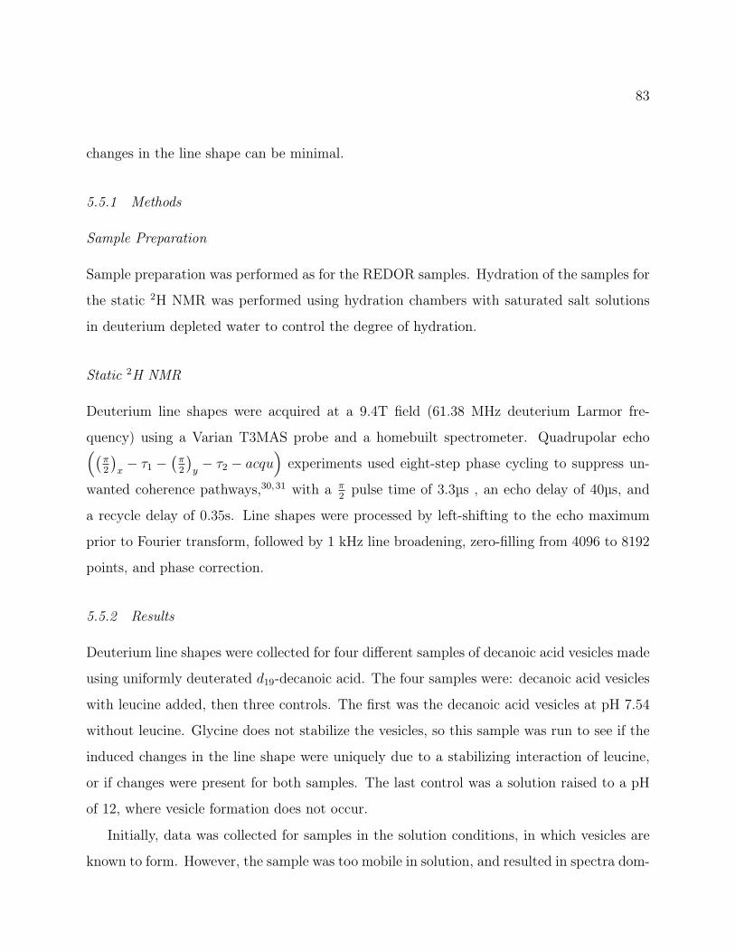
83
changes in the line shape can be minimal.
5.5.1 Methods
Sample Preparation
Sample preparation was performed as for the REDOR samples. Hydration of the samples for
the static 2H NMR was performed using hydration chambers with saturated salt solutions
in deuterium depleted water to control the degree of hydration.
Static 2H NMR
Deuterium line shapes were acquired at a 9.4T field (61.38 MHz deuterium Larmor fre-
quency) using a Varian T3MAS probe and a homebuilt spectrometer. Quadrupolar echo((π2
)x− τ1 −
(π2
)y− τ2 − acqu
)experiments used eight-step phase cycling to suppress un-
wanted coherence pathways,30,31 with a π2pulse time of 3.3µs , an echo delay of 40µs, and
a recycle delay of 0.35s. Line shapes were processed by left-shifting to the echo maximum
prior to Fourier transform, followed by 1 kHz line broadening, zero-filling from 4096 to 8192
points, and phase correction.
5.5.2 Results
Deuterium line shapes were collected for four different samples of decanoic acid vesicles made
using uniformly deuterated d19-decanoic acid. The four samples were: decanoic acid vesicles
with leucine added, then three controls. The first was the decanoic acid vesicles at pH 7.54
without leucine. Glycine does not stabilize the vesicles, so this sample was run to see if the
induced changes in the line shape were uniquely due to a stabilizing interaction of leucine,
or if changes were present for both samples. The last control was a solution raised to a pH
of 12, where vesicle formation does not occur.
Initially, data was collected for samples in the solution conditions, in which vesicles are
known to form. However, the sample was too mobile in solution, and resulted in spectra dom-
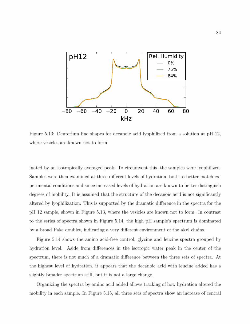
84
Figure 5.13: Deuterium line shapes for decanoic acid lyophilized from a solution at pH 12,
where vesicles are known not to form.
inated by an isotropically averaged peak. To circumvent this, the samples were lyophilized.
Samples were then examined at three different levels of hydration, both to better match ex-
perimental conditions and since increased levels of hydration are known to better distinguish
degrees of mobility. It is assumed that the structure of the decanoic acid is not significantly
altered by lyophilization. This is supported by the dramatic difference in the spectra for the
pH 12 sample, shown in Figure 5.13, where the vesicles are known not to form. In contrast
to the series of spectra shown in Figure 5.14, the high pH sample’s spectrum is dominated
by a broad Pake doublet, indicating a very different environment of the akyl chains.
Figure 5.14 shows the amino acid-free control, glycine and leucine spectra grouped by
hydration level. Aside from differences in the isotropic water peak in the center of the
spectrum, there is not much of a dramatic difference between the three sets of spectra. At
the highest level of hydration, it appears that the decanoic acid with leucine added has a
slightly broader spectrum still, but it is not a large change.
Organizing the spectra by amino acid added allows tracking of how hydration altered the
mobility in each sample. In Figure 5.15, all three sets of spectra show an increase of central

85
Figure 5.14: Deuterium line shapes of d19−decanoic acid with no amino acid, leucine and
glycine added; organized by hydration level. Percent hydration refers to the relative humidity
of the hydration chamber used for sample hydration. All samples were titrated to a pH of
7.55.
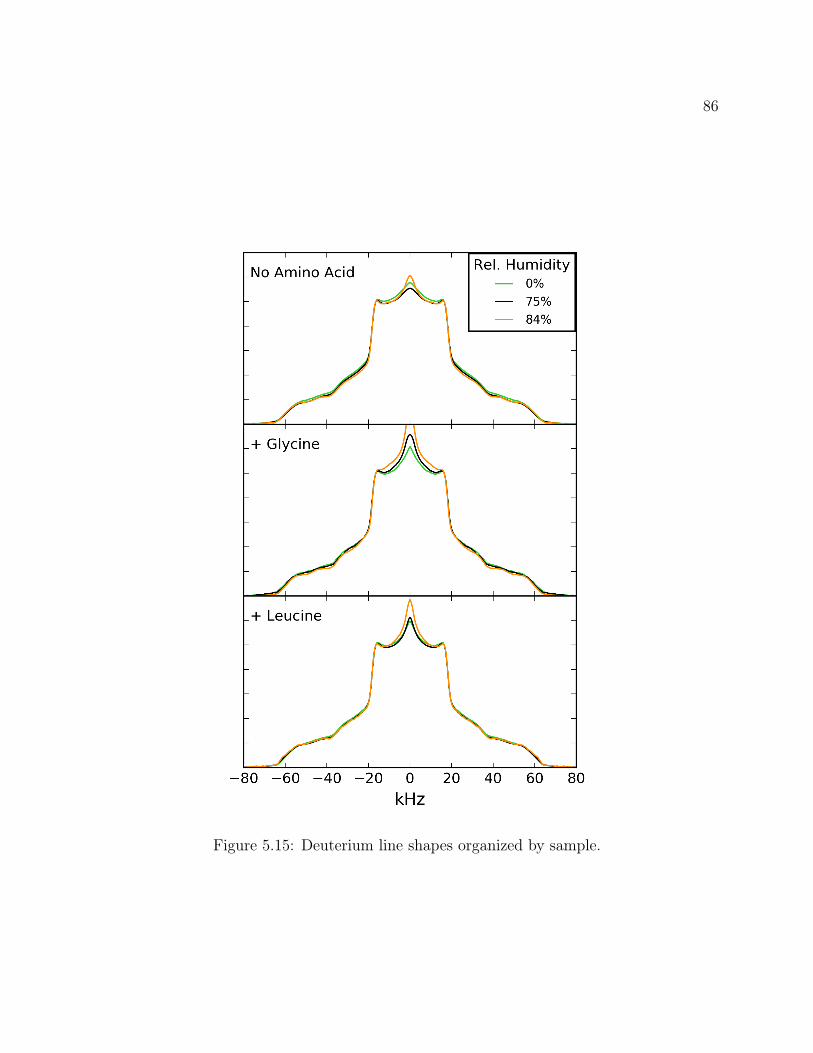
86
Figure 5.15: Deuterium line shapes organized by sample.
87
intensity with increased hydration, but this is simply contribution from residual HDO in the
deuterium depleted water used in the hydration process. Examining the shoulder regions
of these spectra, hydration seems to slightly narrow the line shape for the amino acid-free
and glycine added control samples, while no change is observed for the leucine sample. This
trend is by no means conclusive, due to the minor nature of the line shape changes. The lack
of a significant difference means that no association is shown from this data. As previously
stated, this does not bar the possibility of an associative effect since the fatty acid packing is
looser and more easily interrupted than phospholipids, which is why the REDOR technique
was employed.
88
BIBLIOGRAPHY
[1] N Kröger, R Deutzmann, and M Sumper. Polycationic peptides from diatom biosilicathat direct silica nanosphere formation. Science, 286(5442):1129–1132, Nov 1999.
[2] N Kröger, R Deutzmann, C Bergsdorf, and M Sumper. Species-specific polyaminesfrom diatoms control silica morphology. Proc Natl Acad Sci U S A, 97(26):14133–14138, Dec 2000.
[3] Pascal Lopez, Clementine Gautier, Jacques Livage, and Thibaud Coradin. MimickingBiogenic Silica Nanostructures Formation. Current Nanoscience, 1(1):73–83, Jan 2005.
[4] Francisco Rodríguez, Diana D Glawe, Rajesh R Naik, Kevin P Hallinan, and Morley OStone. Study of the chemical and physical influences upon in vitro peptide-mediatedsilica formation. Biomacromolecules, 5(2):261–265, Mar-Apr 2004.
[5] Marc R. Knecht and David W. Wright. Functional analysis of the biomimetic silica pre-cipitating activity of the R5 peptide from Cylindrotheca fusiformis. Chem. Commun.,pages 3038–3039, 2003.
[6] David J. Belton, Siddharth V. Patwardhan, and Carole C. Perry. Spermine, spermidineand their analogues generate tailored silicas. J. Mater. Chem., 15:4629–4638, 2005.
[7] Nils Kröger, Sonja Lorenz, Eike Brunner, and Manfred Sumper. Self-assembly ofhighly phosphorylated silaffins and their function in biosilica morphogenesis. Science,298(5593):584–586, Oct 2002.
[8] Manfred Sumper, Sonja Lorenz, and Eike Brunner. Biomimetic control of size in thepolyamine-directed formation of silica nanospheres. Angewandte Chemie InternationalEdition, 42(42):5192–5195, 2003.
[9] Manfred Sumper and Nils Kröger. Silica formation in diatoms: the function of long-chain polyamines and silaffins. J. Mater. Chem., 14:2059–2065, 2004.
[10] Igor Pamirsky and Kirill Golokhvast. Silaffins of Diatoms: From Applied Biotechnologyto Biomedicine. Marine Drugs, 11(9):3155–3167, Aug 2013.

89
[11] Ariel C. Zane, Christian Michelet, Adrienne Roehrich, Prashant S. Emani, and Gary P.Drobny. Silica Morphogenesis by Lysine-Leucine Peptides with Hydrophobic Periodic-ity. Langmuir, 30(24):7152–7161, Jun 2014.
[12] Ariel C. Zane. Solid State NMR Characterization of Biosilicification Peptides. PhDthesis, University of Washington, 2013.
[13] Adrienne Roehrich and Gary Drobny. Solid-State NMR Studies of BiomineralizationPeptides and Proteins. Accounts of Chemical Research, 46(9):2136–2144, Sep 2013.
[14] Carolin C. Lechner and Christian F. W. Becker. A sequence-function analysis of thesilica precipitating silaffin R5 peptide. Journal of Peptide Science, 20(2):152–158, 2014.
[15] W. F. DeGrado and J. D. Lear. Induction of Peptide Conformation at Apolar Wa-ter Interfaces. 1. A Study with Model Peptides of Defined Hydrophobic Periodicity.Journal of the American Chemical Society, 107(25):7684–7689, 1985.
[16] W F DeGrado, Z RWasserman, and J D Lear. Protein Design, A Minimalist Approach.Science, 243(4891):622–628, Feb 1989.
[17] P. V. Bower, E. A. Louie, J. R. Long, P. S. Stayton, and G. P. Drobny. Solid-StateNMR Structural Studies of Peptides Immobilized on Gold Nanoparticles. Langmuir,21(7):3002–3007, 2005. PMID: 15779977.
[18] Nicholas F. Breen, Tobias Weidner, Kun Li, David G. Castner, and Gary P. Drobny. ASolid-State Deuterium NMR and Sum-Frequency Generation Study of the Side-ChainDynamics of Peptides Adsorbed onto Surfaces. Journal of the American ChemicalSociety, 131(40):14148–14149, 2009.
[19] Nicholas F. Breen, Kun Li, Gregory L. Olsen, and Gary P. Drobny. DeuteriumMagic Angle Spinning NMR Used To Study the Dynamics of Peptides Adsorbed ontoPolystyrene and Functionalized Polystyrene Surfaces. The Journal of Physical Chem-istry B, 115(30):9452–9460, 2011. PMID: 21650191.
[20] Joanna R. Long, Nathan Oyler, Gary P. Drobny, and Patrick S. Stayton. Assembly ofα-helical Peptide Coatings on Hydrophobic Surfaces. Journal of the American ChemicalSociety, 124(22):6297–6303, 2002. PMID: 12033857.
[21] Tobias Weidner, Nicholas F. Breen, Kun Li, Gary P. Drobny, and David G. Castner.Sum frequency generation and solid-state NMR study of the structure, orientation,and dynamics of polystyrene-adsorbed peptides. Proceedings of the National Academyof Sciences, 107(30):13288–13293, 2010.
90
[22] Ozzy Mermut, Diana C. Phillips, Roger L. York, Keith R. McCrea, Robert S. Ward,and Gabor A. Somorjai. In Situ Adsorption Studies of a 14-Amino Acid Leucine-LysinePeptide onto Hydrophobic Polystyrene and Hydrophilic Silica Surfaces Using QuartzCrystal Microbalance, Atomic Force Microscopy, and Sum Frequency Generation Vi-brational Spectroscopy. Journal of the American Chemical Society, 128(11):3598–3607,2006. PMID: 16536533.
[23] Diana C. Phillips, Roger L. York, Ozzy Mermut, Keith R. McCrea, Robert S. Ward,and Gabor A. Somorjai. Side Chain, Chain Length, and Sequence Effects on Am-phiphilic Peptide Adsorption at Hydrophobic and Hydrophilic Surfaces Studied bySum-Frequency Generation Vibrational Spectroscopy and Quartz Crystal Microbal-ance. The Journal of Physical Chemistry C, 111(1):255–261, 2007.
[24] Roger L. York, William K. Browne, Phillip L. Geissler, and Gabor A. Somorjai. Pep-tides Adsorbed on Hydrophobic Surfaces—A Sum Frequency Generation VibrationalSpectroscopy and Modeling Study. Israel Journal of Chemistry, 47(1):51–58, 2007.
[25] Eric F Pettersen, Thomas D Goddard, Conrad C Huang, Gregory S Couch, Daniel MGreenblatt, Elaine C Meng, and Thomas E Ferrin. UCSF Chimera–a visualizationsystem for exploratory research and analysis. J Comput Chem, 25(13):1605–1612, Oct2004.
[26] Yang Shen and Ad Bax. Protein backbone and sidechain torsion angles predicted fromNMR chemical shifts using artificial neural networks. Journal of Biomolecular NMR,56(3):227–241, 2013.
[27] Joe E. Baio, Ariel Zane, Vance Jaeger, Adrienne M. Roehrich, Helmut Lutz, JimPfaendtner, Gary P. Drobny, and Tobias Weidner. Diatom Mimics: Directing theFormation of Biosilica Nanoparticles by Controlled Folding of Lysine-Leucine Pep-tides. Journal of the American Chemical Society, 136(43):15134–15137, 2014. PMID:25285787.
[28] Todd M. Alam and Gary P. Drobny. Solid-state NMR studies of DNA structure anddynamics. Chemical Reviews, 91(7):1545–1590, 1991.
[29] J. H. Davis. Deuterium nuclear magnetic resonance spectroscopy in partially orderedsystems, chapter 3. Elsevier, 1991.
[30] Melinda J. Duer, editor. Solid-State NMR Spectroscopy: principles and applications.Blackwell Science Ltd, 2002.
91
[31] Robert Tycko, editor. Nuclear Magnetic Resonance Probes of Molecular Dynamics.Kluwer Academic Publishers, 1994.
[32] H. W Spiess and H Sillescu. Solid echoes in the slow-motion region. Journal of MagneticResonance (1969), 42(3):381–389, Mar 1981.
[33] Jørgen H. Kristensen, Henrik Bildsøe, Hans J. Jakobsen, and Niels Chr. Nielsen. The-ory and simulations of molecular dynamics in 2H MAS NMR. Journal of MagneticResonance, 100(2):437 – 443, 1992.
[34] Robert L. Vold and Gina L. Hoatson. Effects of jump dynamics on solid state nu-clear magnetic resonance line shapes and spin relaxation times. Journal of MagneticResonance, 198(1):57 – 72, 2009.
[35] R. J. Wittebort, E. T. Olejniczak, and R. G. Griffin. Analysis of deuterium nuclearmagnetic resonance line shapes in anisotropic media. The Journal of Chemical Physics,86(10):5411–5420, 1987.
[36] M.J. Duer and M.H. Levitt. Time-domain calculation of chemical exchange effects inthe NMR spectra of rotating solids. Solid State Nuclear Magnetic Resonance, 1(4):211–215, Nov 1992.
[37] Dr. Phillip M. Feldman. Eight Advantages of Python Over Matlab,http://phillipmfeldman.org/Python/Advantages_of_Python_Over_Matlab.html.
[38] Hoyt Koepke. 10 Reasons Python Rocks for Research (And a Few Reasons it Doesn’t),http://www.stat.washington.edu/~hoytak/blog/whypython.html.
[39] Asher Schmidt, Steven O. Smith, Daniel P. Raleigh, James E. Roberts, Robert G.Griffin, and Shimon Vega. Chemical exchange effects in the NMR spectra of rotatingsolids. The Journal of Chemical Physics, 85(8):4248, 1986.
[40] O Weintraub and S Vega. Dynamic 2H nuclear magnetic resonance of rotating solids.Solid State Nuclear Magnetic Resonance, 4(6):341–351, Aug 1995.
[41] J H Kristensen, G L Hoatson, and Robert L Vold. Effects of restricted rotationaldiffusion on 2H magic angle spinning nuclear magnetic resonance spectra. The Journalof Chemical Physics, 110(9):4533, 1999.
[42] Michael J. Thrippleton, Marica Cutajar, and Stephen Wimperis. Magic angle spinning(MAS) NMR linewidths in the presence of solid-state dynamics. Chemical PhysicsLetters, 452(4-6):233–238, Feb 2008.

92
[43] Kun Li. Use Deuterium Solid State NMR Simulations to Study Dynamics of PeptidesAdsorbed onto Inorganic Surfaces. PhD thesis, University of Washington, 2012.
[44] Vera B. Cheng, Henry H. Suzukawa, and MaxWolfsberg. Investigations of a nonrandomnumerical method for multidimensional integration. The Journal of Chemical Physics,59(8):3992–3999, 1973.
[45] Harold Conroy. Molecular Schrödinger Equation. VIII. A New Method for the Eval-uation of Multidimensional Integrals. The Journal of Chemical Physics, 47(12):5307–5318, 1967.
[46] S. K. Zaremba. Good lattice points, discrepancy, and numerical integration. Annali diMatematica Pura ed Applicata, 73(1):293–317, Dec 1966.
[47] Malcolm Levitt. Orientations for Powder Averaging,http://www.southampton.ac.uk/~mhl/resources/Orientations/index.html.
[48] Wei Liu, Evan Crocker, Stefan N Constantinescu, and Steven O Smith. Helix packingand orientation in the transmembrane dimer of gp55-P of the spleen focus formingvirus. Biophys J, 89(2):1194–1202, Aug 2005.
[49] Kathleen P. Howard, Wei Liu, Evan Crocker, Vikas Nanda, James Lear, William F.Degrado, and Steven O. Smith. Rotational orientation of monomers within a designedhomo-oligomer transmembrane helical bundle. Protein Science, 14(4):1019–1024, 2005.
[50] Weiwen Ying, Scott E. Irvine, Richard A. Beekman, David J. Siminovitch, andSteven O. Smith. Deuterium NMR Reveals Helix Packing Interactions in Phospho-lamban. Journal of the American Chemical Society, 122(45):11125–11128, 2000.
[51] Joanna R. Long, Frank D. Mills, Omjoy K. Ganesh, Vijay C. Antharam, andR. Suzanne Farver. Partitioning, dynamics, and orientation of lung surfactant peptideKL4 in phospholipid bilayers. Biochimica et Biophysica Acta (BBA) - Biomem-branes, 1798(2):216 – 222, 2010. Membrane Protein Dynamics by NMR: Correlationof Structure and Function.
[52] Eva Meirovitch, Zhichun Liang, and Jack H Freed. Protein dynamics in the solidstate from 2H NMR line shape analysis: a consistent perspective. J Phys Chem B,119(7):2857–2868, Feb 2015.
[53] Eva Meirovitch, Zhichun Liang, and Jack H Freed. Protein Dynamics in the Solid Statefrom 2H NMR Line Shape Analysis. II. MOMD Applied to C–D and C–CD3 Probes.The Journal of Physical Chemistry B, 119(44):14022–14032, 2015.
93
[54] L W Jelinski, C E Sullivan, L S Batchelder, and D A Torchia. Deuterium nuclear mag-netic resonance of specifically labeled native collagen. investigation of protein moleculardynamics using the quadrupolar echo technique. Biophys J, 32(1):515–529, Oct 1980.
[55] L S Batchelder, C E Sullivan, L W Jelinski, and D A Torchia. Characterization ofleucine side-chain reorientation in collagen-fibrils by solid-state 2H NMR. Proceedingsof the National Academy of Sciences, 79(2):386–389, 1982.
[56] Liliya Vugmeyster, Dmitry Ostrovsky, Joseph J. Ford, Sarah D. Burton, Andrew S.Lipton, Gina L. Hoatson, and Robert L. Vold. Probing the Dynamics of a ProteinHydrophobic Core by Deuteron Solid-State Nuclear Magnetic Resonance Spectroscopy.Journal of the American Chemical Society, 131(38):13651–13658, 2009.
[57] Liliya Vugmeyster, Dmitry Ostrovsky, Mark Moses, Joseph J. Ford, Andrew S. Lipton,Gina L. Hoatson, and Robert L. Vold. Comparative Dynamics of Leucine MethylGroups in FMOC-Leucine and in a Protein Hydrophobic Core Probed by Solid-StateDeuteron Nuclear Magnetic Resonance over 7-324 K Temperature Range. The Journalof Physical Chemistry B, 114(48):15799–15807, 2010.
[58] Liliya Vugmeyster, Dmitry Ostrovsky, Joseph J. Ford, and Andrew S. Lipton. Freezingof Dynamics of a Methyl Group in a Protein Hydrophobic Core at Cryogenic Temper-atures by Deuteron NMR Spectroscopy. Journal of the American Chemical Society,132(12):4038–4039, 2010.
[59] Liliya Vugmeyster, Dmitry Ostrovsky, Anastasia Khadjinova, Jeremy Ellden, Gina L.Hoatson, and Robert L. Vold. Slow Motions in the Hydrophobic Core of Chicken VillinHeadpiece Subdomain and Their Contributions to Configurational Entropy and HeatCapacity from Solid-State Deuteron NMR Measurements. Biochemistry, 50(49):10637–10646, 2011.
[60] Liliya Vugmeyster, Dmitry Ostrovsky, Kirsten Penland, Gina L. Hoatson, andRobert L. Vold. Glassy Dynamics of Protein Methyl Groups Revealed by DeuteronNMR. The Journal of Physical Chemistry B, 117(4):1051–1061, 2013.
[61] Liliya Vugmeyster, Tien Do, Dmitry Ostrovsky, and Riqianq Fu. Effect of subdomaininteractions on methyl group dynamics in the hydrophobic core of villin headpieceprotein. Protein Sci, 23(2):145–156, Feb 2014.
[62] Shadi Abu-Baker, Jun-Xia Lu, Shidong Chu, Clarke C Brinn, Christopher A Makaroff,and Gary A Lorigan. Side chain and backbone dynamics of phospholamban in phos-pholipid bilayers utilizing 2H and 15N solid-state NMR spectroscopy. Biochemistry,46(42):11695–11706, 2007.
94
[63] Shidong Chu, Aaron T. Coey, and Gary A. Lorigan. Solid-state 2H and 15N NMRstudies of side-chain and backbone dynamics of phospholamban in lipid bilayers: In-vestigation of the N27A mutation. Biochimica et Biophysica Acta (BBA) - Biomem-branes, 1798(2):210 – 215, 2010. Membrane Protein Dynamics by NMR: Correlationof Structure and Function.
[64] Ethan S. Karp, Elvis K. Tiburu, Shadi Abu-Baker, and Gary A. Lorigan. The struc-tural properties of the transmembrane segment of the integral membrane protein phos-pholamban utilizing 13C CPMAS, 2H, and REDOR solid-state NMR spectroscopy.Biochimica et Biophysica Acta (BBA) - Biomembranes, 1758(6):772 – 780, 2006.
[65] Elvis K Tiburu, Ethan S Karp, Paresh C Dave, Krishnan Damodaran, and Gary ALorigan. Investigating the dynamic properties of the transmembrane segment of phos-pholamban incorporated into phospholipid bilayers utilizing 2H and 15N solid-stateNMR spectroscopy. Biochemistry, 43(44):13899–13909, 2004.
[66] Abil E. Aliev and Kenneth D. M. Harris. 2H NMR lineshape analysis using automatedfitting procedures based on local and quasi-global optimization techniques. MagneticResonance in Chemistry, 36(11):855–868, 1998.
[67] Kun Li, Prashant S. Emani, Jason Ash, Michael Groves, and Gary P. Drobny. A Studyof Phenylalanine Side-Chain Dynamics in Surface-Adsorbed Peptides Using Solid-StateDeuterium NMR and Rotamer Library Statistics. Journal of the American ChemicalSociety, 136(32):11402–11411, 2014. PMID: 25054469.
[68] Emile Aarts, Jan Korst, and Wil Michiels. Simulated Annealing. In Search Method-ologies, number 1999, pages 187–210. Springer US, Boston, MA, 2005.
[69] L. Ingber. Simulated annealing: Practice versus theory. Mathematical and ComputerModelling, 18(11):29–57, Dec 1993.
[70] Gunter Dueck and Tobias Scheuer. Threshold accepting: A general purpose optimiza-tion algorithm appearing superior to simulated annealing. Journal of ComputationalPhysics, 90(1):161–175, Sep 1990.
[71] Tejas P Patalia and G R Kulkarni. Comparative Analysis of Threshold AcceptanceAlgorithm, Simulated Annealing Algorithm and Genetic Algorithm for Function Opti-mization. Global Journal of researches in Engineering Numerical Methods, 12(1):23–27,2012.
[72] Kathleen Wood, François-Xavier Gallat, Renee Otten, Auke J. van Heel, MathildeLethier, Lambert van Eijck, Martine Moulin, Michael Haertlein, Martin Weik, and

95
Frans A. A. Mulder. Protein surface and core dynamics show concerted hydration-dependent activation. Angewandte Chemie International Edition, 52(2):665–668, 2013.
[73] Maggy Hologne and Jérôme Hirschinger. Molecular dynamics as studied by static-powder and magic-angle spinning 2H NMR. Solid State Nuclear Magnetic Resonance,26(1):1–10, Aug 2004.
[74] Maxim V. Shapovalov and Jr. Dunbrack, Roland L. A smoothed backbone-dependentrotamer library for proteins derived from adaptive kernel density estimates and regres-sions. Structure, 19(6):844–858, June 2011.
[75] M A Keniry, A Kintanar, R L Smith, H S Gutowsky, and E Oldfield. Nuclear magneticresonance studies of amino acids and proteins. deuterium nuclear magnetic resonancerelaxation of deuteriomethyl-labeled amino acids in crystals and in halobacterium halo-bium and escherichia coli cell membranes. Biochemistry, 23(2):288–298, Jan 1984.
[76] D. Flemming Hansen, Philipp Neudecker, Pramodh Vallurupalli, Frans A. A. Mulder,and Lewis E. Kay. Determination of Leu Side-Chain Conformations in Excited ProteinStates by NMR Relaxation Dispersion. Journal of the American Chemical Society,132(1):42–43, 2010. PMID: 20000605.
[77] D. Flemming Hansen, Philipp Neudecker, and Lewis E. Kay. Determination ofIsoleucine Side-Chain Conformations in Ground and Excited States of Proteins fromChemical Shifts. Journal of the American Chemical Society, 132(22):7589–7591, 2010.PMID: 20465253.
[78] Carolin C Lechner and Christian F W Becker. Modified silaffin R5 peptides enableencapsulation and release of cargo molecules from biomimetic silica particles. BioorgMed Chem, 21(12):3533–3541, Jun 2013.
[79] Céline Auger, Anne Lesage, Stefano Caldarelli, Paul Hodgkinson, and Lyndon Emsley.Deuterium-Carbon NMR Correlation Spectroscopy in Oriented Materials. Journal ofthe American Chemical Society, 119(49):12000–12001, Dec 1997.
[80] Xiangyan Shi, Jeffery L Yarger, and Gregory P Holland. Elucidating proline dynamicsin spider dragline silk fibre using 2H-13C HETCOR MAS NMR. Chemical communi-cations (Cambridge, England), pages 13–16, 2014.
[81] Xiangyan Shi, Gregory P. Holland, and Jeffery L. Yarger. Molecular Dynamics of SpiderDragline Silk Fiber Investigated by 2H MAS NMR. Biomacromolecules, 16(3):852–859,2015.
96
[82] Xiangyan Shi, Jeffery L. Yarger, and Gregory P. Holland. 2H–13C HETCOR MASNMR for indirect detection of 2H quadrupole patterns and spin–lattice relaxation rates.Journal of Magnetic Resonance, 226:1–12, Jan 2013.
[83] K. Torii and Y. Iitaka. The crystal structure of L-isoleucine. Acta CrystallographicaSection B Structural Crystallography and Crystal Chemistry, 27(11):2237–2246, 1971.
[84] A. Lesage, C. Auger, S. Caldarelli, and L. Emsley. Determination of through-bondcarbon-carbon connectivities in solid-state NMR using the INADEQUATE experiment.Journal of the American Chemical Society, 119(33):7867–7868, 1997.
[85] Alexander D Scouras and Valerie Daggett. The dynameomics rotamer library: Aminoacid side chain conformations and dynamics from comprehensive molecular dynamicssimulations in water. Protein Science : A Publication of the Protein Society, 20(2):341–352, 02 2011.
[86] R. Dawkins. The Blind Watchmaker, page 1. Number 1986. W.W. Norton and Com-pany, New York, USA, 1986.
[87] Moshe Gordon, Roy A. Black, Matthew C. Blosser, and Sarah L. Keller. Aminoacids and peptides stabilize fatty acid membranes against salt-induced flocculation.Biophysical Journal, 108(2):542a, 2016/04/12.
[88] W R Hargreaves, S J Mulvihill, and D W Deamer. Synthesis of phospholipids andmembranes in prebiotic conditions. Nature, 266(5597):78–80, Mar 1977.
[89] A D Bangham. Membrane models with phospholipids. Prog Biophys Mol Biol, 18:29–95, 1968.
[90] Pierre-Alain Monnard and David W. Deamer. Membrane self-assembly processes:Steps toward the first cellular life. The Anatomical Record, 268(3):196–207, 2002.
[91] Kenichi Morigaki, Peter Walde, Misni Misran, and Brian H Robinson. Thermody-namic and kinetic stability. Properties of micelles and vesicles formed by the decanoicacid/decanoate system. Colloids and Surfaces A: Physicochemical and EngineeringAspects, 213(1):37 – 44, 2003.
[92] Hiroshi Naraoka, Akira Shimoyama, and Kaoru Harada. Molecular Distribution ofMonocarboxylic Acids in Asuka Carbonaceous Chondrites from Antarctica. Origins oflife and evolution of the biosphere, 29(2):187–201, March 1999.
97
[93] Roy A. Black, Matthew C. Blosser, Benjamin L. Stottrup, Ravi Tavakley, David W.Deamer, and Sarah L. Keller. Nucleobases bind to and stabilize aggregates of a prebioticamphiphile, providing a viable mechanism for the emergence of protocells. Proceedingsof the National Academy of Sciences, 110(33):13272–13276, 2013.
[94] Dick Sandström, Mei Hong, and Klaus Schmidt-Rohr. Identification and mobility ofdeuterated residues in peptides and proteins by 2H-13C solid-state NMR. ChemicalPhysics Letters, 300(1-2):213–220, Jan 1999.
[95] Terry Gullion, Raghuvansh Kishore, and Tetsuo Asakura. Determining Dihedral Anglesand Local Structure in Silk Peptide by 13C - 2H REDOR. Journal of the AmericanChemical Society, 125(25):7510–7511, Jun 2003.
[96] Lihui Jia, Shuang Liang, Kelly Sackett, Li Xie, Ujjayini Ghosh, and David P. We-liky. REDOR solid-state NMR as a probe of the membrane locations of membrane-associated peptides and proteins. Journal of Magnetic Resonance, 253:154–165, Apr2015.
[97] Li Xie, Ujjayini Ghosh, Scott D. Schmick, and David P. Weliky. Residue-specificmembrane location of peptides and proteins using specifically and extensively deuter-ated lipids and 13C–2H rotational-echo double-resonance solid-state NMR. Journal ofBiomolecular NMR, 55(1):11–17, Jan 2013.
[98] Suman A. Luthra, Marcel Utz, Eric M. Gorman, Michael J. Pikal, Eric J. Munson,and Joseph W. Lubach. Carbon–Deuterium Rotational-Echo Double-Resonance NMRSpectroscopy of Lyophilized Aspartame Formulations. Journal of Pharmaceutical Sci-ences, 101(1):283–290, January 2012.
[99] Thomas Bräuniger, Philip Wormald, and Paul Hodgkinson. Improved Proton Decou-pling in NMR Spectroscopy of Crystalline Solids Using the Spinal-64 Sequence, pages69–74. Springer Vienna, Vienna, 2003.
[100] P.S. Belton, A.M. Gil, and S.F. Tanner. On the 13C spectra of leucine. Solid StateNuclear Magnetic Resonance, 1(2):67–71, Jun 1992.
[101] Eleri Hughes, Jonathan C. Clayton, and David a. Middleton. Probing the OligomericState of Phospholamban Variants in Phospholipid Bilayers from Solid-State NMRMea-surements of Rotational Diffusion Rates. Biochemistry, 44(10):4055–4066, Mar 2005.
[102] Byungsu Kwon, Alan J. Waring, and Mei Hong. A 2H Solid-State NMR Study of LipidClustering by Cationic Antimicrobial and Cell-Penetrating Peptides in Model BacterialMembranes. Biophysical Journal, 105(10):2333–2342, Nov 2013.
98
[103] Judith A. Barry and Klaus Gawrisch. Direct NMR Evidence for Ethanol Binding tothe Lipid-Water Interface of Phospholipid Bilayers. Biochemistry, 33(26):8082–8088,Jul 1994.
[104] J.H. Davis, K.R. Jeffrey, M. Bloom, M.I. Valic, and T.P. Higgs. Quadrupolar echodeuteron magnetic resonance spectroscopy in ordered hydrocarbon chains. ChemicalPhysics Letters, 42(2):390 – 394, 1976.
[105] M Lafleur, B Fine, E Sternin, P R Cullis, and M Bloom. Smoothed orientationalorder profile of lipid bilayers by 2H-nuclear magnetic resonance. Biophysical Journal,56(5):1037–1041, 11 1989.
[106] Liliya Vugmeyster, Dmitry Ostrovsky, Toni Villafranca, Janelle Sharp, Wei Xu, An-drew S Lipton, Gina L Hoatson, and Robert L Vold. Dynamics of HydrophobicCore Phenylalanine Residues Probed by Solid-State Deuteron NMR. J Phys ChemB, 119(47):14892–14904, Nov 2015.
[107] S L Miller and H C Urey. Organic compound synthesis on the primitive earth. Science,130(3370):245–251, Jul 1959.
[108] Naomi H.M. Hogg, Paul J.T. Boulton, Vadim E. Zorin, Robin K. Harris, and PaulHodgkinson. Use of rotary echoes in magic-angle spinning NMR for the quantitativestudy of molecular dynamics. Chemical Physics Letters, 475(1-3):58–63, Jun 2009.
[109] Asher Schmidt and Shimon Vega. NMR line shape analysis for two-site exchange inrotating solids. The Journal of Chemical Physics, 87(12):6895, 1987.

99
Appendix A
WHERE TO FIND THE FILES
A.1 Setup
If you have minimal coding experience or are moving to Python from MATLAB, the eas-
iest way to install and get start is to download a program like Spyder, available here:
https://github.com/spyder-ide/spyder. Spyder is the Scientific PYthon Development
EnviRonment, and it can be a good way to get started. I ultimately prefer to install Python
separately, I feel that it runs more smoothly. If you’re interested in that, continue reading.
A.1.1 Installing Python on a Mac
• Install XCode from https://developer.apple.com/xcode/
• In the Terminal, run the following line:
$ xcode -select --install
• install Homebrew using:
1 /usr/bin/ruby -e "$(curl -fsSL https :// raw.githubusercontent.com/Homebrew/install/
master/install)"
brew install python3
pip3 install ipython
pip3 install numpy
pip3 install scipy
pip3 install nose
pip3 install matplotlib
100
A.1.2 Package, (version used)
• Python (3.4.3)
• iPython (4.1.2)
• numpy (1.11.0)
• scipy (0.17.0)
• nose (1.3.7)
• matplotlib (1.5.1)
To edit files, you can use any text editor. I prefer to use TextWrangler. It is free through
the App Store, and will do syntax highlighting, that is, it will change the color of key words
in the coding language you are using, as well as change colors of comments to distinguish
them from the code itself.
A.1.3 First Steps
You should now have a working version of Python installed! If you downloaded Spyder,
launch the interface and go to town!
If you want to mess around with the basics of python in the Terminal, you can launch a
session by typing:
$ ipython
If you want to run a script you have written (see next section for examples), navigate
to that file in the Terminal. (Using the cd command to change directories) For example, if
your script is called file.py in Folder:
$ cd Folder
$ ipython file.py

101
If ssh-ing into a Linux system, jobs can be submitted as above. To avoid stopping jobs upon
logout, jobs can be submitted as follows:
$ nohup ipython file.py &
$ exit
Any printed text output will be stored in a file called nohup.out.
A.2 Basic Input Files
A.2.1 Quadrupolar Echo Input
Dropbox\HEFCode\paramQE.py
1 """
2 import modules , functions from other files
3 """
4 import numpy as np #python package for arrays
5 import matplotlib.pyplot as plt #for plotting data
6 from oneSiteMatrix import chi2euler , chi2eulerMethyl #only needed in special cases
7 from simQE import runSim as run #import runSim method from the appropriate simulator
8
9 """
10 paramfileQE
11 2 site jump with Explicit Methyl Rotation , 6k tiles
12 """
13
14 """
15 Basic Parameters
16 """
17 param = #Initialize a dictionary for holding relevant parameters
18 param['dwell ']=.8 #dwell time in micro seconds (10^ -6)
19 param['taudelay ']=40. #delay between pi pulses in microseconds
20 param['ntiles ']=6000 #number of tiles used to integrate powder pattern
21 param['nfidpts ']=512*2 #number of FID points to calculate
22
23 """
24 Set of special flags for handling of special cases
25 """
26 param['chionly?']=False
27 param['all_contributions '] = True
28 param['chimethyl?']=False
102
29 param['chi?']= True
30
31 """
32 Site definitions
33 """
34 """
35 param['cq ']: QCC in kHz
36 param['anglemats ']: Orientation frames in the form: [[ frame1],[frame2 ],...], with [frame] =
[[ angle1],[angle2 ] ,...]. angles are Euler angles as described in Chapter 2, in degrees.
Note that for a single site you still need all the brackets , [[frame ]]=[[[ angle ]]]
37 param['ratemats ']: Site connectivity and rates for each frame , in the form [[k1,Connectivity
] ,...]. Preset connectivities are described in Appendix B, see oneRateMatrix
38 param['sitepops ']: Populations for each site , note that if you have a repeating list you can
do as follows: [1. ,]*6
39 """
40 state = [10.8, 8.3, 411958.0398583684 , 48.8, 156.3, 66.37173042089874 , 4.0,
2.778452529613264 , 15.0, 2.7584315260835806 , 8.80509919854084e-07]
41
42 param['cq_delta ']=state [3]
43 param['cq_gamma ']=state [4]
44 param['%gamma']=.15
45 param['eta']=0.
46 param['chiangles '] = [[-68.9, -88.9, -96.3, -161.2, -166.5, -178.8] ,[172.7 , -61.1, 40.9,
171.9, -76.9, 60.6]]
47
48 param['anglemats ']=[ chi2euler(param['chiangles '],param['all_contributions '])]
49 param['ratemats ']=[[( state [0], state[1], state [2]), 'Chi6']]
50
51 param['sitepops ']=[ state[5], state[7],state [8],state[9], state [10], state [6]]
52
53 """
54 Parameters for processing the FID before FT
55 """
56 param['llb']=1 #Lorentzian line broadening in kHz
57 param['glb']=0 #Gaussian line broadening in kHz
58 param['zerofill ']=5 #zero filling: total number of spectral points = nFID *2**zf
59
60 param = run(param) #runs the simulation , for details see Appendix B
61
62 """
63 Manipulation of data , for example plotting the spectrum
64 """

103
65 freq_axis = param['freq_axis ']
66 gSpec , mSpec = param['specg '].real , param['specm '].real
67
68 plt.xlim (-60,60)
69 plt.plot(freq_axis ,gSpec -np.amin(gSpec))
70 plt.plot(freq_axis ,mSpec -np.amin(mSpec))
71 plt.show()
72
73 plt.xlim (-60,60)
74 plt.plot(freq_axis ,gSpec+mSpec -np.amin(gSpec+mSpec))
75 plt.show()
Dropbox\HEFCode\paramQE.py
1 """
2 import modules , functions from other files
3 """
4 import numpy as np #python package for arrays
5 import matplotlib.pyplot as plt #for plotting data
6 from oneSiteMatrix import chi2euler , chi2eulerMethyl #only needed in special cases
7 from simQE import runSim as run #import runSim method from the appropriate simulator
8
9 """
10 paramfileQE
11 2 site jump with Explicit Methyl Rotation , 6k tiles
12 """
13
14 """
15 Basic Parameters
16 """
17 param = #Initialize a dictionary for holding relevant parameters
18 param['dwell ']=.8 #dwell time in micro seconds (10^ -6)
19 param['taudelay ']=40. #delay between pi pulses in microseconds
20 param['ntiles ']=6000 #number of tiles used to integrate powder pattern
21 param['nfidpts ']=512*2 #number of FID points to calculate
22
23 """
24 Set of special flags for handling of special cases
25 """
26 param['chionly?']=False
27 param['all_contributions '] = True
28 param['chimethyl?']=False
29 param['chi?']= True

104
30
31 """
32 Site definitions
33 """
34 """
35 param['cq ']: QCC in kHz
36 param['anglemats ']: Orientation frames in the form: [[ frame1],[frame2 ],...], with [frame] =
[[ angle1],[angle2 ] ,...]. angles are Euler angles as described in Chapter 2, in degrees.
Note that for a single site you still need all the brackets , [[frame ]]=[[[ angle ]]]
37 param['ratemats ']: Site connectivity and rates for each frame , in the form [[k1,Connectivity
] ,...]. Preset connectivities are described in Appendix B, see oneRateMatrix
38 param['sitepops ']: Populations for each site , note that if you have a repeating list you can
do as follows: [1. ,]*6
39 """
40 state = [10.8, 8.3, 411958.0398583684 , 48.8, 156.3, 66.37173042089874 , 4.0,
2.778452529613264 , 15.0, 2.7584315260835806 , 8.80509919854084e-07]
41
42 param['cq_delta ']=state [3]
43 param['cq_gamma ']=state [4]
44 param['%gamma']=.15
45 param['eta']=0.
46 param['chiangles '] = [[-68.9, -88.9, -96.3, -161.2, -166.5, -178.8] ,[172.7 , -61.1, 40.9,
171.9, -76.9, 60.6]]
47
48 param['anglemats ']=[ chi2euler(param['chiangles '],param['all_contributions '])]
49 param['ratemats ']=[[( state [0], state[1], state [2]), 'Chi6']]
50
51 param['sitepops ']=[ state[5], state[7],state [8],state[9], state [10], state [6]]
52
53 """
54 Parameters for processing the FID before FT
55 """
56 param['llb']=1 #Lorentzian line broadening in kHz
57 param['glb']=0 #Gaussian line broadening in kHz
58 param['zerofill ']=5 #zero filling: total number of spectral points = nFID *2**zf
59
60 param = run(param) #runs the simulation , for details see Appendix B
61
62 """
63 Manipulation of data , for example plotting the spectrum
64 """
65 freq_axis = param['freq_axis ']

105
66 gSpec , mSpec = param['specg '].real , param['specm '].real
67
68 plt.xlim (-60,60)
69 plt.plot(freq_axis ,gSpec -np.amin(gSpec))
70 plt.plot(freq_axis ,mSpec -np.amin(mSpec))
71 plt.show()
72
73 plt.xlim (-60,60)
74 plt.plot(freq_axis ,gSpec+mSpec -np.amin(gSpec+mSpec))
75 plt.show()
A.2.2 Magic Angle Spinning Input
Dropbox\HEFCode\paramMAS.py
1 import numpy as np
2 import matplotlib.pyplot as plt #for plotting data
3 from simMAS import runSim as run #import runSim method from the appropriate simulator
4
5 """
6 paramfileMAS
7 3x6 site jump with 6000 tiles
8 """
9
10 """
11 Basic Parameters
12 """
13 param = #Initialize a dictionary for holding relevant parameters
14 param['ntiles ']=6000 #number of tiles used to integrate powder pattern
15 param['nfidpts ']=512 #number of FID points to calculate
16
17 """
18 MAS Specific Parameters
19 """
20 param['spinrate ']=4000 #spinning speed in Hz
21 param['rotfrac ']=64 #number of points calculated per rotor period
22 #param['leftshift ']=0 #note , this is now zero because not a QE
23 param['dwell ']=1/( param['spinrate ']*param['rotfrac ']) #dwell is calculated from above
24
25 """
26 Set of special flags for handling of special cases
27 """
106
28 param['chionly?']=False
29 param['chimethyl?']=False
30 param['chi?']= False
31
32 """
33 Site definitions
34 """
35 param['cq']=152.
36 d=5 #using variables to slightly offset angles
37 e=1.4
38 param['anglemats ']=[[[0 ,68 ,0] ,[0 ,68 ,120] ,[0 ,68 ,240]] ,[[0 ,90 ,0] ,[0 ,90 -d,60+e],[0,90-d,120-e
] ,[0 ,90 ,180] ,[0 ,90+d ,240+e],[0,90+d,300-e]]]
39 param['ratemats ']=[[5*10**10 , 'All'] ,[1.5*10**8 ,'Circle ']]
40 param['sitepops ']=[1. ,]*18
41
42 """
43 Parameters for processing the FID before FT
44 """
45 param['llb']=0 #Lorentzian line broadening in kHz
46 param['glb']=0 #Gaussian line broadening in kHz
47 param['zerofill ']=1 #zero filling: total number of spectral points = nFID *2**zf
48
49 param = run(param) #returns param['FID '], param['spec '], param['freq_axis ']
50
51 """
52 Manipulation of data , for example plotting the spectrum
53 """
54 plt.xlim (-80,80)
55 plt.plot(param['freq_axis '],param['spec']/np.amax(param['spec'].real))
56 plt.show() #plt.savefig('mastest.png ', dpi = 300, bbox_inches='tight ') #swap to have
it saved instead
A.2.3 T1IR Input
Dropbox\HEFCode\paramT1.py
1 import numpy as np
2 from simT1IR import runSim as run #import runSim method from the appropriate simulator
3 import matplotlib.pyplot as plt #for plotting data
4 from scipy.optimize import minimize , curve_fit #for fitting t1
5
6 """
107
7 paramfileT1
8 2 site jump with Explicit Methyl Rotation , 2k tiles
9 """
10
11 """
12 Basic Parameters
13 """
14 param = #Initialize a dictionary for holding relevant parameters
15 param['dwell ']=2. #dwell time in micro seconds (10^ -6)
16 param['taudelay ']=30. #delay between pi pulses in microseconds
17 param['ntiles ']=6000 #number of tiles used to integrate powder pattern
18 param['nfidpts ']=256 #number of FID points to calculate
19
20 """
21 Relaxation Specific Parameters
22 """
23 param['w0']=76.753 #this is the strength of the 500MHz
24 param['taulist ']=[.001 ,.01 ,.02 ,.03 ,.05 ,.1 ,.2 ,.4] #in seconds
25
26 """
27 Set of special flags for handling of special cases
28 """
29 param['chionly?']=False
30 param['chimethyl?']=False
31 param['chi?']= False
32
33 """
34 Site definitions
35 """
36 param['cq']=160.
37 param['anglemats ']=[[[0 ,71 ,0] ,[0 ,71 ,120] ,[0 ,71 ,240]] ,[[0 ,53 ,0] ,[0 ,53 ,180]]]
38 param['ratemats ']=[[5*10**9 , 'Circle '],[2000,'All']]
39 param['sitepops ']=[1. ,]*6
40
41 """
42 Parameters for processing the FID before FT
43 """
44 param['llb']=0 #Lorentzian line broadening in kHz
45 param['glb']=0 #Gaussian line broadening in kHz
46 param['zerofill ']=5 #zero filling: total number of spectral points = nFID *2**zf
47
48 param = run(param)
108
49
50 """
51 Manipulation of data , for example plotting the spectrum
52 """
53 freq_axis = param['freq_axis ']
54 Spec = param['spec']
55 taus = param['taulist ']
56 ntau = len(taus)
57
58 """ plotting the series of partially relaxed spectra """
59 for fid in range(ntau):
60 plt.plot(freq_axis ,Spec[fid])
61 plt.xlim ( -100 ,100)
62 plt.show()#plt.savefig('t1_benchmarking.png ', dpi = 300, bbox_inches='tight ')
63
64 """t1 anisotropy """
65 rangekHz = 30 # range of spectrum to fit
66
67 deltafreq=freq_axis [45]- freq_axis [44]
68 maxpt = int(rangekHz // deltafreq)
69 center = int(param['zfpts ']//2)
70
71 """ some points - especially good for experimental data which is noisy """
72 #numb = 109 #number of points to fit on range
73 #pts = np.fix(np.linspace(-maxpt ,maxpt ,num=numb)).astype(int)+center
74
75 """to include all the points """
76 numb = maxpt *2+1
77 pts = np.fix(np.linspace(-maxpt ,maxpt ,num=numb)).astype(int)+center
78
79 t1 = np.zeros(numb)
80 t1e = np.zeros(numb)
81
82 def func(x,a,b,c):
83 return a - 2*b*np.exp(-np.array(x)/c)
84
85 for ii,jj in enumerate(pts):
86 popt , pcov = curve_fit(func ,taus ,Spec[:,jj],p0=(Spec[0,jj],Spec[0,jj],.05))
87 t1[ii] = popt [2]
88 t1e[ii] = np.sqrt(np.diag(pcov))[2]
89
90 """ plotting example of how to overlay plots with two different y axes """
109
91 fig , ax1 = plt.subplots ()
92 for fid in range(ntau):
93 ax1.plot(freq_axis ,Spec[fid])
94 ax1.set_ylabel('int', color='b')
95 ax1.set_xlim ( -100 ,100)
96 for tl in ax1.get_yticklabels ():
97 tl.set_color('b')
98 ax2 = ax1.twinx()
99 #ax2.plot(freq_axis[pts.astype(int)],t1 , 'r.-') #looks better for some points only
100 ax2.plot(freq_axis[pts.astype(int)],t1, 'r')
101 ax2.set_ylabel('T1Z', color='r')
102 ax2.set_xlim (-80,80)
103
104 """ example of import of "pickled" data """
105 """ ax2.set_ylim (.035 ,.055)
106 for tl in ax2.get_yticklabels ():
107 tl.set_color('r ')
108
109 t1data = pickle.load( open(" t1data.p", "rb" ) )
110 site = 'L5'
111 key = 'd7 '+site
112 t1exp = t1data[key + "anisotropy "]
113 t1expe = t1data[key + "error"]
114 xexp = t1data['xa ']
115 ax2.plot(xexp ,t1exp , 'b.-')
116 ax2.fill_between(xexp , t1exp -t1expe , t1exp+t1expe , alpha =.15, edgecolor='k', facecolor='k',
117 linewidth =0)"""
118 plt.show()#plt.savefig('t1_ '+'test2.png ', dpi = 300, bbox_inches='tight ')

110
Appendix B
CODE
B.1 Simulators
B.1.1 Quadrupolar Echo
Dropbox\HEFCode\simQE.py
1 import numpy as np
2 import math
3 import time
4 from scipy.linalg import expm
5 from oneRateMatrix import defineRateMatrix
6 from zcwtiling import tiles as zcw
7 from wignerangles import wigner
8 from oneSiteMatrix import defineSiteAngles
9
10 """
11 simQE
12 """
13
14 def expm2(A):
15 r = np.zeros_like(A)
16 for ii in range(A.shape [0]):
17 r[ii] = expm(A[ii])
18 return r
19
20 def adjustParam(param):
21 param['nframes '],param['nsites '],param['oneanglematrix ']= defineSiteAngles(param)
22 if param['chi?']:
23 cq=np.full(param['nsites ']*2, param['cq_delta '])
24 cq = np.concatenate ((cq,np.full(param['nsites '],param['cq_gamma '])))
25
26 deut = 2*param['%gamma']/(1- param['%gamma'])
27 pops = [x for x in param['sitepops ']]
28 popd = [x*deut for x in pops]
111
29 pops += pops + popd
30 elif type(param['cq']) is 'list' and len(param['cq']) == param['nsites ']:
31 cq=param['cq']
32 pops=param['sitepops ']
33 else:
34 cq=np.full(param['nsites '],param['cq'])
35 pops=param['sitepops ']
36
37
38 param['cq_sim ']=cq*2* math.pi *1000*3/4
39
40 poptotal = sum(pops)
41 if poptotal !=1:
42 pops=[x/poptotal for x in pops]
43 param['pop_sim ']=pops
44 param['oneratematrix ']= defineRateMatrix(param)
45 return param
46
47 def sim(param):
48 if len(param['pop_sim ']) == 1:
49 dwell = param['dwell ']*10** -6
50 delay = param['taudelay ']*10** -6
51 npts = param['nfidpts ']
52 cq = param['cq_sim ']
53
54 FID=np.zeros((npts ,),dtype=np.cfloat)
55 tiles ,ntiles = param['tiles '],param['ntiles ']
56 anglemat = param['oneanglematrix ']
57
58 weights = tiles [:,3]
59
60 freq = np.asarray(wigner(anglemat ,tiles [: ,0:3])).reshape(ntiles)*cq
61 propA =1j*freq.real
62
63 zero=np.exp(-1j*freq*delay)
64 dwelt=np.exp(1j*freq*dwell)
65 FID [0]= zero.dot(weights)
66 for tt in range(1,npts -1):
67 zero = dwelt*zero
68 FID[tt]=zero.dot(weights)
69 return FID.real
70

112
71 dwell = param['dwell ']*10** -6
72 delay = param['taudelay ']*10** -6
73 npts = param['nfidpts ']
74 cq = param['cq_sim ']
75 kmat = param['oneratematrix ']
76
77 pops = param['pop_sim ']
78 m0 = np.asarray(pops)**0.5
79 nsites = len(pops)
80
81 FID=np.zeros((npts ,),dtype=np.cfloat)
82 tiles ,ntiles = param['tiles '],param['ntiles ']
83 anglemat = param['oneanglematrix ']
84 weights = tiles [:,3]
85
86 freq = np.asarray(wigner(anglemat ,tiles [: ,0:3])).reshape(ntiles ,nsites)
87 freqmat = np.array ([np.diag(x*cq) for x in freq])
88 propA =1j*freqmat+kmat
89
90 if not (param['chi?'] and param['all_contributions ']):
91 zero=expm2(np.conj(propA)*delay).dot(m0)
92 dwelt=expm2(propA*dwell)
93 for tt in range(npts -1):
94 FID[tt]=zero.dot(m0).dot(weights)
95 zero = np.squeeze(np.matmul(dwelt ,zero [..., None])) #np.einsum('ijk ,ik ->ij',dwelt
,zero)
96 else:
97 nrotamers=int(nsites /3)
98 FIDm=np.zeros((npts ,),dtype=np.cfloat)
99 FIDg=np.zeros((npts ,),dtype=np.cfloat)
100 for ll in range (3):
101 if ll is 2:
102 FID = FIDg
103 else:
104 FID = FIDm
105 st=ll*nrotamers
106 en=(ll+1)*nrotamers
107 zero=expm2(np.conj(propA[:,st:en,st:en])*delay).dot(m0[st:en])
108 dwelt=expm2(propA[:,st:en ,st:en]*dwell)
109 for tt in range(1,npts -1):
110 FID[tt]+= zero.dot(m0[st:en]).dot(weights)
111 zero = np.einsum('ijk ,ik ->ij',dwelt ,zero)

113
112 return FIDm.real , FIDg.real
113 return FID.real
114
115 def runSim(param):
116 #param='nfidpts ','ntiles ','dwell ','taudelay '
117 param['tiles '], param['ntiles ']=zcw(param['ntiles '])
118
119 param = adjustParam(param)
120 if not (param['chi?'] and param['all_contributions ']):
121 start = time.perf_counter ()
122 param['FID'] = FID = sim(param)
123 print(time.perf_counter ()-start)
124
125 tt = param['dwell ']*10** -6*np.arange(param['nfidpts '])
126 ls = param['leftshift ']=int(param['taudelay ']/param['dwell '])
127 param['zfpts ']=param['nfidpts ']*2** param['zerofill '] #zero filling by multiples of
2, ie pts*2^zf
128
129 gb = math.copysign ((( math.pi *1000* param['glb']/(2))**2)/math.log(2) ,1000* param['glb'
])
130 lb =1000* param['llb']*math.pi
131 tt = param['dwell ']*10** -6*np.arange(param['nfidpts '])
132 apod = np.exp(-lb*tt-gb*tt*tt) #apodization function
133
134 param['spec'] = Spec=np.fft.fftshift(np.fft.fft((FID*apod).real[ls:], n = param['
zfpts ']))
135 param['freq_axis '] = freq_axis=np.fft.fftshift(np.fft.fftfreq(param['zfpts '], d=
param['dwell ']*10** -3))
136 else:
137 start = time.perf_counter ()
138 param['FIDm'],param['FIDg'] = FIDm , FIDg = sim(param)
139 print(time.perf_counter ()-start)
140
141 tt = param['dwell ']*10** -6*np.arange(param['nfidpts '])
142 ls = param['leftshift ']=int(param['taudelay ']/param['dwell '])
143 param['zfpts ']=param['nfidpts ']*2** param['zerofill '] #zero filling by multiples of
2, ie pts*2^zf
144
145 gb = math.copysign ((( math.pi *1000* param['glb']/(2))**2)/math.log(2) ,1000* param['glb'
])
146 lb =1000* param['llb']*math.pi
147 tt = param['dwell ']*10** -6*np.arange(param['nfidpts '])

114
148 apod = np.exp(-lb*tt-gb*tt*tt) #apodization function
149
150 param['specm '] =np.fft.fftshift(np.fft.fft((FIDm*apod).real[ls:], n = param['zfpts '
]))
151 param['specg '] =np.fft.fftshift(np.fft.fft((FIDg*apod).real[ls:], n = param['zfpts '
]))
152 param['spec'] =param['specm ']+param['specg ']
153 param['freq_axis '] = freq_axis=np.fft.fftshift(np.fft.fftfreq(param['zfpts '], d=
param['dwell ']*10** -3))
154
155 return param
B.1.2 Magic Angle Spinning
Dropbox\HEFCode\simMAS.py
1 import numpy as np
2 import math
3 import time
4 from scipy.linalg import expm
5 from oneRateMatrix import defineRateMatrix
6 from zcwtiling import tiles3 as zcw
7 from wignerangles import wignerFull as wigner , wignermas
8 from oneSiteMatrix import defineSiteAngles
9 """
10 simMAS
11 """
12
13 def expm2(A):
14 r = np.zeros_like(A)
15 for ii in range(A.shape [0]):
16 r[ii] = expm(A[ii])
17 return r
18
19 def adjustParam(param):
20 param['nframes '],param['nsites '],param['oneanglematrix ']= defineSiteAngles(param)
21 if param['chi?']:
22 cq=np.full(param['nsites ']*2, param['cq_delta '])
23 cq = np.concatenate ((cq,np.full(param['nsites '],param['cq_gamma '])))
24
25 deut = 2*param['%gamma']/(1- param['%gamma'])
26 pops = [x for x in param['sitepops ']]

115
27 popd = [x*deut for x in pops]
28 pops += pops + popd
29
30 else:
31 cq=np.full(param['nsites '],param['cq'])
32 pops=param['sitepops ']
33
34 param['cq_sim ']=cq *1000*2* math.pi*3/4
35
36 poptotal = sum(pops)
37 if poptotal !=1:
38 pops=[x/poptotal for x in pops]
39 param['pop_sim ']=pops
40 param['oneratematrix ']= defineRateMatrix(param)
41 param['weights '] = param['tiles '][: ,3]
42 return param
43
44 def sim(param):
45
46 tiles ,ntiles = param['tiles '],param['ntiles '] #= zcw(param['ntiles '])
47 dwell = param['dwell ']#*10** -6
48 npts = param['nfidpts ']
49 cq = param['cq_sim ']
50 pops = param['pop_sim ']
51
52 npr = param['rotfrac ']
53 nsites = len(pops)
54 m0 = np.asarray(pops)**0.5
55 m0.shape = (nsites ,)
56 kmat = param['oneratematrix ']
57 wts = param['weights ']
58
59 site , spinning = wignermas(param['oneanglematrix '],param['rotfrac '])
60 if not (param['chi?'] and param['all_contributions ']):
61 FID=np.zeros((npts ,),dtype=np.cfloat)
62 for nn in range(0,ntiles):
63 mult = spinning.dot(wigner(tiles[nn ,0:3])).dot(site.T)*cq
64 freqs = np.array([np.diag(x) for x in mult]).real
65 L = expm2 ((1j*freqs+kmat)*dwell)
66 Lt=np.zeros ((npts+npr ,nsites),dtype=np.cfloat)
67 temp = np.eye(nsites ,dtype=np.cfloat)
68 for tt in np.arange(npr):

116
69 Lt[tt]=temp.dot(m0)
70 temp = L[tt].dot(temp)
71 factor = temp
72 for tt in range(int(math.log(npts ,2)-math.log(npr ,2))):
73 Lt[2**tt*npr :2*2** tt*npr] = np.squeeze(np.matmul(factor ,Lt[:2**tt*npr ,:,None
]))
74 factor = factor.dot(factor)
75 FID += Lt[:npts].dot(m0)*tiles[nn ,3]
76 else:
77 FIDm=np.zeros((npts ,),dtype=np.cfloat)
78 FIDd=np.zeros((npts ,),dtype=np.cfloat)
79 nrotamers=int(nsites /3)
80 for nn in range(0,ntiles):
81 for ll in range (2):
82 if ll == 1:
83 FID = FIDd
84 ll = 2
85 else:
86 FID = FIDm
87 st=ll*nrotamers
88 en=(ll+1)*nrotamers
89 mult = site[st:en ,:]. dot(wigner(tiles[nn ,0:3])).dot(spinning.T).T*cq[st:en]
90 freqs = np.array([np.diag(x) for x in mult])
91 R2 = 2*math.pi/(npts*dwell)
92 L = expm2 ((1j*freqs+kmat - R2*np.eye(kmat.shape [0]))*dwell)
93 Lt=np.zeros ((npts+npr ,nrotamers),dtype=np.cfloat)
94 Lt[0] = np.eye(nrotamers ,dtype=np.cfloat).dot(m0[st:en])
95 for tt in index:
96 Lt[tt]=L[tt -1]. dot(Lt[tt -1])
97 factor = Lt[npr]/Lt[0]
98 for tt in range(npr+1,npts+npr):
99 Lt[tt]=Lt[tt-npr]* factor
100 FID += Lt[:npts].dot(m0[st:en])*tiles[nn ,3]
101 return [x.real*2 for x in FIDm], [x.real for x in FIDd] #[x.real for x in FID],[
x.imag for x in FID]
102 return FID #[x.real for x in FID],[x.imag for x in FID]
103
104
105 def runSim(param):
106 start = time.time()
107 param['tiles '], param['ntiles ']=zcw(param['ntiles '])
108 param['dwell ']=1/( param['spinrate ']*param['rotfrac '])
117
109 param = adjustParam(param)
110 if not (param['chi?'] and param['all_contributions ']):
111 param['FID'] = FID = sim(param)
112 print('time = ' + repr(time.time()-start))
113
114 param['zfpts ']=param['nfidpts ']*2** param['zerofill '] #zero filling by multiples of
2, ie pts*2^zf
115 FID = FID*np.exp(-param['llb']*math.pi*np.arange(FID.shape [0])*param['dwell '])
116 param['spec']=np.fft.fftshift(np.fft.fft((FID.real), n = param['zfpts ']))
117 param['freq_axis ']=np.fft.fftshift(np.fft.fftfreq(param['zfpts '], d=param['dwell '
]*10**3))
118 else:
119 param['FIDm'],param['FIDg'] = FIDm , FIDg = sim(param)
120 print('time = ' + repr(time.time()-start))
121 param['zfpts ']=param['nfidpts ']*2** param['zerofill '] #zero filling by multiples of
2, ie pts*2^zf
122 FIDm = FIDm*np.exp(-param['llb']*math.pi*np.arange(FIDm.shape [0])*param['dwell '])
123 FIDg = FIDg*np.exp(-param['llb']*math.pi*np.arange(FIDg.shape [0])*param['dwell '])
124 param['specm '] =np.fft.fftshift(np.fft.fft(FIDm.real , n = param['zfpts ']))
125 param['specg '] =np.fft.fftshift(np.fft.fft(FIDg.real , n = param['zfpts ']))
126 param['spec'] =param['specm ']+param['specg ']
127 param['freq_axis ']=np.fft.fftshift(np.fft.fftfreq(param['zfpts '], d=param['dwell '
]*10**3))
128 return param
B.1.3 T1 Inversion Recovery
Dropbox\HEFCode\simT1IR.py
1 import numpy as np
2 import math
3 import time
4 from scipy.linalg import expm
5 from scipy.sparse.linalg import eigsh
6 from oneRateMatrix import defineRateMatrix
7 from zcwtiling import tiles as zcw
8 from wignerangles import wigner , wignert1 , tilesj
9 import pickle
10 from oneSiteMatrix import defineSiteAngles
11 """
12 simT1R
13 """
118
14
15 def expm2(A):
16 r = np.zeros_like(A)
17 for ii in range(A.shape [0]):
18 r[ii] = expm(A[ii])
19 return r
20
21 def adjustParam(param):
22 param['nframes '],param['nsites '],param['oneanglematrix ']= defineSiteAngles(param)
23 if param['chimethyl?']:
24 cq=np.full(param['nsites ']*7, param['cq_gamma '])
25 deut = 6*param['%gamma']/(1- param['%gamma'])
26 pops = np.repeat(np.array(param['sitepops ']) ,3).tolist ()
27 popd = (np.array(param['sitepops '])*deut).tolist ()
28 pops += pops + popd
29 elif param['chi?']:
30 cq=np.full(param['nsites ']*2, param['cq_delta '])
31 cq = np.concatenate ((cq,np.full(param['nsites '],param['cq_gamma '])))
32 deut = 2*param['%gamma']/(1- param['%gamma'])
33 pops = [x for x in param['sitepops ']]
34 popd = [x*deut for x in pops]
35 pops += pops + popd
36 else:
37 cq=np.full(param['nsites '],param['cq'])
38 pops=param['sitepops ']
39
40 param['cq_sim ']=cq*2* math.pi *1000*3/4
41
42 poptotal = sum(pops)
43 if poptotal !=1:
44 pops=[x/poptotal for x in pops]
45 param['pop_sim ']=pops
46 param['oneratematrix ']= defineRateMatrix(param)
47 return param
48
49 def getT1(cq, kmat , anglemat , w1 , taus , m0, tiles , ntiles):
50 kval_all , vec_all = np.linalg.eigh(kmat)
51 sigvals = np.where(abs(kval_all) >10**-5)
52 kval = kval_all[sigvals]
53 vec = np.squeeze(vec_all[:,sigvals ])
54
55 lam = -kval
119
56 rat1 = lam/(lam **2+w1**2)
57 rat2 = lam/(lam **2+4* w1**2)
58 PR2K = (wignert1(anglemat)*m0*cq *4/3* math.sqrt (3/8)).T
59 J1=np.zeros(ntiles ,dtype=np.cfloat)
60 J2=np.zeros(ntiles ,dtype=np.cfloat)
61 d4 , d5 = tilesj(tiles)
62 tva = vec[:,None ,:]*np.conj(PR2K[:,:,None])
63 tvap = vec[:,None ,:]* PR2K[:,:,None]
64 temp = np.einsum('iav ,jbv ->abv', tva , tvap)
65 J1 =np.einsum('at,at->t',temp.dot(rat1).dot(d4),np.conj(d4)) #np.conj(d4[a,:])*d4[ap
,:]*( temp.dot(rat1))
66 J2 = np.einsum('at ,at->t',temp.dot(rat2).dot(d5),np.conj(d5)) #np.conj(d5[a,:])*d5[ap
,:]*( temp.dot(rat2))
67 return (1-2*np.exp(-taus[:,None ]*(J1+4*J2).real))
68
69 def sim(param):
70 dwell = param['dwell ']*10** -6
71 delay = param['taudelay ']*10** -6
72 npts = param['nfidpts ']
73 cq = param['cq_sim ']
74 kmat = param['oneratematrix ']
75
76 pops = param['pop_sim ']
77 w1 = 2*math.pi *10**6* param['w0']
78 taus=np.array(param['taulist '])
79 ntau=len(param['taulist '])
80 m0 = np.asarray(pops)**0.5
81
82 FID=np.zeros((ntau ,npts),dtype=np.cfloat)
83 tiles ,ntiles = param['tiles '],param['ntiles ']
84 anglemat = param['oneanglematrix ']
85
86 nsites = len(pops)
87 m0 = np.asarray(pops)**0.5
88 weights = tiles [:,3]
89
90 if not param['chimethyl?']:
91 tauw = getT1(cq, kmat , anglemat , w1, taus , m0, tiles , ntiles)
92 freq = np.asarray(wigner(anglemat ,tiles [: ,0:3])).reshape(ntiles ,nsites)
93 freqmat = np.array ([np.diag(x*cq) for x in freq])
94 R2 = 2*math.pi/(npts*dwell)
95 propA = 1j*freqmat+kmat - R2*np.eye(kmat.shape [0])
120
96
97 dwelt=expm2(propA*dwell)
98 zero=expm2(np.conj(propA)*delay).dot(m0)
99 for tt in range(npts -1):
100 FID[:,tt]=( zero.dot(m0)*tauw).dot(weights)
101 zero = np.squeeze(np.matmul(dwelt ,zero [..., None]))#np.einsum('ijk ,ik ->ij',dwelt ,
zero)
102 return FID.real
103 else:
104 for ii in range (3):
105 if ii == 0:
106 st = 0
107 en = 3*6
108 nsites = 18
109 elif ii == 1:
110 st = 3*6
111 en = 6*6
112 nsites = 18
113 else:
114 st = 6*6
115 en = 7*6
116 nsites = 6
117
118 tauw = getT1(cq[st:en], kmat[st:en,st:en], anglemat[st:en], w1, taus , m0[st:en],
tiles , ntiles)
119 freq = np.asarray(wigner(anglemat[st:en],tiles [: ,0:3])).reshape(ntiles ,nsites)
120 freqmat = np.array ([np.diag(x*cq[st:en]) for x in freq])
121 R2 = 2*math.pi/(npts*dwell)
122 propA = 1j*freqmat+kmat[st:en,st:en] - R2*np.eye(kmat[st:en ,st:en].shape [0])
123
124 dwelt=expm2(propA*dwell)
125 zero=expm2(np.conj(propA)*delay).dot(m0[st:en])
126 for tt in range(npts -1):
127 FID[:,tt]+=( zero.dot(m0[st:en])*tauw).dot(weights)
128 zero = np.squeeze(np.matmul(dwelt ,zero [..., None]))#np.einsum('ijk ,ik->ij',
dwelt ,zero)
129 return FID.real
130
131 def runSim(param):
132 param['tiles '], param['ntiles ']=zcw(param['ntiles '])
133 param = adjustParam(param)
134 start = time.perf_counter ()
121
135 param['FID'] = FID = sim(param)
136 print('time ' + repr(time.perf_counter ()-start))
137 xaxis=[n*param['dwell '] for n in range(0,param['nfidpts '])]
138
139 param['leftshift ']=int(param['taudelay ']// param['dwell '])
140 param['specw ']=1/ param['dwell ']*10**3
141 param['zfpts ']=param['nfidpts ']*2** param['zerofill '] #zero filling by multiples of 2, ie
pts *2^zf
142 ls=param['leftshift ']
143
144 print('time ' + repr(time.perf_counter ()-start))
145 lb =1000* param['llb']*math.pi
146 apod = np.exp(-lb*param['dwell ']*10** -6*np.arange(param['nfidpts '])) #apodization
function
147
148 taus=param['taulist ']
149 ntau=len(taus)
150 param['spec'] = Spec = np.zeros ((ntau ,param['zfpts ']))
151 param['freq_axis ']=np.fft.fftshift(np.fft.fftfreq(param['zfpts '], d=param['dwell '
]*10** -3))
152 for fid in range(len(param['taulist '])):
153 param['spec'][fid] = Spec[fid]=np.fft.fftshift(np.fft.fft((FID[fid]*apod).real[ls:],
n = param['zfpts ']))
154 return param
B.2 Matrix Helper Routines
B.2.1 Rate Matrix
Dropbox\HEFCode\oneRateMatrix.py
1 import numpy as np
2 import math
3 """
4 oneRateMatrix
5 """
6
7 def makeRateMatrix(rateinfo):
8 nsites=rateinfo [2]
9 if nsites ==1:
10 return np.array ([[0]])
11 elif nsites ==2:

122
12 return np.array ([[-1,1],[1,-1]])*rateinfo [0]
13 else:
14 if rateinfo [1]=='All':
15 k=rateinfo [0]
16 offdiag=np.ones((nsites ,nsites))-np.eye(nsites)
17 return k*(offdiag -np.diag(offdiag.sum(1)))
18
19 elif rateinfo [1]== 'Circle ':
20 k=rateinfo [0]
21 offdiag=np.eye(nsites ,k=1)+np.eye(nsites ,k=-1)
22 offdiag [0,-1]=1
23 offdiag [-1,0]=1
24 return k*(offdiag -np.diag(offdiag.sum(1)))
25
26 elif rateinfo [1]== 'Chain ':
27 k=rateinfo [0]
28 offdiag=np.eye(nsites ,k=1)+np.eye(nsites ,k=-1)
29 return k*(offdiag -np.diag(offdiag.sum(1)))
30
31 elif rateinfo [1]== 'Chi9':
32 k1,k2,k12=rateinfo [0]
33 nodiagonal=np.ones ((3,3))-np.eye(3)
34 diag=nodiagonal*k2
35 offdiag=k1*np.eye(3)+k12*nodiagonal
36 alloffdiag=np.vstack ((np.hstack ((diag ,offdiag ,offdiag)),
37 np.hstack ((offdiag ,diag ,offdiag)),
38 np.hstack ((offdiag ,offdiag ,diag))))
39 return alloffdiag -np.diag(alloffdiag.sum (1))
40
41 elif rateinfo [1]== 'Chi6':
42 k1,k2,k12=rateinfo [0]
43 nodiagonal=np.ones ((3,3))-np.eye(3)
44 diag=nodiagonal*k2
45 offdiag=k1*np.eye(3)+k12*nodiagonal
46 alloffdiag=np.vstack ((np.hstack ((diag ,offdiag)),
47 np.hstack ((offdiag ,diag))))
48 return alloffdiag -np.diag(alloffdiag.sum (1))
49 elif rateinfo [1]== 'Chi6Methyl ':
50 k1,k2,k12 ,km=rateinfo [0]
51
52 offdiag=np.ones ((3,3))-np.eye(3)
53 kmethyl = km*(offdiag -np.diag(offdiag.sum(1)))
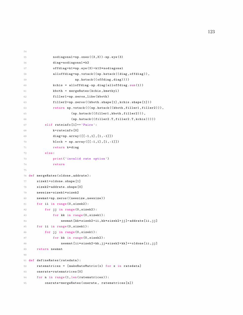
123
54
55 nodiagonal=np.ones ((3,3))-np.eye(3)
56 diag=nodiagonal*k2
57 offdiag=k1*np.eye(3)+k12*nodiagonal
58 alloffdiag=np.vstack ((np.hstack ((diag ,offdiag)),
59 np.hstack ((offdiag ,diag))))
60 kchis = alloffdiag -np.diag(alloffdiag.sum (1))
61 kboth = mergeRates(kchis ,kmethyl)
62 filler1=np.zeros_like(kboth)
63 filler2=np.zeros ((kboth.shape[1], kchis.shape [1]))
64 return np.vstack (((np.hstack ((kboth ,filler1 ,filler2))),
65 (np.hstack ((filler1 ,kboth ,filler2))),
66 (np.hstack (( filler2.T,filler2.T,kchis)))))
67 elif rateinfo [1]== 'Pairs ':
68 k=rateinfo [0]
69 diag=np.array ([[-1,1],[1,-1]])
70 block = np.array ([[-1,1],[1,-1]])
71 return k*diag
72 else:
73 print('invalid rate option ')
74 return
75
76 def mergeRates(oldone ,addrate):
77 sizek1=oldone.shape [1]
78 sizek2=addrate.shape [0]
79 newsize=sizek1*sizek2
80 newmat=np.zeros((newsize ,newsize))
81 for ii in range(0,sizek2):
82 for jj in range(0,sizek2):
83 for kk in range(0,sizek1):
84 newmat[kk*sizek2+ii ,kk*sizek2+jj]= addrate[ii,jj]
85 for ii in range(0,sizek1):
86 for jj in range(0,sizek1):
87 for kk in range(0,sizek2):
88 newmat[ii*sizek2+kk ,jj*sizek2+kk]+= oldone[ii,jj]
89 return newmat
90
91 def defineRates(ratedata):
92 ratematrices = [makeRateMatrix(x) for x in ratedata]
93 onerate=ratematrices [0]
94 for n in range(1,len(ratematrices)):
95 onerate=mergeRates(onerate , ratematrices[n])

124
96 return onerate
97
98 def allContributions(onerate):
99 filler=np.zeros_like(onerate)
100 return np.vstack (((np.hstack ((onerate ,filler ,filler))),
101 (np.hstack ((filler ,onerate ,filler))),
102 (np.hstack ((filler ,filler ,onerate)))))
103
104 def defineRateMatrix(param):
105 pops = param['pop_sim ']
106 for nf in range(0,param['nframes ']):
107 param['ratemats '][nf]. append(len(param['anglemats '][nf]))
108 onerate=defineRates(param['ratemats '])
109 if param['chi?'] and not param['chimethyl?']:
110 if param['all_contributions ']:
111 onerate=allContributions(onerate)
112 nsites=len(pops)
113 oneratematrix=np.zeros ((nsites ,nsites))
114 for x in range(0,nsites):
115 for y in range(0,nsites):
116 if y != x:
117 oneratematrix[x,x]-=2* pops[y]* onerate[x,y]/( pops[x]+pops[y])
118 oneratematrix[x,y]=2* onerate[x,y]*math.sqrt(pops[x]*pops[y])/(pops[x]+pops[y
])
119 return oneratematrix
B.2.2 Site Matrix
Dropbox\HEFCode\oneSiteMatrix.py
1 import math
2 import copy
3 import numpy as np
4 """
5 oneSiteMatrix
6 """
7
8 def defineSiteAngles(param):
9 anglemats=copy.deepcopy(param['anglemats '])
10 """ Convert degree inputs into single frame , radian values """
11 nframes=len(anglemats)
12 oneanglematrix=np.array ([])
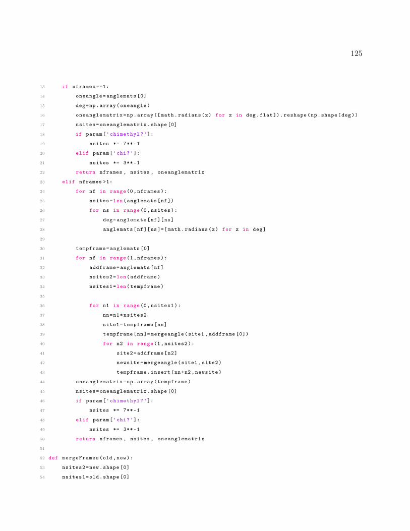
125
13 if nframes ==1:
14 oneangle=anglemats [0]
15 deg=np.array(oneangle)
16 oneanglematrix=np.array([math.radians(z) for z in deg.flat]).reshape(np.shape(deg))
17 nsites=oneanglematrix.shape [0]
18 if param['chimethyl?']:
19 nsites *= 7**-1
20 elif param['chi?']:
21 nsites *= 3**-1
22 return nframes , nsites , oneanglematrix
23 elif nframes >1:
24 for nf in range(0,nframes):
25 nsites=len(anglemats[nf])
26 for ns in range(0,nsites):
27 deg=anglemats[nf][ns]
28 anglemats[nf][ns]=[ math.radians(z) for z in deg]
29
30 tempframe=anglemats [0]
31 for nf in range(1,nframes):
32 addframe=anglemats[nf]
33 nsites2=len(addframe)
34 nsites1=len(tempframe)
35
36 for n1 in range(0,nsites1):
37 nn=n1*nsites2
38 site1=tempframe[nn]
39 tempframe[nn]= mergeangle(site1 ,addframe [0])
40 for n2 in range(1,nsites2):
41 site2=addframe[n2]
42 newsite=mergeangle(site1 ,site2)
43 tempframe.insert(nn+n2,newsite)
44 oneanglematrix=np.array(tempframe)
45 nsites=oneanglematrix.shape [0]
46 if param['chimethyl?']:
47 nsites *= 7**-1
48 elif param['chi?']:
49 nsites *= 3**-1
50 return nframes , nsites , oneanglematrix
51
52 def mergeFrames(old ,new):
53 nsites2=new.shape [0]
54 nsites1=old.shape [0]

126
55 merged=np.zeros(( nsites1*nsites2 ,nsites1*nsites2))
56 for n1 in range(0,nsites1):
57 nn=n1*nsites2
58 merged[nn]= mergeangle(old[n1],new [0])
59 for n2 in range(1,nsites2):
60 merged[nn+n2]= mergeangle(old[n1],new[n2])
61 return merged
62
63 def angle2matrix(angle ,axis):
64 """ For a rotation by 'angle ' (in radians) around an axis ('y' or 'z '), gives the matrix
representation """
65 cos=math.cos(angle)
66 sin=math.sin(angle)
67 if axis is 'z':
68 m = np.array ([[cos ,-sin ,0],[sin ,cos ,0] ,[0 ,0 ,1]])
69 elif axis is 'y':
70 m = np.array ([[cos ,0,sin],[0,1,0],[-sin ,0,cos]])
71 else:
72 print('This does not compute ')
73 m = np.identity (3)
74 return m
75
76 def euler2matrix(angles):
77 """ For a set of Euler angles , given by the Rose convention (z-y-z), generate an array
with the composite rotation. """
78 alpha=angle2matrix(angles [0],'z')
79 beta=angle2matrix(angles [1],'y')
80 gamma=angle2matrix(angles [2],'z')
81
82 m=np.dot(alpha ,np.dot(beta , gamma))
83 return m
84
85 def mergeangle(a1 ,a2):
86 """ Given two sets of Euler angles , a1 and a2, describing sequential transformations (R1
followed by R2, or R2*R1), return the equivalent single transformation."""
87 rot1=euler2matrix(a1)
88 rot2=euler2matrix(a2)
89 rot=np.dot(rot1 ,rot2)
90
91 cb=rot[2,2]
92 if (1-math.fabs(cb)) <=0.00001: #if beta is ~0, it messes up the math. set gamma = 0,
define alpha as single rotation around z axis

127
93 beta=0
94 gamma=0
95 alpha=math.atan2(-rot[0,1],rot [1 ,1])
96 else:
97 beta=math.acos(rot[2,2])
98 if beta <0:
99 beta+=math.pi*2
100
101 alpha=math.atan2(rot[1,2],rot[0,2])
102 if alpha <0:
103 alpha+=math.pi*2
104
105 gamma=math.atan2(rot[2,1],-rot [2 ,0])
106 if gamma <0:
107 gamma +=math.pi*2
108 euler =[alpha ,beta ,gamma]
109 return (euler)
110
111 def chi2euler(chi ,allsites):
112 angle_m1 = []
113 angle_m2 = []
114 angle_d = []
115 for nn in range(0,len(chi [0])):
116 chi1=[math.radians(x) for x in [0, 70.5, -chi [0][nn]]]
117 chi2_m1 =[math.radians(x) for x in [0, 70.5, -chi [1][nn]]]
118 chi2_m2 =[math.radians(x) for x in [0, 70.5, -chi [1][nn] -120]]
119 chi2_d =[math.radians(x) for x in [0, 70.5, -chi [1][nn ]+120]]
120 angle_m1.append ([math.degrees(x) for x in mergeangle(chi2_m1 ,chi1)])
121 angle_m2.append ([math.degrees(x) for x in mergeangle(chi2_m2 ,chi1)])
122 angle_d.append ([math.degrees(x) for x in mergeangle(chi2_d ,chi1)])
123 if allsites:
124 return angle_m1 + angle_m2 + angle_d
125 else:
126 return angle_m1
127
128 def chi2eulerMethyl(chi ,allsites):
129 angle_m1 = []
130 angle_m2 = []
131 angle_d = []
132 md1 = [math.radians(x) for x in [0, 70.5, -60]]
133 md2 = [math.radians(x) for x in [0, 70.5, 60]]
134 md3 = [math.radians(x) for x in [0, 70.5, 180]]

128
135 for nn in range(0,len(chi [0])):
136 chi1=[math.radians(x) for x in [0, 70.5, -chi [0][nn]]]
137 chi2_m1 =[math.radians(x) for x in [0, 70.5, -chi [1][nn]]]
138 chi2_m2 =[math.radians(x) for x in [0, 70.5, -chi [1][nn] -120]]
139 chi2_d =[math.radians(x) for x in [0, 70.5, -chi [1][nn ]+120]]
140 m1=mergeangle(chi2_m1 ,chi1)
141 m2=mergeangle(chi2_m2 ,chi1)
142
143 angle_m1.append ([math.degrees(x) for x in mergeangle(md1 ,m1)])
144 angle_m1.append ([math.degrees(x) for x in mergeangle(md2 ,m1)])
145 angle_m1.append ([math.degrees(x) for x in mergeangle(md3 ,m1)])
146 angle_m2.append ([math.degrees(x) for x in mergeangle(md1 ,m2)])
147 angle_m2.append ([math.degrees(x) for x in mergeangle(md2 ,m2)])
148 angle_m2.append ([math.degrees(x) for x in mergeangle(md3 ,m2)])
149 angle_d.append ([math.degrees(x) for x in mergeangle(chi2_d ,chi1)])
150 if allsites:
151 return angle_m1 + angle_m2 + angle_d
152 else:
153 return angle_m1
B.2.3 Wigner Angles
Dropbox\HEFCode\wignerangles.py
1 import math
2 import numpy as np
3 """
4 wignerangles
5 #==============================================================================
6 # D = wigner(alpha ,beta ,gamma)
7 # Calculates Wigner rotation matrix elements D2_mn
8 #
9 # D 2 1 0 -1 -2
10 # 2 a b c d e
11 # 1 -b f g h d
12 # 0 c -g k g c
13 # -1 -d h -g f b
14 # -2 e -d c -b a
15 #==============================================================================
16 """
17
18 def wignerFull(angle):
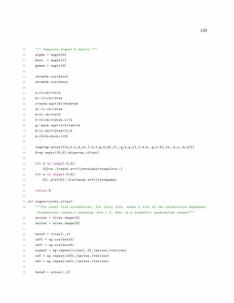
129
19 """ Complete Wigner D matrix """
20 alpha = angle [0]
21 beta = angle [1]
22 gamma = angle [2]
23
24 cb=math.cos(beta)
25 sb=math.sin(beta)
26
27 a=(1+cb)**2/4
28 b=-(1+cb)/2*sb
29 c=math.sqrt (6)/4*sb*sb
30 d=-(1-cb)/2*sb
31 e=(1-cb)**2/4
32 f=(1+cb)*(2*cb -1)/2
33 g=-math.sqrt (3/2)*sb*cb
34 h=(1-cb)*(2*cb+1)/2
35 k=(3/2* cb*cb -1/2)
36
37 temp=np.array ([[a,b,c,d,e],[-b,f,g,h,d],[c,-g,k,g,c],[-d,h,-g,f,b],[e,-d,c,-b,a]])
38 D=np.empty ((5 ,5),dtype=np.cfloat)
39
40 for m in range(-2,3):
41 D[2+m,:]= math.e**(1j*m*alpha)*temp [2+m,:]
42 for n in range(-2,3):
43 D[:,2+n]=D[:,2+n]*math.e**(1j*n*gamma)
44
45 return D
46
47 def wigner(sites ,tiles):
48 """ For every tile orientation , for every site , makes a list of the orientation -dependent
frequencies \omega_i assuming \eta = 0, that is a symmetric quadrupolar moment """
49 ntiles = tiles.shape [0]
50 nsites = sites.shape [0]
51
52 betaT = tiles [:,1]
53 cbT1 = np.cos(betaT)
54 sbT1 = np.sin(betaT)
55 alphaT = np.repeat(tiles [:,0],(nsites ,)*ntiles)
56 cbT = np.repeat(cbT1 ,(nsites ,)*ntiles)
57 sbT = np.repeat(sbT1 ,(nsites ,)*ntiles)
58
59 betaS = sites [:,1]

130
60 cbS1 = np.cos(betaS)
61 sbS1 = np.sin(betaS)
62 gammaS = np.tile(sites[:,2], ntiles)
63 cbS = np.tile(cbS1 ,ntiles)
64 sbS = np.tile(sbS1 ,ntiles)
65
66 x = alphaT + gammaS
67 D = 3/4* sbS **2* sbT **2*np.cos (2*x) -3*sbS*cbS*sbT*cbT*np.cos(x)+(3/2* cbT **2 -1/2) *(3/2* cbS
**2 -1/2)
68 return D
69
70 def wignermas(sitea ,npr):
71 """ Wigner D values for sites and spinning steps """
72 betas = sitea [:,1]
73 gammas = sitea [:,2]
74 cs = math.sqrt (3/8)*np.sin(betas)**2
75 gs = -math.sqrt (3/2)*np.sin(betas)*np.cos(betas)
76 ks = 1/2*(3* np.cos(betas)**2-1)
77 site = np.array ([cs,gs,ks ,-gs ,cs]).T*np.exp(1j*gammas[:,np.newaxis ]*np.linspace(2, -2,
5))
78
79 betam = math.acos (1/ math.sqrt (3.))
80 cm = math.sqrt (6)/4* math.sin(betam)**2
81 gm = -math.sqrt (3/2)*math.sin(betam)*math.cos(betam)
82 km = 1/2*(3* math.cos(betam)**2-1)
83 alpham = np.linspace (0,2* math.pi,num=npr +1)#np.linspace (0,2* math.pi,num=npr+1)#np.append
(np.linspace(0,math.pi,num=npr /2+1),np.linspace(math.pi ,0,num=npr /2+1) [1:]) #]) linspace(
math.pi ,)2*math.pi/npr*(np.arange(0,npr+1))
84 #alpham += alpham [1]/2
85 spinning = np.exp(1j*alpham[:,np.newaxis ]*np.linspace(2, -2, 5))*np.array([cm, -gm ,km,
gm,cm])
86 return site ,spinning
87
88 def wignert1(sites):
89 """ Wigner D values for site orientations needed to calculate the spectral densities , J
"""
90 betaS = sites [:,1]
91 cb = np.cos(betaS)
92 sb = np.sin(betaS)
93 g = sites [:,2]
94 n = np.linspace (-2,2,5)
95 nn = np.exp(1j*np.outer(g,n))
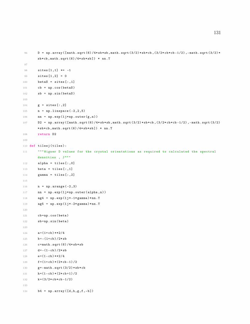
131
96 D = np.array([math.sqrt (6)/4*sb*sb ,math.sqrt (3/2)*sb*cb ,(3/2* cb*cb -1/2) ,-math.sqrt (3/2)*
sb*cb ,math.sqrt (6)/4*sb*sb]) * nn.T
97
98 sites [1,1] *= -1
99 sites [1,2] = 0
100 betaS = sites [:,1]
101 cb = np.cos(betaS)
102 sb = np.sin(betaS)
103
104 g = sites [:,2]
105 n = np.linspace (-2,2,5)
106 nn = np.exp(1j*np.outer(g,n))
107 D2 = np.array([math.sqrt (6) /4*sb*sb,math.sqrt (3/2)*sb*cb ,(3/2* cb*cb -1/2) ,-math.sqrt (3/2)
*sb*cb,math.sqrt (6)/4*sb*sb]) * nn.T
108 return D2
109
110 def tilesj(tiles):
111 """ Wigner D values for the crystal orientations as required to calculated the spectral
densities , J"""
112 alpha = tiles [:,0]
113 beta = tiles [:,1]
114 gamma = tiles [:,2]
115
116 n = np.arange (-2,3)
117 nn = np.exp(1j*np.outer(alpha ,n))
118 ag4 = np.exp(1j*-1* gamma)*nn.T
119 ag5 = np.exp(1j*-2* gamma)*nn.T
120
121 cb=np.cos(beta)
122 sb=np.sin(beta)
123
124 a=(1+cb)**2/4
125 b=-(1+cb)/2*sb
126 c=math.sqrt (6)/4*sb*sb
127 d=-(1-cb)/2*sb
128 e=(1-cb)**2/4
129 f=(1+cb)*(2*cb -1)/2
130 g=-math.sqrt (3/2)*sb*cb
131 h=(1-cb)*(2*cb+1)/2
132 k=(3/2* cb*cb -1/2)
133
134 b4 = np.array([d,h,g,f,-b])
132
135 b5 = np.array([e,d,c,b,a])
136 d4=b4*ag4
137 d5=b5*ag5
138 return d4,d5
B.3 Tiling
Dropbox\HEFCode\zcwtiling.py
1 import math
2 import numpy as np
3 import pickle
4 """
5 zcwtiling
6 number of tiles ---> tile matrix , actual number of tiles
7 """
8
9 def ntiles(n):
10 """ returns fibonnacci number >= n"""
11 a, b = 0, 1
12 while a+b < n:
13 a, b = b, a+b
14 return a,a+b
15
16 def tiles(n):
17 """ returns set of two site ZCW angles , and number of angles """
18 m,n=ntiles(n)
19 tilemat = np.zeros ((n,4))
20 tilemat [:,0] = np.fmod(np.arange(n,dtype=np.float)*m,n)*2* math.pi/n
21 tilemat [:,1] = (np.arange(n,dtype=np.float)+1/2)*math.pi/n
22 tilemat [:,3] = np.sin(tilemat [:,1])
23 return tilemat , n
24
25 def tiles3(n):
26 """ returns set of three site ZCW angles , and number of angles , from pre -saved files """
27 tilesx = pickle.load( open("zcw3.p", "rb" ) )
28 if n <= 200:
29 n = 200
30 elif n<= 300:
31 n = 300
32 elif n <= 538:
33 n = 538
133
34 elif n <=1154:
35 n = 1154
36 elif n<= 3722:
37 n = 3722
38 elif n <= 6044:
39 n = 6044
40 return tilesx[n], n