copyright by wentao fu 2014
TRANSCRIPT

Copyright
by
Wentao Fu
2014

The Dissertation Committee for Wentao Fu Certifies that this is the approved
version of the following dissertation:
A CONCURRENT APPROACH TO AUTOMATED
MANUFACTURING PROCESS PLANNING
Committee:
Richard H. Crawford, Supervisor
Matthew I. Campbell, Co-Supervisor
Wei Li
Benito R. Fernandez
Tolga Kurtoglu

A CONCURRENT APPROACH TO AUTOMATED
MANUFACTURING PROCESS PLANNING
by
Wentao Fu, B.E., M.S.E.
Dissertation
Presented to the Faculty of the Graduate School of
The University of Texas at Austin
in Partial Fulfillment
of the Requirements
for the Degree of
Doctor of Philosophy
The University of Texas at Austin
May 2014

Dedication
To my parents, Andao Fu and Jieying Li.

v
Acknowledgements
I would like to thank Dr. Matthew Campbell for his constant guidance, support
and encouragement during the progress of this dissertation and my graduate study abroad.
It was his excellent research that ignited my enthusiasm in the research direction I am
pursuing. His vision, pursuit of high standard and kindness will continue benefiting my
future development. Also I would like to thank Dr. Richard Crawford for serving as my
supervisor after Dr. Campbell moved to another university. In particular, I am grateful for
his help on finding financial support for me during my last year, without which it would
not have been so smooth for me to finish my research. I wish to thank my committee
members, Dr. Wei Li and Dr. Benito Fernandez, for their valuable input ever since my
qualifying exam all the way to my final defense.
This work is based on a collaborative research project that was led by Palo Alto
Research Center. I would like to thank all my research partners and colleagues, especially
Dr. Ata Eftekharian and Dr. Tolga Kurtoglu, for their excellent work and leadership that
helped make this dissertation possible. Dr. Kurtoglu is also my external committee
member, and I would like to thank him for his service.
I want to thank my family: my sister, my brother, and particularly my father and
mother, Andao and Jieying. They have witnessed me going through all the important
stages through my life and they have always been there to support me, to comfort me, and
to be proud of me.
At the end, I thank my friends in Austin, without whom my life here would not
have been this meaningful. I want to extend special thanks to my girlfriend Suirong, for
not breaking up with me when we were staying apart, for preparing countless tasteful

vi
dishes that have been engraved in my memory, and for travelling with me to every
meaningful place in my life.

vii
A CONCURRENT APPROACH TO AUTOMATED
MANUFACTURING PROCESS PLANNING
Wentao Fu, Ph.D.
The University of Texas at Austin, 2014
Supervisors: Matthew I. Campbell, Richard H. Crawford
With the increasing demand of fast-paced and hybrid manufacturing processes in
modern industry, it is desirable to expedite the iterations between design and
manufacturing through intelligent computational techniques. In this research, we propose
a concurrent approach of this kind to streamline the design and manufacturing processes.
With this approach, a CAD design is automatically analyzed in terms of its
manufacturability in the early design stage. If the part is manufacturable, a set of process
plans optimized in time, cost, fixture quality and tolerance satisfaction are reported in real
time. If the part is not manufacturable, the potential design changes are provided for
better manufacturing.
In the approach, the geometric information of 3D models and the empirical
knowledge in manufacturing processes, fixtures, and tolerances are combined and
encapsulated into a graph-grammar based reasoning. The reasoning systematically
extracts meaningful manufacturing details that later constitute complete process plans for
any given solid model. The plans are then evaluated and optimized using a specially
designed multi-objective best first search technique. The complete approach enables a
concurrent and efficient manufacturability analysis tool that closely resembles real
manufacturing planning practice.

viii
Numerous case studies with real engineering parts are presented to characterize
the novelty and contributions of this approach. The optimality of the suggested plans is
verified through computational comparisons, and the practicality of the plans is validated
with hands-on implementations on the shop floor.

ix
Table of Contents
Table of Contents ................................................................................................... ix
List of Tables ........................................................................................................ xii
List of Figures ...................................................................................................... xiii
Chapter 1: Introduction ............................................................................................1
1.1. Motivation ................................................................................................3
1.2. Technologies and Approaches Involved ..................................................4
1.3. Dissertation Statement .............................................................................5
1.4. Organization .............................................................................................5
Chapter 2: Literature Review ...................................................................................8
2.1. Computer-aided Manufacturing Process Planning ..................................8
2.2. Computer-aided Fixture Design .............................................................11
2.3. Automated Turning Process Planning ...................................................13
PART I: AUTOMATED MANUFACTURABILITY FEEDBACK ANALYSIS 15
Chapter 3: Geometric Reasoning ...........................................................................19
Chapter 4: Graph Grammar Based Reasoning .......................................................23
4.1. Seed Lexicon ..........................................................................................23
4.2. Rule Development .................................................................................30
Chapter 5: Fixture Design and Plan Evaluation .....................................................40
5.1. Defining Fixture Candidates with Graph Grammar ...............................41
5.2. Evaluating Fixture Candidates ...............................................................44
5.3. Plan Consolidation .................................................................................49
Chapter 6: Multi-objective Hierarchical Sorting based Best First Search .............51
6.1. Introduction ............................................................................................51
6.2. Search Hierarchy and Sorting Strategy ..................................................54
6.3. Search Efficiency and Practicality .........................................................57
6.4. Case Studies ...........................................................................................60

x
6.5. Summary ................................................................................................66
Chapter 7: Case Studies and Discussions ..............................................................67
7.1. Radiobox: Dynamic Allocation of Faces For Optimal Fixture Design .67
7.2. Part II: Dependency Between Fixture Design and Manufacturing Process
Planning ...............................................................................................70
7.3. Stabilizer: Synthesized Reasoning Applied in Manufacturing Complicated
Features ................................................................................................75
7.4. Non-manufacturability Analysis ............................................................79
7.5. Characteristics of Implementation and Deployment..............................81
Chapter 8: Part I Summary ....................................................................................83
PART II: AUTOMATED REASONING FOR DEFINING TURNING OPERATIONS FOR
MILL-TURN PARTS 85
Chapter 9: Geometric Reasoning ...........................................................................88
9.1. Detecting the Dominant Rotational Axis ...............................................89
9.2. Defining the Cutting Planes ...................................................................91
9.3. Recovering the Revolving Facet ............................................................92
9.4. Extracting Turnable and Non-turnable Features ....................................93
9.5. Efficiency and Effectiveness ..................................................................94
Chapter 10: Setup Design Based On Tolerance Analysis ......................................96
Chapter 11: Graph Grammar Based Reasoning .....................................................99
Chapter 12: Detailed Example .............................................................................109
Chapter 13: Plan Validation .................................................................................113
Chapter 14: Part II Summary ...............................................................................118
Chapter 15: Conclusion........................................................................................120
15.1. Summary ............................................................................................120
15.2. Contributions and Novelty .................................................................121
15.3. Future Work .......................................................................................123
15.4. Closing Remarks ................................................................................127

xi
Bibliography ........................................................................................................128
Vita… ...................................................................................................................138

xii
List of Tables
Table 1: Labels and their definitions in AMFA grammar reasoning. ..................... 28
Table 2: Description of rule sets and their tasks. .................................................... 31
Table 3: Fixture design guidelines and evaluation metrics. .................................... 45
Table 4: Extreme cases that are penalized in fixture quality measurement. ........... 46
Table 5: All computations needed to form the fixture quality. ............................... 48
Table 6: Comparison between hierarchical search and A* search for example 1. . 60
Table 7: Comparison between hierarchical search and A* search for example 2. . 63
Table 8: An optimal manufacturing plan with fixtures for Radio box. ................... 69
Table 9: An optimal manufacturing plan with fixtures for part II. ......................... 72
Table 10: Comparison between the manufacturing parameters suggested by the
reasoning and the actual choices in the machine shop for part II. ............ 74
Table 11: An optimal manufacturing plan with fixtures for the stabilizer. ............... 76
Table 12: Comparison between the manufacturing parameters suggested by the
reasoning and the actual choices in the machine shop for the stabilizer. . 78
Table 13: The analysis results of the two plans from the tolerance analysis
module…................................................................................................. 116

xiii
List of Figures
Figure 1: Overview of the work presented in the dissertation.................................... 2
Figure 2: Flowchart of AMFA reasoning. ................................................................ 16
Figure 3: Volume decomposition tree. ..................................................................... 21
Figure 4: Part A in Figure 2 as a seed graph. ........................................................... 24
Figure 5: A sample face representation in the seed lexicon. .................................... 25
Figure 6: An example of infeasible tool entry face. ................................................. 33
Figure 7: Another case of infeasible tool entry face. ................................................ 34
Figure 8: (a) Drilling rule 1 for type 1 hole, (b) drilling rule 2 for type 2 hole. ....... 36
Figure 9: Grammar reasoning flowchart in AMFA. ................................................. 38
Figure 10: Downward clamping and side clamping as applied on a work-piece. ...... 42
Figure 11: Screenshot of a rule in rule set 5. .............................................................. 43
Figure 12: Screenshot of another rule in rule set 5. .................................................... 44
Figure 13: A case where the inaccessibility penalty is assigned. ............................... 47
Figure 14: Comparison of two plans with and without consolidation........................ 50
Figure 15: A tree structure of the search space in process planning. ......................... 52
Figure 16: An illustrative part. ................................................................................... 55
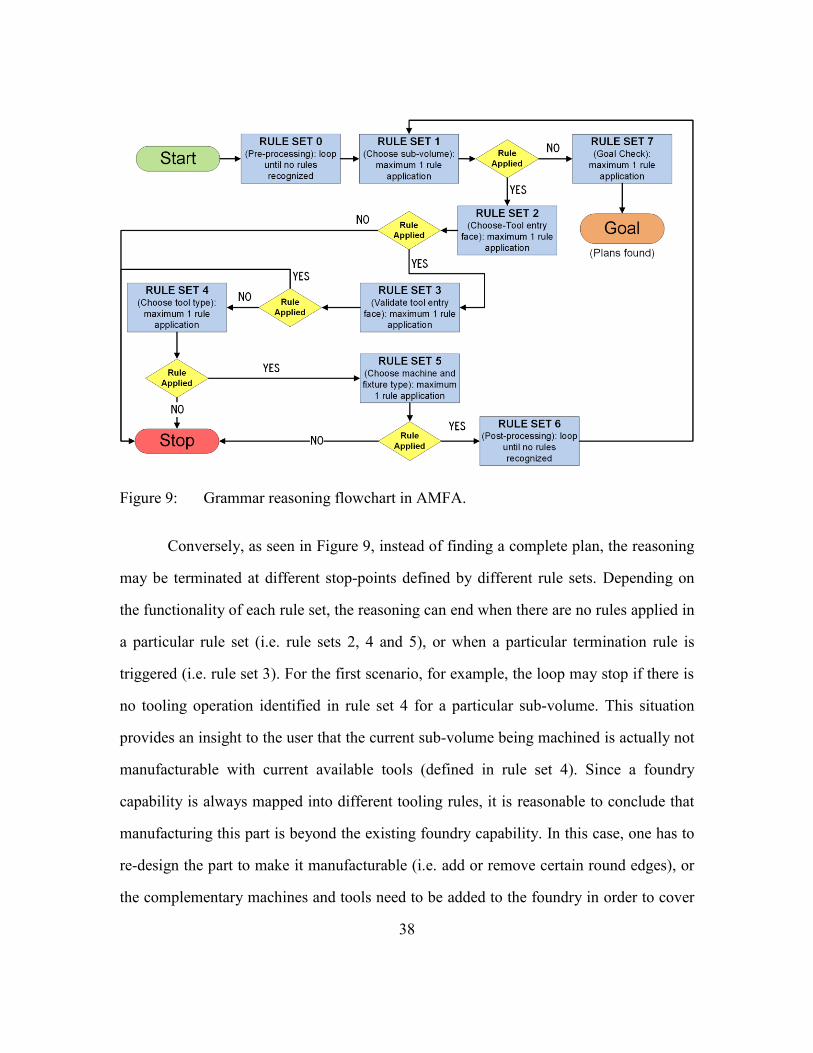
Figure 17: Flowchart of the search algorithm with hierarchical sorting. ................... 57
Figure 18: Example part 1. ......................................................................................... 60
Figure 19: Comparison of two plans for example 1. .................................................. 62
Figure 20: Example part 2. ......................................................................................... 63
Figure 21: The optimal plan generated by hierarchical search for example 2. .......... 64
Figure 22: The plot of computational time versus part complexity. .......................... 65
Figure 23: Summary of the exhaustive search for the part in Figure 16. ................... 66
Figure 24: CAD model of the “Radio box”. ............................................................... 67
Figure 25: CAD model of part 2................................................................................. 71
Figure 26: CAD model of the stabilizer. .................................................................... 75

xiv
Figure 27: (a) A non-manufacturable part due to design flaws, (b) the machined part
simulated in FeatureCAM, and (c) the manufacturability analysis result
generated in AMFA. ................................................................................. 80
Figure 28: A sample manufacturing plan generated in FeatureCAM. ....................... 80
Figure 29: A sample AMFA GUI. .............................................................................. 81
Figure 30: A sample part with non-turnable features. ................................................ 88
Figure 31: (a) The identified curved edges and (b) their axial normal vectors for the
part in Figure 30. ....................................................................................... 91
Figure 32: A unit circle with non-uniform radial vectors........................................... 92
Figure 33: (a) The sampled cross sections of the part in Figure 30; (b) the union of all
the cross sections....................................................................................... 93
Figure 34: (a) The revolving face and the rotational axis; (b) the as-lathed model. .. 93
Figure 35: (a) The decomposed turnable features; (b) the non-turnable features. ..... 94
Figure 36: A summary of the tests on more complex parts. ....................................... 95
Figure 37: Grammar reasoning flowchart for turning process planning. ................. 100
Figure 38: The CAD drawing of the part shown in Figure 34b. .............................. 100
Figure 39: The tolerance graph generated from the 2D drawing in Figure 38. ........ 101
Figure 40: The generalized angle of the parallelism tolerance. .......................... 102
Figure 41: The screenshot of (a) rule 1, (b) rule 2 and (c) rule 3. ............................ 105
Figure 42: The screenshot of the setup graph. .......................................................... 106
Figure 43: The suggested turning sequence for the part shown in Figure 34b......... 108
Figure 44: A complex part with interacting features. ............................................... 109
Figure 45: The CAD drawing of the as-lathed model in Figure 44a. ....................... 110
Figure 46: The tolerance graph for the part shown in Figure 44a. ........................... 110
Figure 47: The updated tolerance graph for the part shown in Figure 44a. ............. 111
Figure 48: The setup graph for the part in Figure 44a. ............................................. 112
Figure 49: The suggested turning sequence for the part shown in Figure 44a. ........ 112
Figure 50: A traditional turning sequence for the part shown in Figure 34b. .......... 115
Figure 51: 2D contour tool path. .............................................................................. 124

xv
Figure 52: The zig-zag tool path projected onto a milling surface. .......................... 124

1
Chapter 1: Introduction
Computer-aided manufacturing process planning (CAMPP, also known as CAPP)
is a broad research topic as it sees applications in disassembly [1], assembly [2], and
machining [3], [4]. In this work, we present systematic approaches to solving the
manufacturing process planning problems. As shown in Figure 1, we start with an input
CAD model. Then the geometric reasoning that was developed by Eftekharian et al. [5],
[6] analyzes the part in order to identify the turnable and non-turnable features that need
to be created. For non-turnable features that require milling, drilling and other non-
turning material-removal processes (also referred to as subtractive manufacturing
processes), a tool known as Automated Manufacturability Feedback Analysis (AMFA)
[3], [7], [8] has been developed to automatically generate process plans that are
optimized in manufacturing time, cost and fixture quality. Each optimal plan is detailed
with suggested tools, feed directions, machines, and fixtures in order to complete the
machining of the part. For turnable features, a tolerance based algorithm presented in [6],
[9] is used to propose feasible turning process plans that best comply with the design
tolerance specifications. Both process planning algorithms are developed based on the
graph grammar, and are referred to as Grammar Reasoning in the flowchart. This
dissertation focuses on the grammar reasoning as it is the major contribution of the
author. In addition, since the geometric reasoning serves as an important module to this
work, we will give moderate explanation when necessary.
As indicated in Figure 1, the research is split into two parts depending on the
types of feature identified from the input CAD model. For the non-turnable features, the
relevant geometric reasoning and grammar reasoning have been integrated into AMFA,
which is part I of this dissertation. The geometric reasoning and grammar reasoning

2
relevant to the turning process planning are introduced together in part II of this
dissertation.
Figure 1: Overview of the work presented in the dissertation.

3
1.1. MOTIVATION
Modern manufacturing industry is motivated to reduce time and cost in order to
keep competitiveness. The main hurdle is the unnecessary back-and-forth between the
design and manufacturing due to a lack of thorough understanding of a product in terms
of its manufacturability in the early design phase, which often leads to additional time
and cost for design iterations and manufacturing process improvements. The
computational approach proposed in this research is aimed at alleviating this problem. In
this technique, the manufacturability analysis is customizable based on a specific foundry
capability, and a CAD design is assessed automatically and efficiently in terms of every
detail of the manufacturing processes. The automated reasoning expedites the
communication between design and manufacturing, and facilitates the designer to make
judicious decisions in how to improve the design for better manufacturing and to get a
sense of how to manufacture the part for lowest time and cost during the product
development.
To reduce the manufacturing time and cost, the traditional process planning relies
heavily on the shop-floor experience, which is very difficult to interpret computationally.
Existing commercial CAD/CAM packages such as FeatureCAM [10] require numerous
pre-decisions made by the user (e.g. the orientation of the raw-stock, the available tools
and machines) before a process plan can be generated. The reported plan is therefore
subject to change with the user customization and the optimality is not guaranteed. The
dissertation aims to break through such limitations in current manufacturing practice by
introducing the notion of a design space in which all possible process plans are generated
for a given solid model. The integrated search technique constantly traverses the space in
order to find the best plans that are guaranteed to be optimal in terms of the user-specified
objectives.

4
The concurrency of the proposed approach stems from the fact that manufacturing
process planning overlaps with the knowledge of several disciplines. The interaction
between one aspect and another (e.g. the effect of fixture design on the time and cost
estimation of a process plan, and the interaction between the sequence of machining
operations and the corresponding fixture designs) needs to be carefully assessed before a
conclusion of the optimality of a process plan can be made. In our algorithm, the multi-
disciplinary knowledge relevant to the process planning is considered “on the fly” so that
the reasoning is constantly informed of the direction towards defining the empirical and
optimal process plans.
1.2. TECHNOLOGIES AND APPROACHES INVOLVED
The graph grammar based approaches perform the process planning for turnable
and non-turnable features on a graph grammar platform known as GraphSynth [11] that
was developed by Campbell. It provides a library of graph elements and data structures
that the author uses to design graphs and grammar rules in order to store and capture
relevant geometric and manufacturing knowledge in the reasoning.
For the fixture design in AMFA [8], we use the knowledge gathered from the
shop floor and the engineering handbooks to directly inform the reasoning of optimal
fixture mechanisms for a given tooling operation. In this way, the complicated multi-
objective optimization problem in the fixture design phase is avoided. The resulting
fixture mechanisms are proven to be optimal and implementable.
The planning search technique developed in AMFA is a multi-objective
hierarchical sorting based best first search [8]. It incorporates the manufacturing
knowledge in the otherwise naïve search process and is able to converge to optimal
process plans in manufacturing time, cost and fixture quality in near-linear time. As

5
compared to the traditional A* search, this technique generates more practical process
plans in a much shorter computation time.
A novel tolerance based technique [6], [9] is proposed to define the turning
process plans that better satisfy the tolerance specifications. The idea is to identify the
design knowledge conveyed by the tolerances and encapsulate it into the grammar
reasoning such that the tolerances can be directly and effectively used to guide the
generation of optimal turning sequences.
A tolerance analysis module for validating manufacturing process plans that was
developed by the author and colleagues from Palo Alto Research Center [12] is employed
to compare the suggested turning sequences with manually proposed plans. The result is
used to validate the optimality of our plan in satisfying the prescribed tolerances.
1.3. DISSERTATION STATEMENT
A concurrent approach encapsulating the knowledge of manufacturing, fixture,
tolerance analysis, graph grammars, and tree search optimization automatically defines
optimal manufacturing process plans in terms of manufacturing time, cost, fixture quality
and tolerance satisfaction for any solid model.
1.4. ORGANIZATION
The dissertation is organized as follows. Chapter 2 explores the existing research
in the three major topics of this dissertation: the computer-aided manufacturing process
planning, the computer-aided fixture design and the automated turning process planning.
After this, the dissertation is separated into two parts. The first part is the automated
reasoning for non-turning operations, which includes chapter 3 through chapter 8. In this
part, we explain in detail the automated process planning algorithm, the fixture design
and the search optimization. Chapters 9 to 14 constitute the second part of this

6
dissertation, in which the automated reasoning for defining turning operations is
presented. More specifically:
Part I:
Chapter 3 briefly introduces the geometric reasoning in AMFA done by
Eftekharian et al. As it is not the author’s work, only a high-level description of the
algorithm is provided to ease the understanding of the following chapters.
Chapter 4 describes the graph representation of the solid model and the grammar
rule based reasoning for generating process plans.
Chapter 5 explains how the candidate fixtures for a machining operation are
generated using grammar rules and how the complete plans are evaluated against
specially designed metrics.
Chapter 6 presents a hierarchical sorting based best first search that is developed
to solve the multi-objective optimization problem during the process planning.
Chapter 7 provides three case studies to validate the novelty, effectiveness and
efficiency of our approach. The practicality of the proposed plans is validated through
real implementations in the machine shop.
Chapter 8 summarizes the work in the first part.
Part II:
Chapter 9 provides the geometric reasoning developed by Eftekharian that is used
to identify the turnable features from a mill-turn part. The features are converted to a
graph representation for the later grammar reasoning to work on.
Chapter 10 explains the fundamentals of the turning setup design based on
tolerance analysis.

7
Chapter 11 describes the graph grammar based implementation of the setup
design algorithm through an illustrative case study.
Chapter 12 provides a more complex and detailed example to further explain the
grammar reasoning.
Chapter 13 introduces briefly a tolerance analysis module that the author
developed with Palo Alto Research Center and uses this algorithm to validate the
suggested turning sequences in satisfying prescribed tolerances.
Chapter 14 summarizes the research in part II.
The dissertation closes with chapter 15, which highlights the contributions of this
dissertation. It also outlines the future directions along which the work can be further
improved.

8
Chapter 2: Literature Review
Our research contributes to three major areas: the computer-aided manufacturing
process planning, the computer-aided fixture design, and the automated turning process
planning. Previous work in the three areas is explored in this chapter. For the search
technique and the evaluation of process plans in part I and the tolerance analysis in the
turning process planning, the relevant work is embedded into corresponding chapters for
a better elaboration.
2.1. COMPUTER-AIDED MANUFACTURING PROCESS PLANNING
Computer-aided manufacturing process planning (CAMPP, or CAPP) was first
proposed by Russell [13] in 1967. Due to the fast development since the 1980s, this topic
continues to receive considerable attention both from researchers and engineers. At this
time, many knowledge based approaches [14]–[16] were developed to capture the basics
behind process planning. Marri et al. [17] provided a comprehensive review of these
CAPP systems. They concluded that more attention should be paid to the architecture and
constraints behind machining operations while developing a comprehensive CAPP
system. More recently, Sharma and Gao [18] proposed a process planning system that
employs the up-to-date tools and technologies consistent with the international standard
for exchange of product data (i.e. the .STEP format1). However this system is only
intended for simple prismatic models and the feedback cannot be automatically imported
into CAD systems for detailed re-design. Allen et al. [19] developed an agent-based
approach that provides a number of generic solutions while maintaining the ability for
manual intervention in order to establish local working preferences. However, the
efficiency of this algorithm is restricted by its parametric optimization structure.
1 (.STEP) is used as the standard format for the exchange and conversion of solid models.

9
In contrast, the graph grammar based approach to automated manufacturing
planning, in principle, can support a larger variety of topologies and is not necessarily
restricted by any optimization process. It utilizes a technique of creating new graphs from
an original graph (host) by applying prescribed rules onto the host [20]. The rules are of
the form (L-to-R) where the left hand side (LHS) includes elements and conditions to be
recognized and satisfied in the host graph and the right hand side (RHS) indicates the
transformations of those elements.
A well-known grammar based approach in automated manufacturing planning
uses Form-Feature Recognition (FFR) technique [21]. FFR is primarily important
because it can extract or generate higher level and meaningful geometric primitives [22]
(for example, lines, polygons, triangular facets, et al.) that are not easily inferable from
the 3D geometry. These geometric features serve as a bridge between the geometry on
one hand and manufacturing reasoning on the other hand [23]. Thorough surveys of
various techniques in form-feature recognition can be found in the work by Han et al.
[24], Shah [25], [26], Subrahmanyam [27] and Babic et al. [28]. According to these
surveys, three dominant techniques – graph based, rule based and hint based approaches
– are mostly used in modern FFR algorithms. Graph based techniques, although proven
to be reliable in recognizing isolated features, mainly suffer from the complexity of
geometries and the fact that features may have interactions with each other [29], [30].
Some researchers [31] have tried to tackle the problem by introducing various types of
heuristics to the algorithm and have gained considerable achievements, but still the
problem remains unsolved for complex geometries. Others [29], [32] have tried to add
missing elements that correspond to interacting features into the graph, but despite the
added complexity they do not completely solve the problem. In addition, many

10
contemporary recognition systems deal only with orthogonal features [33]–[36], but little
attention has been paid to non-orthogonal and arbitrary features [37].
Volumetric decomposition methods stand apart from the others, both in the
algorithm employed and the results. Researchers have continued to extend and refine this
approach to solve numerous shortcomings, such as non-convergence and geometric-
domain restrictions. The volumetric decomposition method can handle interactions and
provide additional information such as geometry-based precedence relations [38].
Methods that are most related to our approach use the concept of convex-hull and set-
difference operations to generate meaningful features suitable for machining processes.
The idea is raised from the complicated concept of B-rep to CSG (Constructive Solid
Geometry) conversion discussed in a number of early CAD research works [39]–[41].
Woo [42] proposed a method based on this idea known as Alternating Sum of Volumes
(ASV). One problem in his decomposition approach is the possibility of non-
convergence, which means that the decomposition will never stop unless terminated by
the user for certain geometries. It significantly limits the applicability of this approach.
Kim [43], [44] proposed a technique to overcome this limitation by using a new
partitioning strategy and combining that with the ASV idea mentioned above. The new
method – referred to as ASVP –shows better convergence than ASV but cannot guarantee
the optimality of generated machining features. Another similar approach to this work
was provided by Ertelt and Shea [45]. In this method a vocabulary of removal volume
shapes (or the so-called shape grammars) is used to encode the knowledge of
fundamental machine capabilities. Shape grammars may include available tool dataset,
machines, tool motion information, etc. Since this approach uses topological reasoning
and parametric evaluation concurrently, its scalability to handle parts with increasing
complexity and non-traditional machining processes is questionable.

11
2.2. COMPUTER-AIDED FIXTURE DESIGN
Computer-aided fixture design (CAFD) has been a challenging task for several
reasons. First, a fixture is proposed based on the assessment on factors across different
fields. For example, it relies on the available type of fixtures (either modular or dedicated
fixture) and is specific to particular manufacturing processes [46]. Also a proper fixture
has to provide enough constraints to secure the part under unknown cutting forces.
Additionally, it should not block any potential feed directions or tool paths that are
determined by the geometry of the part as well as the manufacturing procedures. While a
human being with experience thinks of this multi-objective problem naturally, the
computational approaches nowadays still lack the ability to consider these factors as a
whole [47].
Numerous articles can be found in CAFD with each based on a particular topic.
Sermsuti-anuwat [48] proposed a tolerance based approach for milling fixture design, and
Kang et al. [49] generalized the tolerance analysis technique to any type of fixture design.
Pang and Trinkle [50] and Kang et al. [51] approached the fixture design problem by
characterizing the stability of the work-piece. Fan et al. [52] attempted to establish a
service-oriented architecture (SOA) in fixture design in order to facilitate the
communication between various assemblies. Another popular approach is based on the
form closure theory [53], [54], which has been introduced and developed since 1980s.
The idea is that for any given shape in 3D space, there exist 7 frictionless points of
contact that are necessary and sufficient to hold and secure the object under whatever
external forces. With this theory, the problem of fixture design reduces to the selection of
7 points on the part surfaces. Researchers have been actively investigating algorithms to
define the point configurations in [55]–[57].
12
Meanwhile, different techniques have been developed for fixture designs in
distinct applications. The modular fixture provides reconfigurable setups that can be used
for various purposes (e.g. parts of different sizes and shapes). One popular modular
fixture is the reconfigurable pin-array fixture technology [58]. The modular fixture design
has also been studied with intelligent algorithms [59] and sees successful applications in
various environments [60], [61]. In contrast, more complicated or precise manufacturing
processes require dedicated fixtures, for which case-based reasoning (CBR) [62]
techniques have been applied to automate the fixture design process.
Reviews of the aforementioned techniques as well as existing computerized tools
are given in [46], [63]–[65]. In light of the variety of research, Rong et al. [66] proposed
a basic framework for fixture design in order to better streamline the CAFD processes,
where the existing techniques were benchmarked against four main stages: setup
planning, fixture planning, fixture unit design and verification. According to their
investigation, most of the existing work is not able to perform the fixture verification.
One reason is that the fixture analysis has not been thoroughly studied in the context of
manufacturing process planning. This is critical considering that the fixture for a given
operation may need adjustments based on how the operation is sequenced in a
manufacturing plan. It is possible that for a certain operation we want a “sub-optimal”
fixture (e.g. less convenient, relatively harder to set up) in order to ease the operations
that follow.
The fixture design technique proposed in this work is derived from the
manufacturing perspective and is fully embedded into our manufacturability analysis
tool. As to be presented, the reasoning is seamlessly synthesized with the other modules
in grammar reasoning and therefore the optimal and more empirical plans can be found
while the efficiency is preserved.

13
2.3. AUTOMATED TURNING PROCESS PLANNING
In the geometric reasoning of the turning process, Tseng and Joshi [67] developed
a method to extract rotational and prismatic features from mill-turn parts. According to
this work, cylindrical features are extracted by using a sweep-type process where a 2D
profile is first established and then swept around an axis of rotation. One drawback is that
this method requires the axis of rotation to be known therefore is not very suitable for
automatic feature extraction. Kim et al. [68] developed a feature recognition system that
used convex decomposition to decompose the mill-turn parts into a series of negative
machining volumes. They also utilized this method to determine precedence relationships
for machining features. However, their method requires a positive stock volume to be
known a priori.
In automatic generation of machining plans, a small body of literature has been
devoted to turning operations in contrast to milling and CNC machining. In general,
reasoning about turning operations mainly includes two approaches: parametric based
and feature based. Berra and Barash [69] proposed an automatic reasoning scheme for
process planning and optimization of a turning operation. In this work, various turning
parameters were tuned in order to achieve the minimum time and cost associated with
manufacturing. In terms of generating accurate plans (while considering time and cost)
this work lacks incorporating tolerance relationships of various features. Lai-Yuen and
Lee [70], Zhang et al. [71], and Huang et al. [72] have implemented a more
comprehensive algorithm by using various approaches including an activity-based
approach, a surface-roughness approach and an engineering knowledge approach to
model and analyze the turning process. Although they have achieved considerable
improvements, the completeness and accuracy of their methods are still controversial, as
none have studied the tolerance specifications and its effect on the setup design.

14
Feature-based techniques in turning operations have shown to be more accurate in
generating optimal manufacturing plans. Culler [73] developed a feature based intelligent
process planner known as Turning Assistant (TA), which perceives the precedent
knowledge built into the rules and prescribes necessary operations accordingly for each
feature that requires NC lathe work. Similarly, Liu [74] presented a method for the
feature extraction and classification of rotational parts. But according to these papers, not
all forms of the features can be recognized by these approaches. In a different technique,
Suliman and Awan [75] developed a turning feature recognition technique directly from
2D drawings. Although this is an important technique, the validity and applicability in
various models are still to be verified, as the 2D feature recognition is trivial and not
generic enough for use in non-prismatic 3D geometries.
Additionally, it is revealed from the past literature that the feature-based
techniques generally suffer from the feature interactions and the fact that turnable and
non-turnable features may have interference with each other. To solve this problem, Li
and Shah [76] attempted to automatically separate the coupled portions and detect the
form features as well as user-defined features via a graph and rule based recognition
algorithm. But the approach imposes constraints on the shapes that can be processed due
to the missing of certain graph elements. In contrast, this work proposes a new technique
to effectively de-couple features in complex mill-turn parts and generate manufacturing
plans based on tolerance considerations, which is lacking in previous literatures.

15
PART I: AUTOMATED MANUFACTURABILITY FEEDBACK
ANALYSIS
In order to better streamline the interaction between computer-aided design and
manufacturing, an approach is provided which automatically reasons about a CAD model
to define detailed and optimal manufacturing plans. The larger system is known as
Automated Manufacturing Feedback Analysis (AMFA), and this part presents the graph
grammar based reasoning that serves at the system’s foundation. Starting from a seed
graph that represents a CAD model, the grammar reasoning performs the analysis of
manufacturability by referencing the data provided for the manufacturing facility that will
build the part in question. The outputs of AMFA are optimal manufacturing plans, their
associated times and costs, and, in certain cases, recommendations to the designer on how
to change the part for better manufacturing.
To generate the outputs, two distinct efforts are involved, which are referred to as
Geometric Reasoning and Grammar Reasoning as shown in Figure 2. In geometric
reasoning, first a CAD model in the STEP format (Part A in Figure 2) provided by
designers is loaded. Then the geometry – comprised of vertices, edges, and faces – is
translated into a label-rich graph which serves as the basis for the grammar reasoning (the
lower portion in Figure 2). During the translation, a bounding box (Part B in Figure 2) is
extrapolated from the original part A since one would likely start the actual
manufacturing from a bounding raw stock. Then the original part A is subtracted from the
bounding box B to create the negative volume (Part C in Figure 2) that is to be removed.
The removal volume then undergoes further decomposition in order to generate compact
sub-volumes where each is assumed to be machined in one operation or to be tagged as
non-manufacturable. Finally the decomposed removal volume (negative solid) is
converted to a graph, which is used as the initial seed in the grammar reasoning.

16
Figure 2: Flowchart of AMFA reasoning.
In the grammar reasoning, eight sets of grammar rules are invoked in a prescribed
sequence in order to map specific elements that are detected in the seed graph to certain
manufacturing details. This process continues recursively until all feasible manufacturing
operations for the part are defined. The grammar rules reason about the manufacturability
under certain foundry capabilities. First, all available manufacturing processes within a
production facility are translated into grammar rules. The rules are then organized to

17
reason about the seed graph in order to determine its machining details. A search tree is
drawn in Figure 2 to describe the reasoning. Steps in the tree represent alternative
manufacturing operations for different sub-volumes. These operations are determined
through the rules which detect prescribed graph elements in the seed and relate them to
particular manufacturing processes. Each operation consists of the tool entry face, the
feed direction, the tool type, the machine choice, and the proper fixture to machine one
sub-volume. As the tree grows, more and more sub-volumes are effectively removed.
This procedure continues recursively until there are no more sub-volumes available for
machining, and a complete search space that includes all alternative manufacturing plans
for the given part is derived. In addition, by translating the given foundry capability into
graph grammar rules, a precise conclusion of non-manufacturability of a part can be
made if the rules fail to find a feasible plan for this part. It signals that the manufacturing
process is beyond the foundry capability and this part needs to be redesigned.
The geometric and grammar reasoning in AMFA is based on the following
assumptions:
1) After decomposition of the negative solid, each of the resulting sub-volumes is
assumed to be machined in one operation or to be non-machinable. Since the
decomposition cuts the negative solid into a collection of convex sub-volumes, each sub-
volume represents a simple geometric shape (i.e. a cuboid, a cylinder, or a trapezoidal
shape), which can be mapped directly to a tooling operation. For instance, a negative
cylinder is a hole that can be created in a drilling operation, and a negative cuboid can
refer to a pocket that is machined in one milling operation.
2) Tolerance is not considered in this reasoning of non-turning operations (i.e.
milling, drilling, sheet-metal cutting, etc.). The high-level manufacturing plan generated
from the reasoning provides a quick insight into how the profile of the input model can be

18
roughly created. It does not cover the final finishing processes, in which the tolerance
information starts to be critical in deciding the tooling sequence in order to precisely
create the final shape.
3) If a part is not manufacturable because of inaccessible regions (e.g. inner sharp
edges) or unrecognized or invalid geometric elements (e.g. an edge with more than two
vertices), then this part would always be tagged as non-manufacturable in the reasoning
until the required redesign modifications are made by the users.
The following chapters in this part explain the geometric reasoning, the grammar
reasoning, the fixture design, the plan evaluation, and the search optimization of the non-
turning process planning algorithm. Case studies are incorporated into the description for
better understanding. A summary of the characteristics and contributions of the work in
this part is provided at the end.

19
Chapter 3: Geometric Reasoning
This chapter briefly describes the geometric reasoning that was developed by
Eftekharian et al. [5]. As an upstream module of the overall system, the geometric
reasoning in AMFA is customized by the grammar reasoning such that all necessary
information required by the grammar reasoning is extracted from the CAD model and is
passed to the grammar reasoning. While the author was not involved in the development
of this module, a moderate introduction here will facilitate the explanation and
understanding of the grammar reasoning.
In the context of CAPP, the volume decomposition is important and useful for
generating simple removal volumes from the initial work-piece. These sub-volumes are
commonly referred to as machining features in literature. In theory, a decomposed solid
can be represented as the sum of sub-volumes in a hierarchical order that forms a
complete object obtained from its boundary representation (B-rep). In this work we
extend the idea of volumetric decomposition for 3D solid models by adding a level of
reasoning to the algorithm. Our decomposition algorithm uses a ranking strategy to
prioritize concave-edges, in which three heuristics are defined to evaluate the direction of
cut for each division. As shown in Figure 3, the process of volume decomposition can be
represented as an AND/OR tree [77] structure with branching factor equal or greater than
2 (2 is the case when there are exactly two solids generated after each cut) and the depth
of the tree equal to the total number of concave edges in the solid. Each node represents a
volume that needs to be cut and each branch represents a left (L) or right (R) cut in the
tree. Nodes can refer to simple shapes (contain no concave edges) that are represented as
(S) in the tree or complex shapes (contain one or more concave edges) that are
represented as (C) in Figure 3. It is important to note that the “left” and “right” are

20
arbitrary names for the two faces that meet at each edge and they provide the reference
cutting directions for decomposing the larger solid. Both options for slicing are evaluated
to determine which direction (left or right) yields a better decomposition. The evaluation
is based upon three heuristics as summarized below.
Heuristic 1: For both cuts (L versus R), if there are equal concavities in the
resulting sub-volumes, prefer the one that leads to less volume difference. This method is
responsible for cutting the solid in a direction that leads to more equally sized sub-
volumes.
Heuristic 2: For both cuts, if the resulting volumes are non-convex, prefer the
one (L versus R) that leads to fewer overall concave edges within the resulting sub-
volumes.
Heuristic 3: For cuts that produce blind faces that an external tool cannot reach,
the Visibility Test Analysis (VTA) is implemented. This heuristic prefers the cut (L
versus R) that creates fewer (ideally zero) faces that are invisible from outside.

21
Figure 3: Volume decomposition tree.
For a given solid model shown on the top of Figure 3, consider a case where the
left branch is always chosen as the preferred cut, and the results after the first cut could
be one complex (C) and one simple (S) volume (as in Figure 3). The simple volume does
not need any further cutting operations so the branch after this node is terminated: this is
indicated as a red node in the tree. For each complex volume (C) the branch propagates
further to lower levels until it is terminated at simple volumes (S). In order to find an
optimal decomposed solid for use in the grammar reasoning, one can generate all the
possible options in the tree and evaluate each individual option. This, however, is not

22
realistic since the Boolean operations are computationally expensive. Furthermore, the
evaluation conceptually requires a human to inspect the result and decide if it is a good
decomposition (computationally evaluating the quality may be possible, but it is out of
the scope of the work). The alternative solution is to expand a single but promising
branch. At each level of the tree the algorithm evaluates the options and decides the
preferred direction to the next level. This continues until no more complex volumes are
detected. It is important to note that a desired solution is described as a decomposed
volume that contains sub-volumes which are suitable for manufacturing. In other words,
each sub-volume should possess the following properties: 1) it should be of a compact
shape with no or few concavities, 2) it should have a prismatic or close to prismatic
geometry and 3) it should be machinable in one machining operation. Due to the lack of
space, details about the algorithm are omitted here and we refer the interested reader to
[5]. Based on the aforementioned heuristics, only desirable branches will survive and
continue to grow until no further concave edges are recognized. The final decomposed
shape is a combination of all remaining S-type volumes in the decomposition tree. The
decomposed solid at the bottom of Figure 3 is a sample result after the heuristic-guided
volume decomposition of the input solid model.

23
Chapter 4: Graph Grammar Based Reasoning
In this chapter, we explain in detail how the input 3D geometry and the non-
turning operations are represented with graph grammar using GraphSynth. Section 4.1
presents the seed lexicon that uses the graphical elements (e.g. nodes, arcs, and
hyperarcs) to capture all geometric information of the input model that is relevant to
manufacturing process planning. The machining operations are translated into specially
designed grammar rules, which then perform process planning reasoning as illustrated in
section 4.2.
4.1. SEED LEXICON
After the removal volume (negative solid) of a given solid model is decomposed,
the compound solid comprised of different sub-volumes has to be translated into a seed
graph such that the grammar reasoning can reason on it. Rather than using existing graph
techniques to represent a solid model, a new lexicon is proposed in this work. Figure 4
gives an example showing how part A in Figure 2 is represented as a label-rich graph.
This is a simple shape with a pocket in front and a through hole on the back. In
the seed graph, geometric elements are described by nodes, arcs, and hyperarcs. Nodes
are used to represent vertices and faces. Arcs are used to represent edges as well as to
indicate relative positioning information (i.e. parallelism, perpendicularity, etc.) between
any two faces. A hyperarc is a special graph element in GraphSynth. While an arc can
only connect two nodes, a hyperarc can connect as many nodes as needed. In the seed
lexicon, it is used to connect all vertices belonging to a face to their face node. Figure 5
gives an example of a graph representation for a face with four vertices. The node 0
(indicated as n0) with label “face” and “accessible” represents a face that is exposed for
the tool to enter. The other four nodes (n1, n2, n3, and n4) represent all the vertices of

24
this face. They are connected by hyperarc 0 (ha0), which also has label “face” and
“accessible”. The labels are used to distinguish a hyperarc that defines a face from the
one that defines a volume (described below) in the lexicon.
Figure 4: Part A in Figure 2 as a seed graph.

25
Figure 5: A sample face representation in the seed lexicon.
Another type of hyperarc is defined to encompass a sub-volume by connecting all
the nodes in a sub-volume together. The nodes can be the face nodes as well as the nodes
denoting vertices. For example, in Figure 4, the hole and the bottom cuboid are separated
by two hyperarcs. By using nodes, arcs, and hyperarcs in the seed graph, all geometric
information about vertices, edges and faces for a solid model is stored and mapped to the
graph. The face nodes are used in the seed and rules to refer to machining features, like
holes, pockets and slots, if applicable. Mapping edges and vertices to graph elements
provide more detailed information about shapes and geometries, which is essential for the
rules to be able to reason about manufacturing operations more precisely.
It is also important to note that a variety of labels in the graph that are assigned in
the geometric reasoning are used to store topological, rather than parametric, information.
By reasoning about the labels selectively, the grammar reasoning can extract enough

26
information for the manufacturability analysis for a given geometry. As a result, the
geometric computations can be avoided in the grammar reasoning.
For example, a face node may have a label “bb”, which indicates that this face is
a bounding box face. When a face node represents a face that belongs to the removal
volume, it is assigned the label “neg”. For instance, in Figure 4, the face node 1 (n1) (not
explicitly shown, but overlaps with its face hyperarc ha1) representing the bottom face of
the cuboid has a label “neg”, while face n12 has a label “bb”. Besides, the face
adjacency property – “convexity” or “concavity” – between any two adjacent faces is
also stored in the label of their common edge. These labels are essential to inform the
search of feasible machining operations for a given sub-volume.
Another important function of labels is to guide the sequencing of machining
operations for different sub-volumes. The following labels are designed to support this
functionality. First, a hyperarc that denotes a face will have a label “accessible” if the
face is reachable by the tool. Such face is a candidate for the tool to enter. Examples can
be found in hyperarcs ha1 and ha9 in Figure 4 and hyperarc ha0 in Figure 5. Second, for
a given face, if its entire area is shared by more than one sub-volume, the face hyperarc
that represents this face will be given a label “common”. When it comes to the case
where only a partial area of this face is common with other sub-volumes, the specific
portion, which is represented by a new hyperarc, will have the “common” label. An
example can be found in the hyperarc ha7 in Figure 4, where it represents the internal
circular face of the hole that is shared by the bigger face of the cuboid that the hole sits
on. The idea of the sub-volume removal sequencing is that: 1) a sub-volume is
manufacturable from only its accessible faces; 2) after one sub-volume is machined, all
the remaining “common” faces that are attached to this sub-volume become
“accessible”; 3) the newly-generated accessible faces can serve as the tool entry faces for

27
the adjacent sub-volumes that are to be machined next. Following these three steps, the
feasibility of volume removing sequences is guaranteed.
A list of all labels defined in the grammar reasoning is given in Table 1. With
these labels, the grammar rules are able to perform precise reasoning about the graph
elements in order to define complete and feasible manufacturing plans. Detailed
explanation of the rule based reasoning is presented in next section.

28
Table 1: Labels and their definitions in AMFA grammar reasoning.
Geometrical
element in
the seed
Description Related Labels Explanation
Face node Represent a
face
machining_sta
rt This face is chosen as a tool entry face
common This face is shared by two or more sub-
volumes
face Indicate this node represents a face
bb This face is a bounding box face
neg This face is a surface of the negative solid
planar This face is a planar face
non_planar This face is not a planar face
fillet This face is a fillet face
cylindrical This face is a cylindrical face
machined This face is machined
fixed This face is fixed
Face arc Connect two
faces
parallel Two faces are parallel
perpendicular Two faces are perpendicular
Face
hyperarc
Connect
together all
elements of a
face
original Indicate the face this hyperarc represents is
accessible
face Indicate the geometric element this hyperarc
represents is of type face
Edge arc Represent an
edge
tangential Indicate the two adjacent faces this edge
belongs to are tangential to each other
convex The two adjacent faces this edge belongs to
are convex to each other

29
Table 1 (continued): Labels and their definitions in AMFA grammar reasoning.
Geometrical
element in
the seed
Description Related Labels Explanation
concave The two adjacent faces this edge belongs to
are concave to each other
common This edge is shared by two or more sub-
volumes
accessible This edge is accessible to the tool
curved This edge is not a linear edge
Vertex node Representing a
vertex
onedge This vertex is on an edge of bounding box
neg_vertex This vertex is a vertex of the negative solid
boundingbox_
vertex This vertex is a vertex of the bounding box
Sub-volume
hyperarc
Representing a
sub-volume by
connecting all
elements of a
sub-volume
together
convex_shape Indicate that this hyperarc refers to a sub-
volume
current_shape
Indicate that the sub-volume this hyperarc
represents is the current sub-volume that is
being machined
machined Indicate this sub-volume has been machined

30
4.2. RULE DEVELOPMENT
In this section, eight sets of grammar rules are designed to simulate a virtual
machining process; that is, removing sub-volumes of the compound solid in a
hierarchical order. This material removal process stops when the volume of the
compound solid goes to zero. These rule sets are arranged in a specific order such that
they collectively perform the required reasoning as a whole. The tasks of each rule set are
summarized in Table 2, and we explain some of them in detail as follows.

31
Table 2: Description of rule sets and their tasks.
Rule set index, name,
(number of rules contained) Task
0. Preprocessing (5)
Prepare the seed graph before grammar reasoning starts
(check the seed graph, fix wrong labels, delete dangling
arcs, identify and isolate non-material-removal
operations, etc.).
1. Choose sub-volume
(1)
Choose an accessible region as current sub-volume to
start the machining; if no sub-volume is found, go to rule
set 7.
2. Choose tool entry
face (1)
For current sub-volume, define a face for the tool to
enter. The tool feed direction is also identified based on
the tool entry face normal and the sub-volume accessible
directions.
3. Validate tool entry
face (4)
4. Choose tool type (8)
Choose an available tool that can perform the machining
of current sub-volume. The rules identify necessary
geometric information from the sub-volume and match it
to available tool types that are defined by each rule (e.g. a
cylindrical feature is mapped to a drill bit or an end mill
tool).
5. Choose machine and
fixture type (6)
Based on the tool feed direction, the tool type and the
sub-volume, the rule set identifies all possible machines
and fixtures that are capable of conducting the tooling
operation defined in rule set 4.
6. Postprocessing (5)
Perform clean-ups and updates of the seed graph (e.g.
label the sub-volume as machined, delete graphical
elements that are unique to the removed sub-volume, etc.)
in order to complete the virtual manufacturing process of
current sub-volume.
7. Goal check (1)
If this rule set is invoked, all the sub-volumes of the seed
graph have been removed. The rule set informs the search
that a candidate manufacturing plan is found.
The first rule set (rule set 0) aims to recognize typical sub-volumes (counter-sink,
round-edges, etc.) as well as non-traditional machining operations (bending, etc.) and tag
them for later use. These features are usually machined in the final finishing processes

32
using specific tools. By recognizing and isolating these special cases at the initial stage,
more realistic manufacturing plans, which separate roughing and finishing passes, can be
generated. Unlike other machining operations, bending operations do not remove any
material but rather change the initial part geometry and hence change the seed graph. It
affects the generation of a correct bounding box for a given part. In such situation, the
rules in this rule-set operate in conjunction with the geometric reasoning to pre-define
these non-material-removal operations on the part such that a correct bounding box can
be generated.
The third and fourth rule sets (rule set 2 and 3) are used to identify a feasible tool
entry face from which the current sub-volume selected by rule set 1 is machined. In rule
set 2, a single rule is designed to capture any face accessible to the tool. If such a face is
found, it is labeled as a “machining_start” face. If no faces are found at this stage, the
process terminates – there are no sub-volumes that are left to machine or are accessible.
Rule set 3 consists of 4 rules, representing several special cases where a tool entry face
previously selected in rule set 2 needs to be re-checked. The idea is that an accessible
face is not allowed to be chosen as a tool entry face if the corresponding sub-volume
cannot be fully removed from it. For example, an infeasible tool entry face is shown in
Figure 6. If the hole is first removed, the internal circular face of the hole that is shared
by the front pocket becomes accessible. However this face is not a valid tool entry face
because the tool cannot access the entire pocket from this face. Although this face is
considered as a valid face to begin the machining in rule set 2, it is invalidated in rule set
3.

33
Figure 6: An example of infeasible tool entry face.
A second example is provided in Figure 7 to illustrate another scenario where a
tool entry face is not a valid option. The original solid in Figure 7a was provided by
research partners in Arizona State University. The compound negative solid comprised of
all decomposed sub-volumes is shown in Figure 7b. There is a beam-shaped sub-volume
(the green shape) lying on top and across the entire length of the negative solid. If the tool
enters from the top and feeds downward (indicated as the black arrow), then all the
transverse sub-volumes that this beam sits on (from left to right: the dark yellow, gray,
dark blue, and dark pink sub-volumes) are not fully removable since the tool cannot
access the material underneath the beam. Therefore any accessible face on top cannot be
chosen as a feasible tool entry face.

34
Figure 7: Another case of infeasible tool entry face.
After rule set 2 and 3, a feasible tool entry face is identified and the reasoning
moves to rule set 4, which is responsible for the tool type selection. Rule set 4 is a cluster
of available non-turning operations, including drilling, milling (end-milling and ball
milling), sheet metal cutting (i.e. water jetting), counter-sinking, etc. Each operation
corresponds to one or more rules in this rule set. These rules are specially designed based
on physics of each tooling operation.
For example, in this rule set there are two drilling rules as shown in Figure 8. The
reason for creating two rules is that there are two different representations for holes in the
STEP files. The planar circular face of a hole can be represented with either two vertices
and two semi-circular edges (type 1) or one vertex and one full circular edge
with angle (type 2). Figure 8a captures the first type hole: the left hand side (LHS) of
this rule attempts to find a hole by capturing its cylindrical face (a hyperarc labeled with
“cylinder”) and one of its planar faces, which is accessible by the tool and is denoted as
another hyperarc labeled with “machining_start”. Additionally, since this hole is a sub-
volume to be machined, its sub-volume hyperarc (a hyperarc with label “convex_shape”)
(a) Original Solid (b) Compound Negative Solid

35
is also captured. If such a hole is found, a drilling operation is invoked on the
corresponding sub-volume. This is realized by a virtual transformation from LHS to RHS
of the rule. After that, the hyperarcs of “machining_start” face and “convex_shape” sub-
volume are tagged as “machined”. Figure 8b is the drilling rule for the second type hole.
Similar reasoning is encapsulated in the rules for the remaining tool types where the
complete left hand sides have been developed to capture the intricacies of the geometric
constraints.

36
Figure 8: (a) Drilling rule 1 for type 1 hole, (b) drilling rule 2 for type 2 hole.

37
After a tool is selected for a sub-volume, this sub-volume is marked as
“machined”. Then the reasoning moves to rule set 5, in which the corresponding
machine and fixture (used to conduct current tooling operation) are selected. These
decisions are made in one single rule by considering which face to locate and which faces
to clamp from the geometry. Details of the machine selection and the fixture design are
given in next chapter.
After the fixture design and machine selection, rule sets 6 is designed to perform
post-processing and clean-up tasks, like adding new “accessible” labels to those faces
that become exposed to the tool after certain sub-volumes have been removed, in order to
facilitate further reasoning.
After rule sets 6, one complete step in a manufacturing plan is defined to remove
one sub-volume. Next, the algorithm iterates to rule set 1 to start another loop for a
different sub-volume. The complete reasoning is shown in Figure 9. If all the sub-
volumes for a given part are machinable, the similar loop for each sub-volume is
performed until all are machined. At that time, since there are no more sub-volumes to be
recognized by rule set 1, the reasoning will terminate at rule set 7 by returning a complete
manufacturing plan.
38
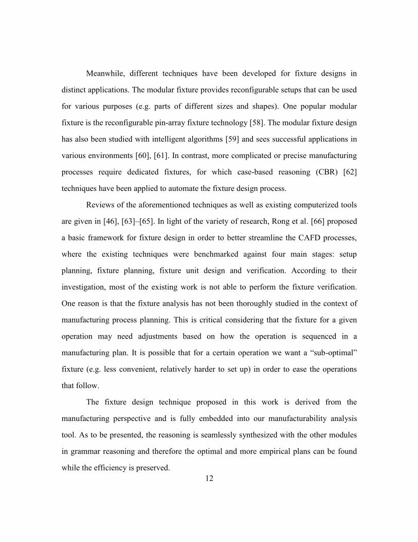
Figure 9: Grammar reasoning flowchart in AMFA.
Conversely, as seen in Figure 9, instead of finding a complete plan, the reasoning
may be terminated at different stop-points defined by different rule sets. Depending on
the functionality of each rule set, the reasoning can end when there are no rules applied in
a particular rule set (i.e. rule sets 2, 4 and 5), or when a particular termination rule is
triggered (i.e. rule set 3). For the first scenario, for example, the loop may stop if there is
no tooling operation identified in rule set 4 for a particular sub-volume. This situation
provides an insight to the user that the current sub-volume being machined is actually not
manufacturable with current available tools (defined in rule set 4). Since a foundry
capability is always mapped into different tooling rules, it is reasonable to conclude that
manufacturing this part is beyond the existing foundry capability. In this case, one has to
re-design the part to make it manufacturable (i.e. add or remove certain round edges), or
the complementary machines and tools need to be added to the foundry in order to cover

39
required operations. For the second scenario, for instance, the rules in rule set 3 define
several infeasible cases for tool entry face selection. If any of these rules is invoked, the
tool entry face selected in rule set 2 will be invalidated, and the search will be terminated
after this rule is triggered.
Therefore, depending on the geometry of the given part and the knowledge of the
manufacturability analysis built in the rules, a complete process described in Figure 9 will
either succeed with a feasible manufacturing plan, or find no plan. One should also be
aware that a complete loop from rule set 0 to 7 represents only one branch of the search
tree in Figure 2. The whole search process represented by the tree actually contains
numerous branches and therefore the search space grows exponentially with the
complexity of the geometry. Chapter 6 elaborates in detail how the size of the search
space is managed while the search effectiveness and efficiency are achieved.

40
Chapter 5: Fixture Design and Plan Evaluation
In manufacturing process planning, it is critical to ensure that the manufacturing
dependency between process planning and fixture design is assessed before a conclusion
regarding the optimality of a plan or the quality of a proposed fixture can be made. In this
chapter, we propose a concurrent reasoning for generating optimal fixture designs for a
manufacturing process plan [8]. It consists of two efforts. First, several grammar rules are
developed to encapsulate the knowledge that is critical to generate feasible fixture
mechanisms for a particular operation. A fixture mechanism provides a locating face and
one or two clamping faces depending on which clamping mechanism the fixture uses to
secure the work-piece in order to conduct current operation. The rules are included in rule
set 5 so that the reasoning is seamlessly synthesized with the other rules to perform
concurrent reasoning about the manufacturability of an input model.
In the second effort, the candidate operations with fixtures being generated in the
grammar reasoning are sent to an evaluation module, where each operation is measured
with respect to the manufacturing time, cost and fixture quality. For a given operation,
the time and cost needed can be estimated using both empirical and theoretical models
that are available in many engineering handbooks [78]–[80] and this implementation has
been reported separately in Van Blarigan’s work [81]. The fixture quality, however, is
uniquely defined in this work in order to provide a consistent and complete assessment of
a given fixture for an operation. The assessment is based on a collection of fixture design
guidelines that the author gathered from existing fixture design manuals [82]–[84]. As
confirmed from the experience in machine shop, these guidelines address common
concerns during the manufacturing processes (e.g.: stability, stress distribution,
accessibility, ease of implementation, etc.). The idea behind this is that by translating the

41
empirical and widely-followed fixture design guidelines to quantitative metrics, the
candidate fixture mechanisms defined in the grammar reasoning can be thoroughly
evaluated in a way closely resembling the actual manufacturing practice.
The work in this chapter sees major contributions in the following aspects:
1) We demonstrate an efficient and effective rule-based fixture design algorithm
as applied in the automated manufacturing process planning. For small one-off machine
shops, the plans are readily implementable; for modular and dedicated fixture unit
designs, the proposed fixture mechanisms provide optimal regions for setting up the
locating and clamping;
2) We identify the dependency between the fixture design and the manufacturing
process planning, and show via examples that the dependency is critical in defining
optimal and practical process plans;
3) We use manufacturing knowledge and experience to guide the generation of
optimal and practical fixture designs and process plans. This way, the multi-disciplinary
problems in the early fixture design phase are avoided.
5.1. DEFINING FIXTURE CANDIDATES WITH GRAPH GRAMMAR
A fixture design includes the selection of a locating face and one or several
clamping faces. The locating face refers to a face of the work-piece to be seated on
machine table, and the clamping faces are used to hold the work-piece firmly engaged
with the locating face during the machining. The fixture configurations considered in this
work are categorized into downward clamping (Figure 10a) and side clamping (Figure
10b) as suggested in [82]. The downward holding mechanism needs one clamping face
and the side clamping requires two faces for clamping.

42
Figure 10: Downward clamping and side clamping as applied on a work-piece.
Multiple rules are designed in rule set 5 with each defining a particular fixture
mechanism. Figure 11 is a screenshot of one rule that defines a downward clamping
mechanism in a vertical machining center (VMC). The rule is of the form L-to-R while
the left side of the rule specifies all the elements and conditions that need to be found and
satisfied in the seed graph in order to invoke the rule. The right side of the rule defines
necessary transformations on these elements that will be imposed by the rule. As shown
on the left, the rule needs to find three faces (denoted as “n0”, “n1”, “n2”) in the seed
graph that are parallel with each other (parallelism is imposed by arc “a0” and “a1” with
label “parallel”). One face (denoted as “n1”) must have a label “tool_entry”, which
indicates that this face has been chosen by rule set 3 as the tool entry face for current sub-
volume. The other two faces (denoted as “n0” and “n2”) do not have any label
constraints; therefore the rule will identify all pairs of accessible faces in the seed graph
that are parallel to the tool entry face. On the right side of the rule, one of the two faces
(in this case “n2”) is assigned a label “fixed”, meaning this face will be used as the
locating datum; and the other face “n0” is assigned labels “downward” and “clamp”,
saying that this face will be used as the downward clamping face. Meanwhile, a global
Face for clamping
Locating Face: sit on machine table
(a) Downward clamping: the locating face is
parallel to the clamping face
Locating Face: sit on machine table
(b) Side clamping: the locating face is
perpendicular to two parallel clamping faces
Faces for clamping

43
label “VMC” (on top of the right side of the rule) is assigned to the seed graph, informing
the later reasoning that a vertical machining center has been chosen for the current
operation. Note that the parallelism between the tool entry face “n1” and the locating
face “n2” ensures a VMC is invoked, and the parallelism between the clamping face
“n0” and the locating face “n2” specifies a downward clamping mechanism. As the rule
is applied on the seed graph, all possible downward-clamping fixture mechanisms in a
VMC are invoked for current operation.
Figure 11: Screenshot of a rule in rule set 5.
This rule defines a downward clamping fixture in a vertical machining
center.
Similarly, Figure 12 shows a rule that defines all possible side-clamping fixtures
in a VMC. There are additional rules in this rule set that define the two types of fixtures
in a HMC (horizontal machining center) and higher-axis machines, respectively. For
higher-axis machines, the faces for fixture are not necessarily parallel or orthogonal with
each other. In this case, the precise orientation of each fixture face is computed as well by

44
the rules. All knowledge and information captured in this rule set will be passed “on the
fly” to following rule sets in order to enable and facilitate further reasoning.
Figure 12: Screenshot of another rule in rule set 5.
This rule defines a side-clamping fixture in a vertical machining center.
5.2. EVALUATING FIXTURE CANDIDATES
After the candidate fixtures are generated, next task is to measure the quality of
each candidate against a set of consistent and meaningful metrics. According to Joshi
[82], a proper fixture design needs to be validated against several criteria. For locating, it
has to comply with the part’s dimensional requirements, and therefore machined faces are
preferred to set up the locating frame due to their relatively higher precision. Second, the
fixture needs to impose necessary constraints on the work-piece to ensure the part
stability during machining. Third, several common engineering concerns (strength, part
deflection and distortion, stress distribution, etc.) need to be addressed before a fixture
mechanism is actually mounted in a machine. As the fixture analysis overlaps with many
disciplines, it is hard to incorporate all issues in one fixture analysis module.
To tackle the problem, we view the fixture analysis directly from manufacturing
perspective. Despite the numerous issues in the early fixture design phase, a list of

45
guidelines that are used in the machine shop to facilitate the quick assessment of fixture
mechanisms have been generalized. As shown in Table 3, each guideline takes into
account several design criteria and is converted to a metric against which a candidate
fixture can be evaluated. Note that more design guidelines can be added to cover more
aspects of the fixture design.
Table 3: Fixture design guidelines and evaluation metrics.
Guidelines summarized from
[82]–[84] Design criteria
Evaluation metrics
(optimization strategy)
Available area for fixture faces
(locating face, clamping faces,
and tool entry face): larger is
better
Stress concentration,
clamping distortion, stability,
etc.
Face area (maximize)
Overlapping area between two
parallel fixture faces (e.g.
locating face and tool entry
face, two clamping faces, etc.):
larger is better
Clamping torque, stability,
cutting torque, clamping
distortion, work-piece
deflection, etc.
Overlapping area
between two faces
(maximize)
Distance between two parallel
fixture faces (e.g. locating face
and tool entry face, two
clamping faces, etc.): larger is
better
Stability, resultant torque due
to cutting forces, etc.
Distance between two
faces (maximize)
Spindle angle: smaller is better Tool deflection, ease of
fixture, etc.
Spindle angle
(minimize)
Face type: primitive features
(planar, cylindrical, etc.) are
better
Ease of fixture, stress
distribution, etc.
Face type (if not a
primitive feature,
assign penalty)

46
Next, a set of penalties are set up in Table 4, which represents extreme cases of
fixture design that need to be avoided. For example, Figure 13 gives a case where the
inaccessible penalty is assigned. Most penalties can be viewed as the consequences when
the metrics in Table 3 approach their extremes or singularities (i.e. the distance between
two faces is 0; the overlapping area of two faces reduces to 0; etc.). In addition, the Not-
primitive-penalty is assigned when the fixture face is not a primitive feature (i.e. planar
face, cylindrical face, circular face, etc.).
Table 4: Extreme cases that are penalized in fixture quality measurement.
Cases to penalize Instances Assigned penalty
Invalid operations or fixture Inaccessibility Penalty 10000
Need substantial change in
fixture mechanism
Coplanar penalty 1000
Tiny face penalty 1000
Require additional auxiliary
jigs
Not primitive penalty 100
Bad orientation penalty 100
Potential static or dynamic
mechanics problem
No overlapping area
penalty 10

47
Figure 13: A case where the inaccessibility penalty is assigned.
If we are to remove the pocket from top down, we do not want to use the top
shadowed face as the locating face as it will block the tool entry direction.
This case happens when the distance between the tool entry face and the
locating face reduces to 0 (i.e. they are coplanar).
The penalty assigned to each case has been carefully tuned based on the tests on
real parts to reflect the extent of infeasibility. The measurement is based on the
complexity and possibility of setting up a given fixture design. Cases with lower penalty
are easy to implement, but there may be some minor engineering concerns associated
with them. Cases with higher penalty are typically very hard, if not impossible, to set up.
The penalty levels are scaled by a factor of 10 such that each extreme case holds a
separate digit position. A side benefit is that by looking at the accumulated result after
evaluation, one can directly tell how many critical constraints the current design violates
and need to be resolved.
For each candidate fixture, a “fixture quality” synthesized from the evaluation
metrics is assigned. Since the quantity is treated as an objective to optimize in the search,
it needs to be monotonic [85]. That is, it should be monotonically increasing with a lower
value indicating a better fixture design. In order to achieve this, we take the reciprocals of
the metrics that are to be maximized and aggregate them with metrics to be minimized.
To compute the fixture quality, first it is initialized to zero. Then for every fixture design,
Undesired
locating face
Tool feed direction

48
Table 5 is traversed to identify which cells are applicable and need to be computed. All
the results will accumulate to form the final value of fixture quality. Note every cell in
the table is bounded by a corresponding penalty, which is used to capture the extreme
case.
Table 5: All computations needed to form the fixture quality.
Note that , and in the table are the reference spindle angle,
reference face area and reference length, which are used to normalize each
evaluation result to a unitless quantity.
Metric
Evaluation
Entry face Locating face Clamping face
1
Clamping
face 2
Overl-
apping
area
Locating
face
/overlapArea
No
Overlapping
Penalty
Clamping
face 1
/overlapArea
No
Overlapping
Penalty
/overlapArea
No
Overlapping
Penalty
Clamping
face 2
/overlapArea
No
Overlapping
Penalty
Dista-
nce
Locating
face
/dist
Inaccessibility
Penalty
Clamping
face 1
/dist
Coplanar Penalty
Clamping
face 2
/dist
Coplanar Penalty
Face area
Tiny Face
Penalty
/faceArea
Tiny Face Penalty
/faceArea
Tiny Face Penalty
/faceArea
Tiny Face
Penalty
Face type If not primitive:
Not primitive
penalty
If not primitive:
Not primitive
penalty
If not primitive:
Not primitive
penalty
If not primitive:
Not primitive
penalty
Spindle angle Bad orientation penalty

49
5.3. PLAN CONSOLIDATION
One assumption made in the reasoning is that each sub-volume can either be
machined in one operation or be non-machinable. However, a more realistic process plan
relies heavily on the type of operations and tools selected rather than the geometric
features, which are represented as sub-volumes in our case. In general, an actual
manufacturing process always starts with a roughing process in which the removal
volume is machined as much as possible. Such manufacturing knowledge is modeled in
our reasoning by consolidating the generated manufacturing plans into fewer steps that
resemble the roughing passes of realistic plans.
The idea is to integrate similar manufacturing operations in a plan into one unified
roughing pass. Given the current setup and tool, the reasoning detects all manufacturing
operations in the plan that can be implemented at one time and integrates them as one
step. To collapse the list of machining operations to only the number of unique part
setups in the process plan, we introduce a rule that operations requiring a re-fixture of the
part represent new setups, and cannot be combined with the previous operations. This is a
simple check to perform since in our algorithm the machine operations hold a Boolean
(i.e., true or false) for re-fixturing. Re-fixturing is set to true if any of the tool, the
machine and the fixture has changed, as doing such requires the re-orientation, re-
aligning and re-fixturing of the part. Therefore, re-fixturing will only ever be false if the
operation is in the same tool, the same machine and the same fixture as the previous
operation. If this is the case, the two operations can be combined.
An example of two operations that can be combined is shown in Figure 14. As
compared with plan I that requires two steps, the condensed plan II suggests only one
step to machine the pocket and the hole, which is more realistic from the human

50
perspective. It is also beneficial as it saves time and cost in manufacturing since we do
not need to re-fix the part when we continue machining the hole after the pocket.
Figure 14: Comparison of two plans with and without consolidation.
Initial raw stock (left) Final shape after machining (right)
Plan I - Step 1: drill the back hole from right
Plan I - Step 2: mill out the front pocket from left
Plan II - Step 1: mill out the pocket and hole from top

51
Chapter 6: Multi-objective Hierarchical Sorting based Best First Search
This chapter elaborates the search technique [8] that was developed to efficiently
find the near-optimal and empirical process plans among a huge space of solutions
defined by the grammar reasoning.
6.1. INTRODUCTION
CAMPP is a challenging task since it involves a large search space that contains
all possible process plans for an input part. One way to represent the space of plans is
with a tree structure (as depicted in Figure 15). The top of the tree is the initial state from
which the search process starts. The state can imply an input CAD model for machining
process planning, or a product assembly for assembly and disassembly planning. Every
level of the tree represents a step that specifies a particular manufacturing detail that will
later constitute a complete process plan. Multiple branches at each level represent
alternative options that are identified for a particular manufacturing detail. For example,
in machining process planning, one level can be designated to define an accessible region
in the solid model for the machining to start and every possible region in the CAD file
has its own branch at that level.

52
Figure 15: A tree structure of the search space in process planning.
The task is to find the complete and optimal process plans among the huge search
space. A complete process plan is essentially a path from the top of the tree to the bottom.
While uninformed search (such as Depth-first search) can be used to enumerate all
possible plans, an informed search (e.g. A*) can be used to more quickly find the optimal
plan.
To characterize the optimality of a plan, manufacturing time and cost are usually
used as evaluation metrics. Additional metrics may be added depending on which
problem domain within CAMPP one is solving. For assembly planning, the work load
imposed on labors needs to be carefully assessed. For the machining process planning
that the authors are studying [3], two more metrics are introduced: a unitless “fixture
quality” which evaluates the quality of fixture designs for a process plan against
manufacturing constraints, and a “remaining volume of material” factor which measures
how much material left to remove after every operation. With these criteria, the informed
search is a multi-objective optimization problem, where the preference over each
criterion needs to be articulated. Different optimization algorithms were summarized in
Initial state

53
[86], among which the weighted sum method is widely-used and effective to consolidate
multiple objectives into one:
∑
where is the i-th objective and is the weight associated with the objective. As
long as ’s are positive, minimizing U will give pareto-optimal solutions [87]. The
problem in CAMPP domain – as in many real-world applications – is that the objectives
are in different units, and some normalization technique has to be used in order to
consolidate these objectives. Second, there is usually no clear preferences over the
objectives from manufacturing that could tell the research how to set up the weights. As
the manufacturing knowledge is not well captured in the subjective setting of weights, the
optimal process plans found using a best first search technique are often not consistent
with the manufacturing practice, and are not readily implementable in a machine shop.
In this chapter, a hierarchical ordering based best first search algorithm is
proposed to solve the multi-objective CAMPP problems. The hierarchical method in
solving optimization problems defines a hierarchical order of the criteria, and the criteria
on top have the authority to strongly affect the performance of other criteria [88]. Based
on the hierarchy, the objectives are solved one at a time:
where i represents the position of corresponding objective in the preference list. As an
extension of Stackelberg strategy [89], the hierarchical optimization has been widely
studied in various areas [90], [91], and the assessment of its performance is available in
[92]–[94].
In this work, we establish the hierarchy of the evaluation criteria, and the
promising branch of the tree that the search algorithm chooses is defined by the criteria

54
hierarchically. We will compare the performance of the hierarchical search in
manufacturing planning with A* search through examples. The observation from this
work is that by incorporating the manufacturing knowledge and practice into the
hierarchy of the objectives, the new search is able to find optimal yet practical solutions
in near-linear time.
Three major contributions are summarized from this work:
1) We demonstrate an effective and efficient hierarchical ordering based best first
search algorithm as applied in the automated manufacturing process planning.
2) We show via examples that the search effectiveness can be greatly improved
by customizing the search with particular engineering knowledge.
3) We demonstrate that the multi-objective optimization problem can be
effectively solved with hierarchical ordering of evaluation metrics. The dependency of
the optimality of solutions on the weight associated with each metric is removed.
The chapter is organized as follows. Next section talks about the hierarchy of four
evaluation metrics and the sorting strategy used in the search. Then the search efficiency
and practicality are discussed in detail. The characteristics of the search are validated
through two case studies and observations from the results. The chapter ends with a
summary of the algorithm.
6.2. SEARCH HIERARCHY AND SORTING STRATEGY
Four metrics are set up to evaluate the optimality of a manufacturing process plan:
the manufacturing time, the manufacturing cost, the fixture quality and the remaining
volume under current operation. While the search is traversing down the tree, we want
the accumulating plan to consume as little time and cost as possible. For the fixture
penalty, it is converted from a set of fixture design guidelines collected from engineering

55
handbook and machine shop experience. It gives a comprehensive assessment of the
fixture designs proposed by our manufacturing process planning tool.
The remaining volume under current operation is treated as a heuristic that leads
the search quickly to the optimal solution. One goal during the search is to reduce the
remaining volume as much as possible after every step. It is a reflection of the real
machining practice in which we want to remove as much material as possible before we
have to change the setup to initiate next operation. For example, to start the machining of
the part in Figure 16, two alternative plans are defined in the search space as shown in
Figure 14. Given the raw stock, plan I suggests drilling the holes from right as the first
step and then milling the pocket from left as a second step. Plan II suggests creating the
pocket and the hole from top in one step. While both options are implementable, plan II is
better as it saves time and cost by removing more material within the initial setup. This
option also puts the plan closer to the final solution as less material (in this case no
material) is left to remove as compared to plan I.
Figure 16: An illustrative part.
Figure 17 shows the search queue structure and the evaluation strategy based on
the hierarchical sorting of metrics. The hierarchy of the metrics is set up as follows: the

56
options in the search space are sorted by the remaining volume, and then by the fixture
quality, followed by the machining time, and last by the machining cost. Sorting on
remaining volume first guarantees a quick convergence of the search to complete
machining process plans. For candidates with the same remaining volume, they are next
ordered by fixture quality – thus putting a priority on fixturing, which is a significant
chore in machining. One does not want to generate any plan that later is shown
impractical because the fixtures are too complicated – if not impossible – to create within
machine shops. After this, the time and cost are evaluated. The time goes first because –
given a machine shop – the facilities, labor, and overhead are based on this. Shorter
machining time directly lowers the cost. While there are often negotiations over the cost
with clients, the time is a more sensitive factor to manufacturing engineers. With the
manufacturing background knowledge embedded into the hierarchy of the metrics and
sorting strategy, the purpose is that the search is better informed to find optimal yet
practical plans.
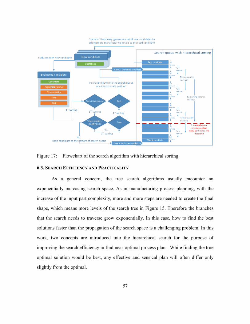
57
Figure 17: Flowchart of the search algorithm with hierarchical sorting.
6.3. SEARCH EFFICIENCY AND PRACTICALITY
As a general concern, the tree search algorithms usually encounter an
exponentially increasing search space. As in manufacturing process planning, with the
increase of the input part complexity, more and more steps are needed to create the final
shape, which means more levels of the search tree in Figure 15. Therefore the branches
that the search needs to traverse grow exponentially. In this case, how to find the best
solutions faster than the propagation of the search space is a challenging problem. In this
work, two concepts are introduced into the hierarchical search for the purpose of
improving the search efficiency in find near-optimal process plans. While finding the true
optimal solution would be best, any effective and sensical plan will often differ only
slightly from the optimal.

58
6.3.1. List Reordering Based on Limits on Objectives
A limit is used to deter the search from considering states that have one of the
four objectives above a specific cutoff value. This introduces practical engineering
heuristic into the otherwise naïve search algorithm. For example, a limit is set for the
fixture quality. Referring to the additional fixture quality check in Figure 17, if the fixture
quality is larger than the cutoff value, the search will immediately move the candidate to
the bottom of the search queue regardless of where the hierarchical sorting places the
candidate (which would be with others that have identical remaining volume). This
makes the process more efficient and leads to more practical results since these highly
unlikely plans are not expanded in the tree search at the time of others with like volume.
This fixture cutoff is prescribed to a value corresponding to a likely infeasible fixture.
The computational resources saved by the cutoff are thus relocated to expanding
other branches in the search space. The concept is also extended to the third and fourth
heuristics: time and cost, but there appears to be little impact on the results or speed.
Naturally, it does not make sense to apply such a strategy on the first heuristic (remaining
volume) since solutions of high value are already at the bottom of the search queue. This
approach should be considered in any hierarchical search in order to ensure that time is
not wasted on candidates that – while having good values for their first objective – have
very poor values for the other objectives.
6.3.2. Search Queue Truncation
Another modification is to place a limit on the maximum length of the search
queue. As shown in Figure 17, any candidates that are outside of the maximum queue are
discarded. This has the obvious effect of making the search more efficient while
preventing problems with handling more solutions than is budgeted. For this particular

59
problem, we show via examples that the optimality of the solutions is not affected by the
imposed incompleteness of the search space for two reasons.
First, in hierarchical search, the candidates at the bottom of the queue are those
with more remaining volume, larger fixture quality, longer machining time, and more
cost as well as those exceeding aforementioned cutoffs. These non-optimal states do not
contribute to the generation of optimal or best plans as measured by the metrics.
Second, in CAMPP problem, a complete process plan involves a diverse set of
decisions, such as accessible regions to start an operation, feasible feed directions for the
tool, available machines to use, available tools to use on each machine, and the fixtures to
secure the part during the operation. So, it requires at least 5 levels of the search tree to
fully specify a given operation with each decision having a branching factor, b, that is
adequately large ( ). Therefore, the first complete operation may have over 3000
options ( ). As such, truncating seemingly poor partial states is a necessary
process. It is theorized that for the problem at hand, there is a strong consistency between
local decisions and their impact on complete plans. There does not appear to be the
situation in manufacturing planning that sometimes inflicts other path-planning problems,
such as in traversing a maze where “going south first” may be the best way to “go north
in the end”.

60
6.4. CASE STUDIES
The hierarchical search algorithm is characterized in terms of optimality,
practicality and efficiency through two case studies and observations.
6.4.1. Example 1
Consider the part shown in Figure 18. The optimal process plans found by
hierarchical search is compared with the results from an A* search algorithm using
weighted sum method to consolidate the evaluation metrics. To limit the memory use and
maintain the efficiency, the search queue length is limited to 600.
Figure 18: Example part 1.
Table 6: Comparison between hierarchical search and A* search for example 1.
Maximal queue size is set to 600.
Experiment Total solutions
found
Quality of optimal plan
Mfg. time (min) Mfg. cost ($) Fixture quality
1 Hierarchical
search 300 35.86 23.79 0.2763
2 A* 300 71.42 46.32 7149.93
3 A* 1000 74.63 48.68 5200.35
In Table 6, the optimal plans are assessed in terms of time, cost and fixture
quality. We can see among the first 300 plans found by the two algorithms, the
hierarchical search has a much better optimal solution. In fact, in the third experiment, we

61
waited for the A* search to find 1000 solutions before an optimal plan was filtered. In
this experiment, A* reported a plan with smaller fixture quality but slightly worse time
and cost as compared to the last experiment. Due to the weights of the metrics, this plan
was considered better than the other one from A*. However, it is still far behind the first
plan from hierarchical search. These comparisons indicate that in solving CAMPP
problems, the hierarchical search converges much faster to the optimal plans than the
weighted-sum A* search.

62
Figure 19: Comparison of two plans for example 1.
Plan I from hierarchical search and Plan II from A* with 1000 solutions.
The arrow indicates the feed direction. For the fixture mechanism, the
bottom face is the face for locating the part on the machine table, and the
side two faces are the faces for clamping.
Figure 19 shows the plans from hierarchical search and A* with 1000 solutions,
respectively. The second one is not optimal as it requires unnecessary setup changes (step
2 and 3) and an uncomfortable feed direction (step 3), which lead to more time and cost
and penalized fixture quality.
Initial raw stock
(left) Fixture mechanism
(middle) Final shape after
machining (right) Plan I - Step 1: mill out pockets and slots from top
Plan II - Step 1: flip part over, drill holes from bottom
Plan II - Step 2: flip part over, mill side slot from top
Plan II - Step 3: mill middle pockets and slots from side

63
6.4.2. Example 2
For the second example show in Figure 20, experiments with the same settings as
in example 1 were conducted and the results are given in Table 7. Again the hierarchical
search is able to find a much better plan. Figure 21 shows the plan details step by step.
Figure 20: Example part 2.
Table 7: Comparison between hierarchical search and A* search for example 2.
Maximal queue size is set to 600.
Experiment Total solutions
found
Quality of optimal plan
Mfg. time (min) Mfg. cost ($) Fixture quality
1 Hierarchical
search 300 67.89 45.13 10.96
2 A* 300 123.75 82.05 24285.78
3 A* 1000 139.75 92.72 22275.77
Front view Top view

64
Figure 21: The optimal plan generated by hierarchical search for example 2.
6.4.3. Discussion
More experiments were implemented to validate our algorithm. Due to the space
limitation, the results are not presented. This section mainly characterizes the search
efficiency based on the analysis of the test results.
Figure 22 shows a plot of the computation time to find the first optimal solution
against the complexity of the input solid model based on the results of the experiments.
The complexity is measured by the number of sub-volumes that need to be removed from
a bounding box in order to create the final shape.
Initial raw stock
(left) Fixture mechanism
(middle) Final shape after
machining (right)
Step 1: mill out features from top
Step 2: flip part over, mill out features from bottom
Step 3: remove left fillet
Step 4: remove right fillet

65
An interesting observation is that as opposed to the exponentially increasing
search space, the hierarchical search is able to find the first optimal and practical solution
in near-linear time. The reason is that the hierarchical search always specifies a
“promising” direction at every level of the tree for the best first search to go. The
computation time is only dictated by the length of the complete process plan from the top
to the bottom of the tree, which is proportional to the number of sub-volumes to remove.
Therefore the computation time is linear rather than exponential.
Figure 22: The plot of computational time versus part complexity.
It shows the linear trend of the computation time for hierarchical search to
find the first optimal solution with the complexity of the part.
For the part shown in Figure 16, an exhaustive search was performed to generate
the complete search space. Figure 23 summarizes the exhaustive search process. Within a
very short computation time all 96 solutions were generated for this simple part. All the
solutions were manually verified in order to ensure the completeness of the search space.
Among all the solutions, the exhaustive search gave the same best plan shown as Plan II
in Figure 14 that was previously found by our hierarchical sorting based search. As
opposed to 127 solutions (shown in Figure 23) that had been tested before the best one
was reported in the exhaustive search, our new algorithm is more efficient since the first
solution it converged to was the best one.
y = 13.491x
R² = 0.9953
0
50
100
150
200
250
300
0 5 10 15 20
Com
pu
tati
on
tim
e
Number of sub-volumes to remove

66
Figure 23: Summary of the exhaustive search for the part in Figure 16.
6.5. SUMMARY
In this chapter we present a multi-objective hierarchical sorting based best first
search technique and successfully apply it in solving manufacturing process planning
problems. The hierarchy of the objectives is set up in accordance with the manufacturing
knowledge and preferences. The cutoffs for fixture, time and cost are used to adjust the
search queue in order to capture the impractical manufacturing decisions. The search is
educated by the manufacturing knowledge such that it is able to find the optimal and
implementable process plans in near-linear time.
To extend the technique to other areas of CAMPP (like assembly and disassembly
process planning), similar strategies as mentioned in the chapter can be used. It is
suggested that an initial detailed study of the problem domain would be beneficial in
encapsulating the underlying knowledge. Such domain-specific knowledge should not
only be used to define evaluation metrics but also used to tailor the sorting strategy –
even if such a strategy is as aggressive as the hierarchical sorting shown here – in order to
yield practical results.

67
Chapter 7: Case Studies and Discussions
Several examples are provided in this chapter to validate our algorithm in
manufacturability analysis. Each of the examples showcases different aspect of our work.
The next three sections are tilted with the part name followed by the aspect that we are
highlighting. Section 7.4 discusses the non-manufacturability reasoning in our approach
and section 7.5 itemizes the characteristics of the computerized tools built on our
approach.
7.1. RADIOBOX: DYNAMIC ALLOCATION OF FACES FOR OPTIMAL FIXTURE DESIGN
The first part presented – refer to as the “Radio box” – is a vehicle component
design from our research partner (Figure 24). It is interesting in its complex profile and
intersecting features. In this case, the actual manufacturing sequence dictates the fixture
design for each operation since most planar faces that are preferred for fixture are
actually created by intermediate steps and are subject to subsequent tooling as well.
Figure 24: CAD model of the “Radio box”.
Table 8 shows an optimal plan with fixtures for each step generated using our
approach. The first column describes each step briefly, and the second column is the
initial work-piece that each step starts to machine. The third column shows the faces that
a) Up-front view b) Back view

68
are used to set up the fixture mechanism at each step and the fourth column is the part
created after every step.
In this plan, step 2 requires an intermediate face, which is created in step 1, as the
locating datum to set up the work-piece. Step 4 is necessary to machine the bottom left
chamfer and the left side wall as these features are partially used for clamping in step 3
and therefore are not available for the tool to enter at that step. The dynamic allocation of
faces that are either preserved in the final part or are created but removed during
intermediate steps for optimal fixture design is a unique feature of our algorithm.

69
Table 8: An optimal manufacturing plan with fixtures for Radio box.
The cutoff value for fixture quality is set to 1000. Cutoff value for the
number of optimal solutions is set to 600. Maximal queue size is set to 300.
Total run time is 313.936s.
Step
description Initial work-piece2 Fixture mechanism3 Final work-piece
1: side
clamping in
Vertical
milling center,
use End mill,
feed along –z
direction
2. side
clamping in
Vertical
milling center,
use End mill,
feed along x
direction
3. side
clamping in
Vertical
milling center,
use End mill,
feed along –z
direction
2 For all the cases, the initial work-piece at step 1 is the bounding box, and after that the final work-piece
at a previous step is served as the initial work-piece of the next step. 3 Refer to Figure 10 for the definition of the face configurations. For side clamping, the bottom face is the
locating face and the two side faces are the clamping faces. The faces shown here are only used to indicate
the orientations of the actual fixturing faces on the work-piece. While the exact fixturing areas projected on
each face are identified automatically in the reasoning, not all are explicitly shown due to the tedious
visualization process.
x y
z
z y
x
x
z
y

70
Table 8 (continued): An optimal manufacturing plan with fixtures for Radio box.
The cutoff value for fixture quality is set to 1000. Cutoff value for
the number of optimal solutions is set to 600. Maximal queue size
is set to 300. Total run time is 313.936s.
Step
description Initial work-piece Fixture mechanism Final work-piece
4. side
clamping in
Vertical
milling center,
use End mill,
feed along -x
direction
Although Table 8 shows only one optimal plan, our reasoning actually suggests
multiple pareto-optimal plans with each varying slightly in terms of time, cost and fixture
quality. The runtime to generate 600 optimal plans is about 5 minutes4. The total
manufacturing time is estimated to 41.68 min.
7.2. PART II: DEPENDENCY BETWEEN FIXTURE DESIGN AND MANUFACTURING
PROCESS PLANNING
The part in Figure 25 is a benchmarking problem found in the feature-recognition
research community. It is of a simple prismatic shape, but is not that intuitive to
manufacture. The slots on top are intersecting and the islands at four corners are of
different sizes, which require tool changes during the process planning.
4 All experiments were implemented on a desktop computer with Intel 3.4 GHz processor and 16 GB of
memory.
z
y
x

71
Figure 25: CAD model of part 2.
An optimal plan from the reasoning as shown in Table 9 suggests that the initial
stock needs to be set up with bottom slot facing upward such that the slot is created first.
Next, the work-piece is flipped over so that the tools can create the features on top. Note
that if the fixture design is not considered, the bottom slot is an isolated feature that can
be created at any step of a manufacturing plan. Nevertheless, if we incorporate fixture
design into the reasoning, it is better to machine the slot first. Considering that all other
features reside on top, it is more reasonable to first locate the bottom slot using the un-
machined top face as it gives larger locating area as well as preventing the top features
from being contaminated by fixtures that may be required for machining the slot in later
steps.
An implementation of the proposed plan in a machine shop is also shown in Table
9. The experiment justifies the practicality of the proposed plan in one-off machine
shops.

72
Table 9: An optimal manufacturing plan with fixtures for part II.
The cutoff value for fixture quality is set to 1000. Cutoff value for the
number of optimal solutions is set to 200. Maximal queue size is set to 300.
Total run time is 447.864s.
Step
description Initial work-piece Fixture mechanism Final work-piece
1: side
clamping in
Vertical
milling
center, use
End mill,
feed along z
direction
Results from AMFA
Implementation in machine shop: side clamping setup in VMC
y x
z
z
x
y z
y
x
z
x
y

73
Table 9 (continued): An optimal manufacturing plan with fixtures for part II.
The cutoff value for fixture quality is set to 1000. Cutoff value
for the number of optimal solutions is set to 200. Maximal
queue size is set to 300. Total run time is 447.864s.
Step
description Initial work-piece Fixture mechanism Final work-piece
2. side
clamping in
Vertical
milling
center, use
End mill,
feed along –
z direction
Results from AMFA
Implementation in machine shop: side clamping setup in VMC
Table 10 gives a comparison between the AMFA-suggested tooling parameters
and the actual parameters used at each step during the real implementation. Note the
actual parameters are less than – if not equal to – the suggested values. The reason is that
the machine shop does not have a complete tool library as assumed in AMFA. In
addition, due to the limitation of the manually operated machines, it is always safer to
choose a relatively smaller tool to do the required machining.
z
x
y
z
x
y
z
x
y
z x
y

74
Table 10: Comparison between the manufacturing parameters suggested by the
reasoning and the actual choices in the machine shop for part II5.
No. Operation Tooling
parameter
Suggested from
AMFA
Actual choice in
machine shop
1 Create bottom slot
Tool diameter 1 3/4 = 0.75
Depth of cut 0.15 0.15
Feed rate 0.086 0.05
2
Create left slot
Tool diameter 0.75 3/4 = 0.75
Depth of cut 0.55 0.55
Feed rate 0.086 0.05
Create top slot
Tool diameter 0.75 3/4 = 0.75
Depth of cut 0.15 0.15
Feed rate 0.086 0.05
Create intersecting
holes
Tool diameter 0.4 25/64 = 0.390625
Depth of cut 0.3 0.3
Feed rate 0.051 0.03
Create secondary
slot
Tool diameter 0.32 5/16 = 0.3125
Depth of cut 0.15 0.15
Feed rate 0.036 0.03
Create up-right and
bottom-right pocket
Tool diameter 0.375 3/8 = 0.375
Depth of cut 0.3 0.3
Feed rate 0.036 0.03
Create up-left and
bottom-left holes
Tool diameter 0.24 7/32 = 0.21875
Depth of cut 0.2 0.2
Feed rate 0.03 0.03
5 All length parameters are in inch, and the feed rate is in inch per second.

75
7.3. STABILIZER: SYNTHESIZED REASONING APPLIED IN MANUFACTURING
COMPLICATED FEATURES
The third part is a simplified vehicle stabilizer design from our research partner.
As shown in Figure 26, the part has a contour groove around a center rib, which is not
that intuitive to machine. In fact, the groove needs several steps to finish, and the
complexity of the fixture design at each step depends highly on how the operations are
sequenced. Further, as the feed direction for the left hole and right through pocket does
not coincide with any of the feasible feed directions for the groove, how to arrange the
operations for minimal time and cost is challenging. Because of these problems, a
synthesized manufacturability analysis as implemented in our reasoning is necessary.
Figure 26: CAD model of the stabilizer.
For this part, the reasoning successfully generated several optimal plans in about
5.5 minutes. One of them is given in Table 11.

76
Table 11: An optimal manufacturing plan with fixtures for the stabilizer.
The cutoff value for fixture quality is set to 1000. Maximal queue size is set
to 300. Total run time is 325.674 s.
Step
description Initial work-piece Fixture mechanism Final work-piece
1: side
clamping
in Vertical
milling
center, use
End mill,
feed along
–y
direction
Results from AMFA
Implementation in machine shop: side clamping in VMC
2. side
clamping
in Vertical
milling
center, use
End mill,
feed along
y direction
Results from AMFA
Implementation in machine shop: side clamping in VMC
z x
y
z
x
y
z
x
y
z
x y
z
x y
z
x y

77
Table 11(continued): An optimal manufacturing plan with fixtures for the stabilizer.
The cutoff value for fixture quality is set to 1000. Maximal
queue size is set to 300. Total run time is 325.674 s.
Step
description Initial work-piece Fixture mechanism Final work-piece
3. side
clamping in
Vertical
milling
center, use
End mill,
feed along -
z direction
Results from AMFA
Implementation in machine shop: side clamping in VMC
Following the suggested plans, we were able to replicate the stabilizer in three
steps in the machine shop rather than the high-tech manufacturing facility in the
automobile industry where the part is usually created. Table 12 compares the suggested
tooling parameters with the actual choices, where most of the parameters are the same.
For step 3, the difference in machining the pocket is due to the slight inconsistency of
tool libraries used in the two environments. For the drilling in step 3, we intentionally
used a smaller tool in the consideration of a future reaming operation.
y
x
z
Final part
z
x
y
z y
x
z
y
x
z
y
x

78
Table 12: Comparison between the manufacturing parameters suggested by the
reasoning and the actual choices in the machine shop for the stabilizer.
No. Operation Tooling
parameter
Suggested from
AMFA
Actual choice in
machine shop
1 Create top slot
Tool diameter 0.5 0.5
Depth of cut 0.375 0.375
Feed rate 0.051 0.03
2
Create bottom
slot
Tool diameter 0.5 0.5
Depth of cut 0.375 0.375
Feed rate 0.051 0.03
Create left slot
Tool diameter 0.5 0.5
Depth of cut 0.25 0.25
Feed rate 0.051 0.03
Create right slot
Tool diameter 0.5 0.5
Depth of cut 0.25 0.25
Feed rate 0.051 0.03
3
Create left
Tool diameter 0.45 7/16 = 0.4375
Depth of cut 1 1
Feed rate 0.051 0.03
Create right
hole
Tool diameter 0.5 7/16 = 0.4375
Depth of cut 0.25 0.25
Feed rate 0.051 0.03

79
7.4. NON-MANUFACTURABILITY ANALYSIS
The non-manufacturability of a given part is due to two constraints. One is the
production facility limitation and the other is the design flaw of the CAD model. The
non-manufacturability analysis in the grammar reasoning is implemented by topological,
rather than parametric reasoning through the recognition and application of rules. At this
stage, we intentionally relax the parametric constraints imposed by the foundry
capability. One reason is that these constraints, such as the lack of appropriate tool sizes,
can always be solved by importing required tools into the foundry. Thus, no redesign
feedback for the designers is needed. However, the design flaws detected by the
reasoning usually relate to the topological defects in the given part. The underlying logic
behind this reasoning is that if a part is topologically not manufacturable because of 1)
inaccessible regions (for example, the inner sharp corners of the part in Figure 27a) or 2)
unrecognized or invalid geometric elements (for example, an edge with more than two
vertices), then this part would always be recognized as non-manufacturable unless the
required redesign modifications are made by the users.
Consider the part in Figure 27a. It is not manufacturable due to an inaccessible
sharp edge from any tool feed direction. From the analysis report shown in Figure 27c we
see that the reasoning asserts that no manufacturing plan can be found for this part.
Additionally, the user is informed that all the inner sharp edges should be removed before
any machining operation can start. This example shows how our reasoning communicates
with the user in terms of design improvements.

80
Figure 27: (a) A non-manufacturable part due to design flaws, (b) the machined part
simulated in FeatureCAM, and (c) the manufacturability analysis result
generated in AMFA.
For comparison, this part was also processed in FeatureCAM [10] and the
proposed manufacturing plan is shown in Figure 28. In this plan, several stages of
roughing and finishing passes are used to remove the negative cuboid. However,
considering the manufacturing precision that the tools can achieve, the sharp edges would
never be created exactly as designed. Figure 27b shows the amount of residual material
that is left over after the plan is implemented. These areas are exactly where the non-
manufacturable sharp edges locate. Rather than attempting to tackle the bad geometries
by the ineffective employment of foundry capability, our approach is able to return
redesign suggestions directly to the end-user in a much earlier phase, which is critical to
ensure the efficiency and effectiveness of modern product design.
Figure 28: A sample manufacturing plan generated in FeatureCAM.

81
7.5. CHARACTERISTICS OF IMPLEMENTATION AND DEPLOYMENT
The geometric and grammar reasoning demonstrated in Part I serve as the
foundation based on which multiple computerized tools can be developed. Figure 29
shows one web-based GUI that was developed to visualize the functionalities of AMFA.
Figure 29: A sample AMFA GUI.
The key characteristics of the tool are summarized as follows:
The tool is customizable based on available resources of a particular foundry. The
manufacturing capability can be extended from the widely used traditional
operations to the non-traditional and new-born manufacturing techniques. We
have demonstrated the aptitude of the tool for reasoning about various machine
libraries provided by our research partners.
The tool is capable of analyzing complex geometries, including feature
interactions. The complex regions are decomposed into simple and prismatic
machining features (sub-volumes) for the rules to reason about.

82
The tool allows the user to step through individual steps of a proposed plan and
see the staging models, i.e., the geometry that is created after every step of the
plan. Since each step removes one sub-volume in the compound negative solid,
the remaining negative solid constitutes the staging model. This feature allows the
easy validation of every plan, and provides a concrete means for designers to
communicate with manufacturing engineers about the feasibility of the suggested
plans.

83
Chapter 8: Part I Summary
In this part, an efficient and effective approach to automated manufacturing
process planning is demonstrated for any solid model that requires non-turning
operations. The approach is split into the geometric reasoning and the grammar
reasoning. The geometric reasoning is a separate work from the dissertation and is
developed to decompose the solid model into machinable sub-volumes and to convert the
resulting sub-volumes to a graph representation. The grammar reasoning is realized using
the specially designed seed lexicon and graph grammar based rules. The seed lexicon
stores all geometric elements and their topological relations of a solid model through
nodes, arcs, hyperarcs and labels. The grammar rules are deployed in a particular
sequence to invoke all feasible sequences of machining operations that are necessary to
create the input CAD model. Each operation is detailed with the amount of material to
remove, the tool and machine specs, the tooling parameters, and the fixture mechanism.
After the candidate manufacturing plans are generated by the grammar rules, they are
evaluated in terms of time, cost and fixture quality, and a hierarchical sorting based
search algorithm is developed to find the optimal and practical plans efficiently.
This work highlights the important interaction and dependency between the
fixture design and the manufacturing process planning. Depending on how the part is
machined, the fixture needs to be designed in accordance with the operation at each step
in order to achieve the optimality as well as the practicality of a proposed plan.
For the fixture design, instead of considering it from a pure design perspective
where specific subjects are investigating and their influences on the fixture design are
assessed, this work first invokes all feasible fixtures with several simple rules. Then the
knowledge gathered from manufacturing practice is used to dictates the selection of
84
optimal fixtures. Through multiple case studies, we see that the strategy enables an
concurrent and effective fixture design algorithm in the context of manufacturing
planning.
A hierarchical sorting based best-first search algorithm is also introduced in this
work. While the motive is to incorporate intuitive manufacturing background knowledge
to the otherwise naïve search algorithm, the same idea can be applied in other research
areas. For example, in assembly planning or robot path planning where the space of
solutions expands with the complexity of the problem, the a priori knowledge can be used
to better inform the search in order to achieve a much quicker convergence to optimal
and practical solutions.

85
PART II: AUTOMATED REASONING FOR DEFINING TURNING
OPERATIONS FOR MILL-TURN PARTS
To automate the manufacturing planning for the hybrid machining processes (e.g.
mill-turn machining), a smart system is developed which defines the detailed
manufacturing plans that are optimized in time, cost, fixture quality and tolerance
satisfaction for any input CAD model. The system includes two parts. The first is a tool
known as AMFA (Automated Manufacturability Feedback Analysis), which is introduced
in Part I of this dissertation and is capable of reasoning about the non-turning
manufacturing processes and generating user-preferred plans based on these operations.
This software has been tested thoroughly and results along with the detailed description
are reported in [3], [7], [8], [95]. One limitation of AMFA is that it cannot handle
complex parts which require hybrid manufacturing processes. For example, consider a
part with both turnable and non-turnable features. While the non-turnable features are, in
principle, manufacturable in a milling center, the turnable features are more complicated
to be machined via milling and require extra turning operations. In this case, how to
arrange the manufacturing sequence as a whole for achieving the lowest time and cost
becomes a question. Moreover, the fact that the turnable and non-turnable features are in
most cases interacting makes the reasoning more challenging.
To resolve this issue, the research in the second phase [6], [9] is presented in this
part, which aims to automate the reasoning for defining the lathe operations for complex
geometries. It has a similar two-phase structure as AMFA: the geometric reasoning and
the grammar reasoning. The geometric reasoning is a separate work done by Eftekharian,
and is introduced in chapter 9. From a given CAD model, we extract both its bounding
cylinder and the as-lathed axisymmetric model. Since the as-lathed model serves as the
intermediate work-piece after all turning operations, the turnable volume can be

86
generated by subtracting the as-lathed model from the bounding cylinder. Meanwhile, the
non-turnable volume can be extracted by subtracting the final part from the as-lathed
model. After that, the turnable and non-turnable volumes are sent to a volume
decomposition algorithm [5] to generate the isolated machining features. Features
generated from the non-turnable volume are fed into AMFA to generate the optimal
manufacturing plans in terms of time, cost and fixture quality.
To automate the process planning for the turnable features, first these features
along with their tolerance specifications are represented by a tolerance graph. This graph
then serves as the seed on which the grammar reasoning performs analysis in order to
study feasible turning sequences against the tolerance specifications. The reasoning is
based on the direct analysis of the knowledge conveyed by the design tolerances. The
output from the grammar reasoning is the feasible turning plan for creating all turnable
features. This plan is validated using a separate tolerance analysis module to show its
effectiveness in satisfying the tolerance requirements.
By integrating both parts of the research, the final goal of this work is to propose
a novel manufacturability analysis tool that is able to quickly inform the users (e.g.
designers or manufacturing engineers) of the optimal plans in terms of time, cost, fixture
quality and tolerance satisfaction for a given solid model that requires hybrid
manufacturing processes.
This part is organized as follows. In chapter 9 the algorithm developed by
Eftekharian to automatically separate the turnable and non-turnable features is
introduced. It also converts the turnable features to a graph representation for the
grammar reasoning to work on. Chapter 10 illustrates how the tolerance specifications
dictate the setup design for turning operations. Beyond that, chapter 11 presents the
grammar rule based reasoning to generate turning plans for the turnable features via an

87
illustrative case study. Another example and discussions are provided in chapter 12,
which is followed by the validation of the suggested turning sequences (chapter 13) and
the conclusion (chapter 14).

88
Chapter 9: Geometric Reasoning
This chapter explains the geometric reasoning work done by Eftekharian, which
extracts the turnable features from a mill-turn part and converts them to a graph
representation for the grammar reasoning to work on. While the author of this dissertation
did not develop the algorithm, the author led the integration of this part with the grammar
reasoning and the combined work has been published in [6], [9]. It is incorporated in the
dissertation for a better understanding of the major work that follows.
The features in a mill-turn part can be categorized into two classes, turnable and
non-turnable. One challenge in reasoning about the manufacturing is to correctly identify
and successfully isolate the two types of features in order to assign feasible machining
operations to each. Figure 30 shows a sample model with some non-turnable features that
are not machinable in a typical turning operation.
Figure 30: A sample part with non-turnable features.
To isolate these features, the reasoning starts by generating the accurate as-lathed
model. The as-lathed model is the intermediate work-piece that is created after all the
turning operations on the bounding cylinder or the initial raw stock. The as-lathed model
can be viewed as the result of revolving a two-dimensional axisymmetric silhouette
around the rotational axis. Therefore, the problem of defining the as-lathed model can be

89
formulated as finding the rotational axis of a mill-turn part and then generating the de-
featured silhouette.
One approach to generate the as-lathed model that is largely used in the past
literature is to revolve the original solid around a rotational axis defined by the designer
in order to fill in all the non-turnable features. This is not desirable in computational
geometry as the general sweeping operations (in which revolving is a special case) are
computationally expensive for 3D shapes in almost all solid modeling kernels. As a
result, this procedure is particularly slow and potentially inaccurate for complex parts
with blended features.
In this chapter, a simpler and efficient method is proposed. It starts by
automatically finding the dominant rotational axis from the CAD model. Next, it samples
a set of non-uniform longitudinal cross sections of the original solid passing through the
dominant rotational axis. In order to perform each sampling, a planar cutting face is
needed. This plane can be created by a point and a normal vector, where the point can be
any point along the rotational axis, and the normal is a unit vector perpendicular to the
rotational axis. These planes are used to cut the model to generate many cross sections of
the geometry. The revolving silhouette is then created by uniting all these cross sections,
and the as-lathed model is formed by sweeping the silhouette for a full circle. The
complete process is explained in detail in the following sections.
9.1. DETECTING THE DOMINANT ROTATIONAL AXIS
In order to identify the dominant rotational axis, the algorithm first recognizes all
the curved edges in the boundary representation of the original part by collecting their
center points, radii and axial normal vectors (Figure 31). A curved edge refers to any

90
edge with a constant radius, such as a full-circular edge, a semi-circular edge, or a fillet
edge. For every curved edge, two parameters are defined. The first is the number of the
other curved edges N that are co-axial with the current edge. The other is the radius of the
edge, R. The dominant rotational axis of the part is defined as the axis of the edge with
the maximum product of the two parameters (N R).
This sorting method guarantees that the dominant rotational axis is shared by the
most curved edges. This is consistent with the real turning practice: when a raw
cylindrical stock is initially set up in a turning machine, it is desirable to turn as many
features as possible under the initial setup. If certain features are off center from the
current rotational axis, they are either left to a milling process after turning, or created
with special setups in the lathe. In such cases, since no other edges are co-axial with these
acentric features, the value of N for these features is zero, which negates these features
from being selected for defining the rotational axis. Secondly, the factor R is critical to
ensure that the rotational axis comes from a larger circular edge if there happen to be
multiple co-axial edges. Again, this coincides with the practice in the machine shop. The
raw stock always undergoes an initial turning to generate a smooth profile with a known
radius. This profile provides the outer shape of the final part and all the following
features are turned from it. Therefore, this outer profile with the largest radius R provides
the best candidate edge for defining the dominant rotational axis.
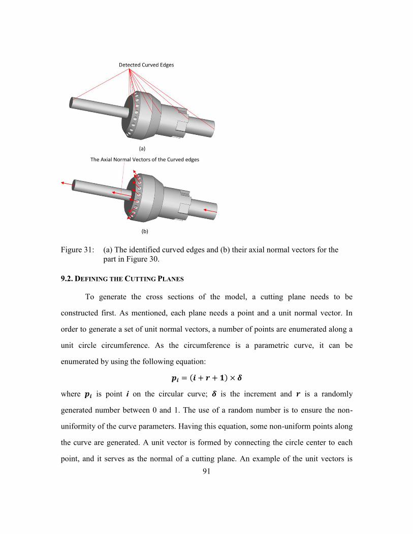
91
Figure 31: (a) The identified curved edges and (b) their axial normal vectors for the
part in Figure 30.
9.2. DEFINING THE CUTTING PLANES
To generate the cross sections of the model, a cutting plane needs to be
constructed first. As mentioned, each plane needs a point and a unit normal vector. In
order to generate a set of unit normal vectors, a number of points are enumerated along a
unit circle circumference. As the circumference is a parametric curve, it can be
enumerated by using the following equation:
where is point i on the circular curve; is the increment and is a randomly
generated number between 0 and 1. The use of a random number is to ensure the non-
uniformity of the curve parameters. Having this equation, some non-uniform points along
the curve are generated. A unit vector is formed by connecting the circle center to each
point, and it serves as the normal of a cutting plane. An example of the unit vectors is
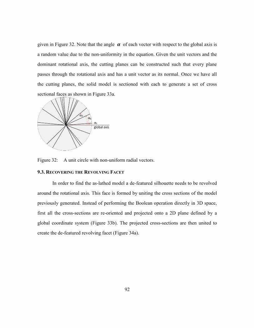
92
given in Figure 32. Note that the angle of each vector with respect to the global axis is
a random value due to the non-uniformity in the equation. Given the unit vectors and the
dominant rotational axis, the cutting planes can be constructed such that every plane
passes through the rotational axis and has a unit vector as its normal. Once we have all
the cutting planes, the solid model is sectioned with each to generate a set of cross
sectional faces as shown in Figure 33a.
Figure 32: A unit circle with non-uniform radial vectors.
9.3. RECOVERING THE REVOLVING FACET
In order to find the as-lathed model a de-featured silhouette needs to be revolved
around the rotational axis. This face is formed by uniting the cross sections of the model
previously generated. Instead of performing the Boolean operation directly in 3D space,
first all the cross-sections are re-oriented and projected onto a 2D plane defined by a
global coordinate system (Figure 33b). The projected cross-sections are then united to
create the de-featured revolving facet (Figure 34a).

93
Figure 33: (a) The sampled cross sections of the part in Figure 30; (b) the union of all
the cross sections.
Figure 34: (a) The revolving face and the rotational axis; (b) the as-lathed model.
9.4. EXTRACTING TURNABLE AND NON-TURNABLE FEATURES
Figure 34 shows how the as-lathed model is formed by sweeping the revolving
facet around the rotational axis. The non-turnable volume is obtained by subtracting the
as-lathed model from the original CAD model. To create non-turnable machining
features, this negative volume is fed into the volume decomposition algorithm in [5], and

94
the outputs are the isolated features for machining, which are shown in Figure 35b. For
these features, AMFA is used to generate the separate machining plans.
To extract the turnable features, first the as-lathed model (Figure 34b) is
subtracted from the raw work-piece (typically a bounding cylinder) to get the turnable
removal volume. The volume is then fed into a volume decomposition module similar to
[5] to generate isolated features for turning (Figure 35a). These features are then
translated into a seed graph representation. In the following chapters, a graph grammar
based approach is introduced to automate the reasoning on the graph in order to define
the turning operations for these features.
Figure 35: (a) The decomposed turnable features; (b) the non-turnable features.
9.5. EFFICIENCY AND EFFECTIVENESS
To ensure that the non-uniformly sampled cutting planes effectively capture all
the features from the original geometry, a series of tests have been conducted on complex
real parts that have several acentric features (Figure 36). Based on the results, a set of
heuristics have been set up in the reasoning to guide the selection of the number of non-
uniform samples that are needed based on the part complexity. As compared to the
uniform-sampling based approach in which the increment needs to be small enough to
detect the minimal circumferential feature, the non-uniform approach is able to set the
sample cuts adaptively such that the initial cuts with small increments are always initiated

95
at regions with dense features while the cuts with large increments are used to capture
uniformly distributed features as well as regions with no feature at all.
In addition, the rotational axis is identified automatically and without using any
Boolean operations. The revolving facet is recovered using a 2D union operation as
opposed to a 3D operation. In light of the computationally expensive Boolean operations
that are associated with the existing techniques, our novel simplifications guarantee the
efficiency and effectiveness of the algorithm.
Figure 36: A summary of the tests on more complex parts.

96
Chapter 10: Setup Design Based On Tolerance Analysis
In manufacturing process planning, tolerance analysis is of particular importance
in that a part created by any process plan must comply with all tolerances specified by the
designer in order to meet certain engineering constraints. Over the past several decades,
researchers have been exploring numerous tolerance analysis techniques, including
tolerance chain [96], kinematic analogies based approach [97], [98], Vectorial
representation [99], T-map and M-map [100], [101], Monte Carlo simulation based
approach [102], [103], statistical approach [104], [105], and more [106]–[109]. However,
in general those approaches either involve complicated geometric manipulations (e.g.
Minkowski sum) in both Euclidean space and specific pre-defined configuration space, or
require a large amount of computational resources (e.g. sampling) for reliable results.
Due to these limitations, the approaches have yet to be embedded into automated
manufacturability reasoning tools such that the results can be directly used as heuristics
to guide the generation of optimal manufacturing plans.
In this work, the tolerance analysis is envisioned from a prognostic perspective.
As the designer interprets the design intentions as the tolerance specifications, the
knowledge that is otherwise hidden in the tolerance specs is extracted and encapsulated
into the turning sequencing reasoning such that the tolerances themselves can be
effectively used to guide the generation of optimal plans in terms of satisfying the
tolerances. The tolerance analysis based setup design proposed in this work is based on a
tolerance graph approach proposed in [110], and it involves two phases of effort:
1. Selection of setups
A setup refers to the act of positioning and clamping a part with respect to one or
a set of manufacturing datums such that the turning operation can be conducted. For the

97
setup design, we need to consider two types of errors that are introduced during the
turning process. The first is the setup error, which includes the locating errors, the
clamping distortion, and the geometrical and dimensional inaccuracy of the fixture. The
second error is the machine motion error, which is generally caused by the deviation of
the tool under cutting forces. Additionally, each tolerance is designed with respect to one
or more specific design datums, which will be used to inspect the tolerance. However in
manufacturing, these design datums are not always available as manufacturing datums
due to numerous constraints (space limitation, tool-part collision, surface accessibility,
etc.). The inconsistency between the design datums and manufacturing datums leads to
the stack-up of the two types of errors, which make the tolerances difficult to satisfy.
The objective in setup selection is to minimize the total number of setups that are
required to turn a part in order to avoid potential error stack-ups. For that, we prefer to
turn as many faces as possible in a single setup. As long as the setup is not changed, the
setup error remains constant, and it does not lead to the stack-up with the machine motion
error. Therefore the turning precision is best guaranteed.
2. Selection of manufacturing datums for each setup
In this phase, we perform the selection of two datums (one cylindrical and one
planar) in order to fully secure the part in a lathe. The cylindrical face is used to define
the orientation, and the size of the feature is considered in the tolerance specifications so
that only large cylindrical faces are specified as design datums. The planar face is only
used to confine the axial translation, in which case the size factor is not important. It is
proposed that the faces with tighter tolerances should be preferred over faces with looser
tolerances when selecting manufacturing datums in order to achieve a better precision.
While this datum selection strategy may violate the intention of the standardized
tolerances in the sense that the design datum for a particular tolerance is not necessarily

98
considered as the manufacturing datum, it is shown in later chapters that this strategy can
effectively improve the overall satisfaction for all tolerances, especially in cases where
multiple tolerances are specified for a part and the inconsistency of manufacturing
datums and design datums is often inevitable during machining. Since features with
tighter tolerances are intended to have higher precision, they introduce less setup error
when used as manufacturing datums during machining processes as compared to other
faces. In addition, our strategy can effectively eliminate the influence of the error stack-
up on the tighter tolerances, which are generally more vulnerable to the errors.
99
Chapter 11: Graph Grammar Based Reasoning
To automate the aforementioned setup design strategy, a novel graph grammar
based approach is presented in this chapter. The grammar reasoning is implemented using
a graph grammar software (GraphSynth) that was previously developed by Campbell
[11]. As shown in the flowchart in Figure 37, three rules are manually designed to
encapsulate all the required reasoning. When an as-lathed model is fed into the module,
the reasoning performed by the rules as shown in Figure 37 is triggered automatically on
the platform of GraphSynth and the output is the recommended turning sequence.
The input of the reasoning is the 2D drawing or the 3D CAD model of an as-
lathed model with geometric dimensioning and tolerancing included. First, the geometric
reasoning automatically converts the as-lathed model to a tolerance graph (see the left
section of Figure 37), which serves as the seed of phase 1. In the first phase, rule 1 is
called recursively to convert the tolerance graph to a setup graph (refer to the center
section of Figure 37). During the reasoning, the minimal setups are identified from the
tolerance graph and are stored in the setup graph. Phase 2 takes the setup graph as an
input, and performs the reasoning prescribed by rule 3 (refer to the right section of Figure
37). The reasoning first identifies the manufacturing datums from the graph for each
setup with the goal of prioritizing faces with tighter tolerances. Then the selected datums
are attached to the setups that are sequenced in an order defined by the knowledge in the
rule. After phase 2, a complete turning sequence is generated. For both phases, rule 2 is
used to update the tolerance graph and setup graph if applicable in order to facilitate the
reasoning (see the center and right sections of Figure 37). In the first example that
follows, rule 2 is inactive, and its meaning is explained in the second example in chapter
12.

100
Figure 37: Grammar reasoning flowchart for turning process planning.
Consider the as-lathed model shown in Figure 34b as an example. A 2D
engineering drawing of the part is given in Figure 38 with the user-defined tolerances
carefully labeled. For example, face 4 has a coaxiality tolerance of 0.02mm with face 7,
and face 10 has a perpendicularity tolerance of 0.01mm with face 1.
Figure 38: The CAD drawing of the part shown in Figure 34b.
+X

101
First, the 3D model (with associated GD&T data) or the 2D drawing is converted
to a tolerance graph (Figure 39) for the grammar reasoning to use. In the tolerance graph,
the geometric elements are represented by nodes, arcs and hyper-arcs. Nodes are used to
represent faces. For example, the cylindrical face 7 is represented by the node with name
“n7” and a label “cylindrical”. The label is a string stored in the data structure of the
node and is used to indicate the face type. If two nodes have a tolerance relationship
assigned to them, an arc will connect them with the normalized tolerance labeled on it.
Figure 39: The tolerance graph generated from the 2D drawing in Figure 38.
As discussed in [111], the tolerance normalization stems from the fact that every
tolerance essentially defines a minimal zone within which a feature in question must
locate. Therefore, a generalized angle can be determined from the tolerance zone such
that the feature will always remain inside the minimal zone as long as the deviation of the
feature from its ideal position (i.e. the center of the minimal zone) is less than this angle.

102
Figure 40 shows the generalized angle for the parallelism tolerance. As the tolerance zone
for parallelism resembles a 2D region, the angle is relatively easy to identify. However,
for 3D tolerance zones (e.g. position tolerances), the derivation is more complicated and
we refer interested readers to [111]. Considering that all generalized angles are in radians,
the rules can assign relative tightness between two tolerances by simply comparing their
angles. In Figure 39, the generalized angle in radians for each arc (indicating each
tolerance relationship) is labeled in the parenthesis following the arc’s name. For
instance, the 0.02mm perpendicularity tolerance between face 4 and face 7 is normalized
to 0.0095 radians.
Figure 40: The generalized angle of the parallelism tolerance.
The figure shows the front view of a cuboid with its top face milled out
The normalization has been strictly defined for datum-dependent tolerances,
including orientation tolerances (parallelism, perpendicularity, angularity, etc.), location
tolerances (position tolerance, symmetry, concentricity, etc.) and profile tolerances for
primitive features (line, planar surface, cylinder, polygons, etc.). But for datum-
independent tolerances like form tolerances (flatness, cylindricity, etc.), the definition
needs to be modified to include the form variations. In the current work we assume
perfect form of feature. For the orientation and position tolerances in Figure 39, they are
directly comparable after converted to the generalized angle representations.
Figure 39 also includes several hyper-arcs, which are special graph elements for
the designer to use in GraphSynth and are represented as polygons encompassing the
Ideal part
Machined
part
α

103
connected nodes. While an arc can only connect two nodes, a hyper-arc can connect as
many nodes as needed. In the tolerance graph, three hyper-arcs (named as “ha0 (Sr)” –
name ha0 followed by the label Sr in the parentheses, “ha1 (Sl)” and “ha2 (Sb)”) are
used to categorize the face nodes into three groups: Sb, Sl and Sr. Group Sl contains all
faces that are better turned from the positive X (+X) direction. For example, since face 11
is in Sl – referring back to Figure 38 – (+X) direction is a better choice for turning this
face. Similarly, group Sr contains all faces that are better turned from the negative X (-X)
direction. Faces that are accessible from both (-X) and (+X) directions are grouped into
Sb. After the tolerance graph is generated, a set of rules are called to reason on the graph
in order to study the turning sequences against the tolerance specifications.
Phase 1: selection of setups
The first grammar rule as shown in Figure 41a is designed to perform the setup
selection. The rule is of the form ( ) where the left hand side (L) includes elements
and conditions to be recognized and satisfied in the host graph (tolerance graph) while the
right hand side (R) indicates the transformations of those elements that have been
recognized in the host graph.
Since our objective is to minimize the total number of setups, we are interested in
the faces in Sb group as they can be turned from either (+X) or (-X) direction and
therefore can be merged into either Sr or Sl group. The tightest tolerance associated with
a face dictates which group the face is moved into. The L of the rule begins the reasoning
by first detecting a set of arcs in the tolerance graph that have one end in the Sb group.
Within this set, the arc with the tightest tolerance (represented as arc a0 in the L of the
rule) is recognized. The arc in the tolerance graph (Figure 39) that meets the two
conditions is arc a1. Since a1 connects face nodes n7 and n9, and it is already known that
n9 can only be turned from the (+X) direction, we move n7 from group Sb into group Sl,

104
meaning n7 will be turned in the same setup as n9. The manipulation of n7 is realized
automatically through a virtual transformation from L to R of rule 1. In the R of the rule,
arc a0 (mapped to a1 in the tolerance graph) that was previously captured in the L is
deleted and face n0 (mapped to n7 in the tolerance graph) becomes encompassed by
hyperarc ha1 (representing Sl group) instead of ha0 (representing Sb group). Since in this
tolerance graph there is only one face in Sb group, the rule is called only once. After this
transition, Sb becomes empty and is deleted by the rule (as seen in the R of the rule, ha0
no longer exists). As a result, the tolerance graph evolves into a setup graph as shown in
Figure 42.
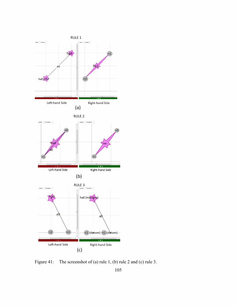
105
Figure 41: The screenshot of (a) rule 1, (b) rule 2 and (c) rule 3.

106
Figure 42: The screenshot of the setup graph.
In the setup graph, since the faces in Sl and Sr do not share common turning
directions, they have to be turned in two distinct setups. Therefore, we end up with two
minimal setups (Sl and Sr) after the setup selection. Next, we will select the
manufacturing datums for the two setups.
Phase 2: selection of manufacturing datums
The algorithm to select manufacturing datums is encoded into the third rule
shown in Figure 41c. Since each setup has multiple tolerances to satisfy, the
inconsistency of design and manufacturing datums is inevitable. For achieving a better
overall satisfaction for all tolerances, we prefer the faces with tighter tolerances as the
locating datums of each setup. Among all the remaining arcs in the setup graph (Figure
42: arcs a2, a3, a4, and a5), a4 is recognized as it represents the tightest tolerance.
Therefore face n1 and face n10 connected by a4 are intended to have the highest
precision. We can use face n1 as the locating datum of setup Sl, and face n10 as the
locating datum of setup Sr. Both faces will introduce less setup errors as compared to
other faces. Consider setup Sr first, the cylindrical datum n10 defines the orientation of
the part on the lathe. We still need a planar datum from the same group of n10 (Sl) in

107
order to constrain the translation of the part along X axis. While both face n9 and n11 are
available in Sl, n11 is selected as the second datum since it has a tighter tolerance
compared to n9. As a result, face n10 and n11 are chosen as the locating datums for setup
Sr.
Similarly, for setup Sl, the cylindrical face n4 is chosen with planar face n1 as the
locating datums. Note that n4 has a tighter tolerance compared to other cylindrical faces
in the same group. As represented in the third rule (Figure 41c), the two datum faces are
first recognized in the L as nodes n1 and n2. After the transformation from the L to the R,
the two nodes are assigned a new label “datum”, which indicates that the two datum
faces have been determined.
The last step of reasoning in phase 2 is to decide the setup sequence, or which
group (Sl or Sr) of faces to create first. This involves a concept of the Number of
Tolerances (NoT) associated with a face node, which is equivalent to the total number of
arcs incident on the node. The algorithm suggests that the group in which the face with
the highest NoT resides should be machined first. For this part, since face n1 has the
highest NoT (NoT = 2), Sr group should be turned fist. This is to guarantee more faces
are created in the early setups. The final setup sequence is shown in Figure 43, which is
effectively defined by the order in which the three grammar rules are called.

108
Figure 43: The suggested turning sequence for the part shown in Figure 34b.

109
Chapter 12: Detailed Example
As a more complex example, the part shown in Figure 44b is presented to further
explain our reasoning. Although there are interacting non-turnable features in the part, the
geometric reasoning is capable of recovering the as-lathed model (Figure 44a) for the
grammar reasoning to use. This conversion takes place within 0.135 seconds6 using C++
code and Parasolid kernel [112]. Then, the non-turnable volume (Figure 44c) is
decomposed into non-turnable features (Figure 44d) automatically within 0.19 seconds.
Due to space limitations, only the reasoning about the as-lathed model is described
below.
Figure 44: A complex part with interacting features.
The 2D drawing for the as-lathed model is shown in Figure 45 and the
corresponding tolerance graph is given in Figure 46. Note that, there are two arcs (a2 and
a4) located entirely inside Sl and Sr respectively. In our methodology, faces in the same
group are always turned in one setup for achieving the highest precision. Therefore, it is
assumed that the tolerances represented by these internal arcs are automatically satisfied
within their setup and there is no need to consider them in the later reasoning. The second
6 With no further specifications, all experiments in this part were implemented on a desktop computer with
AMD 3.2 GHz processor and 6 GB of memory.

110
rule in Figure 41b is specially designed to delete arcs of this kind before other rules start
the reasoning. If a tolerance graph does not have internal arcs (as in the first example),
then rule 2 will not be invoked.
Figure 45: The CAD drawing of the as-lathed model in Figure 44a.
Figure 46: The tolerance graph for the part shown in Figure 44a.
+X

111
Figure 47: The updated tolerance graph for the part shown in Figure 44a.
The internal arcs a2 and a4 are deleted.
After the update, the new tolerance graph is shown in Figure 47. Starting from the
new graph, similar reasoning is implemented to design the setups. First, rule 1 (Figure
41a) is called to evolve the tolerance graph into a setup graph, during which face n6 in Sb
is moved to Sr. This step is to minimize the number of setups such that the potential error
stack-ups can be avoided to the maximal extent. The resulted setup graph is shown in
Figure 48. Note that, after face n6 is moved to Sr group, arc a5 and a6 become internal
arcs and therefore are deleted by the second rule (Figure 41b). Next, rule 3 (Figure 41c) is
called to select the locating datums for the two remaining setups. The objective in this
phase is to prioritize the tightest tolerance a3 among the three remaining tolerances
(Figure 48: a0, a1, and a3). Therefore face n11 is preferred as the planar datum for Sl.
Meanwhile cylindrical face n6 that has the highest precision is chosen as the second
datum to fully secure the work-piece. For setup Sl, the pair of datums with highest
precision are face n3 and face n4. After the datum selection, the setup sequencing is also

112
performed during the call of rule 3. In this case, face n6 has the highest NoT (NoT = 2),
therefore the faces in Sr are turned first.
Figure 48: The setup graph for the part in Figure 44a.
The internal arcs a5 and a6 are deleted.
The complete grammar reasoning takes 0.18 seconds and the suggested turning
sequence is shown in Figure 49.
Figure 49: The suggested turning sequence for the part shown in Figure 44a.

113
Chapter 13: Plan Validation
After a turning sequence is generated, it is critical to verify if the plan achieves a
better performance in satisfying all the design tolerances. The author was working with
colleagues in Palo Alto Research Center to develop a real-time tolerance analysis module
for use in the automated manufacturing process planning tools [12]. The module takes in
a complete manufacturing plan as well as the part with all its tolerance specs. Then the
tolerance analysis technique performs a sampling based reasoning on the inputs. The
outputs from the reasoning are the acceptance rates for all design tolerances. An
acceptance rate is a stochastic estimation of the quality of a plan in terms of satisfying a
specific tolerance.
Two types of errors are discerned in simulating the manufacturing processes. The
first is the local manufacturing error that comes from the actual machining of a feature in
question. For example, the positioning inaccuracy of a machine and the spinning
deflection of a tool are common sources for this error. The second is the stack-up error,
which is due to the inconsistency between the manufacturing datums used to machine a
feature and the design datums used when inspecting the tolerance of the feature. When
machining the feature, design datums are not always available for use as manufacturing
datums due to numerous constraints (space limitation, tool-part collision, surface
accessibility, etc.). If the feature is machined with respect to other manufacturing datums,
variations from these datums will stack up with the variations of design datums during
the tolerance inspection, which makes the tolerance difficult to satisfy.
The tolerance analysis technique in [12] systematically analyzes the local
manufacturing error and the stack-up error. First, a set of points are sampled on a feature
to be analyzed. For each point, we then sample from error distributions that model the

114
local manufacturing error. By accumulating sampled errors onto the ideal location of
each point, we are able to get a stochastic estimation of the discretized feature after
machining. For a datum-independent tolerance, the estimated locations are evaluated
through membership tests against the Design Tolerance Zone (DTZ) that is explicitly
specified by the tolerance and the tolerance satisfaction can be assessed.
For the stack-up error, the idea is that every datum (design or manufacturing
datum) applies a homogeneous transformation onto the feature when it is used to locate
the feature. If the datum has a perfect form, this transformation is essentially an identity
transformation – meaning that the position and orientation of the feature are not changed
during alignment. Variation of a datum is caused by its local manufacturing error, and
may be bounded by a Manufacturing Tolerance Zone (MTZ) that is determined by the
manufacturing precision when creating the datum. Following a process plan, we can
extract a chain of datums that have been involved in the machining and inspection of the
feature in question. For each datum, a transformation is sampled in six Degrees of
Freedom (DOF) within its MTZ to describe the variation. Then the stack-up of the
variations in DTZs and MTZs can be implicitly represented by the composition and
intersection of all the relevant transformations in a sequence decided by the
manufacturing plan.
For a datum-dependent tolerance, the stack-up error represented by
transformations is accumulated with the local manufacturing error. The results are
compared with the explicitly specified DTZ in order to compute the tolerance satisfaction
rate.
For the purpose of evaluating the quality of our plans, we conduct a comparative
study using the tolerance analysis module. We take the part in Figure 34b as a case to
study. The plan generated by our reasoning in Figure 43 is used as the first sample. To

115
make our experiment general, we propose a traditional turning plan as shown in Figure
50 for comparison. As compared to the suggested plan, this plan creates face 7 in setup 1
and uses different locating datums in setup 2. It is an obvious plan that one may bring up
without considering any tolerances.
Figure 50: A traditional turning sequence for the part shown in Figure 34b.
The tolerance analysis module is used to analyze both plans. To make the
comparative results more prominent, we set the maximum variations of all error sources
(machine error, tool error, locating error, etc.) to be 0.02 mm with a 95% confidence
interval, which are of the same scale as the tolerance specs. The results are summarized
in Table 13.
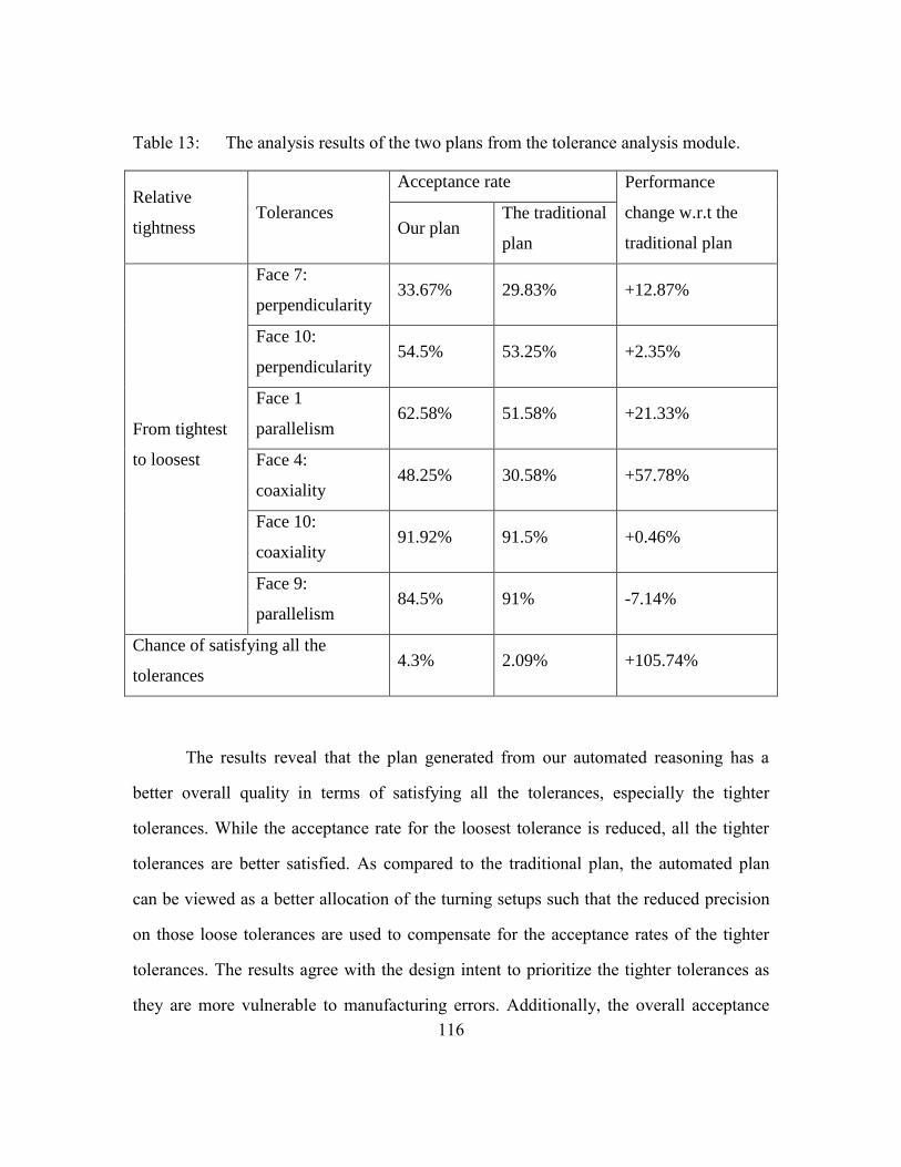
116
Table 13: The analysis results of the two plans from the tolerance analysis module.
Relative
tightness Tolerances
Acceptance rate Performance
change w.r.t the
traditional plan Our plan
The traditional
plan
From tightest
to loosest
Face 7:
perpendicularity 33.67% 29.83% +12.87%
Face 10:
perpendicularity 54.5% 53.25% +2.35%
Face 1
parallelism 62.58% 51.58% +21.33%
Face 4:
coaxiality 48.25% 30.58% +57.78%
Face 10:
coaxiality 91.92% 91.5% +0.46%
Face 9:
parallelism 84.5% 91% -7.14%
Chance of satisfying all the
tolerances 4.3% 2.09% +105.74%
The results reveal that the plan generated from our automated reasoning has a
better overall quality in terms of satisfying all the tolerances, especially the tighter
tolerances. While the acceptance rate for the loosest tolerance is reduced, all the tighter
tolerances are better satisfied. As compared to the traditional plan, the automated plan
can be viewed as a better allocation of the turning setups such that the reduced precision
on those loose tolerances are used to compensate for the acceptance rates of the tighter
tolerances. The results agree with the design intent to prioritize the tighter tolerances as
they are more vulnerable to manufacturing errors. Additionally, the overall acceptance

117
rate, which is interpreted as the chance of satisfying all the tolerances, is doubled in our
new plan (4.3% compared to 2.1%). Two insights can be drawn from the final
percentages: 1) By leveraging the performance on tighter tolerances, our algorithm is able
to improve the overall plan quality significantly; 2) Despite the doubled acceptance rate,
the manufacturing is poorly able to meet all these tolerance requirements. It signifies that
the designer ought to rethink of the tight tolerance specifications in light of the existing
manufacturing capabilities.

118
Chapter 14: Part II Summary
A novel approach for automating the turning process planning for mill-turn parts
is presented in this part. The algorithm starts by identifying the dominant rotational axis
from a mill-turn part and performing several non-uniform longitudinal cross-sectional
cuts to quickly generate the as-lathed model. Then several simple Boolean operations are
implemented to successfully generate both the turnable and non-turnable features. For the
non-turnable features, AMFA is employed to automatically generate the optimal process
plans in terms of manufacturing time, cost and fixture quality.
For the turnable features, the turning sequences are designed based on the analysis
of the knowledge that is conveyed in the tolerances specified by the designer. Given a set
of turnable features with multiple tolerances attached, the inconsistency between design
datums and manufacturing datums is often inevitable. It is therefore hard to decide which
faces to use as manufacturing datums when turning the features in order to achieve the
best tolerance satisfaction. The tolerance based reasoning streamlines the turning setup
design with a two-phase strategy: 1) selection of setups and 2) selection of manufacturing
datums for each setup. In phase 1, we design the setups in a way that every setup creates
as many features as possible. As a result, the number of setups required is minimized and
the potential error stack-up is avoided to the maximum extent. In phase 2, two faces (a
cylindrical face and a planar face) are selected to fully secure the work-piece for each
setup. During the selection, we prioritize faces with tighter tolerances as manufacturing
datums because they are intended to have higher precisions and therefore lead to less
setup errors as compared to other faces.
A rule-based grammar reasoning scheme has been developed to automatically
implement such reasoning and generate turning sequences that satisfy the tolerance

119
requirements. The reasoning differs from the existing turning process planning
techniques in that it extracts knowledge directly from the design tolerances and uses the
knowledge to dictate the generation of optimal turning sequences. We have demonstrated
that the information conveyed in the tolerances is critical to ensure that the suggested
process plans are able to significantly improve the turning precision.
As compared to the existing tolerance analysis techniques, our approach is
prognostic rather than diagnostic in the sense that the tolerances are used as heuristics to
guide the generation of optimal plans instead of being used to validate an existing plan. In
addition, since it reasons directly on the tolerances, much less computation is required as
the large-scale sampling of the manufacturing processes that is often performed in
traditional tolerance analysis is no longer necessary. As a result, the efficiency of our
reasoning is preserved.

120
Chapter 15: Conclusion
This chapter summarizes the work in the dissertation and highlights the
contributions and novelty. The potential directions of further study are also discussed.
The chapter ends with closing remarks.
15.1. SUMMARY
A complete and systematic approach to reasoning about the manufacturability of
any solid model is demonstrated in this dissertation. It consists of two modules: the
Automated Manufacturability Feedback Analysis (AMFA) that is developed to propose
optimal process plans in time, cost and fixture quality for non-turning operations, and the
turning process planning module that generates feasible turning sequences for achieving
the best tolerance satisfaction. For complex mill-turn parts, the approach is able to
automatically separate the turnable features for turning process planning and the non-
turnable features for AMFA. The process plans for non-turnable features are detailed
with the amount of material to remove, the suggested tools and machines, the precise feed
directions, the optimal fixture mechanisms to secure the work-piece and the estimated
time and cost for machining. Numerous real parts provided by our industrial and research
partners are used to validate the optimality and practicality the suggested plans. The real
implementations of two suggested plans in the machine shop are also provided. The
results show the consistency between the suggested plans and tooling parameters from
AMFA and the actual choices on the shop floor.
For the turnable features, the suggested turning sequences articulate the required
setups and the features to be created at each setup in order to best satisfy the prescribed
tolerances. Each setup includes a cylindrical face that is used to define the orientation of
the work-piece and a planar face that is used to constrain the axial translation of the

121
work-piece in the lathe. The preferred sequence and feed directions for turning the
features in each setup are also provided. Two mill-turn parts are used to demonstrate the
validity of our algorithm. One of the suggested turning sequences is compared with a
manually proposed plan from expert machinist using a separate tolerance analysis module
in which the tolerance satisfactions for both plans are assessed. The results show the
effectiveness and optimality of our plans in satisfying all the prescribed tolerances.
15.2. CONTRIBUTIONS AND NOVELTY
Three major engineering problems are addressed in this dissertation: the
computer-aided manufacturing process planning (CAPP), the computer-aided fixture
design (CAFD), and the automated turning process planning.
1. For CAPP, we demonstrate a graph grammar based approach to
automatically define detailed manufacturing process plans for complex solid
models. The graph lexicon preserves all necessary geometric and topological
information of the solid model that is relevant to the manufacturability analysis
and enables an accurate reasoning of the manufacturing process planning for
complex geometries. The approach is very efficient as it is structured in a way
that the computationally intensive geometric reasoning is separated from the
grammar based manufacturability analysis, which has not been seen in the
existing research.
2. The CAFD solution proposed here is seamlessly integrated into AMFA and it
allows us to identify the dependency between the fixture design and the
manufacturing process planning, which has not been well explored in
existing literatures. Through a set of case studies, the necessity of thoroughly
122
assessing the manufacturing dependency is shown for defining optimal process
plans and fixture designs.
3. The CAFD algorithm uses the manufacturing knowledge and experience
instead of the conventional multi-disciplinary design optimization techniques
to define the optimality of a fixture design. The algorithm is particularly
efficient as it avoids the complicated and inefficient computations in the early
stage of fixture design. In addition, the practicality of the suggested fixtures is
guaranteed by the empirical knowledge used to guide the generation of optimal
solutions.
4. The automated turning process planning algorithm in the dissertation shifts
the view of the tolerance analysis from a diagnostic perspective to a
prognostic aspect. We extract the knowledge that is otherwise hidden in the
tolerances and use it directly to decide the optimal sequences of turning
operations. The approach is effective as it takes tolerances into consideration at
every stage of the reasoning, which closely matches the design intentions.
Compared to the existing tolerance analysis techniques that are typically used to
validate a given process plan, our approach is able to generate plans that are
proven to be optimal in satisfying all the tolerances. This way, the tolerance
analysis after machining becomes easier and the manufacturing efficiency is
improved.
5. In this work we also develop a hierarchical sorting based best first search
technique and demonstrate its efficiency and effectiveness in solving multi-
objective optimization problems in manufacturing domains (e.g. machining
process planning, and assembly/disassembly process planning). We have
validated the linear-time convergence of the search technique to optimal

123
solutions. The rationale behind the new search is that the domain-specific
knowledge can not only be used to define evaluation metrics in the optimization
but also used to tailor the sorting strategy in order to yield practical results.
15.3. FUTURE WORK
15.3.1. Tool path generation
The current process planning algorithms specifies the optimal sequences of
operations that are required to create the final shape of a CAD model. For the plans to be
readily implementable on the shop floor, especially in a CNC machining environment,
the precise tool path for each operation is required. A complete tool path for a given
operation includes air cut and non-air cut. During the non-air cut, the tool is engaged with
the removal material and the tool motion is directly used to cut off required material from
the work-piece. Given a region of material to remove, the tool path for the non-air cut is
closely related to the geometry of the removal material and the tooling parameters. Two
types of non-air cut tool paths that are widely used in the foundry are the contour tool
path (Figure 51) and the zigzag tool path (Figure 52). Further efforts are needed to
encode the tool paths in the context of prescribed tooling environment.

124
Figure 51: 2D contour tool path7.
Figure 52: The zig-zag tool path projected onto a milling surface8.
The air-cut is also critical as it provides the tool proper lead-in and lead-out
directions before and after an operation, which is critical to keep the tool from sudden
changes of cutting forces. It also defines the motion of the tool between regions of
removal material that are not inter-connected. The motion needs to be carefully planned
in order to save the air-cut time and to avoid the collision of the tool with environmental
obstacles (e.g. fixtures, jigs, machine table and spindle, etc.). Given the sizes of the tool
7 Excerpted from http://www.hsmworks.com/docs/cncbook/en/#Ch07_2DContour. 8 Excerpted from
http://www.ezcam.com/web/products/help/ezmill/machining_mill_2d/projection_&_zig_zag_graphic.htm.

125
and the obstacles, the automated tool path planning is often a very complicated
optimization problem that involves Boolean operations of rigid bodies in 3D space. In
addition, for the continuous tool movements between any two consecutive operations,
each individual tool path planning problem needs to be considered collectively. Extensive
research is required to address all the concerns before a complete and optimal tool path
for a given process plan can be generated.
15.3.2. Fixture unit design
In this dissertation we limit the fixture mechanisms to the downward clamping
and the side clamping, and only consider the fixture faces used for each mechanism. In
high-production foundry where the modular fixtures are often desired, the actual
locations on each fixture face that are used to engage with the modular fixtures (e.g. pin-
array fixture) need to be computed. Since in our reasoning we already identify feasible
regions within every fixture face for clamping and locating, the fixture unit design
problem is greatly simplified as there is no need to blindly search every face of the
geometry in order to find the best ones. However, the selection of contacting points on
our suggested face regions still requires specific algorithm (for example, a typical
technology used is the Ray-tracing algorithm) to be employed, in which the force and
stress distribution, the spatial interference, and the clamping and locating strategies need
to be considered collectively.
15.3.3. Tolerance analysis in non-turning process planning
Currently tolerance analysis is only used in the automated turning process
planning in the dissertation. In non-turning process planning, the tolerances are of equal
importance to ensure that the part created meets all engineering constraints. The idea of
analyzing the prescribed tolerances in order to guide the generation of optimal process

126
plans can be extended to AMFA as well. The knowledge conveyed by the tolerances can
be used as another heuristic in the hierarchical sorting based best first search such that the
suggested plan is also assessed in terms of tolerance satisfaction. The only problem with
this strategy is the need of a new hierarchy for the extended set of metrics. It is expected
that a second study of the problem will avail the setup of the hierarchy in order to yield
practical and optimal solutions.
15.3.4. System integration
Above the aforementioned directions, the ultimate task is to integrate the separate
reasoning for turning and non-turning operations into a synthesized approach. Currently,
the differentiation of the turning process and the non-turning process may prevent some
optimal plans from being generated. For instance, in a machining center it is possible for
a milling tool to machine certain turnable features as well. In the integrated system the
turning and milling processes will be alternative options for the turnable features (for
non-turnable features, turning operations will never be invoked simply because it is
highly unlikely that these features can be machined in turning process). This way, the
automated reasoning can be performed on complex mill-turn parts that require solely
milling processes.
With the system integration, we will be able to develop a complete graph
grammar based system that is able to reason about all subtractive manufacturing
processes and geometries of different complexity and generate optimal manufacturing
plans in terms of any user-specified objectives.

127
15.4. CLOSING REMARKS
The computational approach presented here streamlines the design and digital
manufacturing by synthesizing the multi-disciplinary knowledge across geometry,
manufacturing, fixture, tolerance analysis and generative search while providing
automated feedback for optimal design and manufacturing. The resulting tool can help
industries in improving manufacturing efficiency, precision, and cost and catalyzing
product designs with better manufacturability.

128
Bibliography
[1] T. Dong, L. Zhang, R. Tong, and J. Dong, “A hierarchical approach to disassembly
sequence planning for mechanical product,” Int. J. Adv. Manuf. Technol., vol. 30,
no. 5–6, pp. 507–520, Dec. 2005.
[2] Q. Guan, J. H. Liu, and Y. F. Zhong, “A concurrent hierarchical evolution
approach to assembly process planning,” Int. J. Prod. Res., vol. 40, no. 14, pp.
3357–3374, Jan. 2002.
[3] W. Fu, A. A. Eftekharian, and M. I. Campbell, “AUTOMATED
MANUFACTURING PLANNING APPROACH BASED ON VOLUME
DECOMPOSITION AND GRAPH-GRAMMARS,” J. Comput. Inf. Sci. Eng., vol.
13, no. 2, 2013.
[4] A. Nagpal, “A hierarchical approach to process planning,” University of Windsor,
1989.
[5] A. Eftekharian and M. I. Campbell, “Convex Decomposition of 3D Solid Models
for Automated Manufacturing Process Planning Applications,” in ASME 2012
International Design Engineering Technical Conferences & Computers and
Information in Engineering Conference (IDETC/CIE), 2012.
[6] A. A. Eftekharian, W. Fu, C. Manion, and M. I. Campbell, “Automatic Reasoning
for Defining Lathe Operations for Mill-Turn Parts,” in Proceedings of the ASME
2013 International Design Engineering Technical Conference & Computers and
Information in Engineering Conference IDETC/CIE 2013, 2013, no. 512, pp. 1–11.
[7] W. Fu, A. Eftekharian, P. Radhakrishnan, M. Campbell, and C. Fritz, “A GRAPH
GRAMMAR BASED APPROACH TO AUTOMATED MANUFACTURING
PLANNING,” in ASME 2012 International Design Engineering Technical
Conferences & Computers and Information in Engineering Conference
(IDETC/CIE), 2012, no. 512.
[8] W. Fu and M. I. Campbell, “Concurrent Fixture Design for Automated
Manufacturing Process Planning,” Int. J. Adv. Manuf. Technol., pp. 1–22, 2014.
[9] W. Fu, A. A. Eftekharian, M. I. Campbell, and T. Kurtoglu, “Automatic Reasoning
for Defining Lathe Operations For Mill-Turn Parts: A Tolerance Based Approach,”
J. Mech. Des., 2013.
[10] Delcam Advanced Manufacturing Solutions, “FeatureCAM.” [Online]. Available:
http://www.featurecam.com/.

129
[11] M. I. Campbell, “GraphSynth2: software for generative grammars and creative
search,” 2012. [Online]. Available: https://bitbucket.org/MattCampbell/graphsynth.
[12] W. Fu, S. Nelaturi, A. Rangarajan, and T. Kurtoglu, “Tolerance Analysis for
Validating Manufacturing Process Plans,” in Proceedings of the ASME 2014
International Design Engineering Technical Conferences & Computers and
Information in Engineering Conference (IDETC/CIE), 2014.
[13] E. L. Russell, Automated Manufacturing Planning. New York: American
Management Association, 1967.
[14] H. R. Berenji and B. Khoshnevis, “Use of artificial intelligence in automated
process planning,” Comput. Mech. Eng., vol. 5, no. 2, pp. 47–55, 1986.
[15] G. Chryssolouris, S. Chan, and N. P. Suh, “An Integrated Approach to Process
Planning and Scheduling,” CIRP Ann. - Manuf. Technol., vol. 34, no. 1, pp. 413–
417, Jan. 1985.
[16] P. Taylor, H. B. E. N. Wang, R. A. Wysk, and L. D. B. Hall, “A knowledge-based
approach for automated process planning,” Int. J. Prod. Res., vol. 26, no. 6, 1988.
[17] H. B. Marri, A. Gunasekaran, and R. J. Grieve, “Computer-Aided Process
Planning: A State of Art,” Int. J. Adv. Manuf. Technol., vol. 14, pp. 261–268, 1998.
[18] R. Sharma and J. X. Gao, “Implementation of step 224 in an automated
manufacturing planning system,” Proc. Inst. Mech. Eng. Part B Eng. Manuf., vol.
216, no. 9, pp. 1277–1289, 2002.
[19] R. D. Allen, J. A. Harding, and S. T. Newman, “The application of STEP-NC
using agent-based process planning,” Int. J. Prod. Res., vol. 43, pp. 655–670, 2005.
[20] H. Ehrig, G. Engels, H. J. Kreowski, and G. Rozenberg, Handbook of Graph
Grammars and Computing by Graph Transformations. NJ: World Science
Publication Co., 1999.
[21] F. L. Krause, Product Modeling: An Approach for Integrated Information
Processing. Springer Berlin Heidelberg, 1993, pp. 160–175.
[22] A. P. Rockwood, “Geometric primitives,” ACM Comput. Surv., vol. 28, no. 1, pp.
149–151, Mar. 1996.
[23] F. Krause, F. Kimura, T. Kjellberg, S. C. Lu, I. Suh, V. A. Tipnis, and M. I. Weck,
“Product Modelling,” vol. 42, no. 2, pp. 695–706, 1993.

130
[24] J. Han, M. Pratt, and W. C. Regli, “Manufacturing feature recognition from solid
models: a status report,” IEEE Trans. Robot. Autom., vol. 16, no. 6, pp. 782–796,
2000.
[25] J. J. Shah, “Assessment of features technology,” Comput. Des., vol. 23, no. 5, pp.
331–343, Jun. 1991.
[26] J. J. Shah, D. Anderson, Y. S. Kim, and S. Joshi, “A Discourse on Geometric
Feature Recognition From CAD Models,” J. Comput. Inf. Sci. Eng., vol. 1, no. 1, p.
41, 2001.
[27] S. Subrahmanyam and M. Wozny, “An overview of automatic feature recognition
techniques for computer-aided process planning,” Comput. Ind., vol. 26, no. 1, pp.
1–21, Apr. 1995.
[28] B. Babic, N. Nesic, and Z. Miljkovic, “A review of automated feature recognition
with rule-based pattern recognition,” Comput. Ind., vol. 59, no. 4, pp. 321–337,
Apr. 2008.
[29] M. Marefat and R. L. Kashyap, “Geometric reasoning for recognition of three-
dimensional object features,” IEEE Trans. Pattern Anal. Mach. Intell., vol. 12, no.
10, pp. 949–965, 1990.
[30] T. Laakko and M. Miintylii, “Feature modeling by incremental feature recognition,”
Comput. Des., vol. 25, no. 8, pp. 479–492, 1993.
[31] S. Joshi and T. C. Chang, “Graph-based heuristics for recognition of machined
features from a 3D solid model,” Comput. Des., vol. 20, no. 2, pp. 58–66, Mar.
1988.
[32] S. N. Trika, S. Member, and R. L. Kashyap, “Geometric Reasoning for Extraction
of Manufacturing Features in Iso-Oriented Polyhedrons,” IEEE Trans. Pattern
Anal. Mach. Intell., vol. 16, no. 11, pp. 1087–1100, 1994.
[33] B. V. S. Kumar and C. S. P. Rao, “Automatic Extraction of Three Dimensional
Prismatic Machining Features from CAD Model,” Int. J. Comput. Sci. Commun.
Networks, vol. 1, no. 3, pp. 285–296.
[34] M. Sadaiah, D. R. Yadav, P. V Mohanram, and P. Radhakrishnan, “A Generative
Computer-Aided Process Planning System for,” Int. J. Adv. Manuf. Technol., vol.
20, pp. 709–719, 2002.
131
[35] H. K. D. Bouzakis and G. Andreadis, “A feature-based algorithm for computer
aided process planning for prismatic parts,” Int. J. Prod. Eng. Comput., vol. 3, no.
3, pp. 17–22, 2000.
[36] M. Henderson and D. Anderson, “Computer Recognition and Extraction of Form
Features : A CAD / CAM Link,” Comput. Ind., vol. 5, pp. 329–339, 1984.
[37] V. B. Sunil and S. S. Pande, “Automatic recognition of features from freeform
surface CAD models,” Comput. Des., vol. 40, no. 4, pp. 502–517, Apr. 2008.
[38] Y. S. Kim, E. Wang, and H. M. H. M. Rho, “Geometry-based machining
precedence reasoning for feature-based process planning,” Int. J. Prod. Res., vol.
39, no. 10, pp. 2077–2103, Jan. 2001.
[39] V. SHAPIRO, “Well-formed set representations of solids,” Int. J. Comput. Geom.
Appl., vol. 9, pp. 125–150, 1999.
[40] S. B. Tor and A. E. Middleditch, “Convex Decomposition of Simple Polygons,”
ACM Trans. Graph., vol. 3, no. 4, pp. 244–265, Oct. 1984.
[41] D. Dobkin, L. Guibas, and J. Hershberger, “An Efficient Algorithm for Finding the
CSG Representation of a Simple Polygon,” ACM Trans. Graph., vol. 22, no. 4, pp.
31–40, 1988.
[42] T. Woo, “Feature Extraction by Volume Decomposition,” in CAD/CAM
Technology in Mechanical Engineering, 1982.
[43] Y. S. Kim and D. J. Wilde, “A Convex Decomposition Using Convex Hulls and
Local Cause of Its Non-Convergence,” J. Mech. Des., vol. 114, no. September
1992, 1992.
[44] Y. S. Kim, “Recognition of form features using convex decomposition,” Comput.
Des., vol. 24, no. 9, pp. 461–476, Sep. 1992.
[45] C. Ertelt and K. Shea, “An application of shape grammars to planning for CNC
machining,” in the ASME 2009 International Design Engineering Technical
Conferences & Computers and Information in Engineering Conference
IDETC/CIE, 2009.
[46] H. Wang, Y. (Kevin) Rong, H. Li, and P. Shaun, “Computer aided fixture design:
Recent research and trends,” Comput. Des., vol. 42, no. 12, pp. 1085–1094, Dec.
2010.

132
[47] D. Bourne, J. Corney, and S. K. Gupta, “Recent Advances and Future Challenges
in Automated Manufacturing Planning,” J. Comput. Inf. Sci. Eng., vol. 11, no. 2,
pp. 021006–01, 2011.
[48] Y. Sermsuti-anuwat, “Milling fixture design: a tolerance analysis approach,” Int. J.
Mech. Eng. Educ., vol. 37, no. 2, pp. 111–118, 2009.
[49] Y. Kang, Y. Rong, and J. C. Yang, “Computer-Aided Fixture Design Verification .
Part 2 . Tolerance Analysis,” Int. J. Adv. Manuf. Technol., vol. 21, pp. 836–841,
2003.
[50] J. S. Pang and J. C. Trinkle, “Stability characterizations of fixtured rigid bodies
with Coulomb friction,” Proc. 2000 ICRA. Millenn. Conf. IEEE Int. Conf. Robot.
Autom. Symp. Proc. (Cat. No.00CH37065), vol. 1, pp. 361–368.
[51] Y. Kang, Y. Rong, and J. C. Yang, “Computer-Aided Fixture Design Verification.
Part 3. Stability Analysis,” Int. J. Adv. Manuf. Technol., vol. 21, pp. 842–849,
2003.
[52] L. Fan, B. N. Jagdish, A. S. Kumar, S. Anbuselvan, and S. Bok, “Collaborative
Fixture Design and Analysis Using Service Oriented Architecture,” IEEE Trans.
Autom. Sci. Eng., vol. 7, no. 3, pp. 617–629, 2010.
[53] B. Dizioglu and K. Lakshiminarayana, “Mechanics of Form Closure,” Acta Mech.,
vol. 118, pp. 107–118, 1984.
[54] X. Markenscoff and C. H. Papadimitriou, “The Geometry of Grasping,” Int. J. Rob.
Res., vol. 9, no. 1, pp. 61–74, Feb. 1990.
[55] A. F. Van der Stappen, C. Wentink, and M. H. Overmars, “Computing form-
closure configurations,” Proc. 1999 IEEE Int. Conf. Robot. Autom. (Cat.
No.99CH36288C), vol. 3, no. May, pp. 1837–1842, 1999.
[56] R. a. Marin and P. M. Ferreira, “Optimal Placement of Fixture Clamps:
Maintaining Form Closure and Independent Regions of Form Closure,” J. Manuf.
Sci. Eng., vol. 124, no. 3, pp. 676–685, 2002.
[57] Y. Zheng and C.-M. Chew, “Efficient Procedures for Form-Closure Grasp
Planning and Fixture Layout Design,” J. Manuf. Sci. Eng., vol. 131, no. 4, pp.
041010–1, 2009.

133
[58] C. Munro and D. Walczyk, “Reconfigurable Pin-Type Tooling: A Survey of Prior
Art and Reduction to Practice,” J. Manuf. Sci. Eng., vol. 129, no. 3, pp. 551–565,
2007.
[59] X. Xiaowen, X. Wei, and Z. Beirong, “Modular Reconfigurable Fixture Design
Based Intelligent Algorithm,” 2009 Int. Conf. Inf. Technol. Comput. Sci., pp. 156–
159, Jul. 2009.
[60] G. Wilson and J. P. Weaver, “Light fixture using modular accessories,” 2013.
[61] S. Zirmi, H. Paris, and I. Belaidi, “Analysis of modular fixtures design,”
Mécanique Ind., vol. 8, pp. 1–6, 2007.
[62] S. H. Sun and J. L. Chen, “A Fixture Design System using Case-based Reasoning,”
Eng. Appl. Artif. Intell., vol. 9, no. 5, pp. 533–540, 1996.
[63] J. Chang, “Methodology for automatic fixture design in a computer-integrated
environment,” Purdue University, 1989.
[64] J. Cecil, “Computer-Aided Fixture Design - A Review and Future Trends,” Int. J.
Adv. Manuf. Technol., vol. 18, no. 11, pp. 790–793, Nov. 2001.
[65] M. H. Yadav and S. S. Mohite, “Computer integrated fixture design system,” Proc.
Int. Conf. Work. Emerg. Trends Technol. - ICWET ’11, no. Icwet, p. 775, 2011.
[66] Y. Kang, Y. Rong, and J. C. Yang, “Computer-Aided Fixture Design Verification.
Part 1. The Framework and Modelling,” Int. J. Adv. Manuf. Technol., vol. 21, no.
10–11, pp. 827–835, Jul. 2003.
[67] Y.-J. Tseng and S. B. Joshi, “Recognition of interacting rotational and prismatic
machining features from 3-D mill-turn parts,” Int. J. Prod. Res., vol. 36, no. 11, pp.
3147–3165, 1998.
[68] D. L. Waco and Y. S. Kim, “Machining feature reasoning using convex
decomposition,” Adv. Eng. Softw., vol. 20, pp. 107–119, 1994.
[69] P. B. Berra and M. M. Barash, “Automatic process planning and optimization for a
turning operation,” Int. J. Prod. Res., vol. 7, no. 2, pp. 93–103, 1968.
[70] S. K. Lai-Yuen and Y.-S. Lee, “Turn-Mill Tool Path Planning and Manufacturing
Cost Analysis for Complex Parts Machining,” in Industrial Engineering Research
(IERC) Conference, 2002.

134
[71] X. Zhang, R. Liu, a. Nassehi, and S. T. Newman, “A STEP-compliant process
planning system for CNC turning operations,” Robot. Comput. Integr. Manuf., vol.
27, no. 2, pp. 349–356, Apr. 2011.
[72] S. Huang, D. Liu, and B. Wang, “Research on Lathe Automatic Design System,”
in 2009 International Conference on Management and Service Science, 2009.
[73] D. E. Culler, “The Turning Assistant : Automated planning for numerical control
lathe operations.” ProQuest Dissertation and Theses (PQDT), 1994.
[74] S. Liu, “FEATURE EXTRACTION AND CLASSIFICATION FOR
ROTATIONAL PARTS TAKING 3D DATA FILES AS INPUT,” J. Chinese Inst.
Ind. Eng., vol. 21, no. 5, pp. 432–443, 2004.
[75] S. Suliman and K. Awan, “Automatic Recognition of Turning Features Using 2-D
Drawing Files.,” JSME Int. J. Ser. C, vol. 44, no. 2, pp. 527–533, 2001.
[76] S. Li and J. J. Shah, “Recognition of User-Defined Turning Features for Mill/Turn
Parts,” J. Comput. Inf. Sci. Eng., vol. 7, no. 3, pp. 225–235, 2007.
[77] R. Dechter and R. Mateescu, “AND/OR search spaces for graphical models,” Artif.
Intell., vol. 171, no. 2–3, pp. 73–106, Feb. 2007.
[78] R. A. Walsh and D. R. Cormier, Machining and metalworking handbook, 3rd ed.
McGraw-Hill Companies, Inc., 2006.
[79] G. Boothroyd and W. A. Knight, Fundamentals of machining and machine tools,
3rd ed. Boca Raton, FL : CRC/Taylor & Francis, 2006.
[80] J. P. Davim, Ed., Machining : fundamentals and recent advances. London :
Springer, 2008.
[81] B. Van Blarigan, M. I. Campbell, A. Eftekharian, and T. Kurtoglu, “Automated
Estimation of Time and Cost For Determining Optimal Machining Plans,” in
ASME 2012 International Design Engineering Technical Conferences &
Computers and Information in Engineering Conference (IDETC/CIE), 2012.
[82] P. H. Joshi, Jigs and Fixtures Design Manual, 2nd ed. McGraw-Hill Companies,
Inc., 2003.
[83] Y. (Kevin) Rong and Y. (Stephens) Zhu, Computer-Aided Fixture Design, 1st ed.
New York: Marcel Dekker, Inc., 1999.

135
[84] Y. (Kevin) Rong, S. H. Huang, and Z. Hou, Advanced Computer-Aided Fixture
Design, 1st ed. Elsevier Academic Press, 2005.
[85] S. J. Russell, Artificial Intelligence: Modern Approach. pp. 73–110.
[86] R. T. Marler and J. S. Arora, “Survey of multi-objective optimization methods for
engineering,” Struct. Multidiscip. Optim., vol. 26, no. 6, pp. 369–395, Apr. 2004.
[87] L. Zadeh, “Optimality and non-scalar-valued performance criteria,” IEEE Trans.
Automat. Contr., vol. 8, no. 1, pp. 59–60, Jan. 1963.
[88] G. Anandalingam and T. L. Friesz, “Hierarchical Optimization: An Introduction,”
Ann. Oper. Res., vol. 34, pp. 1–11, 1992.
[89] T. Basar and H. Selbuz, “Closed-Loop Stackelberg Strategies with Applications in
the Optimal Control of Multilevel Systems,” IEEE Trans. Automat. Contr., vol.
AC-24, no. 2, pp. 166–178, 1979.
[90] M. Seder, P. Mostarac, and I. Petrovic, “Hierarchical path planning of mobile
robots in complex indoor environments,” Trans. Inst. Meas. Control, vol. 33, no.
3–4, pp. 332–358, Feb. 2010.
[91] R. Rajagopalan, K. G. Mehrotra, C. K. Mohan, and P. K. Varshney, “Hierarchical
Path Computation Approach for Large Graphs,” IEEE Trans. Aerosp. Electron.
Syst., vol. 44, no. 2, 2008.
[92] Y.-J. Lai, “Hierarchical optimization : A satisfactory solution,” Fuzzy Sets Syst.,
vol. 77, pp. 321–335, 1996.
[93] A. Autere, “Estimating search depths in hierarchical path planning,” in
Proceedings 1999 IEEE/RSJ International Conference on Intelligent Robots and
Systems, 1999, vol. 3, pp. 1304–1309.
[94] W. Jia and Z. Sun, “On Computational Complexity of Hierarchical Optimization,”
Int. J. Found. Comput. Sci., vol. 13, no. 5, pp. 667–670, 2002.
[95] W. Fu and M. I. Campbell, “Multi-objective Hierarchical Sorting Based Best First
Search : An Application in Manufacturing Process Planning,” in THE TWENTY-
SIXTH ANNUAL CONFERENCE ON INNOVATIVE APPLICATIONS OF
ARTIFICIAL INTELLIGENCE, 2014.

136
[96] Z. Shen, G. Ameta, J. J. Shah, and J. K. Davidson, “A Comparative Study Of
Tolerance Analysis Methods,” J. Comput. Inf. Sci. Eng., vol. 5, no. 3, pp. 247–256,
2005.
[97] O. W. Salomons, H. J. J. Poerink, F. Van Slooten, F. J. A. M. Van Houten, and H.
J. J. Kals, “A Computer Aided Tolerancing Tool based on Kinematic Analogies,”
in CIRP seminar on computer aided tolerancing, 1995.
[98] J. Gao, K. W. Chase, and S. P. Magleby, “Generalized 3-D tolerance analysis of
mechanical assemblies with small kinematic adjustments,” IIE Trans., vol. 30, no.
4, pp. 367–377, Apr. 1998.
[99] C. Mickaël and A. Bernard, “3D ISO manufacturing specifications with vectorial
representation of tolerance zones,” Int. J. Adv. Manuf. Technol., vol. 60, no. 5–8,
pp. 577–588, Oct. 2011.
[100] G. Ameta, J. K. Davidson, and J. J. Shah, “Tolerance-Maps Applied to a Point-
Line Cluster of Features,” J. Mech. Des., vol. 129, no. 8, pp. 782–792, 2007.
[101] G. Ameta, J. K. Davidson, and J. J. Shah, “Using Tolerance-Maps to Generate
Frequency Distributions of Clearance and Allocate Tolerances for Pin-Hole
Assemblies,” J. Comput. Inf. Sci. Eng., vol. 7, no. 4, pp. 347–359, 2007.
[102] S. H. Huang, Q. Liu, and R. Musa, “Tolerance-based process plan evaluation using
Monte Carlo simulation,” Int. J. Prod. Res., vol. 42, no. 23, pp. 4871–4891, Dec.
2004.
[103] E. C. Anderson, “Monte Carlo Methods and Importance Sampling,” 1999.
[104] N. S. Khan, “Generalized Statistical Tolerance Analysis And Three Dimensional
Model For Manufacturing Tolerance Transfer in Manufacturing Process Planning,”
Arizona State University, 2011.
[105] S. Hamou, A. Cheikh, J. M. Linares, and A. C. Daho, “A stochastic concept for the
optimization of manufacturing tolerances in computer aided process plan
simulation,” Int. J. Comput. Integr. Manuf., vol. 19, no. 7, pp. 663–675, Oct. 2006.
[106] T. M. Sobh, T. C. Henderson, and F. Zana, “Tolerance Representation and
Analysis in Industrial Inspection,” J. Intell. Robot. Syst., vol. 24, pp. 387–401,
1999.
[107] A. Desrochers and A. Rivibret, “A Matrix Approach to the Representation of
Tolerance Zone and Clearances,” Int. J. Adv. Manuf. Technol., pp. 630–636, 1997.

137
[108] A. Mujezinovi , J. K. Davidson, and J. J. Shah, “A New Mathematical Model for
Geometric Tolerances as Applied to Polygonal Faces,” J. Mech. Des., vol. 126, no.
3, pp. 504–518, 2004.
[109] L. Carrino, G. Moroni, W. Polini, and Q. Semeraro, “Machining Planning for
Tolerance Synthesis,” Mach. Sci. Technol., vol. 7, no. 3, pp. 333–347, Jan. 2003.
[110] S. H. Huang, H. C. Zhang, and W. J. B. Oldham, “Tolerance analysis for setup
planning: A graph theoretical approach,” Int. J. Prod. Res., vol. 35, no. 4, pp.
1107–1124, 1997.
[111] Q. Liu and S. Huang, “Rigorous application of tolerance analysis in setup
planning,” Int. J. Adv. Manuf. Technol., vol. 3, pp. 196–207, 2003.
[112] “Parasolid,” 2012. [Online]. Available:
http://www.plm.automation.siemens.com/en_us/products/open/parasolid/.

138
Vita
Wentao Fu was born in Henan Province of China on June 12, 1989. He attended
the pilot class in the school of mechanical engineering of Shanghai Jiao Tong University
(SJTU) at 2006, where he was studying mechanical engineering and automation and got
his Bachelor’s degree in Mechanical Engineering in June 2010. He entered the
Mechanical Engineering graduate program at The University of Texas at Austin in
August 2010. His research focuses on digital manufacturing and design, CAD/CAM,
computational design synthesis, design optimization and automation, and artificial
intelligence.
Permanent email address: [email protected]
This dissertation was typed by the author.