copyright by michael william levin 2017
TRANSCRIPT

Copyright
by
Michael William Levin
2017
The Dissertation Committee for Michael William Levin
certifies that this is the approved version of the following dissertation:
Modeling and Optimizing Network Infrastructure forAutonomous Vehicles
Committee:
Stephen D. Boyles, Supervisor
Christian G. Claudel
Kara M. Kockelman
Peter Stone
John J. Hasenbein

Modeling and Optimizing Network Infrastructure forAutonomous Vehicles
by
Michael William Levin, B.S.C.S., M.S.E.
DISSERTATION
Presented to the Faculty of the Graduate School of
The University of Texas at Austin
in Partial Fulfillment
of the Requirements
for the Degree of
DOCTOR OF PHILOSOPHY
THE UNIVERSITY OF TEXAS AT AUSTIN
May 2017
Acknowledgements
I very much appreciate the guidance and support of my professors and col-
leagues during my graduate studies. First and foremost, Stephen Boyles has been
an amazing advisor and role model since he became a professor at the University of
Texas. Besides teaching me how to do research and guiding me through my theses
and dissertation, he also gave invaluable insights on being a teacher, faculty member,
and various other subjects. He provided just the right combination of freedom and
guidance for my research, and I could not have had a better advisor.
The support of the Network Modeling Center led me to pursue graduate stud-
ies. First, S. Travis Waller recruited me as a research assistant during my first
semester of my computer science degree. I really appreciate the opportunities he
provided to write perform research and attend conferences as an undergraduate. Na-
talia Ruiz Juri, Nezamuddin, and Jennifer Duthie also helped me with my early re-
search. Their assistance and the opportunities they provided were very important to
my decision to pursue graduate studies and gave me valuable experience in research.
I would also like to thank my colleagues whose ideas and work inspired this
dissertation. I began work on dynamic traffic assignment of autonomous vehicles af-
ter working with the micro-simulations developed by Peter Stone. I am very grateful
to Travis Waller and Melissa Duell for my visits to Sydney, Australia and collabora-
tions on several papers. The other students in the SPARTA lab, in particular Tarun
Rambha, Ehsan Jafari, and Sudesh Agrawal, also provided valuable advice and sup-
port. Rahul Patel, Hagen Fritz, and Tejas Choudhary were invaluable for their work
on experimental results and writing technical memoranda about the models and re-
sults. I also appreciate the advice, suggestions, and coursework from my committee
iv

members, Kara Kockelman, Christian Claudel, Peter Stone, and John Hasenbein.
Although I was the primary researcher for the ideas and models in this disser-
tation, there are several researchers who assisted with the mathematical formulations
and experimental results. Dr. Melissa Duell was a major contributor to formulat-
ing and implementing the system-optimal mixed integer linear program for dynamic
lane reversal (Section 2.6). Rahul Patel performed many of the experiments using the
multiclass cell transmission model on freeway and arterial networks (Section 4.3), and
through these results identified the issues with reservation-based intersection control
on the Lamar & 38th St. subnetwork (Section 3.5.2.1). Hannah Smith identified
many of the effects of empty repositioning travel on traffic congestion and travel de-
mand (Section 4.4.2). Tianxin Li and Dr. Kara Kockelman assisted with developing
shared autonomous vehicle behaviors and experiments (Section 4.5.3). Discussions
with Drs. Tarun Rambha and Sanjay Shakkotai inspired the backpressure policy (Sec-
tion 3.6.2). Most importantly, Dr. Stephen D. Boyles guided me through the entire
dissertation, and improved the clarity and correctness through his detailed comments
and suggestions.
The work in this dissertation was funded in part by the Dwight D. Eisenhower
fellowship, the Data-Supported Transportation Operations & Planning Center, the
National Science Foundation under Grant No. 1254921, and the Texas Department
of Transportation.
v

Modeling and Optimizing Network
Infrastructure for Autonomous Vehicles
Michael William Levin, Ph.D.
The University of Texas at Austin, 2017
Supervisor: Stephen D. Boyles
Autonomous vehicle (AV) technology has matured sufficiently to be in testing
on public roads. However, traffic models of AVs are still in development. Most
previous work has studied AV technologies in micro-simulation. The purpose of this
dissertation is to model and optimize AV technologies for large city networks to
predict how AVs might affect city traffic patterns and travel behaviors. To accomplish
these goals, we construct a dynamic network loading model for AVs, consisting of
link and node models of AV technologies, which is used to calculate time-dependent
travel times in dynamic traffic assignment. We then study several applications of the
dynamic network loading to predict how AVs might affect travel demand and traffic
congestion.
AVs admit reduced perception-reaction times through technologies such as (co-
operative) adaptive cruise control, which can reduce following headways and increase
capacity. Previous work has studied these in micro-simulation, but we construct a
mesoscopic simulation model for analyses on large networks. To study scenarios with
both autonomous and conventional vehicles, we modify the kinematic wave theory to
vi

include multiple classes of flow. The flow-density relationship also changes in space
and time with the class proportions. We present multiclass cell transmission model
and prove that it is a Godunov approximation to the multiclass kinematic wave the-
ory. We also develop a car-following model to predict the fundamental diagram at
arbitrary proportions of AVs.
Complete market penetration scenarios admit dynamic lane reversal — chang-
ing lane direction at high frequencies to more optimally allocate road capacity. We
develop a kinematic wave theory in which the number of lanes changes in space and
time, and approximately solve it with a cell transmission model. We study two meth-
ods of determining lane direction. First, we present a mixed integer linear program
for system optimal dynamic traffic assignment. Since this program is computationally
difficult to solve, we also study dynamic lane reversal on a single link with determin-
istic and stochastic demands. The resulting policy is shown to significantly reduce
travel times on a city network.
AVs also admit reservation-based intersection control, which can make greater
use of intersection capacity than traffic signals. AVs communicate with the inter-
section manager to reserve space-time paths through the intersection. We create
a mesoscopic node model by starting with the conflict point variant of reservations
and aggregating conflict points into capacity-constrained conflict regions. This model
yields an integer program that can be adapted to arbitrary objective functions. To
motivate optimization, we present several examples on theoretical and realistic net-
works demonstrating that naıve reservation policies can perform worse than traffic
signals. These occur due to asymmetric intersections affecting optimal capacity al-
location and/or user equilibrium route choice behavior. To improve reservations, we
adapt the decentralized backpressure wireless packet routing and P0 traffic signal
policies for reservations. Results show significant reductions in travel times on a city
network.
Having developed link and node models, we explore how AVs might affect
travel demand and congestion. First, we study how capacity increases and reserva-
tions might affect freeway, arterial, and city networks. Capacity increases consistently
reduced congestion on all networks, but reservations were not always beneficial. Then,
vii

we use dynamic traffic assignment within a four-step planning model, adding the mode
choice of empty repositioning trips to avoid parking costs. Results show that allow-
ing empty repositioning to encourage adoption of AVs could reduce congestion. Also,
once all vehicles are AVs, congestion will still be significantly reduced. Finally, we
present a framework to use the dynamic network loading model to study shared AVs.
Results show that shared AVs could reduce congestion if used in certain ways, such
as with dynamic ride-sharing. However, shared AVs also cause significant congestion.
To summarize, this dissertation presents a complete mesoscopic simulation
model of AVs that could be used for a variety of studies of AVs by planners and
practitioners. This mesoscopic model includes new node and link technologies that
significantly improve travel times over existing infrastructure. In addition, we moti-
vate and present more optimal policies for these AV technologies. Finally, we study
several travel behavior scenarios to provide insights about how AV technologies might
affect future traffic congestion. The models in this dissertation will provide a basis
for future network analyses of AV technologies.
viii

Table of Contents
Acknowledgements iv
Abstract vi
List of Tables xiv
List of Figures xv
List of Algorithms xvii
1 Introduction 11.1 Background . . . . . . . . . . . . . . . . . . . . . . . . . . . . . . . . 11.2 Motivation . . . . . . . . . . . . . . . . . . . . . . . . . . . . . . . . . 21.3 Problem statements . . . . . . . . . . . . . . . . . . . . . . . . . . . . 7
1.3.1 Link model . . . . . . . . . . . . . . . . . . . . . . . . . . . . 71.3.2 Node model . . . . . . . . . . . . . . . . . . . . . . . . . . . . 81.3.3 How do AVs affect traffic and travel demand? . . . . . . . . . 9
1.4 Contributions . . . . . . . . . . . . . . . . . . . . . . . . . . . . . . . 91.4.1 Cell transmission model . . . . . . . . . . . . . . . . . . . . . 10
1.4.1.1 CTM for mixed AV/HV flow . . . . . . . . . . . . . 101.4.1.2 CTM and optimization of dynamic lane reversal . . . 11
1.4.2 Reservation-based intersection control . . . . . . . . . . . . . . 111.4.2.1 Paradoxes of reservations . . . . . . . . . . . . . . . 121.4.2.2 Integer program for optimization . . . . . . . . . . . 121.4.2.3 Backpressure control . . . . . . . . . . . . . . . . . . 12
1.4.3 Applications . . . . . . . . . . . . . . . . . . . . . . . . . . . . 131.4.3.1 Effects of AVs on network traffic . . . . . . . . . . . 131.4.3.2 Empty repositioning trips . . . . . . . . . . . . . . . 131.4.3.3 SAVs with realistic congestion models . . . . . . . . 14
1.5 Organization . . . . . . . . . . . . . . . . . . . . . . . . . . . . . . . 14
ix

2 Link models incorporating autonomous vehicle behaviors 162.1 Introduction . . . . . . . . . . . . . . . . . . . . . . . . . . . . . . . . 16
2.1.1 Changes to flow-density relationship . . . . . . . . . . . . . . 162.1.2 Dynamic lane reversal . . . . . . . . . . . . . . . . . . . . . . 182.1.3 Organization . . . . . . . . . . . . . . . . . . . . . . . . . . . 20
2.2 Literature review . . . . . . . . . . . . . . . . . . . . . . . . . . . . . 202.2.1 Dynamic traffic assignment . . . . . . . . . . . . . . . . . . . 202.2.2 Autonomous vehicle flow . . . . . . . . . . . . . . . . . . . . . 212.2.3 Dynamic lane reversal . . . . . . . . . . . . . . . . . . . . . . 22
2.3 Multiclass cell transmission model . . . . . . . . . . . . . . . . . . . . 232.3.1 Multiclass kinematic wave theory . . . . . . . . . . . . . . . . 242.3.2 Cell transition flows . . . . . . . . . . . . . . . . . . . . . . . . 252.3.3 Consistency with kinematic wave theory . . . . . . . . . . . . 27
2.4 Car-following model for autonomous vehicles . . . . . . . . . . . . . . 282.4.1 Safe following distance . . . . . . . . . . . . . . . . . . . . . . 292.4.2 Fundamental diagram . . . . . . . . . . . . . . . . . . . . . . 302.4.3 Heterogeneous flow . . . . . . . . . . . . . . . . . . . . . . . . 312.4.4 Other factors affecting flow . . . . . . . . . . . . . . . . . . . 33
2.5 Cell transmission model for dynamic lane reversal . . . . . . . . . . . 342.5.1 Flow model . . . . . . . . . . . . . . . . . . . . . . . . . . . . 352.5.2 Constraints . . . . . . . . . . . . . . . . . . . . . . . . . . . . 372.5.3 Feasibility . . . . . . . . . . . . . . . . . . . . . . . . . . . . . 38
2.6 System-optimal dynamic lane reversal . . . . . . . . . . . . . . . . . . 402.6.1 Formulation . . . . . . . . . . . . . . . . . . . . . . . . . . . . 402.6.2 Discussion . . . . . . . . . . . . . . . . . . . . . . . . . . . . . 432.6.3 Demonstration and analysis . . . . . . . . . . . . . . . . . . . 44
2.6.3.1 Two link demonstration . . . . . . . . . . . . . . . . 442.6.3.2 Grid network demonstration . . . . . . . . . . . . . . 49
2.7 Dynamic lane reversal on a single link . . . . . . . . . . . . . . . . . . 512.7.1 Motivation . . . . . . . . . . . . . . . . . . . . . . . . . . . . . 512.7.2 Integer program . . . . . . . . . . . . . . . . . . . . . . . . . . 522.7.3 Bottlenecks . . . . . . . . . . . . . . . . . . . . . . . . . . . . 542.7.4 Partial lane reversal . . . . . . . . . . . . . . . . . . . . . . . 562.7.5 Stability . . . . . . . . . . . . . . . . . . . . . . . . . . . . . . 57
2.8 Dynamic lane reversal with stochastic demand . . . . . . . . . . . . . 602.8.1 Heuristic algorithm . . . . . . . . . . . . . . . . . . . . . . . . 62
2.8.1.1 Overall lane direction . . . . . . . . . . . . . . . . . 632.8.1.2 Additional turning bays . . . . . . . . . . . . . . . . 64
x

2.8.1.3 Simulation algorithm . . . . . . . . . . . . . . . . . . 652.8.2 Demonstration . . . . . . . . . . . . . . . . . . . . . . . . . . 66
2.9 Dynamic lane reversal on networks . . . . . . . . . . . . . . . . . . . 672.9.1 Determining expected sending and receiving flows . . . . . . . 682.9.2 Dynamic traffic assignment algorithm . . . . . . . . . . . . . . 692.9.3 City network results . . . . . . . . . . . . . . . . . . . . . . . 70
2.10 Conclusions . . . . . . . . . . . . . . . . . . . . . . . . . . . . . . . . 74
3 Node model of reservation-based intersection control 773.1 Introduction . . . . . . . . . . . . . . . . . . . . . . . . . . . . . . . . 77
3.1.1 Contributions . . . . . . . . . . . . . . . . . . . . . . . . . . . 793.1.2 Organization . . . . . . . . . . . . . . . . . . . . . . . . . . . 79
3.2 Literature review . . . . . . . . . . . . . . . . . . . . . . . . . . . . . 793.2.1 First-come-first-serve policy . . . . . . . . . . . . . . . . . . . 803.2.2 Alternative reservation policies . . . . . . . . . . . . . . . . . 813.2.3 Pressure-based control . . . . . . . . . . . . . . . . . . . . . . 83
3.2.3.1 Backpressure policy . . . . . . . . . . . . . . . . . . 833.2.3.2 P0 traffic signal policy . . . . . . . . . . . . . . . . . 85
3.3 Derivation of conflict region model . . . . . . . . . . . . . . . . . . . 863.3.1 Conflict point model for dynamic traffic assignment . . . . . . 873.3.2 Conflict region model . . . . . . . . . . . . . . . . . . . . . . . 90
3.4 Discussion . . . . . . . . . . . . . . . . . . . . . . . . . . . . . . . . . 923.4.1 Intersection modeling in dynamic traffic assignment . . . . . . 923.4.2 Heuristic . . . . . . . . . . . . . . . . . . . . . . . . . . . . . . 983.4.3 Reservations with mixed traffic . . . . . . . . . . . . . . . . . 100
3.5 Paradoxes of first-come-first-served reservations . . . . . . . . . . . . 1033.5.1 Theoretical examples . . . . . . . . . . . . . . . . . . . . . . . 103
3.5.1.1 Greater total delay due to fairness . . . . . . . . . . 1033.5.1.2 Disruption of platoon progression . . . . . . . . . . . 1083.5.1.3 Arbitrarily large queues due to route choice . . . . . 110
3.5.2 Realistic networks . . . . . . . . . . . . . . . . . . . . . . . . . 1123.5.2.1 Arterial subnetwork . . . . . . . . . . . . . . . . . . 1133.5.2.2 Freeway subnetwork . . . . . . . . . . . . . . . . . . 114
3.6 Pressure-based policies for intersection control . . . . . . . . . . . . . 1173.6.1 Link model . . . . . . . . . . . . . . . . . . . . . . . . . . . . 117
3.6.1.1 Cell flow dynamics . . . . . . . . . . . . . . . . . . . 1183.6.2 Backpressure policy for reservations . . . . . . . . . . . . . . . 119
3.6.2.1 Traffic network as constrained queuing system . . . . 120
xi

3.6.2.2 Maximum throughput heuristic . . . . . . . . . . . . 1213.6.2.3 A note on practical implementation . . . . . . . . . . 123
3.6.3 P0 policy for reservations . . . . . . . . . . . . . . . . . . . . . 1243.7 Experimental results . . . . . . . . . . . . . . . . . . . . . . . . . . . 1273.8 Conclusions . . . . . . . . . . . . . . . . . . . . . . . . . . . . . . . . 128
4 Applications 1314.1 Introduction . . . . . . . . . . . . . . . . . . . . . . . . . . . . . . . . 131
4.1.1 Improved road efficiency . . . . . . . . . . . . . . . . . . . . . 1314.1.2 Empty repositioning trips . . . . . . . . . . . . . . . . . . . . 1324.1.3 Shared autonomous vehicles . . . . . . . . . . . . . . . . . . . 1324.1.4 Contributions . . . . . . . . . . . . . . . . . . . . . . . . . . . 1334.1.5 Organization . . . . . . . . . . . . . . . . . . . . . . . . . . . 134
4.2 Literature review . . . . . . . . . . . . . . . . . . . . . . . . . . . . . 1344.2.1 Planning and forecasting . . . . . . . . . . . . . . . . . . . . . 1354.2.2 Shared autonomous vehicles . . . . . . . . . . . . . . . . . . . 136
4.3 Effects of autonomous vehicles on network traffic . . . . . . . . . . . 1374.3.1 Arterial networks . . . . . . . . . . . . . . . . . . . . . . . . . 1374.3.2 Freeway networks . . . . . . . . . . . . . . . . . . . . . . . . . 1424.3.3 Downtown network . . . . . . . . . . . . . . . . . . . . . . . . 1464.3.4 Discussion . . . . . . . . . . . . . . . . . . . . . . . . . . . . . 148
4.4 Potential benefits of empty repositioning trips . . . . . . . . . . . . . 1494.4.1 Planning model . . . . . . . . . . . . . . . . . . . . . . . . . . 149
4.4.1.1 Autonomous vehicle behaviors . . . . . . . . . . . . . 1494.4.1.2 Cost function . . . . . . . . . . . . . . . . . . . . . . 1514.4.1.3 Fuel consumption . . . . . . . . . . . . . . . . . . . . 1534.4.1.4 Four-step planning model . . . . . . . . . . . . . . . 1544.4.1.5 Feedback process . . . . . . . . . . . . . . . . . . . . 156
4.4.2 Experimental results . . . . . . . . . . . . . . . . . . . . . . . 1574.4.2.1 Convergence . . . . . . . . . . . . . . . . . . . . . . 158
4.4.3 Mixed traffic . . . . . . . . . . . . . . . . . . . . . . . . . . . . 1584.4.3.1 All autonomous vehicle traffic . . . . . . . . . . . . . 1634.4.3.2 Policy implications . . . . . . . . . . . . . . . . . . . 165
4.5 A general framework for modeling shared autonomous vehicles . . . . 1674.5.1 Shared autonomous vehicle framework . . . . . . . . . . . . . 169
4.5.1.1 Demand . . . . . . . . . . . . . . . . . . . . . . . . . 1694.5.1.2 SAV dispatcher . . . . . . . . . . . . . . . . . . . . . 1714.5.1.3 Traffic flow simulator . . . . . . . . . . . . . . . . . . 174
xii

4.5.2 Case study: framework implementation . . . . . . . . . . . . . 1754.5.2.1 Demand . . . . . . . . . . . . . . . . . . . . . . . . . 1754.5.2.2 Traffic flow simulator . . . . . . . . . . . . . . . . . . 1764.5.2.3 SAV dispatcher . . . . . . . . . . . . . . . . . . . . . 1764.5.2.4 Dynamic ride-sharing . . . . . . . . . . . . . . . . . 178
4.5.3 Case study: experimental results . . . . . . . . . . . . . . . . 1794.5.3.1 Personal vehicles . . . . . . . . . . . . . . . . . . . . 1804.5.3.2 Shared autonomous vehicles . . . . . . . . . . . . . . 1814.5.3.3 Dynamic ride-sharing . . . . . . . . . . . . . . . . . 184
4.6 Conclusions . . . . . . . . . . . . . . . . . . . . . . . . . . . . . . . . 1854.6.1 Effects on freeway, arterial, and downtown networks . . . . . . 1854.6.2 Empty repositioning trips . . . . . . . . . . . . . . . . . . . . 1884.6.3 Shared autonomous vehicles . . . . . . . . . . . . . . . . . . . 189
5 Conclusions 1915.1 Summary of contributions . . . . . . . . . . . . . . . . . . . . . . . . 191
5.1.1 Link model . . . . . . . . . . . . . . . . . . . . . . . . . . . . 1915.1.2 Node model . . . . . . . . . . . . . . . . . . . . . . . . . . . . 1925.1.3 Applications . . . . . . . . . . . . . . . . . . . . . . . . . . . . 193
5.2 Future work . . . . . . . . . . . . . . . . . . . . . . . . . . . . . . . . 1935.2.1 Link models . . . . . . . . . . . . . . . . . . . . . . . . . . . . 1935.2.2 Node models . . . . . . . . . . . . . . . . . . . . . . . . . . . 1945.2.3 Applications . . . . . . . . . . . . . . . . . . . . . . . . . . . . 195
Appendices 197
A Abbreviations 198
B Notations 200
References 203
Vita 214
xiii

List of Tables
2.1 Peak departure pattern demand . . . . . . . . . . . . . . . . . . . . . 482.2 Summary of results for the two-link network . . . . . . . . . . . . . . 482.3 Summary of results for the grid network demonstration . . . . . . . . 502.4 Total system travel time . . . . . . . . . . . . . . . . . . . . . . . . . 73
3.1 Link parameters for Section 3.5.1.1 . . . . . . . . . . . . . . . . . . . 1063.2 Link parameters for Section 3.5.1.2 . . . . . . . . . . . . . . . . . . . 1083.3 Link parameters for Section 3.5.1.3 . . . . . . . . . . . . . . . . . . . 1123.4 Results on Lamar & 38th St. . . . . . . . . . . . . . . . . . . . . . . . 1143.5 Results on I–35 corridor . . . . . . . . . . . . . . . . . . . . . . . . . 1173.6 Intersection control results on downtown Austin network . . . . . . . 129
4.1 Lamar & 38th Street results . . . . . . . . . . . . . . . . . . . . . . . 1394.2 Congress Avenue results . . . . . . . . . . . . . . . . . . . . . . . . . 1404.3 I–35 results . . . . . . . . . . . . . . . . . . . . . . . . . . . . . . . . 1434.4 US–290 results . . . . . . . . . . . . . . . . . . . . . . . . . . . . . . 1444.5 Mopac results . . . . . . . . . . . . . . . . . . . . . . . . . . . . . . . 1454.6 Results on downtown Austin . . . . . . . . . . . . . . . . . . . . . . . 1484.7 Overall travel times for vehicle trips . . . . . . . . . . . . . . . . . . . 1604.8 Total transit demand . . . . . . . . . . . . . . . . . . . . . . . . . . . 1604.9 Results from personal vehicle scenarios . . . . . . . . . . . . . . . . . 181
xiv

List of Figures
1.1 Dynamic traffic assignment . . . . . . . . . . . . . . . . . . . . . . . . 51.2 Contributions of this dissertation . . . . . . . . . . . . . . . . . . . . 10
2.1 Flow-density relationship as a function of reaction time . . . . . . . . 302.2 Flow-density relationship as a function of AV proportion . . . . . . . 332.3 Illustration of paired CTM links [a, b] and [b, a]) . . . . . . . . . . . . 352.4 (a) two link network and (b) cell representation . . . . . . . . . . . . 442.5 Demand case (I) . . . . . . . . . . . . . . . . . . . . . . . . . . . . . 452.6 Lane configuration in demand case (I) . . . . . . . . . . . . . . . . . 462.7 Balanced demand case (II–IV) . . . . . . . . . . . . . . . . . . . . . . 462.8 Lane configuration in demand case (III) . . . . . . . . . . . . . . . . 472.9 Grid network with four OD pairs . . . . . . . . . . . . . . . . . . . . 502.10 Example of bottleneck lane configuration . . . . . . . . . . . . . . . . 522.11 Flow through a single cell . . . . . . . . . . . . . . . . . . . . . . . . 552.12 Flow between a pair of cells . . . . . . . . . . . . . . . . . . . . . . . 552.13 Cell transmission model simulation with dynamic lane reversal . . . . 652.14 Change in total throughput from DLR heuristic . . . . . . . . . . . . 672.15 Downtown Austin network . . . . . . . . . . . . . . . . . . . . . . . . 712.16 Convergence of dynamic lane reversal on downtown Austin . . . . . . 722.17 Average reduction in travel time at different assignment intervals . . 742.18 Average reduction in travel time from DLR with respect to vehicle
miles traveled. . . . . . . . . . . . . . . . . . . . . . . . . . . . . . . . 75
3.1 Tile-based reservation protocol (Fajardo et al., 2011) . . . . . . . . . 803.2 Conflict region representation of four-way intersection . . . . . . . . . 823.3 Illustration of conflict points between turning movement paths. . . . . 883.4 Network for Section 3.5.1.1 . . . . . . . . . . . . . . . . . . . . . . . . 1063.5 Network for Section 3.5.1.2 . . . . . . . . . . . . . . . . . . . . . . . . 1083.6 Network for Section 3.5.1.3 . . . . . . . . . . . . . . . . . . . . . . . . 1123.7 Lamar & 38th St. . . . . . . . . . . . . . . . . . . . . . . . . . . . . . 114
xv

3.8 I–35 corridor . . . . . . . . . . . . . . . . . . . . . . . . . . . . . . . . 116
4.1 Arterial networks . . . . . . . . . . . . . . . . . . . . . . . . . . . . . 1384.2 Freeway networks . . . . . . . . . . . . . . . . . . . . . . . . . . . . . 1424.3 Nested logit model . . . . . . . . . . . . . . . . . . . . . . . . . . . . 1514.4 Four-step planning model with endogenous departure time choice (Levin
et al., 2016a) . . . . . . . . . . . . . . . . . . . . . . . . . . . . . . . 1554.5 Convergence of the four-step model . . . . . . . . . . . . . . . . . . . 1584.6 Convergence of dynamic traffic assignment . . . . . . . . . . . . . . . 1594.7 Transit demand distribution for the mixed traffic scenario . . . . . . 1614.8 Vehicle trip distribution for the mixed traffic scenario . . . . . . . . . 1614.9 Average link speed ratios for mixed traffic without repositioning . . . 1624.10 Average link speed ratios for mixed traffic with repositioning . . . . 1634.11 Vehicular demand distribution for the 100% AV scenario . . . . . . . 1644.12 Transit demand distribution for the 100% AV scenario . . . . . . . . 1654.13 Average link speed ratios for 100% AVs without repositioning . . . . 1664.14 Average link speed ratios for 100% AVs with repositioning . . . . . . 1664.15 Event-based framework integrated into traffic simulator . . . . . . . . 1704.16 Travel time and VMT for the base SAV scenario . . . . . . . . . . . . 1834.17 Travel time and VMT for the dynamic ride-sharing scenario . . . . . 1864.18 Passenger miles traveled for the dynamic ride-sharing scenario . . . . 187
xvi

List of Algorithms
1 Dynamic lane reversal in dynamic traffic assignment . . . . . . . . . . 682 Conflict region algorithm . . . . . . . . . . . . . . . . . . . . . . . . . 973 Conflict region algorithm for mixed AV/HV traffic . . . . . . . . . . . 1044 Backpressure policy . . . . . . . . . . . . . . . . . . . . . . . . . . . . 1255 P0 policy . . . . . . . . . . . . . . . . . . . . . . . . . . . . . . . . . . 127
xvii

1 Introduction
1.1 Background
Autonomous vehicle (AV) technology has the potential to revolutionize the
ground transportation systems that are vital to the function of modern cities. Due to
urbanization and population growth, demand for traffic networks is increasing. How-
ever, the high time and cost requirements of constructing traffic network infrastruc-
ture have resulted in significant traffic congestion in many major cities. Fortunately,
vehicle automation and new traffic control protocols could greatly reduce traffic con-
gestion with relatively minor changes in infrastructure. Besides changing traffic flow,
AVs could also create new low-cost options for travelers that may change the typical
home-to-work vehicle use patterns.
AVs incorporate a variety of new technologies that could greatly increase traf-
fic safety and efficiency. The precision, reaction times, and consistency of computers
should reduce incidents, which contribute to congestion. Furthermore, because of the
computer precision, AVs can safely operate at smaller margins than human-driven ve-
hicles (HVs). For instance, reduced reaction times admits smaller following headways.
Reduced headways can increase road capacity (Marsden et al., 2001; Van Arem et al.,
2006; Kesting et al., 2010) and the stability of the traffic flow (Schakel et al., 2010) in
response to bottlenecks or other obstructions to traffic flow. Furthermore, AV com-
munication protocols admit more complex intersection behaviors. Reservation-based
intersection control (Dresner and Stone, 2004, 2006b) reduces intersection safety mar-
gins by relying on computer precision to prevent conflicts. Vehicles reserve specific
space-time sections of the intersection, timing conflicting turning movements to avoid
1

occupying the same intersection space at the same time but with smaller margins
than permitted by traffic signals. Most of the vehicle behaviors modeled in this dis-
sertation assume full vehicle automation, i.e. all travelers are passengers. However,
the traffic flow model of adaptive cruise control is relevant to partially-automated
vehicles, including those that are already available to consumers.
Besides the benefits to traffic efficiency, AVs are likely to be more convenient
for travelers. Passengers can engage in alternative activities via computers or smart-
phones. These activities are likely to reduce the disutility per unit of in-vehicle travel
time relative to conventional (human-driven) vehicles (HVs). Furthermore, AVs can
drop off passengers and then reposition, empty, to alternative parking locations (Levin
and Boyles, 2015a). Empty repositioning allows travelers to avoid parking costs at
their destination or to share the AV with other household members. Many transit
passengers do not have another option because they are too young to have a driver’s
license or do not own a vehicle. AVs could make personal vehicle travel available to
some of those captive transit riders. Therefore, once AVs become publicly available,
they may be be quickly adopted by travelers.
Most previous work on AVs has focused on micro-simulation, which models the
specific actions and movements of individual vehicles. AV behaviors can be explicitly
defined in micro-simulation. However, to study an entire city’s or region’s traffic,
more aggregate models are necessary for tractability. Therefore, this dissertation
focuses on network models. A traffic network is a type of directed graph in which
intersections are represented by nodes, and connecting roads are modeled by links. A
traffic network is represented by G= (N,A) where N is the set of nodes and A is the
set of arcs. Z⊆N is the set of centroids or zones. All demand enters and exits from
the network at a centroid.
1.2 Motivation
Due to the time required to construct network infrastructure, policymakers
and planning organizations often plan two or three decades in advance. With AVs in
testing on public roads in several cities, AVs might be available for general purchase
2

within the time frame of current planning models. Policymakers rely on these mod-
els for predictions of future levels of service to decide whether and how to improve
infrastructure. Because AVs might behave significantly differently than HVs, future
predictions of traffic should specifically incorporate AV behavior. However, current
models of how AVs will affect traffic are very preliminary, and are not suitable for
studying city-wide traffic.
Predicting how AVs will affect traffic requires holistic analysis of entire city
networks. Vehicles seek to minimize their own travel time, which results in an user
equilibrium (UE) (Wardrop, 1952) of route choices that is often suboptimal for the
overall network. In fact, the Braess (1968) and Daganzo (1998) paradoxes demon-
strate that network improvements could increase overall congestion due to UE be-
havior. The alternative, system optimal (SO) route choice, involves assigning routes
to each vehicle to minimize the total system travel time. However, SO is difficult to
achieve in practice. Marginal cost tolling on every link can result in SO behavior,
but is difficult to implement. AVs could be forced into SO behavior by coordinating
routes, but that could cause litigation issues in addition to the high costs of infras-
tructure. For instance, if an AV or its passengers are harmed by an assigned route,
such as one that traverses a flooded road, the liability could be placed on the system.
Furthermore, finding the SO route choice in a dynamic setting is computationally
difficult, and solution methods are typically limited to toy networks. Therefore, pre-
dicting how AVs might affect traffic requires city-wide modeling to include the effects
of route choice.
However, developing a network model of AV behavior has considerable chal-
lenges. Most work on AVs has used micro-simulation to simulate the behavior of
individual vehicles. The purpose of network models is to study how route choices
affect congestion, which requires analysis of larger regions. Finding the UE route
choice is known as the traffic assignment problem. Traffic assignment models can
be categorized into static traffic assignment (STA) and dynamic traffic assignment
(DTA) models. STA uses macroscopic link impedance functions to determine link
travel times as a function of link flows. STA models have nice mathematical prop-
erties, and STA can be quickly solved for large networks. However, STA does not
3

predict how congestion evolves over time, and has limited node models. Because AV
behaviors can significantly change link and node flows, this dissertation focuses on
DTA. In fact, we will show in Chapter 5 that using the less realistic STA can yield
significantly different conclusions than DTA.
DTA uses more detailed mesoscopic simulation of nodes and links to predict
time-dependent congestion. The objective of DTA is to find a dynamic user equi-
librium (DUE) in which no vehicle can improve its time-dependent travel time by
changing routes. Finding DUE typically involves an iterative framework, illustrated
in Figure 1.1. A full traffic simulation is performed each iteration, and DTA for large
cities can require many iterations. AV behaviors significantly change the traffic sim-
ulator step, and the goal of this dissertation is developing a dynamic network loading
model for AVs. Therefore, efficient node and link models are necessary for network
analyses.
However, mesoscopic models of AVs have received little attention in the liter-
ature thus far. Developing aggregate models offers considerable challenge. The node
model must be a consistent simplification of the intersection models of AVs, which
have previously been defined in terms of microsimulation. The link model should
include mixed AV/HV traffic and predict how the traffic behavior changes in space
and time as the proportion of AVs changes.
It is reasonable to assume that AVs will have the same route choice objective
as HVs: minimize individual travel time. In fact, while bounded rationality mod-
els (Mahmassani and Chang, 1987) are arguably more realistic for HVs, AVs will be
aware of minute differences in travel times in their route choices. Consequently, we
assume AV choose routes to minimize their own travel time, which results in a DUE.
The main change AVs make to DTA is in the DNL model used to calculate travel
times. Therefore, after creating a DNL model of AVs, we will also have a DTA model
of AVs.
Besides the changes to traffic flow, the new AV behaviors raise the questions
of finding optimal policies for making use of AV technology. (Note that the term
policy as used here refers to the control taken in response to a system state.) A
considerable amount of literature has been devoted to optimizing infrastructure for
4

Traffic Simulator
Simulates vehicles through the network
paths n = n + 1
Cost Calculation
Travel times generated and compared to dynamic
equilibrium conditions
Convergence Gap
Determines differneces between travel times in
simulation with equilibrium conditions
Path Generator
Creates a set of updated shortest paths based on
previous results
Assignment Module
Adjust allocation of vehicles to paths based on
some pre-determined logic
Start: iteration, n = 0
with initial conditions
End: n, if
Difference < Tolerance Gap
else cycle continues
Figure 1.1: Dynamic traffic assignment
5

HVs. For instance, the well-studied network design problem seeks to answer how
to improve traffic networks to minimize travel time subject to cost limitations. For
intersections, decades of study has established conditions for using different types
of controls (e.g. stop signs, traffic signals) and optimized signal timing for travel
demand. The communications capabilities of AVs creates even greater flexibility for
intersection control and active traffic management strategies. However, we will show
in Chapter 3 that infrastructure for HVs could perform better than suboptimal use
of AV technologies. Therefore, it is necessary to model and optimize AV technologies
before they are deployed.
This dissertation has three major goals:
1. Construct a complete dynamic network loading (DNL) model incor-
porating AV behavior. No such model currently exists, and predicting how
AV technology might affect traffic congestion is critically important for policy-
makers. DNL is a subproblem to DTA, and an effective model is a prerequisite
to finding optimal policies for AV technology.
2. Improve use of AV technology. Using the DTA model, we will develop
policies for more effective use of AV infrastructure. New road and intersec-
tion behaviors have been shown to reduce traffic congestion compared with HV
infrastructure in certain situations. However, much previous work has been
focused on developing new AV technologies without optimizing them.
3. Analyze how AVs might affect traffic. Having developed a DNL model
of AVs and developed better strategies for using AV technology, the remaining
question addressed by this dissertation is how AV technology could affect traffic
congestion. Besides changing traffic flow, AVs are also likely to affect travel
demand. Of course, it is impossible to know the full extent of traveler behav-
ior changes before implementation. We will use the network model to more
accurately explore several traffic scenarios proposed in the literature.
6

1.3 Problem statements
To achieve the overall goal of modeling and optimizing network infrastructure
for AVs, this dissertation addresses three major modeling problems. As mentioned
before, network models are constructed of links and nodes. Each admits different
behaviors for AVs, and therefore must be addressed separately in detail. During
the process of modeling AV technology, we also develop a framework amenable to
optimization. After developing link and node models, we then seek to answer how
AVs might affect city traffic. We discuss each problem in more detail below.
1.3.1 Link model
AVs have significant effects on link flow. Computer reaction times allow safely
reducing following headways via (cooperative) adaptive cruise control and platooning.
That results in greater capacity (Marsden et al., 2001; Van Arem et al., 2006; Kesting
et al., 2010) and stability of flow (Schakel et al., 2010). Reduced following headways
are possible even in mixed flows of traffic. Traffic flow — defined by the fundamental
diagram in DTA — determines traffic congestion, and is therefore a major aspect of
network models. However, AV traffic flow has yet to be modeled in DTA. Since AV
adoption will occur gradually, the network model should be able to study arbitrary
proportions of AVs on the road. Since the proportion of AVs at specific points depends
on the evolution of traffic flow, the link model must admit a fundamental diagram
that changes in space and time with the proportion of AVs. A multiclass kinematic
wave theory with changing fundamental diagrams has yet to be solved for large-scale
DTA.
Furthermore, when AVs are a high proportion of vehicles, links may be made
more efficient through AV-specific active traffic management. Hausknecht et al.
(2011b) proposed dynamic lane reversal (DLR) which uses intersection managers for
reservations to control lane direction. DLR allows for safe, frequent changes in lane
direction in response to dynamic demand even within peak hours. DLR differs from
currently used contraflow lanes in that the direction of contraflow lanes cannot be
safely changed frequently because of the difficulties in communicating with human
7

drivers. DLR could have major effects on network traffic, and determining an optimal
DLR policy is also an open problem.
1.3.2 Node model
A major section of the literature on AVs in traffic has focused on reservation-
based intersection control (Dresner and Stone, 2004, 2006b). Although reservations
were designed for 100% AVs, extensions (Dresner and Stone, 2006a, 2007; Qian et al.,
2014; Conde Bento et al., 2013) extended reservations to scenarios with both AVs
and HVs. Fajardo et al. (2011) and Li et al. (2013) demonstrated that in certain
situations, reservations substantially improve over optimized traffic signals. Since
signals are a feasible policy for reservations (Dresner and Stone, 2007), reservations
can always perform at least as well as signals. Therefore, reservation-based control
should be included in the DTA model of AVs, and has great potential for optimization.
Most previous studies on reservations have used micro-simulation because
reservations are defined in terms of individual vehicle movements in small inter-
vals of space and time. Models of multiple intersections have been limited to small
networks (Hausknecht et al., 2011a) or made extensive simplifications that greatly
reduced the capacity of the reservation protocol (Carlino et al., 2012). Levin and
Boyles (2015b) proposed a conflict region simplification for DTA, but it was not well
justified, and a was not amenable to optimization. Specifically, it was not clear how
the conflict regions were an accurate model of the collision avoidance constraints in
the reservation protocol. Zhu and Ukkusuri (2015) developed a linear programming
model for DTA, but it used unnecessarily restrictive collision avoidance constraints,
and it is not clear how it would scale to large networks. Therefore, a simplification
of reservations consistent with microsimulation tractable for large-scale DTA, and
open to optimization, is still an open problem. A further question is how to optimize
reservations. Most previous studies used the first-come-first-served (FCFS) policy,
in which vehicles are prioritized according to their reservation request time. It is
not clear that FCFS is optimal for reservations, despite favorable comparisons with
optimized traffic signals (Fajardo et al., 2011; Li et al., 2013).
8

1.3.3 How do AVs affect traffic and travel demand?
The broad question of interest to practitioners and policymakers is how AVs
will affect future traffic and travel demand. Due to the lack of a complete network
model of AV traffic, addressing this question has previously been difficult. The DTA
model developed in this dissertation admits more accurate network analyses, and we
therefore consider two questions about future traffic conditions with AVs:
1. How will AVs affect network traffic congestion? AVs could improve
link efficiency due to reduced following headways. Also, once the AV market
penetration is sufficiently high, reservations could be used instead of traffic
signals. Holding demand constant, how will network traffic be affected as AV
market penetration increases?
2. How will AVs affect travel demand? AVs admit new traveler behaviors that
could greatly affect travel demand, and therefore travel congestion. Two such
behaviors are empty repositioning trips (Levin and Boyles, 2015a) and shared
autonomous vehicles (SAVs) (Fagnant and Kockelman, 2014; Fagnant et al.,
2015; Fagnant and Kockelman, 2016). With empty repositioning, AVs drop off
travelers at their destination then park elsewhere to avoid parking costs or share
the vehicle with other household members. Repositioning could greatly increase
the demand because each traveler choosing repositioning makes two vehicular
trips per traveler trip. SAVs are a fleet of publicly owned autonomous taxis
that service travelers instead of travelers owning a personal vehicle (Fagnant
and Kockelman, 2014). SAVs can operate at much lower costs than conven-
tional taxis due to the lack of driver. However, SAVs could also require empty
repositioning and increase the number of vehicle trips.
1.4 Contributions
In addressing the problems discussed in Section 1.3, this dissertation makes
the following contributions to the literature. Figure 1.2 illustrates the overall con-
tributions. First, we create models of multiclass link flow and DLR (Section 1.4.1).
9

Chapter 3: Node model • Reservation-based
intersection control
Chapter 2: Link model • Shared roads • Dynamic lane reversal
Dynamic traffic assignment
Effects of AVs on traffic networks
Empty repositioning trips: policy questions
Shared autonomous vehicles
Chapter 4: Applications
Figure 1.2: Contributions of this dissertation
Then, we develop and optimize a node model of reservation-based control (Section
1.4.2). Combining the link and node models yields a complete network model, which
we use to study how AVs could affect network traffic under current and future (with
new traveler behaviors from AV technology) demand scenarios (Section 1.4.3).
1.4.1 Cell transmission model
The first part of the dynamic network loading model is the link flow model.
This dissertation modifies the cell transmission model CTM) (Daganzo, 1994, 1995a)
to model two changes to vehicular flow from the introduction of AVs.
1.4.1.1 CTM for mixed AV/HV flow
The most immediate impact is likely to be the effects reduced reaction times
have on the flow-density relationship. Reduced reaction times do not require specific
infrastructure like reservation-based intersections or DLR, and can occur at any mar-
10

ket penetration of AVs. To model the changing flow due to AV reaction times, we
develop a multiclass kinematic wave model (Lighthill and Whitham, 1955; Richards,
1956) in which the capacity and backwards wave speed of the fundamental diagram
are functions of class densities. Then, we develop a multiclass CTM consistent with
the multiclass kinematic wave theory. To predict the fundamental diagram at different
proportions of AVs, we develop a car-following model that determines safe following
distance as a function of speed and reaction time. The car-following model predicts
the maximum speed possible at a given density, resulting in a triangular fundamental
diagram.
1.4.1.2 CTM and optimization of dynamic lane reversal
The second link flow behavior we consider is DLR (Hausknecht et al., 2011b).
DLR has yet to be studied or optimized at the network level, and this dissertation
aims to accomplish both. First, we present a CTM in which the number of lanes
per cell can vary per time step. We introduce safety constraints based on reasonable
assumptions about AV behavior. Next, we integrate DLR into the system optimal
DTA linear program (Ziliaskopoulos, 2000; Li et al., 2003), resulting in a mixed integer
linear program (MILP) to find a DLR policy and vehicle routing that satisfies SO.
Since SO routing may be too strict an assumption even for AVs, we then study
DLR for single link, with the aim of integrating single link DLR policies with UE
behavior. We characterize the single link flow-optimal DLR policy when demand is
deterministic, and use it to inspire a heuristic for when demand is stochastic. Results
show significant improvement on a city network.
1.4.2 Reservation-based intersection control
Reservation-based intersection control (Dresner and Stone, 2004, 2006b) is
a major component of traffic literature on AVs, and a network model would not
be complete without a node model of reservations. Reservations are defined in
terms of microsimulation, and therefore are not tractable for direct use in DTA.
We first propose an integer program (IP) for the conflict point simplification (Zhu
11

and Ukkusuri, 2015) based on capacity constraints instead of explicit conflict avoid-
ance constraints. Then, we aggregate conflict points into conflict regions for greater
tractability. We also present a version for mixed traffic reservations based on a “legacy
mode” (Conde Bento et al., 2013). We then motivate and study more effective policies
for reservations.
1.4.2.1 Paradoxes of reservations
All previous work on reservations have indicated that the first-come-first-
served (FCFS) policy performs better than traffic signals. Indeed, Fajardo et al.
(2011) and Li et al. (2013) compared FCFS reservations with optimized traffic sig-
nals. However, we discovered three theoretical examples in which FCFS reservations
perform worse than signals. Two examples abuse the fairness ordering of FCFS. The
third example shows that decentralized reservation policies (including FCFS) can ac-
tivate Daganzo (1998)’s paradox when traffic signals would not. In addition to the
theoretical examples, we present two city subnetworks in which signals outperform
FCFS reservations as well.
1.4.2.2 Integer program for optimization
The conflict region model we develop is formulated as an IP with arbitrary
objective function. The general objective function admits a wide range of policy goals,
such as maximizing throughput, minimizing energy consumption, or fairness (such as
FCFS). Because IPs are NP-hard, we propose a polynomial-time heuristic. We derive
several theoretical results and show that the heuristic finds an optimal solution to the
FCFS objective.
1.4.2.3 Backpressure control
Our IP finds the optimal vehicle ordering for an individual intersection at a
specific time step. Because intersection ordering affects network congestion, a policy
that minimizes congestion over the entire network rather than at individual inter-
sections is preferable. We build on the work of Tassiulas and Ephremides (1992) to
12

develop a pressure-based policy that maximizes queue stability. Because of the ex-
ample demonstrating that decentralized control cannot stabilize the network due to
DUE route choice, we also adapt the P0 policy (Smith, 1980, 1981) to reservations.
P0 is designed for UE route choice, and might be more effective when DUE route
choice is a significant issue with congestion. Since choosing vehicle ordering with the
backpressure and P0 policies requires solving an IP, we apply our heuristic and achieve
significant reductions in congestion when compared with FCFS on a city network.
1.4.3 Applications
Having developed a complete dynamic network loading model, we now turn
to applying it to predicting how AVs might affect network traffic.
1.4.3.1 Effects of AVs on network traffic
First, we study how AVs affect network traffic conditions under current de-
mand scenarios on a variety of freeway, arterial, and city networks. We study how AV
adoption will affect link flow at a variety of market penetrations. At partial adoption
of AVs, we assume signals are still used for intersections, but also that AVs propor-
tionally improve link capacity. We then study the 100% AV adoption scenarios with
reservations. In addition, we study how the policies for reservations and DLR can
further improve network traffic. Pressure-based reservation policies and DLR each
result in significant additional reductions in congestion.
1.4.3.2 Empty repositioning trips
Next, we study how AVs might affect travel demand. Levin and Boyles (2015a)
suggested that AVs might drop off travelers at their destination then return home to
avoid parking costs or share the AV with other household members. We present a four-
step planning model using DTA with endogenous departure time choice (Levin et al.,
2016a) in which travelers choose between transit, driving and parking, and driving
and repositioning. We consider the scenario in which travelers choosing to park drive
HVs whereas travelers choosing repositioning use AVs. Due to the later departure
13

times of repositioning trips and the greater AV efficiency, allowing repositioning trips
reduced congestion by encouraging greater AV market penetration.
1.4.3.3 SAVs with realistic congestion models
Fagnant and Kockelman (2014, 2016) and Fagnant et al. (2015) suggested an
even more radical change in travel behavior: a public fleet of SAVs could provide
low-cost and efficient service, replacing private ownership of AVs. Previous work on
SAVs have not been able to use realistic congestion models due to lack of network
modeling work on AVs. We present a framework for integrating SAV behavior into
our network model, and study how SAVs affect congestion and level of service. We
also test heuristics for dynamic ride-sharing with SAVs (Fagnant and Kockelman,
2016) in anticipation of future demand.
1.5 Organization
The goal of this dissertation is to develop a DTA model of AVs, optimize AV
technology, and analyze how AVs might affect traffic congestion and travel demand.
This goal can be separated into three parts, illustrated in Figure 1.2. First, Chapter
2 modifies CTM to model shared roads with arbitrary proportions of AVs as well as
DLR. Analytical results and efficient heuristics for the DLR policy are also presented.
Next, Chapter 3 presents a node model of reservation-based intersection control and
develops an optimal policy. Finally, the node and link models are used in Chapter 4
to study the effects of AVs and AV travel behaviors on city networks. Conclusions
and future directions are discussed in Chapter 5. Literature relevant to each topic is
reviewed in detail in each chapter, and notation is introduced as needed. A list of
abbreviations may be found in Appendix A, and a list of notation may be found in
Appendix B.
Numerical results for the models developed in this dissertation are discussed
in Chapters 2, 3, and 4 following model development. Results in Chapters 2 and
3 are primarily for demonstrations of the model and optimizations, whereas results
in Chapter 4 are intended to demonstrate applications of the DNL model to other
14

analyses scenarios. All experimental results, except for those in Section 2.6, were
obtained using an entirely new DTA software written in Java comprising over 47,000
lines of code. Using an object-oriented program structure, alternative node, link,
and travel behavior models were implemented and constructed as necessary for each
experiment. Chapter 2 is based on Levin and Boyles (2015c, 2016) and Duell et al.
(2016). Chapter 3 includes work adapted from Levin et al. (2015a) and Levin et al.
(2016b). Chapter 4 includes work adapted from Patel et al. (2016).
15

2 Link models incorporating
autonomous vehicle behaviors
2.1 Introduction
This chapter is concerned with developing mesoscopic link flow models of AV
behaviors. The models in this chapter are focused on predicting time-dependent flows
through a single link in A. We develop DTA models of two significant changes in AV
technology. First, AVs have reduced perception reaction times from (cooperative)
adaptive cruise control and platooning, which admits safe reductions in following
headways. Reduced headways changes the flow-density relationship (Marsden et al.,
2001; Van Arem et al., 2006; Kesting et al., 2010; Schakel et al., 2010), and these
changes will be active even at partial AV market penetration. We discuss these
changes more in Section 2.1.1. Second, analogous to reservation-based intersection
control, AV communications and computer precision admit more creative link behav-
iors, specifically DLR. AVs can safely respond to frequent and rapid changes in lane
direction (Hausknecht et al., 2011b). Current lane reversal technology — contraflow
lanes — cannot change lane direction often due to the limitations of HVs. DLR can
be used to adjust link capacities in response to time-varying demand within peak
periods or at other times. DLR is further discussed in Section 2.1.2.
2.1.1 Changes to flow-density relationship
AVs may also increase link capacity (Marsden et al., 2001; Van Arem et al.,
2006; Kesting et al., 2010) because (cooperative) adaptive cruies control reduced
16
perception reaction times requires smaller following distances, and AVs may be less
affected than HVs by certain adverse road conditions. However, capacity improve-
ments are complicated by sharing roads with HVs, and roads will likely be shared for
many years before AVs are sufficiently available and affordable to completely replace
HVs.
However, modeling link capacity improvements from shared road policies is
still an open problem. Most current models of AVs are micro-simulations, which are
not computationally tractable for the traffic assignment typically used to determine
route choice. Levin and Boyles (2015a) modified static link performance functions
model to predict capacity improvements as a function of the proportion of AVs on
each link based on Greenshields et al. (1935)’s capacity model. However, in reality
the proportion of AVs on each link will vary over time. DTA models flow more
accurately than static models and can include the varying-time effects of capacity.
Kesting et al. (2010) predicted theoretical capacity for adaptive cruise control and use
linear regression to extrapolate for various proportions of connected vehicles (CVs)
and non-CVs. For consistency with DTA, we use a constant acceleration model to
analytically predict capacity and wave speed as a function of the proportion of each
vehicle class on the road, and generalize to multiple classes with different reaction
times. Whereas many previous papers on CVs use micro-simulation experiments,
we use DTA on a city network to study the impacts of AVs under dynamic user
equilibrium (DUE) route choice.
This chapter makes two contributions towards developing a shared road DTA
model. First, a multiclass cell transmission model (CTM) is proposed that admits
space-time variations of capacity and wave speed. Second, a link capacity model based
on a collision avoidance car-following model with different reaction times is presented.
The link capacity assumptions lead to the triangular fundamental diagram assumed
by Newell (1993) and Yperman et al. (2005). Intersection efficiency scales dynamically
with the proportion of AVs using the intersection.
17

2.1.2 Dynamic lane reversal
Lane reversal has already been explored through contraflow lanes. Most liter-
ature pertains to evacuation (see, for instance, Zhang et al., 2012b; Wang et al., 2013;
Dixit and Wolshon, 2014), because of the costs associated with reversing lanes for
human drivers, but several papers study contraflow for daily operations. Zhou et al.
(1993) use machine learning on queue length and total delay for scheduling the lane
reversal. Xue and Dong (2000) similarly applied neural networks on fuzzy pattern
clustering to contraflow for a bottleneck tunnel. Meng et al. (2008) use a bi-level op-
timization to address the driver response to contraflow lanes through DUE behavior.
As demonstrated by the Braess (1968) and Daganzo (1998) paradoxes, consideration
of DUE routing behavior is important as it can adversely affect potential network
improvements. Therefore, our results include solving DTA on a city network.
The primary constraint on existing work on contraflow lanes for daily opera-
tions is communication with and ensuring safety of human drivers. Reversing a lane
with human drivers therefore often requires significant time and cannot be performed
frequently. Furthermore, it is impractical to perform on every road segment (link),
and, where it is used, the lane is reversed on the entire link. Partial lane reversal
could increase flow by adding temporary turning bays. Consequently, a more frequent
DLR for AVs, controlled by a lane manager agent per link in communication with
AVs on the link, could result in significant improvements over contraflow lanes.
Our work is primarily motivated by the greater communications available for
AVs due to the frequency of lane reversals we propose for DLR. We assume that lane
direction can be changed at very small intervals of space-time, such as a few hundred
feet of space and 6 second time steps. Such frequent reversals of lane direction can be
used to optimize lane direction for small variations in demand over time. Contraflow
lanes are typically reversed for the duration of a peak period, whereas DLR could
change lane direction many times within a peak period to reduce queueing and spill-
back. However, such small space-time intervals for DLR cannot be safely implemented
with human vehicles. The greater precision and bandwidth of AV communications is
necessary.
18

In this dissertation, we assume that lane manager agents exist that can com-
municate the direction of each lane at space and time intervals to all vehicles on the
link. Hausknecht et al. (2011b) suggest using AV intersection controllers as a lane
manager to specify the direction of lanes for the entire link at different times. With
some changes the intersection controllers could communicate lane direction at space
intervals as well, and we also assume that AVs could be forced to obey these policies.
Therefore, rather than study an enabling protocol, we focus on the potential benefits.
Hausknecht et al. (2011b) found that DLR improved capacity on a micro-
simulation of a small network and used optimization techniques on the lane reversal
problem for static traffic assignment (STA). A natural extension is how to model DLR
and construct optimal lane direction policies for city networks with dynamic demand
and more realistic flow models. Computational tractability becomes a major concern.
As noted by Hausknecht et al. (2011b), even for a static flow model, STA becomes a
subproblem to finding the DLR policy, forming a bi-level optimization problem. As
the number of lanes is integer, the upper level involves integer programming (IP), a
potentially NP-hard problem. Dynamic demand also introduces stochasticity from the
perspective of the lane manager because future conditions may not be known perfectly.
Therefore, finding the optimal DLR policy could require impractical computational
resources. However, a heuristic that yields consistent improvements over current fixed
lane configurations would be valuable.
This chapter incorporates DLR into the cell transmission model (CTM) (Da-
ganzo, 1994, 1995a) and studies optimal policies for DLR. We consider two types of
information availability for finding the optimal DLR policy. First, when future de-
mand is known, we study DLR in the context of IPs and present theoretical results
and motivating examples. When future demand is stochastic, we formulate DLR as
a Markov decision process (MDP) and present a saturation-based heuristic for com-
putational tractability that appears to perform well on a variety of demands for a
single bottleneck link. We then solve DTA on a city network using this heuristic, and
demonstrate significant improvements in system efficiency.
19

2.1.3 Organization
The remainder of this chapter is organized as follows: Section 2.2 discusses
literature on AVs in traffic and dynamic lane reversal. Next, Section 2.3 presents the
multiclass CTM. The fundamental diagram for the CTM is developed in Section 2.4.
After, we extend the CTM for dynamic lane reversal. We define the CTM in Section
2.5. In Section 2.6, we consider a SO version of DLR. Due to the potential issues
with enforcing SO behavior, Sections 2.7 and 2.8 study policies for DLR on a single
link, assuming that route choice is UE. DLR results are presented in Section 2.9. We
present our conclusions from our link model studies in Section 2.10.
2.2 Literature review
This literature review addresses three aspects of modifying link models for
AV behaviors. First, we begin by discussing DTA and multiclass flow models in
Section 2.2.1. Next, in Section 2.2.2 we discuss previous (micro-simulation) work on
flow models of AVs. Finally, we discuss the technology necessary for dynamic lane
reversal and the seminal DLR paper (Hausknecht et al., 2011b) in Section 2.2.3.
2.2.1 Dynamic traffic assignment
DTA includes a number of different flow models, some of which are solved an-
alytically and others which are simulation-based. For an overview of DTA, we refer
to Chiu et al. (2011). DTA uses dynamic flow models to predict dynamic travel times
and congestion more accurately than STA. Although many flow models have been
proposed for DTA, most current DTA models use a simulation-based approximation
of the kinematic wave theory (Lighthill and Whitham, 1955; Richards, 1956). The
partial differential equations of the kinematic wave theory are generally more difficult
to solve when multiple vehicle classes result in varying capacities. The method we
use in this chapter is CTM, a Godunov (1959) approximation developed by Daganzo
(1994, 1995a). The multiclass CTM presented in Section 2.3 is shown to approxi-
mately solve the multiclass extension of the kinematic wave theory. The link tran-
20

mission model (Yperman et al., 2005; Yperman, 2007) reduces the numerical errors
associated with the CTM approximation, but is more difficult to adapt to multiclass
flow with a varying flow-density relationship. Recent work has also proposed exact
solution methods such as a Lax-Hopf formulate (Claudel and Bayen, 2010a,b), but
these would also be difficult to modify for multiclass flow.
Multiclass DTA has previously been studied in the literature although pri-
marily with a focus on heterogeneous vehicles of length and speed. Wong and Wong
(2002) allowed vehicles to have a class-specific speed and demonstrate that their
model adheres to flow conservation. However, they use a new discrete space-time
approximation to solve their model, and it is not clear whether it is compatible with
the most common simulation-based approximations, which is desirable for integration
with existing DTA models. Tuerprasert and Aswakul (2010) formulated a multiclass
CTM with different speeds per class, including how different speeds affect cell propa-
gation. It is not clear, though, whether their model solves a multiclass form of LWR,
or is a modification of CTM with useful properties.
2.2.2 Autonomous vehicle flow
The models presented in this chapter are concerned with varying capacities and
wave speeds due to the multiple classes of human-driven and autonomous vehicles.
We assume that speed does not depend on vehicle class, which is reasonable because
some AVs are programmed to exceed the speed limit to maintain the same speed as
surrounding traffic for improved safety (Aarts and Van Schagen, 2006).
Potential improvements in traffic flow from CVs and AVs have begun to receive
attention in the literature. Adaptive cruise control (ACC) (Marsden et al., 2001) has
been developed to improve link capacity and, even if it is not incorporated into AVs,
will likely influence AV car-following behavior. Van Arem et al. (2006) and Shladover
et al. (2012) used micro-simulation to show that cooperative ACC can improve ef-
ficiency. Kesting et al. (2010) developed a continuous acceleration behavior model
of CVs to predict theoretical capacity. They use a linear regression to extrapolate
for different proportions of CVs and non-CVs. We generalize by including multiple
vehicle classes with different reaction times in our constant acceleration model and
21

predict both capacity and wave speed as a function of the proportion of each vehicle
class. Schakel et al. (2010) used simulation to study traffic flow stability, finding
that ACC increases stability and also increases shockwave speed. This behavior is
consistent with the theoretical wave speed we develop in Section 2.3. Although much
of the literature uses micro-simulation to study CVs and AVs, we use the predicted
capacities and wave speeds in a DTA model to study the impacts on a city network
with DUE.
2.2.3 Dynamic lane reversal
The precision and communications potential of AVs have been used to propose
several new traffic behaviors such as DLR. A primary topic of study is improving
intersection efficiency, and the communications required for the proposed intersection
controller can be adapted to the requirements of DLR.
Dresner and Stone (2004, 2006b) introduced reservation-based intersection
control, in which AVs communicate with an intersection manager to request inter-
section passage. The intersection manager simulates requests on a grid of space-time
tiles, which are accepted only if they do not conflict with other requests. Fajardo
et al. (2011) and Li et al. (2013) demonstrated that reservations can reduce delays
beyond optimized signals. Therefore, when AVs are a sufficiently high proportion of
vehicular demand, reservations are likely to be used in place of signals (Dresner and
Stone, 2007).
The seminal DLR paper of Hausknecht et al. (2011b) observed that the inter-
section manager could be used to control lane usage by restricting AVs from entering
certain lanes. This restriction could enforce DLR by ensuring that AVs do not enter
a lane in the wrong direction. Therefore, the reservation protocol is sufficient for
implementing lane reversal where lanes have the same direction for each link.
In this chapter, we consider lane reversal at multiple spatial intervals within
a link. This partial lane reversal can also be handled by a modification to the inter-
section manager. In the reservation protocol, AVs communicate with the intersection
manager well before reaching the intersection to request a reservation. These longer-
range communications can be used to establish lane direction at small space-time
22

intervals and require AVs to switch lanes to comply with lane reversals.
2.3 Multiclass cell transmission model
This section presents a multiclass extension of CTM. The focus of this section
is on roads with both human and autonomous personal vehicles; we do not include the
speed differences between heavy trucks and personal vehicles. The models in Sections
2.3 and 2.4 are defined for continuous flows, which some DTA models use. Because
this dissertation is also concerned with node models, and because reservation-based
intersection controls are defined for discrete vehicles, our results will discretize the
flow model defined here. We make the following assumptions:
1. All vehicles travel at the same speed. Although in reality vehicle speeds
differ, in DTA models the vehicle speed behavior model is often assumed to
be identical for all vehicles. This assumption is reasonable even with multiple
vehicle classes because AVs may match the speed of surrounding vehicles, even if
it requires exceeding the speed limit, to improve safety (Aarts and Van Schagen,
2006). Although Tuerprasert and Aswakul (2010) consider different vehicle
speeds in CTM, in this study of HVs and AVs much of the differences in speed
would come from variations in HV behavior that are often not considered in
DTA models.
2. Uniform distribution of class-specific density per cell. Single-class CTM
assumes the density within a cell is uniformly distributed. We extend that
assumption to class-specific densities.
3. Arbitrary number of vehicle classes. Although this study focuses on the
transition from HVs to AVs, different types of AVs may be certified for different
reaction times, and thus may respond differently in their car-following behavior.
4. Backwards wave speed is less than or equal to free flow speed. This
assumption is necessary to determine cell length by free flow speed because of
the Courant et al. (1967) condition. Although this assumption is common in
23

DTA models, in Section 2.4 we show that a sufficiently low reaction time might
break this assumption.
We first define the multiclass kinematic wave theory in Section 2.3.1. Then,
following the presentation of Daganzo (1994), we state the cell transition equations
in Section 2.3.2 and show that they are consistent with the multiclass kinematic wave
theory in Section 2.3.3.
2.3.1 Multiclass kinematic wave theory
Let M be the set of vehicle classes. Let km(x, t) be the density of vehicles of
class m at space-time point (x, t) with total density denoted by k(x, t) =∑m∈M
km(x, t).
Similarly, let qm(x, t) = u(k1
k, . . . ,
k|M|k
)km(x, t) be the class-specific flow, with the total
flow given by q(x, t) =∑m∈M
qm(x, t), and let the function u(k1
k, . . . ,
k|M|k
)denote the
speed possible with class proportions of k1
k, . . . ,
k|M|k
. In anticipation of dynamic lane
reversal, we let L be the number of lanes and define capacity and jam density per lane.
Section 2.5 will expand L to vary in space and time. Observe that class proportions
of flow and density are identical:
Proposition 1.qm(x, t)
q(x, t)=km(x, t)
k(x, t)(2.1)
Proof.
qm(x, t) = ukm(x, t) (2.2)
relates flow and density. Therefore,
q(x, t) =∑m∈M
qm(x, t)
= u∑m∈M
km(x, t)
= uk(x, t) (2.3)
24

which results inqm(x, t)
q(x, t)=uqm(x, t)
uq(x, t)=km(x, t)
k(x, t)(2.4)
Speed is limited by free flow speed, capacity, and backwards wave propagation:
u(k1, . . . k|M|) = min
uf ,Q(k1
k, . . . ,
k|M|k
)L
k,w
(k1
k, . . . ,
k|M|k
)(KL− k)
(2.5)
where w(k1
k, . . . ,
k|M|k
)is the backwards wave speed, Q
(k1
k, . . . ,
k|M|k
)is the capacity
per lane when the proportions of density in each class are k1
k, . . . ,
k|M|k
, uf is the free flow
speed, and K is jam density per lane. K is assumed not to depend on vehicle type
because the physical characteristics (such as length and maximum acceleration) of
human-driven and autonomous vehicles are assumed to be the same. For consistency,
conservation of flow must be satisfied (Wong and Wong, 2002):
∂qm(x, t)
∂x= −∂km(x, t)
∂t∀m ∈M (2.6)
2.3.2 Cell transition flows
As with Daganzo (1994), to form the multiclass CTM we discretize time into
timesteps of ∆t. Links are then discretized into cells labeled by i = 1, . . . , |C| (where
C is the set of cells) such that vehicles traveling at free flow speed will travel exactly
the distance of one cell per timestep. Let nmi (t) be vehicles of class m in cell i at time
t, where ni(t) =∑m∈M
nmi (t). Let ymi (t) be vehicles of class m entering cell i from cell
i− 1 at time t. Then cell occupancy is defined by
nmi (t+ 1) = nmi (t) + ymi (t)− ymi+1(t) (2.7)
25

with total transition flows given by
yi(t) =∑m∈M
ymi (t) = min
∑m∈M
nmi−1(t), Qi(t)L,wi(t)
uf
(NL−
∑m∈M
nmi (t)
)(2.8)
where N is the maximum number of vehicles that can fit in cell i and Qi(t) is the
maximum flow.
Equation (2.8) defines the total transition flows, which will now be defined spe-
cific to vehicle class. To avoid dividing by zero, assume ni−1(t) > 0. (If ni−1(t) = 0,
then qi−1(t) = 0 trivially). As stated in Assumption 2, class-specific density is as-
sumed to be uniformly distributed throughout the cell. Then class-specific transition
flows are proportional tonmi−1(t)
ni−1(t):
ymi (t) =nmi−1(t)
ni−1(t)min
∑m∈M
nmi−1(t), Qi(t)L,wi(t)
uf
(NL−
∑m∈M
nmi (t)
)(2.9)
Equation (2.9) may be simplified to
ymi (t) = min
nmi−1(t),
nmi−1(t)
ni−1(t)Qi(t)L,
nmi−1(t)
ni−1(t)
wi(t)
uf
(NL−
∑m∈M
nmi (t)
)(2.10)
which shows that flow of class m is restricted by three factors: 1) class-specific cell oc-
cupancy; 2) proportional share of the capacity; and 3) proportional share of congested
flow.
In the general kinematic wave theory, class proportions may vary arbitrarily
with space and time, which includes the possibility of variations within a cell. There-
fore, assuming uniformly distributed density results in the possibility of non-FIFO
behavior within cells. One class may have a higher proportion at the end of the cell,
and thus might be expected to comprise a higher proportion of the transition flow.
However, as discussed by Blumberg and Bar-Gera (2009), even single class CTMs
may violate FIFO. The numerical experiments in this chapter use discretized flow to
admit reservation-based intersection models. The discretized flow also allows vehicles
26

within a cell to be contained within a FIFO queue, which ensures FIFO behavior at
the cell level. Total transition flows for discrete vehicles are determined as stated
above for continuous flow.
2.3.3 Consistency with kinematic wave theory
Proposition 2. The transition flows of equations (2.7) and (2.10) satisfy the con-
servation of flow equation (2.6) for the multiclass kinematic wave theory defined in
Section 2.3.1.
Proof. Class-specific flow is proportional to density by Proposition 1. Consider the
case that k > 0, because if k = 0 then flow is also 0. Then
qm(x, t) =kmk
min
ufk,Q
(k1
k′, . . . ,
k|M|k
)L,w
(k1
k, . . . ,
k|M|k
)(KL− k)
(2.11)
Let ∆t be the time step and choose cell length such that uf ·∆t = 1. Then cell length
is 1, uf is 1, x = i, K = N , and k(x, t) = ni(t). Cell length is chosen so that flow may
traverse at most one cell per time step to satisfy the Courant et al. (1967) conditions.
Then
qm(x, t) =nmi (t)
ni(t)min
ni(t), Qi(t)L,
wi(t)
v(NL− ni(t))
= ymi+1(t) (2.12)
except for the subindex of n the last term, which should be i + 1. As with Daganzo
(1994) this difference is disregarded. (See Daganzo, 1995b, for more discussion on
this issue.) Therefore ∂qm(x,t)∂x
= ymi+1(t) − ymi (t). Since ∂km(x,t)∂t
= nmi (t + 1) − nmi (t)
is the rate of change in cell occupancy with respect to time, the conservation of flow
equation ∂qm(x,t)∂x
= −∂km(x,t)∂t
is satisfied by the cell propagation function of equation
(2.7).
Proposition 3. The transition flows of equations (2.7) and (2.10) approximate the
multiclass kinematic wave theory defined in Section 2.3.1. Specifically,
lim∆x→0
nmi (t)
∆x= km(x, t) (2.13)
27

and
lim∆t→0
ymi (t)
∆t= qm(x, t) (2.14)
Proof. Since the transition flows satisfy conservation of flow by Proposition 2, the
transition flows are a Godunov (1959) approximation to the partial differential equa-
tions of the multiclass kinematic wave theory.
Because it is not known how to solve the multiclass kinematic wave theory
exactly, we will use the multiclass CTM in our DNL model.
2.4 Car-following model for autonomous vehicles
We now present a car-following model based on kinematics to predict the
speed-density relationship as a function of the reaction times of multiple classes. Car-
following models can be divided into several types as described by Brackstone and
McDonald (1999) and Gartner et al. (2005). For instance, some predict fluctuations
in the acceleration behavior of an individual driver in response to the vehicle ahead.
However, for DTA a simpler model is more appropriate to predict the speed of traffic
at a macroscopic level. Newell (2002) greatly simplified car-following to be consistent
with the kinematic wave theory, but the model does not include the effects of reaction
time. Instead, the car-following model used here is inspired by the collision avoidance
theory of Kometani and Sasaki (1959) to predict the allowed headway for a given
speed, which varies with driver reaction time. The inverse relationship predicts speed
as a function of the headway, which is determined by density. This car-following model
results in the triangular fundamental diagram used by Newell (1993) and Yperman
et al. (2005).
Although this car-following model is useful in predicting the effects of a het-
erogeneous vehicle composition on capacity and wave speed, other effects such as
roadway conditions are not included. Furthermore, CTM assumes a trapezoidal fun-
damental diagram that admits a lower restriction on capacity. Therefore, the effect
of reaction times on capacity and backwards wave speed are used to appropriately
scale link characteristics for realistic city network models. Although AVs may be
28

less affected by adverse roadway conditions than human drivers, this section assumes
similar effects for the purposes of developing a DTA model of shared roads. Other
estimations of capacity and wave speed may also be included in the multiclass CTM
model developed in Section 2.3.
2.4.1 Safe following distance
Suppose that vehicle 2 follows vehicle 1 at speed u with vehicle lengths d.
Vehicle 1 decelerates at a to a full stop starting at time t = 0, and vehicle 2 follows
suit after a reaction time of τ . The safe following distance, D, is determined by
kinematics.
The position of vehicle 1 is given by
x1(t) =
ut− 12at2 t ≤ u
a
u2
2at > u
a
(2.15)
where ua
is the time required to reach a full stop. For t > ua
, the position of vehicle
1 is constant after its full stop. The position of vehicle 2, including the following
distance of D, is
x2(t) =
ut−D t ≤ τ
ut− 12a(t− τ)2 −D t > τ
(2.16)
The difference is
x1(t)− x2(t) =
u− 1
2at2 +D t ≤ τ
−atτ + 12a(τ)2 +D τ < t ≤ u
a
u2
2a− ut+ 1
2a(t− τ)2 +D t > u
a
(2.17)
and the minimum distance occurs when both vehicles are stopped, at ua
+τ . To avoid
a collision,
D ≥ − u2
2a+ u
( ua
+ τ)− 1
2a( ua
)2
+ d = uτ + d (2.18)
29

0
1000
2000
3000
4000
5000
6000
7000
8000
0 50 100 150 200 250 300
Flo
w (
veh
/hr)
Density (veh/mi)
0.25
0.5
1
1.5
Reaction time (s)
Figure 2.1: Flow-density relationship as a function of reaction time
2.4.2 Fundamental diagram
Equivalently, inequality (2.18) may be expressed as
u ≤ D − d
τ(2.19)
which restricts speed based on following distance (from density). Flow may be deter-
mined from the relationship q =(D−dτ
)k with D = 1
k, which is linear with respect
to density. Figure 2.1 shows the resulting relationship between flow and density for
different reaction times for a characteristic vehicle of length 20 feet that decelerates
at 9 feet per second per second for a free flow speed of 60 miles per hour. Since speed
is bounded by free flow speed and available following distance, the triangle is formed
by q = minuk,(D−dτ
)k
. Reaction times of 1 to 1.5 seconds correspond to human
drivers (Johansson and Rumar, 1971).
The maximum density at which a speed of u is possible is 1uτ+d
from inequality
(2.19), and therefore capacity for free flow speed of uf is
Q = uf 1
ufτ + d(2.20)
30
Backwards wave speed is
w = −uf
ufτ+d
1ufτ+d
− 1d
=d
τ(2.21)
which increases as reaction time decreases. The direction of this relationship is con-
sistent with micro-simulation results by Schakel et al. (2010). Note that if τ < duf
, which may be possible for computer reaction times, then backwards wave speed
exceeds free flow speed. If w > uf for CTM, then the cell lengths would need to be
derived from the backward wave speed, not the forward. That would complicate the
cell transition flows. To avoid this issue, this dissertation assumes that w ≤ uf .
2.4.3 Heterogeneous flow
The car-following model in Section 2.4.2 is designed to estimate the capacity
and backwards wave speed when the reaction time varies, but is uniform across all
vehicles. This section expands the model for heterogeneous flow with different vehicles
having different reaction times. Let the density be disaggregated into km for each
vehicle class m. Consider the case where speed is limited by density. Assuming that
all vehicles travel at the same speed, for all vehicle classes,
u =Dm − `τm
(2.22)
where Dm is the headway allotted and τm is the reaction time for vehicles of class m.
Also, with appropriate units, ∑m∈M
kmDm = 1 (2.23)
is the total distance occupied by the vehicles. Thus∑m∈M
km (Dm − d) = 1− kd (2.24)
31

By equation (2.22),∑m∈M
kmuτm = 1− kd, and
u =1− kd∑
m∈Mkmτm
(2.25)
Equation (2.25) may be rewritten as u∑m∈M
kmτm = 1 − kd. Dividing both sides by
k yields
u∑m∈M
kmk
∆tm + d =1
k(2.26)
Assuming that vehicle class proportions kmk
remain constant because all vehicles travel
at the same speed, the maximum density for which a speed of uf is possible is
k =1
uf∑m∈M
kmkτm + d
(2.27)
which follows by taking the reciprocal of equation (2.26). Capacity is
Q = uf 1
uf∑m∈M
kmkτm + d
(2.28)
Backwards wave speed is thus
w = −
uf
uf∑
m∈M
kmkτm+d
1
uf∑
m∈M
kmkτm+d
− 1d
=d∑
m∈M
kmkτm
(2.29)
Equations (2.25) through (2.29) reduce to the model in Section 2.4.2 in the single
vehicle class scenario. Figure 2.2 shows an example of how capacity and wave speed
increase as the AV proportion increases when human drivers have a reaction time of
1 second and autonomous vehicles have a reaction time of 0.5 second. The cases of
0% AVs and 100% AVs are identical to the 1 second reaction time and 0.5 second
reaction time fundamental diagrams in Figure 2.1, respectively.
32

0
1000
2000
3000
4000
5000
6000
0 50 100 150 200 250 300
Flo
w (
vph
)
Density (veh/mi)
0
0.25
0.5
0.75
1
AV proportion
Figure 2.2: Flow-density relationship as a function of AV proportion
2.4.4 Other factors affecting flow
In reality, factors such as narrow lanes and road conditions affect capacity as
well. These factors are usually in Highway Capacity Manual estimates of roadway
capacity used for city network models. The model above, however, does not include
factors beyond speed limit. To include these factors in the experimental results,
we scale existing estimates on capacity and wave speed in accordance with equa-
tions (2.28) and (2.29). Although the model in Section 2.4.3 predicts a triangular
fundamental diagram as used by Newell (1993) and Yperman et al. (2005), other
flow-density relationships are often used. CTM, the basis for multiclass DTA in this
chapter, uses a trapezoidal fundamental diagram (Daganzo, 1994).
Assume estimated roadway capacity and wave speed are Q and w, respectively,
and that the reaction time for human drivers is τHV. Human reaction times may vary
depending on the location of the road; for instance reaction times on rural roads are
often greater than those in the city. Because capacity is affected by reaction time
33

through equation (2.28), scaled capacity Q is
Q =ufτHV + d
uf∑m∈M
kmkτm + d
Q (2.30)
Similarly, wave speed is affected by reaction time through equation (2.29), so scaled
wave speed w is
w =τHV∑
m∈M
kmkτmw (2.31)
Equations (2.30) and (2.31) provide a method to integrate the capacity and
backwards wave speed scaling of Section 2.4.3 with other factors and realistic data.
2.5 Cell transmission model for dynamic lane reversal
In this section, we modify the CTM (Daganzo, 1994, 1995a) to include a
varying number of lanes in space and time. The modifications here are concerned
with the number of lanes available, and are therefore orthogonal to the multiclass
CTM of Section 2.3. We make the following assumptions to ensure safe and realistic
behavior:
1. Vehicles can change lanes at most once per time step. For a typical time
step of 6 seconds with free flow speed of 30 miles per hour, the corresponding
cell length is 264 feet. That interval in space and time should be sufficient for
one lane change. Lane changing may cause disruptions to the traffic stream
because increases in density from forcing vehicles to merge may reduce flow.
Lane changing is modeled by scaling the fundamental diagram with the change
in the numbers of lanes. When the number of lanes is reduced, the relative
congestion increases, resulting in reductions in capacity and possibly maximum
flow as per the new fundamental diagram.
2. The lane manager can specify the direction of each lane per cell and
time step. Changes in lane direction are subject to constraints on jam density
and lane changing.
34

1
1
2
2
𝑖
𝑖
𝒞
𝒞 …
…
…
… 𝑎 𝑏
Figure 2.3: Illustration of paired CTM links [a, b] and [b, a])
3. All vehicles are autonomous and obey lane direction specified by the
lane manager. We do not admit human drivers because dynamic lane re-
versal with human drivers would introduce additional complexity due to safety
requirements.
4. All lanes traveling in the same direction are contiguous. This assump-
tion simplifies lane changing and turning movement behavior.
5. DLR can be used for arterials and highway links that have a parallel,
opposite direction link of the same length and free flow speed.
2.5.1 Flow model
Consider a pair of links [a, b] ∈ A and [b, a] ∈ A from a to b and from a to
b, respectively with contiguous lanes and identical free flow speed v and backwards
wave speed w, so that DLR is possible and cells align. (For links without a parallel,
opposite direction link, the number of lanes may be assumed to be fixed and follow
the original CTM). Let C be the set of cells in [a, b]. We assume that because [a, b]
and [b, a] have contiguous lanes, every cell i ∈ C has a parallel cell←−i of the same
length in the opposite direction. Link [a, b] has cells 1 through |C|.←−|C| refers to the
first cell of link [b, a], and←−1 refers to the last cell. Figure 2.3 illustrates this notation.
The cell length is uf∆t, the distance a vehicle can travel in a time step of ∆t at free
flow speed.
Assumptions 2 and 4 simplify defining the direction of each lane at each time
step to specifying the number of lanes in each direction in space and time. This
35

restriction also opens the possibility for preventing use of a lane in any direction over
some interval in spacetime. Emptying a lane could be used to reduce the congestion
caused by a later lane reversal.
Section 2.3 assumed a fixed number of lanes, L. For this section, we allow L
to vary in space and time. We define L to be a lane policy — specification of the
number of lanes for each space-time interval, denoted Li(t) for cell i and time t or
L(x, t) at position x ∈ R. We replace the fixed L in the multiclass CTM of Section
2.3 with time and space-varying number of lanes Li(t). L(x, t) is used to verify that
CTM with lane reversals is consistent with conservation of flow. In Section 2.5.2
we describe constraints on lane policies to follow the above assumptions. We use a
trapezoidal fundamental diagram for link flow:
q(x, t) = minufk,QL(x, t), w (KL(x, t)− k) (2.32)
As with Daganzo (1994) we specify the cell transition flows, then demonstrate that
they satisfy conservation of flow: ∂q∂x
= −∂k∂t
. Cell occupancy ni(t) is determined by
transition flows yi(t, L), which depend on the lane policy L:
ni(t+ 1) = ni(t)− yi(t, L) + yi−1(t, L) (2.33)
with
yi(t, L) = min Si(t, L), Ri+1(t, L) (2.34)
where
Si(t, L) = min ni(t), QLi(t) (2.35)
is the sending flow and
Ri(t, L) = minQLi(t),
w
v(NLi(t)− ni(t))
(2.36)
is the receiving flow, where N is the maximum number of vehicles that can fit in 1
lane of cell i. Since the links are interchangeable, equations (2.33) and (2.34) define
cell evolution for cells 1 through |C| as well as cells←−|C| through
←−1 .
36

Proposition 4. The transition flows of equations (2.33) through (2.36) satisfy con-
servation of flow, ∂q(x,t)∂x
= −∂k(x,t)∂t
.
Proof. Let ∆t be the time step and choose cell length such that v∆t = 1. If units are
chosen so that ∆t = 1, cell length is 1, v = 1, x = i, K = N , and k(x, t) = ni(t). This
cell length satisfies the Courant et al. (1967) condition for stability of these difference
equations when w ≤ v.
Then, as with Daganzo (1994),
q(x, t) = minni(t), QLi(t), QLi+1(t),
w
v(NLi+1(t)− ni+1(t))
= yi(t, L) (2.37)
which results in ∂q(x,t)∂x
= yi+1(t) − yi(t). Since ∂k(x,t)∂t
= ni(t + 1) − ni(t) is the rate
of change in cell occupancy with respect to time, flow conservation ∂q∂x
= −∂k∂t
is
yi+1(t)− yi(t) = ni(t)− ni(t + 1), which is the cell propagation function of equation
(2.33).
Proposition 5. The transition flows of equations (2.33) through (2.36) approximate
the multiclass kinematic wave theory defined in Section 2.3.1. Specifically,
lim∆x→0
ni(t, L)
∆x= k(x, t) (2.38)
and
lim∆t→0
yi(t, L)
∆t= q(x, t) (2.39)
Proof. Since the transition flows satisfy conservation of flow by Proposition 4, the
transition flows are a Godunov (1959) approximation to the partial differential equa-
tions of the multiclass kinematic wave theory.
2.5.2 Constraints
The number of lanes per cell and time step must satisfy constraints for safety.
First, for all i ∈ C and for all t the total number of lanes across a cell and its opposite
is limited by the maximum number of lanes available, `i:
Li(t) + L←−i(t) ≤ `i (2.40)
37

We set `i = `←−i, and refer to it as either for simplicity. We do not require equality
because it may be desirable to empty a lane before reversing its direction.
Assumption 1 requires that if n←−i(t) > 0 then
|Li(t+ 1)− Li(t)| ≤ 1 (2.41)
|L←−i(t+ 1)− L←−
i(t)| ≤ 1 (2.42)
so that vehicles in cell i at time t that remain in i at t+ 1 cannot be forced to change
lanes more than once. Also,
|Li+1(t+ 1)− Li(t)| ≤ 1 (2.43)
|L←−−i+1
(t+ 1)− L←−i(t)| ≤ 1 (2.44)
so vehicles moving from cell i at time t to cell i+1 at time t+1 do not have to change
lanes more than once.
When the lane direction changes, the number of vehicles in a cell could poten-
tially exceed the jam density, which results in the following requirement:
NLi(t) ≥ ni(t) (2.45)
so that the available physical space in the cell (which changes based on its number of
lanes) is sufficient to hold all vehicles in the cell.
2.5.3 Feasibility
The additional constraints require an analysis of feasibility. Because the initial
conditions could potentially force a violation of constraint (2.45), a sufficient condition
for feasibility is that constraints (2.40) through (2.45) are initially satisfied. Therefore,
feasibility is easily achievable for DTA models that start with empty links at t = 0
and load flow onto links in subsequent time steps. Proposition 6 shows that if the
38

initial cell occupancies are feasible, then there exists a solution to DLR feasible for
all time steps.
Proposition 6. Let LT be the set of policies satisfying constraints (2.40) through
(2.45) for 0 ≤ t ≤ T . If for all cells i
(i) Li(0) + L←−i(0) ≤ `
(ii) |Li+1(0)− Li(0)| ≤ 1
(iii) |L←−−i+1
(0)− L←−i(0)| ≤ 1
(iv) NLi(0) ≥ ni(0)
(v) NL←−i(0) ≥ n←−
i(0)
then LT 6= ∅.
Proof. A fixed lane policy is a policy L such that for all i ∈ C and for all t, Li(t) =
Li(0). Any fixed lane policy satisfies constraints (2.41) and inductively satisfies con-
straints (2.40), (2.43), and (2.45) if Li(0) + L←−i(0) ≤ `, |Li+1(0) − Li(0)| ≤ 1, and
NLi(0) ≥ ni(0), respectively.
The conditions of Proposition 6 correspond to constraints (2.40) through (2.45)
for t = 0. Essentially, they require that the initial state of the network is feasible.
Part 1 requires that every lane has a single direction. Parts ii and 3 require that the
change in the number of lanes between two adjacent cells is at most one. Parts iv
and v require that the initial lane configuration provides enough space for vehicles in
the network at time t = 0.
A fixed lane policy can be used to provide a bound on the value of the opti-
mal DLR policy. However, naıve policies could easily perform worse than fixed lane
policies. Section 2.6 presents a method to find the optimal DLR policy under SO
conditions, and Sections 2.7 through 2.9 are concerned with DLR policy with UE
behavior.
39

2.6 System-optimal dynamic lane reversal
Due to the constraints formulated in Section 2.5.2, a SO DLR policy can be
naturally developed based on the linear program (LP) for SO CTM. Hausknecht et al.
(2011b) also studied a bi-level program to optimize lane reversal for STA. However,
STA is designed for steady state conditions, and their formulation cannot evaluate
the impact of time-varying demand.
2.6.1 Formulation
In this section we present an MILP based on the SO LP for CTM by Zil-
iaskopoulos (2000) for a single destination and Li et al. (2003) for more general net-
works. The SODTA formulation by Ziliaskopoulos has been widely applied in a num-
ber of research applications, especially evacuation (Shen and Zhang, 2014; Chiu et al.,
2007). CTM more realistically propagates traffic than alternative approaches relying
on link performance functions. However, it faces drawbacks due to the size of the lin-
ear program, the holding back issue (i.e., when the linearized relaxation of the CTM
produces a solution that would be infeasible in the non-linearized CTM (Peeta and
Mahmassani, 1995; Doan and Ukkusuri, 2012)), and in multi-destination applications,
FIFO violations (Carey et al., 2014). While addressing these issues is unnecessary for
the scope of this work, it is possible that in a network comprised solely of AVs, the
latter could represent realistic behavior.
The addition of the number of lanes per cell, assumed to be integer, requires
an MILP as opposed to an LP. In preparation for the formulation, let C be the set of
all cells in the network and E the set of cell connectors. Cdiffers from C, which is the
set of cells for a single link. Since C includes all cells, let CR ⊂ Cand CS ⊂ C be the
sets of source and sink cells, respectively. Let T denote the time horizon. Without
loss of generality, and for simplicity of notation, let the time step be 1. To define cell
transitions, let Γ−(i) and Γ+(i) be the sets of preceding and succeeding cells to cell
i. Let drs(t) be the demand for (r, s) ∈ CR× CS at time t. Let P be a set of all pairs
of parallel opposite cells(i,←−i)
.
The decision variables are cell density nrsi (t) specific to origin-destination (r, s),
40
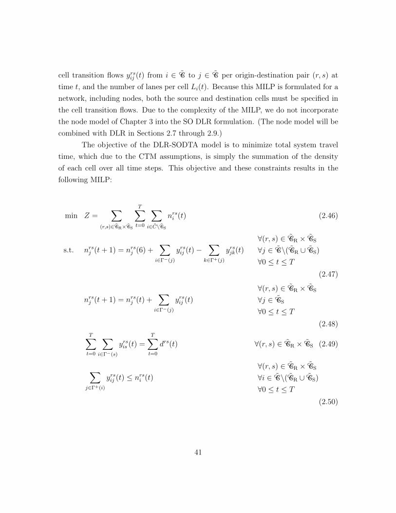
cell transition flows yrsij (t) from i ∈ C to j ∈ C per origin-destination pair (r, s) at
time t, and the number of lanes per cell Li(t). Because this MILP is formulated for a
network, including nodes, both the source and destination cells must be specified in
the cell transition flows. Due to the complexity of the MILP, we do not incorporate
the node model of Chapter 3 into the SO DLR formulation. (The node model will be
combined with DLR in Sections 2.7 through 2.9.)
The objective of the DLR-SODTA model is to minimize total system travel
time, which due to the CTM assumptions, is simply the summation of the density
of each cell over all time steps. This objective and these constraints results in the
following MILP:
min Z =∑
(r,s)∈ CR× CS
T∑t=0
∑i∈C\ CS
nrsi (t) (2.46)
s.t. nrsj (t+ 1) = nrsj (6) +∑
i∈Γ−(j)
yrsij (t)−∑
k∈Γ+(j)
yrsjk(t)
∀(r, s) ∈ CR × CS
∀j ∈ C\( CR ∪ CS)
∀0 ≤ t ≤ T
(2.47)
nrsj (t+ 1) = nrsj (t) +∑
i∈Γ−(j)
yrsij (t)
∀(r, s) ∈ CR × CS
∀j ∈ CS
∀0 ≤ t ≤ T
(2.48)
T∑t=0
∑i∈Γ−(s)
yrsis (t) =T∑t=0
drs(t) ∀(r, s) ∈ CR × CS (2.49)
∑j∈Γ+(i)
yrsij (t) ≤ nrsi (t)
∀(r, s) ∈ CR × CS
∀i ∈ C\( CR ∪ CS)
∀0 ≤ t ≤ T
(2.50)
41

∑r∈ CR
∑s∈ CS
w
ufnrsj (t) +
∑i∈Γ−(j)
yrsij (t)
≤ w
ufNjLj(t)
∀j ∈ C\( CR ∪ CS)
∀0 ≤ t ≤ T
(2.51)∑r∈ CR
∑s∈ CS
∑i∈Γ−(j)
yrsij (t) ≤ Qj(t)Lj(t)∀j ∈ C\( CR ∪ CS)
∀0 ≤ t ≤ T
(2.52)∑r∈ CR
∑s∈ CS
∑i∈Γ−(j)
yrsij (t) ≤ Qi(t)Li(t)∀i ∈ C\( CR ∪ CS)
∀0 ≤ t ≤ T
(2.53)
nrsr (t+ 1)− nrsr (t) +∑
j∈Γ+(r)
yrsrj (t) = drs(t)
∀(r, s) ∈ CR × CS
∀r ∈ CR
∀0 ≤ t ≤ T
(2.54)
nrsi (0) = 0
∀(r, s) ∈ CR × CS
∀(i, j) ∈ E
∀0 ≤ t ≤ T
(2.55)
yrsij (0) = 0
∀(r, s) ∈ CR × CS
∀(i, j) ∈ E
∀0 ≤ t ≤ T
(2.56)
yrsij (t) ≥ 0
∀(r, s) ∈ CR × CS
∀(i, j) ∈ E
∀0 ≤ t ≤ T
(2.57)
Li(t+ 1) ≥ Li(t)− 1∀i ∈ C
∀0 ≤ t ≤ T(2.58)
42

Li(t+ 1) ≤ Li(t) + 1∀i ∈ C
∀0 ≤ t ≤ T(2.59)
Li+1(t+ 1) ≥ Li(t)− 1∀i ∈ C
∀0 ≤ t ≤ T(2.60)
Li+1(t+ 1) ≤ Li(t) + 1∀i ∈ C
∀0 ≤ t ≤ T(2.61)
Li(t) + L←−i(t) ≤ `i
∀(i,←−i ∈ P
)∀0 ≤ t ≤ T
(2.62)
Li(t) ≥ 0∀i ∈ C
∀0 ≤ t ≤ T(2.63)
Constraints (2.47) through (2.54) define the cell transition flows. Constraints (2.50),
(2.51), and (2.52) have been modified from the original multi-destination CTM linear
programming model to account for the explicit representation of multiple lanes as a
decision variable. Constraints (2.58) through (2.61) bound the number of lanes that
can be reversed per time period, and constraint (2.62) defines the number of lanes
available to any pair of cells as `i, the total number of lanes available to both cells,
which is an input to the model. Note that all available lanes must be allocated during
all time periods, which will at times result in an arbitrary lane configuration.
2.6.2 Discussion
Let Z∗ be the optimal value of the objective function. Also, let Z = Z solved
with the additional constraints
Li(t) = Li ∀i ∈ C,∀0 ≤ t ≤ T (2.64)
for some Li’s satisfying La + Lb ≤ `a and Li ≥ 0 for all i ∈ C. Let Z∗ be the
optimal solution with corresponding flow and lane assignment(y∗, L
). Z∗ reduces to
solving the SO problem with a fixed lane configuration L. Clearly,(y∗, L
)is a feasible
solution to the original problem since the fixed configuration constraint (2.60) satisfies
43

Figure 2.4: (a) two link network and (b) cell representation
constraints (2.57) through (2.63). This analysis results in the following observation:
Proposition 7. Z∗ ≤ Z∗.
2.6.3 Demonstration and analysis
This section presents the SO DLR model results on a small corridor example
and a larger grid network. The DLR results are compared with the fixed-lane results.
The SO DLR problem was solved using the AMPL programming interface to the
CPLEX solver.
2.6.3.1 Two link demonstration
The SO DLR model is initially demonstrated on a simple two-link example in
order to closely analyze the relationship between dynamic lane allocation and dynamic
traffic demand patterns. Both links are of length 650 m with a free flow speed of 50
kph. Each link has two lanes with a capacity of 1800 vehicles/hour/lane. Figure 2.4
illustrates the demonstration network.
Using a time increment of 6 seconds, the each link is comprised of 8 cells with
N = 13.2 vehicles and Q = 3 vehicles. We examine four demand cases and compare
the DLR and fixed lane SODTA results. Demand case I is illustrated in Figure 2.5.
In case (I), the vehicle flow is much higher in one direction. In the traditional
fixed lane network, this situation will result in congested conditions. The SODTA
44

Figure 2.5: Demand case (I)
model considered 30 time steps, or 3 minutes of simulation. Demand for the first
ten time steps was assumed to be d13,14(t) = 10 vehicles and d16,15(t) = 3 vehicles
respectively. The demand follows a uniform departure time profile. The DLR model
resulted in a total travel time of 5166 seconds and 18 time increments for all vehicles
to exit the network. The fixed-lane approach was higher with a total travel time of
6834 seconds and 23 time-increments for all vehicles to exit.
Figure 2.6 shows a detailed representation of the lane configuration for pairs
of cells. Each vertical column represents the four lanes that are shared by a pair of
cells. The green shows that a lane is assigned to the first cell in the pair, while the
red represents a lane assignment to the second cell in the pair. For example, under
pair (13,15), all four lanes are assigned to cell 13 until time period 7. In demand case
I, the vehicle flow was unbalanced and therefore a majority of the lanes were able to
be utilized by the direction with a higher volume of flow. Also note that when there
is no vehicle demand for the cell or cell connector, the lane is assigned arbitrarily.
In the second case, the flow from both directions is more equal, as Figure
2.7 shows. This demand scenario is a common case for some congested network
corridors, even during peak hours. Demand for the first ten time steps was assumed
to be d13,14(t) = 9 vehicles and d16,15(t) = 5 vehicles.
In the fixed lane case, the model requires 16 time periods for all the flow to exit
the network while the DLR model requires 20 time-increments. The total travel time
in the fixed case was 7230 seconds and in the DLR case was 6756 seconds. Again, the
DLR model was able to reduce the total travel time. However, because there were
more vehicles from both directions, the reduction was not as great.
45

Figure 2.6: Lane configuration in demand case (I)
Figure 2.7: Balanced demand case (II–IV)
46

Figure 2.8: Lane configuration in demand case (III)
Demand case III examines the impact of time dependent demand, which an
important consideration for network operators. In this case, the total vehicle demand
is the same (90 vehicles/3 minutes) but the departure times are different. In this
scenario, the departure time are more spaced out and we assume d13,14(t) = 18 vehicles
for 0 ≤ t ≤ 24 and d16,15(t) = 10 vehicles for 60 ≤ t ≤ 84.
Both the fixed-lane and the DLR models require 25 time periods for all vehicles
to exit the network. However, the total travel time in the fixed case was 9084 seconds
and in the DLR case was 7488 seconds.
In addition, Figure 2.8 shows the detailed lane configuration in demand case
III. This demand scenario may be particularly conducive to dynamic lane allocation
because the first wave of demand from (13,14) had sufficient time to exit the network
before the second wave of demand from (16,15) entered the network.
Finally, in Table 2.1 we examine the peak demand case where the total demand
at each departure time is no longer uniform.
The total travel time for the fixed case is 8958, while the total travel time for
the SO DLR is 8718. The vehicles exited the network in 22 time-steps versus 18 time-
steps. Table 2.2 summarizes the results from the four demand cases. Additionally,
47

Table 2.1: Peak departure pattern demand
Time (14, 13) (16, 15)0 5 06 15 012 10 015 30 024 30 030 0 536 0 542 0 2048 0 1854 0 2
Total 90 50
Table 2.2: Summary of results for the two-link network
Total Departure # departure Fixed DLR DLR1
demand profile periods (s) (s) (s)I 100, 30 Uniform 10 7464 5796 5796II 90, 50 Uniform 10 7230 6756 6756III 90, 50 Uniform 5 9084 7488 8220IV 90, 50 Peak 5 8958 8718 8718
Table 2.2 presents the results for the case in which only two of the four lanes are
available to change directions as DLR1. This restriction would ensure that for all
time periods, each direction has at least one lane available which could be another
possible dynamic lane configuration.
Finally, we examined a 30 minute CTM simulation period, which is 300 time
steps. We loaded demand at the same rate (9 and 5 vehicles per time step respectively)
for 15 minutes, or 150 time steps. In this case, we placed a constraint that required
that there be at least one lane in each direction during all times periods (called DLR1).
There was a total of 1,350 vehicles between (13,14) and 750 between (16,15).
48

The DLR solution assigned 3 lanes to the direction with a greater volume
of vehicles and then switched to a 2 lanes in each direction configuration after 108
time increments. This relatively static assignment of lanes is expected because of
the uniform demand profile. If the demand were to arrive in more of a heavy-slow
pattern, we would expect there to be more changes in lane configuration as more
capacity was switched to the favored direction of travel.
The total travel time in the fixed case was 108.9 hours. The DLR model
reduced the travel time to 69.4 hours, which represented 36% of the travel time.
2.6.3.2 Grid network demonstration
Finally, this section presents the results for the SODLR model on a demon-
stration network with a grid structure and multiple origin-destination (OD) pairs. A
grid network results in additional paths available between each OD and may have a
significant impact on the performance of dynamic lane management. Furthermore,
the additional constraint (2.49) is necessary to ensure that the total demand between
each origin-destination is maintained.
Figure 2.9 shows the demonstration network with four zones (i.e., A, B, C,
D) that act as both origins and destinations. The OD pairs considered are A–D,
D–A, B–C, and C–B with a demand of 3300 vph, 300vph, 2700 vph, and 600 vph,
respectively. Links have identical properties and the same as the previous example
(i.e., two lanes available in the fixed case, a free flow speed of 50 kph and length of 650
m). In this network, we expect each OD pair to have three primary paths through
the network. The majority of demand will favor the most direct path through for
each OD, but as congestion increases, the paths on the outside links will become more
favorable.
We explore three different demand cases, similar to the two link example, and
each case has the same amount of total demand. Case I has a uniform departure
profile for ten departure time periods. Case II features a peak pattern of departure
over five time periods, while Case III has a more pronounced peak over three departure
time periods. The peak periods were chosen such that the departure time periods for
opposing OD pairs (i.e., A–D and D–A) were overlapping.
49

Figure 2.9: Grid network with four OD pairs
Table 2.3: Summary of results for the grid network demonstration
Demand Departure # departure Fixed DLR Decreasecase profile periods (min) (min)
Uniform 83, 8, 68, 15 10 238.74 200.95 15.8%Medium peak 83, 8, 68, 15 5 261.09 227.65 12.8%
High peak 83, 8, 68, 15 3 279.18 245.55 12.0%
Table 2.3 shows the results for the three demand cases on the grid shaped
demonstration network. The total demand is shown for OD pairs (A–D, D–A, B–C,
C–B). Table 2.3 shows the results for the fixed case where there are required to be
two lanes in each direction for all time periods and the SODLR case, where the lane
management can be optimized. In each case, the reduction in total travel time is
between 12–15%. That is a significant reduction for the relatively short simulation
period shown and suggests that DLR may be able to significantly reduce travel time.
However, for the case where the demand is overlapping in all directions, the reduction
in total travel time may be less.
50

2.7 Dynamic lane reversal on a single link
Section 2.6 presented a MILP formulation for the SO DLR problem. However,
in practice SO routing requires an impractical level of control over individual vehicles.
Even with AVs, travelers may be unwilling to follow proscribed routing. Furthermore,
the MILP is computationally intensive even for small networks. Therefore, it is
valuable to study DLR under the assumption of DUE behavior.
In this section we study the optimal DLR policy for a single link when sending
and receiving flows at the upstream and downstream ends are known. Although this
level of knowledge is still not completely realistic, this model is useful for developing
theory about the DLR problem. Furthermore, the lane manager may be able to
communicate with other lane and intersection managers across the city to acquire
sending and receiving flows for a limited time horizon. Section 2.8 studies DLR
policies for a single link with stochastic demand and downstream supply. Overall this
section focuses on policies from a single link perspective for computational tractability,
which is nevertheless demonstrated to improve total system travel time on a city
network in Section 2.9.
Without the additional constraints of the SO formulation, we again refer to
cell occupancies as ni(t) and cell transition flows as yi(t). Since we focus on a single
pair of links [a, b] and [b, a], recall that C is the set of cells on [a, b].
2.7.1 Motivation
We first motivate the discussion with a demonstration of the challenges in find-
ing an optimal DLR policy. A naıve approach might consider the objective of maxi-
mizing flow on a per time step basis, i.e. at t, choose lanes to max∑i∈C
(yi(t) + y←−
i(t)).
This objective is favorable because it exhibits the optimal substructure characteristic
for constructing a dynamic programming algorithm. However, consider two parallel
but opposite directional links with capacity 1200vph per lane, with 4 lanes between
them, 4 cells, and 4800vph demand in each direction for a limited time. Then the
lane configuration shown in Figure 2.10, maximizes flow initially but results in a bot-
tleneck in the middle of the link. Therefore, an optimal policy must consider future
51

Figure 2.10: Example of bottleneck lane configuration
evolution of flows.
2.7.2 Integer program
Because naıve methods for DLR policies may reduce flow, we formulate the
DLR problem for a single link as an IP. We then analyze this IP to derive some
theoretical results about the solution that inspire our heuristic in Section 2.8. To be
consistent with the cell notation, let cells 0 and←−−−−|C|+ 1 be source cells connected to
cells 1 and←−|C|, respectively. Because we assume demand and supply for the pair of
links under consideration are deterministic in this section, we model the upstream
and downstream links as point queues on source and sink cells. (This assumption
is relaxed in Section 2.8.) Let the number of vehicles entering the queues on 0 and←−−−−|C|+ 1 at time t be given by d0(t) and d←−−−|C|+1
(t). Then the queues of vehicles waiting
to enter the link at time T areT∑t=0
(d0(t)− y|C|(t, L)
)and
T∑t=0
(d←−−−|C|+1
(t)− y←−0
(t, L))
,
the differences between upstream demand and vehicles that entered the pair of links.
For the downstream ends, let cells |C| + 1 and←−0 be sink cells connected to
cells |C| and←−1 with receiving flows are R|C|+1(t) and R←−
0(t). Denote by y0(t) flow
entering cell 1 and by y←−−−|C|+1(t) flow entering cell
←−|C|. We consider the objective of
maximizing link throughput. Let L∗ be an optimal solution to the following IP:
max Z(L) =T∑t=0
ξt(y|C|(t, L) + y←−
1(t, L)
)(2.65)
52

s.t. yi(t, L) = min Si(t, L), Ri+1(t, L) ∀i,←−i ∈ C,∀t ∈ [0, T ]
Si(t, L) = min ni(t), QLi(t) ∀i,←−i ∈ C,∀t ∈ [0, T ]
Ri(t, L) = minQLi(t),
w
v(NLi(t)− ni(t))
∀i,←−i ∈ C,∀t ∈ [0, T ]
Li(t) + L←−i(t) ≤ ` ∀i ∈ C, ∀t ∈ [0, T ]
|Li(t)− Li(t+ 1)| ≤ 1 ∀i ∈ C, ∀t ∈ [0, T ]
|Li(t)− Li+1(t+ 1)| ≤ 1 ∀i ∈ C,∀t ∈ [0, T ]
Li(t) ∈ Z+ ∀i ∈ C,∀t ∈ [0, T ]
yi(t, L) ≥ 0 ∀i,←−i ∈ C,∀t ∈ [0, T ]
where ξ ∈ (0, 1] is a discount factor to discourage delayed throughput. ξ < 1 penalizes
delaying throughput to later time steps. ξ < 1 is necessary for analyses for which
T →∞, as ξ = 1 would result in Z(L)→∞ as T →∞.
Cell transition flows and vehicle movement may be specified for the single link
under consideration because it is assumed that vehicles will move forward if possible.
However, if multiple links were to be considered, the IP would have to include vehicle
route choice.
Z(L) as defined in the IP (2.65) maximizes discounted flow through the single
link under consideration. This IP does not directly apply to traffic networks because
of queue spillback. However, the DLR policy problem for a single link is sufficiently
complex to require heuristics when used with DTA. Solving the IP for a network
would introduce additional complexity in the form of route choice and intersection
conflicts. Therefore, we restrict our attention to flow on a single link. In Section
2.9.3, we show that the single link heuristic yields significant improvements for a city
network.
Proposition 8. The IP (2.65) has at least one feasible solution if for all cells i ∈ C,
(i) Li(0) + L←−i(0) ≤ `
(ii) |Li+1(0)− Li(0)| ≤ 1
(iii) |L←−−i+1
(0)− L←−i(0)| ≤ 1
53

(iv) NLi(0) ≥ ni(0)
(v) NL←−i(0) ≥ n←−
i(0)
Proof. From Proposition 6, there exists a solution satisfying the DLR constraints on
the number of lanes at each cell-time for t ≥ 0. The feasibility of flow propagation
constraints follows from CTM.
The conditions for Proposition 8 correspond to the constraints of the IP (2.65)
at t = 0.
Although solving the IP (2.65) yields the optimal DLR policy for a single link,
it is not sufficient for network analyses. The single-link model does not consider queue
spillback effects because demand waiting to enter the link is modeled as point queues.
Furthermore, solving this IP for every link in a city network is not tractable, especially
when UE route choice is taken into consideration. Therefore, the remainder of this
section develops structure and intuition about the single-link IP. This structure is
used to construct an effective heuristic in Section 2.8.
2.7.3 Bottlenecks
This section further explores the creation of bottlenecks on the links by al-
lowing y0(t) + y←−−−|C|+1(t) > Q` demand to enter in one time step. As seen in Section
4.1, bottlenecks can adversely affect the objective of maximizing total discounted
flow through the link. In Proposition 9, we prove that creating a bottleneck is not
necessary for optimality.
Intuitively, total flow between any pair of parallel opposing cells is restricted by
the capacity and the number of lanes. Lemmas 1 and 2 formally prove this intuition,
and are used in the proof of Proposition 9.
Lemma 1. For all L ∈ LT and i ∈ C, yi(t, L) + y←−i(t, L) ≤ Q`.
Proof. Since yi(t, L) ≤ QLi(t) and y←−−i+1
(t, L) ≤ QL←−i(t), and from constraint (2.40),
yi(t, L) + y←−−i+1
(t, L) ≤ QLi(t) +QL←−i(t) ≤ Q`.
Lemma 2. For all L ∈ LT and i ∈ C, yi(t, L) + y←−−i+1
(t, L) ≤ Q`.
54

𝑦𝑖 𝑡 ≤ 𝑄𝐿𝑖 𝑡
𝑦𝑖 𝑡 ≤ 𝑄𝐿𝑖 𝑡
𝐿𝑖 𝑡
𝐿𝑖 𝑡
Figure 2.11: Flow through a single cell
𝑦𝑖 𝑡 ≤ 𝑄𝐿𝑖 𝑡
𝑦𝑖+1 𝑡 ≤ 𝑄𝐿𝑖 𝑡
𝐿𝑖
𝐿𝑖
𝐿𝑖+1
𝐿𝑖+1
Figure 2.12: Flow between a pair of cells
Proof. yi(t, L) ≤ QLi(t) and y←−−i+1
(t, L) ≤ QL←−i(t), but Li(t)+L←−
i(t) ≤ ` by constraint
(2.40). Therefore yi(t, L) + y←−−i+1
(t, L) ≤ QLi(t) +QL←−i(t) ≤ Q`.
Lemmas 1 and 2 state that total flow through a cell or between a pair of cells
in any one time step is limited to Q` because only ` lanes are available at a single
cell, illustrated in Figures 2.11 and 2.12, respectively. These results are used as the
basis for a general result about bottlenecks:
Proposition 9. Suppose that there exists an i ∈ C, j ≥ i, t such that yi(t, L∗) +
y←−j
(t, L∗) ≥ Q`. Then there exists an L′ ∈ LT with Z(L′) ≥ Z(L∗) and yi(t, L′) +
y←−j
(t, L′) ≤ Q`.
Proof. By induction on j− i. The proof is split into two cases: whether the difference
between i and j is even or odd.
Basis: j = i: by Lemma 1, flow through cell i is limited to Q`, thereby limiting
the future reward. j = i + 1: by Lemma 2, flow through cell i is limited to Q`,
thereby limiting the future reward.
55

Inductive step: Suppose j − i = n+ 1 (with n+ 1 ≥ 2). If yi(t, L∗) + y←−
j(t, L∗) > Q`,
then such an L′ exists by the inductive hypothesis applied at i+ 1,←−−−j − 1, t+ 1 (with
(j − 1)− (i+ 1) = n− 1).
Proposition 9 notes that if in L∗, two cells i and j at some time t have yi(t, L∗)+
y←−j
(t, L∗) > Q`, then some alternate policy L′ with yi(t, L′) + y←−
j(t, L′) ≤ Q` is also
optimal. Note that Proposition 9 applies for flow entering in opposite directions at
the time step, or for flow entering and flow already on the link. Therefore, Proposition
9 allows restrictions to be placed on the solution. For instance, in a pair of links with
4 lanes total, if it is optimal to assign 3 lanes to one direction in one time step and
entering flow exceeds 2Q, then it is optimal to assign 3 lanes to succeeding cells in
succeeding time steps to allow that flow to reach the end of the link.
2.7.4 Partial lane reversal
A major modeling decision in the above formulation is deciding lane direction
at the cell level, as opposed to the entire link. From Proposition 9, L1(t)+L←−|C|(t) > `
is not necessary for optimality. However, the opposite, where L1(t) + L←−|C|(t) < `,
could be beneficial to add additional turning lanes for exiting vehicles. To prevent
queue spillback for one turning movement from interfering with another until vehicles
exit, additional turning lanes longer than one cell could also improve flow. Although
lane reversals to improve short-term flow at the end of the link may not be optimal in
the long term, a discount factor of ξ < 1 encourages giving preference to exiting flow
due to the total discount of at least ξ|C| from the minimum time required to traverse
the link. Proposition 10 demonstrates that under certain conditions, a partial lane
reversal on cell |C| will improve the total discounted flow through the link. Symmetric
conditions apply to cell←−1 . These conditions are likely to occur at some time step
for many networks.
Proposition 10. If
(i) L∗|C|(t) ≤ L∗|C|(t− 1)
56

(ii)t∑
t′=0
d←−−−|C|+1(t)−
t−1∑t′=0
y←−−−|C|+1(t, L∗) ≤ Q
(L∗←−|C|
(t)− 1)
(iii) n←−|C|(t) ≤ Q(L∗←−|C|
(t)− 1)
(iv) n|C|(t, L∗) ≥ R|C|+1(t) > QL∗|C|(t)
(v) ξ < 1
then there exists an L′ ∈ LT with Z(L′) > Z(L∗).
Proof. Construct L′ as follows: L′i(t) = L∗i (t) and L′←−i(t) = L∗←−
i(t) for all i ∈ C and
t′ ∈ [0, t], except that L′←−|C|
(t) = L∗←−|C|
(t) − 1 and L′|C|(t) = L∗|C|(t) + 1. L′ is feasible
because of condition (i). Because of conditions (ii) and (iii) removing a lane from←−|C| does not restrict flow. Then for all i ∈ C and t′ ∈ [0, t], yi(t
′, L′) ≥ yi(t′, L∗)
and y←−i(t′, L′) ≥ y←−
i(t′, L∗). Furthermore, because of condition (iv), y|C|(t, L
′) >
y|C|(t, L∗). From condition (v), Z(L′) > Z(L∗).
Condition (i) in Proposition 10 ensures feasibility of adding a lane to |C|.Conditions (ii) and (iii) state that the numbers of vehicles in cells
←−−−−|C|+ 1 and
←−|C|
are sufficiently small that removing a lane from←−|C| will not obstruct flow. Finally,
condition (iv) states that the number of vehicles in |C| and the receiving flow on
|C| + 1 are greater than the capacity allocation from L∗, and thus adding a lane
to |C| will result in y|C|(t, L′) > y|C|(t, L
∗) when moving flow later is discounted in
accordance with condition (v). Condition (v) is necessary because it rewards reducing
delays, and adding a temporary extra turning lane is designed to reduce delays. With
ξ = 1, there might be no difference in objective from providing an extra turning lane
instead of forcing some vehicles to wait until the next time step.
2.7.5 Stability
Because the objective function in the IP (2.65) maximizes discounted flow
through the link, the optimal solution without a discount has a superstable property:
if any policy prevents queues from growing to infinity as T → ∞, then L∗ is such a
57

policy. First, we bound the queue lengths when L∗ is used. Let d(L) be the sum of
the queue lengths at the end of the time horizon, T , for policy L ∈ LT . Then
d(L) =T∑t=0
((d0(t)− y|C|(t, L)
)+(d←−−−|C|+1
(t)− y←−1
(t, L)))
(2.66)
Proposition 11. Let T ≥ 0, L ∈ LT , and ξ = 1. Then d(L) ≥ d(L∗).
Proof. From the objective function with ξ = 1,
T∑t=0
((y|C|(t, L
∗))
+(y←−
1(t, L∗)
))≥
T∑t=0
((y|C|(t, L)
)+(y←−
1(t, L)
))(2.67)
Therefore
d(L∗) =T∑t=0
((d0(t)− y|C|(t, L∗)
)+(d←−−−|C|+1
(t)− y←−1
(t, L∗)))
≤T∑t=0
((d0(t)− y|C|(t, L)
)+(d←−−−|C|+1
(t)− y←−1
(t, L)))
= d(L) (2.68)
Denote by (LT ) = (LT : LT ∈ LT , T ∈ Z+) a sequence of feasible policies where
every T ∈ Z+ is mapped to a policy LT ∈ LT . Similarly, denote by (L∗T ) a sequence of
optimal policies to the IP (2.65). For any sequence of policies (LT ), the resulting re-
maining queue lengths also form a sequence(d(LT )
). Obviously,
(d(LT )
)is bounded
below as d(LT ) ≥ 0 for any LT ∈ LT . However(d(LT )
)may not be bounded above
(and if it is bounded, the sequence may not converge). Nevertheless, we can use such
sequences to establish the superstability of (L∗T ).
Proposition 12. Let ξ = 1, and suppose that there exists a sequence of feasible
policies (LT ) and a ζ ∈ R+ such that(d(LT )
)is bounded by ζ (i.e. for all T ∈ Z+,
d(LT ) ≤ ζ). Then(d(L∗T )
)is also bounded by ζ.
58

Proof. For any T , d(L∗T ) ≤ d(LT ) by Proposition 11. Since d(LT ) ≤ ζ, d(L∗T ) ≤ ζ.
Proposition 12 states the superstable property: if some sequence of feasible policies
(LT ) results in bounded queue lengths, then (L∗T ) also has bounded queue lengths.
However, these stability results require that ξ = 1, i.e. that delaying exiting flow has
no effect on the objective, as long as flow exits before T . This result is due to the
relationship between the queue length and the objective function. When a discount
is used, inequality (2.67) becomes
T∑t=0
((ξty|C|(t, L
∗))
+(ξty←−
1(t, L∗)
))≥
T∑t=0
((ξty|C|(t, L)
)+(ξty←−
1(t, L)
))(2.69)
which only yields
T∑t=0
((d−1(t)− ξty|C|(t, L∗)
)+(d←−−−|C|+1
(t)− ξty←−1
(t, L∗)))
≤T∑t=0
((d−1(t)− ξty|C|(t, L)
)+(d←−−−|C|+1
(t)− ξty←−1
(t, L)))
(2.70)
Inequality (2.70) shows how a policy L∗ for ξ < 1 may not be optimal for bounding
queue length. As a counterexample, consider a scenario in which the policy may shift
lanes to cells 0 through |C| to allow more vehicles on the link to exit, or shift lanes to
cells←−|C| through
←−0 to allow more queued vehicles to enter (and exit |C| time steps
later). For sufficiently small ξ, the optimal policy will prioritize vehicles already on
the link because they can exit sooner, although this policy may result in a longer
queue for entering cell←−|C| at the end of the time horizon.
Although ξ = 1 is necessary for superstability to hold, ξ < 1 does not neces-
sarily prevent the optimal policy from bounding queues for some demand scenarios.
However, L∗ cannot be guaranteed to bound queues if ξ < 1. The choice of discount
factor is similar to the capacity-delay tradeoff for traffic signals, where longer cycle
lengths increase both capacity and delay. As ξ increases, the optimal policy prioritizes
capacity more than delay. ξ = 1 maximizes capacity but also removes any penalty
59

for delaying vehicles. On the other hand, as discussed in Section 2.7.4, ξ < 1 is a
necessary condition for adding extra turning lanes to increase the objective function
in some scenarios.
The stability discussion also demonstrates some weaknesses of the IP approach.
Besides requiring perfect information about demand, the IP also is solved for a fixed,
finite time horizon. The solution results in a policy optimized for a specific demand
scenario. Because it is an IP, minor changes to the demand could result in major
changes to the optimal policy. In the next section, we study DLR with stochastic
demand as a Markov decision process (MDP). The resulting heuristic policy is more
robust and tractable than the solution to this IP.
2.8 Dynamic lane reversal with stochastic demand
Although perfect information about demand yields ideal scenarios and cor-
responding theoretical results, in reality acquiring perfect information for arbitrary
time horizons (such as the entire AM peak) requires knowledge of both vehicle route
choice and departure times. Changes in either would potentially require solving the
entire model again for some subinterval of time. Therefore, developing a DLR policy
for stochastic supply and demand is also valuable. From the perspective of the link
manager at time t, we assume that the change in demand d0(t), d←−−−|C|+1(t) and supply
R|C|+1(t), R←−0
(t) for the next time step are known, but future demand and supply
are given by stochastic processes. In general, upstream sending flow at t + 1 is not
independent of upstream sending flow at t because vehicles that do not enter at t will
wait for the next time step. Similarly, if downstream receiving flows are limited by
congestion at time t, there is a higher probability they will be limited by congestion
at time t + 1. Since all vehicles are in communication with the link manager, we
assume that for all i ∈ C, ni(t) and n←−i(t) are deterministic. Therefore, we consider
the following infinite-horizon MDP with state space S, control space U, and one-step
rewards g(t):
• The state at time t is the cell occupancies and number of lanes. Therefore, the
60

state space is
S= [0, N`]2|C| × Z2+ × [0, `]2|C| (2.71)
The integer 2|C|-vectors of [0, N`]2|C| are the possible combinations of cell occu-
pancies because N` is the maximum occupancy of any single cell, and there are
|C| cells in each direction. Z2+ is the possible lengths of the queues of vehicles
waiting to enter the links. The integer 2|C|-vectors of [0, `]2|C| are the possible
lane configurations.
• The control is how many lanes are assigned to each cell. Therefore,
U⊂ [0, `]2|C| (2.72)
The control space is limited by constraints (2.40) through (2.45) to ensure that
vehicles do not change lanes more than once per time step, and that each cell
has enough lanes that vehicles in the cell have sufficient physical space.
• The one-step rewards are given by the objective function to the IP:
g(t) = y|C|(t, L) + y←−1
(t, L) (2.73)
where transition flows y|C|(t, L) and y←−1
(t, L) are determined by equation (2.34).
• The state transitions are determined by entering demand and transition flows.
Entering demand is d0(t) and d←−−−|C|+1(t). Transition flows are described by equa-
tion (2.34) for CTM. The transition flows are affected by the number of lanes
assigned to each cell.
• The objective is to find a policy L∗ of lane assignments that maximizes the
long-run expected reward.
With a countable state space and finite action space, the MDP has an op-
timal stationary policy. Unfortunately, solving this MDP is fairly difficult. Due to
the simulation-based CTM state, solving it analytically encounters similar issues to
solving DTA with CTM analytically. Computational methods for solving MDPs,
61

based on dynamic programming, are polynomial in the state space. However, the
state space is intracatble due to the curse of dimensionality. For instance, a typical
0.5 mile, 4 lane pair of links with free flow speed 30 miles per hour and jam density
120 vehicles per mile has 10 cells in each direction, and each cell could contain up
to 24 vehicles. This portion of the state alone results in a state space of 4.01 × 1027
elements. Choosing out of 5 possible lane configurations (0 through 4) per cell in one
direction results in a further orthogonal 9.8× 10⁶ possibilities.
Based on the complexity, it would be ideal to derive theoretical results for the
MDP similar to the analyses in Section 2.7. Propositions 8 and 11 can be extended
to the MDP with similar proofs. However, Proposition 9 does not have a direct
counterpart in the stochastic case. Consider a pair of links with 2 lanes in each
direction, 900 vph capacity per lane, expected 900 vph demand in each direction,
time step of ∆t, and ξ = 1. If, due to randomness, 3600∆t demand in direction 1
appears at time t, based on expected future demand assigning 3 lanes to direction 1
at time t is a maximum throughput policy. If at times t + 1 through t + 5, 3600∆t
demand also appears in direction 2, to maximize throughput a bottleneck on the link
should be created in direction 1 as the potential reward in direction 2 is greater.
2.8.1 Heuristic algorithm
Therefore, instead of attempting to solve this MDP computationally, we use
the analytical structure developed in Section 2.7 to inspire a saturation-based heuris-
tic. Hausknecht et al. (2011b) briefly discuss a theorem on DLR with respect to
saturation, but it assumes stationary, constant flow and does not include downstream
receiving flow limitations. We use their method as a heuristic for the stochastic de-
mand, CTM model to determine expected saturation levels for two links [a, b] and
[b, a]. At time t, we first determine the number of lanes per cell, then propagate flow.
To simplify the possible actions, we choose two modes of control. First, all but
the last cell is assigned the same number of lanes, formally cells 1 through |C| − 1
and cells←−|C| through
←−2 . Although Proposition 9 may not hold in its most general
sense, allowing more than Q` of flow to enter in one time step still cannot increase
the reward. Furthermore, we add the restriction that each direction must always
62

have at least one lane, even if no flow is presently using it. This restriction prevents
flow in one direction from being completely obstructed due to high demand in the
other direction. In most practical scenarios, it is unlikely for one direction to have
completely zero demand.
2.8.1.1 Overall lane direction
Inspired by Theorem 1 of Hausknecht et al. (2011b), this heuristic estimates
the difference between demand and capacity for each direction. If demand exceeds
capacity in one direction, and the other direction has unused capacity, then it may
be beneficial to reverse one lane. Since the number of lanes is integer, we choose to
reverse a lane only if shifting Q capacity from one direction to the other is expected
to improve flow. Formally, define σλ(t) as the saturation estimation for direction
λ ∈ 1, 2, where the direction index is assigned arbitrarily. σλ(t) > 0 and σλ(t) < 0
indicate over- and under-saturation, respectively. To avoid confusion with Li(t), let
lλ(t) represent the number of lanes in direction λ. The initial condition is l1(t− 1) +
l2(t− 1) = `. Set
σ1(t) = min
∑
1≤i≤|C|ni(t) +
∑0≤t′≤T
E[S−1(t+ t′)],∑0≤t′≤T
E[R|C|+1(t+ t′)]
−Ql1(t− 1)T (2.74)
and
σ2(t) = min
∑
1≤i≤|C|n←−i(t) +
∑0≤t′≤T
E[S←−−−|C|+1(t+ t′)],∑
0≤t′≤TE[R←−−1
(t+ t′)]
−Ql2(t− 1)T (2.75)
T defines how far ahead into the future the heuristic considers when estimating
saturation. A low value of T will not allow all vehicles to exit, and will result in
the heuristic being highly reactive to specific realizations of supply and demand.
Therefore we recommend T be at least the number of cells in the link. On the
other hand, a high value of T might prevent the heuristic from reacting optimally to
63

dynamic congestion.
The minimum term in σλ(t) is the possible expected throughput of the link,
accounting for expected upstream sending flow and constraints of expected down-
stream receiving flow. The subtracted term is the maximum throughput possible
over T using lanes lλ(t− 1).
If σ1(t) > (Q+ σ2(t))+ and lane constraints (2.40) through (2.45) allow it, set
l1(t) = l1(t − 1) + 1, where (·)+ = max0, ·. Similarly, if σ2(t) > (Q+ σ1(t))+ and
lane constraints (2.40) through (2.45) allow it, set l2(t) = l2(t − 1) + 1. These two
conditions cannot both be true because if σ1(t) > (Q+ σ2(t))+ then σ2(t) < σ1(t),
and vice versa.
2.8.1.2 Additional turning bays
In addition, the last cell can be assigned extra turning lanes to allow more flow
to exit, based on Proposition 10. We refer to the number of lanes at the start and
end cells of direction 1 as l11(t) and l|C|1 (t), respectively. For direction 2, the number
of lanes at the start and end cells are l←−|C|2 (t) and l
←−1
2 (t), respectively. Initially, set
l11(t) = l|C|1 (t) = l1(t) and l
←−|C|2 (t) = l
←−1
2 (t) = l2(t). For direction 1, if l+ 1(t) ≤ l1(t− 1)
(to satisfy at most 1 additional lane per time step), set
σ′11 = minn|C|(t), Q (l1(t) + 1) , R|C|+1(t)
−min
n|C|(t), Ql1(t), R|C|+1(t)
(2.76)
and
σ′21 = minS←−−−|C|+1
(t), Ql2(t)−min
S←−−−|C|+1
(t), Q (l2(t)− 1)
(2.77)
σ′11 is the difference in flow for the cases of l|C|1 (t) = l1(t)+1 and l
|C|1 (t) = l1(t),
and σ′21 is similarly the difference in flow for the cases of l←−|C|2 (t) = l2(t) − 1 and
l←−|C|2 (t) = l2(t). If the improvement is sufficient, i.e. if σ′11 > 0 and σ′11 > σ′21, then
set l|C|1 (t) = l1(t) + 1 and l
←−|C|2 (t) = l2(t)− 1. An analogous operation is performed for
direction 2.
64

Flow propagation
Calculate cell transition flows
and move vehicles
Have all vehicles exited?
Dynamic lane reversal
Determine lane directions for
each pair of parallel cells
no
yes
End simulation
Start
Figure 2.13: Cell transmission model simulation with dynamic lane reversal
2.8.1.3 Simulation algorithm
This heuristic is part of the Simulate procedure in Algorithm 1. Every time
step, we use the above heuristic to determine the number of lanes in each direction for
each pair of parallel cells using equations (2.74) through (2.77). Then, we calculate
transition flows using equations (2.34) through (2.36), and propagate flow according
to equation (2.33). We repeat this calculation each time step until all vehicles have
exited. The simulation is illustrated in Figure 2.13. DLR adds the step of deciding
lane directions before propagating flow. The remainder of the simulation is the same
as conventional CTM.
65

2.8.2 Demonstration
To demonstrate the effectiveness of the above heuristic, we performed a suite
of tests on a single pair of links with varying combinations of stationary demand.
Each link was 0.4 miles long, had 2 lanes, 1200 vph capacity, 30 mph free flow speed,
15 mph backwards wave speed, and arrivals were Poisson each time step based on
demand. A time step of 6 seconds was used for CTM (as used by Ziliaskopoulos
and Waller, 2000), and the lookahead parameter T was set to 40 time steps. Due
to randomness in the demand, each scenario was simulated 100 times for 1 hour,
and average results are presented. Figure 2.14 graphs the difference in throughput
between DLR and a fixed lane configuration of 2 lanes in each direction.
Figure 2.14 demonstrates that in asymmetric demand scenarios where the
total demand is less than the total link capacity including lanes in both directions,
the DLR heuristic tends to improve over the fixed base lane configuration. Although
these results are not surprising, theyare important for several reasons.
First, although contraflow lanes would achieve similar results in some of the
demand scenarios considered, they are difficult to implement due to human drivers.
When AV intersection controllers are in use, DLR may be implemented on every link,
and this experiment demonstrates some of the benefits of doing so.
Second, this heuristic responds particularly well to scenarios in which one di-
rection is slightly oversaturated and the other is slightly undersaturated, but reversing
a lane would not improve the total flow. For example, consider a link with 4 lanes,
with 1200vph capacity per lane, and with demand of 2700vph in one direction and
1500vph in the other. With 2 lanes in each direction, 300vph of demand will not be
served, which is also true for a 3–1 lane configuration. DLR allows frequent changing
between 2–2 and 3–1 configurations, allowing that additional 300vph to use the link.
The proposed heuristic switches automatically based on the queues of vehicles waiting
to enter.
Finally, this DLR heuristic was not observed to perform significantly worse
than a fixed lane configuration. In several demand scenarios the average throughput of
DLR was slightly worse than that of fixed lanes. However, the decrease was two orders
66

0
600
1200
1800
2400
3000
3600
-200
0
200
400
600
800
1000
1200
0 300 600 900 1200 1500 1800 2100 2400 2700 3000 3300 3600 Dem
and
2 (
vph
)
Ad
dit
ion
al f
low
fro
m D
LR (
vph
)
Demand 1 (vph)
-200-0 0-200 200-400 400-600 600-800 800-1000 1000-1200
Figure 2.14: Change in total throughput from DLR heuristic
of magnitude less than the potential improvement. Overall, these results suggest that
while this heuristic may not be the optimal policy for DLR, in many cases it improves
over a fixed lane configuration, and it will probably not be much worse. Therefore,
this heuristic is worth consideration on larger networks.
2.9 Dynamic lane reversal on networks
Although the heuristic developed in Section 2.8 proved effective on single link
bottlenecks with stationary demand, the ultimate goal is to apply DLR to larger
67

networks with the additional variables of intersection constraints and DUE routing.
Therefore, we incorporate the heuristic into DTA, presented in Algorithm 1.
Algorithm 1 Dynamic lane reversal in dynamic traffic assignment
1: procedure Initialization2: for each link [a, b] do3: if there exists a link [b, a] with the same free flow speed and length then4: Pair [a, b] and [b, a] together for DLR5: end if6: end for7: for m = 1 to M do8: Add 1
Mof unassigned vehicles to the network
9: Path-generation(1)10: Simulate11: end for12: end procedure13:
14: procedure Method of successive averages15: for m = 1 to M do16: Path-generation( 1
m)
17: Simulate18: end for19: end procedure20:
21: procedure Path-generation(λ)22: for each ODT (r, s, t), find shortest path π∗rst do23: for each vehicle v traveling from r to s departing within t do24: Assign v to π∗rst with probability λ25: end for26: end for27: end procedure
2.9.1 Determining expected sending and receiving flows
The saturation definitions in equations (2.74) and (2.75) use expected demand,
which depends on traveler route choice. To determine this endogenously, each link
68

Algorithm 1 Dynamic lane reversal in dynamic traffic assignment (continued)
28: procedure Simulate29: for t = 0 to ∞ do30: for each link [a, b] do31: if [a, b] is paired with [b, a] then32: Determine lane assignment for [a, b] and [b, a]33: end if34: end for35: for each link [a, b] do36: Propagate flow through [a, b]37: Update expected sending and receiving flows38: end for39: end for40: end procedure
stores expected sending and receiving flows per assignment interval (AST). In DTA,
ASTs are used to reduce the computational complexity of routing demand. Typi-
cally, each iteration a single shortest path is found for every origin-destination-AST
(ODT) tuple. For DLR, we also use ASTs as the aggregation level for expected send-
ing and receiving flows because it corresponds to the path assignment aggregation.
Because changes in route choice affect expected sending and receiving flows, each it-
eration, the expected values per link are updated based on average observations from
the simulation. Average upstream sending flows for link [a, b] are calculated as the
average number of vehicles wanting to enter [a, b]. (For general networks, this calcu-
lation requires disaggregation of sending flows of upstream links by destination link).
Receiving flows are more difficult to calculate because of intersection constraints on
crossing flow. Instead, we used the average exiting flow as the expected receiving flow
for the heuristic. For congested links this estimate is accurate because exiting flow is
bounded by receiving flows. For uncongested links, DLR is not necessary anyways.
2.9.2 Dynamic traffic assignment algorithm
The first step of Algorithm 1 is to determine which links can be paired for
DLR. We paired together any links [a, b] and [b, a] with the same length and free
69

flow speed. In practice, some pairs of opposite and parallel links are separated by a
median or divider. We assume that for AVs, such dividers are not necessary for safety
purposes. We also did not have specific data on which pairs of links had dividers or
not. However, if such dividers are used in practice, they would prevent DLR from
being applied.
For the first iteration, expected sending and receiving flows are not known, so a
partial demand initialization (Levin et al., 2015b) is used to both improve convergence
and provide initial inputs to DLR. DLR is embedded in the simulation step of DTA,
as illustrated by Figure 2.13. Every time step, lane assignments are chosen using
the heuristic in Section 2.8. After each simulation, expected sending and receiving
flows are recorded. This definition of DLR uses values from only the last iteration.
However, because the number of vehicles moved continuously decreases through MSA,
the change in the DLR policy gradually decreases as well.
2.9.3 City network results
To demonstrate the tractability and effectiveness of our proposed heuristic, we
tested it on the downtown Austin network, shown in Figure 2.15, which has 62836
trips over 2 hours, 171 zones, 546 intersections, and 1247 links in the AM peak. CTM
was used with a time step of 6 seconds and an AST duration of 15 minutes. DLR was
implemented on all pairs of parallel and opposite direction links with the same speed
and length. As much of the network is a downtown grid, DLR was implemented on
most links in the network. Because DLR is most applicable when all vehicles are AVs,
the conflict region model (Levin and Boyles, 2015b) with FCFS priority was used for
intersections. To fully explore the impact of our proposed DLR heuristic, we did not
include the capacity improvements from reduced reaction times in these results. In
Chapter 4 we will study the effects of combining DLR, pressure-based intersection
control, and capacity improvements from AVs.
The demand is completely deterministic. However, because route choice changes
through the process of solving for dynamic user equilibrium, determining the demand
for individual links in the network would require forward simulation. Due to the
computational cost of simulating many possible lane direction scenarios, it is easier
70

Figure 2.15: Downtown Austin network
71

0.00%
1.00%
2.00%
3.00%
4.00%
5.00%
6.00%
7.00%
8.00%
1 3 5 7 9 11 13 15 17
Co
st g
ap a
s p
erc
en
t o
f tS
TT
Iteration
Figure 2.16: Convergence of dynamic lane reversal on downtown Austin
to model link-specific demand as a random variable.
To demonstrate our DLR heuristic, we solved DTA for two scenarios: current
(fixed) lane configuration, and DLR. We then compared the travel times at UE for
both scenarios. To avoid skewing results by different levels of convergence, both
scenarios were solved to the same cost gap of 2% of total system travel time.
Convergence of DTA with DLR is demonstrated in Figure 2.16. The partial
demand initialization resulted in a relatively small initial gap. Around 4–5%, the
cost gap percent oscillated, which was probably due in part to DLR. However, after
iteration 9 the cost gap steadily decreased, suggesting it found a local equilibrium.
With the addition of DLR, DTA required 8.16 minutes to solve on an Intel Xeon
CPU at 3.07 GHz. These computation times make it tractable for study on large city
networks.
Our heuristic was developed for a single link, and the results in Section 2.8.2
show its effectiveness. However, the network level introduces route choice and queue
spillback, neither of which are considered in our analysis of DLR policy for single
link flow. The results presented here could be further improved by including network
effects.
72

Table 2.4: Total system travel time
Scenario TSTT (hr)Fixed lanes 8420.966
DLR heuristic 6588.828
Table 2.4 shows the total system travel time (TSTT) for both fixed lanes and
when the DLR heuristic was used. The DLR heuristic resulted in an improvement
of 21.8% over fixed lanes. This experiment demonstrates the potential benefits of
using DLR during peak hour demand. As this experiment is the AM peak, most of
the demand is headed towards the downtown region, shown in Figure 2. The extra
capacity afforded by DLR helps alleviate the congestion caused by the asymmetric
use of right-of-way. On average, distance traveled by the same vehicle was observed
to decrease by 23.9% when DLR was used. This result suggests that greater capacity
on shorter distance routes increased their utility in DUE routing.
Figure 2.17 shows the average improvement in travel time from DLR for vehi-
cles at different departure times. Vehicles departing later receive the greatest benefit
because those vehicles experience a more congested network, and DLR alleviates
much of the congestion. Overall, these results demonstrate that the DLR heuristic is
effective at improving efficiency in congested large city networks.
This particular test network contains both freeways on the east and west
boundaries and a detailed downtown region. (Some links in downtown are two-way,
while others are one-way and do not have a counterpart for DLR). Vehicles traveling
shorter distances are more likely to take arterials or the downtown grid, whereas ve-
hicles traveling longer distances are more likely to take freeways and downtown roads
due to the geometry of the network. Figure 2.18 demonstrates that vehicles traveling
between 1–2 miles and 5+ miles in the fixed lane configuration experienced similar re-
ductions in travel times. This result suggests that the DLR heuristic is more effective
for arterials than restricted access freeways because vehicles traveling longer distances
have a greater potential for reductions in travel time. This effectiveness could be due
to the limited number of lanes on exit ramps; DLR would not be able to add extra
73

0
50
100
150
200
250
0 900 1800 2700 3600 4500 5400 6300 7200
Re
du
ctio
n in
tra
vel t
ime
(s)
Simulation time
Figure 2.17: Average reduction in travel time at different assignment intervals
lane capacity to these ramps. As with the VISTA DTA simulator (Ziliaskopoulos and
Waller, 2000), the queueing model allows queues for these ramps to block entire cells.
Surprisingly, vehicles traveling 3–4 miles experienced a significantly lower reduction in
travel time. This observation suggests further study into the effects of DLR on DUE
routing could be useful. However, regardless of the distance, vehicles experienced
average reductions in travel time, which suggests this heuristic consistently improves
over the fixed lane configuration.
2.10 Conclusions
To provide a framework for studying the effects of AVs on city networks, this
section developed a shared road DTA model for human and autonomous vehicles. A
multiclass CTM was presented for vehicles traveling at the same speed with capacity
and backwards wave speed a function of class proportions. A collision avoidance car-
following model incorporating vehicle reaction time iwas used to predict how reduced
reaction times might increase capacity and backwards wave speed. These models are
generalized to an arbitrary number of classes because different AVs may be certified
74

0
20
40
60
80
100
120
140
160
0 1 2 3 4 5
Re
du
ctio
n in
tra
vel t
ime
fro
m D
LR (
s)
Distance traveled
Figure 2.18: Average reduction in travel time from DLR with respect to vehiclemiles traveled.The ith bin corresponds to vehicles traveling between i and (i+ 1) miles.
for different reaction times. These models also use continuous flow so that DTA
models built on continuous flows may incorporate these multiclass predictions.
We also developed a cell transmission model with variable number of lanes in
space and time consistent with the kinematic wave theory of traffic flow to model DLR.
We explored and developed a MILP model based on the multi-destination SODTA (Li
et al., 2003) that propagates traffic using the cell transmission model. The number
of lanes in each cell is explicitly considered as a decision variable, allowing for real
time network design in response to time-varying travel demand. Results illustrate the
importance of accounting for time-varying demand profiles when exploring the DLR
concept. However, due to the integer representation of lanes, this approach will face
significant computation challenges when using traditional optimization techniques.
The model presented here motivates the possibility of DLR, but a number of simpli-
fications were necessary, which could be the subject of future research. This model
could also be compared with contraflow lanes (reversing the direction of a lane for
the entire peak period) to determine the benefits of DLR over existing technology.
75

We then focused on a single link and considered the scenarios of known and
stochastic demand. When demand is known, we demonstrated that a solution algo-
rithm should consider future demand and receiving flows and formulated DLR as an
IP. We derived theoretical results about the optimal solution(s), noting that using
lane reversals to create a bottleneck on a link is never necessary for optimality when
demand is known, and proving that the optimal solution will stabilize queues if they
can be stabilized.
Because demand is often not known perfectly at arbitrary times in the future,
we formulated the DLR problem with stochastic demand as a MDP. The MDP was
analytically difficult to solve because it is built on a DTA model, and the curse
of dimensionality led to computational intractability. Nevertheless, we developed a
heuristic based on saturation estimates that was demonstrated to work well on a single
bottleneck link at various combinations of stationary demand. We then presented an
algorithm for using the heuristic in dynamic traffic assignment, and tested it on a
city network. DTA converged to an equilibrium and resulted in a 21.8% reduction in
TSTT.
76

3 Node model of reservation-based
intersection control
3.1 Introduction
The computer precision and communications abilities of AVs admit new inter-
section behaviors with the potential to improve traffic flow, such as reservation-based
control (Dresner and Stone, 2004, 2006b). Run by a computerized intersection man-
ager, reservations divides each intersection into a grid of space-time tiles to monitor
conflicts. Vehicles must communicate a request to occupy specific space-time tiles
to the intersection manager, which accepts reservations under the condition that two
vehicles cannot occupy the same space-time tile. Fajardo et al. (2011) and Li et al.
(2013) demonstrated that reservations can reduce delay over optimized traffic signals.
Since intersection managers are forced to reject many reservations to prevent
conflicts, an important question is how to decide which reservations to reject. Early
studies used a FCFS policy in which reservations are prioritized according to the
time of the request. Later studies considered priority for emergency vehicles (Dresner
and Stone, 2006a) and using auctions to determine priority (Schepperle and Bohm,
2007, 2008; Vasirani and Ossowski, 2012; Carlino et al., 2013). Shahidi et al. (2011)
also considered batching reservations to improve over FCFS. However, the range of
strategies for deciding which vehicles move when potential conflicts exist is arbitrarily
large. Previous work has focused on priority-based resolution of conflicting reservation
requests. Depending on the strategy, it may be optimal for the intersection manager to
aggregate requests, then choose a non-conflicting subset according to some objective.
77

To study such strategies, a more general model is necessary.
One major issue with reservations is the computational tractability of simulat-
ing vehicle movements through the grid of tiles. Smaller tiles results in greater inter-
section utilization but correspondingly greater computational requirements. Reser-
vations in its original form is therefore intractable for solving DTA. The problem of
modeling reservations in DTA has been addressed by two recent papers: Zhu and
Ukkusuri (2015) proposed a conflict point simplification, which focuses only on the
intersections between turning movement paths in the grid of tiles. However, as we
will discuss in Section 3.3.1, intersections with a large number of lanes and turning
movements would have a correspondingly large number of conflict points, limiting the
computational efficiency.
Alternately, Levin and Boyles (2015b) proposed to aggregate the tiles into
larger conflict regions constrained by capacity. While effective for DTA, they did not
fully justify using conflict regions instead of conflict points or tiles. In addition, their
priority function for resolving conflicts does not directly correspond to an objective
function for the intersection policy. Therefore, this chapter improves over the work
of Levin and Boyles (2015b) through two objectives:
1. Provide justification for using the conflict region model to approximate reser-
vations. To accomplish this justification, we begin by formulating the conflict
point simplification (Zhu and Ukkusuri, 2015) as an IP for DTA. By aggre-
gating conflict points for tractability we derive an IP for the conflict region
model (Levin and Boyles, 2015b).
2. Create more system-efficient policies for reservation-based control. The fairness-
based FCFS policy is potentially suboptimal for typical policy goals such as
maximizing intersection flow. The unspecified objective function of the conflict
region IP admits arbitrary system policies for moving vehicles across the inter-
section. We propose a polynomial-time heuristic for this NP-hard IP and study
pressure-based objective functions that are effective at reducing total travel time
on a city network.
78

3.1.1 Contributions
The contributions of this chapter are as follows: we present an IP for the
conflict point simplification of the reservation-based model. For tractability, we ag-
gregate conflict points into conflict regions and derive a corresponding IP. Because the
objective is unspecified, this formulation results in a reservations model that admits
arbitrary strategies for moving vehicles across a reservation-controlled intersection.
This IP may also be used as a framework for DTA models of reservations. Since this
IP is NP-hard, we propose a greedy polynomial-time heuristic. Finally, we demon-
strate the potential utility of the IP — and our heuristic — through an objective
function that increases intersection efficiency on a city network.
3.1.2 Organization
The remainder of this chapter is organized as follows: First, Section 3.2 dis-
cusses previous literature on reservations, reservation policies, and backpressure and
P0. Then, Section 3.3 derives the conflict region model as an IP and Section 3.4
presents a greedy heuristic. Section 3.5 explores scenarios in which signals perform
better than reservations. Section 3.6 adapts backpressure and P0 for reservations,
and Section 3.7 presents results. We conclude in Section 3.8.
3.2 Literature review
The tile-based reservation protocol proposed by Dresner and Stone (2004,
2006b) operates through an intersection manager agent communicating wirelessly
with individual vehicles. The intersection manager divides the intersection into a
grid of space-time tiles, illustrated in Figure 3.1. Vehicles request a reservation from
the intersection manager, which simulates the vehicle’s desired path through the grid.
If no conflicts occur, the reservation may be accepted. Otherwise, the reservation of
one or more of the conflicting vehicles must be rejected. Vehicles must know their
arrival time at the intersection to request to enter the intersection at a specific time.
79

(a) Accepted (b) Rejected
Figure 3.1: Tile-based reservation protocol (Fajardo et al., 2011)
3.2.1 First-come-first-serve policy
A major question for reservation controls is which vehicle’s reservation should
be accepted when requests conflict. Dresner and Stone (2004, 2006b) suggested prior-
itizing on a FCFS basis for fairness. Studies comparing reservations with signals (Fa-
jardo et al., 2011; Li et al., 2013) focused on FCFS and found that FCFS could reduce
delays beyond optimized signals. However, as we will show in Section 3.5, in some
situations signals will perform better than FCFS-based reservations.
FCFS is a fairness-based method for accepting reservations that has been used
in most previous studies. When a vehicle requests a reservation, the intersection man-
ager accepts it if it does not conflict with previously accepted reservations. Otherwise,
it is rejected, and the intersection manager advises a later possible time (Fajardo et al.,
2011). Equivalently, the vehicle is delayed until it can safely make its desired turning
movement.
Although simple, the definition of FCFS results in some important properties
that are exploited in the paradoxes of reservation-based control in Section 3.5:
1. Vehicles are prioritized by when they first requested a reservation, independent
of external costs imposed on other vehicles. For instance, vehicles making left
80

and right turns impose different conflict separation requirements on intersection
traffic, but the type of turning movement does not affect FCFS priority. This
disconnect is exploited in Section 3.5.1.1.
2. Reservation request time may not be the same as time spent queued or other in-
tuitive measures. Vehicles cannot request a reservation unless they can execute
it. Therefore, vehicles in a queue, or at the back of a platoon, may not request
a reservation until they are able to enter the intersection. A road with more
lanes may correspondingly obtain a greater share of the intersection capacity
because the vehicle at the front of each lane can request a reservation. Also,
vehicles on a long low-traffic road may be able to request a reservation long be-
fore reaching the intersection, because in free-flow conditions their arrival time
at the intersection is known. This timing is exploited in Section 3.5.1.2.
3. If one vehicle’s request is accepted, other requests that do not conflict may also
be accepted. This combining of requests may result in vehicles moving in an
order that is different from the order of their reservation requests.
For instance, in the four-approach intersection in Figure 3.2, suppose there are 3
vehicles, each at the front of their lane: vehicle 1 requests to move north-south
through the intersection, vehicle 2 requests to move east-west, and vehicle 3
requests to move south-north (in that order). Vehicle 1’s reservation is accepted
due to priority. Vehicle 2’s reservation is rejected due to conflict with vehicle 1.
Vehicle 3’s reservation is then accepted because it does not conflict with vehicle
1. Vehicles 1 and 3 move at the same time, and vehicle 2 moves after.
3.2.2 Alternative reservation policies
The question of vehicle priority admits a wide range of potential policies.
Dresner and Stone (2006a) suggested giving higher priority to emergency vehicles,
although other traffic already typically yields the right-of-way to them. Shahidi et al.
(2011) proposed batching reservations to avoid the fairness attribute of FCFS from
dominating intersection use. Studies by Schepperle and Bohm (2007, 2008), Vasirani
81

2
1
3
Figure 3.2: Conflict region representation of four-way intersection
and Ossowski (2010, 2012), and Carlino et al. (2013) demonstrated that using auc-
tions for priority can in some cases reduce delay beyond that of FCFS for all vehicles,
not just high-bidding vehicles. Intersection auctions are an interesting development
for the area of congestion pricing because intersection pricing opens up the possibility
of tolling every link, which can potentially yield SO routing under UE behavior (Beck-
mann et al., 1956). Auctions also introduce the possibility of vehicles paying other
vehicles for the delays caused to them. From the perspective of traffic management
policy, one significant result from the work on auctions is demonstrating that optimal
strategies for reservations have yet to be identified. Modeling and improving on such
strategies is one goal of this chapter.
One major potential issue for reservations is that its communication complex-
ity restricts usage by human drivers. Since it is likely that AVs will not be in exclusive
use for many decades, extensions that allow humans to use reservation-based controls
have been studied. Dresner and Stone (2006a, 2007) proposed periodically providing
a green light to specific lanes or links for human drivers. Qian et al. (2014) extended
the reservation system to human-driven and semi-autonomous vehicles under certain
assumptions about path and car-following behaviors, and Conde Bento et al. (2013)
82

proposed reserving larger sections of the intersection for human-driven vehicles. Such
interventions should be compatible with general reservations strategies by requiring
occasional allowances for non-autonomous vehicles.
Optimizing reservations is further complicated by the effects of UE routing,
which can produce system inefficiencies such as the well-known Braess (1968) para-
dox. Network studies of reservations have been complicated by its computational
requirements. Previous network models with reservations have not included traffic
assignment, and were limited in size (Hausknecht et al., 2011a) or forced to reduce
the number of tiles for computational tractability at the cost of intersection effi-
ciency (Carlino et al., 2012). Zhu and Ukkusuri (2015) developed a LP for flow
through the conflict point model, albeit with some further restrictions on conflicting
flow. Levin and Boyles (2015b) developed the conflict region model of reservations
for simulation-based dynamic traffic assignment (SBDTA), which was shown to be
tractable for solving SBDTA on large city networks. For a more general model of
reservation-based intersection control, we combine the conflict point and conflict re-
gion approaches by developing a discrete vehicle-based IP for the conflict point model
and transforming its feasible region to achieve the conflict region model.
3.2.3 Pressure-based control
This section first discusses the backpressure policy for communications net-
works. Then, we review the P0 policy for maximizing intersection throughput with
UE route choice.
3.2.3.1 Backpressure policy
The backpressure policy originates from studies of multihop communication
networks. Such networks typically involve packets traveling from some origin node to
some destination node with unspecified routing. The seminal paper of Tassiulas and
Ephremides (1992) is concerned with developing a policy that is stable for the largest
possible region of demands. A stable policy is a policy in which customer queues
at each node remain bounded. Using a queueing model, Tassiulas and Ephremides
83

(1992) proposed a maximum throughput policy based on queue pressure — the dif-
ference between upstream and downstream queues. They proved that choosing the
combination of packets that maximized the relieved pressure at each node resulted in
maximum stability. Route choice was determined by the system at each node based
on downstream queue lengths.
As the work of Tassiulas and Ephremides (1992) is focused on communication
routing, the assumptions and modeling are not standard to traffic literature. First,
they modeled links as point queues without a free flow travel time. This assumption
was made because in electronic communications, the transmission speed is typically
fast (possibly the speed of light) relative to node processing speeds. Therefore, their
packets are modeled as traversing a link in one time step. This travel behavior may be
applied to traffic by reversing the nodes and links: vehicles take relatively little time
to traverse an intersection compared with the typical link travel time, and intersection
controls determine intersection access. However, in traffic networks, queues require
physical space. Later extensions to finite-buffer queues (Giaccone et al., 2007; Le
et al., 2012) required a minimum buffer size, which cannot be guaranteed for arbitrary
roads. As demonstrated by Daganzo (1998), queue spillback with DUE route choice
can create significant congestion issues. Furthermore, traffic queues place first-in-first-
out (FIFO) restrictions on vehicle movement, whereas in communication networks
the order of service may be arbitrary. Finally, Tassiulas and Ephremides (1992)
adaptively determine route choice in response to queue lengths, whereas vehicles
typically choose routes individually, resulting in DUE behavior. Although tolling can
encourage a system-optimal route choice, the route choices specified by backpressure
could change every time step, and current tolling models have not considered changing
route choice at such high frequencies.
Nevertheless, several papers have applied the backpressure policy to traffic in-
tersections. Zhang et al. (2012a) proposed a pressure-based algorithm for intersection
control that determined the probability of a driver choosing a specific turning move-
ment based on the difference in the upstream and downstream link queue lengths.
This behavior is challenging to resolve with DUE route choice, but Zhang et al.
(2012a) modeled adaptive route choice on a hyperpath, similar to some stochastic
84

DUE models. Gregoire et al. (2014) applied the pressure idea more conventionally
with respect to route choice by using the difference between upstream and downstream
queue lengths to choose which signal phase to activate. Wongpiromsarn et al. (2014)
also included lack of route control in their adaptation of the pressure-based algorithm
to signal control, and provided an analytical treatment similar to that of Tassiulas
and Ephremides (1992). Under the assumption of infinite queue capacities, they were
able to show that their pressure-based policy maximized throughput. However, prac-
tical limitations such as link length require careful choice of the pressure function
to avoid queue spillback. Therefore, Xiao et al. (2014) proposed a pressure-releasing
policy that accounts for finite queue capacities. Nonetheless, to more canonically
apply the pressure-based routing they assumed that each turning movement has a
separate queue, which is often not realistic.
A major limitation on signal control is the clearance intervals necessary to sep-
arate phases for human drivers. Some demand scenarios could result in frequent phase
switching as the pressure relieved by one phase makes another phase have relatively
higher pressure, and it does not appear that previous work on using backpressure poli-
cies to activate signal phases included lost time penalties in their models. Frequent
phase switching for signalized intersections would result in considerable time lost to
clearance intervals. Therefore, we apply the backpressure policy to reservation-based
control, which does not require clearance intervals and has much greater flexibility in
vehicle movements.
3.2.3.2 P0 traffic signal policy
In contrast to the communication network pressure-based approach, the P0
signal control policy by Smith (1980) is designed for traffic intersection control with
UE route choice. Smith (1979) demonstrated that Webster’s signal policy could sig-
nificantly reduce network capacity due to UE route choice, and Smith (1981) further
derived properties about signal policies that resulted in a consistent equilibrium. For
instance, Webster’s policy and a delay-minimizing policy induce route choice counter
to the objectives of the signal policy. This route choice behavior motivated the P0
policy of Smith (1980), which was also derived from traffic assignment principles later
85

discussed by Smith and Ghali (1990). The problem P0 addresses is how to allocate
green time to each signal phase. P0 uses the principle that low pressure phases re-
ceive no green time to avoid encouraging vehicles to switch to low capacity routes.
As specified by Smith and Ghali (1990), the pressure on a phase is the product of
saturation flow and link travel delay. This policy favors links with two properties:
1. Links with high saturation flow have a greater ability to service demand. Pro-
viding more green time to high saturation flow links will encourage drivers to
choose links that can better handle the demand.
2. Links with a high delay (due to unsatisfied flow) have a longer queue of demand
waiting to be serviced by the intersection.
Whereas P0 is capacity maximizing, follow-up work by Smith and Van Vuren (1993)
studied policies that are gradient, monotone, and/or capacity maximizing with respect
to the BPR cost function. Smith and Ghali (1990) also provided a method of modeling
P0 signal timing as a static traffic assignment problem. Meneguzzer (1997) provided
a review of papers considering signal timing and UE together. Liu and Smith (2015)
extended this work to a day-to-day bottleneck model and demonstrate that if the
delay formula is non-decreasing and the P0 policy is used for the signal control, then
flow swapping among pairs will achieve equilibrium. Overall, in contrast to the work
on backpressure, the work on the P0 signal policy is much more inclusive of UE route
choice effects, and we therefore also consider P0 for reservations.
3.3 Derivation of conflict region model
This section justifies the conflict region model by deriving it from the conflict
point model of reservations in two steps:
1. In Section 3.3.1, we present a conflict point IP for DTA. This formulation in-
volves replacing continuous time with discrete time steps. As is typical with
SBDTA, vehicles crossing the intersection are assumed to begin and complete
their turning movement within one time step. Therefore, we constrain conflict
points by capacity rather than occupancy.
86

2. Section 3.3.2 presents the conflict region IP by aggregating conflict points into
conflict regions for tractability.
3.3.1 Conflict point model for dynamic traffic assignment
The reservation control policy (Dresner and Stone, 2004) operates on a grid
of tiles in space-time. The tile conflict analysis of reservations may be simplified
through the definition of conflict points (Zhu and Ukkusuri, 2015). As illustrated in
Figure 3.3, the paths for any two turning movements (i, j) and (i′, j′) first intersect
at some point c. Ensuring adequate spacing at c for vehicles traveling from (i, j)
and (i′, j′) will guarantee that no conflict occurs at c or anywhere in the intersection
between vehicles moving from i to j and from i′ to j′. For vehicles uniform in physical
characteristics and acceleration behaviors, these conflict points are fixed. However,
in terms of practical implementation, tiles may be required instead of conflict points
to handle vehicles of different shapes and turning behaviors. Nevertheless, in many
DTA models physical uniformity of vehicles is assumed.
Previous work on reservations (Fajardo et al., 2011) studied tiles with width
as small as 0.25 meters to improve intersection efficiency. Assuming 3 meter wide
lanes, the intersection in Figure 3.3 requires 676 such tiles in space. With 3 turning
movements per link, and 4 links, there are a total of 12 paths through the intersection.
In the worst case, in which each turning movement conflicts with all movements from
other links, each turning movement has only 9 conflicts, for a total of 108 conflict
points. In general, for a rectangular intersection with ℵ lanes along the width and
i lanes along the height, the number of tiles is Θ (ℵi). Assuming vehicles are not
permitted to change lanes in the intersection, the number of turning movements is
O(ℵ + i), and thus the number of conflict points is O ((ℵ+ i)2). Therefore the
conflict point model scales worse than the tile model. However, as demonstrated
by the analysis of Figure 3.3, the conflict point model may be significantly more
efficient for small intersections. The conflict point model also admits mathematical
programming methods (Zhu and Ukkusuri, 2015).
In their conflict point LP, Zhu and Ukkusuri (2015) assume that vehicles can-
not simultaneously propagate through two conflicting lane movements. Depending
87

𝑖
𝑗
𝑖′ 𝑗′ 𝑐
Figure 3.3: Illustration of conflict points between turning movement paths.
on the magnitude of the time step, this assumption may or may not lead to over-
conservative estimates. For sufficiently large time steps allowing adequate spacing,
two vehicles from conflicting turning movements should be able to traverse a single
conflict point. That assumption is relaxed in this chapter through capacity constraints
on conflict points.
Let CP be the set of conflict points, and let yv(t) denote whether vehicle v
enters the intersection in time step t. Turning movements from different lanes of
the same link may encounter different conflict points as they follow different paths
through the intersection. Therefore, denote by Γ− and Γ+ the sets of incoming and
outgoing lanes, respectively, and let Γ−(v) be the incoming lane for vehicle v.
The sending flow is the number of vehicles that would move if there were no
intersection conflicts or constraints in the downstream link. Let Si(t) be the sending
flow for lane i and S(t) =⋃i∈Γ+
Si(t) be the total sending flow for the intersection in
time t. We assume that S(t) includes vehicle order.
In most SBDTA models, vehicles are assumed to begin and complete turning
movements within the same time step. Turning movements spanning multiple time
88

steps are normally not considered. Therefore, instead of constraining the arrival
times of individual vehicles at conflict points, we constrain the total flow through each
conflict point during each time step. This constraint is equivalent to a major difference
between micro-simulation and DTA: in car-following models, vehicles decelerate to
avoid colliding with the vehicle in front; in DTA, speed decreases as density increases
to model vehicle deceleration to avoid collisions.
The limitation on conflict point flow is a capacity-based restriction. Although
using this constraint reduces the power of the model to prevent intersection conflicts,
conflicting movements still constrain flow at an aggregate level consistent with SBDTA
flow models. Let δcv ∈ 0, 1 denote whether c ∈ πv, and let Qc be the capacity
of conflict point c. Vehicles from lane i require a spacing headway of 1Qc(i)
where
Qc(i) is the capacity reserved for vehicles from lane i moving through c. Then the
separation constraint is∑
v∈S(t)
δcv1
Qc(Γ−(v))≤ ∆t, where ∆t is the simulation time step.
This constraint may be written as∑
v∈S(t)
δcvQc
Qc(Γ−(v))≤ Qc∆t, which yields the capacity
reduction in Levin and Boyles (2015b). In addition, we add a receiving flow constraint
for all lanes j:∑
v∈S(t)
yv(t)δjv ≤ Rj(t), where δjv denotes whether v enters lane j.
For first-in-first-out (FIFO) movement, assume that SBDTA determines arrival
order for discrete vehicles. Let θ(v) be the time v arrives at the intersection, and let
Sv(t) = v′ ∈ SΓ−(v)(t) : θ(v) > θ(v′) (3.1)
be the set of vehicles that arrived at the intersection before v on the same lane. Then
all v′ ∈ Sv(t) must move before v due to FIFO, which may be written as
yv(t) ≤ 1−|Sv(t)| −
∑v′∈Sv(t)
yv′(t)
M(3.2)
If |SΓ−(v)(t)| −∑
v′∈Sv(t)
yv′(t) > 0 then at least one vehicle in front of v has not yet
moved, and the lane is blocked for v. These transformation result in the following IP.
Note that this program is for every time step t, so t is assumed fixed.
89

max Z(y(t)) (3.3)
s.t∑v∈S(t)
yv(t)δcv
Qc (Γ−(v))≤ ∆t ∀c ∈ CP (3.4)
∑v∈S(t)
yv(t)δjv ≤ Rj(t) ∀j ∈ Γ+ (3.5)
yv(t) ≤ 1−|Sv(t)| −
∑v′∈Sv(t)
yv′(t)
M∀c ∈ CP (3.6)
yv(t) ∈ 0, 1 ∀v ∈ S(t) (3.7)
where y(t) is the vector formed by the decision variables yv(t). Z(y(t)) is left unspec-
ified to admit arbitrary objectives.
3.3.2 Conflict region model
For computational efficiency, conflict points may be combined in the model into
conflict regions, illustrated in Figure 3.2. This combining could result in modeling a
conflict between two turning movements that do not intersect, but for a sufficiently
large conflict region it is likely that turning movements would intersect within it.
With the aggregation of conflict points into conflict regions, denoted by the set CR,
lanes may similarly be aggregated into links. Thus, from this point forward, Γ−(v)
and Γ+(v) refer to the incoming and outgoing links for vehicle v, respectively. Denote
by Li the number of lanes link i has. The number of lanes affects the FIFO constraint
because vehicles cannot enter the intersection unless they are at the front of a lane.
These modifications result in the following IP:
max Z(y(t)) (3.8)
s.t∑v∈S(t)
yv(t)δcv
Qc (Γ−(v))≤ ∆t ∀c ∈ CR (3.9)
90

yv(t) ≤ 1 +QΓ−(v)− 1
M∀v ∈ S(t) (3.10)∑
v∈S(t)
yv(t)δjv ≤ Rj(t) ∀j ∈ Γ+ (3.11)
yv(t) ∈ 0, 1 ∀v ∈ S(t) (3.12)
where
QΓ−(v)(v) =
Qi −∑
v∈Sv(t)
yv(t)
LΓ−(v) −
(|Sv(t)| −
∑v′∈Sv(t)
yv′(t)
)LΓ−(v)
(3.13)
Constraints (3.10) and (3.13) are the generalization of constraint (3.6) for multiple
lanes. When a vehicle blocks a lane due to a rejected reservation, the capacity for
vehicles behind is restricted. Lane-blocking is modeled by the function QΓ−(v)(v),
which is the remaining capacity for v as a function of whether vehicles ahead of
v moved through the intersection. The number of lanes available for use for v is
LΓ−(v) −
(|Sv(t)| −
∑v′∈Sv(t)
yv′(t)
). Qi −
∑v∈Sv(t)
yv(t) is the remaining capacity of the
link, which is reduced proportionally by the number of available lanes remaining.
When QΓ−(v)(v) ≥ 1, then yv(t) = 1 satisfies constraint (3.10). Note that QΓ−(v)(v) <
0 is possible in a sufficiently large queue. If LΓ−(v) or more vehicles in front of v have
not moved, then QΓ−(v)(v) ≤ 0, and v cannot enter the intersection. Nevertheless,
this IP always has a feasible solution. Let Y(t) be the set of feasible solutions to the
conflict region IP for time t.
Proposition 13. Y(t) 6= ∅.
Proof. Consider y(t) = 0. Rj(t) ≥ 0 and Qc∆t ≥ 0 , so constraints (3.11) and (3.12)
are satisfied. 1+QΓ− (v)−1
M≥ 0 so constraint (3.9) is satisfied. Therefore 0 ∈ Y(t).
91

3.4 Discussion
The purpose of this section is to discuss the use of the conflict region IP
(Section 3.3.2) in DTA. We begin by discussing the IP in the context of generic DTA
intersection models in Section 3.4.1, and derive some analytical results in the process.
3.4.1 Intersection modeling in dynamic traffic assignment
As an intersection model for DTA, it is relevant to study the conflict region IP
in equations (3.8) through (3.12) in the context of the requirements for generic DTA
intersection models described by Tampere et al. (2011):
1. general applicability
2. maximizing flows
3. non-negativity
4. conservation of vehicles
5. satisfying demand and supply constraints
6. obeying conservation of turning fractions
As stated, the conflict region IP satisfies all requirements except the invariance prin-
ciple. We show that the algorithm of Levin and Boyles (2015b), which satisfies the
invariance principle, creates a feasible solution for the IP, and in Section 3.4.2 we
present a heuristic for the general IP based on that algorithm.
For general applicability, we assume, as with Levin and Boyles (2015b), that
in the absence of other flow, flow between any (i, j) ∈ Γ−×Γ+ is constrained only by
sending and receiving flows. Let Qi be the capacity of link i; if Qi = Qj, then flow of
Qi should saturate the conflict region. This conflict region capacity behavior can be
satisfied by choosing
Qc = max(i,j)∈Γ−×Γ+:c∈πij
minQi, Qj (3.14)
92

where πij is the set of conflict regions flow from i to j will pass through. With
Qc (Γ−(v)) = Qi, then flow of Qi∆t through any conflict region c will result in equality
on constraint (3.9) because Qc
QiQi∆t = Qc∆t. Constraint (3.9) can then be written as
∑v∈S(t)
yv(t)δcv
Qc
QΓ−(v)
≤ Qc∆t ∀c ∈ CR (3.15)
Tampere et al. (2011) note that DTA intersection models should maximize
flow as drivers will move whenever possible. In a reservation-based context, vehicles
may be prevented from moving even if it is possible for them to move. However, it is
reasonable to assume that many practical intersection strategies will allow a vehicle
to move if its reservation request does not conflict with the reservation of another
vehicle and the downstream link has sufficient space. To achieve this behavior, the
objective function in (3.8) should satisfy the following:
Property 1. For any y(t),y′(t) ∈ Y(t), if for all v ∈ S(t) y′v(t) ≥ yv(t) and there
exists a v ∈ S(t) with y′v(t) > xv(t), then Z (y(t)) < Z (y′(t)).
Objective functions satisfying Property 1 yield the desired characteristic of the
solution to the conflict region IP:
Proposition 14. Let y∗(t) be an optimal solution to the conflict region IP and let
Z(·) satisfy Property 1. For any v ∈ S(t), if y∗v(t) = 0, form y′(t) with x′(t) = y∗(t)
except with y∗v(t) = 1. Then y′(t) is not feasible.
Proof. Suppose y′(t) is feasible. Since Z(·) satisfies Property 1, then Z (y′(t)) >
Z (y∗(t)), which contradicts y∗(t) being optimal.
Property 1 can be satisfied by Z (y(t)) = z · y(t) for some z > 0 or more
complex functions. It does not, however, require that the objective is to maximize
flow. For instance, FCFS can be modeled through the conflict region IP:
Proposition 15. The FCFS policy may be modeled through the IP in equations
(3.8) through (3.12). Specifically, there exists an objective function Z(·) satisfy-
ing the following: Let θ(v) be the reservation time of v. If, for all v1, v2 ∈ S(t),
93

v1 6= v2 =⇒ θ(v1) 6= θ(v2) and y∗(t) is chosen by FCFS, then for all y ∈ Y,
Z (y(t)) ≤ Z (y∗(t)).
Proof. By induction on |S(t)|. Sort S(t) by reservation request so that for any indices
i, j, if i < j then θ(vi) < θ(vj). Let t∗ be the reservation time of the last vehicle, and
let
Z (y(t)) =n∑i=1
M t∗−θ(vi)yvi(t) (3.16)
be the objective function. (This objective satisfies Property 1). We show that
n∑i=1
M t∗−θ(vi)y∗vi(t) ≥n∑i=1
M t∗−θ(vi)yvi(t) (3.17)
for all y(t) ∈ Y(t), for all 1 ≤ n ≤ |S|.
Base case: If v1 can move, then1∑i=1
M t∗−θ(vi)x∗vi(t) = M t∗−θ(v1) because FCFS priori-
tizes by request time, and M t∗−θ(v1) ≥1∑i=1
M t∗−θ(vi)y∗vi(t) for all y(t). If v1 is blocked,
then1∑i=1
M t∗−θ(vi)y∗vi(t) = 0 for all y(t).
Inductive step: If y∗vn+1= 1 or y∗vi = 0 for all 1 ≤ i ≤ n+ 1, then Proposition 15 holds
trivially. The remaining case is that y∗vn+1= 0 because of higher priority vehicle(s)
blocking its movement, i.e., if yvn+1 = 1 then for some vehicle i < n+ 1, yvi = 0.
M t∗−θ(vi) >∑
v∈SΓ−(v),tv>tvi
M t∗−θ(v) (3.18)
son+1∑j=i
M t∗−θ(vj)y∗vj >
n+1∑j=i
M t∗−θ(vj)y∗vj (3.19)
Then by the inductive hypothesis,n+1∑j=i
M t∗−θ(vj)y∗vj >n∑j=i
M t∗−θ(vj)y∗vj .
94
Proposition 15 proves that the oft-studied FCFS policy falls within the general
framework of the IP developed here. Setting M = ∆t should be sufficiently large,
although that may still result in impractically large numbers due to the exponential.
We prove in Proposition 18 that the polynomial-time algorithm of Levin and Boyles
(2015b) can find the optimal solution to the IP with FCFS objective (3.16).
The requirement of non-negativity (Tampere et al., 2011) is satisfied because
y(t) ≥ 0. Tracking discrete vehicles also satisfies conservation of flow and of turning
fractions. Demand constraints are satisfied by the implicit definition of the set of
sending flow, and supply constraints are explicitly satisfied by constraint (3.11).
The remaining requirement is the invariance principle, which essentially states
that the intersection flow should be invariant to the constraint on sending flow chang-
ing from the number of waiting vehicles to the link capacity. If |Si(t)| < Qi changes
to |S ′i(t)| = Qi, if one v ∈ S ′i − Si has a very high weight in the objective function,
the optimal solution to the conflict region IP may need to include v. Therefore, The
invariance principle may not be satisfied for general objective functions, although it
is for some objectives, including FCFS (Levin and Boyles, 2015b). The invariance
principle can be satisfied by an additional constraint (Tampere et al., 2011), or as a
corollary of alternate solution algorithms. For instance, the conflict region algorithm
of Levin and Boyles (2015b) satisfies the invariance principle. With a modification to
better model FIFO constraints, shown in Algorithm 2, the conflict region algorithm
finds a feasible solution to the conflict region IP. Specifically, Li tracks the number of
lanes blocked. These are combined in line 26 to satisfy constraint (3.13).
Proposition 16. The conflict region algorithm (Algorithm 2) produces a feasible
solution to the conflict region IP in equations (3.8) through (3.12).
Proof. For any v ∈ S(t), let V ′ be the set of vehicles considered before v in the loop
on line 11. If yv = 1, then v can move from i to j according to line 19. Line 14 results
in yi′j′ being the number of vehicles in v′ moving from i′ to j′. Consequently, line 26
requires that Rj ≥ 1 +∑v′∈V ′
δjv′yv′(t), so constraint (3.11) is satisfied. For all conflict
95

regions c that v passes through, line 30 of requires that
Qc ≥Qc
Qi
+∑v′∈V ′
δcv′yv′Qc
QΓ−(v′)(3.20)
satisfying constraint (3.9). Constraints (3.10) and (3.13) FIFO are satisfied because
vehicles either move through the intersection or block a lane (line 22). Blocked lanes
detract from outflow (line 26) and vehicles are considered for movement in FIFO
order. Finally, constraint (3.12) is satisfied because each vehicle is only considered
once in the loop on line 11.
The conflict region algorithm uses yij(t) to record flows between links i and j.
Throughout this dissertation, y is used to denote flows, whether they are specific to
a vehicle or to a cell or link.
Proposition 17. The running time of the conflict region algorithm (Algorithm 2) is
O(|CR||S(t)| log |S(t)|+ |Γ−||Γ+|
).
Proof. Initialization of V (lines 1 through 9) iterates through each vehicle in S(t)
once. Sorting V (line 10) is therefore O(|S(t)| log |S(t)|
). Initializing yij(t) requires
O(|Γ−||Γ+|
). Therefore initialization is O
(|S(t)| log |S(t)|+ |Γ−||Γ+|
).
The main loop (lines 11 through 24) iterates through each vehicle at most
once, thereby scaling with |S(t)|. It may add vehicles to V in sorted order, requiring
O(
log |S(t)|)
time to find the appropriate index. For each vehicle, the destination
link and the conflict regions it passes through is checked once for conflicts in the
canMove subroutine, which is O(|CR|
). If canMove returns true, the flow through
each conflict region is updated, which is also O(|CR|
). Therefore, the main loop is
O(|CR||S(t)| log |S(t)|
).
Although the conflict region algorithm produces a feasible solution in polyno-
mial time, it may not be optimal. It takes as input some priority f(·) to each vehicle,
and moves the highest priority vehicle able to enter the intersection. It does not con-
sider the value of moving a vehicle to allow vehicles behind to cross the intersection
sooner. However, for specific objective functions, such as FCFS, the priority function
will result in an optimal solution to the IP.
96

Algorithm 2 Conflict region algorithm
1: V := ∅2: for all i ∈ Γ− do3: Sort Si(t) by arrival time at i4: Remove first Li vehicles in Si(t) and add them to V5: Li := 06: for all j ∈ Γ+ do7: yij(t) := 08: end for9: end for
10: Sort V by f(v)11: for all v ∈ V do12: Let (i, j) be the turning movement of v13: if canMove(i, j) then14: yij(t) := yij(t) + 115: for all c ∈ CR
ij do
16: yc(t) := yc(t) + Qc
Qi
17: end for18: Remove first vehicle in Si(t) and add it to V in sorted order19: yv(t) := 120: else21: yv(t) := 022: Li := Li + 123: end if24: end for
97

Algorithm 2 Conflict region algorithm (continued)
25: function canMove(i ∈ Γ−, j ∈ Γ+)
26: if Rj(t)−∑i′∈Γ−
yi′j(t) < 1 or
(Qi −
∑j′∈Γ+
yij′(t)
)Li(t)−Li
Li(t)< 1 then
27: return false28: end if29: for all c ∈ CR
ij do
30: if Qc − yc(t) < Qc
Qithen
31: return false32: end if33: end for34: return true35: end function
Proposition 18. The conflict region algorithm, using reservation time as the prior-
itization (f(v) = θ(v)), produces an optimal solution for the FCFS policy.
Proof. From Proposition 16, the solution created by the conflict region algorithm
is feasible. Since vehicles cannot request a reservation unless they are not blocked
from entering the intersection, for any two vehicles v1, v2 ∈ S(t), θ(v1) < θ(v2) =⇒f(v1) ≤ f(v2). Therefore, if v1 ∈ V and v2 6∈ V , then (v1) ≤ f(v2). Once at the front
of the intersection, reservations are ordered by f(·) for consideration. Therefore, if
the reservation of v1 is rejected, there must be some v2 with f(v2) ≤ f(v1) blocking
the movement of v1, which is the definition of FCFS.
3.4.2 Heuristic
Solving general IPs is an NP-hard problem, and it is easy to construct scenarios
in which non-integer flows result in a greater objective value for the conflict region
IP. The computational requirements of solving the conflict region IP on a single
intersection per time step are well within the capabilities of current computers due to
the limitations on sending flows, and if arbitrary strategies were deployed in practice,
each intersection manager might solve the IP exactly. For modeling purposes, though,
solving many such IPs per simulation, and simulating the network many times to
98

solve for DUE, is computationally prohibitive. Certain objective functions can lead
to polynomial-time algorithms, such as FCFS. However, these limited cases are not
sufficient for arbitrary policy strategies. Therefore, in this section we propose a
polynomial-time greedy heuristic for objective functions of the form Z (y(t)) = z·y(t).
(The heuristic does not require that z > 0; because it is a greedy heuristic it will
move vehicles if their reservation request does not conflict with other vehicles.) Since
yv(t) ∈ 0, 1 for all v ∈ S(t), many potential policy strategies can be modeled by
this type of objective function.
The conflict region IP with objective z ·y(t) is similar to the class of problems
known as multiple-constraint knapsack (MCKS) problems (Kellerer et al.). In general,
MCKS problems on the set of sending flow are described as
max z · y(t) (3.21)
s.t. ωh · y(t) ≤ Ωh ∀1 ≤ h ≤ H (3.22)
yv(t) ∈ 0, 1 ∀v ∈ S(t) (3.23)
where vehicles moved are constrained by H resources. Each vehicle consumes some
ωhv ≥ 0 of resource h, with Ωh ≥ 0 available for use. The conflict region IP with
objective z ·y(t) is similar to this form as constraints (3.9) and (3.11) can be modeled
in the form of constraint (3.22). However, constraint (3.10) could have negative
coefficients on the decision variables.
Nevertheless, heuristics for MCKS problems have been studied in great detail,
and the similarities are useful for analyzing the conflict region IP. MCKS problems in
general are also NP-hard, and furthermore, no fully polynomial-time approximation
scheme exists (Kellerer et al.). The same proof that MCKS problems are NP-hard
may be applied to the conflict region IP where the number of lanes for each incoming
link are sufficiently large to be non-restrictive. Although pseudo-polynomial time al-
gorithms have been developed for the case in which ωh ∈ Z|S(t)|+ , since the coefficients
in constraint (3.9) may not be integral, the computational requirements of such al-
gorithms are likely still prohibitive. However, greedy heuristics for MCKS problems
have also been studied, and the FIFO constraint can easily be incorporated into a
99

greedy algorithm. The conflict region algorithm of Levin and Boyles (2015b), shown
in Algorithm 2, is in fact a greedy algorithm limited to a specific class of objective
functions. We generalize it into a heuristic for the conflict region IP with arbitrary
objective by including an efficiency ev, which is the value of moving vehicle v con-
sidering its resource consumption. Dobson (1982) studied the efficiency function of
ev =zv
H∑h=1
ωhv
Ωh
(3.24)
for the MCKS problem. We propose using vehicle priority f(v) = ev in the conflict
region algorithm, and greedily selecting the vehicle with the greatest efficiency from
the set of vehicles able to enter the intersection.
Due to the FIFO constraint on link queues, there exist scenarios in which this
heuristic is suboptimal, such as having a high weighted vehicle behind a low weighted
vehicle on a single lane link. For many practical objectives, such as maximum effi-
ciency, such disparity in vehicle weights is unlikely to occur. The results demonstrate
significant overall improvement when applying this heuristic to city networks for an
efficiency objective.
3.4.3 Reservations with mixed traffic
For shared road models, the intersection control policy is an important ques-
tion. With 100% human vehicles, optimized traffic signals are the best option avail-
able. With 100% AVs, reservations can reduce delay beyond that of optimized sig-
nals (Fajardo et al., 2011). The difficulty is the choice of intersection control policy
for shared roads. Dresner and Stone (2007) showed that reservations subsume traffic
signals because the signal essentially reserves parts of the intersection. They propose
link- and lane-cycling signals, where each link or lane successively receives full access
to the intersection, and vehicles in other links or lanes may reserve non-conflicting
paths. However, blocking out large portions of the intersection for a signal greatly
restricts reservations from other links due to the possibility of conflict, even when
most vehicles are AVs. As a result, combining signal phases with reservations may
100

not scale well when the proportion of AVs on the road becomes large. It is also an
open question whether link- or lane-cycling signals even outperform optimized traffic
signals.
Conde Bento et al. (2013) proposed the legacy early method for intelligent
traffic management (LEMITM). LEMITM reserves space-time for all possible turning
movements for non-AVs and also increases the safety margins to allow non-AVs to use
the reservation infrastructure. AVs still use conventional reservations, reserving only
the requested path. This protocol may be less efficient than traffic signals at small
proportions of AVs because of the extra space-time reserved to ensure safety. However,
as the proportion of AVs increases, LEMITM will devote less space-time to safety of
human vehicles because it is not constrained by protecting turning movements allowed
by traffic signals. As a result, LEMITM may scale at a higher rate. Therefore,
LEMITM is used in this dissertation to study how link and intersection capacity
scales with the proportion of AVs.
LEMITM makes two assumptions that we elaborate on here for the purposes
of describing the DTA model of LEMITM.
1. It separates vehicles into two groups: those that can establish digital com-
munications on reservation acceptance and adherence, and those that cannot.
The latter group consists of all non-AVs, although some AVs could conceivably
fall into that group as well. This assumption is reasonable in practice because
current technology can already determine whether a vehicle is waiting at the
intersection for actuated signals. Given that a vehicle is waiting, the inter-
section controller need only check whether the vehicle has established digital
communications, which can be determined if vehicles transmit their position to
the intersection controller along with reservation requests.
2. Due to the unpredictably of human behavior, the intersection controller must be
able to cancel granted reservations for AVs if a human is delayed in reacting to
permission to enter the intersection. Because this DTA model does not include
potential human errors and takes a more aggregate view of the intersection,
canceled reservations are not included in the model.
101

Most studies on reservation-based controls use micro-simulation and are there-
fore not computationally tractable for the number of simulations required to solve
DTA. Section 3.3.2 simplified reservations using the idea of larger conflict regions to
distribute intersection capacity and receiving flows to sending flows for compatibil-
ity with general SBDTA models. Although the conflict region model is designed for
arbitrary vehicle prioritization, LEMITM requires the intersection controller to re-
serve additional space and therefore make additional availability checks. This section
details the modifications to the conflict region algorithm to accommodate LEMITM.
The conflict region model is a polynomial-time algorithm performed at each
intersection each time step to determine intersection movement. Vehicle movement
is restricted by capacity of each conflict region it passes through during its turning
movement. The purpose of the conflict region algorithm (Algorithm 2) is to deter-
mine which vehicles move subject to the constraints of sending flow, receiving flow,
and conflict region capacity. This section focuses on the modifications necessary to
implement LEMITM.
The conflict region model requires discretized flow because of the priority func-
tion. For instance, Dresner and Stone (2004) proposed a first-come-first-serve priority,
and Dresner and Stone (2006a) suggested priority for emergency vehicles. Modeling
such prioritization functions with continuous flow is an open question, so discretized
flow is used instead. These prioritization functions are orthogonal to the LEMITM
control policy, although the communications required for more complex prioritization
functions such as auctions may be difficult for human drivers.
Two modifications to the control algorithm presented in Section 3.4 are re-
quired to implement LEMITM. First, for non-AVs, movement from i to j across the
intersection requires available capacity for all possible turning movements from i be-
cause the vehicle cannot communicate its destination to the intersection controller.
The set of conflict regions a vehicle leaving link i could pass through is ∪j′∈Γ+CRij′ .
It is not specific to j because for a human vehicle, the intersection manager does
not know the vehicle’s destination link. Therefore the intersection controller must
check whether all such turning movements have space available. Second, when such
a reservation is accepted, space for all possible turning movements from i must be
102

reserved. Denote by δAVv ∈ 0, 1 whether vehicle v is autonomous. The modified CR
model is formalized in Algorithm 3.
3.5 Paradoxes of first-come-first-served reservations
This section presents and characterizes several scenarios in which the use of
FCFS reservations results in greater delays than signals. We present three theoreti-
cal examples, including a temporarily saturated arterial-local road intersection to a
demonstration that replacing signals with reservations can result in infinite queuing.
Overall, these results demonstrate that while reservations perform better than traffic
signals in certain situations, network-based analyses are necessary to detect adverse
route choices before reservations can be used to replace signals entirely. In particu-
lar, asymmetric intersections (e.g. local road-arterial intersections) can cause several
potential issues with reservation controls.
3.5.1 Theoretical examples
This section presents three examples in which FCFS reservations are less effi-
cient than signals. First, we show that the fairness of FCFS can increase total vehicle
delay for asymmetric intersections. Next, we discuss how reservations can disrupt
platoon progression that is possible through optimally timing signals on a corridor.
Finally, we demonstrate that replacing a signal with a reservation control can lead to
arbitrarily large increases in queue size due to selfish route choice.
3.5.1.1 Greater total delay due to fairness
We first present a simple example of a temporarily oversaturated arterial-local
road intersection. Clearly, some vehicles must be delayed due to crossing conflicts.
We show that the fairness goal of FCFS results in greater total delay. Consider the
intersection A shown in Figure 3.4. As described in Table 3.1, links 1 and 2 form a
three-lane arterial with total capacity of 3600 vph. Links 3 and 4 form a one-lane
local road with capacity 1200 vph. Using a time step of 6 seconds, which is typical for
103

Algorithm 3 Conflict region algorithm for mixed AV/HV traffic
1: V := ∅2: for all i ∈ Γ− do3: Sort Si(t) by arrival time at i4: Remove first Li vehicles in Si(t) and add them to V5: Li := 06: for all j ∈ Γ+ do7: yij(t) := 08: end for9: end for
10: Sort V by f(v)11: for all v ∈ V do12: Let (i, j) be the turning movement of v13: if canMove(i, j) then14: yij(t) := yij(t) + 115: if δAV
v = 1 then16: for all c ∈ CR
ij do
17: yc(t) := yc(t) + Qc
Qij
18: end for19: else20: for all c ∈ ∪j′∈Γ+CR
ij′ do
21: yc(t) := yc(t) + Qc
Qij
22: end for23: end if24: Remove first vehicle in Si(t) and add it to V in sorted order25: yv(t) := 126: else27: yv(t) := 028: Li := Li + 129: end if30: end for
104

Algorithm 3 Conflict region algorithm for mixed AV/HV traffic (continued)
31: function canMove(i ∈ Γ−, j ∈ Γ+)
32: if Rj −∑i′∈Γ−
yi′j < 1 or
(Qi −
∑j′∈Γ+
yij′
)Li−Li
Li< 1 then
33: return false34: end if35: if δAV
v = 1 then36: for all c ∈ CR
ij do
37: if Qc − yc(t) < ufiτv+L
ufiτHV+L
Qc
Qijthen
38: return false39: end if40: end for41: else42: for all c ∈ ∪j′∈Γ+CR
ij′ do
43: if Qc − yc(t) < ufiτv+L
ufiτHV+L
Qc
Qijthen
44: return false45: end if46: end for47: end if48: return true49: end function
105

𝐴
1
2 4 3
Figure 3.4: Network for Section 3.5.1.1
Table 3.1: Link parameters for Section 3.5.1.1
Link Free flow Capacity (vph) Demand per time steptravel time(s) (first 2 time steps)
1, 2 18 3600 6 vehicles3, 4 18 1200 2 vehicles
the CTM (Daganzo, 1994, 1995a) used in simulation-based DTA, each time step six
vehicles can move from link 1 to link 2, or two vehicles from link 3 to link 4, or any
convex combination. Because the local road has lower capacity, moving one vehicle
from link 3 to link 4 reserves a capacity equivalent to moving three vehicles from link
1 to link 2.
The fairness property of FCFS can be exploited to cause greater delays. Sup-
pose that for the first two time steps, demand for moving from link 1 to link 2 is
six vehicles per time step, and demand for moving from link 3 to link 4 is two ve-
hicles per time step. There is no demand after two time steps. Intersection A has
greater demand than capacity in the first two time steps. Since the demand is finite,
all demand will be served after four time steps, but some demand will be delayed.
Which vehicles are delayed depends on the intersection control, and we show that the
fairness of FCFS reservations is less efficient for the system.
For a traffic signal, the majority of green time may reasonably be given to the
major approach — arterial links 1 and 2. Therefore, the typical pattern of vehicle
movement with signals is as follows: during the first two time steps, six vehicles per
time step move from link 1 to link 2. Those vehicles do not experience any delay.
106
During the next two time steps, two vehicles per time step move from link 3 to link 4.
Those vehicles are each delayed by two time steps, or 12 seconds. The total vehicle
delay is 48 seconds.
For FCFS reservations, vehicles are prioritized according to their waiting time.
Therefore, the pattern of vehicle movement is to move three vehicles from link 1 to
link 2 and one vehicle from link 3 to link 4 each time step. This alternation is due to
the fairness attribute of FCFS: the queues on links 1 and 3 alternate between having
the longest waiting vehicle. The greater delay results from the fact that when one
vehicle moves from link 1 to link 2, two other vehicles can move with it due to the
greater capacity of the arterial. The vehicles moving in time steps 2 and 3 are each
delayed by one time step, and the vehicles moving in time step 4 are delayed by two
time steps. The resulting total vehicle delay is 96 seconds. Note that this delay does
not include the additional time required for vehicles to start moving from a full stop.
For signals, vehicles on the arterial need not stop at all, but for FCFS, most of the
vehicles experience some delay and might slow down accordingly.
These results occur despite asymmetric lane configuration. As mentioned in
the second property of FCFS (Section 3.2.1), vehicles at the front of their lane know
with certainty their arrival time at the intersection, and can therefore make a reser-
vation sooner than vehicles behind. Although the arterial has more lanes than the
local road, vehicles on the local road are still able to block vehicles on the arterial.
Previous work by Fajardo et al. (2011) and Li et al. (2013), which found that
FCFS reduced delays beyond optimized signals, only studied symmetric intersections
in which each approach had the same capacities and number of lanes. This example
demonstrates that for asymmetric intersections, FCFS increases total delay for some
demand scenarios. The greater delay results from how signals are likely to delay
vehicles on the local road longer to service vehicles on the arterial. On the other hand,
FCFS seeks fairness in waiting time, which results in less delay for some vehicles on the
local road but greater total delay. The fact that only a single simple intersection, with
a small and common demand scenario, is sufficient to increase total delay suggests that
this type of situation may be common when replacing signals with FCFS reservations.
Of course, policies besides FCFS may address this issue, and we discuss these further
107
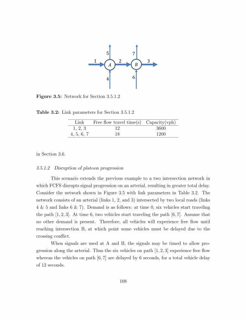
𝐴 𝐵 1 2 3
4
5
6
7
Figure 3.5: Network for Section 3.5.1.2
Table 3.2: Link parameters for Section 3.5.1.2
Link Free flow travel time(s) Capacity(vph)1, 2, 3 12 3600
4, 5, 6, 7 18 1200
in Section 3.6.
3.5.1.2 Disruption of platoon progression
This scenario extends the previous example to a two intersection network in
which FCFS disrupts signal progression on an arterial, resulting in greater total delay.
Consider the network shown in Figure 3.5 with link parameters in Table 3.2. The
network consists of an arterial (links 1, 2, and 3) intersected by two local roads (links
4 & 5 and links 6 & 7). Demand is as follows: at time 0, six vehicles start traveling
the path [1, 2, 3]. At time 6, two vehicles start traveling the path [6, 7]. Assume that
no other demand is present. Therefore, all vehicles will experience free flow until
reaching intersection B, at which point some vehicles must be delayed due to the
crossing conflict.
When signals are used at A and B, the signals may be timed to allow pro-
gression along the arterial. Thus the six vehicles on path [1, 2, 3] experience free flow
whereas the vehicles on path [6, 7] are delayed by 6 seconds, for a total vehicle delay
of 12 seconds.
108

For reservation controls, vehicles may request a reservation at the next inter-
section as soon as they can know their arrival time there. It is reasonable to assume
that vehicles will not request a reservation at an intersection until they enter an in-
coming link to that intersection, i.e. vehicles on link 1 traveling on path [1, 2, 3] will
not request a reservation at B. There are several reasons why vehicles might delay
their requests. First, unforeseen circumstances at intersection A, such as jaywalking
pedestrians, might delay vehicle movement across A. Second, vehicles using adaptive
routing to respond to congestion may not want to commit themselves to a turning
movement at B before getting closer to ascertain traffic conditions on outgoing links
of B. Even without this assumption, it is trivial to add additional demand on link
2 that prevents the vehicles on path [1, 2, 3] from requesting a reservation at B until
entering link 2. Under this condition, we find that reservations increase the total
delay.
When reservations are used, the vehicles on path [6, 7] can request a reservation
at B at time 6, when they enter link 6, because the link is at free flow. However, the
vehicles on path [1, 2, 3] cannot request a reservation until time 12, when they enter
link 2. With a time step of delay between reservations, any reservation policy that
does not account for future reservation requests — such as FCFS — will grant the
requests of vehicles on path [6, 7] because no conflicts are present at the time those
requests are made. Therefore, none of the six vehicles on path [1, 2, 3] can cross B at
time 24. These vehicles are delayed by 1 time step, resulting in a total vehicle delay
of 36 seconds.
Delaying acceptance of the reservation request until vehicles have moved closer
to the intersection may not completely solve the issue. In practice, more complex
reservation policies such as auctions must wait to collect all requests before making
a decision. However, the difference of 6 seconds in submitting reservation requests
in this example could easily be made greater by increasing the length of link 6.
Furthermore, vehicles may have to make late reservation requests due to traffic in
front, which reduces the margins the intersection manager has for delaying acceptance.
If the reservation policy were to anticipate future reservation requests, it could
avoid this situation. Traffic signals can “anticipate” these future requests by timing
109

cycles to allow for progression. Therefore any reservation policy that operates only on
existing reservations, such as FCFS or auctions, will grant vehicles on path [6, 7] the
reservation before vehicles on path [1, 2, 3] have even submitted their request. Another
way to handle this type of situation is to retroactively deny a reservation. Retracting
permission to enter an intersection adds complexity to the protocol: the vehicle with
a previous reservation must confirm that it will not execute it. Still, such a protocol
could be useful to warn vehicles of impending hazards such as pedestrians or collisions.
However, selfish vehicle programming might choose to ignore the retroactive denial
message if used to shift reservation priorities to game the system. Retroactive denial
would also introduce potential safety issues.
3.5.1.3 Arbitrarily large queues due to route choice
In the previous two examples, FCFS caused greater delays due to being less
optimized for the network structure than traffic signals. This example combines that
lack of optimization with selfish route choice to cause potentially infinite queuing. We
make the typical assumption of DTA that vehicles choose routes to minimize their
own travel time. This behavior results in a DUE: a route assignment in which no
vehicle can improve travel time by changing routes. This Wardrop (1952) equilibrium
has been shown to cause paradoxes in which network improvements increase travel
time for all vehicles (Braess, 1968; Daganzo, 1998). This scenario is perhaps the most
difficult to avoid because to do so requires some additional delay or toll on the local
road, even when there is no conflicting demand from the arterial.
We present a network based on Daganzo (1998)’s paradox in which replacing
a signal with a FCFS reservation-based control results in potentially infinite queuing.
Consider the four link network shown in Figure 3.6 with link parameters shown in
Table 3.3. Vehicles can take arterial link 2 or local road 3 to travel between B and
C. Assume that turning movements from links 2 and 3 to 4 conflict at C, i.e. 2400
vph may travel from 3 to 4, or 1200 vph from 2 to 4, or any convex combination.
Also assume that the diverge at B has sufficient capacity to support any turning
proportion split. Suppose that demand from A to D is 1800 vph. Since link 2 is
an arterial, suppose intersection C is controlled by a signal with considerable delays
110

for vehicle traveling from 3 to 4: the cycle is 60 seconds for movement from 2 to 4
then 10 seconds for movement from 3 to 4. Because of the average delay of nearly 30
seconds from the signal for vehicles traveling from 3 to 4, path [1, 3, 4] has an average
travel time of around 170 seconds. In contrast, path [1, 2, 4] has an average travel
time of around 140 seconds. Therefore, when all demand takes path [1, 2, 4], it is an
equilibrium, and the network is nearly at free flow.
Now suppose that the signal at C is replaced with a reservation control using
the FCFS policy. Because of the fairness attribute of FCFS, the expected delay for
vehicles moving from 3 to 4 is small: they can expect to alternate with vehicles
moving from 2 to 4. Because of this alternation, all demand on path [1, 2, 4] is not an
equilibrium, because path [1, 3, 4] has a travel time that is only slightly higher than
120 seconds — lower than the free flow time of path [1, 2, 4]. On the other hand, all
demand on path [1, 3, 4] is an equilibrium. Vehicles reaching B are presented with the
choice of taking link 2, with its free flow time of 80, or link 3, with its free flow time
of 60, and link 3 is always better. However, the 1200 vph capacity of link 3 creates a
queue on link 1. This queue can grow infinitely: if the demand of 1800 vph continues
for an infinite time, all demand on path [1, 3, 4] will still be the equilibrium, which
will result in the queue growing at the rate of 600 vph.
This scenario is similar to Daganzo (1998)’s paradox in that queuing before
the diverge results in vehicles choosing the least efficient route for the system. In
this example, once vehicles reach the diverge, they find free flow, or nearly free flow,
conditions on both alternative paths. Since link 3 has a much lower free flow time
than link 2, all vehicles choose the shorter link. When signals were in place this choice
was discouraged through an artificial delay placed on vehicles on link 3. With FCFS
reservations, the delay is removed in the interests of fairness.
From this example, we make the following conclusions: first, replacing a signal
with reservations can, in the worst case, result in arbitrarily long queues. Avoiding
this type of scenario is difficult because the queuing results from the choice of control
at C. In both scenarios, links 2, 3, and 4 are nearly at free flow. From the local
perspective of intersection C, both signals and reservations at C are managing demand
sufficiently. Identifying the congestion resulting from reservations at C requires a
111

A B C D 1 4
3
2
Figure 3.6: Network for Section 3.5.1.3
Table 3.3: Link parameters for Section 3.5.1.3
Link Free flow travel time(s) Capacity(vph)1 30 24002 80 24003 60 12004 30 2400
network perspective.
To stabilize this scenario, the control at C must impose some delay on move-
ment from 3 to 4. If vehicles are given preference by time spent waiting (such as
with FCFS) or even by some more system-related objectives such as maximum flow,
the unstable situation results. Furthermore, it is necessary to delay vehicles moving
from 3 to 4 even when no vehicles are waiting on link 2. This delay is contrary to
the goal of most reservation policies to maximize utilization of intersection capacity.
However, this delay could also be in the form of waiting time or in a toll placed
on movements from 3 to 4. Previous work on intersection auctions (Schepperle and
Bohm, 2008) provides the technology necessary for tolling specific turning movements
or microtolling every link.
3.5.2 Realistic networks
Having demonstrated the potential for signals to perform better than FCFS
reservations through theoretical examples, we now investigate such situations in re-
alistic networks. For these studies, we use CTM (Daganzo, 1994, 1995a) for dynamic
112

flow propagation with the conflict region algorithm (Section 3.4, which is consis-
tent with the constraints on general intersection models of Tampere et al. (2011) for
reservation-based control. Signals are modeled by calculating saturation flows for each
turning movement proportional to green times. We study three subnetworks of the
Austin regional network based on data from the Capital Area Metropolitan Planning
Organization. First, we present an arterial subnetwork and a highway subnetwork in
which signals or merges/diverges outperform reservations. Then, we compare FCFS
reservations to signals on the downtown Austin subnetwork, which includes both sig-
nals and merges/diverges. The positive results for this large network demonstrates
the potential benefits of reservations.
3.5.2.1 Arterial subnetwork
Lamar & 38th Street is the intersection between two arterials in Austin, shown
in Figure 3.7. It contains 5 signalized intersections and 21 links. The intersections
on Lamar (running southwest-northeast) do not have progression, but the two inter-
sections on 38th Street are timed for it.
Table 3.4 shows TSTT and travel time (TT) per vehicle at different demand
scenarios. (These results do not include the capacity and congested wave speed im-
provements discussed in Chapter 2.) Traffic signals consistently outperformed reser-
vations at all demand levels. Reservations appeared to scale somewhat worse with
demand as well. The worst performing links for reservations at 100% demand were
along the Lamar arterial. The southwestern region in particular had high travel
times with reservations. It is likely that FCFS reservations allowed vehicles entering
from local roads to delay vehicles traveling along the arterial, as discussed in Section
3.5.1.1. The intersections there are close together, and reduced intersection capacities
granted to the arterial by FCFS may have also resulted in queue spillback issues.
In addition, the progression on 38th Street was likely disrupted by the use of
reservation-based controls. In particular, in the DTA model vehicles do not request
a reservation from an intersection until after entering an incoming link. The gap
between the intersections of Lamar & 38th Street, and Medical Parkway and 38th
Street, is smaller than the length of the Medical Parkway link. This network topology
113

Figure 3.7: Lamar & 38th St.
admits scenarios such as the one in Section 3.5.1.2 in which vehicles on Medical
Parkway could place a reservation before vehicles on 38th Street.
Table 3.4: Results on Lamar & 38th St.
Demand Scenario TSTT TT per vehicle13841 Traffic signals 4060.8 hr 17.60 min(85%) FCFS reservations 4560.4 hr 19.77 min14655 Traffic signals 4937.0 hr 20.21 min(90%) FCFS reservations 5778.5 hr 23.66 min15469 Traffic signals 6160.6 hr 23.90 min(95%) FCFS reservations 7189.4 hr 27.89 min16284 Traffic signals 7159.5 hr 26.38 min
(100%) FCFS reservations 8809.1 hr 32.46 min
3.5.2.2 Freeway subnetwork
Most literature has considered replacing traffic signals with reservation-based
controls. However, the reservation protocol is general enough to be applied to any
intersection. Previous studies such as Hall and Tsao (1997) have considered using
114

autonomous vehicle technologies to improve highway on- and off-ramps. In addi-
tion, ramp metering to reduce freeway congestion has been well-studied in the lit-
erature (Papageorgiou and Kotsialos, 2000), and reservations with AVs would allow
complete enforcement of ramp metering. Therefore, it is likely that researchers will
consider using reservations to control freeway access. In this subsection we present an
example on replacing conventional unsignalized merge/diverge behavior with FCFS
reservation controls.
In DTA, we model merging via constraints on the receiving flow. With normal
merging behavior, the receiving flow is distributed among the upstream links by
capacity, with leftover receiving flow given to saturated approaches. With FCFS
reservations, receiving flow is distributed according to the vehicle order of request.
The I–35 corridor, shown in Figure 3.8, is a freeway subnetwork with 220 links.
(Many of the on- and off-ramps are difficult to see due to the length of the corridor).
All intersections are merges or diverges; none are traffic signals. Table 3.5 shows
travel times at different levels of demand. (These results do not include the capacity
and congested wave speed improvements discussed in Chapter 2.) Merges/diverges
consistently outperformed reservations at all demand scenarios. At low demand,
the differences were small, but as demand increased, FCFS scaled much worse than
merges/diverges. An analysis of link travel times found that most of the delays
occurred from vehicles entering the freeway. It is not clear why FCFS reservations
made it more difficult for vehicles to enter the freeway. Possibly the greater number
of lanes on the freeway allowed freeway vehicles to submit requests at a greater rate
(vehicles could not submit requests unless they were not blocked from entering the
intersection by vehicles in front). These delays could be indicative of an asymmetry
issue where the three lane freeway intersects with one lane on- and off-ramps. Based
on the long queues for vehicles entering the freeway, it appears that FCFS reservations
in this case skew too much towards freeway traffic and do not provide enough capacity
to the on-ramps.
115

Figure 3.8: I–35 corridor
116

Table 3.5: Results on I–35 corridor
Demand Scenario TSTT TT per vehicle64025 Merges/diverges 4089.7 hr 3.83 min(50%) FCFS reservations 6023.4 hr 5.64 min76830 Merges/diverges 5307.5 hr 4.14 min(60%) FCFS reservations 11912.9 hr 9.30 min89635 Merges/diverges 8049.8 hr 5.39 min(70%) FCFS reservations 23248.8 hr 15.56 min
3.6 Pressure-based policies for intersection control
The examples in Section 3.5 demonstrate that while FCFS is effective in some
situations, in other scenarios a better policy is needed before signals can be replaced
with reservations.
3.6.1 Link model
Describing backpressure requires a slightly different link representation than
discussed in Chapter 2. Recall that the traffic network is G = (N,A), where N is
the set of nodes, and A is the set of links. Let V be the set of demand. Each link
is divided into cells via CTM. Cells for link a ∈ A have length ufa∆t , where ufa is
the free flow speed of link a and ∆t is the simulation time step. Therefore, vehicles
can traverse at most one cell per time step. Let Γ−i and Γ+i be the incoming and
outgoing cells for i, respectively. Each cell is a FIFO queue of vehicles. Although the
hydrodynamic theory defines flow for continuous space and time, CTM approximates
the hydrodynamic theory by constraining flow between cells. As ∆t→ 0, the solution
to CTM approaches the solution to the hydrodynamic theory. CTM is commonly used
for large-scale or practical applications when solving the hydrodynamic theory exactly
is not tractable.
117

3.6.1.1 Cell flow dynamics
Our CTM formulation differs somewhat from that of Daganzo (1994, 1995a)
due to the need to track individual vehicles. Let ni(t) be the set of specific vehicles,
which will be necessary for defining which vehicles move at each time step. Let
Si(t) ⊆ ni(t) be the sending flow — the set of vehicles in cell i at time t that would
leave i if there were no downstream constraints. Let Ri(t) ∈ R+ be the receiving flow
of cell i at time t – the number of vehicles that would enter if connected to a source
of infinite demand. Let yvij(t) ∈ 0, 1 indicate whether vehicle v ∈ ni(t) moves from
cell i to cell j at time t. We extend yvij(t) from intersection movements to movements
between cells. If yvij(t) = 1, v moves from i to j at t. v will not move from i to j
unless j ∈ pv, which is important for intersection dynamics. Flow between i and j is
further constrained: v cannot leave i at t unless v ∈ Si(t). Also, the total flow into j
cannot exceed Rj(t). Formally,∑i∈Γ−j
∑v∈Si(t)
yvij(t) ≤ Rj(t) (3.25)
for all cells j. Also,
|Si(t)| ≤ Qi∆t (3.26)
where Qi is the capacity of cell i, and
Rj(t) = min
Qj∆t,
wjufj
(Nj − |nj(t)|)
(3.27)
where ufj is the free flow speed, wj is the congested wave speed, andNj is the maximum
occupancy of cell j.
Vehicle movement is also constrained by the FIFO behavior of cell queues.
Vehicles cannot exit if blocked by a vehicle in front. Finally, flow between links may be
constrained by intersection conflicts. Let yij(t) denote a vector of vehicle movements
for vehicles in Si(t). Let Yn(x(t)) denote the set of feasible vehicle movements across
node n ∈ N at t when cell occupancies are given by the vector n(t). Yn(n(t)) is
118

constrained by sending flow, receiving flow, path constraints, intersection conflicts,
and FIFO behavior.
Each yij(t) ∈ Yn(t) is an action that may be taken for moving flow. Let S(t)
be a vector of sending flows and Y(n(t)) be a vector of feasible movements across all
nodes at time t. A policy determines which vehicles are moved when the sending flow
is S(t).
The state of this system evolves according to conservation of flow:
nj(t+ 1) =nj(t) ∪ Vj(t) ∪
⋃i∈Γ−j
v ∈ Si(t) : yvij(t) = 1
/
⋃k∈Γ+
j
v ∈ Sj(t) : yvjk(t) = 1
(3.28)
where Vj(t) ⊆ V is the set of vehicles departing from cell j at time t.
Flow between two cells on a link (as opposed to flow across an intersection) is
clearly defined by the CTM (Daganzo, 1994, 1995a) in accordance with the kinematic
wave theory. Recall that vehicles on each cell are stored in a FIFO queue. CTM
defines the quantity of flow, and a corresponding number of vehicles from the FIFO
queue are moved. Therefore, for cells i, j on the same link, Yij(t) = 1. Flow between
two cells across an intersection may have more possibilities due to the intersection
conflicts.
3.6.2 Backpressure policy for reservations
We adapt the backpressure policy (Tassiulas and Ephremides, 1992) for the
traffic network. Due to DUE route choice (Section 3.5.1.3), we cannot prove that this
policy is a maximum throughput method. Nevertheless, results on a city network
show significant improvement over the FCFS policy.
119

3.6.2.1 Traffic network as constrained queuing system
A major difference between communications networks and traffic networks is
that in traffic networks, congestion creates regions of high-density, slower-moving
traffic. Communications networks are essentially point queues, and the size of the
queue does not affect link travel times. After a review of the communications network
of Tassiulas and Ephremides (1992), we show that our CTM traffic network is similar
to the constrained queueing systems that they studied. Each cell is a point queue,
and shockwaves in traffic flow are modeled through cell transition flows. This model
results in many queues — including multiple queues per link. Still, flows between
cells within a link are simple to handle because the feasible region is determined
exactly by cell transition flows. Of course, this relies on the CTM approximation to
the kinematic wave theory; the kinematic wave theory itself is continuous and can
be solved in continuous space (Yperman et al., 2005; Yperman, 2007). Nevertheless,
CTM is commonly used in large-scale DTA models, so using CTM to adapt the
backpressure policy is reasonable.
Although this cell model is equivalent to a communications network, there are
several issues that prevent proving that backpressure maximizes throughput. First,
queue sizes are bounded due to network geometry, and previous work on communi-
cations networks has required large queue sizes to ensure stability (Giaccone et al.,
2007; Le et al., 2012). While arbitrary queue sizes are possible in computer storage,
road lengths are not so arbitrary. Second, communications networks do not have
FIFO behavior. Due to different destinations, FIFO behavior at intersections limits
the feasible region of the control policy. For instance, a left-turning vehicle could
block a right-turning vehicle behind it, even though the right-turning vehicle could
otherwise move through the intersection. Finally, communications network policies
assume route choice is controlled by the system. However, in traffic networks, vehicles
typically choose routes individually, and DUE route choice can reduce efficiency.
Section 3.5.1.3 presented a counterexample to stabilizing the network via a
decentralized policy. Therefore, it is not possible to prove that any decentralized
pressure-based policy, including backpressure, is throughput optimal for a network
120

under UE route choice. It is true that previous work on applying backpressure (Zhang
et al., 2012a; Gregoire et al., 2014; Wongpiromsarn et al., 2014; Xiao et al., 2014)
were able to prove that backpressure was stable, if demand allowed it. However,
they assumed that turning proportions remained fixed, which is not true under DUE
behavior (Smith, 1979). The counterexample in Section 3.5.1.3 used DUE route choice
to create a situation in which the network can be stabilized, but will not be stabilized
under a decentralized pressure-based policy.
3.6.2.2 Maximum throughput heuristic
We adapt the backpressure policy of Tassiulas and Ephremides (1992) to the
CTM network. We cannot prove that backpressure maximizes throughput, but the in-
sights of backpressure control are used for this heuristic. Backpressure is an algorithm
executed each time step that determines intersection vehicle movements. Algorithm
4 gives a formal description of the backpressure policy. As with the algorithm of Tas-
siulas and Ephremides (1992), backpressure consists of three stages. Stage 1 selects
the weights on each vehicle based on cell queues. Stage 2 decides the combination of
vehicles to move given the vehicle weights. Note that the decision of which vehicles
to move can be separated by intersection: a system-wide controller is not necessary.
However, computing the vehicle weights in Stage 1 requires communication of queue
lengths between neighboring intersections.
For any node n, let Γ−n and Γ+n be the sets of incoming and outgoing cells,
respectively. Also let Γ−v,n and Γ+v,n be the incoming and outgoing cells for vehicle v
at n, respectively. To simplify the notation, let yvn(t) = yvΓ−v,n,Γ
+v,n
(t) denote whether
v moves through n at t.
The key insight is in the calculation of the pressure terms Dvn(t) for each
vehicle v at node n at time t. For communications networks, the pressure is simply
proportional to the queue size because queues are unbounded. A key requirement of
Tassiulas and Ephremides (1992)’s proof is that Dvn(t) can become arbitrarily large as
the queue grows. However, cell queues are bounded, so setting Dvn(t) = |nΓ−v,n
(t)| does
not provide sufficient pressure. Instead, we define a congestion region of connected
congested cells, and sum the occupancies of all cells in the congestion region.
121
Stage 1 This stage determines the vehicle weights Dvn(t) for each vehicle v. Since
the queue at cell j could be bounded, to achieve unbounded pressures we must con-
sider cells behind j. Even link queue lengths might be too small to provide sufficient
pressure (Giaccone et al., 2007; Le et al., 2012). Define Cj to be the set of congested
cells leading up to j. Cj is defined recursively as
Cj = j ∪i ∈ Γ−j′ : j′ ∈ Cj and |nj(t)| > Qj∆t
(3.29)
Equation (3.29) can be explained intuitively as follows: Cj is the set of congested cells
containing queued vehicles that might use cell j. We define cell j to be congested if
nj(t) > Qj∆t, which means that not all vehicles in j can exit in a single time step.
The queue at j is always considered, so j ∈ Cj. If j is not congested, Cj = j. If j is
congested, then Cj is the set of contiguous congested cells leading up to and including
j. If the network is sufficiently congested, then Cj will include one or more centroid
cells, which have unbounded queues. The pressure from the queues from the centroid
cell(s) will result in arbitrarily large pressure, which is one of the key features of the
backpressure policy.
Let pij(t) be the proportion of vehicles in cell i that have cell j in their path.
Clearly, pjj(t) = 1, and for any cell i preceding j on the same link, pij(t) = 1 also.
When queue spillback is present and i is on a different link than j, pij(t) < 1 is
possible.
Define the queue length for cell j at time t, Qj(t) to be
Qj(t) =∑i∈Cj
|ni(t)|pij(t) (3.30)
Qj is the number of vehicles in the congested region Cj waiting to use cell j. Now
define Dvn(t) as follows:
Dvn(t) =
(QΓ+
v,n(t)− QΓ−v,n
(t))
minQΓ+
v,n, QΓ−v,n
(3.31)
Dvn(t) is the product of the difference in queue lengths for cells Γ−v,n and Γ+
v,n and
122

the maximum flow rate between Γ−v,n and Γ+v,n. This product is taken directly from
Tassiulas and Ephremides (1992). Note that when Γ+v,n is a sink cell, QΓ+
v,n= ∞
and QΓ+v,n
(t) = 0 by definition. The difference is used because moving vehicles onto
a congested cell (if possible) is intuitively less efficient than moving vehicles onto
uncongested cells. Dvn(t) does not depend on properties of v besides the path of v.
The vehicle index is retained for vector notation; let D(t) be the vector of vehicle-
specific weights.
Stage 2 Find a vehicle movement vector y∗(t) satisfying the following:
y∗(t) ∈ arg maxy(t)∈Y(t)
D(t) · y(t) (3.32)
Note that equation (3.32) can be solved for individual intersections because the choice
of flows at a single intersection does not affect the feasible flows for other intersections
at the same time step.
Stage 3 If y∗vn (t) = 1, then vehicle v is moved from Γ−v,n to Γ+v,n at t. Otherwise, v
remains in Γ−v,n. This flow is feasible because y∗(t) ∈ Y(t).
Remarks Note that Stages 1 and 2 only need to be computed for incoming and
outgoing cells at nodes. For flow between two cells on the same link, there is only
one feasible solution as defined by the CTM transition flows (Daganzo, 1994, 1995a).
Stage 2 requires the solution of an integer program, which is NP-hard. For
reservation-based intersection control, vehicles may be allowed to move individually,
which could result in a large feasible region. |Yn(t)| is O(2|Sn(t)|). For tractability,
we use the polynomial-time greedy heuristic of Section 3.4.2 to find a decent solution.
In calculating the efficiency, we set z(t) = D(t) in equation (3.24).
3.6.2.3 A note on practical implementation
One potential concern is how to implement the backpressure policy in practice.
CTM is itself an approximation to the hydrodynamic theory, and defining the policy
123

in terms of cell queues may not seem completely realistic. However, as ∆t → 0,
the predictions of CTM approach those of the hydrodynamic theory. Therefore, the
calculation of the intersection queue length from the queues in contiguous congested
cells becomes the length of the queues on intersection approaches. The size of these
queues may be determined through loop detectors.
A second issue with implementation is calculating the total length of queues
across queue spillback. In the backpressure, we assumed that we know vehicle routes,
and whether they will use any given cell. In practice, vehicle routes may not be
known, even for autonomous vehicles. Queues specific to a link could be estimated
by turning fractions when queue spillback is present. However, these turning fractions
may change over time due to DUE route choice.
Our traffic network model also assumes that centroid queues will grow ar-
bitrarily large if demand is sufficiently high. Realistically, travelers will probably
choose to depart later if queues are backed up to their origin. However, when de-
mand is modeled as elastic, boundedness of queue length is not an effective measure
of stability.
3.6.3 P0 policy for reservations
The backpressure policy is from a model where routing is determined by the
system (Tassiulas and Ephremides, 1992) and the counterexample to stability (Sec-
tion 3.5.1.3) shows that DUE route choice could prevent stability. In the worst case,
policies relying on local information could result in unbounded queues despite a sta-
bilizable demand. Therefore, we also adapt the P0 policy (Smith, 1980, 1981) to
reservations for comparison. P0 is an algorithm run at each time step, described
formally in Algorithm 5. P0 was designed to maximize network capacity under UE
route choice. However, proving that P0 maximizes capacity in the simulation-based
CTM is difficult because link travel times are not continuous with respect to inflow or
demand. P0 also uses a congestion-increased pressure term, but the pressure is based
on link travel times rather than queue lengths.
P0 was designed for a model using link performance functions for delay. Specif-
124

Algorithm 4 Backpressure policy
1: for all a ∈ A do2: Let j be the end cell of a3: Set Cj = Find congested region(j)4: for all v ∈ nj(t) do5: Qj(t) :=
∑i∈Cj
|ni(t)|pij(t)
6: end for7: end for8: for all n ∈N do9: for all v ∈ Sn(t) do
10: f(v) :=(QΓ+
v,n(t)− QΓ−v,n
(t))
minQΓ+
v,n, QΓ−v,n
11: end for12: Conflict region algorithm(n)13: end for14:
15: procedure Find congested region(j)16: Cj := j17: if |nj(t)| > Qj(t) then18: for all i ∈ Γ−j do19: Cj := Cj∪ Find congested region(i)20: end for21: end if22: return Cj23: end procedure
125

ically, P0 assumes that the travel time τa for link a ∈ A is of the form
τa = τ fa + fa
(ωa + µaQa
)(3.33)
where τ fa is the free flow travel time, fa(·) is the delay function, ωa is the demand for
the link, Qa is saturation flow, and µa is the proportion of red time. For phase k at
node n ∈ N let Akn ⊆ A be the set of links given green time. For a link travel time
of this form, the resulting pressure ρkn for phase k is then
ρkn =∑a∈Ak
n
Qafa
(ωa + µaQa
)(3.34)
Applying equation (3.34) to DTA requires evaluating the function fa(·), which is de-
termined through simulation in DTA. However, previous travel times are observable.
Let τa(t) be the expected travel time for link a at time t, based on estimates from
vehicles that traversed a. Then we create an estimate of fa(·) at t, fa(t), by taking
fa(t) = τa(t)− τ fa (3.35)
We also replace saturation flow Qa with capacity Qa. In practice, these may not be
equivalent since many static models assume that link flows can exceed the saturation
flow at the cost of high delay. However, capacity is the flow constraint parameter for
DTA.
We adapt P0 to reservation-based intersection control, meaning that pressure
is specified for specific vehicles rather than phases. Since the pressure is based on the
link travel time, let a−1v,n ∈ A be the incoming link for vehicle v at node n. (The link
a−1v,n differs from the incoming cell because the pressure for P0 is based on the link
travel time, not the cell travel time). We use the following pressure Pvn(t) for vehicle
v at node n at time t using the P0 policy:
Pvn(t) = Qa−1v,n
(¯τa−1v,n
(t)− τ fa−1v,n
)(3.36)
Pvn (t) favors links with high capacity and/or with a high delay (travel time beyond
126

the free flow time). Delay should greatly increase as the queue length increases.
Define the vector of pressures to be P(t) for all waiting vehicles. The objective
is then to find
y∗(t) ∈ arg maxy(t)∈Y(t)
P(t) · y(t) (3.37)
As with the backpressure policy, equation (3.37) can be determined locally for in-
dividual intersections. We also approximately solve equation 3.37 using the greedy
heuristic of Section 3.4.2. To calculate the efficiencies, we set z(t) = P(t) in equation
(3.24).
Algorithm 5 P0 policy
1: for all n ∈N do2: for all v ∈ Sn(t) do
3: f(v) := Qa−1v,n
(¯τa−1v,n
(t)− τ fa−1v,n
)4: end for5: Conflict region algorithm(n)6: end for
3.7 Experimental results
We compared four types of intersection controls — traffic signals and reserva-
tions with FCFS, backpressure, and P0 — on the downtown Austin network, shown in
Figure 2.15. The network has 171 zones, 546 intersections, and 1247 links. Data was
from the Capital Area Metropolitan Planning Organization. The DNL used CTM
with a 6s time step, and the conflict region model for reservation-based intersection
control. Traffic signals were modeled by simulating phases and changing the capac-
ity of turning movements proportional to green time at each time step. Flow was
discretized and individual vehicles were tracked. We used the method of successive
averages (Levin et al., 2015b) to solve DTA to a 1% gap for all scenarios. To demon-
strate robustness, we considered demand levels from 70% to 100% at 10% increments.
Table 3.6 compares the travel times for all four intersection control policies at
different demand levels. Reservations using all policies (including FCFS) consistently
127

had much lower TSTT than traffic signals. Although Section 3.5 discussed several
situations in which FCFS reservations would increase delay compared with signals,
there are also scenarios (such as symmetric intersections) in which FCFS is likely to
reduce delay (Fajardo et al., 2011; Li et al., 2013). Both backpressure and P0 made
significant improvements over FCFS as well. This result is not surprising because
FCFS does not prioritize links with higher demand, which could cause queues to
build up and spillback on such links. Backpressure also consistently performed slightly
better than P0. This result is probably because backpressure is more responsive to
current traffic conditions than P0. P0 was developed for a model with link performance
functions, in which travel times could be easily calculated. However, in simulation-
based DTA, travel times are determined by simulation. Therefore, high travel times
were only observed after vehicles had exited the link, which delayed the effect of
queuing on the P0 prioritization. In contrast, backpressure prioritized based on queue
lengths at the current time. Therefore, backpressure responded faster and more
dynamically to congestion and queueing.
3.8 Conclusions
This chapter developed and optimized a simplification of tile-based reserva-
tions (Dresner and Stone, 2004) for autonomous vehicles. We first formulated an IP
for the conflict point transformation of tile-based reservations (Zhu and Ukkusuri,
2015). After transforming the IP for use in SBDTA, the spacing constraints were
found to naturally reduce to capacity limitations on each conflict point. For com-
putational tractability on large networks, we aggregated conflict points into conflict
regions, resulting in a model similar to that of Levin and Boyles (2015b) formulated
as an IP. This IP admits arbitrary objective functions and can therefore be used
to optimize the order that vehicles cross the intersection for a more general class of
policies. Since IPs in general are NP-hard, we derived theoretical results about the
conflict region algorithm (Levin and Boyles, 2015b). It solves the IP for the FCFS ob-
jective, and admits a polynomial-time greedy heuristic based on the MCKS problem
for general objective functions.
128

Table 3.6: Intersection control results on downtown Austin network
Demand Intersection policy TSTT (hr) Avg. TT per vehicle (min)43965 Traffic signals 8552.2 11.67(70%) FCFS 4276.6 5.84
Backpressure 3974.0 5.42P0 4003.1 5.46
50290 Traffic signals 10771.5 12.9(80%) FCFS 5550.4 6.62
Backpressure 4819.7 5.74P0 4897.6 5.84
56592 Traffic signals 13776.0 14.61(90%) FCFS 7116.0 7.55
Backpressure 6016.1 6.38P0 6285.6 6.66
62847 Traffic signals 16971.6 16.20(100%) FCFS 9334.2 8.91
Backpressure 7815.5 7.46P0 8397.1 8.01
Results for signals and FCFS differ slightly from other reported numbers for the same network be-
cause the discrete vehicle trips were recreated from a dynamic trip table, resulting in some stochas-
ticity in the demand.
129

To motivate optimization of reservations, this chapter presented a variety of
scenarios in which traffic signals and merges/diverges outperformed reservations. We
studied three theoretical situations using the different attributes of FCFS reservations
to increase delays. One example showed that decentralized reservation policies could
create a Daganzo (1998) paradox situation due to DUE route choice. We also pre-
sented two realistic networks from Capital Area Metropolitan Planning Organization
data in which traffic signals or merges/diverges outperformed reservations.
Finally, we adapted the backpressure (Tassiulas and Ephremides, 1992) and
P0 (Smith, 1980, 1981) policies for reservation-based intersection control in dynamic
traffic assignment. Neither can be proven to stabilize the network because they are
both decentralized policies. Nevertheless, results on the downtown Austin network
showed that backpressure and P0 performed significantly better than the first-come-
first-served policy, which has been used in most previous work on reservations. There-
fore, although backpressure and P0 are not throughput-optimal, they provide a better
alternative to existing policies.
130

4 Applications
4.1 Introduction
Most previous studies of AVs have relied on microsimulators to capture AV
behavior differences, but micro-simulation is not tractable for large network analyses.
Carlino et al. (2012) simplified the reservation controls to simulate a city network,
but the capacity of the reservation mechanism was reduced and they did not include
route choice. Ideally, analyses of large networks would be based on DTA, which
includes the effects of selfish route choice. Chapter 2 developed a multiclass version
of the CTM (Daganzo, 1994, 1995a) with a corresponding car-following model that
predicts increases in capacity and backwards wave speed as reaction-time decreases,
and Chapter 3 developed a conflict region simplification of the reservation protocol
that is tractable for DTA. The purpose of this chapter is to use the resulting DNL
and DTA models to study how AVs affect congestion and travel demand on larger
networks.
4.1.1 Improved road efficiency
First, we study how increasing market penetration of AVs affects freeway,
arterial, and downtown network traffic. Since previous studies have relied on mi-
crosimulation, network size was limited by the computational intensity. Therefore,
it is both novel and relevant to practitioners to study how AVs might affect traffic
before including changes to travel demand.
131

4.1.2 Empty repositioning trips
With regards to travel demand, Levin and Boyles (2015a) created a four-step
model including empty repositioning to the origin as a modal alternative to parking
for home-to-work trips. Results indicated that the significant additional vehicular
demand offset increased road efficiency, resulting in a net increase in congestion.
They found that empty repositioning increased the number of travelers choosing to
drive, and combined with the return trips from repositioning, resulted in nearly twice
as many total vehicular trips.
For policymakers, the results of Levin and Boyles (2015a) raise the question of
why to permit repositioning trips at all. However, their model was not very realistic
as it relied on a STA model to predict congestion. Their model could be improved in
several ways:
1. Because the model is based on STA, different departure times were not included.
By definition, empty repositioning from home-to-work trips should depart later
(after the traveler arrived at work). The later departure times might result in
an extended morning peak as opposed to a more concentrated one with greater
congestion (Levin, 2015).
2. The model did not include the potential benefits from reservation-based in-
tersection control. Having more AVs on the road could improve intersection
efficency, which is a major bottleneck in downtown networks.
3. The link capacity model — how AVs improve link capacity — was preliminary
and could be improved by the work in Chapter 2
4.1.3 Shared autonomous vehicles
An even more radical change in travel behavior is the use of SAVs instead of
personal vehicles. SAVs are a fleet of autonomous SAVs that provide low-cost service
to travelers, possibly replacing the need for personal vehicles. Previous studies (Fag-
nant and Kockelman, 2014; Burns et al., 2013) assuming that all travelers used SAVs
found that each SAV could service multiple travelers, reducing the number of vehicles
132

needed in the SAV fleet. Although 100% SAV use is unlikely to occur in the near
future, previous results suggest great potential benefits when 100% SAVs becomes
viable. Strategies such as preemptive relocation of SAVs for expected demand (Fag-
nant and Kockelman, 2014) or dynamic ride-sharing (Fagnant and Kockelman, 2016)
are additional options for improving service.
However, a major limitation of previous studies is that many relied on custom
software packages with unspecified or unrealistic congestion models (Burns et al.,
2013; Fagnant and Kockelman, 2014, 2016; Spieser et al., 2014) and/or grid net-
works (Fagnant and Kockelman, 2014, 2016). Although these were important studies
for technology demonstration purposes, for accurate comparisons with personal ve-
hicle scenarios a common traffic flow model is necessary. This chapter develops a
framework compatible with existing traffic simulation models. This framework allows
practitioners to integrate SAVs into their current traffic models to evaluate whether
to fund public fleets of SAVs.
This framework admits a DNL model of SAVs using CTM (Daganzo, 1994,
1995a). We compare SAVs using heuristics for vehicle routing and dynamic ride-
sharing based on previous work (Fagnant and Kockelman, 2014, 2016) against per-
sonal vehicle scenarios. Heuristics are used because the vehicle-routing problem is
NP-hard (Toth and Vigo, 2001). The framework allows us to study SAV behaviors
using the DNL model developed in Chapters 3 and 2.
4.1.4 Contributions
The contributions of this chapter are as follows:
1. We analyze the effects of reservation controls and increased capacity from AV
technologies on freeway and arterial networks using DTA. We studied a variety
of congested subnetworks and drew conclusions that can be generalized to other
locations. For most scenarios, reservations improved over traffic signals for
arterial networks (and the freeway network that used signals to control access),
but were not effective at replacing merges/diverges. Reduced reaction times,
resulting in reduced following headways and increased capacity, improved travel
133

times for all scenarios. We also studied the downtown Austin network, which
includes many route choice options, and found that the combination of these
AV technologies could reduce travel times by 78%.
2. We present a four-step model with departure time choice, using DTA, to study
how AVs affect travel demand. Link capacity increases and reservation-based
intersection control are included in DTA, and empty repositioning to the ori-
gin (as opposed to parking) is modeled as a mode choice using a nested logit
model. We use this model to study how empty repositioning trips affect traffic
on the downtown Austin city network during the morning peak. From a policy
perspective, we demonstrate two important conclusions: empty repositioning
trips can improve traffic by encouraging travelers to adopt AVs. Also, in the
scenario that all travelers have AVs, empty repositioning results in higher ve-
hicular demand and therefore greater congestion. Taken together, these results
suggest that allowing empty repositioning trips is worth consideration despite
the increase in vehicle trips.
4.1.5 Organization
The remainder of this chapter is organized as follows. Section 4.2 discusses
literature on planning models and SAVs. Section 4.3 studies how AVs affect arterial,
freeway, and downtown networks. The effects of repositioning trips are modeled
in Section 4.4. In Section 4.5, we develop a framework for implementing SAVs in
general traffic simulators, and perform a case study using our DNL model. Section
4.6 presents our conclusions.
4.2 Literature review
First, we review the literature on planning models in Section 4.2.1, which is
relevant to our study on empty repositioning trips. Then, we review work on SAVs
in Section 4.2.2 in anticipation of our SAV model.
134

4.2.1 Planning and forecasting
Forecasting in practice has been based on the four-step planning model (Mc-
Nally, 2008) for decades. The four-step model traditionally uses STA, although DTA
admits more accurate predictions of flow propagation and more detailed models of
AV intersections. 90% of practitioners would like to incorporate DTA into their plan-
ning analyses (Chiu et al., 2011), and previous studies (Tung et al., 2010; Pool, 2012;
Duthie et al., 2013) have replaced STA with DTA by using average travel times for
feedback and an exogenous departure time profile to disaggregate demand by assign-
ment intervals. However, modeling departure time choice is critical for this chapter
because the distribution of vehicular trips — both from travelers and for empty repo-
sitioning — determines the level of congestion. Vovsha et al. (2012) considered a
time-dependent mode choice model, but still use a fixed time distribution profile,
which is a major issue with DTA planning models (Peeta and Ziliaskopoulos, 2001).
Most time profile literature focuses on simultaneous route and departure time choice
(SRDTC) (Li et al., 1999; Ziliaskopoulos and Rao, 1999; Friesz et al., 2001), which
typically exclude the trip distribution and mode choice of four-step models and are
focused on short-term behavior. For instance, Szeto and Lo (2004) and Han et al.
(2011) studied SRDTC models with cell-based DTA and elastic demand. However,
trip distribution and mode choice also predict transit ridership, which may decline
significantly with AVs (Levin and Boyles, 2015a). Levin et al. (2016a) proposed a
time-varying trip distribution based on the arrival time penalty function (Vickrey,
1969) which addresses the DTA integration issue by adding a time index to the rest
of the four-step model.
Activity-based modeling (ABM) (Bhat and Koppelman, 1999) is a relatively
recent alternative to the traditional four-step model that may be more effective at
modeling empty repositioning trips. In addition to avoiding parking costs, empty
repositioning can make an AV available to other household members, and the benefits
of household car sharing are better modeled through ABM. However, integrating
ABM with DTA requires more study, particularly in the feedback of DTA travel times
to ABM. Furthermore, the four-step model is well established among metropolitan
135

planning organizations for long-range predictions. Therefore, this chapter uses the
four-step model.
4.2.2 Shared autonomous vehicles
Multiple studies have investigated the possibility of using a fleet of SAVs to
reduce reliance on personal vehicles and improve mobility and safety (Fagnant and
Kockelman, 2015). Fagnant and Kockelman (2014) estimated that one SAV could
provide service to around eleven travelers on a grid network approximation of Austin,
Texas with most travelers waiting at most 5 minutes for pick-up, although vehicle
travel time increased. Fagnant and Kockelman (2016) incorporated dynamic ride-
sharing, and found that it could offset the additional vehicle travel time. However,
only 10% of personal trips of Austin were included. Further studies on different cities
have supported indications that a smaller fleet of SAVs could provide service to all
travelers. Burns et al. (2013) studied a centrally dispatched SAV system in three
different urban and suburban environments. Their findings indicated that a much
smaller fleet of SAVs could provide service to all residents with acceptable waiting
times. Also, a slightly reduced fleet of taxicabs could improve on wait times and
vehicle utilization in Manhattan, New York. Spieser et al. (2014) found that a SAV
fleet one-third the size of the personal vehicle fleet was sufficient for providing service
to Singapore travelers.
Although the results of previous studies are encouraging, this chapter ad-
dresses some traffic modeling limitations of previous studies. All of them used cus-
tom simulation-based models, with many relying on grid-based networks. Many of the
traffic congestion models were unrealistic; Fagnant et al. (2015) used MATSim, but
many other studies did not specify the model or used fixed travel times. Section 4.5.3
demonstrates that SAVs could significantly increase congestion. Accurate congestion
modeling is necessary to evaluate whether replacing personal vehicles with SAVs im-
proves traffic. Furthermore, custom simulations would be difficult for practitioners
to integrate into their existing traffic models. To address these limitations, this chap-
ter presents an event-based framework that may be implemented on top of many
simulation-based traffic models. We demonstrate this framework by implementing it
136

in a DTA simulator and comparing SAV results with those from DTA.
4.3 Effects of autonomous vehicles on network traffic
This section presents analyses on arterial (Section 4.3.1), freeway (Section
4.3.2), and downtown (Section 4.3.3) networks using the multiclass CTM of Chap-
ter 2 to propagate flow in DTA. The key features of these results are the multiclass
comparison of human and autonomous vehicles, and the analysis of how reservations
compare to signals. The fundamental diagram changes with space and time in re-
sponse to the proportion of AVs in each cell. When combined with discrete vehicles,
the fundamental diagram varies significantly between cells and time steps despite an
overall fixed proportion of AVs. Reservation-based intersection control also exhibited
unusual characteristics. Contrary to the results of Fajardo et al. (2011) and Li et al.
(2013), reservations performed worse than signals in many scenarios due to subopti-
mal vehicle priority. In addition, Braess (1968) and Daganzo (1998) showed that the
increased link capacity due to AVs does not necessarily result in improved network
performance.
The arterial and freeway networks do not have multiple available routes, so
all improvements are due to AV technologies. However, the downtown networks in-
clude many alternate routes, which admits paradoxes in which capacity improvements
increase congestion due to selfish route choice (Braess, 1968; Daganzo, 1998). The
reaction times of AVs was set to 0.5 seconds, which significantly increases capacity
(Figure 2.2). Smaller reaction times might be more realistic of automation, but could
result in backwards wave speed exceeding free flow speed, causing technical issues
with the cell transmission model. For all experiments, we recorded the TSTT as well
as the average travel time per vehicle.
4.3.1 Arterial networks
We first present results on two arterial networks, shown in Figure 4.1. The first
arterial network, Lamar & 38th Street, contains the intersection between the Lamar &
38th Street arterials, as well as 5 other local road intersections. This network contains
137

Lamar & 38th Street Congress Avenue
Figure 4.1: Arterial networks
31 links, 17 nodes and 5 signals with a total demand of 16,284 vehicles over a 4 hour
time period. We also studied Congress Avenue in Austin, with a total of 25 signals
in the network, 216 links and 122 nodes with a total demand of 64,667 vehicles in a 4
hour period. These arterial networks used fixed-time signals for controlling flow along
the entire corridor. These networks were chosen for this experiment because they are
among the 100 most congested networks in Texas, which is useful for studying how
AVs affect congestion. By changing the demand on these networks, our analyses can
be generalized to less congested networks.
Travel time results are given in Tables 4.1 and 4.2. In the Lamar & 38th
Street network, the reservation protocol significantly decreased travel times for a 50%
demand simulation as compared to traffic signals at 50% demand; however, once
the demand was increased to 75%, reservations began increase travel times relative to
signals. This result is most likely due to the close proximity of the local road intersec-
tions. On local road-arterial intersections, the fairness attribute of FCFS reservations,
138

Table 4.1: Lamar & 38th Street results
Intersections Demand Proportion of TSTT Travel time perAVs (hr) vehicle (min)
Signals 50% 0% 421.6 3.11Signals 50% 100% 237.2 1.75
Reservations 50% 100% 157.8 1.16Signals 75% 0% 2566.7 12.61Signals 75% 100% 372.7 1.83
Reservations 75% 100% 2212.5 10.78Signals 85% 0% 3890.2 16.86Signals 85% 25% 2097.2 9.09Signals 85% 50% 504.8 2.19Signals 85% 75% 477.8 2.07Signals 85% 100% 476.8 2.07
Reservations 85% 100% 4472.8 19.39Signals 100% 0% 7043.1 25.95Signals 100% 100% 526.6 1.94
Reservations 100% 100% 8678.7 31.98
could give greater capacity to the local road than would traffic signals. Because these
intersections are so close together, reservations likely induced queue spillback on the
arterial. The longer travel times might also be influenced to reservations removing
signal progression on 38th Street. In high congestion, FCFS reservations tended to
be less optimized than signals for the local road-arterial intersections. On the other
hand, in low demand, intersection saturation was sufficiently low for reservations to
reduce delays.
The Lamar & 38th Street network responded well to an increase in the propor-
tion of AVs with dramatic decreases in travel times, due to the AV reaction times. At
85% demand and at 25% AVs, the total travel time was reduced by 50%, and when all
vehicles were AVs, the total travel time was reduced by 87%. As demand increased,
the improvements from reduced reaction times also increased. At 50% demand, re-
duced reaction times decreased travel time by 44%, whereas at 100% demand, reduced
139

Table 4.2: Congress Avenue results
Intersections Demand Proportion of TSTT Travel time perAVs (hr) vehicle (min)
Signals 50% 0% 1366.1 2.54Signals 50% 100% 1220 2.26
Reservations 50% 100% 821.5 1.52Signals 75% 0% 4306.1 5.33Signals 75% 100% 1957.1 2.42
Reservations 75% 100% 1545.1 1.91Signals 85% 0% 8976.8 9.8Signals 85% 25% 3661.4 4Signals 85% 50% 3303.3 3.61Signals 85% 75% 2936.2 3.21Signals 85% 100% 2956 3.23
Reservations 85% 100% 2934 3.2Signals 100% 0% 21484.4 19.93Signals 100% 100% 4038.2 3.75
Reservations 100% 100% 8673.6 8.05
140

reaction times decreased travel time by 93%. The effect of greater capacity improved
as demand increased because as demand increased, the network became more limited
by intersection capacity. At low congestion (50% demand), signal delays dominated
travel times because reservations made significant improvements. At higher conges-
tion, intersection capacity was the major limitation, and therefore reduced reaction
times were of greater benefit.
Congress Avenue responded well to the introduction of reservations, showing
decreases in travel times at all demand scenarios. These improvements are due to the
large amount of streets intersecting Congress Avenue, each with a signal not timed
for progression. The switch to reservations therefore reduced the intersection delay.
However, the switch to reservations could result in greater demand on this arterial.
We include the effects of route choice in the downtown Austin network (Section 4.3.3).
AVs also improved travel times and congestion due to reduced reaction times.
At 85% demand, even a 25% proportion of AVs on roads decreased travel times
by almost 60%. This benefit increased to almost 70% when all vehicles were AVs.
As with Lamar & 38th Street, as demand increased, the improvements from AV
reaction times also increased. For example, at 50% demand, 100% AVs decreased
travel time by about 10%, but at 100% demand, using all AVs reduced the travel
time by nearly 82%. The reduced reaction times did not improve as much as the
reservation protocol, except for the 100% demand scenario. This experiment indicates
that at lower demands, travel time was primarily increased by signal delay, but was
still improved by AV reaction times.
Overall, these results consistently show significant improvements from reduced
reaction times of AVs at all demand scenarios. As shown in Figure 2.2, reducing the
reaction time to 0.5 seconds nearly doubles road and intersection capacity. However,
the effects of reservations were mixed. At low congestion, traffic signal delays had a
greater effect on travel time, and in these scenarios reservations improved. Reserva-
tions also improved when signals were not timed for progression (although this change
in protocol may be detrimental to the overall network). However, as seen on Lamar &
38th Street, at high demand reservations performed worse than signals, particularly
around local road-arterial intersections.
141

Interstate 35
US-290
Mopac
Figure 4.2: Freeway networks
4.3.2 Freeway networks
Next, we studied three freeway networks, shown in Figure 4.2. The first free-
way network is the I–35 corridor in the Austin region which includes 220 links and
220 nodes with a total demand of 128,051 vehicles within a 4 hour span. (Due to the
length, the on- and off-ramps are difficult to see in the figure.) All intersections are
off-ramps or on-ramps. The I–35 network is by far the most congested of the freeway
networks and one of the most congested freeways in all of Texas, especially in the
Austin region. We also studied the US–290 network in the Austin region with 97
links, 62 nodes, 5 signals and a total demand of 11,098 vehicles within 4 hours. Fi-
nally, we studied the Mopac Expressway in the Austin region with 45 links, 36 nodes,
and 4 signals with a total demand of 27,787 vehicles within 4 hours. This network
includes a mix of merging and diverging ramps and signals which allows some inter-
esting analyses. This network was chosen due to the large number of signals around
the freeway. All freeway networks are also among the 100 most congested roads in
Texas.
Results for the freeway networks are presented in Tables 4.3, 4.4, and 4.5.
142

Table 4.3: I–35 results
Intersections Demand Proportion of TSTT Travel time perAVs (hr) vehicle (min)
Signals 50% 0% 3998.9 3.75Signals 50% 100% 3893.3 3.65
Reservations 50% 100% 3975.2 3.73Signals 75% 0% 10087 6.3Signals 75% 100% 5934.2 3.71
Reservations 75% 100% 9861.1 6.16Signals 85% 0% 16127.7 8.89Signals 85% 25% 16023.5 8.83Signals 85% 50% 15944.3 8.79Signals 85% 75% 14545.3 8.02Signals 85% 100% 14101.6 7.77
Reservations 85% 100% 16084.7 8.87Signals 100% 0% 31611.7 14.81Signals 100% 100% 9063.3 4.25
Reservations 100% 100% 30211.3 14.16
143

Table 4.4: US–290 results
Intersections Demand Proportion of TSTT Travel time perAVs (hr) vehicle (min)
Traditional 50% 0% 557.8 6.03Traditional 50% 100% 547.5 5.92
Reservations 50% 100% 505.4 5.47Traditional 75% 0% 845.7 6.1Traditional 75% 100% 827.7 5.97
Reservations 75% 100% 759.8 5.48Traditional 85% 0% 997.6 6.35Traditional 85% 25% 952 6.06Traditional 85% 50% 945.3 6.01Traditional 85% 75% 942.5 6Traditional 85% 100% 939.8 5.98
Reservations 85% 100% 860.6 5.47Traditional 100% 0% 1518.5 8.21Traditional 100% 100% 1108.8 5.99
Reservations 100% 100% 1014.1 5.48
Although there were some observed improvements in travel times for US–290 using
reservations, the improvements were modest. For I–35 and Mopac, reservations made
travel times worse for all demand scenarios. Most of the access on US–290 is controlled
by signals, which explains the improvements observed when reservations were used
there. Reservations seem to have worked more effectively with arterial networks,
probably because on- and off-ramps do not have signal delays. Therefore the potential
for improvement from reservations is smaller.
Overall, greater capacity from AVs reduced reaction times improved travel
times in all freeway networks tested, with better improvements at higher demands.
Reduced reaction times improved travel times by almost 72% at 100% demand on
I–35. On US–290 and I–35, as with the arterial networks, the improvement from AV
reaction times increased as demand increased. These benefits are because freeways
are primarily capacity restricted. On Mopac, reaction times had a smaller impact,
144

Table 4.5: Mopac results
Intersections Demand Proportion of TSTT Travel time perAVs (hr) vehicle (min)
Traditional 50% 0% 373.9 1.61Traditional 50% 100% 363.6 1.57
Reservations 50% 100% 409.9 1.77Traditional 75% 0% 576.6 1.66Traditional 75% 100% 554.9 1.6
Reservations 75% 100% 616.1 1.77Traditional 85% 0% 667.9 1.7Traditional 85% 25% 651.1 1.65Traditional 85% 50% 647.8 1.65Traditional 85% 75% 645.2 1.64Traditional 85% 100% 644.1 1.64
Reservations 85% 100% 698.7 1.77Traditional 100% 0% 1288.3 2.78Traditional 100% 100% 752.1 1.62
Reservations 100% 100% 825.4 1.78
but the network overall appeared to be less congested.
We also analyzed several groups of links and nodes in depth. Links and nodes
were chosen to study how reservations affected travel times at critical intersections,
such as high demand on- or off-ramps. For these specific links, we compared average
link travel times between 120 and 135 minutes into the simulation, at the peak of the
demand. We compared human vehicles, AVs with signals, and AVs with reservations
at 85% demand, which resulted in moderate congestion. In the I–35 network, very
few changes in travel times for the critical groups of links were observed from the
different intersection controls.
The differences seemed to be greater in the US–290 corridor with more over-
all improvements in critical groupings of links near intersections. Interestingly, the
largest improvements in travel times going from traffic signals to reservations occurred
at queues for right turns onto the freeway. A possible explanation for this result is
145

that making a right turn conflicts with less traffic than going straight or making a left
turn. Although signals often combine right-turn and straight movements, reservations
could combine turning movements in more flexible ways. Although larger improve-
ments in travel times occurred at the observed right turns, improvements at left turns
were also observed. Because US–290 has signals intermittently spaced throughout its
span, vehicles are frequently stopping for signal delays. Using the reservations sys-
tem, the flow of traffic is stopped less frequently, reducing congestion. The use of AVs
rather than HVs also helped travel times but by less than reservations. In most cases,
using reservations instead of signals doubled the improvements resulting from using
AVs. Reservations appear to have a positive effect on traffic flow and congestion in
networks (freeway and arterial) that use signals to control intersections.
4.3.3 Downtown network
Downtown Austin, shown in Figure 2.15, contains the downtown grid, several
major arterials, and part of I–35 on the east side. Overall, it has 171 zones, 546
intersections, 1247 links and 62836 trips. Network and demand data was from the
Capital Area Metropolitan Organization for the AM peak.
Downtown Austin is an useful test network because flow in the downtown grid
is primarily restricted by intersections. Unlike the previous two subnetworks, down-
town Austin contains different route options for vehicles. These route choices admit
scenarios like the Braess (1968) and Daganzo (1998) paradoxes, and the paradox of
Section 3.5.1.3. We considered two scenarios: first, using traditional intersections
(traffic signals and merges/diverges), and second, replacing all intersection controls
with FCFS reservations. To compare traditional intersections and reservations, we
first solved DTA using the method of successive averages. Both scenarios were solved
to a 2% gap.
Table 4.6 shows the results from solving DTA on downtown Austin. We tested
a variety of AV proportions. Despite the increased travel time observed around the
Lamar & 38th St. intersection in the subnetwork, FCFS reservations decreased overall
travel time significantly.
Flow through the downtown grid is primarily limited by intersection conflicts.
146

The travel time reductions due to FCFS were similar for each demand scenario, but
exhibited a distinct decreasing trend. At 70% demand, FCFS reservations reduced
travel time by 58.4%. At 85% demand, the decrease was 56.1%, and at 100% de-
mand, the decrease was 51.4%. At lower demands, intersections are less saturated,
and more of the intersection delay is due to vehicles waiting for a green phase at a
undersaturated intersection. FCFS can perform better than signals in these under-
saturated scenarios by allowing vehicles on conflicting turning movements (Fajardo et
al., 2011). However, as the demand increases, intersection saturation also increases,
and FCFS reservations has less room to improve over signals. As intersection satura-
tion increases, FCFS reservations are also more likely to break progression (as in the
example in Section 3.5.1.2) and/or cause queue spillback.
The examples in Section 3.5.1.1 and 3.5.2.1 rely on temporary over-saturation
on asymmetric intersections to induce greater delays. When undersaturated, FCFS
reservations can allow all vehicles to move whereas signals could still delay vehicles
as they wait for a green phase. Also, the downtown grid has few asymmetric inter-
sections. Furthermore, with many parallel links, user equilibrium route choice could
encourage vehicles to avoid high delay intersections. FCFS reservations can break
progression and/or cause queue spillback, as seen in Sections 3.5.1.1 and 3.5.2.1.
However, when considering user equilibrium behavior in the downtown grid, vehicles
will avoid congested routes due to their higher travel times, and seek less saturated
intersections. Unless a paradox like that of Section 3.5.1.3 occurs, reservations are
likely to outperform signals when the intersection is undersaturated, and route choice
in grid networks distributes demand away from high delay intersections.
Overall, these city network results suggest that despite the potential issues
described in Section 3.5, reservations can significantly reduce congestion due to inter-
sections. Previous studies have compared signals with reservations on single intersec-
tions, or small groups of intersections, but not on a city network with user equilibrium
behavior. Table 4.6 shows that even FCFS reservations have great potential to reduce
city congestion, and optimized reservations are likely to further improve travel times.
147

Table 4.6: Results on downtown Austin
Intersections Demand Proportion of TSTT Travel time perAVs (hr) vehicle (min)
Traditional 100% 0% 18040.2 17.23Traditional 100% 25% 13371.4 12.77Traditional 100% 50% 11522.3 11Traditional 100% 75% 9905.1 9.46Traditional 100% 100% 8824.7 8.43
Reservations 100% 100% 3984.3 3.8
4.3.4 Discussion
Overall, we conclude that reservations using the FCFS policy have great po-
tential for replacing signals. However, in certain scenarios – local road-arterial in-
tersections that are close together, and at high demand – signals outperform FCFS
reservations. These delays might be improved by a reservation priority policy more
suited for the specific intersection. However, reservations were detrimental when used
in place of merges/diverges. Since merges/diverges do not require the same delays
as signals, reservations have limited ability to improve their use of capacity. Fur-
thermore, the FCFS policy could adversely affect the capacity allocation. Therefore,
FCFS reservations should not be used in place of merges/diverges, but other priority
policies for reservations might be considered.
The capacity increases due to reduced reaction times improved travel times
significantly on all networks. Furthermore, regardless of the intersection control,
intersection bottlenecks mostly benefited from increased capacity. These capacity
increases arise from permitting AVs to use computer reaction times to safely reduce
following headways. Although smaller headways might be disconcerting to human
drivers in a shared-road scenario, the potential benefits demonstrated here are a
significant incentive.
148
4.4 Potential benefits of empty repositioning trips
4.4.1 Planning model
This section presents a four-step planning model with feedback, using DTA to
predict travel times. Section 4.4.1.1 describes in detail the AV behaviors considered
in this model and potential policy issues with their implementation. Then, Section
4.4.1.4 formalizes the planning model.
4.4.1.1 Autonomous vehicle behaviors
We consider three types of AV-specific behaviors that may be subject to reg-
ulation or require infrastructure investments:
1. Empty repositioning trips. After dropping off a passenger, AVs can make
empty trips to avoid parking at the destination or make the vehicle available
to other household members. Although such behavior potentially results in
two vehicle trips per passenger trip, the net impact of such repositioning on
the traffic network could be positive. Repositioning trips are likely to travel
in the opposite direction than most person-trips. For instance, in the morning
peak, while most people would be traveling to the downtown region, AVs on
repositioning trips would be leaving downtown to park elsewhere. Repositioning
trips are also likely to depart near work start times, when people arrive at work.
Therefore the impact on peak hour person-trips seeking to arrive before work
begins may be small. Levin and Boyles (2015a) found that repositioning trips
cause modest increases traffic congestion in a static model. Including departure
times may reduce the predicted congestion.
Repositioning trips could also reduce traffic in areas of high workplace density.
Searching for parking accounts for 34% of congestion in urban areas (Shoup
et al., 2005), and repositioning trips do not need to park. This behavior reduces
parking-related congestion because fewer vehicles are searching for parking and
more parking spots are available for travelers choosing to park.
149
However, allowing repositioning trips may be controversial from a policy per-
spective. Empty trips (or trips without a certified driver) require that the AV
be responsible for safety in any incidents that may occur. Currently AVs are
only permitted to drive on public roads under the supervision of a test driver.
Nevertheless, greater confidence in AV safety is necessary to implement con-
trol procedures such as reservations that require computer precision, so empty
repositioning trips are a considerable but not guaranteed possibility.
2. Reduced following headways. Computer reaction times will allow AVs to
follow behind vehicles at reduced distances, increasing link capacity. These
reduced reaction times have primarily been studied in microsimulation (Kesting
et al., 2010; Shladover et al., 2012). For tractability, we use the multiclass CTM
from Chapter 2 to predict the flow of mixed AV/human vehicle traffic
3. AV-specific intersection control policies. Dresner and Stone (2004, 2006b)
introduced reservation-based intersection control, which uses the greater preci-
sion and communication complexity to reduce intersection delay beyond opti-
mized signals (Fajardo et al., 2011). Although reservations may be combined
with signals for shared roads (Dresner and Stone, 2007), it was only an im-
provement over signals at high proportions of AVs. However, accelerating the
adoption of AVs by permitting behaviors such as empty repositioning trips for
travelers may allow reservation-based intersection control to be effectively used
sooner.
This section models empty repositioning trips, increased link capacity, and reservation-
based intersection control in DTA. As in Levin and Boyles (2015a), we model the
choice between parking at the destination or repositioning to the origin as a mode
choice via a nested logit model (Figure 4.3). The first level models the choice between
transit and using a personal vehicle, and the second level (for personal vehicles) mod-
els the choice between parking and repositioning. The resulting model can study how
empty repositioning affects traffic when departure times and AV traffic efficiency are
accounted for.
150

Park at
destination Reposition to
origin
Transit
Traveler trip
Personal vehicle
Figure 4.3: Nested logit model
4.4.1.2 Cost function
The four-step DTA planning model is based on the work of Levin et al. (2016a)
with modifications for AV behavior. The generalized cost function incorporates the
arrival time penalty (Levin et al., 2016a) for endogenous departure time choice with
the addition of fuel and parking costs to capture the trade-offs between mode options
of parking, repositioning, and transit. The arrival time penalty part of the generalized
cost function, common to all modes, is
cm,timerst (t) = αtmrs + β
(tprefrs − (tmrs + t)
)++ γ
((t+ tmrs)− tpref
rs
)(4.1)
where (·)+ = max0, ·, tmrs is the shortest path travel time from r to s departing
at t, tprefrs is the preferred arrival time for trips from r to s, α is the disutility per
unit of in-vehicle travel time (IVTT), and β and γ are the penalties for early and
late arrival, respectively. We use t for travel time and t for departure times because
in DTA, departure times are typically aggregated into larger ASTs whereas average
travel time can be any positive real number.
151

(tprefrs − (tmrs + t)
)+and
((tmrs + t)− tpref
rs
)are the early and late times, respec-
tively. The preferred arrival time is specific to the origin-destination (O-D) pair.
Therefore, the cost function (4.1) admits variations such as preferred arrival time
being the work start time at the destination.
Mode-specific travel costs include other monetary fees, so α, β, and γ are cho-
sen to convert travel, early, and late time, respectively, into monetary units. Transit
(denoted TR) requires a transit fee ςTRrst for travel from r to s departing at t, which
requires travel time of tTRrst for transit:
cTRrst = cTR,time
rst (tTRrst ) + ςTR
rst (4.2)
The parking mode (PK) (where the traveler parks the car at the destination) includes
both the parking fee ςPKs and the fuel cost ς fuel per fuel consumed Frst. Minimum-
fuel routing (ecorouting) has been studied in static traffic assignment through fuel
consumption estimation functions (Gardner et al., 2013) that are monotone increasing
with respect to flow (Levin and Boyles, 2015a). However, ecorouting in DTA with
user equilibrium behavior admits more complex fuel consumption models, and is still
an open question. Therefore Frst refers to the fuel consumed on the shortest travel
time path from r to s departing at t. The minimum travel time when driving is
denoted by tDRrst . The parking mode cost function is as follows:
cPKrst = cDR,time
rst
(tDRrst
)+ ςPK
s + ς fuelFrst (4.3)
where DR denotes driving a personal vehicle (and either parking or repositioning).
Repositioning trips (RP) replace the parking cost with the additional fuel cost
of the return trip, which departs at t+ tDRrst :
cRPrst = cDR,time
rst
(tDRrst
)+ ς fuelFrst + ς fuelFsr(t+tDR
rst)(4.4)
Repositioning trips do not incur a travel time cost on the repositioning leg because
no travelers are in the vehicle. Note that the fuel cost term Fsr(t+tDRrst )
assumes that
the repositioning trip is from s to r departing at t+ tDRrst .
152

4.4.1.3 Fuel consumption
To determine fuel costs, this section builds on the model of Levin et al. (2014)
to estimate trip fuel consumption. From CTM, vehicle speeds in each cell are es-
timated based on the time spent in the cell. Accelerations are estimated from the
differences between cell-specific speeds. Speed and acceleration are used as inputs to
road power equations (Simpson, 2005) that determine the total power required of the
engine. The power required by the wheels is the sum of four parts:
Pwheel = (Paero + Proll + Pgrade + Paccel)+ (4.5)
=
(1
2ρκDAu
3 + κRRmgu+ mgeu+ kmgau
)+
(4.6)
where Paero, Proll, Pgrade, Paccel are the power components necessary to overcome aero-
dynamic resistance, rolling resistance, road grade, and to provide the required accel-
eration, respectively. ρ is the density of air, κD is the aerodynamic drag coefficient,
A is the frontal area, κRR is the rolling resistance coefficient, m is the vehicle mass,
a is the acceleration, u is the vehicle speed, g is the acceleration due to gravity, e is
the road grade (%), and k is the rotational inertia.
Using an engine efficiency model (Simpson, 2005), the wheel power required
is converted to engine power:
Pactual = Pengine + Pengine loss (4.7)
Engine power is the sum of wheel power, drive loss, and accessory power
Pengine = Pwheel + Pdrive loss + Paccessory+ (4.8)
= Pwheel +1− etrans
etrans
(Pwheel + mkau) + Paccessory (4.9)
and engine loss is defined by
Pengine loss =1− eengine
eengine
Pengine (4.10)
153

where etrans and eengine are the efficiencies of the transmission and engine, respectively.
Each time step of the CTM simulation, we calculate Pactual based on speed and
acceleration estimations. Fuel consumption is estimated using 36.44 kW/gal as the
energy content of gasoline.
4.4.1.4 Four-step planning model
We refer to McNally (2008) for a detailed discussion of the steps of the four-step
model. Let Zbe the set of zones. Trip generation typically uses a regression on survey
data to determine productions Pr and attractions As for all r, s ∈ Z. For this section,
we assume that the productions and attractions are given. The remaining three steps
are performed iteratively in a feedback loop to adjust trip and mode choice in response
to traffic network conditions. This iterative process is illustrated in Figure 4.4 (Levin
et al., 2016a). Departure times are grouped into a set of assignment intervals T. Then
trip distribution determines ODT specific demand Vrst proportional to productions,
attractions, and a monotone decreasing friction function φ(·) on the minimum travel
cost of any mode, denoted crst = mincPKrst , c
RPrst , c
TRrst
:
Vrst = ηrµsPrAsφ(crst) (4.11)
where µs and ηr are adjusted iteratively to
µs =As∑
r∈Z
∑t∈T
Vrst(4.12)
ηr =1∑
s∈Z
∑t∈T
[µsAsφ(crst)](4.13)
to ensure consistency with total productions and attractions. Consistency requires
that for all s ∈ Z,∑r∈Z
∑t∈T
Vrst = As and for all r ∈ Z,∑s∈Z
∑t∈T
Vrst = Pr. The assign-
ment interval index with the incorporated arrival time penalty results in endogenous
departure time choice (Levin et al., 2016a).
Mode choice is determined by a nested logit function (Figure 4.3) as in Levin
154

1. Trip Generation
Traffic assignment zone characteristics
2. Trip Distribution
(with arrival time penalty)
Productions and attractions (time invariant)
Person trip table (time-varying)
3. Mode Choice
Vehicle trip table (time-varying)
4. Traffic assignment
Origin-destination
per-mode travel times
(time-varying)
Person trip table, routes, and travel times
Figure 4.4: Four-step planning model with endogenous departure time choice (Levinet al., 2016a)
155

and Boyles (2015a) to avoid a disproportionate number of travelers choosing personal
vehicle modes, due to the independence of irrelevant alternatives property of the
multinomial logit model. The outer logit model chooses between transit and driving,
and the inner logit chooses between parking and repositioning trips. Formally,
VTRrst =
exp(ψTR − cTR
rst
)min exp (−cPK
rst ) , exp (ψRP − cRPrst )+ exp (ψTR − cTR
rst )Vrst (4.14)
VPKrst =
exp(−cPK
rst
)exp (−cPK
rst ) + exp (ψRP − cRPrst )
(Vrst − VTR
rst
)(4.15)
VRPrst = Vrst − VTR
rst − VRPrst (4.16)
where ψm is the alternative specific constant for mode m and ψPK is set to 0 be-
cause only relative differences are relevant. When repositioning trips are not allowed,
VPKrst = Vrst − VTR
rst .
To determine travel times for each mode, we solve DTA. DTA itself has received
considerable attention in the literature; for a review see Chiu et al. (2011). To model
AVs, DTA must be augmented with multiclass link flow (Chapter 2) and reservation-
based intersection control (Chapter 3).
4.4.1.5 Feedback process
Trip distribution and mode choice depend on travel costs from DTA, and travel
costs themselves depend on vehicle trips. Therefore the latter three steps of the four-
step model are performed in a feedback loop (Figure 4.4). The method of successive
averages (Boyce et al., 1994; Guo et al., 2010) is used for the feedback process. Evalua-
tion of convergence is necessary to understand how the planning framework performs
over multiple iterations. Pool (2012) and Levin et al. (2016a) used the root mean
squared error (RMSE) (Boyce et al., 1994) to measure convergence. The RMSE is
156

defined as
εRMSE =
√√√√√ ∑(r,s,t)∈(Z2×T)
(Vrst(i+ 1)− Vrst(i))2
|Z2 × T|(4.17)
where Vrst(i) is the demand from r to s departing at t at the ith iteration of the four-
step model. A gap function might be a more useful measure of convergence. However,
four-step planning with integrated DTA models is still an open area of research, and
an appropriate gap function has yet to be determined.
4.4.2 Experimental results
This section uses the downtown Austin network with 88 zones, 634 nodes, 1574
links, 62836 trips, and 84 bus routes, to compare the impacts of different combinations
of permitted behaviors. The preferred arrival times were fixed per destination and
sampled from a normal distribution with a mean of 8:30am and a standard deviation
of 15 minutes. In the lack of more specific data, parking costs were set at 5$ per node
per day. (There was no parking cost for repositioning).
Our results show the following:
1. When travelers own AVs to make repositioning trips (and use conventional vehi-
cles when parking at the destination), allowing repositioning trips can decrease
congestion due to the efficiency of AVs.
2. When all travelers use AVs, regardless of whether they park or reposition to the
origin, the congestion caused by allowing repositioning trips is still less than the
congestion using 100% conventional vehicles.
In addition, the results discuss useful measures for evaluating the effects of AV behav-
iors on the roads and demonstrate the importance of DTA in predicting the impact
of repositioning trips. However, the results are specific to the downtown Austin net-
work and may differ for other cities depending on topology and transit options. The
framework presented in Section 4.4.1 may be used to determine the best policies for
specific cities.
157

0
0.5
1
1.5
2
2.5
3
0 2 4 6 8 10 12 14
Ro
ot
Me
an S
qu
are
d E
rro
r
Number of Iterations
mixed traffic
mixed traffic with repositioning
100% AVs
100% AVs with repositioning
Figure 4.5: Convergence of the four-step model
4.4.2.1 Convergence
First, the convergence of the proposed framework is verified. Levin et al.
(2016a) demonstrated that the four-step model without any AV behaviors converges
to the expected solution. Figure 4.5 shows that when all three AV behaviors (link ca-
pacity improvements, reservation-based intersection control, and repositioning trips)
were used, then the four-step model similarly converged. Similarly, DTA converged
for each scenario, although the convergence pattern was not monotone (Figure 4.6).
Computation times on an Intel Xeon processor at 3.47 GHz averaged 19.8 minutes
per iteration. After 15 iterations, requiring less than 5 hours for this city network, a
high degree of convergence was achieved.
4.4.3 Mixed traffic
We first show that in a mixed traffic scenario, allowing repositioning trips can
decrease congestion by encouraging use of AVs. We study three mode options in the
mixed traffic environment:
1. Drive a conventional vehicle and park at the destination.
158

0.00%
5.00%
10.00%
15.00%
20.00%
25.00%
30.00%
35.00%
40.00%
45.00%
50.00%
0 5 10 15 20 25 30 35 40 45 50
Gap
Number of Iterations
mixed traffic with repositioning
100% AVs with repositioning
100% AVs
mixed traffic
Figure 4.6: Convergence of dynamic traffic assignment
2. Drive an AV and reposition to the origin (if repositioning trips are allowed).
3. Transit (bus).
This scenario models the transition period from conventional vehicles to AVs. Trav-
elers who plan to reposition purchase AVs, but travelers who plan to park still use
conventional vehicles. If repositioning trips are not allowed, all travelers choose be-
tween transit and driving a conventional vehicle and parking at the destination.
Overall, average travel times per vehicle trip decreased from 14.75 minutes to
10.01 minutes when repositioning was allowed (Table 4.7). This decrease occurred
despite a massive increase in vehicular demand. The total number of vehicle trips
(including empty repositioning trips) increased from 57550 when repositioning trips
were not allowed to 86777 with repositioning allowed (Table 4.7). The increase was
primarily due to repositioning demand requiring two vehicle trips instead of one. In
addition, transit demand decreased slightly when repositioning was allowed, from 5377
to 4744 total trips (Table 4.8). A major cause of this reduction is the lack of parking
cost when the repositioning mode is used. Nevertheless, transit demand decreased
more at later departure times — past 8:15am (Figure 4.7). At later times, a greater
proportion of active vehicles were repositioning trips returning to the origin. The
159

Table 4.7: Overall travel times for vehicle trips
Scenario Repositioning Total travel Average travel time Totalallowed? time (hr) per vehicle (min) vehicles
Mixed traffic no 14143.2 14.75 57550yes 14483.0 10.01 86777
100% AVs no 4670.8 4.77 58736yes 11103.9 7.27 91638
Table 4.8: Total transit demand
Scenario Repositioning allowed? Total transit demandMixed traffic no 5377
yes 4744100% AVs no 4511
yes 3930
higher proportion of AVs also decreased travel congestion, making transit a relatively
less efficient option.
The peak hour distributions were surprisingly similar with and without repo-
sitioning trips (Figure 4.8). Vehicular demand peaked at around 8:15am with and
without repositioning, although allowing repositioning trips skewed the distribution
slightly to the right. Repositioning trips were assumed to depart immediately after
the traveler arrived at his or her destination. Therefore, most of the additional vehic-
ular demand is the return leg of repositioning trips for travelers that departed early.
Because of the similarity in the vehicular demand distributions, conventional and au-
tonomous vehicles were sharing the road during most of the peak period. Therefore,
the observed decrease in average travel times is due to the greater efficiency of AVs.
To study how repositioning affected the peak period, we also compared average
link speed ratios at different times. The speed ratio for link l at time t, ul(t), is defined
as follows:
ul(t) =ul(t)
ufl
(4.18)
where ul(t) is the average observed speed on link l at time t and ufl is the free flow
speed of link l. Figures 4.9 and 4.10 show the speed ratios for the mixed traffic
160

0
200
400
600
800
1000
1200
7:00 AM 7:30 AM 8:00 AM 8:30 AM 9:00 AM
Tran
sit
trip
s
Departure time
Repositioning
No repositioning
Figure 4.7: Transit demand distribution for the mixed traffic scenario
0
2000
4000
6000
8000
10000
12000
14000
16000
7:00 AM 7:30 AM 8:00 AM 8:30 AM 9:00 AM 9:30 AM 10:00 AM
Tota
l ve
hic
le t
rip
s
Departure time
Repositioning
No repositioning
Figure 4.8: Vehicle trip distribution for the mixed traffic scenario
161

0
0.1
0.2
0.3
0.4
0.5
0.6
0.7
0.8
0.9
1
7:00 AM 7:30 AM 8:00 AM 8:30 AM 9:00 AM 9:30 AM 10:00 AM
Ave
rage
sp
ee
d r
atio
Time
Local roads
Arterials and collectors
Freeways
Figure 4.9: Average link speed ratios for mixed traffic without repositioning
scenarios without and with repositioning, respectively. We grouped the links into
three categories for comparison: local roads, arterials and collectors, and freeways.
For much of the peak period (7:00am to 9:00am) the speed ratios were very
similar with and without repositioning. Local roads had the highest speed ratio, likely
because the low speed limit and capacity of local roads meant that most local road
traffic was for centroid access. Freeway links were moderately congested because the
freeway corridor is a highly used route for downtown access. Arterial and collector
links, which make up most of the downtown region, had a relatively low speed ratio
due to intersection delays.
The speed ratios exhibited a surprising pattern after 9:00am. Despite the
additional vehicular demand from repositioning trips returning to the origin (Figure
4.8), speed ratios were actually higher with repositioning. This result is because with
repositioning, after 9:00am a high proportion of traffic on the roads was AVs returning
to the origin. Without repositioning, traffic after 9:00am was travelers still trying to
reach work due to congestion. Therefore, allowing repositioning trips could actually
reduce the duration of the peak hour congestion.
162

0
0.1
0.2
0.3
0.4
0.5
0.6
0.7
0.8
0.9
1
7:00 AM 7:30 AM 8:00 AM 8:30 AM 9:00 AM 9:30 AM 10:00 AM
Ave
rage
sp
ee
d r
atio
Time
Local roads
Arterials and collectors
Freeways
Figure 4.10: Average link speed ratios for mixed traffic with repositioning
4.4.3.1 All autonomous vehicle traffic
The mixed traffic scenario of Section 4.4.3 is ultimately likely to be temporary.
Eventually, most vehicles in use will be autonomous. Although allowing repositioning
trips in the mixed traffic scenario could decrease congestion by encouraging AV use,
it is important to study the congestion resulting from allowing repositioning after
all vehicles are autonomous. Therefore, we considered a 100% AV scenario with the
following mode choices:
1. Drive an AV and park at the destination.
2. Drive an AV and reposition to the origin (if repositioning trips are allowed).
3. Transit (bus).
This differs from the mixed traffic scenario in that travelers who park at the destina-
tion still use an AV with the corresponding traffic efficiency improvements. Since all
vehicles were autonomous, intersections were controlled by reservations (Chapter 3)
instead of traffic signals.
Table 4.7 shows that for the 100% AV scenario, average travel times increased
from 4.77 minutes to 7.27 minutes when repositioning was allowed. This result is
163

0
2000
4000
6000
8000
10000
12000
14000
16000
18000
7:00 AM 7:30 AM 8:00 AM 8:30 AM 9:00 AM 9:30 AM 10:00 AM
Tota
l Ve
hic
le T
rip
s
Departure time
Repositioning
No repositioning
Figure 4.11: Vehicular demand distribution for the 100% AV scenario
due to the significant increase in the total vehicular demand from 58736 trips to
91638 trips. Part of the increase in vehicular demand was due to the decrease in
transit demand (Table 4.8), again because repositioning avoids parking costs. Unlike
in the mixed traffic scenario, the decrease in transit demand was fairly steady across
all departure times due to the reduced congestion (Figure 4.12). As with the mixed
traffic scenario, the shape of the vehicular demand distribution remained similar when
repositioning is allowed (Figure 4.11). Therefore, the existing network infrastructure
was able to handle the higher demand from repositioning trips with acceptable level of
service due to the greater capacity and intersection efficiency from AVs. Nevertheless,
Table 4.7 shows that the level of service with repositioning trips and 100% AVs is
still better than in the mixed traffic scenarios.
Average link speed ratios with 100% AVs differed considerably from the mixed
traffic scenarios. Congestion on local roads was much lower, and local roads had very
little congestion after 9:15 AM. Similarly, arterial and collector road delays were
significantly reduced because intersections were controlled by reservations instead of
traffic signals. However, freeway congestion remained similar because merges/diverges
were little improved by reservations.
164

0
200
400
600
800
1000
1200
7:00 AM 7:30 AM 8:00 AM 8:30 AM 9:00 AM
Tran
sit
Trip
s
Departure time
Repositioning
No repositioning
Figure 4.12: Transit demand distribution for the 100% AV scenario
When repositioning trips were not allowed, speed ratios exhibited a significant
increase around 9:15 AM. This increase was much more pronounced in the 100% AV
scenario than in the mixed traffic scenario. Due to the reduced congestion from 100%
AVs, most vehicles could exit by 9:00 AM (which was the latest preferred arrival
time). Therefore, little demand remained after 9:00 AM. When repositioning was
allowed, a significant number of vehicles were still returning to the origin after 9:00
AM, so speed ratios were lower. However, congestion steadily decreased from 9:15 AM
to 9:45 AM. Therefore, allowing repositioning unsurprisingly extended the duration
of the peak hour congestion when all vehicles were AVs. However, overall congestion
was still lower than in any of the mixed traffic scenarios.
4.4.3.2 Policy implications
From the perspective of a policymaker, repositioning trips has several advan-
tages: repositioning can be beneficial to travelers by allowing them to share vehicles
with their household. Also, repositioning can reduce the amount of parking required
downtown. Repositioning comes at a cost, though — every traveler using reposition-
ing creates two vehicle trips instead of one. Allowing repositioning results in large
165

0
0.1
0.2
0.3
0.4
0.5
0.6
0.7
0.8
0.9
1
7:00 AM 7:30 AM 8:00 AM 8:30 AM 9:00 AM 9:30 AM 10:00 AM
Ave
rage
sp
ee
d r
atio
Time
Local roads
Arterials and collectors
Freeways
Figure 4.13: Average link speed ratios for 100% AVs without repositioning
0
0.1
0.2
0.3
0.4
0.5
0.6
0.7
0.8
0.9
1
7:00 AM 7:30 AM 8:00 AM 8:30 AM 9:00 AM 9:30 AM 10:00 AM
Ave
rage
sp
ee
d r
atio
Time
Local roads
Arterials and collectors
Freeways
Figure 4.14: Average link speed ratios for 100% AVs with repositioning
166

increases in the number of vehicle trips.
However, AVs are also more efficient than conventional vehicles. Section 4.4.3
shows that the greater efficiency of AVs can reduce congestion when repositioning
encourages travelers to purchase AVs. Although repositioning resulted in many more
vehicle trips, the additional demand was more than offset by the improved efficiency.
In fact, allowing repositioning trips could reduce the duration of the peak hour con-
gestion. Most of the traffic on the road at later times could be AVs repositioning
to parking instead of travelers departing late to avoid earlier congestion. Even after
all travelers switch to AVs (Section 4.4.3.1), the congestion caused by allowing repo-
sitioning trips is less than congestion with 100% conventional vehicles. Therefore,
policymakers should consider allowing repositioning trips because repositioning could
accelerate adoption of AVs and correspondingly reduce congestion.
4.5 A general framework for modeling shared autonomous
vehicles
This section presents a framework for modeling SAVs behavior in the DNL
model. SAV behaviors differ from personal vehicle travel as follows:
• With personal vehicles, each traveler drives a vehicle from the origin to the
destination, then is assumed to park at the destination. Travelers choose routes
to minimize their own travel time, resulting in a DUE in which no vehicle can
improve travel cost by changing routes.
• With SAVs, all travelers are serviced by SAVs, and no personal vehicles are
used. When travel demand is ready to depart, an SAV drives to the origin,
takes the traveler to the destination, and then becomes available to service
other demand. This behavior may result in some empty repositioning trips
to reach travel demand, but the total number of vehicles on the road may be
reduced.
Mixed scenarios of SAVs and personal vehicles are more general and realistic. How-
ever, it is not yet known how to incorporate SAV behaviors into DTA with personal
167

vehicles.
Naturally, SAV behavior raises cost and security issues. SAVs are essentially a
fleet of driverless taxis, and replacing personal vehicles with taxis is not cost-effective
for most travelers. However, because SAVs are driverless, the cost of travel is much
less and is more similar to the costs of vehicle ownership (Fagnant et al., 2015). SAVs
may also raise security concerns due to their vulnerability to hacking. However,
security issues with SAV implementation are outside the scope of this dissertation.
Complete replacement of personal vehicles by SAVs has been studied by previous
work (Fagnant and Kockelman, 2016; Fagnant et al., 2015), and the purpose of this
section is to improve the accuracy of such models. The contributions of this section
are as follows:
1. We propose an event-based framework for implementing SAVs in existing traffic
models. This framework can be adapted for macro-, meso-, or micro-scopic flow
models. Our results show that SAVs can cause significant congestion, so using
realistic traffic flow models is necessary for accurate estimations of SAV level of
service. Therefore, future work on SAVs should consider using this framework
or others to incorporate realistic network models.
2. We demonstrate this framework by studying congestion when SAVs are used to
service all travelers, using CTM to propagate flow. We also describe and study
a heuristic for dynamic ride-sharing on the downtown Austin city network and
compare it with personal vehicle results from DTA.
3. We compare SAV scenarios (including dynamic ride-sharing), with personal
vehicle scenarios. Overall, results show that a smaller SAV fleet can service
all travel demand in the AM peak. However, some SAV scenarios also in-
creased congestion because of the additional trips made to reach travelers’ ori-
gins. Therefore, it is important to model congestion when studying SAVs to
attain realistic estimates of quality of service. Furthermore, SAVs may be less
effective than previously predicted for peak hour scenarios. Nevertheless, SAVs
with dynamic ride-sharing provided service comparable to personal vehicles.
168

4.5.1 Shared autonomous vehicle framework
This section presents a general framework for dynamic simulation of SAVs
to admit the latest developments in traffic flow modeling and SAV behavior. The
framework is built on two events that can be integrated into most existing simulation-
based traffic models. The purpose of this framework is to encourage future studies
on SAVs to make use of existing traffic models for effective comparisons with current
traffic conditions. As the case study will demonstrate, replacing personal vehicles
with SAVs for the same number of travelers could increase congestion. To determine
whether SAVs are beneficial, it is therefore necessary to compare SAV and personal
vehicle scenarios in the same traffic model.
This section discusses the key events defining this framework and the types
of responses they warrant. However, the specific responses depend on the dispatcher
logic, and for generality this framework does not require specific dispatcher behaviors.
Section 4 discusses the dispatcher logic used in our case study, including dynamic
ride-sharing.
This framework is based on a traffic simulator operating on a traffic network.
The network has a set of SAVs V that provide service to the travel demand D. Note
that D is in terms of person trips, not vehicle trips, since travelers will be serviced
by SAVs. The integration of the framework with the traffic simulator is illustrated
through the simulator logic in Figure 4.15, with simulator time t and time step ∆t.
Events and responses are indicated with double lines; the remainder is the standard
traffic simulator. The simulation steps are grouped into three modules: 1) demand; 2)
SAV dispatcher; and 3) traffic flow simulator. The remainder of this section discusses
these modules in greater detail.
4.5.1.1 Demand
The demand module introduces demand into the simulation. At each time t,
the demand module outputs the set of travelers that request a SAV at t. (This output
does not include already waiting travelers.) The demand module of existing traffic
simulators may be adapted for this purpose, with the caveat that the demand is in
169

Simulate 𝑣 ∈ 𝑉
for next Δ𝑡
Start: 𝑡 ≔ 0
New demand at 𝑡?
A traveler calls a SAV
Update SAV assignments
yes
no
𝑣 arrived at
a centroid?
SAV arrived at centroid
Update SAV assignments
no
Another SAV
to simulate?
yes
Set 𝑡 ≔ 𝑡 + Δ𝑡
no
Simulation
is finished?
no
yes
End
simulation
yes
3. Traffic flow simulatorInput: SAV trips
Output: SAVs arriving at centroids
2. SAV dispatcherInput: Event details
Output: SAV assignments
1. DemandOutput: Departing
travelers
Figure 4.15: Event-based framework integrated into traffic simulator
170

the form of travelers, not personal vehicles. If new demand appears at t, the new
demand triggers the corresponding event: a traveler calls a SAV.
Because SAV actions are triggered by a traveler calling a SAV, this framework
admits a very general class of demand models. The major requirement is that demand
must be separated into packets that spawn at a specific time with a specific origin and
destination. Although this section primarily refers to demand as individual travelers,
these packets could also represent a group of people traveling together. Demand
cannot be continuous over time because that would trigger a very large number of
events. However, in our case study demand and traffic flow are simulated at a timestep
of 6 seconds, which is demonstrated to be computationally tractable for city networks.
As a result, this framework can handle both real-time and pre-simulation de-
mand generation. Real-time demand may be randomly generated every simulation
step, triggering the event of a traveler calling a SAV when the demand is created. For
models with dynamic demand tables, each packet of demand spawns at its departure
time and calls a SAV then. In addition, if demand is assumed to be known prior
to its departure time, SAVs may choose to preemptively relocate before the traveler
appears. However, this relocation requires that travelers plan ahead to schedule a
SAV before they depart. A less restrictive assumption is that the productions at
each zone are known, and SAVs may preemptively relocate in response to expected
travelers. This behavior requires less specific information about the traveler, and trip
productions are usually predicted by metropolitan planning organizations.
4.5.1.2 SAV dispatcher
This framework assumes the existence of a central SAV dispatcher that knows
the status of all SAVs and can make route and passenger assignments. With the
range of wireless communication available today, the existence a central dispatcher is
a reasonable assumption for SAVs. However, if desired the dispatcher logic could also
be chosen to simulate SAVs making individual decisions on their limited information.
The SAV dispatcher module determines SAV behavior, including trip and route
choice, parking, and passenger service assignments. The dispatcher operates as an
event handler responding to the events of a traveler calling a SAV or a SAV arriving
171

at a centroid, and takes as input the event details. The dispatcher is responsible for
ensuring that all active travelers are provided with SAV service.
The output of the dispatcher are the SAV behaviors in response to the event.
These include SAV vehicle trips (which are passed to the traffic flow simulator),
passenger pick-up and drop-off, and parking SAVs that are not needed. At any given
time, each SAV is either parked at a centroid or traveling. If a SAV is parked, its
exact location must be known.
This framework is event-based, meaning that SAV actions are assigned when
one of the following events occurs:
1. A traveler calls a SAV.
2. A SAV arrives at a centroid.
The first event is triggered in response to demand departing (or requesting to depart),
and the second is in response to a SAV completing its assigned trip. These can be
implemented in most simulation-based frameworks. Instead of a traveler departing
by creating a personal vehicle, the traveler calls a SAV. When a SAV completes travel
on a path (which should end in a centroid), its arrival also triggers an event so the
simulator can check for arriving or departing passengers at that centroid and assign
the SAV on its next trip.
A traveler calls a SAV When a traveler d ∈ D calls a SAV, the dispatcher should
ensure that the demand will be satisfied by a SAV. Satisfying demand could occur in
several ways:
1. If an empty SAV v ∈ V is parked at d’s origin, the dispatcher might assign v to
immediately pick up d.
2. If an empty SAV v ∈ V is parked elsewhere, the dispatcher may assign v to travel
to d’s origin. In this case, the dispatcher might choose to wait to optimize the
movement of SAVs. For instance, Fagnant and Kockelman (2014) use a heuristic
to move SAVs to a closer waiting traveler rather than the first waiting traveler.
172

The dispatcher might also change the path of a traveling SAV to handle the
demand.
3. If a SAV v ∈ V is inbound to d’s location, the dispatcher might assign v to
service d if possible. However, the dispatcher should consider v’s estimated
time of arrival (ETA). If v’s ETA results in unacceptable waiting time for d,
the dispatcher may also send an empty SAV to d to reduce waiting time.
Regardless of the conditions chosen for each action, the dispatcher must ensure that
the demand will be handled.
A SAV arrives at a centroid When a SAV v ∈ V arrives at a centroid i ∈ Z, it
has finished its assigned trip. Its arrival should result in two types of actions. First,
if v is carrying any travelers destined for i, they should exit v. Second, the dispatcher
should assign v to park at i or depart on another trip. There are several possibilities
for this assignment:
1. If v still has passengers, it should continue to the next destination. If ride
sharing is allowed and the capacity of v permits it, other passengers at i may
wish to take v to reduce their waiting time.
2. If v is empty, and a traveler d ∈ D is waiting at i for a SAV, it is reason-
able to assign v to accept d. v may then proceed directly to d’s destination
or, if dynamic ride-sharing is allowed, to another centroid to pick up another
passenger.
3. If no travelers are waiting at i and v is empty, the dispatcher might assign v to
pick up a traveler at a different centroid.
4. The dispatcher could also assign v to wait at i until needed for future demand,
contingent on parking availability.
5. Finally, the dispatcher might assign v to preemptively relocate to handle pre-
dicted demand.
173

The conditions given above are reasonable but may not be necessary. Optimizing the
assignment of actions for the existing and predicted demand could use the possible
actions in different ways. For example, v might be assigned to park at i to wait for the
expected demand even if v is already carrying passengers. This optimization problem
is similar to the class of vehicle routing problems, which are NP-hard. Therefore,
solving this optimization is outside the scope of this dissertation, but later sections
will present a heuristic.
4.5.1.3 Traffic flow simulator
The traffic flow simulator takes as input SAV trips and their departure times
and determines the arrival times of SAVs at centroids. The primary output of the
simulator is to trigger the event that an SAV arrived at a centroid at the appropriate
time.
Because the SAV framework is built on the events of a traveler calling a SAV,
and a SAV arriving at a centroid, the framework admits many flow propagation
models. The major requirement is that the model be integrated into simulation.
After departing, a SAV travels along its assigned path until reaching the destination
centroid, at which point it triggers the arrival event. Therefore, the framework must
track the SAV travel times to determine arrival times, but its travel time may be
evaluated by a variety of flow models. For instance, the travel time could be set as a
constant or through link performance functions. SAV movement may also be modeled
through micro- or meso-simulation. Any stochasticity in the traffic flow model is
compatible with this framework because the SAV triggers the event only after it
arrives at its destination. Note that this framework is compatible with other vehicles
on the road affecting congestion through link performance functions or simulation-
based flow propagation.
Therefore, this SAV framework can be implemented with existing traffic mod-
els by modifying them to trigger demand and centroid arrival events. To demonstrate
this flexibility, the case study in Section 4.5.2 implements this framework on the dy-
namic network loading model developed in Chapters 3 and 2.
174

4.5.2 Case study: framework implementation
This section describes the implementation of the SAV framework on a cell
transmission model-based traffic simulator. Although Section 4.5.1 discussed how
to implement SAVs in existing traffic simulators, the responses of the dispatcher to
events were not specified for generality. The purpose of this section is to describe the
specific traffic flow simulator and dispatcher logic used in our case study, including the
heuristics for dynamic ride-sharing. Results using this implementation are presented
in Section 4.5.3.
This case study assumes that all vehicles are SAVs: travelers do not have
personal vehicles available. This assumption was chosen to study the feasibility of
switching to an entirely SAV-based travel model. Furthermore, a mix of SAVs and
personal vehicles would complicate the route choice. Finding routes for personal
vehicles would require solving DTA, and the many simulations needed to solve DTA
would add computation time and complexity to the theoretical model.
4.5.2.1 Demand
This case study used personal vehicle trip tables from the morning peak to
determine SAV traveler demand. Each vehicle trip was converted into a single traveler
trip with the same origin, destination, and departure time. Although some of these
vehicle trips may encompass multiple person trips, that information was not available.
Furthermore, multiple persons using the same vehicle would likely use the same SAV.
Therefore, it would only affect situations in which SAV capacity was a limitation,
such as dynamic ride-sharing.
For each trip, the demand module creates a traveler at the appropriate time.
Although the demand is fixed, the SAV dispatcher is not programmed to take ad-
vantage of demand information. The dispatcher only responds to demand when a
traveler was created.
In reality, travelers have more choices available. They could request a SAV
in advance, specify time windows for departure or arrival, or change their departure
time in response to expected travel times.
175

4.5.2.2 Traffic flow simulator
The traffic flow simulator uses the CTM and flow-density relationship de-
veloped in Chapter 2. Because all vehicles are SAVs, intersections were controlled
using the reservation-based protocol of Dresner and Stone (2004, 2006b) for AVs.
For computational tractability, the simulator used the conflict region node model of
reservation-based intersection control of Chapter 3.
CTM has been used in, and allows direct comparisons with, large-scale meso-
scopic DTA simulators (Ziliaskopoulos and Waller, 2000). DTA models (Chiu et al.,
2011) typically assume that route choice is based on driver experience. Each vehicle
individually seeks its shortest route, resulting in a DUE. DTA algorithms typically
consist of three steps, performed iteratively, to find a DUE assignment (Levin et al.,
2015b). First, shortest paths are found for all origin-destination pairs. Then, a frac-
tion of demand is assigned to the new shortest paths. Finally, travel times under the
new assignment are evaluated through a mesoscopic flow model such as CTM.
Although DUE is based on the analytical STA models, it requires further study
to be formulated for SAV behavior due to stochasticity in the SAV trip table. We
assume that the SAV dispatcher does not know travel demand or SAV travel times
perfectly. Therefore, the list of free SAVs at any given time is stochastic, which results
in uncertainty in which SAV will be used to service new demand.
Therefore, we use a DNL-based route assignment. Let πrs be the path stored
by the dispatcher for travel from r to s. When a SAV departs to travel from r to s, it
is assigned to the stored path πrs. During simulation, when t ≡ 0 mod ∆T, where
∆T is the update interval, πrs is updated to be the shortest path from r to s based
on average link travel times over the interval [t−∆T, t). Our experiments use ∆T=
1 minute. Note that the path update interval (∆T= 1 minute) is different from the
traffic flow simulation time step (∆t = 6 seconds).
4.5.2.3 SAV dispatcher
This section describes the specific logic used to assign SAVs in our case study.
Although the algorithm used here is only a heuristic for the vehicle routing problem
176

of servicing all travelers, vehicle routing problems in general are NP-hard and solving
them in real time is unrealistic. Instead, we describe reasonable behaviors that SAVs
could choose.
A traveler calls a SAV When a traveler d ∈ D calls a SAV at centroid i ∈ Z,
the dispatcher first checks whether there are any SAVs already enroute to i. If a SAV
enroute to i is free, or will drop off its last passenger at i, and its ETA at i is less
than 10 minutes away, that SAV is assigned to service d. These checks are made to
reduce congestion resulting from sending more SAVs. (As Section 5 will demonstrate,
moving SAVs more frequently can result in a net travel time increase while decreasing
waiting times due to congestion.) If there are multiple travelers waiting at i, travelers
are serviced in a FCFS order — with some exceptions for dynamic ride-sharing.
Therefore, we look at the ETA of the SAV that would be assigned to d, if one exists.
Otherwise, we search for the parked SAV that is closest (in travel time) to i. If
it could arrive sooner than the ETA of the appropriate enroute SAV, it is assigned to
travel to i to provide service to d. This heuristic is a FCFS policy: the traveler that
requests a SAV first will be the first to get picked up, even if the SAV could sooner
reach a traveler departing later. Although Fagnant and Kockelman (2014) initially
restricted SAV assignments to those within 5 minutes of travel to improve the system
efficiency, FCFS is also a reasonable policy for dispatching SAVs. If all SAVs are
busy, then d is added to the list of waiting travelers W.
A SAV arrives at a centroid If a SAV v ∈ V is free after reaching centroid i ∈ Z
(either because v is empty, or because v drops off all passengers at i), and there
are waiting travelers at i, then it is assigned to carry the longest waiting traveler.
Note that v may not be the same SAV that was dispatched to that traveler. Due to
stochasticity in the flow propagation model, it is possible that the order of arrival of
SAVs may differ. However, there is no significant difference between two free SAVs
in terms of carrying a single traveler. Therefore, we assign them to travelers in FCFS
order.
If v still has passengers after reaching i (which is possible when dynamic ride-
177

sharing is permitted), then v is assigned to travel to the next passenger’s destination.
However, travelers waiting at i have the option of entering v if it makes sense for their
destination. Ride-sharing is discussed further in Section 4.5.2.4.
If v is free after reaching i and no demand is waiting at i, then v is dispatched
to the longest-waiting traveler in W. If multiple SAVs become free at the same time,
the one closest to the longest-waiting traveler in Wwill be sent. If W is empty, then
v will park at i until needed. We assume for this study that centroids have infinite
parking space, as there are no personal vehicles in this network. However, it would be
possible to model limited parking by assigning v to travel somewhere else if parking
was not available at i.
4.5.2.4 Dynamic ride-sharing
We also consider the possibility of dynamic ride-sharing. Following the prin-
ciple of FCFS, we give precedence to the longest-waiting traveler. However, we al-
low other passengers to enter the SAV if they are traveling to the same, or a close
destination. Specifically, suppose that the SAV v ∈ V is initially empty, and the
longest-waiting traveler at i ∈ Z is d0, traveling from i to j ∈ Z. If there is another
traveler d1 also traveling from i to j, then d1 may take the same SAV. If there is a
traveler d2 traveling from i to k ∈ Z, and there is room in the SAV, d2 will also take
the same SAV if the additional travel time is sufficiently low. Let tij be the expected
travel time from i to j. Then d2 will take the SAV if tij + tjk ≤ (1 + ε)tik. Otherwise,
d2 will wait at i. If d2 decides to take the SAV, then any other waiting travelers at i
also traveling from i to k may enter the SAV. Although ride-sharing violates FCFS,
it is permitted because it does not impose any additional travel time on the SAV.
This offer is extended, in FCFS order, for all travelers waiting at i until v is
full. For instance, suppose a passenger d3 departing after d2 is traveling from i to
l ∈ Z. Because of FCFS, v must service d2 first, but if tij + tjk + tkl ≤ (1 + ε)til, then
d3 will still take SAV v from i.
The logic is slightly different when v arrives at i already carrying a passenger.
In that case, precedence is given to all passengers already in v because they have been
traveling. However, travelers in i may enter v — at the back of the queue — if the
178

additional travel time is less than ε of the direct travel time.
The problem of dynamic ride-sharing is a vehicle routing problem with all
SAVs. In general, vehicle routing problems can admit solutions in which a SAV picks
up several passengers before dropping any off. The heuristic in this case study is more
limited due to complexity, although that behavior could certainly be implemented
within this framework. In practice, due to the necessity of tractability when solving
vehicle routing problems in real-time in response to demand, similar simple heuristics
are likely to be used. Even with this restricted form of dynamic ride-sharing, the
benefits over non-ride-sharing SAVs are significant, as shown in Section 4.5.3.
4.5.3 Case study: experimental results
We performed several sets of experiments to study how SAVs (Sections 4.5.3.2
and 4.5.3.3) perform relative to personal vehicles (Section 4.5.3.1), and how the dy-
namic ride-sharing heuristic affects performance. Our experiments were performed on
the downtown Austin network, shown in Figure 2.15. The centroids are significantly
disaggregated for this downtown region, so we did not include intra-zonal trips in
the trip table. The data was provided by the Capital Area Metropolitan Planning
Organization.
Downtown Austin is only a subnetwork of the larger Austin region, which has
1.2 million trips. This subnetwork was used because computation times were around
30–40 seconds per scenario on an Intel Xeon running at 3.33 GHz (implemented
in Java), allowing many scenarios to be studied. However, many trips bound for the
downtown grid originate from outside the subnetwork region. We approximated them
as arriving from one of the subnetwork boundaries.
Initially, SAVs were distributed proportionally to productions: centroid i ∈ Z
started with
|Vi| = |V|Pi∑
i′∈ZPi′
(4.19)
parked SAVs. Fagnant and Kockelman (2014) used a seeding run to determine the
minimum number of SAVs necessary to service all travelers. However, a seeding
run may have biased the number of SAVs to be lower. Instead of a seeding run,
179

we performed sensitivity analyses to study how increasing numbers of SAVs affected
level of service. In some scenarios (such as dynamic ride-sharing) we observed that
fewer numbers of SAVs performed better due to lower congestion. In other scenarios,
greater numbers of SAVs improved service. The following charts contain experiments
using between 1000 and 60,000 SAVs, with increments of 500. For some scenarios,
the range was reduced to numbers of SAVs that could provide service to all travelers
within 6 hours because service was limited by having too few SAVs or too much
congestion.
4.5.3.1 Personal vehicles
For comparison, we also considered two personal vehicle scenarios on the down-
town Austin network:
1. All travelers drive personal non-autonomous vehicles. This scenario represents
current traffic conditions, and represents a base case.
2. All travelers use personal AVs, and use AV capacity and intersection improve-
ments. This scenario is an alternative to SAVs in which travelers own the AVs.
For the private vehicle scenarios, we assumed that travelers chose routes to minimize
their own travel time, resulting in a DUE. Therefore, we used DTA to find route
choice for personal vehicle scenarios.
One potential issue with comparing these personal vehicle scenarios with SAVs
is the different methods used for route choice. For personal vehicles, we assumed
DUE behavior, and for SAVs, we assumed DNL behavior determined by the SAV
dispatcher. DUE is widely accepted for modeling personal vehicle behavior (Chiu
et al., 2011). DNL was used for SAVs because the SAV dispatcher is modeled to react
to travel demand as it appears. Therefore, to handle stochastic demand, the SAV
dispatcher should rely on current rather than historical traffic conditions in its route
assignments. (Furthermore, a traffic assignment problem has not been formulated for
SAVs, and consequently it is not known how to solve DTA for SAVs.)
Results from personal vehicle scenarios are shown in Table 4.9. Overall, when
using personal vehicles with traffic signals, travelers experienced an average travel
180

Table 4.9: Results from personal vehicle scenarios
Scenario Avg. travel time Vehicle miles traveledPersonal conventional vehicles 15.24 min 146096 miPersonal autonomous vehicles 4.12 min 142455 mi
time of 15.24 minutes. When signals were replaced with reservation controls, av-
erage travel times were reduced to 4.12 minutes. Since the adoption of reservation
controls may be difficult or inefficient if a significant proportion of personal vehicles
are not autonomous, both personal vehicle scenarios may be reasonable for compar-
ison against SAVs. We assume that if SAVs were to replace all personal vehicles,
reservation controls would be used.
4.5.3.2 Shared autonomous vehicles
The initial SAV scenario did not include dynamic ride-sharing. Figure 4.16
shows travel time results with 17,500 to 60,000 total SAVs available. Fewer numbers
of SAVs were found to be insufficient to service the 2 hours of travel demand after
6 hours. Greater numbers of SAVs reduced both waiting time and in-vehicle travel
time. With more SAVs, more vehicles were available near traveler origins, and fewer
empty repositioning trips reduced congestion.
As the number of SAVs increased, waiting time decreased consistently, al-
though with diminishing returns. With 39,500 or more SAVs, average waiting times
were below 1 minute. Waiting times approached 0 because SAVs were assumed to
be initially distributed according to trip productions. Therefore, with 62,836 or more
SAVs, waiting times would be 0. Of course, one of the goals of SAVs is to reduce the
total number of vehicles in (Fagnant and Kockelman, 2014).
Because the demand is from the AM peak, much of the waiting time results
from SAVs carrying travelers to the downtown region then making an empty repo-
sitioning trip to the next traveler’s origin. However, waiting times were only 10.3
minutes with 17,500 SAVs. With 25,500 or more SAVs, average waiting times were
less than 5 minutes. These average waiting times could be acceptable to travelers.
181

The average IVTT was higher than the personal vehicle scenarios at low num-
bers of SAVs. This result shows that a small SAV fleet requires many empty repo-
sitioning trips to service travelers. The empty repositioning trips result in greater
demand and therefore congestion. This behavior is particularly relevant for peak
hour scenarios, which result in the greatest number of empty repositioning trips be-
cause most trips are to or from the central business district. SAV models that do not
include realistic travel time predictions would not be able to predict the congestion
caused by a small SAV fleet.
This AM peak hour scenario required far more SAVs than 1 per 9.3 travel-
ers (Fagnant et al., 2015). 1 SAV could replace at most 3.6 personal vehicles, and
total travel time was significantly higher there. SAV fleet size is likely to be deter-
mined by peak hour demand because peak hour travel patterns are the most difficult
to serve with SAVs.
However, with only 22,000 SAVs, the average IVTT was less than the personal
non-AV scenario of 15.24 minutes (Table 4.9). The average IVTT never decreased
below 9.8 minutes — higher than the 4.12 minutes of the personal AV scenario, but
small enough to be feasible for travelers. The experienced travel times were probably
due to the route choice heuristic used in this scenario. Personal AVs used DUE
behavior, whereas SAVs did not. Better heuristics for SAV routing could therefore
decrease the IVTT further for SAVs. Still, the average IVTT was not substantially
higher than the personal AV scenario.
Vehicle miles traveled (VMT) and empty VMT — miles traveled while not car-
rying any passengers — decreased at the same rate as the number of SAVs increased
(Figure 4.16). This result indicates that the difference was primarily due to less repo-
sitioning trips to pick up the next traveler, rather than changes in route choice. It
is intuitive that as the number of SAVs increased, the average distance between a
waiting traveler and the nearest (in travel time) available SAV would decrease. The
average passenger miles traveled was consistently 2.27 miles.
182

0
5
10
15
20
25
30
35
40
15000 20000 25000 30000 35000 40000 45000 50000 55000 60000
Tim
e (m
in)
Number of SAVs
Waiting time
In-vehicle travel time
Total travel time
Personal conventional vehicles
Personal autonomous vehicles
0
50000
100000
150000
200000
250000
300000
350000
400000
450000
500000
15000 20000 25000 30000 35000 40000 45000 50000 55000 60000
Veh
icle
mile
s tr
avel
ed
Number of SAVs
Total VMT
Empty VMT
Personal conventional vehicles
Figure 4.16: Travel time and VMT for the base SAV scenario
183

4.5.3.3 Dynamic ride-sharing
Dynamic ride-sharing greatly affected level of service for travelers as shown in
Figure 4.17. With dynamic ride-sharing, 1000 SAVs were actually sufficient to service
all demand. Each SAV could carry up to 4 passengers, although they would travel
with less if no travelers were waiting. However, because most trips were to the central
business district, SAVs could easily combine trips because traveler destinations were
relatively close. Surprisingly, optimal service was provided with just 2000 SAVs, or a
ratio of 1 SAV to 31.4 travelers. This result is significantly higher than the 1 SAV to
9.3 travelers (Fagnant et al., 2015) although of course here each SAV was probably
carrying 3 to 4 passengers.
The least average total travel time was 6.46 minutes with 2000 SAVs, compa-
rable with the 4.12 minutes with the personal AV scenario (Table 4.9). 5.41 minutes
was due to IVTT, with 1.04 minutes due to waiting time. These travel and wait-
ing times might be further reduced with a better heuristic for dynamic ride-sharing.
Therefore, with such a low travel time, SAVs with dynamic ride-sharing could be an
effective replacement for personal AVs. Furthermore, the size of the SAV fleet used
is so small relative to the number of travelers that full replacement might be feasible.
The cost per traveler are also likely to be significantly reduced due to car-sharing
and the lack of driver. Further study in different demand scenarios and on different
networks is needed, but this result suggests that SAVs could be a cost-effective form
of paratransit with a high level of service.
Waiting times were consistently low with 2000 or more SAVs. These waiting
times were probably because most travelers had relatively close destinations, so ride-
sharing was frequently used. Strangely, IVTT peaked at 17.54 minutes with 11,000
SAVs. This result was likely because SAVs did not wait around for ride-sharing
with later-departing travelers. Therefore, the 11,000 SAVs made more trips, carrying
fewer travelers per trip, and increased congestion. Figure 4.18 shows that passenger
miles traveled increased as the number of SAVs increased because ride-sharing was
used less. With greater than 11,000 SAVs, travel times decreased because less empty
repositioning trips were needed, decreasing vehicle demand. VMT, and empty repo-
184

sitioning miles traveled, was highest around 14,500 SAVs (Figure 4.17). With our
heuristic, a fleet of between 5500 and 17,500 SAVs was less efficient than a smaller
fleet. Therefore, future work on SAVs should study more effective heuristics for the
dynamic ride-sharing problem.
4.6 Conclusions
This chapter is the first study using the cell transmission model to study the
effects of reservation-based intersection control and reduced following headways for
AVs on large networks. In addition, we used the network-level simulations to study
travel demand behavior as well.
4.6.1 Effects on freeway, arterial, and downtown networks
Section 4.3 studied several arterial and freeway networks among the 100 most
congested roads in Texas to study how AVs affected congestion on different types of
roads. For arterial regions, reservations were beneficial in some situations but not
in others. On Congress Avenue, a long arterial without progression, reservations im-
proved travel times. However, on Lamar & 38th Street, reservations gave greater
priority to vehicles entering from local roads. Since intersections were so close to-
gether, this topology created queue spillback and greater congestion from using reser-
vation controls. The congestion was due to the FCFS policy: vehicles were prioritized
according to how long they had been waiting. In contrast, signals allowed more free-
dom in capacity allocation, and were optimized to give arterials a greater share of
the capacity. On freeway networks, the effects of reservations were again mixed. On
US–290, which uses signals to control access, reservations were an overall improve-
ment. In other freeway networks, reservations were worse than merges/diverges. In
the downtown Austin grid network, reservations resulted in great reductions in travel
times.
The negative results for FCFS reservations contradict the work of Fajardo
et al. (2011) and Li et al. (2013). However, the major issue with FCFS reservations
is that FCFS allocates capacity in different proportions and at different times than
185

0
5
10
15
20
25
30
35
0 10000 20000 30000 40000 50000 60000
Tim
e (m
in)
Number of SAVs
Waiting time
in-vehicle travel time
Total travel time
Personal conventional vehicles
Personal autonomous vehicles
0
50000
100000
150000
200000
250000
300000
350000
400000
450000
500000
0 10000 20000 30000 40000 50000 60000
Veh
icle
mile
s tr
avel
ed
Number of SAVs
VMT
Empty VMT
Personal conventional vehicles
Figure 4.17: Travel time and VMT for the dynamic ride-sharing scenario
186

0
20000
40000
60000
80000
100000
120000
140000
160000
0 10000 20000 30000 40000 50000 60000
Pas
sen
ger
mile
s tr
avel
ed
Number of SAVs
Figure 4.18: Passenger miles traveled for the dynamic ride-sharing scenario
signals. On arterials, in high demand this policy resulted in greater capacity given to
local or collector roads. Furthermore, the lack of consistent timing for reservations
disrupted progression along arterials, increasing queues and causing queue spillback
at high demand.
Overall, we conclude that reservations using the FCFS policy have great po-
tential for replacing signals. However, in certain scenarios local road-arterial in-
tersections that are close together, and at high demand signals outperform FCFS
reservations. The delays from FCFS might be reduced by a reservation priority pol-
icy more suited for the specific intersection. However, reservations were detrimental
when used in place of merges/diverges. Since merges/diverges do not require the
same delays as signals, reservations have limited ability to improve their use of ca-
pacity. Furthermore, the FCFS policy could adversely affect the capacity allocation.
Therefore, FCFS reservations should not be used in place of merges/diverges, but
other priority policies for reservations might be considered.
The capacity increases due to reduced reaction times improved travel times
significantly on all networks. Furthermore, regardless of the intersection control,
intersection bottlenecks mostly benefited from increased capacity. These capacity
187

increases arise from permitting AVs to use computer reaction times to safely reduce
following headways. Although reduced headways might be uncomfortable for passen-
gers, travelers will appreciate the benefits in travel times.
4.6.2 Empty repositioning trips
Section 4.4 constructed a four-step planning model, using DTA, to determine
how AVs making empty repositioning trips would affect AM peak traffic. We used
the endogenous departure time choice planning model of Levin et al. (2016a) to de-
termine dynamic travel demand. Using a nested logit model, travelers chose between
three mode options: transit, drive and park at the destination, and drive and empty
reposition to their origin. Empty repositioning trips increase the total number of per-
sonal vehicle trips. However, we also included two traffic improvements resulting from
AVs: first, reduced following headways from AVs result in capacity increasing with
the proportion of AVs on the road, modeled through the multiclass CTM (Chapter
2). Second, when all vehicles are AVs, reservation-based intersection control (Dresner
and Stone, 2004, 2006b) is used in place of traffic signals, modeled in DTA by the
conflict region node model (Chapter 3)
We used this model to study how repositioning trips affected AM peak traffic
on the downtown Austin city network. We considered two scenarios:
1. Only travelers choosing repositioning trips used AVs — all other travelers used
human-driven vehicles. Intersections were controlled by traffic signals, but AVs
proportionally improved capacity (Section 2.4).
In this scenario, allowing repositioning trips decreased average travel times. The
additional vehicle trips from repositioning departed later than many home-to-
work trips, so the vehicular demand at any point in time was not significantly
higher. Congestion was reduced because of the greater link efficiency from
having a significant proportion of AVs on the road.
2. All vehicle trips used AVs. Intersections were controlled by reservations (Dres-
ner and Stone, 2004, 2006b), and link efficiency was greatly increased due to
AV reaction times(Section 2.4).
188

In this scenario, allowing repositioning trips increased average travel times. This
result was expected because repositioning increased the total vehicular demand
without adding any benefits (since all vehicles were already AVs). However, the
average travel time was much less than current conditions (all human-driven
vehicles, without repositioning).
We conclude that in the early stages of AV adoption, empty repositioning
trips could improve traffic by encouraging travelers to switch to AVs. Furthermore,
after all vehicle trips use AVs, the traffic congestion with empty repositioning trips is
still significantly better than current conditions due to the greater efficiency of AVs.
Therefore, allowing empty repositioning trips to increase AV adoption will not result
in unreasonable congestion after all vehicles are AVs.
4.6.3 Shared autonomous vehicles
Section 4.5 presented an event-based framework for implementing SAV be-
havior in existing traffic simulation models. The framework relies on two events:
travelers calling SAVs, and SAVs arriving at centroids, that are orthogonal to traf-
fic flow models. This framework allows comparisons with personal vehicle scenarios
through solving traffic assignment in the same simulator. We implemented this SAV
framework on a cell transmission model-based dynamic traffic assignment simulator
as well as a heuristic approach to dynamic ride-sharing. Then, we studied replacing
personal vehicles with SAVs in the downtown Austin network with AM peak demand.
Most SAV scenarios resulted in greater congestion due to empty repositioning trips
to reach travelers’ origins.
Using SAVs without dynamic ride-sharing resulted in higher travel time than
personal AVs. These levels of service appear to be lower than predicted by previous
studies. Furthermore, a much larger SAV fleet size was needed for the AM peak.
Although this chapter used heuristics to solve the vehicle routing problem, finding an
optimal solution in real-time in response to demand is impractical because the vehicle
routing problem is NP-hard. Furthermore, previous studies also used similar heuris-
tics. Therefore, these results demonstrate the importance of using realistic traffic flow
189

models to study the additional congestion resulting from SAVs, and comparing SAVs
with personal vehicles with a common traffic flow model. This chapter also provides
the framework to integrate SAV behavior into such models.
However, dynamic ride-sharing was highly effective at reducing congestion by
combining traveler trips. Interestingly, ride-sharing had the best travel times when
the number of SAVs was small (2000 SAVs providing service to 62,836 travelers),
and these travel times were comparable or improved over personal vehicle scenarios.
These results show that with effective routing heuristics and the right fleet size, SAVs
could replace personal vehicles as paratransit or individual taxis.
190

5 Conclusions
5.1 Summary of contributions
This dissertation developed a complete dynamic traffic assignment (DTA)
model of autonomous vehicle (AV) behavior. This model consists of new link and
node models of AV technology for DTA simulation. We used this model on several
networks to study how AV technology might affect traffic congestion.
5.1.1 Link model
The link model considered two aspects of AV technology: first, we anticipate
that AVs will have lower reaction times than human drivers, allowing them to safely
reduce following headways. Reduced following headways increase capacity (Marsden
et al., 2001; Van Arem et al., 2006; Kesting et al., 2010) and stability of traffic
flow (Schakel et al., 2010), and can be active at any market penetration of AVs.
Therefore, we developed a multiclass cell transmission model (CTM) (Daganzo, 1994,
1995a), a discrete approximation of the kinematic wave theory of traffic flow (Lighthill
and Whitham, 1955; Richards, 1956), to predict traffic flow at space and time-varying
proportions of AVs. The multiclass CTM admits a trapezoidal fundamental diagram
that changes at each cell-time. We also developed a car- following model based on
safe following distance, which yielded a fundamental diagram function that admits
any proportion of AVs. As the AV proportion increases, the capacity and backwards
wave speed correspondingly increase.
We also considered dynamic lane reversal (Hausknecht et al., 2011b) technol-
ogy. We developed a CTM in which the number of lanes can change per cell-time.
191

(As dynamic lane reversal is only usable with full AV market penetration, the CTM
for dynamic lane reversal admits the fundamental diagram scaling from AV reaction
times). We formulated additional constraints on the number of lanes due to the
potential forced lane changing behavior.
We then studied two methods of optimizing DLR. First, we presented a mixed
integer linear program for DLR with system optimal behavior, based on the linear
program for system optimal DTA (Ziliaskopoulos, 2000; Li et al., 2003). However,
since system optimal routing may be too restrictive an assumption even for AVs, we
also studied a single-link DLR problem for use within user equilibrium routing. We
derived analytical results for when the demand is known perfectly, and used these to
inspire a heuristic for when demand is stochastic.
5.1.2 Node model
The node model approximates tile-based reservations (Dresner and Stone,
2004, 2006b) by replacing constraints on simultaneous tile occupancy with capacity
constraints on larger conflict regions. We formulated this node model as an integer
program per intersection and per time step with unspecified objective function. To
justify the conflict region model, we first formulated an integer program for the con-
flict point simplification (Zhu and Ukkusuri, 2015), then aggregated conflict points
into larger conflict regions. We then derived some analytical results about the integer
program. The conflict region model is based on sending and receiving flows, and can
therefore be combined with most mesoscopic link flow models (Tampere et al., 2011).
Since integer programs are in general NP-hard, we proposed a polynomial-time
heuristic. To motivate the utility of our integer program, we presented several theoret-
ical and realistic network examples in which the first-come-first-served (FCFS) policy
increases delay beyond traffic signals. In particular, we found that a decentralized
reservation policy could create a Daganzo (1998) paradox. Therefore, user equilib-
rium (UE) route choice prevents proving the stability of decentralized pressure-based
policies. However, pressure-based policies could still improve over existing policies.
We adapted the backpressure (Tassiulas and Ephremides, 1992) and P0 (Smith, 1980,
1981) policies to reservations. Results on a city network indicated significant im-
192

provements over both traffic signals and FCFS.
5.1.3 Applications
Having developed a dynamic traffic simulation, we applied it to freeway, arteral,
and downtown Austin networks at different levels of demand to predict how AVs might
affect congestion. We included the effects of reduced reaction times and reservation-
based intersection control with FCFS policy. We observed that the effects of reduced
reaction times scaled well with the proportion of AVs, and made freeways and ar-
terials much more efficient. FCFS reservations performed similarly at low demand
levels. However, at higher demands, FCFS reservations sometimes performed worse
than optimized signals. FCFS gave less capacity to major arterials and also did not
provide progression. That resulted in queue spillback on the arterial and higher con-
gestion. However, on downtown Austin, with many alternate routes in the downtown
grid, FCFS reservations were still effective because vehicles could avoid high-delay
intersections.
5.2 Future work
With AV technologies still under development, and many existing or proposed
AV technologies not included in the models in this dissertation, there are many av-
enues for future work. We will discuss future work for link and node models, and
applications.
5.2.1 Link models
The multiclass CTM was limited to congested wave speeds that did not ex-
ceed free flow speed. However, connected vehicle technologies could result in smaller
reaction times and correspondingly larger congested wave speeds. Larger congested
wave speeds would necessitate that the CTM cell length be determined by the con-
gested wave speed due to the Courant et al. (1967) condition. This cell length would
introduce numerical errors into the uncongested regime. An alternative is to create
193

a multiclass link transmission model (LTM) (Yperman et al., 2005; Yperman, 2007).
Because LTM does not discretize space, it admits higher congested wave speeds with-
out introducing numerical errors into shockwave propagation. Along those lines, the
car-following model assumed that capacities and congested wave speeds were deter-
mined by vehicle reaction times. In reality, micro-simulation models of AV and CV
technologies are more complex, and could be used to create a more accurate funda-
mental diagram.
The initial models of DLR demonstrated significant improvements in TSTT.
However, finding the optimal DLR policy is still an open question. The MILP for SO
DLR was limited to small networks due to computational requirements, and assumed
SO route choice. UE route choice is more realistic. However, the model of DLR
for even a single link had a large number of variables and possible states. Solving
DLR to optimality on a single link will therefore require more theoretical analysis and
simplification. Alternatively, approximate dynamic programming methods could be
studied to improve the DLR policy. Since DLR affects network route choice, solving
DLR for a single link is not enough; DLR policies should be studied with respect to
the entire network.
5.2.2 Node models
Reservations are now well-known in the literature, and it is likely that reser-
vations or some form of intersection control taking advantage of AV technologies will
eventually be implemented in practice. Reservations greatly expand the feasible re-
gion of intersection movements. However, the conflict region model is not a fully
accurate model of reservations because it does not enforce conflict region ordering
of vehicle movements, and instead constrains conflict regions only by capacity. Of
course, micro-simulation or conflict point ordering is intractable for DTA, but there
may exist an alternative simplification that is more accurate. Section 3.5 demon-
strated the necessity of optimizing reservations before implementing them, and it is
clear that optimizing reservations for city networks is still an open question.
The ideal solution is a decentralized control policy that provably stabilizes any
demand that can be stabilized. Previous work has created stable pressure-based traffic
194

signal policies (Zhang et al., 2012a; Gregoire et al., 2014; Wongpiromsarn et al., 2014;
Xiao et al., 2014). However, Section 3.5.1.3 shows that any completely decentralized
policy will fail when considering DUE route choice. Therefore, any optimal policy
must account for conditions at other intersections in the network. Of course, optimally
controlling reservations over an entire city network is a difficult problem, and therefore
will require considerable work to address it.
5.2.3 Applications
There are many potential applications of the dynamic network loading model.
Planning organizations will find the model useful for predicting future traffic patterns
and infrastructure needs. Before that happens, though, there are many calibration
and testing questions remaining. This dissertation presented results on five arterial,
freeway, and downtown networks, but a larger sample could be used to more fully
study how AVs affect different types of roads. The models themselves have parameters
that must be calibrated, such as the perception reaction time, and these calibrations
will require observing and measuring AV technologies. The mesoscopic models should
also be compared with micro-simulation models of reservations, (cooperative) adap-
tive cruise control, and platooning.
Even less is known about travel behavior with AVs because travelers currently
do not have access. Empty repositioning trips are likely to occur in some form, as in
current Uber and taxi repositioning to reach new customers. However, traveler pref-
erences for repositioning or parking may depend on accessibility or other factors not
considered in this dissertation. For repositioning to alternate parking, such parking
need not be at the traveler’s home, but could be constructed near high-attraction
destinations to reduce the length of empty repositioning trips. Determining where to
construct these alternative parking spaces is a network design problem on the four-
step planning model. Shared autonomous vehicles (SAVs) could further change travel
demand patterns by reducing personal vehicle ownership. Still, complete replacement
of personal vehicles is likely unrealistic, so models combining SAVs and personal vehi-
cles should be developed. A major question is how to model route choice behavior in
these scenarios, as SAVs choose routes via a large-scale dial-a-ride problem whereas
195

personal vehicles still follow user equilibrium route choice. Once a combined model
is created, studying traveler mode choices between SAVs and personal vehicles is an
important question as Uber and other mobility-on-demand services start adopting
AVs.
196

Appendices
197

A Abbreviations
Abbreviation Definition
ABM activity-based modeling
ACC adaptive cruise control
AST assignment interval
AV autonomous vehicle
CTM cell transmission model
CV connected vehicle
DLR dynamic lane reversal
DNL dynamic network loading
DTA dynamic traffic assignment
DUE dynamic user equilibrium
FCFS first-come-first-served
FIFO first-in-first-out
IP integer program
IVTT in-vehicle travel time
HV conventional (human-driven) vehicle
LEMITM legacy early method for intelligent traffic management
LP linear program
LTM link transmission model
MCKS multiple-constraint knapsack problem
MDP Markov decision process
MILP mixed integer linear program
OD origin-destination tuple
198

Abbreviation Definition
ODT origin-destination-AST tuple
RMSE root-mean-squared error
SAV shared autonomous vehicle
SBDTA simulation-based DTA
SO system optimal
SRDTC simultaneous route and departure time choice
STA static traffic assignment
TSTT total system travel time
TT travel time
UE user equilibrium
VMT vehicle miles traveled
199

B Notations
Notation Definition
A set of links
As attractions for s ∈ Z
α disutility per unit of in-vehicle travel time
a vehicle acceleration
β penalty for early arrival
C set of cells
C set of all cells in network
Cj set of congested contiguous cells leading up to cell j
CR ⊂ C set of source cells
CS ⊂ C set of sink cells
cmrst cost of mode m for ODT (r, s, t)
cm,timerst (t) travel time component of cost for mode m for ODT (r, s, t)
δcv indicates whether vehicle v uses conflict point (region) c
δAVv indicates whether vehicle v is autonomous
D set of traveler demand
D safe following distance
Dvn(t) backpressure term for vehicle v at node n at time t
d vehicle length
drs(t) demand from r to s departing at t
d queue length for a link
E set of cell connectors
εRMSE root-mean-squared error
200

Notation Definition
Frst fuel consumption for ODT (r, s, t)
Γ− set of predecessors
Γ+ set of successors
G= (N,A) traffic network
γ penalty for late arrival
g(t) one-step costs for the DLR MDP
K jam density
k vehicular density
km vehicular density of class m ∈M
Li(t) number of lanes for cell i at time t
` maximum number of lanes
M set of vehicle classes
M a large positive constant (for linearization of the IP)
N set of nodes
N maximum cell occupancy
ni(t) vehicles in cell i at time t
nmi (t) vehicles in cell i at time t of class m ∈M
P set of all pairs of parallel opposite cells
Pvn(t) P0 pressure term for vehicle v at node n at time t
Pr productions for r ∈ Z
π∗rst shortest path from r to s departing at t
πv path for vehicle v
φ(·) friction function
ψm alternative specific constant for mode m
Qj(t) queue length for cell j at time t
Q capacity
q vehicular flow
qm vehicular flow of class m ∈M
Ri(t) receiving flow for i at time t
S state space for the DLR MDP
201

Notation Definition
Si(t) sending flow for i at time t
ςTRrst transit fee for ODT (r, s, t)
ςPKs parking fee for destination s
ς fuel cost per unit fuel
T set of ASTs
∆T path update horizon for SAV dispatcher
T time horizon
τ reaction time
∆t time step
t time index
tprefrs preferred arrival time for trips from r to s
U control space for the DLR MDP
u vehicle speed
uf free flow speed
V set of vehicular demand
Vrst vehicle demand specific to ODT (r, s, t)
V set of SAVs
W list of waiting travelers
w congested wave speed
∆x spatial discretization
ξ discount factor
x location in space along a link
Y(t) set of feasible solutions to the conflict region IP at time t
yi(t) flow from cell i to cell i+ 1 at t
ymi (t) flow of class m ∈M from cell i to cell i+ 1 at t
Z⊆N set of zones
202

References
L. Aarts and I. Van Schagen. Driving speed and the risk of road crashes: A review.Accident Analysis & Prevention, 38(2):215–224, 2006.
M. Beckmann, C. McGuire, and C. B. Winsten. Studies in the economics of trans-portation. Technical report, 1956.
C. R. Bhat and F. S. Koppelman. Activity-based modeling of travel demand. InHandbook of Transportation Science, pages 35–61. Springer, 1999.
M. Blumberg and H. Bar-Gera. Consistent node arrival order in dynamic networkloading models. Transportation Research Part B: Methodological, 43(3):285–300,2009.
D. E. Boyce, Y.-F. Zhang, and M. R. Lupa. Introducing” feedback” into four-steptravel forecasting procedure versus equilibrium solution of combined model. Trans-portation Research Record, pages 65–65, 1994.
M. Brackstone and M. McDonald. Car-following: a historical review. TransportationResearch Part F: Traffic Psychology and Behaviour, 2(4):181–196, 1999.
P.-D. Braess. Uber ein paradoxon aus der verkehrsplanung. Unternehmensforschung,12(1):258–268, 1968.
L. D. Burns, W. C. Jordan, and B. A. Scarborough. Transforming personal mobility.The Earth Institute, 2013.
M. Carey, H. Bar-Gera, D. Watling, and C. Balijepalli. Implementing first-in–first-out in the cell transmission model for networks. Transportation Research Part B:Methodological, 65:105–118, 2014.
D. Carlino, M. Depinet, P. Khandelwal, and P. Stone. Approximately orchestratedrouting and transportation analyzer: Large-scale traffic simulation for autonomous
203

vehicles. In Intelligent Transportation Systems (ITSC), 2012 15th InternationalIEEE Conference on, pages 334–339. IEEE, 2012.
D. Carlino, S. D. Boyles, and P. Stone. Auction-based autonomous intersection man-agement. In Intelligent Transportation Systems-(ITSC), 2013 16th InternationalIEEE Conference on, pages 529–534. IEEE, 2013.
Y.-C. Chiu, H. Zheng, J. Villalobos, and B. Gautam. Modeling no-notice mass evac-uation using a dynamic traffic flow optimization model. IIE Transactions, 39(1):83–94, 2007.
Y.-C. Chiu, J. Bottom, M. Mahut, A. Paz, R. Balakrishna, T. Waller, and J. Hicks.Dynamic traffic assignment: A primer. Transportation Research E-Circular, (E-C153), 2011.
C. G. Claudel and A. M. Bayen. Lax–Hopf based incorporation of internal bound-ary conditions into Hamilton–Jacobi equation. part I: Theory. Automatic Control,IEEE Transactions on, 55(5):1142–1157, 2010a.
C. G. Claudel and A. M. Bayen. Lax–hopf based incorporation of internal boundaryconditions into hamilton-jacobi equation. part II: Computational methods. Auto-matic Control, IEEE Transactions on, 55(5):1158–1174, 2010b.
L. Conde Bento, R. Parafita, S. Santos, and U. Nunes. Intelligent traffic managementat intersections: Legacy mode for vehicles not equipped with V2V and V2I commu-nications. In Intelligent Transportation Systems-(ITSC), 2013 16th InternationalIEEE Conference on, pages 726–731. IEEE, 2013.
R. Courant, K. Friedrichs, and H. Lewy. On the partial difference equations of math-ematical physics. IBM journal of Research and Development, 11(2):215–234, 1967.
C. F. Daganzo. The cell transmission model: A dynamic representation of highwaytraffic consistent with the hydrodynamic theory. Transportation Research Part B:Methodological, 28(4):269–287, 1994.
C. F. Daganzo. The cell transmission model, part ii: network traffic. TransportationResearch Part B: Methodological, 29(2):79–93, 1995a.
C. F. Daganzo. A finite difference approximation of the kinematic wave model oftraffic flow. Transportation Research Part B: Methodological, 29(4):261–276, 1995b.
C. F. Daganzo. Queue spillovers in transportation networks with a route choice.Transportation Science, 32(1):3–11, 1998.
204

V. Dixit and B. Wolshon. Evacuation traffic dynamics. Transportation Research PartC: Emerging Technologies, 49:114–125, 2014.
K. Doan and S. V. Ukkusuri. On the holding-back problem in the cell transmis-sion based dynamic traffic assignment models. Transportation Research Part B:Methodological, 46(9):1218–1238, 2012.
G. Dobson. Worst-case analysis of greedy heuristics for integer programming withnonnegative data. Mathematics of Operations Research, 7(4):515–531, 1982.
K. Dresner and P. Stone. Multiagent traffic management: A reservation-based inter-section control mechanism. In Proceedings of the Third International Joint Con-ference on Autonomous Agents and Multiagent Systems-Volume 2, pages 530–537.IEEE Computer Society, 2004.
K. Dresner and P. Stone. Human-usable and emergency vehicle-aware control policiesfor autonomous intersection management. In Fourth International Workshop onAgents in Traffic and Transportation (ATT), Hakodate, Japan, 2006a.
K. Dresner and P. Stone. Traffic intersections of the future. In Proceedings of theNational Conference on Artificial Intelligence, volume 21, page 1593. Menlo Park,CA; Cambridge, MA; London; AAAI Press; MIT Press; 1999, 2006b.
K. M. Dresner and P. Stone. Sharing the road: Autonomous vehicles meet humandrivers. In IJCAI, volume 7, pages 1263–1268, 2007.
M. Duell, M. W. Levin, S. D. Boyles, and S. T. Waller. Impact of autonomous vehicleson traffic management: Case of dynamic lane reversal. Transportation ResearchRecord: Journal of the Transportation Research Board, (2567):87–94, 2016.
J. C. Duthie, N. Nezamuddin, N. R. Juri, T. Rambha, C. Melson, C. M. Pool,S. Boyles, S. T. Waller, and R. Kumar. Investigating regional dynamic trafficassignment modeling for improved bottleneck analysis. Technical report, 2013.
D. J. Fagnant and K. Kockelman. Preparing a nation for autonomous vehicles: op-portunities, barriers and policy recommendations. Transportation Research PartA: Policy and Practice, 77:167–181, 2015.
D. J. Fagnant and K. M. Kockelman. The travel and environmental implications ofshared autonomous vehicles, using agent-based model scenarios. TransportationResearch Part C: Emerging Technologies, 40:1–13, 2014.
205

D. J. Fagnant and K. M. Kockelman. Dynamic ride-sharing and optimal fleet sizingfor a system of shared autonomous vehicles. Transportation, (45):1–16, 2016.
D. J. Fagnant, K. M. Kockelman, and P. Bansal. Operations of shared autonomousvehicle fleet for Austin, Texas, market. Transportation Research Record: Journalof the Transportation Research Board, (2536):98–106, 2015.
D. Fajardo, T.-C. Au, S. Waller, P. Stone, and D. Yang. Automated intersection con-trol: Performance of future innovation versus current traffic signal control. Trans-portation Research Record: Journal of the Transportation Research Board, (2259):223–232, 2011.
T. L. Friesz, D. Bernstein, Z. Suo, and R. L. Tobin. Dynamic network user equilibriumwith state-dependent time lags. Networks and Spatial Economics, 1(3–4):319–347,2001.
L. M. Gardner, M. Duell, and S. T. Waller. A framework for evaluating the roleof electric vehicles in transportation network infrastructure under travel demandvariability. Transportation Research Part A: Policy and Practice, 49:76–90, 2013.
N. Gartner, C. J. Messer, and A. K. Rathi. Revised monograph on traffic flow theory:a state-of-the-art report. Special Report by the Transportation Research Board ofthe National Research Council, 2005.
P. Giaccone, E. Leonardi, and D. Shah. Throughput region of finite-buffered networks.IEEE Transactions on Parallel and Distributed Systems, 18(2):251–263, 2007.
S. K. Godunov. A difference method for numerical calculation of discontinuous solu-tions of the equations of hydrodynamics. Matematicheskii Sbornik, 89(3):271–306,1959.
B. Greenshields, W. Channing, H. Miller, et al. A study of traffic capacity. In High-way research board proceedings, volume 1935. National Research Council (USA),Highway Research Board, 1935.
J. Gregoire, E. Frazzoli, A. de La Fortelle, and T. Wongpiromsarn. Back-pressuretraffic signal control with unknown routing rates. IFAC Proceedings Volumes, 47(3):11332–11337, 2014.
F. Guo, H. Rakha, and S. Park. Multistate model for travel time reliability. Trans-portation Research Record: Journal of the Transportation Research Board, (2188):46–54, 2010.
206

R. W. Hall and H. J. Tsao. Capacity of automated highway systems: merging effi-ciency. In American Control Conference, 1997. Proceedings of the 1997, volume 3,pages 2046–2050. IEEE, 1997.
L. Han, S. Ukkusuri, and K. Doan. Complementarity formulations for the cell trans-mission model based dynamic user equilibrium with departure time choice, elasticdemand and user heterogeneity. Transportation Research Part B: Methodological,45(10):1749–1767, 2011.
M. Hausknecht, T.-C. Au, and P. Stone. Autonomous intersection management:Multi-intersection optimization. In Intelligent Robots and Systems (IROS), 2011IEEE/RSJ International Conference on, pages 4581–4586. IEEE, 2011a.
M. Hausknecht, T.-C. Au, P. Stone, D. Fajardo, and T. Waller. Dynamic lane reversalin traffic management. In Intelligent Transportation Systems (ITSC), 2011 14thInternational IEEE Conference on, pages 1929–1934. IEEE, 2011b.
G. Johansson and K. Rumar. Drivers’ brake reaction times. Human Factors: TheJournal of the Human Factors and Ergonomics Society, 13(1):23–27, 1971.
H. Kellerer, U. Pferschy, and D. Pisinger. Knapsack problems. 2004.
A. Kesting, M. Treiber, and D. Helbing. Enhanced intelligent driver model to accessthe impact of driving strategies on traffic capacity. Philosophical Transactions ofthe Royal Society of London A: Mathematical, Physical and Engineering Sciences,368(1928):4585–4605, 2010.
E. Kometani and T. Sasaki. A safety index for traffic with linear spacing. OperationsResearch, 7(6):704–720, 1959.
L. B. Le, E. Modiano, and N. B. Shroff. Optimal control of wireless networks withfinite buffers. IEEE/ACM Transactions on Networking, 20(4):1316–1329, 2012.
M. Levin, M. Duell, and S. Waller. Effect of road grade on network-wide vehicleenergy consumption and ecorouting. Transportation Research Record: Journal ofthe Transportation Research Board, (2427):26–33, 2014.
M. W. Levin. Integrating autonomous vehicle behavior into planning models. Master’sthesis, The University of Texas at Austin, 2015.
M. W. Levin and S. D. Boyles. Effects of autonomous vehicle ownership on trip, mode,and route choice. Transportation Research Record: Journal of the TransportationResearch Board, (2493):29–38, 2015a.
207

M. W. Levin and S. D. Boyles. Intersection auctions and reservation-based control indynamic traffic assignment. In Transportation Research Board 94th Annual Meet-ing, number 15-2149, 2015b.
M. W. Levin and S. D. Boyles. A multiclass cell transmission model for sharedhuman and autonomous vehicle roads. Transportation Research Part C: EmergingTechnologies, 2015c.
M. W. Levin and S. D. Boyles. A cell transmission model for dynamic lane reversalwith autonomous vehicles. Transportation Research Part C: Emerging Technologies,68:126–143, 2016.
M. W. Levin, H. Fritz, and S. D. Boyles. Optimizing reservation-based intersectioncontrols. In review at IEEE: Transactions on Intelligent Transportation Systems,2015a.
M. W. Levin, M. Pool, T. Owens, N. R. Juri, and S. T. Waller. Improving the con-vergence of simulation-based dynamic traffic assignment methodologies. Networksand Spatial Economics, 15(3):655–676, 2015b.
M. W. Levin, S. D. Boyles, J. Duthie, and C. M. Pool. Demand profiling for dy-namic traffic assignment by integrating departure time choice and trip distribution.Computer-Aided Civil and Infrastructure Engineering, 31(2):86–99, 2016a.
M. W. Levin, S. D. Boyles, and R. Patel. Paradoxes of reservation-based intersectioncontrols. In review at Transportation Research Part A: Policy and Practice, 2016b.
Y. Li, A. Ziliaskopoulos, and S. Waller. Linear programming formulations for systemoptimum dynamic traffic assignment with arrival time-based and departure time-based demands. Transportation Research Record: Journal of the TransportationResearch Board, (1667):52–59, 1999.
Y. Li, S. T. Waller, and T. Ziliaskopoulos. A decomposition scheme for system optimaldynamic traffic assignment models. Networks and Spatial Economics, 3(4):441–455,2003.
Z. Li, M. Chitturi, D. Zheng, A. Bill, and D. Noyce. Modeling reservation-based au-tonomous intersection control in Vissim. Transportation Research Record: Journalof the Transportation Research Board, (2381):81–90, 2013.
M. J. Lighthill and G. B. Whitham. On kinematic waves. ii. a theory of traffic flow onlong crowded roads. In Proceedings of the Royal Society of London A: Mathematical,
208

Physical and Engineering Sciences, volume 229, pages 317–345. The Royal Society,1955.
R. Liu and M. Smith. Route choice and traffic signal control: A study of the stabilityand instability of a new dynamical model of route choice and traffic signal control.Transportation Research Part B: Methodological, 77:123–145, 2015.
H. S. Mahmassani and G.-L. Chang. On boundedly rational user equilibrium intransportation systems. Transportation Science, 21(2):89–99, 1987.
G. Marsden, M. McDonald, and M. Brackstone. Towards an understanding of adap-tive cruise control. Transportation Research Part C: Emerging Technologies, 9(1):33–51, 2001.
M. G. McNally. The four step model. Center for Activity Systems Analysis, 2008.
C. Meneguzzer. Review of models combining traffic assignment and signal control.Journal of Transportation Engineering, 123(2):148–155, 1997.
Q. Meng, H. L. Khoo, and R. L. Cheu. Microscopic traffic simulation model-basedoptimization approach for the contraflow lane configuration problem. Journal ofTransportation Engineering, 134(1):41–49, 2008.
G. F. Newell. A simplified theory of kinematic waves in highway traffic, part I: Generaltheory. Transportation Research Part B: Methodological, 27(4):281–287, 1993.
G. F. Newell. A simplified car-following theory: a lower order model. TransportationResearch Part B: Methodological, 36(3):195–205, 2002.
M. Papageorgiou and A. Kotsialos. Freeway ramp metering: An overview. In Intelli-gent Transportation Systems, 2000. Proceedings. 2000 IEEE, pages 228–239. IEEE,2000.
R. Patel, M. W. Levin, and S. D. Boyles. Effects of autonomous vehicle behavioron arterial and freeway networks. Transportation Research Record: Journal of theTransportation Research Board, (2561), 2016.
S. Peeta and H. S. Mahmassani. System optimal and user equilibrium time-dependenttraffic assignment in congested networks. Annals of Operations Research, 60(1):81–113, 1995.
209

S. Peeta and A. K. Ziliaskopoulos. Foundations of dynamic traffic assignment: Thepast, the present and the future. Networks and Spatial Economics, 1(3-4):233–265,2001.
C. M. Pool. Enhancing the practical usability of dynamic traffic assignment. Master’sthesis, 2012.
X. Qian, J. Gregoire, F. Moutarde, and A. De La Fortelle. Priority-based coordinationof autonomous and legacy vehicles at intersection. In Intelligent TransportationSystems (ITSC), 2014 IEEE 17th International Conference on, pages 1166–1171.IEEE, 2014.
P. I. Richards. Shock waves on the highway. Operations research, 4(1):42–51, 1956.
W. J. Schakel, B. Van Arem, and B. D. Netten. Effects of cooperative adaptive cruisecontrol on traffic flow stability. In Intelligent Transportation Systems (ITSC), 201013th International IEEE Conference on, pages 759–764. IEEE, 2010.
H. Schepperle and K. Bohm. Agent-based traffic control using auctions. In Inter-national Workshop on Cooperative Information Agents, pages 119–133. Springer,2007.
H. Schepperle and K. Bohm. Auction-based traffic management: Towards effectiveconcurrent utilization of road intersections. In E-Commerce Technology and theFifth IEEE Conference on Enterprise Computing, E-Commerce and E-Services,2008 10th IEEE Conference on, pages 105–112. IEEE, 2008.
N. Shahidi, T.-C. Au, and P. Stone. Batch reservations in autonomous intersectionmanagement. In The 10th International Conference on Autonomous Agents andMultiagent Systems-Volume 3, pages 1225–1226. International Foundation for Au-tonomous Agents and Multiagent Systems, 2011.
W. Shen and H. Zhang. System optimal dynamic traffic assignment: Properties andsolution procedures in the case of a many-to-one network. Transportation ResearchPart B: Methodological, 65:1–17, 2014.
S. Shladover, D. Su, and X.-Y. Lu. Impacts of cooperative adaptive cruise control onfreeway traffic flow. Transportation Research Record: Journal of the TransportationResearch Board, (2324):63–70, 2012.
D. C. Shoup, A. P. Association, et al. The high cost of free parking, volume 206.Planners Press Chicago, 2005.
210
A. G. Simpson. Parametric modelling of energy consumption in road vehicles. 2005.
M. Smith. Traffic control and route-choice; a simple example. Transportation ResearchPart B: Methodological, 13(4):289–294, 1979.
M. Smith. A local traffic control policy which automatically maximises the overalltravel capacity of an urban road network. Traffic Engineering & Control, 21(HS-030129), 1980.
M. Smith. Properties of a traffic control policy which ensure the existence of atraffic equilibrium consistent with the policy. Transportation Research Part B:Methodological, 15(6):453–462, 1981.
M. Smith and M. Ghali. The dynamics of traffic assignment and traffic control: Atheoretical study. Transportation Research Part B: Methodological, 24(6):409–422,1990.
M. Smith and T. Van Vuren. Traffic equilibrium with responsive traffic control.Transportation Science, 27(2):118–132, 1993.
K. Spieser, K. Treleaven, R. Zhang, E. Frazzoli, D. Morton, and M. Pavone. Towarda systematic approach to the design and evaluation of automated mobility-on-demand systems: A case study in singapore. In Road Vehicle Automation, pages229–245. Springer, 2014.
W. Szeto and H. K. Lo. A cell-based simultaneous route and departure time choicemodel with elastic demand. Transportation Research Part B: Methodological, 38(7):593–612, 2004.
C. M. Tampere, R. Corthout, D. Cattrysse, and L. H. Immers. A generic classof first order node models for dynamic macroscopic simulation of traffic flows.Transportation Research Part B: Methodological, 45(1):289–309, 2011.
L. Tassiulas and A. Ephremides. Stability properties of constrained queueing sys-tems and scheduling policies for maximum throughput in multihop radio networks.Automatic Control, IEEE Transactions on, 37(12):1936–1948, 1992.
P. Toth and D. Vigo. The vehicle routing problem. Society for Industrial and AppliedMathematics, 2001.
K. Tuerprasert and C. Aswakul. Multiclass cell transmission model for heterogeneousmobility in general topology of road network. Journal of Intelligent TransportationSystems, 14(2):68–82, 2010.
211

R. Tung, Z. Wang, and Y.-C. Chiu. Integration of dynamic traffic assignment in afour step model framework—a deployment case study in seattle model. In Proc.,Third Conference on Innovations in Travel Modeling, 2010.
B. Van Arem, C. J. Van Driel, and R. Visser. The impact of cooperative adaptivecruise control on traffic-flow characteristics. Intelligent Transportation Systems,IEEE Transactions on, 7(4):429–436, 2006.
M. Vasirani and S. Ossowski. A market-based approach to accommodate user prefer-ences in reservation-based traffic management. Technical report, Technical ReportATT, 2010.
M. Vasirani and S. Ossowski. A market-inspired approach for intersection manage-ment in urban road traffic networks. Journal of Artificial Intelligence Research,pages 621–659, 2012.
W. S. Vickrey. Congestion theory and transport investment. The American EconomicReview, pages 251–260, 1969.
P. Vovsha, B. Donnelly, M. Bradley, J. Bowman, H. Mahmassani, T. Adler, K. Small,D. Brownstone, K. Kockelman, J. Wolf, et al. Improving our understanding of howhighway congestion and price affect travel demand. Technical report, 2012.
J. Wang, H. Wang, W. Zhang, W. Ip, and K. Furuta. Evacuation planning basedon the contraflow technique with consideration of evacuation priorities and trafficsetup time. Intelligent Transportation Systems, IEEE Transactions on, 14(1):480–485, 2013.
J. G. Wardrop. Road paper. some theoretical aspects of road traffic research. In ICEProceedings: Engineering Divisions, volume 1, pages 325–362. Thomas Telford,1952.
G. Wong and S. Wong. A multi-class traffic flow model–an extension of lwr modelwith heterogeneous drivers. Transportation Research Part A: Policy and Practice,36(9):827–841, 2002.
T. Wongpiromsarn, T. Uthaicharoenpong, E. Frazzoli, Y. Wang, and D. Wang.Throughput optimal distributed traffic signal control. arXiv preprintarXiv:1407.1164, 2014.
N. Xiao, E. Frazzoli, Y. Li, Y. Wang, and D. Wang. Pressure releasing policy intraffic signal control with finite queue capacities. In Decision and Control (CDC),2014 IEEE 53rd Annual Conference on, pages 6492–6497. IEEE, 2014.
212

D. Xue and Z. Dong. An intelligent contraflow control method for real-time optimaltraffic scheduling using artificial neural network, fuzzy pattern recognition, andoptimization. Control Systems Technology, IEEE Transactions on, 8(1):183–191,2000.
I. Yperman. The link transmission model for dynamic network loading. PhD thesis,KU Leuven, 2007.
I. Yperman, S. Logghe, and B. Immers. The link transmission model: An efficientimplementation of the kinematic wave theory in traffic networks. In Proceedings ofthe 10th EWGT Meeting, 2005.
R. Zhang, Z. Li, C. Feng, and S. Jiang. Traffic routing guidance algorithm based onbackpressure with a trade-off between user satisfaction and traffic load. In VehicularTechnology Conference (VTC Fall), 2012 IEEE, pages 1–5. IEEE, 2012a.
X. M. Zhang, S. An, and B. L. Xie. A cell-based regional evacuation model withcontra-flow lane deployment. In Advanced Engineering Forum, volume 5, pages20–25. Trans Tech Publ, 2012b.
W. Zhou, P. Livolsi, E. Miska, H. Zhang, J. Wu, and D. Yang. An intelligent trafficresponsive contraflow lane control system. In Vehicle Navigation and InformationSystems Conference, 1993., Proceedings of the IEEE-IEE, pages 174–181. IEEE,1993.
F. Zhu and S. V. Ukkusuri. A linear programming formulation for autonomous in-tersection control within a dynamic traffic assignment and connected vehicle en-vironment. Transportation Research Part C: Emerging Technologies, 55:363–378,2015.
A. K. Ziliaskopoulos. A linear programming model for the single destination systemoptimum dynamic traffic assignment problem. Transportation Science, 34(1):37–49,2000.
A. K. Ziliaskopoulos and L. Rao. A simultaneous route and departure time choiceequilibrium model on dynamic networks. International Transactions in OperationalResearch, 6(1):21–37, 1999.
A. K. Ziliaskopoulos and S. T. Waller. An internet-based geographic information sys-tem that integrates data, models and users for transportation applications. Trans-portation Research Part C: Emerging Technologies, 8(1):427–444, 2000.
213

Vita
Michael William Levin was born in Houston, Texas on July 2, 1991 to Tsun-
Tsun Levin (nee Tsun-Tsun Tsai) and Marc Elliot Levin. After graduating from
Lawrence E. Elkins High School in Missouri City, Texas in 2009 as salutatorian, he
enrolled in The University of Texas at Austin. He began working as a research as-
sistant at the Network Modeling Center for Dr. S. Travis Waller in October 2009.
In May 2013, he received a Bachelor of Science degree in computer science (Turing
Scholars honors) and educator certification, graduating with high honors. Immedi-
ately after, he began graduate studies at The University of Texas at Austin under
the supervision of Dr. Stephen D. Boyles. He completed a Master of Science degree
in civil engineering with an emphasis in transportation engineering in May 2015, and
finished doctoral studies in May 2017.
Email: [email protected]
This dissertation was typeset in LATEX by the author.
214