copyright by jeremiah david fasl 2013

Copyright

by

Jeremiah David Fasl

2013

The Dissertation Committee for Jeremiah David Fasl

certifies that this is the approved version of the following dissertation:

Estimating the Remaining Fatigue Life of Steel Bridges Using Field

Measurements

Committee:

Todd A. Helwig, Supervisor

Sharon L. Wood, Co-Supervisor

Michael D. Engelhardt

Karl H. Frank

Dean P. Neikirk


Measurements

by

Jeremiah David Fasl, B.S.C.E.; M.S.E.

Dissertation

Presented to the Faculty of the Graduate School of

The University of Texas at Austin

in Partial Fulfillment

of the Requirements

for the Degree of

Doctor of Philosophy

The University of Texas at Austin

May 2013

Dedication

To Dad, Mom, Travis, Kati, Thomas, Jasmin, Matthew, Anna, Mikayla, and the rest of my family

v

Acknowledgments

I am very grateful to the National Institute of Standards and Technology (NIST)

for funding my research project and PhD education. The research was very rewarding

and offered me with many new and unforgettable opportunities.

I was very fortunate to have a great doctoral committee who continuously

challenged and helped me to develop a better dissertation. My two primary advisors, Dr.

Todd Helwig and Dr. Sharon Wood, were fantastic. I have appreciated Dr. Helwig’s

friendship and mentorship over the past eight years, and was always impressed how he

maintained a healthy work-life balance. He provided significant input into my research

and dissertation while keeping the work environment fun and entertaining. Dr. Wood

challenged me to be a better researcher and was always available to sit down and talk

through research ideas. I cannot express enough thanks for her friendship and help over

the last several years. The other members of my committee, Dr. Karl Frank, Dr. Mike

Engelhardt, and Dr. Dean Neikirk, also deserve many thanks for their feedback, insight,

and encouragement during my time at UT.

I was privileged to work with so many great researchers while at UT. I could not

ask for better research partners than Matt Reichenbach, Vasilis Samaras, and Ali Abu

Yosef. A lot was accomplished on the NIST project due to their enthusiasm and

willingness to complete tasks and make the time enjoyable. We monitored many bridges

over the last few years, and I would not trade away any of the time. I am blessed to call

each of them my friends, and I know each will have very successful futures in

engineering. Beyond these three, I also worked with many other researchers on the NIST

project: Dr. Praveen Pasupathy (ECE), Rich Lindenberg (WJE), David Potter (NI), Eric

Dierks (ME), Travis McEvoy (ME), Jason Weaver (ME), Sumedh Inamdar (ME),

Krystian Zimowski (ME), Dr. Richard Crawford (ME), Dr. Kristin Wood (ME), and

multiple NI employees. Each of you helped to make the research gratifying!

So many smart, talented people come through FSEL on an annual basis and I was

fortunate to meet many of them. I am truly thankful for the friendships that developed

with Alejandro Avendaño and Analissa Icaza, Catherine Hovell, Kerry Kreitman, Jason

vi

and Samantha Stith, Nancy Larson, Jason Varney, Daniel Williams, Jamie Farris, Amy

Barrett, Dr. Jack Breen, Craig Quadrato, Anthony Battistini, and countless others.

Writing up all the fun we had will take too long, so I will just summarize by saying you

kept me busy and amused outside of research with intramural sports, golf outings, movie

nights, game nights, team in training, fun journeys, tailgates, conference outings,

BLDG24 meetings, etc. You made my time at FSEL memorable, so thank you for all

you did!

The technical and support staff at FSEL provided much needed assistance to keep

the research going. Special thanks to Barbara Howard and Jessica Hanten for their help

with trip logistics and supply purchases. I also appreciate the help over the years from

Blake Stasney, Dennis Fillip, Andrew Valentine, Scott Hammond, Eric Schell, and Mike

Wason.

It is difficult to condense my family’s encouragement into only a few words. So,

I will simply state that their love and support have made me who I am today… thank you

for always being there!

vii


Measurements

Jeremiah David Fasl, Ph.D.

The University of Texas at Austin, 2013

Supervisors: Todd Helwig

As bridges continue to age and budgets reduce, transportation officials often need

quantitative data to distinguish between bridges that can be kept safely in service and

those that need to be replaced or retrofitted. One of the critical types of structural

deterioration for steel bridges is fatigue-induced fracture, and evaluating the daily fatigue

damage through field measurements is one means of providing quantitative data to

transportation officials.

When analyzing data obtained through field measurements, methods are needed

to properly evaluate fatigue damage. Five techniques for evaluating strain data were

formalized in this dissertation. Simplified rainflow counting, which converts a stress

history into a histogram of stress cycles, is an algorithm standardized by ASTM and the

first step of a fatigue analysis. Two methods, effective stress range and index stress

range, for determining the total amount of fatigue damage during a monitoring period are

presented. The effective stress range is the traditional approach for determining the

amount of damage, whereas the index stress range is a new method that was developed to

facilitate comparisons of fatigue damage between sensors and/or bridges. Two additional

techniques, contribution to damage and cumulative damage, for visualizing the data were

conceived to allow an engineer to characterize the spectrum of stress ranges. Using those

two techniques, an engineer can evaluate whether lower stress cycles (concern due to

electromechanical noise from data acquisition system) and higher stress ranges (concern

and Sharon L. Wood

viii

due to possible spike from data acquisition system) contribute significantly to the

accumulation of damage in the bridge.

Data from field measurements can be used to improve the estimate of the

remaining fatigue life. Deterministic and probabilistic approaches for calculating the

remaining fatigue life were considered, and three methods are presented in this

dissertation. For deterministic approaches, the output of the equations is the year when

the fatigue life has been exceeded for a specific probability of failure, whereas for

probabilistic approaches, the probability of failure for a given year is calculated.

Four different steel bridges were instrumented and analyzed according to the

techniques outlined in this dissertation.

ix

Table of Contents

CHAPTER 1 Introduction....................................................................................................1

1.1 Overview of Research ...................................................................................... 1

1.2 Project Description .......................................................................................... 3

1.3 Implications of Research ................................................................................. 6

1.4 Organization of Dissertation ............................................................................ 7

CHAPTER 2 Background & Literature Review ..................................................................9

2.1 Definition of Fatigue ........................................................................................ 9

2.2 Characterizing Fatigue Resistance ................................................................. 11

2.2.1 Stress-Based Approach ...................................................................... 11

2.2.1.1 Palmgren-Miner’s Rule .............................................................. 16

2.2.1.2 Cycle-Counting Methods ........................................................... 20

2.2.2 Linear-Elastic Fracture Mechanics .................................................... 23

2.3 Literature Review .......................................................................................... 27

2.3.1 Development of Fatigue Resistance Under Variable-

Amplitude Loading ............................................................................ 28

2.3.1.1 NCHRP Project 12-12 ................................................................ 28

2.3.1.2 NCHRP Project 12-15(4) ........................................................... 31

2.3.1.3 Swenson & Frank ....................................................................... 33

2.3.1.4 ASCE Committee on Fatigue and Fracture Reliabilty ............... 33

2.3.1.5 NCHRP Project 12-15(5) – Fatigue Database ............................ 34

2.3.1.6 NCHRP Project 12-28(03) ......................................................... 36

2.3.1.7 NCHRP Project 12-15(5) – Variable-Amplitude Fatigue

Tests ........................................................................................... 40

2.3.1.8 Manual for Evaluation in AASHTO (2011) ............................... 41

2.3.1.9 Regression Values for Current AASHTO S-N Curves .............. 42

2.3.1.10 Summary .................................................................................... 44

2.3.2 Field Monitoring of Bridges for Fatigue Evaluation ......................... 45

x

2.3.2.1 Summary .................................................................................... 49

2.3.3 Structural Reliability Fatigue Analysis .............................................. 50

2.3.3.1 General Reliability Concepts ..................................................... 51

2.3.3.2 Fatigue Reliability Analysis ....................................................... 53

2.3.3.3 Fatigue Limit State Function ...................................................... 55

2.3.3.4 Summary .................................................................................... 57

CHAPTER 3 Techniques for Fatigue Analysis .................................................................58

3.1 Simplified Rainflow Analysis ........................................................................ 60

3.2 Amount of Fatigue Damage ........................................................................... 62

3.2.1 Effective Stress Range ....................................................................... 65

3.2.2 Index Stress Range ............................................................................ 68

3.2.3 Comparison of Effective Stress Range and Index Stress Range ....... 71

3.3 Characterization of Fatigue Damage ............................................................. 76

3.3.1 Contribution to Damage .................................................................... 77

3.3.2 Cumulative Damage .......................................................................... 79

3.4 Example ......................................................................................................... 80

3.5 Summary ........................................................................................................ 85

CHAPTER 4 Field Monitoring of Four Highway Bridges ................................................86

4.1 Bridge A ......................................................................................................... 87

4.1.1 Geometry ........................................................................................... 87

4.1.2 Condition of Bridge and Characterization of Fatigue Details ........... 90

4.1.3 Retrofit ............................................................................................... 92

4.1.4 Instrumentation .................................................................................. 95

4.1.5 Calculated Fatigue Response of Bridge A ......................................... 98

4.2 Bridge B ....................................................................................................... 102

4.2.1 Geometry ......................................................................................... 102

4.2.2 Instrumentation and Characterization of Fatigue Details ................ 104

4.2.3 Calculated Fatigue Response of Bridge B ....................................... 105

xi

4.3 Bridge C ....................................................................................................... 108

4.3.1 Geometry ......................................................................................... 109


4.3.3 Calculated Fatigue Response of Bridge C ....................................... 111

4.4 Bridge D ....................................................................................................... 116

4.4.1 Geometry ......................................................................................... 117


4.4.3 Calculated Fatigue Response of Bridge D ....................................... 119

4.5 Data Acquisition System & Sensors ............................................................ 122

4.5.1 Wired System - CompactRIO .......................................................... 122

4.5.1.1 Programming ............................................................................ 123

4.5.2 Wireless System - Wireless Sensor Networks (WSN) .................... 123

4.5.2.1 Programming ............................................................................ 125

4.5.3 Sensors ............................................................................................. 127

4.6 Summary ...................................................................................................... 128

CHAPTER 5 Interpretation of Measured Fatigue Response of Four Bridges ............... 129

5.1 Duration of Monitoring ................................................................................ 130

5.1.1 Bridge A ........................................................................................... 131

5.1.2 Bridge B ........................................................................................... 134

5.1.3 Bridge C ........................................................................................... 135

5.1.4 Bridge D ........................................................................................... 136

5.2 Measured Fatigue Response During Monitoring Period ............................. 136

5.2.1 Bridge A (Before construction of the retrofit) ................................. 139

5.2.2 Bridge A (After the construction of the retrofit) ............................. 141

5.2.3 Bridge B ........................................................................................... 145

5.2.4 Bridge C ........................................................................................... 148

5.2.5 Bridge D ........................................................................................... 151

5.2.6 Summary of Daily Fatigue Damage at Bridges ............................... 154

xii

5.3 Variations in Measured Fatigue Damage .................................................... 155

5.3.1 Variation with Time of Day ............................................................. 156

5.3.1.1 Bridge A (Before the construction of the retrofit) .................... 157

5.3.1.2 Bridge A (After the construction of the retrofit) ...................... 158

5.3.1.3 Bridge B ................................................................................... 159

5.3.1.4 Bridge C ................................................................................... 160

5.3.2 Variation with Day of the Week ...................................................... 161

5.3.2.1 Bridge A (Before the construction of the retrofit) .................... 163

5.3.2.2 Bridge A (After the construction of the retrofit) ...................... 164

5.3.2.3 Bridge B ................................................................................... 165

5.3.3 Weekly ............................................................................................. 166

5.3.4 Summary of Variation in Measured Fatigue Response ................... 168

5.4 Tracking Progress of Construction at Bridge A .......................................... 168

5.4.1 Rainflow Results .............................................................................. 169

5.4.2 Behavior of Bridge During Construction ........................................ 170

5.5 Summary ...................................................................................................... 174

CHAPTER 6 Comparison of the Calculated and Measured Responses of Bridge A ..... 176

6.1 Bending-Stress Histories ............................................................................. 176

6.2 Distribution Factor ....................................................................................... 182

6.3 Effect of Speed ............................................................................................ 183

6.4 Benefit of Lane Changes ............................................................................. 186

6.5 Effective Stress Range ................................................................................. 188

6.6 Summary ...................................................................................................... 191

CHAPTER 7 Calculation of Remaining Fatigue Life .................................................... 193

7.1 General Considerations ................................................................................ 194

7.1.1 Annual traffic growth ...................................................................... 196

7.1.2 Infinite fatigue life ........................................................................... 199

7.2 Deterministic Approach For Calculating the Remaining Fatigue Life ........ 200

xiii

7.3 AASHTO Approach For Calculating the Remaining Fatigue Life ............. 203

7.4 Probabilistic Approach For Calculating the Remaining Fatigue Life ......... 206

7.5 Calculating the Remaining Fatigue Life at Bridges Monitored During

This Investigation ........................................................................................ 211

7.5.1 Bridge A ........................................................................................... 212

7.5.1.1 Deterministic Method ............................................................... 212

7.5.1.2 AASHTO Method .................................................................... 213

7.5.1.3 Probabilistic Method ................................................................ 215

7.5.1.4 Comparison .............................................................................. 216

7.5.2 Bridge B ........................................................................................... 218

7.6 Summary ...................................................................................................... 218

CHAPTER 8 Conclusions............................................................................................... 219

8.1 Summary ...................................................................................................... 219

8.2 Conclusions .................................................................................................. 221

8.2.1 Techniques for Fatigue Analysis ..................................................... 221

8.2.2 Field Monitoring .............................................................................. 223

8.2.3 Remaining Fatigue Life ................................................................... 225

8.3 Recommendations ........................................................................................ 226

APPENDICES .................................................................................................................230

APPENDIX A Strain data from Bridge A (4/1/2011 to 5/1/2012) ..................... 230

APPENDIX B Strain data from Bridge A (3/1/2012 to 8/1/2012) ..................... 270

APPENDIX C Strain data from Bridge B ........................................................... 281

APPENDIX D Strain data from Bridge C .......................................................... 290

APPENDIX E Strain data from Bridge D ........................................................... 323

References .....................................................................................................................333

xiv

List of Tables

Table 2-1: Fatigue constant ( ) and constant-amplitude fatigue limit (CAFL) for each fatigue detail category (AASHTO LRFD Specifications 2010) ...................15

Table 2-2: Regression analysis coefficients for AASHTO curves in 1974 (Keating and Fisher 1986). ..........................................................................................35

Table 2-3: Proposed lower-bound fatigue constant (Keating and Fisher 1986). ...............36

Table 2-4: Mean and design stress ranges and coefficient of variation (COV) of fatigue data. ...................................................................................................43

Table 2-5: Derived values from regression model. ............................................................44

Table 2-6: Limiting stress range. .......................................................................................48

Table 2-7: Equivalent probabilities of failure and reliability indexes. ..............................53

Table 4-1: Summary of strain gages installed along the longitudinal girders at Bridge A during phase one of the instrumentation. ..................................................96

Table 4-2: Summary of strain gages installed along the longitudinal girders at Bridge A during phase two of the instrumentation. ..................................................97

Table 4-3: Summary of strain gages installed along the longitudinal girders at Bridge A during phase three of the instrumentation. ................................................97

Table 4-4: Live load distribution factors for Bridge A ......................................................98

Table 4-5: Calculated stress range at locations of strain gages used to monitor Bridge A due to the AASHTO fatigue truck. .........................................................102

Table 4-6: Live load distribution factors for Bridge B. ...................................................105

Table 4-7: Calculated stress range at locations in the west girder of Bridge B due to the AASHTO fatigue truck. ........................................................................108

Table 4-8: Summary of strain gages installed at Bridge C ..............................................111

Table 4-9: Live load distribution factors for Bridge C based on lever rule. ....................112

Table 4-10: Live load distribution factors for Bridge C based on AASHTO. .................114

xv

Table 4-11: Calculated stress range at locations of Bridge C due to AASHTO fatigue truck. ...........................................................................................................116

Table 4-12: Summary of strain gages installed at Bridge D ............................................118

Table 4-13: Live load distribution factors for Bridge D based on lever rule. ..................119

Table 4-14: Live load distribution factors for Bridge D based on AASHTO. .................120

Table 4-15: Calculated stress range at locations of Bridge D due to AASHTO fatigue truck. ...........................................................................................................122

Table 5-1: Distribution of full days of rainflow data before retrofit at Bridge A. ...........134

Table 5-2: Distribution of full days of rainflow data after construction of the retrofit at Bridge A. .....................................................................................................134

Table 5-3: Distribution of full days of rainflow data at Bridge B. ..................................135

Table 5-4: Summary of average daily fatigue damage before the construction of the retrofit at Bridge A. .....................................................................................140

Table 5-5: Summary of average daily fatigue damage after the construction of the retrofit at Bridge A. .....................................................................................142

Table 5-6: Occurrence of abnormally large stress cycles for gages attached to the west longitudinal girder after the construction of the retrofit. ............................144

Table 5-7: Summary of average daily fatigue damage at Bridge B. ................................146

Table 5-8: Summary of average daily fatigue damage at Bridge C. ................................150

Table 5-9: Summary of average daily fatigue damage at Bridge D. ...............................152

Table 5-10: Summary of average daily fatigue damage at four bridges. .........................155

Table 5-11: Summary of daily fatigue damage before the construction of the retrofit at Bridge A. .................................................................................................164

Table 5-12: Summary of daily fatigue damage after construction of the retrofit at Bridge A. .....................................................................................................165

Table 5-13: Summary of daily fatigue damage after construction of the retrofit at Bridge A. .....................................................................................................166

xvi

Table 6-1: Equivalent bending stress ranges ( 1 ) in longitudinal girders for trucks crossing the bridge at 30 mph. ....................................................................182

Table 6-2: Live load distribution factors for Bridge A based on measurements. ............183

Table 6-3: Summary of effective stress range ( 4,000 ) before the construction of the retrofit at Bridge A. ...............................................................................191

Table 7-1: Fatigue constant ( ), mean fatigue constant ( ), and constant-amplitude fatigue limit (CAFL) for each fatigue detail category (AASHTO LRFD Specifications 2010). ...................................................................................196

Table 7-2: Stress-range estimate partial load factors (AASHTO Manual for Bridge Evaluation 2011). ........................................................................................204

Table 7-3: Resistance factor ( ) for evaluation, minimum, and mean fatigue life (AASHTO Manual for Bridge Evaluation 2011). .......................................205

Table 7-4: Resistance factor ( ) for evaluation, minimum, and mean fatigue life (Bowman, et al. 2012). ................................................................................206

Table 7-5: Lognormal parameters for random variable ( ) used in this dissertation. .....208

Table 7-6: Variation in fatigue constant ( ) from AASHTO Manual for Bridge Evaluation (2011) and derived parameters for lognormal distribution. ......209

Table 7-7: Fatigue damage in year 37 and extrapolated damage in year 1 for annual growth rates of 2%, 4%, and 6%. ................................................................213

Table 7-8: Calculated fatigue life in years for the west and east girders using the deterministic approach. ...............................................................................213

Table 7-9: Calculated fatigue life in years for different considerations using the AASHTO approach for the west and east girders. ......................................215

Table 7-10: Mean and standard deviation in year 37 for the west and east girders. ........215

Table 7-11: Calculated fatigue life in years for AASHTO, Deterministic, and Probabilistic approaches for the west and east girders. ..............................217

Table A-1: Summary of fatigue damage prior to the construction of the retrofit. ...........230

Table A-2: Summary of fatigue damage after the construction of the retrofit. ...............231

Table C-1: Summary of fatigue damage at Bridge B. .....................................................281

xvii

Table D-1: Summary of fatigue damage for gages attached to the bottom flange at Bridge C. .....................................................................................................290

Table E-1: Summary of daily fatigue damage at Bridge D. ............................................323

xviii

List of Figures

Figure 1-1: Age distribution of bridges in the United States (National Bridge Inventory 2008). ..............................................................................................1

Figure 1-2: Schematic of data flow for envisioned bridge application. ...............................4

Figure 2-1: Stress concentrations due to geometry of tension coupons. ............................10

Figure 2-2: Definition of a stress cycle ..............................................................................12

Figure 2-3: Example of data from a representative fatigue test. ........................................13

Figure 2-4: Regression lines from a representative fatigue test. ........................................14

Figure 2-5: AASHTO S-N curves for design of steel bridges. ..........................................16

Figure 2-6: Example of damage accumulation index. .......................................................17

Figure 2-7: Revised example of damage accumulation index. ..........................................19

Figure 2-8: Stress history for example of simplified rainflow counting. ...........................22

Figure 2-9: Step-by-step procedure for simplified rainflow counting. ..............................22

Figure 2-10: Change in crack-growth rate, / , with range of stress intensity factor. ............................................................................................................25

Figure 2-11: Change in number of cycles due to change in (a) critical crack length, (b) initial crack length, (c) stress range, and (d) type of detail. ..........................27

Figure 2-12: Probability of occurrence ..............................................................................29

Figure 2-13: Example truck passage ..................................................................................29

Figure 2-14: Comparison of cover-plate beam results with AASHTO allowable stress for Category E (from Schilling, et al. (1978)) ..............................................30

Figure 2-15: The variable-amplitude loading cases considered in NCHRP Project 12-15(4) (Fisher, Mertz, and Zhong 1983). .......................................................32

Figure 2-16: Dimensions and distribution of weight of fatigue truck. ..............................37

Figure 2-17: Probability density curves for (a) and and (b) . .............................52

xix

Figure 3-1: Example stress history at the west girder from truck event and the results of the simplified rainflow analysis. ...............................................................60

Figure 3-2: Example histogram of stress ranges for 14 days of data for the east girder at Bridge A. Rainflow bins were 0.15-ksi wide and cycles less than 0.06 ksi were truncated from the histogram..........................................................64

Figure 3-3: Different levels of the damage accumulation index on a S-N graph. .............66

Figure 3-4: Graphical representation of the method for determining the effective stress range. ...................................................................................................67

Figure 3-5: Varying sets of effective stress ranges and measured cycles for different gage locations................................................................................................67

Figure 3-6: Graphical representation of the index stress range method. ...........................69

Figure 3-7: Graphical representation of determining an index stress range from an effective stress range. ....................................................................................70

Figure 3-8: Change in effective stress range and number of cycles at index stress range as the lower cycles are truncated from the calculation for Category E detail. .........................................................................................................72

Figure 3-9: Change in number of cycles at index stress range as the lower cycles are truncated from the calculation for Category E detail. ...................................73

Figure 3-10: Change in effective stress range and number of cycles at index stress range as the lower cycles are truncated from the calculation for Category D detail. .........................................................................................................74

Figure 3-11: Change in number of cycles at index stress range as the lower cycles are truncated from the calculation for Category D detail. ..................................74

Figure 3-12: Change in effective stress range and number of cycles with day of the week for Bridge A. ........................................................................................75

Figure 3-13: Change in number of cycles at index stress range with day of the week for Bridge A. .................................................................................................76

Figure 3-14: Contribution of each bin to the total fatigue damage during the 14-day monitoring period for Bridge A. ...................................................................78

Figure 3-15: Contribution of each bin to , 4.5 during the 14-day monitoring period for Bridge A. ......................................................................................79

xx

Figure 3-16: Average cumulative damage during the 14-day monitoring period for Bridge A. .......................................................................................................80

Figure 3-17: Example histogram of stress ranges for 4 days of data for Bridge D. Rainflow bins were 0.15-ksi wide and cycles less than 0.06 ksi were truncated from the histogram. .......................................................................81

Figure 3-18: Change in effective stress range and number of cycles at index stress range as the lower cycles are truncated from the calculation for Bridge D. ...................................................................................................................82

Figure 3-19: Change in number of cycles at index stress range as the lower cycles are truncated from the calculation for Bridge D. ................................................82

Figure 3-20: Contribution of each bin to , 12 during the 4-day monitoring period for Bridge D. ......................................................................................83

Figure 3-21: Average cumulative damage during the 4-day monitoring period for Bridge D. .......................................................................................................84

Figure 3-22: Stress history with single-point spike at Bridge D. .......................................84

Figure 3-23: Lightning strike (middle photo) during single-point spike at Bridge D. ......85

Figure 4-1: Bridge A. .........................................................................................................87

Figure 4-2: Elevation of girder at Bridge A with spacing of floor beams shown. .............88

Figure 4-3: Location of cover plates on the longitudinal girder at Bridge A to increase the section modulus.......................................................................................89

Figure 4-4: Cross section and location of lanes after widening (looking north). ..............89

Figure 4-5: Close-up of connection between the longitudinal girder and the floor beams and cantilever brackets. .....................................................................90

Figure 4-6: Representation of crack between longitudinal girder and floor beam. ...........91

Figure 4-7: Location of cracks at welded connections between top flanges of longitudinal girder and floor beams identified during fracture-critical inspections of Bridge A. ...............................................................................91

Figure 4-8: Longitudinal girder cross section of Bridge A at (a) floor beam 33 and (b) floor beam 34. ...............................................................................................92

Figure 4-9: Retrofit locations at Bridge A. ........................................................................93

xxi

Figure 4-10: Removal of concrete bridge deck above connections retrofitted. .................94

Figure 4-11: Developed crack at connection between the floor beam and longitudinal girder. ............................................................................................................94

Figure 4-12: Photo of completed retrofit at connection between the longitudinal girder and floor beam at Bridge A. ..........................................................................95

Figure 4-13: Location of strain gages. Floor beams are not shown for clarity. ................96

Figure 4-14: Strain gage located on the top flange of the longitudinal girder of Bridge A approximately 2 ft away from the connection of the floor beam. .............97

Figure 4-15: Crack propagation gage installed at tip of active crack at floor beam 34 of Bridge A. ..................................................................................................98

Figure 4-16: Variation of moment of inertia along the length of Bridge A used for the line-girder analysis. .......................................................................................99

Figure 4-17: Moment envelope from a line analysis of an AASHTO fatigue truck crossing a single girder at Bridge A. ...........................................................100

Figure 4-18: Calculated stress ranges for each girder due to an AASHTO fatigue truck crossing Bridge A in the (a) left lane and (b) right lane. ...................101

Figure 4-19: Bridge B. .....................................................................................................102

Figure 4-20: Plan view of Bridge B (internal diaphragms are not shown). .....................103

Figure 4-21: Bridge cross section and location of lane at Bridge B (looking north). ......104

Figure 4-22: Gage locations at Bridge B (internal diaphragms are not shown). .............104

Figure 4-23: Variation of moment of inertia for Bridge B used for the line analysis. .....106

Figure 4-24: Moment envelope from a line analysis of an AASHTO fatigue truck crossing a single girder at Bridge B. ...........................................................107

Figure 4-25: Calculated stress ranges in the (a) top flange and (b) bottom flange for each girder due to an AASHTO fatigue truck crossing Bridge B. ..............108

Figure 4-26: Bridge C. .....................................................................................................109

Figure 4-27: Plan view of Bridge C (cross frames are not shown). .................................109

Figure 4-28: Bridge cross section and location of lane at Bridge C (looking east). ........110

xxii

Figure 4-29: Strain gages installed within 1″ of the exterior edge of the flange. ............110

Figure 4-30: Gage locations at Bridge C. ........................................................................111

Figure 4-31: Moment envelope from a line analysis of an AASHTO fatigue truck crossing a single girder at Bridge C. ...........................................................114

Figure 4-32: Calculated stress ranges for each girder due to an AASHTO fatigue truck for crossing Bridge C in the (a) left lane, (b) right lane, and (c) exit lane. .............................................................................................................115

Figure 4-33: Bridge D. .....................................................................................................116

Figure 4-34: Plan view of Bridge D. ................................................................................117

Figure 4-35: Cross section of Bridge D (looking west). ..................................................117

Figure 4-36: Locations of gages at I-girder Bridge D. .....................................................118

Figure 4-37: Moment envelope from a line analysis of an AASHTO fatigue truck crossing a single girder at Bridge D. ...........................................................120

Figure 4-38: Calculated stress ranges for each girder due to an AASHTO fatigue truck for crossing Bridge D in the (a) left lane and (b) left-center lane. .....121

Figure 4-39: CompactRIO data acquisition system with NI-9237 modules (wired). ......123

Figure 4-40: Wireless strain node data acquisition system (WSN-3214). .......................124

Figure 4-41: Typical network configuration for bridges. ................................................124

Figure 5-1: Solar panels installed at (a) Bridge A and (b) Bridge B. ..............................131

Figure 5-2: Crack growth at floor beam 34 in east longitudinal girder during 28-day period. .........................................................................................................132

Figure 5-3: Contribution of each bin to , 12 at Bridge B for gages connected to the CompactRIO and WSN data acquisition systems. ............................138

Figure 5-4: Histogram of stress ranges before construction of the retrofit (average of 71 days) for gages attached to the top flange of the (a) west girder and (b) east girder. .............................................................................................139

Figure 5-5: Contribution of each bin to , 4.5 before the construction of the retrofit for gages attached to the longitudinal girder near floor beam 34 (Bridge A). ..................................................................................................140

xxiii

Figure 5-6: The cumulative fatigue damage before the construction of the retrofit for gage attached to the (a) west girder and (b) east girder. .............................141

Figure 5-7: Histogram of stress ranges after the construction of the retrofit (average of 94 days) for gages attached to the top flange of the (a) west girder and (b) east girder. .............................................................................................142

Figure 5-8: Contribution of each bin to , 4.5 during the monitoring period after the construction of the retrofit for gages on the west and east girders. ........................................................................................................143

Figure 5-9: The cumulative fatigue damage during the monitoring period after the construction of the retrofit for gages on the (a) west and (b) east girders. .144

Figure 5-10: The cumulative fatigue damage with cycles above 15 ksi truncated for gage on the west girder. ..............................................................................145

Figure 5-11: Histogram of stress ranges at Bridge B for gages in (a) Span 1 (average of 68 days) and (b) Span 3 (average of 31 days). .......................................146

Figure 5-12: Contribution of each bin to , 12 at Bridge B for gages in Span 1 and Span 3. ..................................................................................................147

Figure 5-13: The cumulative fatigue damage at Bridge B for gages in (a) Span 1 and (b) Span 3. ...................................................................................................148

Figure 5-14: The cumulative fatigue damage at Bridge B if stress ranges below 0.4 ksi were truncated for gages in (a) Span 1 and (b) Span 3. ........................148

Figure 5-15: Histogram of stress ranges at Bridge C for (a) girder 3 (average of 19 days) and (b) girder 5 (average of 10 days). ...............................................149

Figure 5-16: Contribution of each bin to , 12 at Bridge C for gages at girder 3 and girder 5. ................................................................................................150

Figure 5-17: The cumulative fatigue damage at Bridge C for gages at (a) girder 3 and (b) girder 5. .................................................................................................151

Figure 5-18: Histogram of stress ranges at Bridge D (average of 4 days) for gage locations along (a) girder 2 and (b) girder 3. ..............................................152

Figure 5-19: Contribution of each bin to , 12 at Bridge D for gages attached to girders 2 and 3.........................................................................................153

xxiv

Figure 5-20: The cumulative fatigue damage at Bridge D for gages attached to (a) girder 2 and (b) girder 3. .............................................................................153

Figure 5-21: Variation in 4.5 with time of day before the construction of the retrofit at Bridge A. .....................................................................................157

Figure 5-22: Contribution of each bin to 4.5 during the specific 6-hour periods before the construction of the retrofit for the east girder at Bridge A. .....................................................................................................158

Figure 5-23: Variation in 4.5 with time of day after construction of the retrofit at Bridge A. .................................................................................................158

Figure 5-24: Contribution of each bin to 4.5 during the specific 6-hour periods after construction of the retrofit for the east girder at Bridge A. ...159

Figure 5-25: Variation in 12 with time of day at Bridge B (cycles less than 0.4 ksi were truncated). ...............................................................................160

Figure 5-26: Contribution of each bin to 12 during the specific 6-hour periods for Span 1 at Bridge B. ...............................................................................160

Figure 5-27: Variation in 12 with time of day at Bridge C (cycles less than 0.4 ksi were truncated for girder 3 only). ....................................................161

Figure 5-28: Contribution of each bin to 12 during the specific 6-hour periods for girder 5 at Bridge C. ..............................................................................161

Figure 5-29: Average variation of fatigue damage ( , 4.5 ) for the west and east girders before the construction of the retrofit at Bridge A. .........................163

Figure 5-30: Variation of fatigue damage ( , 4.5 ) for the west and east girders after construction of the retrofit at Bridge A. .............................................164

Figure 5-31: Variation of fatigue damage ( , 4.5 ) for Span 1 and Span 3 at Bridge B (cycles less than 0.4 ksi were truncated). ....................................165

Figure 5-32: Variation in average daily damage ( , 4.5 due to a week of continuous monitoring for gage E-35n-BE at Bridge A. ............................167

Figure 5-33: Variation in average daily damage ( , 4.5 ) due to a week of continuous monitoring for gage location E-34s-TW at Bridge A. ..............167

xxv

Figure 5-34: Histogram of stress ranges during the construction of the retrofit (average of 57 days) for gages on the bottom flanges of the (a) west and (b) east girders. ............................................................................................169

Figure 5-35: Histogram of stress ranges during the construction of the retrofit (average of 57 days) for gages on the top flanges of the (a) west and (b) east girders. .................................................................................................170

Figure 5-36: Daily fatigue damage ( , 4.5 ) during the construction process for the bottom flanges in the west and east girders at Bridge A. ......................171

Figure 5-37: Daily fatigue damage ( , 4.5 ) during the construction process for the top flanges in the west and east girders at Bridge A. ............................172

Figure 5-38: Contribution to fatigue damage for the top and bottom flanges in the east girder of Bridge A (a) before and (b) after construction of the retrofit. .....173

Figure 5-39: Contribution to fatigue damage for the top flange of the east girder and retrofit plate at Bridge A. ............................................................................173

Figure 5-40: Daily fatigue damage ( , 4.5 ) during the construction process for the east longitudinal girder near floor beam 27 at Bridge A. ......................174

Figure 6-1: Truck weight and spacing of axles. ...............................................................177

Figure 6-2: Proposed new center lane for Bridge A. .......................................................178

Figure 6-3: Isolation of flexural bending and flange warping stresses. ...........................178

Figure 6-4: Flexural stress history in top flange of east and west girders at floor beam 34 due to test truck crossing the bridge at 10 mph in the (a) left lane and (b) right lane. ...............................................................................................179

Figure 6-5: Flexural stress history in top flange of east and west girders at floor beam 34 due to test truck crossing the bridge at 63 mph in the (a) left lane and (b) right lane. ...............................................................................................180

Figure 6-6: Histogram of flexural stress ranges in the top flange of the east girder near floor beam 34 due to the test truck crossing the bridge at 30 mph in the (a) left lane and (b) right lane. ...............................................................180

Figure 6-7: Influence of speed on at gages located near floor beam 34. ...................185

Figure 6-8: Influence of speed on at gages located near floor beam 35. ...................185

xxvi

Figure 6-9: Proportion of load carried by the (a) west girder and (b) east girder for trucks in the left and right lanes. .................................................................186

Figure 6-10: Possible distributions of truck traffic. .........................................................188

Figure 6-11: Graphical representation of the method for determining an equivalent stress range for an assumed number of cycles ( ). ...................................189

Figure 7-1: (a) Annual traffic volume and (b) accumulated traffic volume for different growth models. ............................................................................................197

Figure 7-2: (a) Annual traffic volume and (b) accumulated traffic volume for constant, annual growth rates of 2%, 4%, and 6%. .....................................199

Figure 7-3: Probability of failure in the (a) west and (b) east girders. .............................216

Figure 8-1: Increase in fatigue damage ( , 4.5 ) due to change in width of the rainflow bin. ................................................................................................229

Figure A-1: Response of bridge at gage E-35n-TE. ........................................................232

Figure A-2: Response of bridge at gage E-35n-TW. .......................................................234

Figure A-3: Response of bridge at gage E-35s-TE. .........................................................236

Figure A-4: Response of bridge at gage E-35s-TW. ........................................................238

Figure A-5: Response of bridge at gage E-35n-BE. ........................................................240

Figure A-6: Response of bridge at gage E-35n-BW. .......................................................242

Figure A-7: Response of bridge at gage E-34s-TE. .........................................................244

Figure A-8: Response of bridge at gage E-34s-TW. ........................................................246

Figure A-9: Response of bridge at gage W-35s-TE. ........................................................248

Figure A-10: Response of bridge at gage W-35s-TW. ....................................................250

Figure A-11: Response of bridge at gage W-35s-BE. .....................................................252

Figure A-12: Response of bridge at gage W-35s-BW. ....................................................254

Figure A-13: Response of bridge at gage W-34s-TE. ......................................................256

Figure A-14: Response of bridge at gage W-34s-TW. ....................................................258

xxvii

Figure A-15: Response of bridge at gage E-27s-TE. .......................................................260

Figure A-16: Response of bridge at gage E-27s-TW. ......................................................261

Figure A-17: Response of bridge at gage E-27s-BE. .......................................................262

Figure A-18: Response of bridge at gage E-27s-BW. .....................................................263

Figure A-19: Response of bridge at gage E-34-BE. ........................................................264

Figure A-20: Response of bridge at gage E-34-BW. .......................................................265

Figure A-21: Response of bridge at gage E-34s-TE-P. ...................................................266

Figure A-22: Response of bridge at gage E-34s-TW-P. ..................................................267

Figure A-23: Response of bridge at gage E-33n-TE. ......................................................268

Figure A-24: Response of bridge at gage E-33n-TW. .....................................................269

Figure B-1: Response of bridge at gages E-35n-TE and E-35n-TW. ..............................271

Figure B-2: Response of bridge at gages E-35s-TE and E-35s-TW. ...............................272

Figure B-3: Response of bridge at gages E-35n-BE and E-35n-BW. ..............................273


Figure B-5: Response of bridge at gages E-34-BE and E-34-BW. ..................................275

Figure B-6: Response of bridge at gages E-34s-TE-P and E-34s-TW-P. ........................276


Figure B-8: Response of bridge at gages W-35s-TE and W-35s-TW. ............................278

Figure B-9: Response of bridge at gages W-35s-BE and W-35s-BW. ............................279

Figure B-10: Response of bridge at gages W-34s-TE and W-34s-TW. ..........................280

Figure C-1: Response of bridge at gage W-1-BE. ...........................................................282

Figure C-2: Response of bridge at gage W-1-BW. ..........................................................283



xxviii





Figure D-1: Response of bridge at gage L1-1-TN. ..........................................................291

Figure D-2: Response of bridge at gage L1-1-TS. ...........................................................292

Figure D-3: Response of bridge at gage L1-1-BN. ..........................................................293

Figure D-4: Response of bridge at gage L1-1-BS. ..........................................................294

Figure D-5: Response of bridge at gage L1-3-TN. ..........................................................295

Figure D-6: Response of bridge at gage L1-3-TS. ...........................................................296


Figure D-8: Response of bridge at gage L1-3-BS. ..........................................................298


Figure D-10: Response of bridge at gage L1-5-BS. ........................................................300

Figure D-11: Response of bridge at gage L2-1-TN. ........................................................301

Figure D-12: Response of bridge at gage L2-1-TS. .........................................................302

Figure D-13: Response of bridge at gage L2-1-BN. ........................................................303








xxix













Figure E-1: Response of bridge at gage L1-2-TN. ..........................................................324

Figure E-2: Response of bridge at gage L1-2-BN. ..........................................................325

Figure E-3: Response of bridge at gage L1-3-TS. ...........................................................326

Figure E-4: Response of bridge at gage L1-3-BS. ...........................................................327



Figure E-7: Response of bridge at gage L3-2-BN. ..........................................................330



1

CHAPTER 1

Introduction

1.1 OVERVIEW OF RESEARCH

Transportation officials face the difficult task of maintaining the nation’s

inventory of bridges under the pressure of reduced budgets and an aging infrastructure.

Highway bridges are critical elements of the transportation network, providing the means

to transport people and goods across the nation. As more bridges reach or exceed their

intended design lives, transportation officials must make difficult decisions on which

bridges can be safely kept in service versus those that need to be replaced or retrofitted.

Figure 1-1: Age distribution of bridges in the United States (National Bridge Inventory

2008).

The US bridge inventory comprises over 600,000 bridges, and a significant

portion is beyond 50 years in age (Figure 1-1). In the current economic environment,

transportation officials do not have the resources to replace a bridge simply because it has

reached a certain age. Instead, transportation officials rely on qualitative data from

routine visual inspections to assess the overall condition and maximize the service life of

each bridge in their inventory. If deterioration is identified, actions can be taken to

0

10,000

20,000

30,000

40,000

50,000

60,000

Nu

mb

er o

f b

rid

ges

Current age of bridge (yr)

≈ 600,000 bridges

2

mitigate further damage. However, visual inspections alone cannot detect all forms of

deterioration (Moore, et al. 2000).

Structural deterioration and safety problems are generally identified in bridges in

the US through visual inspections. The National Bridge Inspection Program (USDOT

2006) requires all bridges with spans greater than 20 ft to be inspected at least once every

two years. For most bridges, the inspection is cursory and identifies safety problems.

However, more detailed, hands-on inspections are required for fracture-critical bridges.

Bridges that have non-redundant structural systems are designated fracture critical

because the loss of a single structural member has the potential of causing wide-spread

damage or collapse of the bridge. One of the primary modes of deterioration for steel

bridges is the growth of fatigue cracks, which may lead to brittle fracture of structural

components. Hands-on inspections of fracture-critical bridges provide transportation

officials with data relative to the growth and locations of cracks. Depending on the

inspection results, transportation officials can perform maintenance to arrest the crack

growth, increase the frequency of inspections, or, if the cracks are not growing, do

nothing.

Although fixed-interval inspections ensure that each bridge will be reviewed for

damage, one of the drawbacks with this protocol is the lack of recognition of damage

accumulation. Current procedures generally do not provide a distinction among bridges

with different truck-traffic volumes. As such, a bridge along a major interstate requires

the same inspection frequency as a rural bridge along a country road, even though the rate

of damage accumulation is likely quite different. The age of the bridge is also currently

not considered to have an impact, despite the fact that bridges approaching their design

lives are at a higher risk for deterioration as compared to newer bridges. Thus, if a bridge

was put into service tomorrow, it would require the same inspection frequency as one that

has been in service for 50 years. Finally, another limitation is the possibility that the

damage rate can escalate between inspections.

Recent legislation in the US Congress highlights the need for quantitative data to

set priorities amongst bridges. MAP-21, the Moving Ahead for Progress in the 21st

3

Century Act, was signed into law on July 6, 2012 (Federal Highway Administration

2012). MAP-21 allows federal money to be used for new construction or rehabilitation

of highway bridges based on performance-based or risk-based criteria.

By providing appropriate technology and methodology, inspection practices can

be enhanced through real-time monitoring of bridges. Real-time monitoring systems are

advantageous because they can detect deterioration, as long as the sensors are installed in

the correct location, between inspection visits and notify transportation officials of

problems. For instance, strain gage data can be used as a measure of fatigue damage and

the remaining fatigue life can be estimated. The remaining fatigue life can then be used

by transportation officials to prioritize bridges for inspection, retrofit, and/or replacement

using quantitative data. It is important to emphasize that instrumentation does not

generally identify damage, but instead provides information on the likely progression of

damage to help focus inspections to the locations with the most damage.

Within the context described above, the National Institute of Standards and

Technology (NIST) sponsored a research project entitled, “Development of Rapid,

Reliable and Economic Methods for Inspection and Monitoring of Highway Bridges.”

The primary goal of the project was to provide transportation officials with the

technology and methodology to collect quantitative information on bridge performance to

complement the qualitative data obtained during hands-on-inspections.

1.2 PROJECT DESCRIPTION

The research project was awarded by NIST in 2008 through the Technology

Innovation Program (TIP). The project involves a multi-disciplinary team and is a joint

venture between the University of Texas at Austin (UT), National Instruments (NI), and

Wiss, Janney, Elstner Associates (WJE). UT is the lead for the project and involves

students and faculty from the Departments of Civil, Architectural and Environmental

Engineering; Electrical and Computer Engineering; and Mechanical Engineering.

A low-power, wireless sensor network (WSN) capable of long-term deployment

was developed to monitor steel bridge systems. Early in the project, the project team

4

chose to use a wireless data acquisition system because of the lower hardware and

installation costs as compared to wired systems. The wireless system is based on IEEE

802.15.4, which is a low-power, low-bandwidth network. Fracture-critical bridges were

the primary target of the research; as such, monitoring fatigue damage was the major

focal point of the research and this dissertation.

A description of the wireless system is presented in Fasl, et al. (2012a) and briefly

discussed in Section 4.5.2. The components of the system are sensors, WSN nodes,

gateway, and remote access. The gateway is the key component of the system that

establishes and manages the wireless network and also allows remote access to the

network through a cellular modem. All monitoring programs for the instrumentation

were written in the NI LabVIEW (Laboratory Virtual Instrumentation Engineering

Workbench) format. A variety of sensors may be used on the bridge depending on the

desired data to be collected. However, strain gages were the primary source of data used

in this investigation.

Figure 1-2: Schematic of data flow for envisioned bridge application.

In terms of data flow (Figure 1-2), the sensors are connected to wireless nodes,

which can perform simple LabVIEW programs in real time using the microprocessor on

the node. Data are processed at the node to save power (transmitting analysis results is

5

more power effective than transmitting data histories (Lynch, et al. 2004)) and to limit

network bandwidth. Each node can be configured as either an end node or a router node.

End nodes are connected to the sensors and can transmit the data to either the gateway or

to another node that is configured as a router node. Router nodes are also potentially

connected to sensors, but as the name implies can also receive and transmit data from

other nodes. The combination of the end and router nodes forms the WSN system that

collects and transmits data back to the gateway. Additional, more-complicated analyses

can be performed at the gateway. Data can be stored on the gateway or if a modem is

connected to the gateway, the data can be transferred to a cloud server. On the cloud

server, the engineer or transportation official can access the data from anywhere. The

cloud server can also be configured to send alerts to transportation officials, if problems

arise. Thus, each piece of hardware (node, gateway, and/or cloud) can be used for data

analysis while maintaining the data of interest for the transportation official in order to

maximize the efficiency of the monitoring system. The transportation official also has

the ability to reconfigure the nodes and gateway, as needed for a particular application.

The monitoring system was envisioned to function for 10 years with minimal

maintenance. Though wireless systems have many advantages, there are some

limitations that must be overcome for a 10-year life, namely power and interference

issues. The interference issues were researched and the tests are summarized in Fasl, et

al. (2012b). Because the goal is to power the sensors free from the power grid, energy-

harvesting techniques were studied to obtain a targeted battery life of ten years.

Several different energy-harvesting techniques were considered for the various

components of the monitoring system (Weaver 2011). Solar panels have been used in

many situations and offer high power densities, such that the panels are appropriate for

nodes and gateways (Inamdar 2012). Wind turbines have been studied by the research

team and found to be capable of powering the wireless nodes (McEvoy 2011; Zimowski

2012). In addition, vibrational energy from vehicular-induced excitations was found to

be sufficient to power the wireless nodes for certain bridge types (Dierks 2011;

Reichenbach 2012). Through a combination of these energy-harvesting sources, it is

6

possible to power the monitoring system and reach the ten-year service life. At this stage

of the project, solar panels are the only commercial option for energy harvesting.

Beyond powering the monitoring system, the sensors (primarily strain gages or

crack propagation gages) need to be properly chosen and installed to survive at least ten

years. The harsh environmental conditions, severe temperature ranges and humidity

fluctuations, make monitoring bridges challenging. A wide variety of strain sensors have

been tested in different environmental conditions to identify robust gages and installation

techniques. The preliminary results are published in Samaras, et al. (2012).

1.3 IMPLICATIONS OF RESEARCH

The research presented in this dissertation represents a small portion of the

research project as a whole. This dissertation formalizes a methodology for analyzing

strain data for a fatigue analysis. Techniques were developed to normalize the data, such

that gages at different locations within the bridge or even on different bridges could be

easily compared. With normalized data, the variation in fatigue damage can be easily

evaluated on an hourly, daily, and weekly basis. In addition, the influence of a retrofit at

reducing the fatigue damage can be quickly assessed. Though the methods were

developed to be a part of a wireless data acquisition system for fracture-critical bridges,

they are also appropriate for wired data acquisition systems and redundant bridges.

A primary concern from using field-monitored data is whether smaller cycles

should be truncated or considered in a fatigue analysis. There is currently not

international agreement on whether stress cycles below the constant-amplitude fatigue

limit (CAFL) for a particular fatigue detail influence the fatigue life. Therefore,

techniques were developed so an engineer can characterize the entire spectrum of stress

ranges and make a decision, based on engineering judgment, whether to include or

discard the cycles from an analysis.

Compared to the results from strain data, the design approach for fatigue that

utilizes structural analysis in the AASHTO Load and Resistance Factor Design (LRFD)

Bridge Design Specifications (2010) may be overly conservative because each bridge has

7

a unique geometry. For instance, the girder distribution and dynamic impact factors that

were determined from strain gages are very different than the ones provided by

AASHTO. As such, the remaining fatigue life that is calculated from structural analysis

may be incorrect. Approaches for calculating the remaining fatigue life using field-

measured data and the assumptions associated with each method are discussed. Using the

remaining fatigue life, transportation officials can set priorities for maintenance or

replacement among an inventory of bridges.

1.4 ORGANIZATION OF DISSERTATION

This dissertation consists of eight chapters, with a focus on the development of

methodologies for assessing fatigue in steel highway bridges. Background material and a

literature review are presented in Chapter 2. Specifically, fatigue is defined and the

methods of characterizing the fatigue resistance are discussed. The literature review

focuses on three areas: response and behavior of steel structures to variable-amplitude

loading, uncertainties from monitoring bridges in the field, and application of

probabilistic approaches to estimating remaining fatigue life.

Five techniques for analyzing strain data for a fatigue analysis are discussed in

Chapter 3. Simplified rainflow counting, which converts a stress history into a histogram

of stress cycles, is an algorithm standardized by ASTM and the first step of a fatigue

analysis. Two methods, effective stress range and index stress range, for determining the

total amount of fatigue damage during a monitoring period are presented. In the

AASHTO Manual for Bridge Evaluation (2011), the effective stress range is the

traditional approach for determining the amount of damage. The index stress range is a

new method that was developed to facilitate comparisons of fatigue damage between

sensors and/or bridges. Visualization of data is important, especially in wireless systems

where strain data are processed in real time and not archived due to the bandwidth

restrictions of the wireless network. Thus, two techniques, contribution to damage and

cumulative damage, were conceived to allow an engineer to characterize the spectrum of

stress ranges. Using those two methods, an engineer can evaluate whether lower stress

8

cycles (concern due to electromechanical noise from the data acquisition system) and

higher stress ranges (concern due to possible spike from the data acquisition system)

contribute significantly to the accumulation of damage in the bridge.

Chapter 4 summarizes the four different bridges that were instrumented and

analyzed during this project. Two of the bridges were classified as fracture critical,

whereas the other two were considered to be redundant. The instrumentation locations

and data acquisition systems are described.

Representative strain data from the four bridges are presented in Chapter 5. The

results from all of the strain gages are presented in Appendices A-E. Likely fatigue

damage was evaluated using the techniques discussed in Chapter 3. By using the index

stress range, the hourly, daily, and weekly variations in the fatigue damage are

characterized.

The results of a live load test at one of the bridges are presented in Chapter 6.

The girder distribution factor and dynamic impact factor were determined from

measurements and compared to the design values obtained from the AASHTO LRFD

Specifications (2010). In addition, the distribution of measured stress ranges was

compared to the assumed distribution of trucks crossing the bridge based on the

AASHTO fatigue truck.

Three methods for calculating the remaining fatigue life for steel bridges are

presented in Chapter 7. The fatigue life of a particular bridge depends on the inherent

variability of the bridge details, accumulation of fatigue cycles (past, current, and future),

and the method of calculation. The uncertainties from each source are described.

A summary of the research conducted is provided in Chapter 8, which also

includes the conclusions and recommendations of this study.

9

CHAPTER 2

Background & Literature Review

Summaries of the background information relevant to fatigue and the evaluation

of fatigue based on field monitoring of steel bridges are provided in this chapter. In

particular, a definition of fatigue, methods for characterizing fatigue resistance, and a

literature review in three areas (resistance under variable-amplitude loading, field

monitoring of bridges, and structural reliability) are presented.

2.1 DEFINITION OF FATIGUE

Fatigue is the process of crack growth in steel structures due to the cyclic

variations in the applied stress. In high-cycle fatigue, the magnitudes of the stress are

often well below the yield stress of the material; however, stress concentrations due to the

presence of defects or microcracks in the material and/or residual stresses lead to crack

growth (Barsom and Rolfe 1999). In these situations, the number of cycles necessary for

the crack to grow to the critical size, such that brittle fracture occurs, range from several

hundred thousand to several million.

The initial cracks in the material often initiate from small flaws resulting from the

manufacturing and/or fabrication processes. The cracks propagate under the applied

stress cycles, and lead to fracture once the fracture toughness of the material has been

exceeded. In rolled shapes, the flaws arise from surface and edge imperfections,

irregularities in mill scale, inclusions, and from the mechanical notches due to handling,

straightening, cutting, and shearing (Fisher, Kulak, and Smith 1998). When bolts or

rivets are used, additional flaws can be introduced from drilling or punching the holes.

Many more fatigue issues develop from the welding process, such that welded details are

in general more severe to fatigue damage than bolted details.

Two problems are created by the welding process: (1) residual stresses from the

shrinking of the weld and differential heating and/or cooling and (2) the potential

10

introduction of initial flaws. An applied stress less than the yield strength of the material

can cause inelastic behavior locally due to residual stresses. Continued application of the

applied loads causes repeated plastic deformation to occur locally and eventual growth of

the crack. Flaws are generated from the welding process when the weld has partial

penetration, lack of fusion, micro flaws at the weld toe, and start and stop locations

(Fisher, Kulak, and Smith 1998). While flaws in the welds cannot be totally eliminated,

proper welding procedures and inspections can help minimize the frequency and size of

the flaws.

The geometric shape of a member or detail also affects the fatigue behavior.

Changes in the geometry often result in stress concentrations that reduce the fatigue

resistance of a specimen (Barsom and Rolfe 1999). The magnitude of the stress

concentration is related to the severity of the change in geometry. For instance, three

shapes are shown in Figure 2-1. The specimen with no change in geometry (Figure

2-1(a)) will have the best fatigue behavior. The specimen on the right (Figure 2-1(c))

will have the most severe stress concentration due to the highly localized change in

geometry. Compared with the other two details, the middle detail (Figure 2-1(b)) will

have an intermediate stress concentration. The change in geometry in Case B will

produce a stress concentration that will lead to lower fatigue resistance compared with

case A; however, the fatigue behavior for Case B would be better than Case C because

the change is geometry is more gradual.

Figure 2-1: Stress concentrations due to geometry of tension coupons.

More severe Most severeBase(a) (b) (c)

Weld, typ.

11

In welded structures, such as steel bridges, the primary variables used to evaluate

the fatigue performance are the magnitude of the stress range and the type of detail

(Fisher, et al. 1970). The minimum, mean, and maximum stresses do not significantly

affect fatigue behavior in welded structures due to high residual stresses (Schilling, et al.

1978). Those parameters can be very important in certain fatigue applications (i.e.

airplanes); however, they are not a major concern in welded steel bridges. Fatigue is

mainly a concern in structures subjected to tensile stress cycles because the tension tends

to open and grow the crack. Although compressive stresses will tend to close the crack,

crack growth can still occur under compression if residual stresses tend to keep the crack

tip open and subjected to tension. The type of detail is a primary variable due to the

stress concentrations that form from geometric changes. In steel bridge design, the

typical arrays of details are classified into various design categories, each having a

different fatigue performance. If a new detail is desired, the fatigue resistance can be

determined both experimentally and numerically. As is discussed in Section 2.2.2, the

initial crack size and fracture toughness also affect the fatigue behavior.

2.2 CHARACTERIZING FATIGUE RESISTANCE

There are two prevalent methods for characterizing the fatigue resistance of a

specimen. The resistance can be determined experimentally following a stress-based

approach (S-N curves) or numerically from a fracture-mechanics model. Both methods

result in considerable uncertainty in the fatigue resistance, partly because fatigue is a

complex process that involves localized damage accumulation. In addition, the actual

nature of the applied loads and the extent of imperfections are not known.

2.2.1 Stress-Based Approach

The classical experimental method to characterize fatigue resistance is to test a

given detail in tension at a constant-amplitude stress range and count the number of

cycles to failure. Nominally identical details are tested at different constant-amplitude

12

stress ranges until failure. The stress range is defined as the difference between the

highest and lowest values in a stress history (Figure 2-2).

Figure 2-2: Definition of a stress cycle

After testing the detail at various stress ranges, the data can be plotted on a graph

of number of cycles to failure ( ) for various cyclic stress ranges ( ). The data are

typically plotted on a log-log plot, as demonstrated in Figure 2-3. It was determined

empirically that stress range and type of detail are the primary variables affecting fatigue

resistance. It is important to note that the stress range is typically the nominal stress

range. The flow of stresses at discontinuities and/or welds creates locations of stress

concentrations that lead to higher magnitudes than calculated from engineering

mechanics (bending stress, axial stress, etc.). Because the stress concentrations vary

with the detail, the nominal stress (stress calculated away from the discontinuities and/or

welds) is typically used to characterize the S-N curves.

0.0

2.0

4.0

6.0

8.0

10.0

0 1 2 3 4

Stre

ss (

ksi)

Time (sec)

One cycle

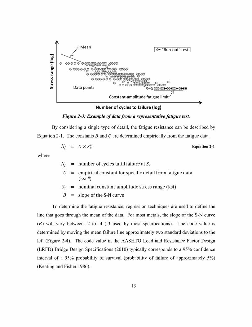
13

Figure 2-3: Example of data from a representative fatigue test.

By considering a single type of detail, the fatigue resistance can be described by

Equation 2-1. The constants and are determined empirically from the fatigue data.

Equation 2-1

where

numberofcyclesuntilfailureat

empiricalconstantforspecificdetailfromfatiguedataksi‐B

nominalconstant‐amplitudestressrange ksi

slopeoftheS‐Ncurve

To determine the fatigue resistance, regression techniques are used to define the

line that goes through the mean of the data. For most metals, the slope of the S-N curve

( ) will vary between -2 to -4 (-3 used by most specifications). The code value is

determined by moving the mean failure line approximately two standard deviations to the

left (Figure 2-4). The code value in the AASHTO Load and Resistance Factor Design

(LRFD) Bridge Design Specifications (2010) typically corresponds to a 95% confidence

interval of a 95% probability of survival (probability of failure of approximately 5%)

(Keating and Fisher 1986).

Stre

ss r

ange

(lo

g)

Number of cycles to failure (log)

Mean

Data points

Constant-amplitude fatigue limit

“Run-out” test

14

Figure 2-4: Regression lines from a representative fatigue test.

As shown in Figure 2-3, there is a stress range at which the detail is assumed to

have an infinite fatigue life for a given constant-amplitude stress range. This horizontal

line corresponds to the constant-amplitude fatigue limit (CAFL). The determination of

the CAFL historically corresponded to two million cycles, at which point the specimen

would be declared a “run-out” test. The two-million cycle limit was based upon

equipment limitations during the period of testing (1970s-1980s) (Munse 1964). With

modern testing facilities, specimens can be and are often tested to much higher cycle

counts.

The equation currently used in the AASHTO LRFD Specifications (2010) is

shown in Equation 2-2. As expected, the form follows Equation 2-1, with the exception

that all detail categories are assumed to have a value of equal to -3. Because Equation

2-2 is used for design, the fatigue constant ( ) for each fatigue category reported in Table

2-1 are lower-bound values (approximately 5% probability of failure).

Equation 2-2

where

numberofcyclesuntilfailureat

fatigueconstantfordetailcategory,definedbyAASHTO

Stre

ss r

ange

(lo

g)


Code value

Constant-amplitude fatigue limit

5% probability of failure

95% probability of survival

Number of cycles to failure

PDF

Mean

15

LRFDSpecifications 2010 ksi3

constant‐amplitudestressrange ksi

Table 2-1: Fatigue constant ( ) and constant-amplitude fatigue limit (CAFL) for each

fatigue detail category (AASHTO LRFD Specifications 2010)

Category Fatigue constant, (ksi3) CAFL (ksi) A 250×108 24.0 B 120×108 16.0 B′ 61×108 12.0 C 44×108 10.0 C′ 44×108 12.0 D 22×108 7.0 E 11×108 4.5 E′ 3.9×108 2.6

The AASHTO fatigue categories for design are best understood by graphing the

expressions in the form of S-N curves as shown in Figure 2-5. The AASHTO LRFD

Specifications (2010) provide examples of typical types of details that fit into each of the

eight fatigue categories. For instance, Category A corresponds to the fatigue resistance

of the base metal (i.e. flat plate with no weld attachments) and Category B corresponds to

continuous longitudinal fillet welds. The specimen from Figure 2-1(a) would be

considered a Category A detail. Because the CAFL are high and the fatigue constants are

so large, these types of details never control the fatigue resistance of a bridge. Instead,

the design of details with discontinuities or attachments with fillet or groove welds

parallel and perpendicular to the applied stress are more likely to be controlled by fatigue

considerations. In those situations, the fatigue category varies between C and Eʹ. The

specimen Figure 2-1(c) could be classified as a Category E detail, whereas the

classification of specimen from Figure 2-1(b) would depend on the radius of the

transition.

16

Figure 2-5: AASHTO S-N curves for design of steel bridges.

2.2.1.1 Palmgren-Miner’s Rule

Though fatigue tests have historically been performed using a constant-amplitude

stress range, real structures are subjected to varying-amplitude stress ranges. For bridges,

the amplitudes vary with the weight and length of the crossing vehicles. For offshore

structures, the amplitudes depend on the wave height and frequency. Though one event

may generate a 5-ksi cycle and the next event produces a 3-ksi cycle, each will contribute

to the fatigue damage.

A cumulative damage theory is needed to relate the varying-amplitude cycles to

the constant-amplitude fatigue data. Palmgren-Miner’s rule is the most commonly-used

cumulative damage theory because it is simple and agrees well with historic fatigue data

(see Section 2.3.1). The rule follows a linear-damage hypothesis and is expressed by

Equation 2-3 and Equation 2-4 (Miner 1945).

,

Equation 2-3

Equation 2-4

1

10

100

1E+05 1E+06 1E+07 1E+08

Stre

ss r

ange

, Sr

(ksi

)

Number of cycles to failure, Nf

ABB′

C & C′D

EE′

C′ C

17

where contributionofcycles toPalmgren‐Miner’sdamage

accumulationindex

Palmgren‐Miner’sdamageaccumulationindex numberofcyclesmeasuredat ,

, numberofcyclesuntilfailureat , numberofdifferentstressranges

In Palmgren-Miner’s rule, each cycle causes damage; however, the damage

induced is proportional to the number of cycles corresponding to failure for the actual

stress range. The total damage in an element subjected to multiple stress ranges can be

determined by simply summing the damage that accumulates at each stress range. For

example, considering a detail with an AASHTO Category D rating that is tested for

300,000 cycles at 8 ksi and 300,000 cycles at 16 ksi, the damage at each stress range can

be evaluated and summed. As shown in Figure 2-6, although the number of cycles are

the same for the two stress ranges, the 16-ksi cycles contribute eight times as much

damage as compared to the 8-ksi cycles. The reason for the difference is because , is

inversely proportional with the cube of the stress range.

Figure 2-6: Example of damage accumulation index.

0

500,000

1,000,000

1,500,000

2,000,000

2,500,000

3,000,000

3,500,000

4,000,000

4,500,000

8 16

Nu

mb

er

of

cycl

es

Stress range (ksi)

4.3x106

cycles at 8 ksi

0.54x106

cycles at 16 ksi

0.3x106

0.0

0.1

0.2

0.3

0.4

0.5

0.6

0.7

0.8

0.9

1.0

8 16

Dam

age

accu

mu

lati

on

ind

ex

Stress range (ksi)

0.07

0.56

18

The two stress ranges considered in Figure 2-6 can be converted to a single,

equivalent stress range using the concept of an effective stress range. While summing the

damage for the two stress ranges discussed above is relatively simple, in actual bridges

the stress ranges have a wide variation such that combining the damage from cycles at

many stress ranges is not practical. An effective stress range relates the damage caused

by many variable-amplitude stress ranges to a constant-amplitude stress range. Because

the distribution of stress ranges is condensed into the effective stress range, it is a more

practical design solution.

If Equation 2-2 is combined with Equation 2-4, the damage from a spectrum of

stress ranges (left side) must equal the damage from a single, effective stress range (right

side) as seen in Equation 2-5. The effective stress range ( can then be determined by

Equation 2-6. As is discussed in Section 2.3.1, the effective stress range can be used

directly with the AASHTO S-N curves.

, Equation 2-5

,

/

,

/

Equation 2-6

where

effectivestressrange ksi

totalnumberofcyclesmeasured

ratioof to

For the example in Figure 2-6, the effective stress range is 13.2 ksi for the

600,000 stress cycles. Due to the cubing term on the stress range, the effective stress

range is weighted more towards the 16-ksi stress range. If a different distribution of

cycles were used to produce the same damage accumulation index, the effective stress

range will change for the given number of cycles. For example, as shown in Figure 2-7,

if there were only 100,000 cycles at 16 ksi and 1,900,000 cycles at 8 ksi, the damage

19

index (0.63) is the same as the previous example (Figure 2-6); however the effective

stress range is 8.84 ksi for 2,000,000 cycles. Therefore, the effective stress range varies

depending on the number of measured cycles, even if the damage level is the same.

The two examples outlined above produce the same amount of damage; however,

the effective stress ranges are quite different. As such, the effective stress range by itself

is not a reliable indication of damage; two effective stress ranges cannot be compared

with one another to determine the amount of damage. Rather, the effective stress range

must be considered along with the number of cycles to make the comparison.

Figure 2-7: Revised example of damage accumulation index.

According to Palmgren-Miner’s rule, failure is assumed to occur when 1.0.

Due to the scatter in measured fatigue data, failure can occur at a damage accumulation

index that varies considerably from 1.0. The value of the damage accumulation index

corresponding to failure would be 1.0 if the actual number of cycles to failure for each

stress range were known for the connection beforehand (Equation 2-4). Instead, the

number of cycles corresponding to failure used in these calculations is based on the

lower-bound and/or average values from tests of typical connection details within the

fatigue category. For a test with two different stress ranges, the damage can be reflected

by Equation 2-7 (Tanaka and Akita 1975).

0

500,000

1,000,000

1,500,000

2,000,000

2,500,000

3,000,000

3,500,000

4,000,000

4,500,000

8 16

Nu

mb

er

of

cycl

es

Stress range (ksi)

0.0

0.1

0.2

0.3

0.4

0.5

0.6

0.7

0.8

0.9

1.0

8 16

Dam

age

accu

mu

lati

on

ind

ex

Stress range (ksi)

4.3x106

cycles at 8 ksi

0.54x106

cycles at 16 ksi

0.1x106

1.9x106

0.44

0.19

20

, ,

Equation 2-7

where

, averagenumberofcyclesuntilfailurefor ,

numberofcyclesmeasuredat ,

Equation 2-7 can be rewritten slightly as shown in Equation 2-8.

,

,

, ,

,

,∆

, , Equation 2-8

where

,

,

Palmgren‐Miner’scriticaldamageindex,ratioofnumberofcyclesuntilfailureofspecimentoaveragenumberofcyclesuntilfailurefor ,

The uncertainty from using Palmgren-Miner’s rule can be encapsulated in the

critical damage index ( ). If the mean S-N curves are used to determine , , the value

of is expected to have a mean of 1.0. After reviewing data from over a thousand tests

of welded connections, a lognormal distribution with a median of 1.0 and coefficient of

variation of 65% was recommended for the critical damage index (ASCE 1982).

However, some of the data included in the review were from small-scale tests, which had

higher variability than full-scale tests. For fatigue in offshore structures, the critical

damage index is modeled by a lognormal distribution with a median of 1.0 and

coefficient of variation of 30%, which is based on a survey of fatigue tests of structural

sections (Wirsching 1984). For most tests of offshore fatigue details, the median is 1.0

and the coefficient of variation ranges between 30-60% (Wirsching and Chen 1988).

2.2.1.2 Cycle-Counting Methods

To use Palmgren-Miner’s rule, the stress spectrum must be determined. If field

measurements are utilized, a cycle-counting method is needed to transform the stress

21

history into a histogram of stress amplitudes. Four types of counting methods for fatigue

analysis are included in ASTM E1049 (2011): (1) level-crossing counting, (2) peak

counting, (3) simple-range counting, and (4) rainflow counting or related methods. The

various methods will produce different stress spectrums for a given stress history; thus,

each method should be validated with Palmgren-Miner’s rule and fatigue data (S-N

curves).

A simplified rainflow method is considered to be well-suited for fatigue analyses

(Dowling 1972), and differs slightly from the rainflow method in ASTM E1049 (2011).

In the ASTM rainflow method, half cycles are counted; whereas, the simplified rainflow

method resolves everything in a stress history into full cycles. The method is outlined by

Downing and Socie (1982), and the analysis can be performed in real time or offline. If

the simplified rainflow method is used to determine amplitudes of cycles and the cycles

are transformed into an effective stress range using Palmgren-Miner’s rule, the results

have matched historic S-N curves (Swenson and Frank 1984).

The simplified rainflow method can be applied to a strain/stress history, such as

the one in Figure 2-8. The first step of the method is to identify all of the relative peaks

and valleys (the black dots). Next, the history has to be re-ordered to find the maximum

stress (point A). All data points that occur prior to the maximum are moved to the end of

the stress history.

The peaks and valleys shown in Figure 2-8 were re-ordered as shown in Figure

2-9(a). A full cycle is counted when a hysteresis has been formed by three data points.

For example, consider the three data points A, B, and C in Figure 2-9(a). The stress

difference between data points A and B is designated as stress range “Y” while the stress

difference between data points B and C is designated as stress range “X.” If Y is equal to

or less than X, the range is counted and the data points associated with the counted range

(Y) are discarded. If Y is greater than X, the next data point is considered (i.e., data point

D). New data points are considered until all ranges have been counted (i.e. there are no

longer three data points).

22

Figure 2-8: Stress history for example of simplified rainflow counting.

Figure 2-9: Step-by-step procedure for simplified rainflow counting.

-6.0

-4.0

-2.0

0.0

2.0

4.0

6.0

0 1 2 3 4

Stre

ss (

ksi)

Time (sec)

0.75

0.5

0.25

0.5

11

A

B

C

DF

G

H

I

JE

Summary:(1) 0.25-ksi cycle(2) 0.5-ksi cycles(1) 0.75-ksi cycle(1) 11-ksi cycle

-6.0

-4.0

-2.0

0.0

2.0

4.0

6.0

Stre

ss (

ksi)

-6.0

-4.0

-2.0

0.0

2.0

4.0

6.0

Stre

ss (

ksi)

A

B

C

D

E

F

G

H

I

J

A

Count CD = 0.5 Count EF = 0.5

Count GH = 0.75

Count IJ = 0.25

Count AB = 11

(a) (b)

(c) (d)

A

B

G

H

I

J

AA

B

I

J

A

A

B

E

F

G

H

I

J

A

23

The rules for the method can be followed in Figure 2-9. In part (a), the first time

that Y is less than X is when data points C-E are considered; Y (CD) would be counted

with a stress range of 0.5 ksi and those points discarded. The process continues in part

(b) when Y (EF) is less than X (FG) for another stress range of 0.5 ksi. Cycle GH is the

next stress range counted (part (c)) at 0.75 ksi. Finally, in part (d), cycles IJ (0.25 ksi)

and AB (11 ksi) are counted and all cycles have been counted for the example stress

history.

2.2.2 Linear-Elastic Fracture Mechanics

Fatigue resistance can also be characterized by fracture-mechanics principles.

Fracture-mechanics methods are not used as often as a stress-range model (S-N curves);

however, fracture mechanics provides more insight into the fatigue problem because the

propagation of cracks until fracture can be calculated. In the stress-based approach, only

the number of cycles until failure is determined. In a fracture-mechanics approach, the

initial flaw size and fracture toughness are included in the analysis of fatigue resistance.

The linear-elastic fracture mechanics (LEFM) method is the most common approach to

engineering problems. This approach assumes small displacements, that the material is

isotropic and linear elastic, and that a small plastic zone exists at the crack tip. The

method is mainly an analytical approach; however, some empirical tests are needed to

determine correction factors.

The most common fracture-mechanics model relates the fracture toughness of a

material to the applied stress ( ) and crack length ( ). The stress intensity factor ( ) is

used as a measure of the fracture toughness of the material. The value varies with

temperature and is difficult to determine experimentally. However, the Charpy V-notch

test can be used to indicate fracture toughness. It only provides a qualitative approach

because stress and crack length values are not assessed directly (Fisher, Kulak, and Smith

1998). The stress intensity factor can be calculated using Equation 2-9.

√ Equation 2-9

24

where

stressintensityfactor ksi√in.

correctionfactorfornon‐uniformlocalstressfields

correctionfactorforplateandcrackgeometry

appliedstress ksi

cracklength in.

The correction factors in Equation 2-9 can be determined empirically or through

numerical methods. The results are summarized in fracture mechanics handbooks, such

as Barsom and Rolfe (1999).

Equation 2-9 can be modified for specimens subjected to fatigue loading, as seen

in Equation 2-10.

∆ ∆ √ Equation 2-10

where

∆ stressintensityfactor range ksi√in.

∆ appliedstressrange ksi

Equation 2-10 can be related empirically to the crack-growth rate ( / ) which

is obtained from the slope of the curve of crack-growth measurements. If that is done,

the results can be plotted on a log-log plot (Figure 2-10). From the tests, there is a region

where cracks do not grow or the cracks grow at a very slow rate (Region I). The region

corresponds to the threshold of the stress intensity factor range ( ). In Region III,

crack growth accelerates very rapidly until fracture occurs. As such, the region intersects

with the fracture toughness of the material ( ). Region II corresponds to the propagation

of the crack. Paris, Gomez, and Anderson (1961) proposed an equation to relate the

crack-growth rate to the stress intensity factor range (Equation 2-11). The equation is

commonly referred to as Paris’ law.

25

Figure 2-10: Change in crack-growth rate, / , with range of stress intensity

factor.

∆ Equation 2-11

where

materialconstantfromregressionanalysisoftestdata

upperboundisapproximately3.6 10 √ .forbridgesteelsandweldedconnections Fisher,etal.1993

materialconstantfromregressionanalysisoftestdatatypically3.0forsteelstructures

If Equation 2-11 is rearranged and integrated, the number of cycles until failure

can be determined. If Equation 2-10 is also substituted, the result is Equation 2-12.

1 1

∆1 1

∆ √ Equation 2-12

where

numberofcyclestofailure

criticalcracklength in.

initialcracklength in.

log

da

/dN

log ΔK

log

da

/dN

log ΔKΔKth KI

Reg

ion

I

ΔKth KI

Idealized

Actual

Fracture toughness

Reg

ion

II

Reg

ion

III

(b)(a)

26

With Equation 2-12, the parameters affecting the number of cycles until failure

can be evaluated. The impact of changing the critical crack length, initial crack length,

stress range, and type of detail are shown in Figure 2-11. As shown in Figure 2-11(a),

increasing the critical crack length, or improving the fracture toughness of a material, has

a slight effect on fatigue strength. Doubling the critical crack length does not necessarily

double the number of cycles until failure because the crack-growth rate increases rapidly

as the material approaches its fracture toughness. A bigger benefit can be realized by

reducing the initial crack length, or reducing the initial flaw size of a material, as shown

in Figure 2-11(b). Such a small change in the initial flaw size produces a great increase

in number of cycles until failure. The large scatter in the fatigue data in the S-N curves

could partly be attributed to differences in the initial flaw size. Though tests performed at

the same time would be expected to have similar flaw sizes, differences in groups of tests

could be attributed to the initial flaw size. As expected, reducing the stress range will

increase the number of cycles until failure (Figure 2-11(c)). Finally, changing the fatigue

category would lead to different values for and in Equation 2-9, which could

improve the fatigue life (Figure 2-11(d)). Any or all of these methods can be used to

impact the fatigue life.

The LEFM approach is not often used due to the limitations of the method.

Mainly, controlling and/or determining the initial crack size is difficult, and as shown in

Figure 2-11(b), it has a significant impact on fatigue life. In addition, estimating the

stress intensity factor range for complex geometric shapes (finding and ) makes the

method impractical for design.

27

Figure 2-11: Change in number of cycles due to change in (a) critical crack length, (b)

initial crack length, (c) stress range, and (d) type of detail.

2.3 LITERATURE REVIEW

A literature review in three areas is presented below. The first area summarizes

the research on the response and behavior of steel structures subjected to variable-

amplitude loading (Section 2.3.1). The uncertainties that encompass monitoring bridges

in the field for fatigue evaluation are discussed in Section 2.3.2. Finally, the concepts of

structural reliability and the application of probabilistic approaches to estimating

remaining fatigue life are presented in Section 2.3.3.

Cra

ck le

ngt

h

Number of cycles

Cra

ck le

ngt

h

Number of cycles

Cra

ck le

ngt

h

Number of cycles

Cra

ck le

ngt

h

Number of cycles

ac,1ac,2 Change in critical

crack length

Change in number of cycles

Nf,2 Nf,1

ai

ac

Change in initial crack length


Nf

ai,1ai,2

(b)(a)

(c)

ac

aiNf,1 Nf,2


Higher stress range

Lower stress range

Nf,1Nf,2

ac

ai

Base detail category

Better detail category


(d)

28

2.3.1 Development of Fatigue Resistance Under Variable-Amplitude Loading

Prior to 1970, the fatigue guidelines in the AASHTO LRFD Specifications were

based on small-scale specimens that were tested at constant-amplitude loading.

However, bridges are subjected to variable-amplitude cycles from vehicles of varying

weights crossing the bridge. Thus, in the 1970-1980s, National Cooperative Highway

Research Program (NCHRP) sponsored a series of projects to determine the fatigue

resistance of various details used in bridges under variable-amplitude loading. The

fatigue behavior under variable-amplitude loading is summarized below. Except where

noted, all fatigue tests were performed on beam elements with a constant-moment region.

2.3.1.1 NCHRP Project 12-12

NCHRP Project 12-12 investigated the effects of variable-amplitude loading on

fatigue life under simulated traffic loading (Schilling, et al. 1978). The researchers found

that the variable-amplitude data could be related to the constant-amplitude data using an

effective stress range concept. It was also observed that the primary variables affecting

variable-amplitude loading were the same as the variables affecting constant-amplitude

loading.

Previous variable-amplitude fatigue tests utilized block loading. The block

loading consisted of organizing the sequence of loads in a fixed sequence that was often

very different from random traffic. In this study, the specimens were loaded following a

Rayleigh probability-density function, which is defined by two variables: (1) modal stress

range ( ) and (2) dispersion ratio ( / ) (Figure 2-12).

The researchers reviewed 51 sets of data from 37,000 truck passages to determine

the impact of a truck passage. Most truck passages at bridges produce a major stress

cycle with smaller vibrational stresses, as shown in Figure 2-13. From the data analysis,

the researchers determined that the vibrational stresses were small enough to be

neglected. As such, only major cycles were applied to the test specimens.

29

Figure 2-12: Probability of occurrence

Figure 2-13: Example truck passage

Over 300 specimens were tested during the study to understand the fatigue

behavior under variable-amplitude loading for two types of steels, A514 and A36. To aid

in planning subsequent beam tests and to study secondary test parameters, 84 small-scale,

plate specimens with a simulated cover plate were tested first in an axial setup.

Fabricated beams were then tested, with and without welded cover plates. The flange

0.0

0.1

0.2

0.3

0.4

0.5

0.6

0.7

0.8

0.9

0 2 4 6 8 10

Pro

bab

ility

of

occ

urr

ence

Stress range (ksi)

= 0.25

= 0.5

= 1.0

-3.0

-2.0

-1.0

0.0

1.0

2.0

3.0

0 1 2 3 4

Stre

ss (

ksi)

Time (sec)

Main stress cycle

Vibrational stress cycles

30

plates (6 ¾-in. width) were welded to web plates (25-in. deep) to fabricate the I-shaped

beams. A total of 156 beams with partial-length cover plates were tested to obtain the

lower bound of the fatigue strength under variable-amplitude loading (Figure 2-15).

Sixty-three beams without cover plates were tested to obtain the upper bound of the

fatigue strength.

Figure 2-14: Comparison of cover-plate beam results with AASHTO allowable stress

for Category E (from Schilling, et al. (1978))

To relate the variable-amplitude fatigue data to the constant-amplitude fatigue

data, an effective stress range concept was used (Equation 2-13).

,

/

Equation 2-13

where

proportionofcyclesatstressrange ,

fitofeffectivestressrangedata

31

Values of 2 (root mean square, RMS) and 3 (Palmgren-Miner’s rule)

were considered to fit the variable-amplitude data to the constant-amplitude data. If

3, the effective stress range from Equation 2-13 matches the stress range from

Palmgren-Miner’s rule because three corresponds to the assumed slope of the S-N curve.

The researchers found that the RMS fit the data slightly better than Palmgren-Miner’s

rule. However, Palmgren-Miner’s rule was recommended because it is more

conservative (maximum difference is approximately 11%) than RMS and the engineering

community have accepted the rule.

The primary variables affecting the fatigue resistance were ascertained from the

tests to be the stress range and type of detail. The conclusion matches the primary

variables discovered from historic, constant-amplitude fatigue tests (Schilling, et al.

1978). The minimum stress and type of steel had similar effects as reported in NCHRP

Report 12-7 (Fisher, et al. 1970; Fisher, et al. 1974) for constant-amplitude loadings and

were considered secondary parameters from that report.

By transforming the variable-amplitude data into an effective stress range, the

researchers found that the differences in the constant-amplitude and variable-amplitude

data were not statistically significant. As such, the fatigue strength of specimens subject

to variable-amplitude loading could be determined from the constant-amplitude tests.

2.3.1.2 NCHRP Project 12-15(4)

NCHRP Project 12-15(4) considered the effect on fatigue if the majority of the

cycles were less than the constant-amplitude fatigue limit (CAFL) (Fisher, Mertz, and

Zhong 1983). The results from the tests performed in this project established the

conditions under which cycles below the CAFL contribute to fatigue damage. The

frequency of occurrence above CAFL and the magnitude of the peak stress range were

both investigated.

Eight, full-size specimens (W18x50 rolled beams) were used to test gusset-plate

attachments and cover plates in fatigue. The beams were subjected to a variable-

32

amplitude stress range using a Rayleigh distribution, with stress widths ( , ,

,) of

3.75, 4.0, 4.75, and 4.75 (the stress width of NCHRP Project 12-12 (Schilling, et al.

1978) was approximately 4.67). The stress range of the variable-amplitude input

exceeded the CAFL from 0.0 to 10.16 percent of the time. As seen in Figure 2-15, three

cases were considered: (1) the effective stress range ( ) and the maximum stress range

( , ) were above CAFL, (2) the maximum stress range was above CAFL and the

effective stress range was below CAFL, and (3) the maximum stress range and effective

stress range were below CAFL.

Figure 2-15: The variable-amplitude loading cases considered in NCHRP Project 12-

15(4) (Fisher, Mertz, and Zhong 1983).

The tests revealed that as long as a portion of the applied stress was above the

CAFL (Cases 1 and 2), fatigue cracking occurred at both the web attachments and the

cover plates. If none of the cycles were above the CAFL (Case 3), fatigue cracking did

not occur. It was found that the fatigue life could be calculated using a straight-line

extension of the S-N curve for the detail, which suggests that all of the stress cycles

contribute to the fatigue damage. The scatter in the test data from using the straight-line

extension is similar to the scatter from constant-amplitude tests.

Stre

ss r

ange

(lo

g)

Number of cycles (log)

Extension of S-N curve

Constant-amplitude fatigue limit (CAFL)

Constant-amplitude S-N curve

Case 2

Case 3

Case 1

33

2.3.1.3 Swenson & Frank

A study at the University of Texas at Austin examined the influence of small

stress cycles upon the fatigue life of welded components (Swenson and Frank 1984).

After reviewing truck histories, the researchers determined that the minor cycles may

increase the fatigue damage by as much as 15% in medium-span girder bridges. The

truck histories were also used to create a variable-amplitude loading scheme for

laboratory tests, which found that all cycles in a stress spectrum are damaging. The

specimens were two plates welded together to form a tee section. The flange of the tee

section was bolted to a reaction wall and load was applied at the tip of the web (cantilever

loading).

The researchers considered four different methods for counting varying-amplitude

cycles: peak counting, range counting, simplified rainflow counting, and reservoir

counting. Simplified rainflow counting and reservoir counting produced the same stress

spectrum and were observed to be the most appropriate methods for counting cycles.

When the simplified rainflow algorithm was used to count varying-amplitude cycles and

Palmgren-Miner’s rule was applied to determine an effective stress range, the results of

the fatigue tests matched historic constant-amplitude fatigue tests.

2.3.1.4 ASCE Committee on Fatigue and Fracture Reliabilty

The American Society of Civil Engineering (ASCE) Committee on Fatigue and

Fracture Reliability published a state-of-the-art review of fatigue and fracture reliability

in 1982. One of the articles focused on variable-amplitude loading for fatigue specimens.

To relate variable-amplitude loading to constant-amplitude tests, the cycles must be

correctly identified by a cycle-counting method and then evaluated using a cumulative

damage theory.

As discussed in Section 2.2.1.1, the most commonly-used cumulative damage

theory is Palmgren-Miner’s rule. The damage theories were most useful before the

development of fracture-mechanic models provided better mathematical models of crack-

growth data; however, the theories remain useful today due to their simplicity.

34

Palmgren-Miner’s rule is a linear damage hypothesis that is simple in application: the

rule does not agree with all experimental data. For instance, Palmgren-Miner’s rule is not

very accurate if the load sequence or mean stress are important variables in the fatigue

behavior. Load sequencing and mean stress are typically not important in situations

where there is significant inelastic behavior at all strain levels. As mentioned before,

welding creates significant residual stress, which causes inelastic behavior at low stress

levels.

The variability in using Palmgren-Miner’s rule was evaluated by reviewing data

from eleven researchers and over a thousand laboratory tests. Based on that data, a

lognormal distribution with a median of 1.0 and coefficient of variation of 65% was

suggested to characterize the variability in using the rule. However, some of the data

included in the review were from small-scale tests, which had higher variability than full-

scale tests. Despite the limitations of Palmgren-Miner’s rule, it continues to be used

because of its simplicity and because other damage theories, whether linear or nonlinear,

have not proven to provide consistently better results.

The committee recommended use of the simplified rainflow method because it

can lead to a better prediction of fatigue life (Dowling 1972). The simplified rainflow

method is considered superior to other methods because it identifies stress ranges

associated with closed-loop hysteresis, which is compatible with constant-amplitude

fatigue data.

2.3.1.5 NCHRP Project 12-15(5) – Fatigue Database

NCHRP projects from 1966 to 1972 formed the basis of the 1974 AASHTO

fatigue specification (Keating and Fisher 1986). Over 800 constant-amplitude, full-sized

fatigue tests were used to define the S-N curves. Due to the large number of tests

performed since then, part of the objective of NCHRP Project 12-15(5) (Keating and

Fisher 1986) was to review and expand the current fatigue database.

Past NCHRP research had shown that the fatigue data (stress range versus number

of cycles) can be represented on a log-log graph. The fatigue data can be assumed to

35

follow the form of Equation 2-14. The results of a regression analysis performed on the

1974 fatigue data are summarized in Table 2-2 (each fatigue category had a different

slope ( )).

log log log Equation 2-14

where

log thelog ‐axisinterceptofthelogS‐Ncurve

slopeoftheS‐Ncurve

Table 2-2: Regression analysis coefficients for AASHTO curves in 1974 (Keating and

Fisher 1986).

Category Slope,

Intercept

(mean), Standard

deviation, Intercept (lower)

A 3.178 11.121 0.221 10.688 B 3.372 10.870 0.147 10.582 C 3.25 10.038 0.063 9.915 D 3.071 9.664 0.108 9.453 E 3.095 9.292 0.101 9.094 E′ 3.00 -- -- 8.61

Data from several sources including the United States, Japan, Germany, Canada,

and The Office of Research and Experiments of the International Institute of Technology

(ORE), were evaluated and added to the fatigue database, expanding the database to

nearly 2,000 tests. Based on the updated data, the slope ( ) of all of the fatigue

categories became -3.0 and another category was added to the list of S-N curves. The

authors determined that the distribution of initial flaws, residual stress fields, and

specimen size played a major role on which data sets were grouped together. The initial

size of the flaw was of particular importance, which matches the results of the fracture-

mechanics approach to fatigue evaluation (Figure 2-11).

The researchers proposed a design equation that is used in the modern AASHTO

fatigue code (Equation 2-2). The proposed values of the lower-bound fatigue constant

36

( ) for each fatigue category are listed in Table 2-3 and are approximately the same

values used in the current AASHTO LRFD Specifications (2010) (Table 2-1).

Table 2-3: Proposed lower-bound fatigue constant (Keating and Fisher 1986).

Category Fatigue constant, (ksi3) A 2.500×1010

B 1.191×1010 B′ 6.109×109 C 4.446×109 D 2.183×109 E 1.072×109 E′ 3.908×108

2.3.1.6 NCHRP Project 12-28(03)

The objective of NCHRP Project 12-28(03) was to develop more accurate

procedures for evaluating existing bridges and designing new bridges for fatigue (Moses,

Schilling, and Raju 1987). The method for estimating the remaining fatigue life was

developed considering realistic bridge conditions and a probabilistic model for analysis.

The method developed by the researchers was published by AASHTO as the Guide

Specifications for Fatigue Evaluation of Existing Steel Bridges (1990).

The procedure provided engineers with realistic values to model fatigue

conditions and estimate the remaining fatigue life for bridges. The authors evaluated

bridge data and past research to recommend values for the weight and axle spacing of the

fatigue truck (Figure 2-16), presence of multiple trucks on a bridge ( , dynamic impact

( , moment range ( , lateral distribution ( , member section ( , reliability

factors, cycles per truck passage ( ), and lifetime average truck volume. The fatigue

truck is based on weigh-in-motion data from 30 sites nationwide and 27,000 observed

trucks. The fatigue truck is expected to produce a similar amount of fatigue damage on

average as the typical assortment of trucks at a site. If the site-specific distribution of

weights of trucks is known, the weight of the fatigue truck ( ) can be modified using

Equation 2-15. Otherwise, a gross weight of 54 kips can be assumed. Based on the

37

weigh-in-motion data, the maximum weight of a single truck is expected to be twice as

much as the fatigue truck. Though, that truck would rarely cross a given bridge.

Figure 2-16: Dimensions and distribution of weight of fatigue truck.

/

Equation 2-15

where

weightofthefatiguetruck kips

frequencyofgrossweightswithininterval

grossweightoftruckswithininterval kips

The design stress range for fatigue can be calculated using Equation 2-16. The

values recommended by the authors for , , , and are not as conservative as

might be used to check the flexural capacity because fatigue is an averaging process; one

vehicle will not cause fracture, but thousands to millions will. The authors also suggest

how to modify the section modulus ( ) to account for unintended composite action.

Equation 2-16

where

momentrangecausedbypassageofthefatiguetruck

sectionmodulus

lateralgirderdistribution

impactfactor

30′-0″ 6′-0″14′-0″

6 kips 24 kips 24 kips W = 54 kips

38

multiplepresencefactor

cyclespertruckpassage

A fatigue reliability model was created to provide a consistent safety margin

(Equation 2-18). If 0, failure is assumed to occur.

Equation 2-17

where

ageofbridgeatwhichfailureoccurs randomvariable

ageofbridge deterministic

The age of the bridge at which failure occurs ( ) depends on a number of

variables. The uncertainty of each variable can be modeled and normalized to determine

the reliability factor ( ) of the suggested equation for the remaining fatigue life. A

lognormal distribution was used for each random variable in Equation 2-18.

P Z 0 P365

0 Equation 2-18

where

numberofstresscycles deterministic

ageofbridge deterministic

reliabilityfactor tobedetermined

Palmgren‐Miner’srule 1.0,COV 15%

normalizedmomentrange 0.97,COV 3%

normalizedgrossweightoftheequivalentfatiguetruck1.0,COV 10%

multiplepresenceoftrucksonthebridge 1.03,COV 0.6%

impactfactor 1.0,COV 11%

girderlateraldistributionfactor 1.0,COV 13%

normalizedeffectivesectionmodulus 1.0,COV 10%

equivalentnumberofstresscyclesduetosingletruckpassage1.0,COV 5%

39

lifetimeaveragedailytrucktraffic 2500,COV 10%

normalizedfatigue‐strengthcurve 1.297,COV 15.3%

The means and coefficients of variation (COV) are presented for each variable.

The uncertainty in all of the variables, except for Palmgren-Miner’s rule ( , was

determined from field data. For Palmgren-Miner’s rule ( , the COV value of 15% was

estimated because there was insufficient data on the validity of Palmgren-Miner’s rule for

welded steel bridges from typical highway loadings. However, work by Fisher, Mertz,

and Zhong (1983) does validate the assumed COV. One of the most important benefits

of a reliability analysis is that it shows the interrelationship of the various conservative

assumptions that are made at each step in the design or evaluation procedure.

The reliability factors ( ) were determined from the reliability model to be 1.35

and 1.75 for redundant and non-redundant members, respectively. Using these reliability

factors and Equation 2-19, the remaining fatigue life can be estimated with a more

consistent level of reliability for the variety of bridges types. Either the safe life (2.3%

and 0.1% probability of failure for redundant and non-redundant members, respectively)

or mean life (50% probability of failure) can be calculated, depending on the parameters

used.

10

Equation 2-19

where

remainingfatiguelifeinyears

detailconstant ksi3

estimatedlifetimeaveragedailytruckvolume

stresscyclespertruckpassage

stressrange ksi

combinedreliabilityfactor

base reliability factor (same as )

40

correction if stresses are measured (0.85)

correction if site-specific truck traffic weighs less than standard fatigue truck

correction for a more accurate calculation of the lateral distribution factor

presentageofbridgeinyears

1.0forcalculatingsafelifeand2.0forcalculatingmeanlife

Due to the scatter of the fatigue data, there can be a large difference between the

calculated mean and safe lives. In an example in the report, the calculated mean life was

138 years and safe life was 14 years. A non-redundant detail was considered in the

example, which is partly why there was such a large difference between the mean (50%

probability of failure) and safe life (0.1% probability of failure). Another potential

source of error was the use of design values for the gross weight of the fatigue truck,

average daily truck traffic (ADTT), and impact factor. The uncertainty from those

variables can be minimized if strain gages were used to determine the distribution of

fatigue cycles.

2.3.1.7 NCHRP Project 12-15(5) – Variable-Amplitude Fatigue Tests

Additional tests were conducted in NCHRP Project 12-15(5) (Fisher, et al. 1993)

to supplement and verify the preliminary observations of NCHRP Project 12-15(4)

(Fisher, Mertz, and Zhong 1983). The fatigue behavior of specimens in which the

majority of the stress ranges are below the CAFL was tested.

To accomplish the objective, eight full-size welded girders (34-in. deep web plate

with 12-in. wide flange plates) with Category Eʹ web attachments and cover-plated

flanges as well as Category C transverse stiffeners and diaphragm connection plates were

subjected to long-life, variable-amplitude loading. It was found that fatigue cracking

developed at the Category Eʹ details when the CAFL was exceeded by more than 0.05%

of the stress cycles. For the Category C details, fatigue cracks did not develop unless the

peak stress range exceeded the CAFL by more than 33%. The results supported the

41

extension of the exponential S-N relationship even when the effective stress range is

below the constant-amplitude fatigue limit.

A fracture-mechanics model was developed to analyze how smaller stress cycles

contributed to fatigue damage. The analysis indicated that the contribution is dependent

on the crack-growth threshold. If the lower stress cycles are assumed to contribute to the

damage, the estimate of fatigue life is typically conservative.

For the cover-plate details (Category Eʹ) that were tested, it was recommended

that all cycles above 50% of the CAFL should be considered to cause fatigue damage.

2.3.1.8 Manual for Evaluation in AASHTO (2011)

In 2011, AASHTO released the second edition of the Manual for Bridge

Evaluation (AASHTO 2011) for evaluating fatigue in steel bridges. The method is

similar to the procedure described in NCHRP Project 12-28(03) (Moses, Schilling, and

Raju 1987); however, the updated method utilizes new formulas and values for several

parameters from the AASHTO LRFD Specifications (2010). The updated values more

accurately reflect bridge conditions. In addition, the evaluation manual utilizes updated

values for the resistance and reliability/load factors. Equation 2-20 can be used to

estimate the fatigue life. It is similar to Equation 2-19, with some of the parameters

redefined.

365

Equation 2-20

where

fatiguelifeinyears

resistancefactor

detailconstant ksi3

stresscyclespertruckpassage

averagenumberoftrucksperdayinasinglelaneaveragedovertheentirefatiguelife

stressrange ksi

42

partialloadfactor

The guide previously used (resistance parameter) and (reliability factor) in

Equation 2-19, whereas the evaluation manual used (resistance factor) and (partial

load factor) in Equation 2-20.

According to Chotickai and Bowman (2006), the updated method utilizes lower

load factors and higher resistance factors, which produces a higher probability of failure

for a calculated fatigue life (i.e. longer calculated fatigue life). The evaluation manual

does not distinguish between redundant and non-redundant details and provides three

levels of safety for the fatigue life: minimum life (design fatigue life, two standard

deviations away from the mean fatigue resistance), evaluation life (one standard deviation

away from the mean fatigue resistance), and mean life. The values for the resistance

factor ( ) and partial load factor ( ) vary with detail and desired level of safety.

2.3.1.9 Regression Values for Current AASHTO S-N Curves

The regression values for the current AASHTO S-N curves were determined by

Keating and Fisher (1986), yet the values were not published in that NCHRP report.

Instead, the values were published in a report that is no longer available (Keating, Halley

and Fisher 1986), and were later presented in Moses, Schilling, and Raju (1987). The

regression values are in terms of the mean ( ) and design ( ) stress ranges at two

million cycles for a slope ( ) of -3.0 (Table 2-4).

By rearranging Equation 2-14, the intercept of the regression equation can be

determined (Equation 2-21). By substituting the mean stress range, the mean intercept

for the fatigue constant can be calculated (Equation 2-22).

log log 2 10 3 log Equation 2-21

log log 2 10 3 log Equation 2-22

where

meanvalueofthefatigueconstant intheAASHTOLRFDSpecifications

43

designstressrangeat2x106 cyclesforeachfatiguecategory

meanstressrangeat2x106 cyclesforeachfatiguecategory

Table 2-4: Mean and design stress ranges and coefficient of variation (COV) of fatigue

data.

Category Fatigue

constant, (ksi3)

at 2x106 cycles (ksi)

at 2x106 cycles (ksi)

COV

A 250×108 33.0 23.2 21.7% B 120×108 22.8 18.1 14.1% B′ 61×108 18.0 14.5 13.2% C 44×108 16.7 13.0 15.3% C′ 44×108 16.7 13.0 15.3% D 22×108 13.0 10.3 14.2% E 11×108 9.5 8.1 9.7% E′ 3.9×108 7.2 5.8 13.2%

The standard deviation for each fatigue category can be calculated from the

coefficient of variation ( ) (Equation 2-23).

ln 1 Equation 2-23

where

standarddeviationoflog

coefficientofvariationforeachfatiguecategoryat2x106cycles

Using the regression values from Table 2-4, the regression values for log can

be calculated and are reported in Table 2-5.

44

Table 2-5: Derived values from regression model.

Category Mean of fatigue

constant, (ksi3)

Intercept (mean),

Intercept (lower),

Standard deviation of

, A 719×108 10.86 10.40 0.21 B 237×108 10.37 10.08 0.14 B′ 117×108 10.07 9.79 0.13 C 93×108 9.97 9.64 0.15 C′ 93×108 9.97 9.64 0.15 D 44×108 9.64 9.33 0.14 E 17×108 9.23 9.03 0.10 E′ 7.5×108 8.87 8.59 0.13

2.3.1.10 Summary

The following conclusions can be inferred from the literature on the development

of fatigue resistance under variable-amplitude loading.

Variable-amplitude loading tests can be related to constant-amplitude data

through the concept of an effective stress range (Schilling, et al. 1978).

Based on updated data, the slope ( ) of all of the fatigue categories was

-3.0 (Keating and Fisher 1986).

Palmgren-Miner’s rule is most often used to determine the effective stress

range due to its simplicity and has been verified by variable-amplitude

tests (ASCE 1982; Swenson and Frank 1984).

If the effective stress range is less than the constant-amplitude fatigue

limit (CAFL), fatigue failure can occur if the maximum stress range is

greater than the CAFL. However, if the maximum stress range is less than

the CAFL, fatigue failure will not occur. A straight-line extension of the

S-N curves can be used for effective stress ranges less than the CAFL

(Fisher, Mertz, and Zhong 1983; Fisher, et al. 1993).

The minor stress cycles due to the vibration of the bridge from the passage

of a truck can cause fatigue damage. As such, the minor stress cycles

45

should be counted and considered in a fatigue evaluation (Swenson and

Frank 1984).

Because the rainflow algorithm identifies stress cycles from closed-loop

hysteresis, it is the best method for determining the amplitude of cycles in

a varying-amplitude stress history (ASCE 1982; Dowling 1972). When

the rainflow algorithm is used to determine amplitudes and Palmgren-

Miner’s rule is used to calculate an effective stress range, there is good

agreement with historic constant-amplitude fatigue tests (Swenson and

Frank 1984).

There is uncertainty in using Palmgren-Miner’s rule, which must be

considered when evaluating the fatigue life of a bridge or designing details

for fatigue (ASCE 1982).

There is still uncertainty on which cycles should be considered when

evaluating fatigue damage. Some state that all cycles are damaging

(Swenson and Frank 1984), whereas others recommend that stress ranges

that are less than 50% of the CAFL can be neglected (Fisher, et al. 1993).

2.3.2 Field Monitoring of Bridges for Fatigue Evaluation

This section contains some of the approaches used by engineers and researchers to

calculate the fatigue damage when field monitoring a bridge. Some of the approaches are

not appropriate, as they ignored fatigue cycles or produced unconservative results.

Recommended techniques for a fatigue analysis of a bridge with field-monitored data are

presented in Chapter 3.

The fatigue life of a bridge may be evaluated through structural analysis and the

application of equations in the AASHTO Manual for Bridge Evaluation (2011). The

process requires an engineer to make a number of assumptions to calculate the effective

stress range. Namely, uncertainty can arise from choosing a representative truck that

causes an equivalent amount of damage as the vehicles that cross the bridge, the number

of truck passages, how load is distributed between longitudinal girders, if composite

46

action exists, and the increase in stresses due to dynamic effects. Because the geometry

and traffic patterns at each bridge are different, the uncertainty from these assumptions

may be reduced by field monitoring to determine the actual distribution of stress ranges.

Field studies are often performed on bridges that already have problems

(determine why cracks have formed) or to justify continued use of a bridge that is past its

design life. The data are useful to bridge owners as they make plans for replacement,

retrofit, or continued use of the bridge inventory, as well as bridge inspectors to help

focus efforts on critical members. In Zhou (2006), the Cleveland Central Viaduct was

monitored after 40 years of service and determined to have an infinite fatigue life due to

the low-measured stress ranges. It has often been found that the stress ranges measured

in the field are lower than the stress ranges calculated from conservative design values

(Zhou 2006).

Despite the advantages of directly measuring the spectrum of stress ranges, there

is still some uncertainty when monitoring bridges. The uncertainty can be classified into

three areas: (1) location of sensor, (2) representation (quality of data) of traffic, and (3)

interpretation of data. Some engineering judgment is required to determine the optimum

locations for the gages. If a gage is installed at a location with low stress ranges, the

bridge could be incorrectly evaluated. Zhou (2006) recommended that bridges be

analyzed before monitoring to determine the locations that are subjected to the highest

levels of stress. Inspection reports can also be used to identify locations where cracks

have been observed.

The data obtained from field monitoring is useful only if the collected spectrum of

stress ranges is representative of actual traffic. If only a few days of data are captured,

the amount of data could be overestimated or underestimated, especially if the data

includes a holiday (Fasl, et al. 2012c). Because damage will vary with the day of the

week (more damage during the weekdays as compared to the weekend), it is necessary to

capture at least a week’s worth of data to determine the average damage per day. There

can also be fluctuations in damage on a weekly basis; as such, two to four weeks are

often needed to make long-term damage projections (Connor and Fisher 2006).

47

Obtaining data beyond a month will help define the maximum stress range; however,

those large stress ranges occur with relatively low frequency and do not significantly

influence projections of damage (Connor and Fisher 2006).

The other main cause of uncertainty deals with interpretation of the data, mainly

which cycles should be considered in the fatigue analysis. A concern of any field

instrumentation involving sensors is error in the measurements due to electromechanical

noise and/or analog resolution of the data acquisition system. The electromechanical

noise cycles are fictitious stress fluctuations that do not induce fatigue damage, and

should be truncated from a fatigue analysis. Most data acquisition systems can limit

electromechanical noise to less than 10 microstrain (Connor and Fisher 2006), with many

systems limiting noise between 2-5 microstrain.

In addition to ignoring cycles from electrical noise, many researchers truncate

data at small stress ranges because those cycles are not expected to cause much damage.

Truncating cycles that are less than 25-50% of the CAFL for each fatigue category are

typically recommended (Connor and Fisher 2006; Zhou 2006). Where ignoring electrical

noise is required (not real damage), care must be taken to ensure that damaging cycles are

not truncated, even if they correspond to small stress ranges.

Part of the reason engineers truncate lower stress ranges is because the calculation

of the effective stress range (Equation 2-6) is very sensitive to the number of fatigue

cycles in each bin (Section 2.2.1.1). In most monitoring programs, a majority of the

cycles are in the first few bins due to electromechanical noise and actual cycles from light

vehicles (cars and two-axle trucks). As a result, the calculation of the effective stress

range produces a very small value if all the data were considered.

Truncating the lower cycles produced a more realistic value of the effective stress

range. A more realistic value was important when performing a fatigue evaluation using

the AASHTO Guide for Fatigue Evaluation (1990) because whether a detail had infinite

life was not dependent on the maximum-measured stress range. Instead, it was based on

whether the calculated or measured effective stress range was less than a limiting stress

48

range; a bridge connection had infinite life if Equation 2-24 was true. The combined

reliability factor ( ) was discussed in Section 2.3.1.6.

Equation 2-24

where

limitingstressrange ksi – seeTable 2-6

Table 2-6: Limiting stress range.

Category (ksi) A 8.8 B 5.9 B′ 4.4 C 3.7 C′ 4.4 D 2.6 E 1.6 E′ 0.9

Without truncating the lower stress ranges, Equation 2-24 might be satisfied for

many bridge details that actually had a finite fatigue life. In the most recent AASHTO

Manual for Bridge Evaluation (2011), the infinite fatigue life is based on the maximum-

measured stress range, rather than Equation 2-24. Using the maximum-measured stress

range as the metric for infinite fatigue life is consistent with the long-life fatigue tests

performed by Fisher, et al. (1983).

When truncating cycles, Connor and Fisher (2006) suggested that vehicles less

than 20 kips could be neglected from a fatigue analysis because those vehicles are not

included in the load spectrum used for the AASHTO LRFD Specifications (2010). This

implies that vehicles less than 20 kips are assumed to cause only a small amount of

damage. At the Patroon Island Bridge in New York, a 20-kip vehicle was used to

determine the level of truncation for each gage, ranging from 5-33 microstrain (Alampalli

and Lund 2006). At the I-95 Bridge over James River in Richmond, Virginia, a slightly

different method was employed. There, the authors truncated lower stress ranges until

the number of cycles in the stress-range histogram matched the known ADTT at the

49

bridge (each truck caused only one stress cycle) (Zhou 2006). The effective stress range

was then calculated based on the truncated histogram.

The practice of truncating load-induced stress ranges, even though they are small,

conflicts with the conclusion that all cycles can contribute to the accumulation of fatigue

damage (Swenson and Frank 1984). In most bridges, truncating lower stress ranges may

not change the calculated amount of damage because the number of cycles is also

reduced. However, in some bridges, truncating lower stress ranges can reduce the

calculated amount of fatigue damage, which will produce unconservative estimates of the

remaining fatigue life.

The last complication of data interpretation is due to the calculation of a negative

remaining fatigue life. Leander, Anderson, and Karoumi (2010) evaluated the fatigue life

of a railway bridge in Stockholm based on the Swedish Regulations for Steel Structures,

and estimated that the design fatigue life had been exceeded. When the authors evaluated

the bridge, they found that the approximately 40% of the design fatigue life was

consumed in a year (failure expected in just over two years). However, the bridge has

been in service for over 50 years with no apparent damage. The authors attributed the

negative remaining fatigue life to conservative safety margins in the code, errors due to

Palmgren-Miner’s rule, and improper classification of the detail (by changing the fatigue

constant for the detail by 100%, the damage reduced from 0.4 to 0.018 each year). This

example underlines the importance of understanding the procedure for how the fatigue

life is calculated (probability of failure for method) and dealing with uncertainty properly

(from Palmgren-Miner’s rule and other sources). To express the uncertainty in fatigue

lives, the AASHTO Manual for Bridge Evaluation (2011) provides load and resistance

factors for three levels of safety: minimum (two standard deviations from the mean),

evaluation (one standard deviation from the mean), and mean life.

2.3.2.1 Summary

The following points can be concluded from the literature on monitoring bridges

for fatigue evaluation.

50

Capturing data in the field is beneficial to bridge owners, helping them

make decisions in terms of replacement, retrofit, or continued use of the

bridge inventory. Often the stress ranges measured in the field are much

less than those predicted from code equations because the equations

cannot accurately reflect the unique geometry and traffic conditions of

each bridge (Zhou 2006).

Two to four weeks of data are needed to make long-term damage

projections (Connor and Fisher 2006).

There is a lot of confusion on how to interpret data obtained in the field.

Electromechanical noise from data acquisition systems should be ignored

from the analysis because they do not represent actual fatigue cycles.

Many engineers truncate the lower stress cycles because they can skew

(lower) the calculation of the effective stress range. As much as 25-50% of

the CAFL has been recommended (Connor and Fisher 2006). However,

by truncating the lower stress ranges, some actual fatigue damage may be

neglected from the analysis (Swenson and Frank 1984).

The procedure for calculating the remaining fatigue life should be

understood or the results from the analysis could be misinterpreted,

especially if the remaining fatigue life is negative (Leander, Andersson,

and Karoumi 2010).

2.3.3 Structural Reliability Fatigue Analysis

If the strength and loading are known exactly, establishing fatigue failure for

critical bridge connections would be very simple. However, due to uncertainty in

material strength, section dimensions, loading, and many other sources, estimating failure

is uncertain. Structural reliability is a convenient method to characterize the probability

of failure considering the uncertainty from various sources. For specimens designed for

flexure and shear, modern codes use structural reliability to determine the appropriate

safety factors on the load and resistance to provide a consistent level of reliability. The

51

reliability can be defined as the probability that failure will not occur. Reliability

concepts can be used to develop a probabilistic approach to fatigue analysis. By using

such an approach, the uncertainty inherent in fatigue is treated in a rational manner

(Chung 2004).

2.3.3.1 General Reliability Concepts

If a specimen is assumed to have a resistance ( ) and loading ( ), each with a

given mean ( and ) and uncertainty ( and ), failure is a possibility at the overlap

between the curves (Figure 2-17(a)). In this situation, failure occurs when the loading is

greater than the resistance. A possible opportunity for failure is when the resistance is

below its mean and the loading is above its mean. The probability of failure can be

formalized by defining a limit state function ( ). If the limit state is defined in

Equation 2-25, failure will occur when 0.

0 Equation 2-25

where

uncertaintymodelforthelimitstatefunctionof and withamean andstandarddeviation

uncertaintymodelfortheresistance withamean andstandarddeviation

uncertaintymodelfortheload withamean andstandarddeviation

If and are assumed to be independent, normally‐distributed random

variables,themean anduncertainty canbedeterminedforthelimitstate

function( ) using Equation 2-26 and Equation 2-27.

Equation 2-26

Equation 2-27

52

The limit state function will also be normally distributed and the probability that

failure occurs can be determined from Equation 2-28. The probability of failure can be

shown graphically in Figure 2-17(b).

0 Φ0

Φ Equation 2-28

where

Φ cumulativedistributionfunctionofastandardnormalrandomvariable

Figure 2-17: Probability density curves for (a) and and (b) .

A reliability index ( ) is often used and is related to the probability of failure ( )

using Equation 2-29 and Equation 2-30.

Φ 1 Φ Equation 2-29

Φ Equation 2-30

The reliability index and the probability of failure are inversely related to each

other; as the probability of failure decreases, the reliability index increases. A set of

Pro

bab

ility

den

sity

fu

nct

ion

Region where failure could occur

,,

(a) (b)

Pro

bab

ility

den

sity

fu

nct

ion

53

and values are summarized in Table 2-7. Typical values for probabilities of failure in

civil engineering applications range between 10-3 to 10-5, or a reliability index between

3.09 to 4.26.

Table 2-7: Equivalent probabilities of failure and reliability indexes.

Probability of failure, Reliability index, 10-1 1.2810-2 2.33 10-3 3.09 10-4 3.72 10-5 4.26 10-6 4.75

2.3.3.2 Fatigue Reliability Analysis

Due to the considerable uncertainty from fatigue, a probabilistic approach is

appropriate for estimating the remaining fatigue life. The method presented by NCHRP

Project 12-28(03) (Moses, Schilling, and Raju 1987) used a probabilistic approach to

determine the average reliability factors for different bridges and probabilities of failure.

The approach is appropriate for certain bridge conditions. Although the NCHRP

approach provides a more consistent level of reliability for the typical assortment of

bridges, a more general probabilistic approach can be used to account for uncertainty in

all variables.

The study presented by Zhao, Halder, and Breen (1994) was one of the first to

apply a general reliability approach to bridges. The authors suggested a technique to

update the reliability index using Bayesian techniques based on the results of non-

destructive inspections (NDI). Depending on whether a crack was detected (crack length

was determined or crack length was not determined because too small) or not detected

(crack was too small for NDI method), the reliability index could be updated. By

updating the reliability index, bridge owners could make decisions on the inspection

interval or whether to repair, replace, or do nothing at a bridge.

54

Recently, Chung (2004), Orcesi, Frangopol, and Kim (2010), and Bocchini and

Frangopol (2011) have utilized reliability concepts to determine the optimal schedule for

inspections. The process involves setting a target level of reliability ( ) and

optimizing the inspection interval in terms of the cost of the inspections, repairs, and

failure. The result of these analyses produces a schedule that is non-regular, rather than

the regular schedule (every two years) specified by the current inspection requirements

(USDOT 2006)).

The reliability techniques have also been used by researchers to estimate the

remaining fatigue life. Szerszen, Nowak, and Laman (1999) developed a model that

utilized weigh-in-motion stations and S-N curves developed from test data to estimate the

reliability index for a bridge in Michigan. The data were used to determine the locations

where the fatigue damage was the highest. The authors found that the strains that were

measured were rather low; as such, the reliability index and remaining fatigue life were

both large.

Kim, Lee, and Mha (2001) applied a probabilistic method to a railway bridge to

estimate the remaining fatigue life. The probabilistic model accounted for the weight of

each train and when two trains might cross over the bridge at the same time. The

remaining fatigue life determined from the probabilistic method was compared with a

simple, deterministic approach. Because the deterministic approach is for a single

probability of failure, the methods could only be compared at that single data point.

Comparing the methods, the deterministic approach was found to have 10-20% longer

estimate for the fatigue life.

Orcesi, Frangopol, and Kim (2010) estimated that the reliability index will reach 0

(corresponds to a probability of failure of 50%) at the I-39 Northbound B-35-75 Bridge

over the Wisconsin River in 2024. The authors developed probability density functions

(PDFs) of the stress-range histogram that were validated from field data to make the

estimate of the fatigue life.

55

Kwon and Frangopol (2010) developed a reliability model that accounted for

measurement errors from misalignment of the strain gages and/or data acquisition error.

The measurement error was modeled using a lognormal distribution with a mean of 1.0

and coefficient of variation of 0.03. Two bridges were considered in the paper: Neville

Island Bridge and Birmingham Bridge. At the Neville Island Bridge, no traffic growth

was considered. Using the AASHTO equations (5% probability of failure), a positive

remaining fatigue life was calculated (4 years and 29 years) for the two locations

considered; however, one of those locations had active cracks. Using a general

probabilistic approach that is discussed in the paper, the calculated life was positive (2

years) at one location and negative (-6 years) at the other. Thus, the general method

estimated that the bridge could have active cracks for a probability of failure of 5%.

In the study on the Birmingham Bridge, the bridge was expected to have an

infinite fatigue life based on the monitored data and no traffic growth. If traffic growth

was considered, then the bridge had a finite fatigue life. The stress ranges were modeled

using PDF developed from the measured data; but the authors truncated the lower stress

ranges (up to 33% of the CAFL) because the value for the effective stress range was

skewed.

Building on the study by Kwon and Frangopol (2010), Liu, Frangopol, and Kwon

(2010) created a model for using the reliability equations with field data. The monitored

data were used to validate an FEM model and the model was used to determine critical

locations. Thus, the authors used measurements from a few locations to validate a model

that could be used to evaluate the entire bridge. The authors assumed traffic growth rates

of 2% to 5% for the fatigue analysis.

2.3.3.3 Fatigue Limit State Function

In general, there are two limit state functions used by researchers (Equation 2-31

and Equation 2-32). However, if an effective stress range ( ) is used with Equation 2-2

and Equation 2-8 to determine and , both limit state functions simplify to

the same fatigue limit state function (Equation 2-33). Equation 2-33 can be rearranged so

56

that it involves only products (Equation 2-34). By modeling the equation with products,

the limit state function ( ) can be modeled by a lognormal distribution function.

0 Equation 2-31

where

uncertaintymodelforthelimitstatefunctionof and

numberofcyclesuntilfailureforagivenstressrangeresistance

numberofcyclesatbridgeatgivenstressrangesincebridgewasputinservice loading

0 Equation 2-32

where

uncertaintymodelforthelimitstatefunctionofΔand

Δ Palmgren‐Miner’scriticaldamageindex resistance

Palmgren‐Miner’sdamageaccumulationindexsincebridgewasputinservice loading

0 Equation 2-33

where

uncertaintymodelforthefatiguelimitstatefunction

ln ln 1 0 Equation 2-34

If all of the terms of Equation 2-34 are modeled with random variables, there will

be a mean ( ) and standard deviation ( ) associated with each variable. If all of the

random variables have lognormal distributions, the reliability index for the fatigue limit

state function can be determined using Equation 2-35.

3

3

Equation 2-35

57

where

parameterforthelognormaldistributionforrandomvariablethatdependsonthemean andstandarddeviationoftherandomvariable

ln2

parameterforthelognormaldistributionforrandomvariablethatdependsonthemean andstandarddeviation oftherandomvariable

ln 1

These fatigue limit state functions have been used by many researchers to

estimate the remaining fatigue life (Szerszen, Nowak, and Laman 1999; Kwon and

Frangopol 2010; Orcesi, Frangopol, and Kim 2010; Liu, Frangopol, and Kwon 2010).

2.3.3.4 Summary

The following concepts can be deduced from the literature on applying structural

reliability concepts to fatigue evaluation.

Reliability equations can be used to evaluate fatigue damage by

accounting for uncertainty from resistance and load sources in a rational

method (Chung 2004).

A general limit state function can be used with measured data to estimate

the remaining fatigue life (Szerszen, Nowak, and Laman 1999; Kwon and

Frangopol 2010; Orcesi, Frangopol, and Kim 2010; Liu, Frangopol, and

Kwon 2010).

The probabilistic approach to estimating remaining fatigue life can be a

better approach than typical deterministic approaches (Kim, Lee, and Mha

2001; Kwon and Frangopol 2010).

Truncating the spectrum of stress ranges from data is also a concern when

applying the data to reliability equations (Kwon and Frangopol 2010).

58

CHAPTER 3

Techniques for Fatigue Analysis

When analyzing data obtained from field measurements, methods are needed to

properly evaluate fatigue damage. The traditional method of converting the distribution

of stress cycles used for a rainflow analysis to an effective stress range using Palmgren-

Miner’s rule has some shortcomings. Namely, the calculation of the effective stress

range ( ) can be skewed if there is a large percentage of the cycles in the first few bins.

As such, even if two different stress spectra generate the same amount of fatigue damage,

the spectra will likely produce different values for the effective stress range.

A new method, denoted as the index stress range, was developed as part of this

research investigation. The method is targeted for evaluating and comparing fatigue

damage at multiple locations in a structural system based on rainflow data from strain

gages. The index stress range is advantageous to the effective stress range because the

extent of fatigue damage induced at the location of each strain gage is normalized.

Rather than calculating the effective stress range for a given number of cycles, the

number of equivalent cycles at an index stress range ( ) is determined for a set amount

of induced fatigue damage.

Two techniques for visualizing the influence of the stress spectrum to the fatigue

damage are also presented. The contribution to damage and cumulative damage can be

calculated for measured strain histories. Both techniques are used to characterize the

effect of cycles within specific stress ranges of the induced fatigue damage. Many

engineers truncate the cycles in the lower stress ranges of the stress spectrum because

these cycles are either attributed to electromechanical noise within the data acquisition

equipment, or the amplitude of the cycles are so low that they are assumed not to

contribute to the fatigue damage. The electromechanical noise cycles do not correspond

to stress cycles experienced by the bridge, and therefore, do not induce damage. These

cycles should clearly be truncated from a fatigue analysis. However, the low-amplitude

59

load-induced cycles should not necessarily be truncated. Truncating the cycles

corresponding to the lower stress ranges increases the calculated value of the effective

stress range for a given strain history.

At the other end of the stress spectrum, the larger stress cycles may be load

induced or caused by electromechanical spikes from lightning or radios. If a cycle was

caused by a spike in the data acquisition system, the cycle should not be included in the

fatigue analysis. Determining the cause of the large-amplitude stress cycles has

historically been very difficult; however, several approaches were used in this

investigation The consequences of truncating cycles corresponding to lower and higher

stress ranges can be assessed by plotting the contribution to damage and cumulate

damage for the stress spectra.

Data from a few strain gages at two bridges were used to demonstrate the

importance of the methods discussed in this chapter. Data from the remaining gages and

bridges are summarized in Chapter 5 and the appendices. The specific details of the

bridges are not important for the examples discussed in this chapter; however, the

structural characteristics of the bridges are described in detail in Chapter 4. Bridge A is a

statically-determinant, three-span bridge that features two longitudinal girders. Strain

gages were concentrated near the north end of the bridge, near the connections to floor

beams 34 and 35. Two gages were considered in this chapter for Bridge A: W-34s-TE

and E-34s-TE. W-34s-TE corresponds to a gage installed on the west longitudinal girder

of Bridge A near floor beam 34 on the east side of the top flange, whereas E-34s-TE

corresponds to the east longitudinal girder. Throughout this discussion, data from W-

34s-TE will be identified as the west girder and data from E-34s-TE will be referred to as

the east girder.

Bridge D is a continuous, three-span bridge with seven girders across the bridge

width. Only one gage was considered for Bridge D in this chapter and it is located on the

bottom flange of girder 3 in the middle of the center span (L1-3-BN).

60

3.1 SIMPLIFIED RAINFLOW ANALYSIS

The first step to evaluate the fatigue damage using data from field measurements

in a bridge is to determine the distribution of stress cycles. As discussed in Chapter 2, the

simplified rainflow analysis is typically used because it counts cycles due to closed-loop

hystereses (Dowling 1972).

Following the algorithm outlined by Downing and Socie (1982), the distribution

of stress cycles for a single truck event can be determined. The stress history shown in

Figure 3-1 corresponds to gage W-34s-TE for a four-axle vehicle crossing in the right

lane of Bridge A. The primary cycle has an amplitude of 3.4 ksi; however, there are

seven other smaller stress-range cycles, due to bridge vibrations, with amplitudes

between 0.4 and 1.2 ksi. By considering all eight cycles and using Palmgren-Miner’s

rule (Section 2.2.1.1), the fatigue damage was increased by 11% as compared to

considering only the primary cycle (3.4 ksi).

Figure 3-1: Example stress history at the west girder from truck event and the results

of the simplified rainflow analysis.

Rather than record each specific stress range (as in Figure 3-1), the stress ranges

are typically accumulated in rainflow bins. The rainflow bins correspond to a specific

‐2.0

-1.5

-1.0

-0.5

0.0

0.5

1.0

1.5

2.0

0 1 2 3 4 5

Stre

ss (

ksi)

Time (sec)

Summary:(2) 0.4-ksi cycles(1) 0.5-ksi cycle(2) 0.8-ksi cycles(1) 1.1-ksi cycle(1) 1.2-ksi cycle(1) 3.4-ksi cycle

11% increase in damage due to secondary cycles

61

range and make it easier to summarize the spectrum of stress ranges measured at a bridge.

An example histogram is presented in the next section.

Following the procedure outlined by Downing and Socie (1982), the simplified

rainflow method was implemented in LabVIEW for use in the research outlined in this

dissertation. LabVIEW is a graphical programming language that was developed by

National Instruments (NI). It can be used with many different computer platforms;

however, LabVIEW is ideally compatible with NI hardware.

The program can be executed offline on a Windows-based computer or in real-

time on NI hardware. The user inputs the data (strain/stress history), the size of the bins

for the histogram, the number of total bins, the minimum amplitude to count, and the

length of the analysis. The program will reduce the strain/stress history into peaks and

valleys, save the peaks and valleys into memory, and determine the amplitude of each

cycle and put it into the appropriate bin of the rainflow histogram.

If a cycle is less than the minimum specified amplitude, the corresponding peak

and valley are deleted and not counted. As such, the minimum amplitude should be set at

the limit for the expected electromechanical noise from the data acquisition system

(typically between 1-10 microstrain).

The size of the bins times the number of total bins is the total spectrum of stress

ranges for the bridge that can be identified. The required spectrum could vary for each

gage location and bridge that is monitored. As such, care should be taken to ensure that

the total spectrum is wide enough to accommodate the largest expected stress range. If a

stress range is larger than the total spectrum, it is put into the last bin; but, the actual

value for that stress range is not known. As an example, if 10 bins were specified, each

0.5-ksi wide, the total spectrum would be 5 ksi. Any cycle above 5 ksi that is captured

would be put into an 11th bin. However, the values of the cycles above 5 ksi would not

be known because the total spectrum was not large enough.

The duration of the analysis is an important consideration. If the duration is too

long, a potentially large, fictitious cycle due to the drift of the strain gage with

temperature may be counted. If the duration is too short, then the count could be biased

62

due to partial cycles being counted as full cycles. A length of 30 minutes was chosen for

all of the analyses in this dissertation. In 30 minutes, the drift of the gage due to

temperature is generally minimal and the time is long enough to provide a realistic count

(Fasl, et al. 2010).

3.2 AMOUNT OF FATIGUE DAMAGE

The primary goal of any monitoring project is to determine the amount of fatigue

damage that is induced during the monitoring period. The damage is then typically used

to estimate the remaining fatigue life by projecting damage in years prior to the

monitoring period and in the future. AASHTO LRFD Specifications (2010) relates the

number of cycles to failure for a given stress range using Equation 3-1; the equation is

often plotted and referred to as S-N curves. Thus, the fatigue damage is described by the

number of cycles times the stress range cubed, and the fatigue resistance is .

Equation 3-1

where

designnumberofcyclesuntilfailureat

fatigueconstantfordetailcategory,definedbyAASHTOLRFDSpecifications 2010

constant‐amplitudestressrange

Because bridges experience variable-amplitude stress ranges, it is useful to

transform the distribution of stress ranges into a single, constant-amplitude stress range

that induces an equivalent amount of damage. In addition, because the S-N curves are

expressed in terms of the number of constant-amplitude cycles, determining the

equivalent stress range is useful for both design and analysis. As outlined in Chapter 2,

the most common way to relate the variable-amplitude stress ranges to a single stress

range is to calculate the effective stress range using Palmgren-Miner’s rule. It is difficult

to compare the amount of fatigue damage for different gage locations using the effective

stress range because the number of measured cycles must be considered along with the

63

effective stress range. As part of this research study, a new method for assessing and

comparing fatigue damage among different locations along a given bridge or within an

inventory of bridges was developed. Palmgren-Miner’s rule is also utilized with the

index stress range. However, because the index stress range is the same for each

instrumented location, the metric of damage becomes only the equivalent number of

cycles at the index stress range. Therefore, the response at different locations can be

compared directly using only the equivalent number of cycles.

Palmgren-Miner’s rule is the most popular cumulative damage theory utilized in

the USA for dealing with fatigue-related damage because the simple method has been

shown to agree well with test results (ASCE 1982). It is used by AASHTO to relate

variable-amplitude loading to the fatigue results of constant-amplitude loading.

Nonlinear, cumulative damage theories have been proposed by some researchers (Li,

Chan, and Ko 2001). However, the equations are more complicated to use and the results

are not consistently better than a linear damage theory.

There are two shortcomings of Palmgren-Miner’s rule. First, the method does not

consider the sequence of loading. In some cases, the sequence has been shown to impact

the fatigue behavior. For instance, if an overload stress range occurs with low frequency

after many low stress ranges, it has been found to increase the fatigue strength of the

specimen (ASCE 1982). Yet, Palmgren-Miner’s rule does not account for such

interaction. Palmgren-Miner’s rule also does not account for any influence that the

average stress may have on the fatigue life of the specimen. However, for welded

structures with high residual stresses, the average stress does not have a large influence

on the fatigue life (Fisher, Kulak, and Smith 1998). For structures subject to random

loading and relatively few overloaded stress ranges, Palmgren-Miner’s rule can

adequately describe the damage.

A concern of applying Palmgren-Miner’s rule is how to deal with cycles with an

amplitude less than the constant-amplitude fatigue limit (CAFL). Assuming that all

cycles contribute to the damage is equivalent to assuming that the value for the fatigue

threshold stress intensity factor is zero. Some researchers have proposed truncating all

64

cycles less than 25-50% of the CAFL (Connor and Fisher 2006), whereas European

practice weights the lower stress ranges differently (slope constant, , of 5, rather than 3)

(ECCS Technical Committee 6 1985). The European practice has been shown to be

unconservative for some welded longitudinal attachments (Fisher, Kulak, and Smith

1998). In addition, Swenson & Frank (1984) have shown that all cycles can contribute to

the accumulation of fatigue damage, even cycles with amplitudes less than the CAFL.

Though, there is not agreement among the international community on how to deal with

the lower stress ranges, an engineer may assess the influence of the stress ranges using

the methods discussed in this chapter.

Figure 3-2: Example histogram of stress ranges for 14 days of data for the east girder

at Bridge A. Rainflow bins were 0.15-ksi wide and cycles less than 0.06 ksi were

truncated from the histogram.

A histogram of stress ranges for fourteen days of data for the east girder at Bridge

A is presented in Figure 3-2. The first seven days occurred in April 2011 and the second

seven days in July 2011. The strain gages were attached to a connection that is classified

as AASHTO Category E. The stress history was evaluated in 30-minute periods and

cycles less than 0.06 ksi were considered to be caused by electromechanical noise within

the data acquisition system and truncated. The rainflow bins were 0.15-ksi wide. A total

of 800,000 cycles were measured during the two weeks (daily average is 57,100 cycles),

with a maximum stress range of 20.8 ksi. The histogram was used to compare the two

0

1

10

100

1,000

10,000

100,000

1,000,000

0 5 10 15 20 25 30

Nu

mb

er

of

cycl

es

Stress range (ksi)

Fourteen days of data (one week in April and one week in July)

800,000 cycles20.8 ksi

-

65

methods for evaluating the amount of fatigue damage: (1) the effective stress range and

(2) the index stress range. The following two subsections document the results from the

two methods.

3.2.1 Effective Stress Range

The effective stress range is an efficient method to relate the cycles from a

spectrum of stress ranges to a single, equivalent stress range. The method was discussed

briefly in Section 2.2.1.1 and utilizes Palmgren-Miner’s rule as the cumulative damage

theory. Rather than listing each stress range that was determined from a rainflow

analysis, the ranges are typically sorted into bins. All of the cycles in a particular bin are

assumed to have the same stress range as the average stress of the bin. As such, the

damage accumulation index ( ) and effective stress range ( ) for a rainflow histogram

can be calculated using Equation 3-2 and Equation 3-3, respectively.

,

∑ Equation 3-2

where

measurednumberofcyclesinbincorrespondingto recordedduringmonitoringperiod

, designnumberofcyclesuntilfailureat

averagestressrangeforbin ksi

fatigueconstantfordetailcategory,definedbyAASHTOLRFDDesignSpecifications 2010 ksi3

∑ /

Equation 3-3

where

effective stress range for cycles (ksi)

total number of stress cycles measured during monitoring period

66

If the damage accumulation index is graphed on a log-log S-N plot, different

levels of plot parallel to the descending branch of the design S-N curve for the given

fatigue category (Figure 3-3). The lines plot parallel because the damage accumulation

index can also be defined as the ratio of the number of cycles experienced to the design

fatigue life. As demonstrated in the figure, the damage accumulation index is larger as it

gets closer to the design S-N curve for the fatigue category.

Figure 3-3: Different levels of the damage accumulation index on a S-N graph.

In principle, the effective stress range is calculated for a given number of

measured cycles ( ) and damage accumulation index ( ). This is shown graphically in

Figure 3-4. If the number of cycles change, but the damage stays constant, the effective

stress range can change as discussed in Section 2.2.1.1. As such, calculating the effective

stress range does not provide a relative measure of damage at a gage location because

each set of data could produce a different set of effective stress ranges (Figure 3-5). With

effective stress ranges that vary depending on the monitoring period and number of

cycles captured in the first few bins of a rainflow histogram (Section 3.2.3), comparing

multiple gage locations is very difficult.

The effective stress range for the example histogram that was presented for

Bridge A in Figure 3-2 was calculated to be 2.24 ksi for the 800,000 cycles recorded

during the 14-day period. The effects of truncating low-amplitude stress cycles and

Stre

ss r

ange

(lo

g)


Parallel lines correspond to constant levels of the damage accumulation index )

Design S-N curve for fatigue category

Increasing

67

variation in traffic volume based on the day of the week on the calculated effective stress

range are discussed in Section 3.2.3. A new method, index stress range, was developed

to overcome the limitations of using the effective stress range, and allow relative

comparison between gage locations.

Figure 3-4: Graphical representation of the method for determining the effective stress

range.

Figure 3-5: Varying sets of effective stress ranges and measured cycles for different

gage locations.

Stre

ss r

ange

(lo

g)


Effective stress range calculation: (1) Determine (2) Determine (3) Calculate

(1)

(3)

Design category

Stre

ss r

ange

(lo

g)


Design category

Gage locations

68

3.2.2 Index Stress Range

Relative damage accumulation is a useful tool for bridge owners because it can

identify problems within a single bridge or across a bridge inventory. If the locations of

highest damage accumulation are known, inspection efforts can be focused on such

locations. Fatigue damage is characterized by the number of cycles at a specific stress

range; thus, either the number of the cycles or the stress range has to be the same to

compare two locations directly.

An index stress range was developed as a method to evaluate the relative extent of

fatigue accumulation for different locations along the same bridge. It can also be used to

compare damage among different bridges. With the index stress range, all measured

data, whether in the form of an effective stress range or a distribution of stress ranges, are

normalized to the same stress range, which is selected by the engineer. By normalizing

the data to an index stress range, the number of cycles at the selected stress range

becomes the direct metric of relative fatigue damage: twice as many cycles at the same

index stress range causes twice the fatigue damage.

The index stress range can be derived using two approaches: (1) with an effective

stress range or (2) with a histogram of stress ranges. If the effective stress range obtained

from measured data has already been calculated, it can be indexed to an arbitrary stress

range as long as the damage accumulation index ( ) stays the same. The damage index

can be defined for an effective stress range using Equation 3-4.

Equation 3-4

Because damage is characterized by the number of cycles at a specific stress

range and the AASHTO detail category constant does not change with the stress range,

the number of cycles at the index stress range is modified (Equation 3-5) to keep the

damage index the same as at the effective stress range. By keeping the damage index the

same, the remaining fatigue life will be the same whether the index stress range (with

69

cycles at index stress range) or the effective stress range (with cycles at effective stress

range) is used for the calculation.

Equation 3-5

where

number of equivalent cycles at

indexstressrange

Because the number of cycles and corresponding stress range are needed to

calculate the amount of fatigue damage, the index stress range can be referenced using

the notation of Equation 3-5. By referencing the stress range, the damage accumulation

index can be calculated easily or used to calculate the fatigue life (see Chapter 7). For

instance, if an index level of 4.5 ksi is chosen, the notation for the number of cycles can

be expressed as 4.5 . A line over the top and a subscript can be used to

represent the daily average: , 4.5 . Other subscripts can be used for monthly ( )

or yearly ( ) averages.

Figure 3-6: Graphical representation of the index stress range method.

By using an index stress range, the number of cycles is determined for an

arbitrary stress range and damage index (Figure 3-6). In contrast, the effective stress

range is determined from the number of measured cycles and damage index (Figure 3-4).

Stre

ss r

ange

(lo

g)


Design category Index stress range calculation: (1) Choose (2) Determine (3) Calculate

(3)

(1)

70

The index stress range can be set to any desired magnitude; however, a convenient value

is the threshold stress of the given AASHTO detail category.

The application of Equation 3-5 is shown graphically in Figure 3-7 for the

example histogram. As determined from the previous section, the effective stress range

for the example histogram was 2.24 ksi for 800,000 cycles (57,100 daily cycles, , ),

which can be used to determine the damage index ( ). If an index stress range of 4.5 ksi

is used, which is the CAFL for detail Category E (AASHTO LRFD Specifications 2010),

an average of 7,075 cycles per day ( , 4.5 ) would be required to produce an

equivalent amount of damage.

Figure 3-7: Graphical representation of determining an index stress range from an

effective stress range.

If Equation 3-3 is substituted into Equation 3-5, an alternative method to

calculating is presented (Equation 3-6). With this alternative method, the

effective stress range does not need to be calculated.

Equation 3-6

Stre

ss r

ange

(lo

g)


Design category

71

Equation 3-6 is sufficient to normalize the data if all the connections that are

being monitored correspond to the same fatigue category. If data are collected from

connections with different fatigue categories, Equation 3-6 can be modified as shown in

Equation 3-7. The / term of Equation 3-7 accounts for the difference in number

of cycles to failure for the different AASHTO fatigue categories.

:

Equation 3-7

where

: number of equivalent cycles at and indexed to AASHTO Category

AASHTOfatigueconstantforcategoryofindex

AASHTOfatigueconstantforcategoryofdetail

As an example, consider two details: a welded connector plate corresponding to

an AASHTO Category E detail and a riveted connection corresponding to an AASHTO

Category D detail. If Category E is used for the index category, then the index stress

range becomes 4.5 ksi and the / term is 1.0 for the Category E details. For the

riveted connections, the / term becomes / 0.5 because the

fatigue constant for Category D is twice as large as the fatigue constant for Category E.

After scaling for the fatigue category, the relative damage accumulation for different

fatigue categories can be compared on the same figure by looking at the number of cycles

at the index stress range. The notation for the number of cycles at the index stress range

for the given example would be: 4.5 : .

3.2.3 Comparison of Effective Stress Range and Index Stress Range

The relative merits of each method, effective stress range and index stress range,

can be compared by evaluating the effects of truncation and daily traffic variations on the

calculation of damage. If the lower stress ranges do not impact the accumulation of

damage, the effect of truncating those lower rainflow bins should also be minimal. As

72

much as 25-50% of the threshold stress range is recommended to be truncated (Connor

and Fisher 2006).

The fourteen days of data from Bridge A were used to compare both methods. If

the bins with the lower stress ranges are truncated from the histogram in Figure 3-2, the

impact of level of truncation on the effective stress range and number of cycles at an

index stress range can be evaluated as shown in Figure 3-8. The effective stress range

changes quite drastically by truncating the lower bins; the effective stress range changes

by more than 100% if the stress ranges below 1.0 ksi are neglected from the calculation.

The reason for the change is the large reduction in total number of cycles (i.e. there are

nearly 500,000 cycles in the first bin of the histogram in Figure 3-2). While there is an

increase in the effective stress range, there is also a reduction in number of cycles that

could offset the apparent change in damage. Thus, the effective stress range by itself, as

obtained from applying Palmgren-Miner’s rule, is not an effective indication of damage

because it depends heavily on the number of cycles in the lower bins.

Figure 3-8: Change in effective stress range and number of cycles at index stress

range as the lower cycles are truncated from the calculation for Category E detail.

By transforming the effective stress range to an index stress range of 4.5 ksi using

Equation 3-5, the impact on damage accumulation at this bridge from truncating lower

stress ranges is negligible. As seen in Figure 3-9, the percent decrease in , 4.5 is

-20%

20%

60%

100%

140%

180%

-20%

20%

60%

100%

140%

180%

0.0 0.5 1.0 1.5 2.0 2.5 3.0

Incr

eas

e in

S re

Truncated stress range (ksi)

Category E DetailCAFL: 4.5 ksi

1.125 ksi (25% of threshold stress range)


Change in Sre

Change in D

ecr

eas

e in

73

less than 2% if cycles below 2.25 ksi are truncated. This analysis shows that the lower

bins do not significantly contribute to the overall fatigue damage at this particular bridge,

which was not immediately obvious when using the effective stress range as a metric.

Figure 3-9: Change in number of cycles at index stress range as the lower cycles are

truncated from the calculation for Category E detail.

It would have been acceptable to neglect 50% of the threshold stress range for a

Category E detail at this particular bridge. However, if the rivets controlled for this detail

(Category D) and stress ranges below 3.5 ksi were truncated (50% of 7-ksi threshold

stress range), the decrease in , 7 would approach 5% and start decreasing quickly

from there as higher stress ranges are truncated (Figure 3-10 and Figure 3-11). It may not

be appropriate to truncate up to 50% of the threshold stress range for all bridges, but it

did not significantly impact this bridge. The index stress range allows for a quick

evaluation on the influence of truncating the lower stress bins.

-20%

-15%

-10%

-5%

0%

5%

10%

15%

20%

-20%

-15%

-10%

-5%

0%

5%

10%

15%

20%

0.0 0.5 1.0 1.5 2.0 2.5 3.0

Incr

ease

inS r

e


Category E DetailCAFL: 4.5 ksi



Change in SreChange in

Dec

reas

e in

74


range as the lower cycles are truncated from the calculation for Category D detail.


truncated from the calculation for Category D detail.

The histogram of strain data for Bridge A (Figure 3-2) were split into individual

days. The corresponding daily damage levels were determined using each method. For

the method using the effective stress range, both the stress range and number of cycles

must be plotted (Figure 3-12). The effective stress ranges for the days in April were

higher than the days in July. However, the number of measured cycles were sometimes

-20%

20%

60%

100%

140%

180%

220%

-20%

20%

60%

100%

140%

180%

220%

0.0 0.5 1.0 1.5 2.0 2.5 3.0 3.5 4.0 4.5 5.0

Incr

ease

inS r

e


Category D DetailCAFL: 7.0 ksi



Change in Sre

Change in

De

cre

ase

in

-20%

-15%

-10%

-5%

0%

5%

10%

15%

20%

-20%

-15%

-10%

-5%

0%

5%

10%

15%

20%

0.0 0.5 1.0 1.5 2.0 2.5 3.0 3.5 4.0 4.5 5.0

Incr

eas

e in

S re


Category D DetailCAFL: 7.0 ksi



Change in Sre Change in

De

cre

ase

in

75

higher in April and sometimes higher in July. In such a case, it becomes difficult to

characterize the relative damage. The number of measured cycles and the effective stress

ranges by themselves are not good indicators.

Because the effective stress range is not the same for each day, comparing the

relative damage between days is slightly convoluted. To evaluate the relative damage on

Friday (2.34 ksi and 65,500 measured cycles) and Sunday (2.10 ksi and 39,100 measured

cycles), the damage accumulation index could be calculated. Comparing the calculated

damage accumulation indexes, it can be determined that 2.3 times as much damage was

accumulated on Friday as compared to Sunday, which was not apparent from comparing

the measured cycles and effective stress ranges.

Figure 3-12: Change in effective stress range and number of cycles with day of the

week for Bridge A.

In contrast, if the index stress range were used, the method is able to characterize

the relative damage by comparing 4.5 directly (Figure 3-13). For instance, by

dividing the damage ( 4.5 ) on Friday (9,200 cycles) by the damage on Sunday

(4,000 cycles), 2.3 times as much damage occurred on Friday as compared to Sunday.

0

20,000

40,000

60,000

80,000

Mon Tues Wed Thur Fri Sat Sun Dailyaverage

Nd

,m

Day of the week

1.8

2.0

2.2

2.4

S re

Week in JulyWeek in April

76

In summary, the index stress range is a better indicator of damage because the

damage is normalized. The method allows for easy comparison between different gage

locations, days, and/or bridges because each set of data can be indexed to the same

arbitrary stress range. Therefore, the number of cycles at the index stress range ( )

is the only value needed to compare two gage locations. Additionally, using the index

stress range makes it easier to evaluate the variation in fatigue damage (Section 5.3) and

characterize the benefit of a retrofit by tracking the daily changes in the fatigue damage

(Section 5.4). In constant, comparing two gage locations using the effective stress range

is convoluted because the damage accumulation index has to be calculated. As such, the

effective stress range and measured number of cycles have to be multiplied following

Palmgren-Miner’s rule for comparison of two gage locations.

Figure 3-13: Change in number of cycles at index stress range with day of the week

for Bridge A.

3.3 CHARACTERIZATION OF FATIGUE DAMAGE

Section 3.2 focused on identifying the amount of fatigue damage for a given

distribution of stress cycles. This section focuses on characterizing the fatigue damage

by identifying which stress ranges are contributing the most to the damage. Because

fatigue damage is proportional to the stress range cubed, the larger stress cycles (greater

than 15 ksi) in Figure 3-2 are alarming. Though each cycle can cause a lot of damage,

the larger cycles do not occur very often. As such, they may not significantly affect the

0

2,000

4,000

6,000

8,000

10,000

Mon Tues Wed Thur Fri Sat Sun DailyaverageDay of the week

Week in July

Week in April

77

accumulation of fatigue damage. The contribution of a stress range to damage and

cumulative damage with stress range can be used to characterize the fatigue damage.

3.3.1 Contribution to Damage

The contribution of a particular bin or stress range to the fatigue damage ( )

across a histogram of stress ranges can be evaluated using Equation 3-8. The total fatigue

damage for a monitoring period is the sum of all stress ranges. The damage accumulation

index ( ) can be calculated if the total fatigue damage is divided by the fatigue constant

( ) for the particular detail.

Equation 3-8

where

fatigue damage from bin

If Equation 3-8 is applied to the example histogram for Bridge A (Figure 3-2), the

contribution of each bin can calculated (Figure 3-14). The average fatigue damage for

the data is 644,700 ksi3/day. The largest amount of damage occurred between stress

ranges of 2 ksi and 10 ksi. The limits (2 ksi and 10 ksi) were determined based on the

technique described in the next section. Despite the large number of cycles in the first

few bins, the lower stress ranges did not significantly contribute to the accumulation of

fatigue. This matches the result of truncating the lower stress ranges in Figure 3-8. The

larger cycles also did not contribute significantly to the fatigue damage as seen by the

small peaks in Figure 3-14. The contribution of stress cycles greater than 15 ksi is

insignificant because there are so few occurrences of the larger stress ranges relative to

the mid-level stress ranges.

78

Figure 3-14: Contribution of each bin to the total fatigue damage during the 14-day

monitoring period for Bridge A.

The contribution of stress ranges to fatigue damage can also be determined using

the index stress range method. In Equation 3-6, an alternate method for calculating the

number of equivalent cycles at an index stress range was presented. If the sum was not

present in that equation, the contribution of each stress range to can be calculated

using Equation 3-9.

Equation 3-9

where

number of equivalent cycles at due to number of cycles in bin ( ) with an average bin stress range of

The contribution of damage can be calculated using an index stress range for the

example histogram for Bridge A. As seen in Figure 3-15, the contribution of each stress

range to , 4.5 has the same shape as the contribution to damage in Figure 3-14.

The only difference is how the damage is represented: directly as in Figure 3-14 or as an

equivalent number of cycles at an index stress range as in Figure 3-15. Thus, either

approach can be used to determine the contribution of each stress range to the damage. If

the number of equivalent cycles in each bin is summed across the distribution of stress

0

5,000

10,000

15,000

20,000

25,000

30,000

35,000

0 5 10 15 20 25

Ave

rage

co

ntr

ibu

tio

n t

o

fati

gue

dam

age

(ksi

3)

Stress range (ksi)

Average fatigue damage: 644,700 ksi3/day

79

ranges, the total average number or cycles at the index stress range (4.5 ksi) is 7,075

cycles, which matches what was previously calculated for the histogram for Bridge A.

Figure 3-15: Contribution of each bin to , . during the 14-day monitoring

period for Bridge A.

3.3.2 Cumulative Damage

The contribution to damage can be formalized by calculating how much damage

is accumulated by the measured stress ranges. Equation 3-10 can be used to calculate the

cumulative stress range for a given bin. The method of index stress range could also be

used to determine the cumulative damage, and it would produce an equation similar to

Equation 3-10.

, ∑

Equation 3-10

where

, cumulative fatigue damage from bins 0 to

sum of fatigue damage from all bins

The cumulative damage was calculated for the example histogram for Bridge A

(Figure 3-2). The cumulative damage graph was split into regions of lower 2.5%

0

50

100

150

200

250

300

350

400

0 5 10 15 20 25Stress range (ksi)

Co

ntr

ibu

tio

n t

o

Sum of : 7,075 cycles

80

damage, middle 95% damage, and upper 2.5% damage (Figure 3-16). The graph shows

that the majority of the damage was induced by stress cycles between 2 ksi and 10 ksi.

The cumulative damage plot formalizes the conclusions from the contribution to

damage plot: neither the lower or larger stress ranges contributed significantly to the

accumulation of fatigue damage at this bridge. Many researchers truncate lower bins

because the large number of cycles in the lower bins might affect the calculation of the

effective stress range and the cycles are typically a result of electromechanical noise,

rather than real fatigue cycles. For this bridge, the lower bins can be truncated with very

little impact on the analysis because cycles below 1 ksi contributed less than 2.5% to the

total damage. The damage at the site is dominated by typical truck traffic, whereas

cycles greater than 10 ksi only contributed approximately 2.5% of the damage.

Figure 3-16: Average cumulative damage during the 14-day monitoring period for

Bridge A.

3.4 EXAMPLE

The techniques discussed in this chapter were applied to the example histogram of

stress ranges for Bridge A. An example histogram for a different bridge (Bridge D) is

considered in this section to exemplify further the benefit of the techniques. The

histogram for nearly four days of data of Bridge D is presented in Figure 3-17. Over 1.2

million cycles were measured in the time period, with most of the cycles in the first few

0.0

0.2

0.4

0.6

0.8

1.0

0 5 10 15 20 25

Cu

mu

lati

ve d

amag

e

Stress range (ksi)

Maximum2.5 ksi

10.5 ksi

95% of damage

2.5% of damage

20.8 ksi

81

bins. A minimum amplitude of 0.06 ksi was chosen for this bridge to delete the majority

of cycles caused by electromechanical noise. A few cycles with larger stress ranges

(greater than 10 ksi) were identified, with a maximum stress range of 29.1 ksi. The

effective stress range ( ) for the histogram was determined to be 0.52 ksi, with an

average daily count of 325,000 cycles. The detail at Bridge D corresponds to a Category

C′ detail. Using an index stress range of 12 ksi, , 12 was 26.3 cycles per day.

Figure 3-17: Example histogram of stress ranges for 4 days of data for Bridge D.

Rainflow bins were 0.15-ksi wide and cycles less than 0.06 ksi were truncated from the

histogram.

The impact of the lower stress ranges can be evaluated through truncation or by

considering the contribution to damage. In Figure 3-18, the truncation of the lower stress

ranges were evaluated. If all of the stress ranges below 1.0 ksi are truncated, the effective

stress range increased by approximately 350%. In contrast, , 12 decreased by

only 5% if stress ranges below 1.0 ksi were truncated (Figure 3-19). Therefore, despite

the change in effective stress range, cycles less than 1.0 ksi are not contributing

significantly to the estimate of fatigue damage. Because the majority of the cycles

caused by electromechanical noise of the data acquisition equipment were truncated by

the minimum amplitude set for the rainflow program, the cycles less than 1.0 ksi did not

need to be truncated.

0

1

10

100

1,000

10,000

100,000

1,000,000

0 5 10 15 20 25 30

Nu

mb

er

of

cycl

es

Stress range (ksi)

-

Four days of data1,286,000 cycles0.52 ksi

29.1 ksi

82


range as the lower cycles are truncated from the calculation for Bridge D.


truncated from the calculation for Bridge D.

If cycles greater than 1.0 ksi were truncated, the estimate of fatigue damage

started to decrease quickly. Truncating stress ranges below 3.0 ksi, which corresponds to

25% of the CAFL for a Category C′, the estimate of fatigue damage was reduced by 50%.

The large reduction in fatigue damage is due to some of the load-induced cycles being

-60%

20%

100%

180%

260%

340%

420%

500%

-60%

20%

100%

180%

260%

340%

420%

500%

0.00 0.50 1.00 1.50 2.00 2.50 3.00

Incr

ease

inS r

e


Category C′ DetailCAFL: 12 ksi


Change in Sre

Change in

De

cre

ase

in

-60%

-40%

-20%

0%

20%

-60%

-40%

-20%

0%

20%

0.00 0.50 1.00 1.50 2.00 2.50 3.00

Incr

ease

inS r

e


Category C′ DetailCAFL: 12 ksi


Change in SreChange in

Dec

reas

e in

83

deleted from the analysis. Thus, truncating stress ranges based on the CAFL is not

always justified, and should be evaluated prior to truncating some load-induced cycles.

The contribution to damage was evaluated and is shown in Figure 3-20. As seen

on the left side of the graph, the lower stress ranges (less than 1 ksi) do not impact the

damage and matches the truncation analysis in Figure 3-19. A significant amount of

damage occurs between 1-4 ksi. However, as seen, the upper stress ranges do contribute

to the amount of fatigue damage.

Figure 3-20: Contribution of each bin to , during the 4-day monitoring

period for Bridge D.

The cumulative damage for the example histogram for Bridge D is shown in

Figure 3-21. As seen, the middle 95% of damage takes up the majority of the distribution

of stress ranges due to the effect of the larger stress ranges. Because the large cycles

significantly affect the amount of damage during the monitoring period, the raw stress

history was reviewed to determine if the cycles were load induced or due to spikes in the

data acquisition system.

With the simplified rainflow analysis, the raw data are not typically saved because

of limitations in data storage of dynamic data on data acquisition systems. To validate

the larger stress cycles, an event capture program was added that saved data in

conjunction with the rainflow program on the data acquisition system. The event capture

0.0

0.5

1.0

1.5

2.0

2.5

3.0

3.5

4.0

0 5 10 15 20 25 30

Stress range (ksi)

Sum of : 26.3 cycles

Co

ntr

ibu

tio

n t

o

84

program saved the raw history for events (seconds) when the stress level exceeded a

given threshold so that the large cycles could be validated when reviewing the data.

After review, the large cycles were attributed to single-point spikes in the data acquisition

system (Figure 3-22).

Figure 3-21: Average cumulative damage during the 4-day monitoring period for

Bridge D.

Figure 3-22: Stress history with single-point spike at Bridge D.

A video camera was installed at this bridge to record the types of vehicles that

caused the larger cycles. The still images associated with the spike in Figure 3-22 are

0.0

0.2

0.4

0.6

0.8

1.0

0 5 10 15 20 25 30

Cu

mu

lati

ve d

amag

e

Stress range (ksi)

Maximum0.4 ksi 95% of damage

29.1 ksi

-20.0

-15.0

-10.0

-5.0

0.0

5.0

10.0

0.00 0.25 0.50 0.75 1.00

Stre

ss (

ksi)

Time (sec)

Single-point spike in the data

85

shown in Figure 3-23. As can be seen, no vehicles were traveling across the bridge at the

time of the spike. Instead, as seen in the middle photo, there is a large flash from

lightning in the area around the bridge. The spike in the stress history is likely due to the

lightning strike, and the cycle should be truncated from the fatigue analysis.

Figure 3-23: Lightning strike (middle photo) during single-point spike at Bridge D.

3.5 SUMMARY

Using the procedures described in this chapter, the amount of fatigue damage can

be determined and characterized. The index stress range provides a method for assessing

the relative damage accumulation between gage locations and/or bridges. Because the

damage is normalized using the method, the number of cycles at the index stress range is

a better indicator of damage. The method can also be used to calculate the contribution

of damage from each stress range. Because both lower (electromechanical noise) and

higher (possibility of a spike in the data acquisition system) stress ranges are questioned

during a monitoring program, the impact of all stress ranges can be evaluated. If the

cycles contribute more to the damage than expected (as the larger cycles for Bridge D),

those cycles can be analyzed further. Engineers can use judgment on how to handle low-

amplitude cycles in the absence of international agreement. However, in most cases (as

seen for both Bridge A and Bridge D), the lower cycles (less than 1.0 ksi) do not

significantly contribute to fatigue damage and will be normalized by the index stress

range.

86

CHAPTER 4

Field Monitoring of Four Highway Bridges

Four steel bridges were instrumented to characterize fatigue behavior and estimate

the remaining fatigue life. Fatigue-induced fracture is a primary design concern for steel

structures, especially if the bridge involves fracture-critical members. Because fracture-

critical bridges have non-redundant structural systems, the loss of a single structural

member has the potential of causing wide-spread damage or collapse. Both box girder

and I-girder bridges were monitored, and two were considered to be fracture critical. The

geometry and instrumentation at the bridges are explained in this chapter. In addition, the

data acquisition systems and sensors are summarized.

Bridge A was monitored the longest of the four bridges because the bridge was a

prime candidate for the technologies and methodologies developed as part of the NIST-

sponsored research project (Section 1.1). When Bridge A was initially instrumented, the

wireless data acquisition system (Section 4.5.2) had not yet been developed; as such, a

wired data acquisition system was used (Section 4.5.1). Bridge A was monitored for over

a year, and considers periods prior to construction of a retrofit, construction of a retrofit,

and after the construction of a retrofit. The data from select gages are presented in

Chapter 5, and all of the gages are summarized in Appendices A and B.

Bridges B, C, and D were not monitored to the same extent as Bridge A. The

main focus of monitoring Bridges B, C, and D was to validate the operation of the

wireless data acquisition equipment (Section 4.5.2) in a variety of bridge environments.

Of the three bridges, Bridge B was monitored the longest, at a length between one and

two months (depending on the gage location). Bridge D was monitored the least amount

of time (less than one week), as it was the first bridge to utilize the wireless system.

Bridge C was monitored for approximately one month. Fatigue data from a couple strain

gages are presented in Chapter 5, while the remaining gages are summarized in

Appendices C (Bridge B), D (Bridge C), and E (Bridge D).

87

4.1 BRIDGE A

Bridge A is a fracture-critical bridge along a major transportation corridor with

significant truck traffic and a maximum speed limit of 70 mph (Figure 4-1). The bridge

is considered to be fracture critical because the twin-girder system is non-redundant and

the failure of a flange from a longitudinal girder would be expected to cause collapse of

the entire bridge. The annual daily truck traffic was reported to be 4,000 in 2005.

Figure 4-1: Bridge A.

The bridge was constructed over 75 years ago and has exceeded its intended

design life. For nearly 40 years, one lane was dedicated to traffic in each direction. At

that point, the bridge was widened and traffic changed to only the north direction. Lane

widths increased from 12 ft to 14 ft. A separate bridge was added next to the fracture-

critical bridge to allow for a third lane of traffic. There is a gap between the two bridges

that allows the bridges to act independently. The right-lane structure is not discussed

further in this dissertation because the primary purpose of the structure is for traffic

entering and exiting the highway and does not influence the behavior of the fracture-

critical bridge.

4.1.1 Geometry

Bridge A is a three-span, plate-girder bridge that features two longitudinal girders.

The total length of the bridge is 272 ft with 73.5-ft end spans and a 125-ft center span.

88

The longitudinal girders in the end spans are continuous over the interior supports and

extend 30.6 ft into the center span (Figure 4-2). The center section is suspended between

the cantilevers by hangers, which makes the bridge statically determinate. The transverse

floor beams are 2.25-ft deep and typically spaced at 7.5-ft intervals.

Figure 4-2: Elevation of girder at Bridge A with spacing of floor beams shown.

The built-up, longitudinal, plate girders are riveted sections with a transverse

center-to-center spacing of 23 ft. The girders are haunched, with a depth of 8 ft over the

interior supports, 5 ft at the middle of the suspended span, and 5.54 ft at the end supports.

The built-up section comprises web plates riveted to double angles that act as flanges.

Cover plates are utilized to increase the moment-carrying capacity at the interior

supports and middle of the suspended span. Rivets are used to connect the cover plates to

the longitudinal girder. The locations of the cover plates are identified in Figure 4-3 and

are symmetric about the middle of the bridge. Over the interior supports, three sets of

cover plates are used along the top and bottom flanges, with thicknesses varying between

3/8″ to 3/4″. Along the suspended span, only two layers of cover plates are needed for

the top and bottom flanges.

A cross section of the widened bridge is shown in Figure 4-4. The widening was

accomplished with the addition of transverse, cantilever brackets that allowed the lane

widths to increase from 12 ft to 14 ft. The top flanges of the cantilever brackets and floor

beams were welded to the top flange of the longitudinal girders to provide moment

capacity at the overhang as depicted in Figure 4-5. The current locations of the lanes are

shown in Figure 4-4. Because vehicles have travelled northbound only across the bridge

Hanger

North spanCenter spanSouth span

73′-6″ 73′-6″125′-0″

End support, typ. Interior support, typ.

104′-1″ 63′-10″

I I II I II I I III I IIIIIIII IIIII I III I I III III I14 spa @ 7′-6″ 14 spa @ 7′-6″1′-0″ 8 spa @ 7′-6″ 1′-0″

Direction of traffic

89

since the deck was widened, over the entire life of the bridge, the majority of the trucks

are expected to have crossed the bridge in the right lane, which is supported by the east

girder.

Figure 4-3: Location of cover plates on the longitudinal girder at Bridge A to increase

the section modulus.

Figure 4-4: Cross section and location of lanes after widening (looking north).

Though the deck was replaced during the bridge widening, it was not designed for

full composite action with the longitudinal girders. Shear studs were not installed along

the longitudinal girders; however, a single line of shear studs was installed along the

cantilever bracket on each side of the bridge (Figure 4-5). The shear studs were spaced

every 2.5 ft along the length of the bridge. The line of shear studs created some


I I II I II I I III I IIIIIIII IIIII I III I I III III I

5′-0″8′-0″5′-6½″

48′-0″

34′-0″

33′-6″

25′-0″9′-6″ 7′-9″

18′-9″25′-0″

Length of cover plates are symmetric about center span

Thickness of cover plate varies between ⅜″ and ¾″

4′-0″

14′-0″ (right lane)14′-0″ (left lane)

6′-0″3′-0″ 6′-0″ 8′-0″6′-1½″

West girder East girder

23′-0″ (girder spacing)

90

composite action between the cantilever brackets and the concrete bridge deck.

However, the composite behavior between the longitudinal girder and concrete bridge

deck was minimal as evidenced by the similar magnitudes of the strain-gage readings

attached to the top and bottom flanges during the live load test discussed in Section 6.1.

Figure 4-5: Close-up of connection between the longitudinal girder and the floor

beams and cantilever brackets.

4.1.2 Condition of Bridge and Characterization of Fatigue Details

The structural connections of interest at this bridge from a fatigue perspective are

the transverse stiffeners, riveted connections, and the welded connection between the

longitudinal girder and floor beams ((B) and (C) in Figure 4-5). Using the AASHTO

LRFD Specifications (2010), transverse stiffeners are characterized as Category C′ and

the riveted connection as Category D. As identified in Figure 4-5, a weld connects the

longitudinal girder to the floor beams and cantilever brackets. Depending on the

transition of the connection, that detail can be classified as Category B through Category

E. Because there is no transition between the floor beam and longitudinal girder

connection in the bridge, the detail is considered to be Category E.

(A) Cantilever bracket added to support increased deck from bridge widening

(C) Top flange of bracket is welded to top flange of longitudinal girder

(B) Weld added during bridge widening at top flange of floor beams to top flange of longitudinal girder

(D) Bottom flange of bracket is slotted and welded to the stiffener angle

(B) (C)

(A)(D)

Stiffener angle

Cantilever bracket

Floor beam

(E)

(E) Strain gage attached to the top flange of the longitudinal girder

(E)

(F)

(F) Shear stud along cantilever bracket

91

Past fracture-critical inspection reports at this bridge identified cracks at the welds

between the top flange of the longitudinal girder and floor beams (Figure 4-6). The

affected locations in the north span are shown in Figure 4-7. Cracks formed in the east

longitudinal girder at connections to floor beams 34, 35, 36, 37, and 38. In the west

longitudinal girder, cracks only formed at connections to floor beams 37 and 38. The

south span exhibited a similar cracking pattern: more cracks formed in the east girder

than the west girder and the cracks formed in the floor beams nearest the end of the

bridge.

Figure 4-6: Representation of crack between longitudinal girder and floor beam.

Figure 4-7: Location of cracks at welded connections between top flanges of

longitudinal girder and floor beams identified during fracture-critical inspections of

Bridge A.

Crack locations, typ.

North spanPartial center span

FB 35FB 34

North

East girder

West girder

Plan

Section

I I I I I II I I II I I II I I II I II I II

92

The cracks formed at connections between the longitudinal girders and floor

beams where cover plates were not present. Though increasing the girder depth in the

haunched sections results in an increase in the moment of inertia of the longitudinal

girder, the presence of cover plates causes a greater increase in the moment of inertia

between two floor beams. In the north span, cover plates start between floor beams 33

and 34, and the connection to floor beam 34 is the first location with cracks (Figure 4-7).

A crack formed at the connection of floor beam 34 although the applied moment from a

vehicle crossing the bridge was smaller at floor beam 34 as compared to floor beam 33.

The height of the web was approximately the same at these two floor beams; therefore

the presence of the cover plates is the likely explanation for the improved performance at

floor beam 33. The moment of inertia at floor beam 33 is approximately 1.5 times

greater than it is at floor beam 34 (Figure 4-8). The increased moment of inertia at floor

beam 33 reduces the stress range and increases the fatigue life for that particular

connection as compared to floor beam 34.

Figure 4-8: Longitudinal girder cross section of Bridge A at (a) floor beam 33 and

(b) floor beam 34.

4.1.3 Retrofit

Over the past ten years, the cracks at the locations identified in Figure 4-7 had

been growing. Instrumentation installed as part of this research revealed that the rate of

crack growth was very high and stress ranges from truck traffic were relatively high in

some locations of the bridge. Based upon the results from the field data, the bridge

6′-7½″ 6′-4½″in.4

in.4

FB 33 FB 34

Additional PL 18″x1/2″

(a) (b)

93

owner decided to retrofit the bridge to extend its service life so that sufficient time was

available to design and fabricate a replacement bridge.

Each girder was retrofitted at ten locations (Figure 4-9). The retrofit locations

corresponded to locations with no cover plates and where cracks had been identified.

The bridge owner chose to increase the section modulus by adding cover plates along the

top flange. With the increased section modulus, the stress range at critical locations was

expected to decrease.

Figure 4-9: Retrofit locations at Bridge A.

The retrofit consisted of the removal of a 3-ft by 3-ft region of the concrete bridge

deck above the connections between the longitudinal girders and the floor beams at all

locations where cover plates were not present (Figure 4-10). The removal of the concrete

deck provided a clear view of the crack profiles on the section. At several locations, the

crack extended across the entire width of one of the angles that formed the top flange of

the built-up longitudinal girder (Figure 4-11). The crack started at the weld between the

floor beam and longitudinal girder and grew until it reached the web of the longitudinal

girder. Because two angles formed the flanges, there was not continuity between the

flanges. As such, a crack could not extend across the entire width of the top flange.


I I II I II I I III I IIIIIIII IIIII I III I I III III I

Retrofit locationsFB 34-FB 38FB 2-FB 6

94

Figure 4-10: Removal of concrete bridge deck above connections retrofitted.

Figure 4-11: Developed crack at connection between the floor beam and longitudinal

girder.

The retrofit used at the bridge is shown in Figure 4-12. The deck was removed at

the floor-beam intersections identified in Figure 4-9. Cover plates (3/4″ thick) were

added to the top and bottom face of the top flange and were connected by 1"-diameter,

high-strength bolts. Another plate was also added perpendicular to the cover plates (3/4″

thick) and connected to the floor beams for redundancy. By adding the cover plates, an

additional load path was created while providing redundancy in sections with cracks.

95

Figure 4-12: Photo of completed retrofit at connection between the longitudinal girder

and floor beam at Bridge A.

4.1.4 Instrumentation

A total of 36 strain gages were installed in three phases along the length of Bridge

A to monitor the live-load response. In phase one, sixteen gages were installed on the

east and west longitudinal girders near the floor beams identified in Figure 4-13. An

additional twelve gages were installed along the top flanges of floor beams 34 and 35.

The gages installed on the floor beams were used to understand the behavior of the floor

beams in transferring load between the longitudinal girders. Based on the response of the

strain gages, the forces in the floor beams were minor, and did not affect the fatigue

performance of the connections between the longitudinal girders and floor beams. As

such, many of the gages were removed from the data acquisition equipment in future

phases of the instrumentation, and are not discussed further in this dissertation. The

locations of the sixteen gages installed on the longitudinal girders during phase one of the

instrumentation are summarized in Table 4-1.

96

Figure 4-13: Location of strain gages. Floor beams are not shown for clarity.

Table 4-1: Summary of strain gages installed along the longitudinal girders at

Bridge A during phase one of the instrumentation.

Girder Floor beam

Position relative to FB

Number of gages

Description

East 27s 2′-0″ south 1 East side of the top flange East 27s 2′-0″ south 1 East side of the bottom flange East 34s 2′-0″ south 2 Each side of the top flange East 35n 2′-0″ north 2 Each side of the top flange East 35n 2′-0″ north 2 Each side of the bottom flange East 35s 2′-0″ south 2 Each side of the top flange West 34s 2′-0″ south 2 Each side of the top flange West 35s 2′-0″ south 2 Each side of the top flange West 35s 2′-0″ south 2 Each side of the bottom flange

In the next two phases of instrumentation, additional gages were installed along

the longitudinal girders. Phase two corresponded to a period before the live load test

(Chapter 6), during which two gages were installed on the longitudinal girder near the

connection at floor beam 27 (Table 4-2). In the final phase of instrumentation, gages

were added to the longitudinal girders and retrofit plates to track the performance of the

east longitudinal girder after the construction of the retrofit. The four strain gages

installed along the east longitudinal girder at floor beam 27 were removed from the data

acquisition system to free up channels and because floor beam 27 was far enough away

from the retrofit to be unaffected. A summary of the additional gages installed at the

bridge during phase three are listed in Table 4-3.

Hanger


37′-6″

30′-0″

FB 35

FB 27

FB 33

44′-0″

90′-0″FB 34

97


Bridge A during phase two of the instrumentation.

Girder Floor beam


Number of gages

Description

East 27s 2′-0″ south 1 West side of the top flange East 27s 2′-0″ south 1 West side of the bottom flange


Bridge A during phase three of the instrumentation.

Girder Floor beam


Number of gages

Description

East 33n 2′-0″ north 2 Each side of the top flange East 34s 6″ south 2 Each side of the retrofit cover plate East 34 Centerline 2 Each side of the bottom flange

A CompactRIO was used for the data acquisition system (Section 4.5.1). To

measure the nominal response of the girder, the majority of the gages were installed 2 ft

away from the centerline of the floor beams (Figure 4-14). All longitudinal gages were

installed within 1″ of the exterior edge of each side of the flange. Because some of the

cracks at Bridge A were growing, crack propagation gages were also installed along with

the strain gages. Crack propagation gages were installed at cracks near floor beams 34

and 38 (Figure 4-15).

Figure 4-14: Strain gage located on the top flange of the longitudinal girder of

Bridge A approximately 2 ft away from the connection of the floor beam.

98

Figure 4-15: Crack propagation gage installed at tip of active crack at floor beam 34

of Bridge A.

The nomenclature used to identify the strain gages is Girder - Floor beam Position

- Flange. Thus, E-35n-TW is a gage installed approximately 2 ft north of floor beam 35

on the west side of the top flange of the east longitudinal girder.

4.1.5 Calculated Fatigue Response of Bridge A

The east longitudinal girder was modeled as a line girder using SAP2000 (v 15) to

calculate the fatigue response of the bridge. A line analysis was performed using the

standard AASHTO fatigue truck (Figure 2-16) and the live load distribution factors

defined in the AASHTO LRFD Specifications (2010). Following the procedures in the

LRFD Specifications, the live load distribution factors (LLDF) were determined using the

lever rule for the lanes identified in Figure 4-4. The factors are listed in Table 4-4.

Table 4-4: Live load distribution factors for Bridge A

Girder Location of vehicle

Left lane Right lane West 0.74 0.13 East 0.26 0.87

The moment of inertia of the longitudinal girder varies along the length of the

bridge due to the variable depth of the girder and addition of cover plates. Though there

are shear studs along the cantilever brackets, there are not enough shear studs to create

full composite action between the concrete deck and steel girders. As such, a non-

99

composite section was modeled. To simplify modeling the changes in the moment of

inertia, the bridge was divided into segments ranging from 2 ft to 10 ft in length. Each

segment had a moment of inertia that was based on the average depth along the length of

the segment considered. The variation in moment of inertia used for the line-girder

analysis is shown in Figure 4-16. The larger jumps represent changes due to cover plates.

Although the actual variation of the moment of inertia is smoother between the jumps in

Figure 4-16 because the depth of the section varies continuously along the length, the

model provides a reasonable representation of the stiffness of the longitudinal girder.

The calculated moment envelope of an individual girder due to the passage of the

full axle load of an AASHTO fatigue truck is shown in Figure 4-17. The end spans

experience both positive and negative moments, whereas only negative moments develop

in the cantilevers and only positive moments develop within the suspended span. The

largest moment occurs over the supports and the maximum range in moments occurs

within the end spans. The calculated moment range for a particular location is the

difference between the maximum and minimum moments. For example, for a strain-gage

location in the north span, the maximum moment occurs when the truck is in the north

span while the minimum moment occurs when the truck is in the center span. The

moment range is the difference between those two moments.

Figure 4-16: Variation of moment of inertia along the length of Bridge A used for the

line-girder analysis.

0

50,000

100,000

150,000

200,000

250,000

Mo

men

t o

f In

erti

a (i

n.4

)

Distance from center line of south support (ft)73.5 198.5167.9104.10.0 272.0

100

Figure 4-17: Moment envelope from a line analysis of an AASHTO fatigue truck

crossing a single girder at Bridge A.

Because the moment of inertia varies along the length, the maximum stress range

does not necessarily occur at the location of the maximum variation in the live-load

moment. The flexural stress range, Δ , can be calculated using Equation 4-1. The

distance to the neutral axis is the same for the top and bottom flanges because a non-

composite section was assumed for the analysis and the section is doubly symmetric.

The increase in static loads due to dynamic effects (IM) was assumed to be 15% for the

bridge per AASHTO LRFD Specifications (2010).

Δ Δ

Equation 4-1

where

Δ momentrangeinthelongitudinalgirder kip‐in.

distancefromtheneutralaxistotheextremefiberofthecrosssection in.

momentofinertiaofthecrosssection in.4

dynamicimpactfactor 1.15

liveloaddistributionfactor

-1,200

-800

-400

0

400

800

Mo

men

t (k

ip-f

t)

Distance from center line of south support (ft)73.5 198.5167.9104.10.0 272.0

1360 kip-ft

+

Sign convention

-

101

The variations in stress range for an AASHTO fatigue truck in the left lane and

right lane are presented in Figure 4-18. Due to the greater live load distribution factor,

the stress range is larger when the truck is in the right lane. The maximum calculated

stress range from an AASHTO fatigue truck is 16 ksi in the east girder and 14 ksi in the

west girder. The maximum stress range corresponds to a location without cover plates

and is near floor beam 34 in the north span. All vehicles cause fatigue damage to both

longitudinal girders.

Figure 4-18: Calculated stress ranges for each girder due to an AASHTO fatigue truck

crossing Bridge A in the (a) left lane and (b) right lane.

Using the calculated variation in stress range along the length of the bridge, the

stress range from an AASHTO fatigue truck can be estimated at the locations of the strain

gages. Table 4-5 summarizes the stress ranges for five connections between the

longitudinal girders and floor beams. Because the fatigue truck represents an average

truck crossing the bridge, the largest expected stress range from a single truck is double

the values in Figure 4-18 (AASHTO Manual for Bridge Evaluation 2011).

Distance from center line of south support (ft)

0

4

8

12

16

Stre

ss r

ange

(ks

i)


73.5 198.5167.9104.10.0 272.0 73.5 198.5167.9104.10.0 272.0

AASHTO fatigue truck in left lane AASHTO fatigue truck in right lane

West girder

East girder

East girder

West girder

(a) (b)

102

Table 4-5: Calculated stress range at locations of strain gages used to monitor

Bridge A due to the AASHTO fatigue truck.

Girder Floor beam Location of AASHTO fatigue truck

Left lane Right lane East 27 1.0 ksi 3.0 ksi East 34 4.8 ksi 16.0 ksi East 35 4.7 ksi 15.5 ksi West 34 13.6 ksi 2.4 ksi West 35 13.3 ksi 2.4 ksi

4.2 BRIDGE B

Bridge B is a trapezoidal box girder bridge that was constructed over 10 years ago

and is part of a horizontal direct connector between two highways (Figure 4-19). The

bridge is considered to be fracture critical because it is a twin-girder system. The direct

connector features a single lane for traffic, an angle change of 90 degrees, elevation

change of 40 ft, and a maximum allowed speed limit of 55 miles per hour.

Figure 4-19: Bridge B.

4.2.1 Geometry

Bridge B comprises four spans and connects two highways. The box girders are

spaced 15.7 ft apart with span lengths of 210 ft, 230 ft, 230 ft, and 210 ft (Figure 4-20).

The first span and a portion of the second span (~100 ft) are straight before the remaining

103

sections of the bridge feature a horizontal radius of curvature of approximately 458 ft

(center of the bridge). Steel-plate diaphragms are used to control distortion at each

intermediate support. Within each box, the plate diaphragms have an access port (1′-4″ x

2′-8″) to allow inspectors to move along the length of the girder.

The typical cross section for the bridge is presented in Figure 4-21. The width of

the bridge is 30 ft (including the rails), with a lane width of 14 ft and shoulders of 6 to 8

ft on each side of the bridge. The web plates are 6.5-ft deep (vertically) and the bottom

flanges are 59-in. wide. For the majority of the bridge, there is a 24-in.-wide flange at the

top of each web. Though over the third interior support, 28-in.-wide flanges are used to

increase the section modulus. Shear studs are attached to each flange to create composite

action between the concrete deck and steel box girders.

Figure 4-20: Plan view of Bridge B (internal diaphragms are not shown).

The plate thickness of the top and bottom flanges varies along the length of the

bridge. For the majority of the bridge, the thickness of the flanges is between ¾″-1″.

However, at the interior supports, thicker plates (1¾″-2¾″) are used to increase the

section modulus.

210′-0″ (span 1)

Steel plate diaphragm

North

West girder

East girder


104

Figure 4-21: Bridge cross section and location of lane at Bridge B (looking north).

4.2.2 Instrumentation and Characterization of Fatigue Details

Strain gages were installed on the bottom flange in the middle of each of the

spans (Figure 4-22). Both the CompactRIO (Section 4.5.1) and WSN (Section 4.5.2) data

acquisition systems were used at this bridge. At each location, two gages were attached

to the bottom flange, symmetrically about the mid-width of the flange. Each gage was

located 8 in. from the middle of the bottom flange.

Figure 4-22: Gage locations at Bridge B (internal diaphragms are not shown).

6′-6″

4′-7″ 4′-7″

Access port in steel plate diaphragm

11′-1″

Steel trapezoidal box girder

30′-0″

14′-0″(roadway)

8′-0″ (shoulder)

6′-0″ (shoulder)1′-0″ 1′-0″

4′-10½″4′-10½″

115′-0″ 105′-0″

Gage locations

North

105

The nomenclature used to identify the gages is Girder - Span - Flange. So, W-1-

BE is a gage installed at the middle of span 1 of the west longitudinal girder on the east

side of the bottom flange.

There are three structural connections of interest at this bridge from a fatigue

perspective: transverse stiffeners, flange-flange welds (cover plates), and web-flange

welds. According to the AASHTO LRFD Specifications (2010), the transverse stiffeners

are characterized as Category C′ and the welds (flange-flange and web-flange) as

Category B. The transition to a thicker flange near the interior piers (where a thicker

flange is needed to increase the section modulus) is gradual, such that the flange

transition is classified as Category B. As such, the transverse stiffener is the critical

fatigue detail.

4.2.3 Calculated Fatigue Response of Bridge B

The response of the bridge from the standard AASHTO fatigue truck (Figure 2-

16) was calculated using a line-girder analysis in SAP2000 (v 15). The west longitudinal

girder was modeled with the horizontal curve to obtain the flexural and torsional

moments from the fatigue truck crossing the bridge. Following the procedures in the

AASHTO LRFD Specifications (2010), the lever rule was used to determine the live load

distribution factors (Table 4-6) for the lane identified in Figure 4-21.

Table 4-6: Live load distribution factors for Bridge B.

Girder Live load

distribution factor

West 0.564 East 0.436

The moment of inertia varies along the length of the bridge as a function of

changes in the thicknesses of the flanges. Full composite action was assumed across the

entire length of the bridge. Although the concrete deck is primarily in tension over the

interior supports (negative moment), the service loads are sufficiently low that cracking

of the concrete deck is not expected. Therefore, the composite section was assumed to

106

contribute towards the stiffness along the entire length of Bridge B. The variation in

moment of inertia used for the line-girder analysis is shown in Figure 4-23.

Figure 4-23: Variation of moment of inertia for Bridge B used for the line analysis.

The calculated moment envelope due to the passage of an AASHTO fatigue truck

is shown in Figure 4-24. Due to the horizontal curve, the truck induces both flexural and

torsional moments. At the interior supports, the largest flexural moment is negative

(tension in the top flange), whereas in the middle of the spans, the largest flexural

moments are positive (tension in the bottom flange). For a given gage location, the

flexural moment is positive when the truck is in the span with the gage, and negative

when the truck is in an adjacent span. The greatest range in flexural moment (2,710 kip-

ft) occurs in the third span, near the middle of the span. The torsional moment only

occurs in the curved portion of the bridge. The greatest range in the torsional moment

occurs near the last interior pier (between the third and fourth spans).

The stress range induced by trucks represents a combination of flexural (Δ )

and torsional (Δ ) stresses. The combined effect can be determined by summing the

flexural impact (Equation 4-1) and torsional impact (Equation 4-2). A dynamic impact

factor (IM) of 1.15 was assumed for this bridge. Equation 4-2 is only for shapes that have

closed geometries, such as the box girder.

Δ Δ2

Equation 4-2

where

0

200,000

400,000

600,000

800,000

Mo

men

t o

f in

teri

a (i

n.4

)

Distance from center line of south support (ft)880210 6704400

107

Δ momentrangeinthelongitudinalgirderduetotorsionkip‐in.

thicknessofboundingmaterial in.

areaenclosedbyshape in.2


crossing a single girder at Bridge B.

The variation in stress range for an AASHTO fatigue truck in the top and bottom

flanges are presented in Figure 4-25. Due to a slightly larger live load distribution factor,

the stress range is highest in the west girder. There is a difference in the stress ranges for

the top and bottom flanges because the centroid for the composite section is generally

closer to the top flange than the bottom flange. As such, the bottom flange experiences

larger stress ranges than the top flange (4 ksi vs. 1 ksi). Due to the effectiveness of the

box girder at resisting torsion, the torsional stress range contributes a maximum of 0.3 ksi

to the total stress range along the length of the bridge.

The stress range from an AASHTO fatigue truck can be estimated at the locations

of the strain gages. For the center of each span, the stress ranges are summarized in

Table 4-7. Because the fatigue truck represents the average assortment of trucks that

might cross the bridge, the largest expected stress range from a single truck is twice the

values in Figure 4-25.

-1,800

-1,200

-600

0

600

1,200

1,800

2,400

Mo

men

t (k

ip-f

t)


880210 6704400

2,710 kip-ft

Moment due to flexure

Moment due to torsion

+

Sign convention

-

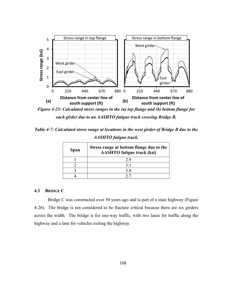
108

Figure 4-25: Calculated stress ranges in the (a) top flange and (b) bottom flange for

each girder due to an AASHTO fatigue truck crossing Bridge B.

Table 4-7: Calculated stress range at locations in the west girder of Bridge B due to the


Span Stress range at bottom flange due to the

AASHTO fatigue truck (ksi)

1 2.9 2 3.1 3 3.8 4 2.7

4.3 BRIDGE C

Bridge C was constructed over 50 years ago and is part of a state highway (Figure

4-26). The bridge is not considered to be fracture critical because there are six girders

across the width. The bridge is for one-way traffic, with two lanes for traffic along the

highway and a lane for vehicles exiting the highway.


0

1

2

3

4

5St

ress

ran

ge (

ksi)


880 210 6704400 880

Stress range in bottom flange

East girder

West girder

(a) (b)

210 6704400

Stress range in top flange

West girder

East girder

109

Figure 4-26: Bridge C.

4.3.1 Geometry

Bridge C has a length of 210 ft, featuring spans lengths of 35 ft, 47.5 ft, 35 ft, 57.5

ft, and 35 ft. The five-span continuous bridge is non-composite and has skewed supports

(20°40′) due to traffic beneath the bridge. The span distances shown in Figure 4-27 are

measured along the centerline of the bridge. Traffic travels in only one direction (west to

east) at the three-lane bridge (two lanes are highway and one lane is for an exit ramp).

Figure 4-27: Plan view of Bridge C (cross frames are not shown).

The typical cross section for the bridge is shown in Figure 4-28. The total width

of the bridge is 49.5 ft, with three lanes that are 12-ft wide and sidewalks on each side of

the bridge. The longitudinal girders are rolled sections (W27x102) that are spaced 8′-4″

35′-0″Span 1

47′-6″Span 2

35′-0″Span 3

57′-6″Span 4

35′-0″Span 5

Girder 6

Girder 5

Girder 4

Girder 1Girder 2

Girder 3

NorthDirection of traffic

110

apart. Cross frames are spaced 16′-3″ on center to provide lateral stability. Cover plates

were added near the interior supports to increase the section modulus.

Figure 4-28: Bridge cross section and location of lane at Bridge C (looking east).


A total of thirty-two strain gages were installed on three girders at three locations

along the length of the bridge (Figure 4-30). The WSN (Section 4.5.2) data acquisition

system was used at this bridge. Gages were installed within 1″ of the exterior edge of

each side of the flange (Figure 4-29).

Figure 4-29: Strain gages installed within 1″ of the exterior edge of the flange.

The structural connections of interest at this bridge from a fatigue perspective are

the flange-flange welds (cover plates) and transverse stiffeners. The flange-flange welds

and transverse stiffeners are respectively classified as Category B and Category Cʹ by the

AASHTO LRFD Specifications (2010). As such, the transverse stiffener is the critical

fatigue detail for where the strain gages are attached to the longitudinal girders. Because

5 spa. @ 8′-4″3′-4″ 4′-6″

3′-6″

1′-0″

6′-0″

1′-0″

12′-0″(left lane)

Girder 1

North South

Girder 2 Girder 3 Girder 4 Girder 5 Girder 6

12′-0″(right lane)

12′-0″(exit lane)

2′-0″W27x102, typ.

111

of the details used for the ends of the cover plates, those details are classified as Category

E′. However, no strain gages were installed near the ends of the cover plates.

Figure 4-30: Gage locations at Bridge C.

The nomenclature used to identify the gages is Location - Girder - Flange. So,

L1-3-BN is a gage installed at location 1 along girder 3 on the north side of the bottom

flange. The gage locations are summarized in Table 4-8.

Table 4-8: Summary of strain gages installed at Bridge C

Location Girder Number of gages

Description

1 1 4 Each side of the top and bottom flanges 1 3 4 Each side of the top and bottom flanges 1 5 2 Each side of the top flange 2 1 4 Each side of the top and bottom flanges 2 3 4 Each side of the top and bottom flanges 2 5 2 Each side of the top flange 3 1 4 Each side of the top and bottom flanges 3 3 4 Each side of the top and bottom flanges 3 5 4 Each side of the top and bottom flanges

4.3.3 Calculated Fatigue Response of Bridge C

One of the longitudinal girders was modeled as a line girder using SAP2000 (v

15) to calculate the response of the standard AASHTO fatigue truck (Figure 2-16). From

the moment envelope, the stress range from the fatigue truck can be calculated using

Equation 4-1. The increase in static loads due to dynamic effects ( ) was assumed to be

15% for the bridge per the AASHTO LRFD Specifications (2010). For bridges with

25′-0″Loc. 1

Girder 6

Girder 5

Girder 4

Girder 1Girder 2

Girder 3

17′-6″Loc. 2

20′-0″Loc. 3North

112

more than three girders, the live load distribution factor can be calculated using either the

lever rule or the empirical equations in the AASHTO LRFD Specifications (2010). The

live load distribution factors are summarized in Table 4-9 for cases in which the lever

rule is used for the trucks positioned in the center of the lanes identified in Figure 4-28.

When the lever rule is used, the method assumes that the entire load is supported by three

girders.

Table 4-9: Live load distribution factors for Bridge C based on lever rule.


Left lane Right lane Exit lane 1 0.1 - - 2 0.64 - - 3 0.26 0.4 - 4 - 0.6 0.16 5 - 0 0.64 6 - - 0.2

AASHTO Table 4.6.2.2.2b-1 in the LRFD Specifications can be used to calculate

the live load distribution factor ( ) for interior girders for bridges with multiple

girders. If this method is used, the distribution between all of the girders is not known,

instead only the maximum distribution factor for a single girder is calculated. The

distribution factor can be used for all of the interior girders because the load is assumed

to be transferred efficiently amongst multiple girders. Because traffic lanes can be

moved with time and vehicles are not always in the center of the lane, the distribution

factor does not depend on the location of the lane. The appropriate equation for steel

girders with a concrete bridge deck is presented below (Equation 4-3). The equation in

the AASHTO LRFD Specifications assumes a multiple presence factor of 1.2. In fatigue,

the presence of a single truck is desired, which is why the factor was removed below.

The parameters of the equation are within the range of applicability listed in the

AASHTO LRFD Specifications (2010).

113

11.2

0.0614

. .

12

.

Equation 4-3

where

distancebetweenlongitudinalgirders ft

length of span (ft)

thicknessofconcretedeck in.

(in.4)

modulusofelasticityofsteelbeam ksi

modulusofelasticityofconcretedeck ksi

momentofinertiaofsteelbeam non‐composite in.4

areaofsteelbeam non‐composite in.2

eccentricitybetweencentroidofbeamandconcretedeck in.

When the Guide Specification for Fatigue Evaluation of Existing Steel Structures

(AASHTO 1990) was developed, a different method for calculating the distribution factor

( ) was used for bridges with multiple girders (Equation 4-4).

3

Equation 4-4

empiricalfactorthatdependsonspanlength

The calculated distribution factors using both methods are summarized in Table

4-10. The distribution factors depend on the span length; thus, the values are different for

positive and negative moments. The values for each method ( and ) are

comparable for each location. Although, the difference between the lever rule

(maximum: 0.64) and (maximum: 0.471) is considerable. Between spans,

varies between 0.396 and 0.471. Because is used in the current specification, only

those values, along with the lever rule, were used in subsequent calculations in this

dissertation.

114

Table 4-10: Live load distribution factors for Bridge C based on AASHTO.

Span Distribution factor for interior girder

1 (positive moment) 0.471 0.463

1-2 (negative moment) 0.452 0.437





4 (positive moment) 0.396-0.403 0.419



The calculated moment envelope due to the passage of an AASHTO fatigue truck

is shown in Figure 4-31. Different sections in SAP2000 were used to represent the

different moment of inertias in the bridge due to the presence of cover plates. All

sections were symmetric and were modeled with a non-composite deck. All of the spans

experience both positive and negative moments. For a given gage location, the flexural

moment is positive when the truck is in the span with the gage, and negative when the

truck is in the adjacent span. The largest range in flexural moment (275 kip-ft) occurs in

the fourth span, near the middle of the span.


crossing a single girder at Bridge C.

-300

-200

-100

0

100

200

300

Mo

men

t (k

ip-f

t)

Distance from center line of west support (ft)

35 175117.582.50 210

275 kip-ft

+

Sign convention

-

115

If the distribution factors from the lever rule are used, the variation in stress range

for an AASHTO fatigue truck in the left, right, and exit lanes can be determined (Figure

4-32). The maximum calculated stress range from an AASHTO fatigue truck using the

lever rule is 9.2 ksi and occurs in the last span. If the distribution factor from the

AASHTO LRFD Specifications is used (Table 4-10), then the maximum stress range is

less (6.8 ksi).


for crossing Bridge C in the (a) left lane, (b) right lane, and (c) exit lane.

Using the calculated variation in stress range along the length of the bridge, the

stress range from an AASHTO fatigue truck can be estimated at the locations of the strain

gages. Table 4-11 summarizes the stress ranges for the three locations. The stress ranges

0

2

4

6

8

10

Stre

ss r

ange

(ks

i)



0

2

4

6

8

10

Stre

ss r

ange

(ks

i)


0

2

4

6

8

10

Stre

ss r

ange

(ks

i)


0

2

4

6

8

10

Stre

ss r

ange

(ks

i)



0

2

4

6

8

10

Stre

ss r

ange

(ks

i)


0 35 82.5 117.5 175 210

0 35 82.5 117.5 175 210

AASHTO fatigue truck in left lane and distribution factors from lever rule

0 35 82.5 117.5 175 210

(a) (b)

(c)

G2

G3 G1

G4

G3

G6

G5

G4

AASHTO fatigue truck in right lane and distribution factors from lever rule

AASHTO fatigue truck in exit lane and distribution factors from lever rule

116

listed are for distribution factors using the lever rule and the empirical equations. Girders

1 and 3 are not centered underneath the traffic lane, whereas Girder 5 is centered

underneath the traffic. As such, Girder 5 has a much higher expected stress range using

the lever rule as compared to Girders 1 and 3. The maximum stress range from a single

truck could be twice the magnitude of the values listed in Table 4-11 (AASHTO Manual

for Bridge Evaluation 2011).

Table 4-11: Calculated stress range at locations of Bridge C due to AASHTO fatigue

truck.

Location Maximum stress range due to AASHTO fatigue truck (ksi)

Girder 1† Girder 3† Girder 5† Interior* 1 1.0 (left) 2.7 (left), 4.6 (right) 7.4 (exit) 4.9 2 1.1 (left) 2.8 (left), 4.3 (right) 6.9 (exit) 4.6 3 1.4 (left) 3.7 (left), 5.7 (right) 9.2 (exit) 6.8

†Lever rule was used and fatigue truck is in the center of the lane listed in () *AASHTO LRFD (2010) was used to calculate the live load distribution factor.

4.4 BRIDGE D

Bridge D was constructed nearly 60 years ago and provides highway access

across a river (Figure 4-33). The bridge is not considered to be fracture critical because

there are seven girders across the bridge width. The bridge is for one-way traffic and

features four lanes for traffic along the highway.

Figure 4-33: Bridge D.

117

4.4.1 Geometry

Bridge D is a three-span, continuous, plate-girder bridge. The bridge is

symmetric about its centerline, with spans of 90 ft, 130 ft, and 90 ft (Figure 4-34).

Traffic travels along one direction (east to west) at the bridge. The thickness of the

flanges changes along the length to increase the section modulus over the interior

supports and in the middle of each span.

Figure 4-34: Plan view of Bridge D.

The typical cross section for the bridge is shown in Figure 4-35. The total width

of the bridge is 56.8 ft, with four, 12-ft traffic lanes. Each side of the bridge features

shoulders and sidewalks that are 2′-0″ and 2′-5″ wide, respectively. The plate girders are

64″ deep and spaced 8′-4″ apart. The flanges have a constant width of 16″ and a

thickness that varies at the interior pier and middle span for increased moment capacity.

The bridge is non-composite with cross frames that are spaced 22′-6″.

Figure 4-35: Cross section of Bridge D (looking west).

90′-0″ Span 1

130′-0″ Span 2

90′-0″ Span 3

Girder 1Girder 2

Girder 3Girder 4

Girder 5Girder 6


Girder 7

North

12′-0″(left lane)

2′-5″

South

2′-0″

6 spa. @ 8′-4″ 3′-5″

Girder 1

North3′-5″

Girder 2 Girder 3 Girder 4 Girder 5 Girder 6 Girder 7

2′-5″12′-0″(center-left lane)

12′-0″(center-right lane)

12′-0″(right lane)

2′-0″

118


A total of twenty-eight strain gages were installed on four girders at three

locations along the length of the bridge (Figure 4-36). Both the CompactRIO (Section

4.5.1) and WSN (Section 4.5.2) data acquisition systems were used at this bridge. Gages

were installed 4″ from the exterior edge of the flange. For Girder 3, gages were installed

4″ from each side of the flange.

Figure 4-36: Locations of gages at I-girder Bridge D.

The nomenclature used to identify the gages is Location - Girder - Flange. So,

L1-3-BN is a gage installed at location 1 along girder 3 on the north side of the bottom

flange. The gage locations are summarized in Table 4-12.

Table 4-12: Summary of strain gages installed at Bridge D

Location Girder Number of gages

Description

1 2 2 One gage on the top and bottom flanges 1 3 4 Each side of the top and bottom flanges 1 4 2 One gage on the top and bottom flanges 1 5 2 One gage on the top and bottom flanges 2 3 4 Each side of the top and bottom flanges 2 4 2 One gage on the top and bottom flanges 2 5 2 One gage on the top and bottom flanges 3 2 2 One gage on the top and bottom flanges 3 3 4 Each side of the top and bottom flanges 3 4 2 One gage on the top and bottom flanges 3 5 2 One gage on the top and bottom flanges

Based on where strain gages were installed on the longitudinal girders, the

structural connections of interest at this bridge from a fatigue perspective are the

54′-0″ Loc. 3

65′-0″ Loc. 1

20′-0″ Loc. 2

Girder 1Girder 2

Girder 3Girder 4

Girder 5Girder 6

Girder 7

North

119

transverse stiffeners, flange-flange welds (cover plates), and web-flange welds.

According to the AASHTO LRFD Specifications (2010), the transverse stiffeners are

characterized as Category C′ and the welds (flange-flange and web-flange) as Category

B. As such, the transverse stiffener is the critical fatigue detail for where the strain gages

are attached to the longitudinal girders. Because of the details used for the ends of the

cover plates, those details are classified as Category E′. However, no strain gages were

installed near the ends of the cover plates.

4.4.3 Calculated Fatigue Response of Bridge D

A line analysis of one of the longitudinal girders was performed using SAP2000

(v 15) to calculate the moment envelope from a standard AASHTO fatigue truck (Figure

2-16). The stress range can be calculated using Equation 4-1 and a dynamic impact

factor ( ) of 15%. The live load distribution factor can be computed from either the

lever rule or the AASHTO empirical equations (Equation 4-3 and Equation 4-4). The

center of each line identified in Figure 4-35 was used to calculate the distribution factors

using the lever rule (Table 4-13). The distribution factors from the empirical equations

are summarized in Table 4-14.

Table 4-13: Live load distribution factors for Bridge D based on lever rule.


Left lane Center-left

lane Center-right

lane Right lane

1 0.26 - - - 2 0. 64 - - - 3 0.1 0.04 - - 4 - 0.64 0.32 - 5 - 0.32 0.64 0.1 6 - - 0.04 0.64 7 - - - 0.26

120

Table 4-14: Live load distribution factors for Bridge D based on AASHTO.

Span Distribution factor for interior girder


1-2 (negative moment) 0.427 0.368 2 (positive moment) 0.400 0.362

2-3 (negative moment) 0.427 0.368 3 (positive moment) 0.429 0.379

The calculated moment envelope due to the passage of an AASHTO fatigue truck is

shown in Figure 4-37. Different sections in SAP2000 were used to represent the different

moment of inertias in the bridge due to the changes in values of the flange thickness.

Though, all sections were symmetric and were modeled with a non-composite deck. All

of the spans experience both positive and negative moments. For a given gage location,

the flexural moment is positive when the truck is in the span with the gage, and negative

when the truck is in the adjacent span. The largest range in flexural moment (1,000 kip-

ft) occurs in the center span, near the middle of the span.


crossing a single girder at Bridge D.

If the distribution factors from the lever rule are used, the variation in stress range

for an AASHTO fatigue truck in each lane can be computed (Figure 4-38). The

-900

-600

-300

0

300

600

900

Mo

men

t (k

ip-f

t)

Distance from center line of east support (ft)90 220

1,000 kip-ft

0 310

+

Sign convention

-

121

maximum calculated stress range from an AASHTO fatigue truck using the lever rule is

8.3 ksi and occurs in the end spans. If the distribution factor from AASHTO is used

(Table 4-14), then the maximum stress range is less (5.6 ksi).


for crossing Bridge D in the (a) left lane and (b) left-center lane.

Using the calculated variation in stress range along the length of the bridge

(Figure 4-38), the stress range from an AASHTO fatigue truck can be estimated at the

locations of the strain gages. The stress ranges for the three gage locations and different

distribution factors (lever rule and empirical equations) are summarized in Table 4-15.

Location 3 corresponds to the highest stress range for the gage locations. The maximum

stress range from a single truck could be twice the magnitude of the values listed in

Figure 4-38 (AASHTO Manual for Bridge Evaluation 2011).

Distance from center line of east support (ft)

0

2

4

6

8

10

Stre

ss r

ange

(ks

i)

Distance from center line of east support (ft)

AASHTO fatigue truck in left lane and distribution factors from lever rule

(a) (b)

G2

G3 G1

AASHTO fatigue truck in center-left lane and distribution factors from lever rule

G2

G3

G4

The shape of the curve for center-right lane will be similar to (b) and the curve for the right lane will be similar to (a)

122

Table 4-15: Calculated stress range at locations of Bridge D due to AASHTO fatigue

truck.

Location Maximum stress range due to AASHTO fatigue truck (ksi)

Girder 2† Girder 3† Girder 4† Girder 5† Interior*

1 6.6 (left) 6.6 (left-center)

3.3 (left-center)

5.5 (right-center) 4.1


2.0 (left-center)



4.0 (left-center)


†Lever rule was used and fatigue truck is in the center of the lane listed in () *AASHTO LRFD Specifications (2010) was used to calculate the live load distribution factor.

4.5 DATA ACQUISITION SYSTEM & SENSORS

Two types of data acquisition systems from National Instruments (NI) were used

to obtain dynamic strain data at the four bridge sites. The wired (CompactRIO) and

wireless (WSN) systems were used to determine the fatigue cycles from vehicles crossing

the bridge using the simplified rainflow algorithm, and the resulting distribution of stress

ranges were used to calculate the remaining fatigue life. Strain gages were the primary

type of sensor used at the bridge sites. Strains were converted to stresses using Hooke’s

Law and a modulus of elasticity for steel of 29,000 ksi.

4.5.1 Wired System - CompactRIO

The NI CompactRIO is a wired system that is capable of high-resolution,

configurable data acquisition and control. For the bridge sites, NI-9237 modules were

combined with the CompactRIO to acquire high-speed quarter-, half-, and full-bridge

measurements. Each module supports four channels and each channel has a separate, 24-

bit analog-to-digital converter (ADC). The module utilizes field-programmable gate

arrays (FPGA) to produce hardware-timed measurements that can be synchronized across

modules. Using the internal master timebase, the module supports sampling rates

123

between 1,613 Hz and 50,000 Hz. A 2.5-V excitation was used along with 350-Ω

quarter-bridge completion resistors.

Figure 4-39: CompactRIO data acquisition system with NI-9237 modules (wired).

4.5.1.1 Programming

With the onboard processor (533-800 MHz) and nonvolatile memory (2-4 GB),

each CompactRIO was programmed for data acquisition and analysis. Each program was

created in the LabVIEW Real-Time (RT) environment. To handle the fast data

acquisition, the FPGA captured hardware-timed data at 2,000 Hz and transferred the data

to the RT environment. In the RT environment, data were downsampled to 50 Hz and

processed using a custom simplified rainflow program. Due to the size of the processor

and memory, other programs can run simultaneously on the CompactRIO. As such, the

raw strain history was also saved at some bridges, while only events greater than a

specified threshold were saved at other bridges.

4.5.2 Wireless System - Wireless Sensor Networks (WSN)

The other data acquisition system employed at the bridge sites was the Wireless

Sensor Network (WSN) platform from NI (Figure 4-40). With such a wireless system,

sensors are connected to nodes that acquire data and send the data wirelessly to a

gateway/computer where it can be stored temporarily or permanently. The gateway

creates the wireless network that enables the nodes to transmit data. The WSN platform

utilizes a narrow-band protocol (IEEE 802.15.4) to transmit data. The protocol is well-

suited for bridge deployments because it is lower power than other broader-bandwidth

protocols (IEEE 802.11). In addition, narrow-bandwidth protocols performed better

124

(longer distances and more consistent communication links) in steel-bridge environments

due to the presence of multi-path effects (Fasl, et al. 2012b).

Figure 4-40: Wireless strain node data acquisition system (WSN-3214).

A specialized gateway, which is connected to a computer or a controller, is

required to create the wireless network. Nodes connect to the gateway and send data

across the network as either mesh routers (always awake) or end nodes (only awake when

scanning and sending data). Because mesh routers are always on, they are not considered

to be low-power devices. However, the mesh routers offer a powerful capability to the

network. Mesh routers increase the redundancy of the network and increase the area that

can be monitored because they can transfer data from end nodes or other routers back to

the gateway (Figure 4-41).

Figure 4-41: Typical network configuration for bridges.

The wireless strain node, WSN-3214, is capable of capturing dynamic data from

four analog channels. A variety of sensors can be used, including quarter-bridge (built-in

350-Ω and 1,000-Ω completion resisters), half-bridge, and full-bridge inputs with a 2.0-V

Gateway

Router

End Nodes

125

bridge excitation. The embedded, Texas Instrument MSP430 microprocessor has the

ability to run LabVIEW WSN graphical programs, thereby enabling onboard data

processing at the node. Using LabVIEW WSN, the strain node can be easily customized

for a particular application. The node also features built-in shunt calibration and remote

sensing to reduce lead-wire errors and 2-MB onboard memory buffers for data storage.

Four internal AA batteries or an external DC power source, such as an energy harvester,

can be used to power the node.

The strain node minimizes electrical noise while maintaining low-power

consumption through a robust ADC design. Because low noise often means more power

and low power often means more noise, a configurable ADC was chosen for the strain

node. Successive-approximate (SAR) converters and delta-sigma converters are the two

most commonly-used ADC in data acquisition applications. SAR converters work well

in multiplexed systems, whereas delta-sigma converters provide high resolution through

oversampling and digitally filtering the analog signal. To deliver the optimum

combination of resolution, low-noise performance, speed, and low-power operation, the

node utilizes a multiplexed, oversampled SAR ADC with digital filtering performed by

an onboard FPGA (fully programmable gate array). The FPGA also enables fast

sampling (1 to 2,000 Hz) without overwhelming the microprocessor. The result is

measurements that are hardware-timed with 20-bit ADC resolution. To balance the

tradeoffs of noise filtering, power consumption, and speed, the user can choose the

measurement time (aperture time) or one of the 50-Hz/60-Hz filtering options.

4.5.2.1 Programming

With a wireless system, data transfer is a primary concern, especially in low-

bandwidth systems. Often, the most power-hungry component in a wireless node is the

radio (Lynch, et al. 2004). By performing a custom analysis with the microprocessor of

each node and only sending the analysis results, the amount of data transmitted can be

reduced. As such, power is saved while not overwhelming the limited bandwidth of the

IEEE 802.15.4 protocol.

126

The impact to the bandwidth of the wireless network from performing an analysis

on the node as compared to the gateway can be imagined by considering the example of a

rainflow analysis. The node might be configured to acquire data at 50 samples per

second to capture the dynamic effects of trucks crossing the bridge. In a 30-minute

period, over 90,000 samples per channel (360,000 samples per node) would need to be

sent over the air if the gateway were to perform the analysis. Assuming no loss of data

and maximum efficiency of the network, approximately ten nodes would cause the

bandwidth of the IEEE 802.15.4 network to be exceeded. As the efficiency of the

network decreased and loss of data occurred, the number of nodes allowed on the

network would also decrease. In contrast, by embedding the program on the node and

performing the analysis in real-time, the number of data points sent over the air could be

reduced to the results of the analysis (a couple hundred samples per channel in a 30-

minute period). Because the engineer or bridge owner can use the results directly, no

information is lost by sending only the results of the analysis, and there would still be

some bandwidth to transmit triggered strain histories (only data above a threshold).

A custom program was developed to allow each strain node to be configured over

the air and operate in a variety of modes of operation. By creating string messages that

are sent by the gateway over the air to the node, a user can configure the scan period,

sampling rate, number of samples, aperture time, channel configuration (quarter bridge,

half bridge, and full bridge), gage factor, and parameters related to the rainflow analysis.

A sub-program was added to the node that can parse the string into configuration

parameters. Thus, the node can be configured for a slow sampling rate for non-critical

times and switched to a faster scan rate when dynamic data are desired. The custom

program has five distinct modes of operation for the node, depending on the application

need: no data, streaming data (data sent back each scan period), triggered data, rainflow

analysis (for counting the number and amplitude of fatigue cycles), and rainflow analysis

plus triggered data. The rainflow algorithm is based on the method described in

Downing and Socie (1982).

127

When multiple nodes are connected to a single gateway, configuring all of the

channels for the rainflow parameters and scan properties can be challenging. A

LabVIEW program was created to automate the process of updating all of the nodes. The

user must first create a configuration file. The configuration file has to be formatted in a

specific manner; thus, a LabVIEW VI was developed to assist with creation of the

configuration file (nodes connected to the gateway are auto-detected to make

configuration easier). The configuration file must then be uploaded to the gateway

through a program that detects all of the nodes, sends the configuration file to each

individual node as string messages, receives confirmation that each node has been

configured, and then starts the desired program on the node (no data, streaming, trigger

data, rainflow, or rainflow and trigger data). The gateway also uses the configuration file

to determine programmatically which node channels to access in the LabVIEW Real-

Time environment so that it can be saved.

4.5.3 Sensors

Two types of sensors were used at the four bridges: strain gages and crack

propagation gages. For Bridges A-C, the CEA-06-250UN-350/P2 strain gage from

Vishay Micromeasurement was used. The general-purpose, foil strain gage is

temperature compensated for mild carbon steel and has three lead wires. The gages are

0.250-in. long with a resistance of 350 Ω. For the wired data acquisition systems, the

gage wires were spliced to a thicker, insulated wire to minimize possible electrical

interference. For the wireless systems, no additional wire was needed as the wireless

node could be placed next to the strain gages. At Bridge D, sealed, weldable strain gages

were used. The weldable gages were from Hitech Products, Inc. Crack propagation

gages from Vishay Micromeasurement (TK-09-CPA02-005/DP) were installed at Bridge

A due to the presence of active cracks.

The sensors were installed to the steel and moisture-protected following

manufacturer recommendations. All of the foil gages (strain and crack propagation) were

applied to the steel girders using the CN adhesive from Texas Measurement. For

128

moisture protection, a two-part scheme was used. A crystalline wax and then a silicone

were applied to the region surrounding and including the gage. The weldable gages were

installed to the steel by adding spot welds around the surface of the gage. Rubber tape

and foil tape were applied over the gage to protect it from moisture. Samaras (2013)

provides a detail discussion on the application and protection techniques for strain gages.

4.6 SUMMARY

Four steel bridges were investigated to characterize the fatigue response of critical

connections due to vehicles crossing each bridge. The instrumentation locations were

identified in this chapter, as were the critical details corresponding to the locations of the

strain gages. At each bridge, a fatigue analysis was conducted, which consisted of a line-

girder analysis and calculating the moment envelope due to the AASHTO fatigue truck,

to determine the locations with the largest stress ranges. The results of the structural

analyses will be used in Chapter 7 to estimate the remaining fatigue life.

The data acquisition equipment used at each bridge are also summarized in

Section 4.5. Both wired (CompactRIO) and wireless systems were utilized at the bridges,

along with two types of sensors (strain gages and crack propagation gages).

129

CHAPTER 5

Interpretation of Measured Fatigue Response

of Four Bridges

Strain gages were installed at four bridges to determine the current distribution of

stress ranges from daily traffic and calculate the accumulation of fatigue damage during

the monitoring period. Descriptions of the four bridges are presented in Chapter 4, as are

the locations of the strain gages. Dynamic strain histories were obtained at an effective

scan rate of 50 Hz at all of the bridges and processed using the simplified rainflow

algorithm (Section 3.1). In general, only the results of the rainflow analysis were

archived, expect during a live load test that occurred at Bridge A, in which strain histories

induced by a test vehicle were recorded. The results of that load test are discussed in

Chapter 6.

The average extent of fatigue damage induced by vehicles crossing the bridge was

characterized using the index stress range (Section 3.2.2). In some situations, the

effective stress range was also calculated (Section 3.2.1); however, only the index stress

range was used to make comparisons between gages and/or bridges discussed in this

chapter. The spectra of stress ranges were verified using the visualization techniques

described in Chapter 3 (contribution to damage (Section 3.3.1) and cumulative damage

(Section 3.3.2)). The amount of fatigue damage determined from the field investigations

were used to calculate the remaining fatigue life of the bridges as presented in Chapter 7.

Data from only a few gages for each bridge are presented in this chapter, but summary

data from all gages are presented in the appendices.

As discussed in Section 3.1, the strain histories were processed by the simplified

rainflow algorithm in 30-minute segments. The bins were summed in various ways to

evaluate the variation in fatigue damage as a function of time of day and day of the week.

With the CompactRIO system (Section 4.5.1) at Bridge A, the 30-min periods were

synchronized on the half hour (1:00 AM, 1:30 AM, etc.) and thus were easy to combine.

130

In contrast, the 30-min periods recorded using the WSN systems (Section 4.5.2) (Bridges

B, C, and D) began when the wireless node started sampling data and were not oriented

on the half hour. As such, to group those acquisition periods, any period that started

between 12:15 AM and 12:45 AM was oriented at 12:30 AM and so forth.

The monitoring periods for each bridge are defined in Section 5.1. Based on

measured data from those monitoring periods, the fatigue damage was evaluated for each

bridge in Section 5.2. The variation in fatigue damage at Bridges A, B, and C are

summarized in Section 5.3.

The construction of the retrofit at Bridge A was tracked using the index stress

range concept (Section 5.4). Using the index stress range, the different phases of the

construction could easily be identified and the benefit of the retrofit quantified.

5.1 DURATION OF MONITORING

Bridges A and B were monitored the longest because both bridges were

considered to be fracture critical and those bridge types were the intended target of the

research project. Whereas the measured fatigue response was tracked for over a year at

Bridge A and multiple months at Bridge B, Bridges C and D were only monitored for

time periods ranging from a few days to a few weeks.

Powering the data acquisition system at each bridge was a concern and impacted

how much data were collected. Because longer monitoring periods were envisioned at

Bridges A and B, solar panels were installed to power the equipment. The goals of

monitoring Bridges C and D were to validate the wireless data acquisition equipment

(Section 4.5.2). As such, both bridges were monitored for a shorter period, and batteries

were used to power the WSN data acquisition systems.

The first iteration of the solar panel (85 W) at Bridge A was too small to power

the system during the winter months and numerous interruptions in the data acquisition

occurred. A larger solar panel (130 W) was installed at the site in August 2011 (Figure

5-1(a)), along with a maximum power point tracking (MPPT) charge controller, which

greatly improved performance. Since August 2011, the system was continuously online

131

with minimal downtown. There were a few instances during prolonged periods of rain

when data were not captured due to inadequate solar exposure. For instance, rainy

conditions prevailed in seventeen of the thirty-one days of December 2011, which caused

loss of data for most of the month.

An 85-W panel was connected to the concrete barrier of Bridge B using post-

installed anchors (Figure 5-1(b)). The panel was not expected to be a long-term solution

for the bridge, but was large enough for data acquisition during spring and summer

months.

Figure 5-1: Solar panels installed at (a) Bridge A and (b) Bridge B.

5.1.1 Bridge A

Monitoring at Bridge A began in March 2011 and continued until August 2012.

Within the first few months, the following key observations were made: (1) some large

stress ranges (greater than 15 ksi) were measured by many of the gages installed along

the top flange of the east longitudinal girder and (2) a few of the cracks identified during

the hands-on inspections were growing. The large stress ranges were alarming from a

fatigue perspective because the fatigue life depends on the cube of the stress range.

A crack propagation gage was installed at the tip of a crack in the welded

connection between the top flange of the east girder and the top flange of floor beam 34.

This crack was identified during the hands-on inspection conducted by the bridge owner

132

in fall 2010. The gage features twenty wires distributed over a width of 0.4″. The wires

of the gage fracture due to growth of the crack, which changes the resistance of the gage.

By measuring the resistance, the crack length can be monitored. Due to the step-wise

nature of the gage, the change in resistance is fairly small (0.2-0.5 Ω) when only a few

wires have broken. However, after the majority of the wires have broken, the change in

resistance due to a wire break is greater than 10 Ω. With the CompactRIO data

acquisition system and measuring the resistance every 30 min, the drift of the gage due to

temperature was less than the change due to a wire break.

The response of the crack propagation gage near floor beam 34 is presented in

Figure 5-2 for a 28-day period in spring 2011. Eleven wires of the crack propagation

gage broke during that period, with a wire breaking approximately every three days. As

such, the crack growth was approximately 0.007″ per day during that period.

Figure 5-2: Crack growth at floor beam 34 in east longitudinal girder during 28-day

period.

Because the crack continued to grow in the flange of the east longitudinal girder

at the location of the welded connection to floor beam 34 over the next 1.5 months at

nearly the same rate, the fatigue life can be assumed to have been exceeded in 2011.

Based on continuous growth of cracks in critical regions of Bridge A, the bridge owner

decided to construct a replacement bridge and remove this structure from service.

However, because it will take 2-3 years to replace the bridge, a retrofit plan was

0

3

6

9

12

15

18

05/02 05/07 05/12 05/17 05/22 05/27 06/01

Res

ista

nce

(o

hm

s)

Time

11 wire breaks | Crack growth of 11x0.02″ = 0.22″ (28 days)

Assumed

Res

ista

nce

(Ω

)

133

developed to maintain the load-carrying capacity of the bridge until the replacement was

designed and constructed.

The chosen retrofit is discussed in Section 4.1.3. The fatigue response of Bridge

A was drastically different before and after the construction of the retrofit. As is

discussed in Section 5.4, the retrofit significantly reduced the fatigue damage induced in

the top flanges of the longitudinal girders at floor beams 34 and 35. For gage locations

on the bottom flange, the rate of change in the fatigue damage decreased, but not nearly

as much as the top flanges. Because the accumulation of fatigue damage in the top flange

was nearly zero and much larger in the bottom flange, the behavior is representative of

composite action between the concrete deck and steel longitudinal girder.

Due to the changes in fatigue behavior of the bridge, the monitoring periods were

broken into different phases. The first phase occurred before the construction of the

retrofit and lasted from March 2011 to August 2011. Due to power issues, a total of 71

full days of data were obtained during this phase. The fatigue damage was characterized

based on the data recorded during those 71 days and used to calculate the remaining

fatigue life in Chapter 7. Only full days (24 hours in a single day) were considered in the

analysis. Partial days were neglected from the analysis because the traffic patterns varied

significantly with the time of day (Section 5.3.1). The distribution of the full days among

the days of the week is summarized in Table 5-1. As is subsequently discussed, the

amount of fatigue damage depended on the day of the week. Therefore, if the estimate of

fatigue damage is based on a non-uniform distribution of days, there is the possibility that

the estimate will be skewed. The data before the construction of the retrofit (Table 5-1)

were used to evaluate the skew in the estimate.

Construction of the retrofit took place from August 2011 to November 2011. The

characterization of fatigue damage was not as interesting during the construction of the

retrofit because a new detail was assumed once the construction was finished. After the

retrofit was finished, the bridge was monitored from November 2011 to August 2012, in

which over 180 days of data were collected (Table 5-2). For this phase, the distribution

134

of days was fairly uniform. The fatigue damage for that period was determined to

evaluate the benefit of the retrofit.

The response of two gages will be discussed in this chapter while the responses of

all gages are summarized in Appendix A & Appendix B.

Table 5-1: Distribution of full days of rainflow data before retrofit at Bridge A.

Day of the week Number of full days Monday 9 Tuesday 8

Wednesday 12 Thursday 10

Friday 10 Saturday 13 Sunday 9

Total 71

Table 5-2: Distribution of full days of rainflow data after construction of the retrofit at

Bridge A.

Day of the week Number of full days Monday 25 Tuesday 28

Wednesday 27 Thursday 24

Friday 27 Saturday 28 Sunday 27

Total 186

5.1.2 Bridge B

The fatigue behavior of Bridge B was tracked for nearly four months. Both

CompactRIO and WSN data acquisition systems were utilized at this bridge. One of the

strain gages from the CompactRIO system will be discussed in Section 5.2, and two

strain gages connected to the WSN system will be discussed in Section 5.2.3. Initially, in

135

April 2012, only two wireless nodes were installed at the bridge, one node in the first

span and one node in the second span. Two months later, June 2012, several WSN

routers were added to the bridge to expand the network to feature a node in each of the

spans. A router in each span was required to wirelessly transmit data from gages located

in Span 4 to the gateway in Span 1. The wireless system proved beneficial at this bridge

because thousands of feet of cable would have been needed if a CompactRIO would have

been used for all of the gage locations. The responses of two gages are discussed in this

chapter while the responses of all gages are summarized in Appendix C.

When evaluating the fatigue damage during the monitoring period, only full days

were considered. The distribution of those days is summarized in Table 5-3. As seen

from the table, the days were fairly evenly distributed.

Table 5-3: Distribution of full days of rainflow data at Bridge B.

Day of the week Number of full days Span 1 Span 3

Monday 10 5 Tuesday 9 5

Wednesday 9 4 Thursday 9 4

Friday 11 4 Saturday 10 5 Sunday 10 4

Total 68 31

5.1.3 Bridge C

Bridge C was monitored for approximately one month. Because batteries were

used at the site to power the WSN data acquisition system, data were not collected

continuously. As such, long-term estimates of the remaining fatigue life were not made

from the data at this bridge because so few full days of data were collected. Because nine

wireless nodes were needed for the instrumentation, one of the nodes was configured as a

136

router while the other eight could be end nodes. The results of all of the WSN gages are

summarized in Appendix D.

5.1.4 Bridge D

Bridge D was monitored for less than one week. Long-term estimates of the

remaining fatigue life were not made from the data at this bridge because so few full days

of data were collected. However, the techniques described in Chapter 3 can be applied to

the data set. Both CompactRIO and WSN data acquisition systems were utilized at this

bridge. Data from the CompactRIO system were discussed in Section 3.4, whereas data

from two of the gages on the WSN system are discussed in this chapter. The responses of

all of the WSN gages are summarized in Appendix E.

5.2 MEASURED FATIGUE RESPONSE DURING MONITORING PERIOD

Two strain gages from each bridge are presented in this section to calculate the

measured fatigue responses during the monitoring periods. For Bridge A, data are

presented for the monitoring periods before and after the retrofit. The index stress range

was used to make comparisons between the bridges. For Bridge A, an index stress range

of 4.5 ksi was used because the critical fatigue detail for this bridge was Category E, and

4.5 ksi corresponds to the CAFL for this detail category. Transverse stiffeners (Category

C′) were the critical fatigue details for the other three bridges, which corresponds to a

CAFL of 12 ksi. Therefore an index stress range of 12 ksi was used at Bridges B, C, and

D.

As discussed in Chapter 3, electromechanical noise produces fictitious stress

fluctuations that do not induce fatigue damage and should be truncated from a fatigue

analysis. The electromechanical noise of each data acquisition system was determined in

the laboratory. For the CompactRIO, it was approximately 1 microstain and 2-3

microstrain for the WSN system. As such, the minimum amplitude of the rainflow

analysis was set at 2 microstrain for the CompactRIO and 5 microstrain for the WSN

system; cycles less than the minimum amplitude were identified, but not included in the

137

rainflow data. As a reference, a 1 microstrain strain change corresponds to a stress

change of approximately 0.03 ksi.

The electromechanical noise at a particular bridge can be higher than these typical

values because the concentration of steel and power lines at each site can affect the noise.

To validate the levels of electromechanical noise at some of the bridges, strain gages

were attached to plates that were not connected to the bridge. The plates were able to

expand and contract freely; thus, any cycles that were identified by the rainflow

algorithm for the gages attached to these plates were considered to be caused by

electromechanical noise and/or temperature drift. The WSN nodes with external batteries

at Bridges B and C were susceptible to higher levels of electromechanical noise

(approximately 15-20 microstrain) because the nodes were not grounded properly.

The electromechanical noise was determined at Bridge B by evaluating the cycles

in the rainflow bins for the plates that were not attached to the bridge. Two gages were

installed next to each other on the bottom flange of the longitudinal girder in Span 1 at

Bridge B, with one gage connected to the CompactRIO data acquisition system and one

gage connected to the WSN system (Figure 5-3). The contribution of each rainflow bin

to the fatigue damage ( , 12 ) was similar for both systems for stress ranges above

0.4 ksi. However, the two systems diverge at stress ranges below 0.4 ksi, with the

rainflow bins from the WSN system contributing significantly more than the rainflow

bins from the CompactRIO system. The response of a strain gage attached to one of the

plates that was not attached to the bridge is also presented in Figure 5-3. As can be seen,

stress ranges below 0.4 ksi contribute significantly to the damage, at a similar scale as the

longitudinal-girder gage connected to the WSN system. Because stress cycles were

measured in a plate with no load applied (free to expand and contract), the cycles are due

to fluctuations in the data acquisition system from electromechanical noise. Therefore,

cycles less than 0.4 ksi were truncated from the WSN nodes at Bridge B.

At Bridge C, both internal-AA and external batteries were used to power the

WSN nodes. For the nodes with internal batteries, the contribution of the lower bins was

138

minimal, whereas the contribution of the lower bins was significant for the nodes with

external batteries (Section 5.2.4). One of the nodes powered by internal-AA batteries

was used for the gages attached to the plate. With that node, no cycles were identified by

the rainflow algorithm. Therefore, the minimum amplitude was set high enough for the

WSN nodes powered by internal-AA batteries. For the node powered by the external

battery, cycles less than 0.4 ksi should be truncated from the rainflow analysis due to

electromechanical noise.

Figure 5-3: Contribution of each bin to , at Bridge B for gages connected

to the CompactRIO and WSN data acquisition systems.

Based in part on the experiences of the research team at Bridges B and C, the

WSN-3214 user guide (National Instruments 2012) provides a method for properly

grounding the external battery and strain gages to the node to minimize the

electromechanical noise.

For each bridge, the rainflow bins had a width of 5 microstrain (0.145 ksi). Based

on the results of the structural analysis discussed in Chapter 4, Bridge A had the largest

expected stress ranges from the crossing of an AASHTO fatigue truck. As such, at

Bridge A, at total of 200 rainflow bins were used, which allowed a maximum stress range

of 29 ksi to be identified and sorted into one of the bins. At the other three bridges, only

100 rainflow bins were used, which corresponds to a maximum stress range of 14.5 ksi.

0.0

0.2

0.4

0.6

0.8

1.0


Co

ntr

ibu

tio

n t

o

WSN system (longitudinal girder)

cRIO system (longitudinal girder)

WSN system (plate not attached to girder)

139

5.2.1 Bridge A (Before construction of the retrofit)

The total accumulation of fatigue damage estimated from field monitoring can be

determined from the histogram of stress ranges using either the effective stress range or

index stress range. Two gages are discussed in this section, one attached to the west

girder and one attached to the east girder. As a reminder of the nomenclature outlined in

Chapter 4, Gage W-34s-TE was installed on the east side of the top flange of the west

longitudinal girder near the connection to floor beam 34, whereas gage E-34s-TW was

installed on the west side of the top flange of the east longitudinal girder near the

connection to floor beam 34. In this section, W-34s-TE and E-34s-TW are referred to as

the gages on the east and west girders, respectively.

Figure 5-4: Histogram of stress ranges before construction of the retrofit (average of

71 days) for gages attached to the top flange of the (a) west girder and (b) east girder.

The histogram of average number of cycles in a day recorded by each gage is

presented in Figure 5-4. The maximum measured stress ranges were 17.2 ksi and 24.9

ksi for the gages installed on the west and east girders, respectively. Some strain

histories were captured at Bridge A before the construction of the retrofit and verified

that the larger stress ranges were induced from trucks crossing the bridge. The fatigue

damage was calculated using both the effective stress range ( , and ) and the index

0.001

0.01

0.1

1

10

100

1000

10000

100000

0 10 20 30

Ave

rage

nu

mb

er o

f cy

cle

s p

er d

ay

Stress range (ksi)

0.001

0.01

0.1

1

10

100

1000

10000

100000

0 10 20 30

Ave

rage

nu

mb

er o

f cy

cle

s p

er d

ay

Stress range (ksi)(a) (b)

38,000

17.2 ksi

41,400

24.9 ksi

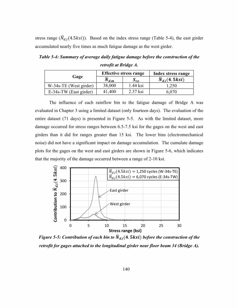
140

stress range ( , 4.5 ). Based on the index stress range (Table 5-4), the east girder

accumulated nearly five times as much fatigue damage as the west girder.

Table 5-4: Summary of average daily fatigue damage before the construction of the

retrofit at Bridge A.

Gage Effective stress range Index stress range

, , . W-34s-TE (West girder) 38,000 1.44 ksi 1,250 E-34s-TW (East girder) 41,400 2.37 ksi 6,070

The influence of each rainflow bin to the fatigue damage of Bridge A was

evaluated in Chapter 3 using a limited dataset (only fourteen days). The evaluation of the

entire dataset (71 days) is presented in Figure 5-5. As with the limited dataset, more

damage occurred for stress ranges between 6.5-7.5 ksi for the gages on the west and east

girders than it did for ranges greater than 15 ksi. The lower bins (electromechanical

noise) did not have a significant impact on damage accumulation. The cumulate damage

plots for the gages on the west and east girders are shown in Figure 5-6, which indicates

that the majority of the damage occurred between a range of 2-10 ksi.

Figure 5-5: Contribution of each bin to , . before the construction of the

retrofit for gages attached to the longitudinal girder near floor beam 34 (Bridge A).

0

100

200

300

400

0 5 10 15 20 25 30Stress range (ksi)

Co

ntr

ibu

tio

n t

o East girder

West girder

1,250 cycles (W-34s-TE)

6,070 cycles (E-34s-TW)

141

Figure 5-6: The cumulative fatigue damage before the construction of the retrofit for

gage attached to the (a) west girder and (b) east girder.

5.2.2 Bridge A (After the construction of the retrofit)

The same two gages discussed for before the construction of the retrofit are

discussed for the period after the cracked connections had been retrofitted. The gages are

located on the top flanges of the west and east longitudinal girders near the connections

to floor beam 34. For the remainder of this section, W-34s-TE is referred to as the gage

on the west girder, whereas E-34s-TW is referred to as the gage on the east girder.

The average daily cycles of stress ranges from November 2011 to April 2012 are

presented in Figure 5-7. The effective stress range and index stress range were calculated

for each distribution of stress ranges (Table 5-5). The maximum stress ranges were 29.1

ksi and 10.2 ksi for the gages on the west and east girders, respectively. As will be

discussed, the larger stress ranges in the west girder were not believed to be load induced,

but were due to spikes in the data acquisition system. However, the raw stress histories

from the large events at Bridge A were not saved and the responses of the gages could

not be verified. Validating these larger stress cycles highlights the need for an additional

program (besides the rainflow algorithm) on the data acquisition systems that can save

the stress histories from large events (seconds of data). As such, a triggering program

was developed for the data acquisition systems at the other three bridges.

0 10 20 30Stress range (ksi)

0

0.2

0.4

0.6

0.8

1

0 10 20 30

Ave

rage

dai

ly

cum

ula

tive

dam

age


1.2 ksi

9.4 ksi 17.2 ksi 24.9 ksi

2.7 ksi

10.8 ksi

95% of damage

2.5% of damage

95% of damage

2.5% of damage

142

Figure 5-7: Histogram of stress ranges after the construction of the retrofit (average of

94 days) for gages attached to the top flange of the (a) west girder and (b) east girder.

Table 5-5: Summary of average daily fatigue damage after the construction of the



, , . W-34s-TE (West girder) 121,000 0.48 ksi 150 E-34s-TW (East girder) 83,700 1.02 ksi 980

The contribution of each rainflow bin to the fatigue damage was evaluated (Figure

5-8). The damage in the east girder was larger than in the west girder. For the east

girder, the most damage occurred for stress ranges between 2-4 ksi, which is much

smaller than the response (6.5-7.5 ksi) at that location before the retrofit of the connection

detail (Figure 5-5). The measured stress ranges above 5 ksi did not have a significant

impact on the damage accumulation at that particular gage location, which reinforces the

idea that some composite action was gained in the retrofit. For the west girder, the most

damage occurred for stress ranges between 2-3 ksi. However, the larger stress ranges

(greater than 25 ksi) did have an influence on the total amount of damage.

0.001

0.01

0.1

1

10

100

1000

10000

100000

0 10 20 30

Ave

rage

nu

mb

er o

f cy

cles

per

day

Stress range (ksi)

0.001

0.01

0.1

1

10

100

1000

10000

100000

0 10 20 30

Ave

rage

nu

mb

er o

f cy

cles

per

day


121,000

29.1 ksi

83,700

10.2 ksi

143

Figure 5-8: Contribution of each bin to , . during the monitoring period

after the construction of the retrofit for gages on the west and east girders.

Considering the cumulative damage graphs for both gages (Figure 5-9), the

majority of the damage occurred over a rather large range (0.2-29 ksi) for the west girder,

whereas the range of damage was more reasonable (1.1-4.7 ksi) for the east girder. The

lower bins did not contribute much to the damage accumulation for east girder because

truncating cycles less than 1 ksi contributed less than 2.5% to the total damage. For the

west girder, the lower bins contributed more to the fatigue damage. The lower 2.5% area

was at 0.2 ksi in part because the total damage was so small in the west girder.

The large cycles affected the two gage locations differently. For the east girder,

the larger cycles had a minimal effect on the damage. In fact, cycles greater than 5 ksi

contributed less than 2.5% of the damage. For the west girder, the larger stress cycles

caused significant steps in the plot of the average daily cumulative damage. Because the

maximum stress ranges for the majority of the gages were much less than 15 ksi for gages

along the top flange of retrofit locations, the larger stress ranges are suspect. In addition,

many of the large cycles corresponded to days of rain and lightning, which was observed

to cause spikes in the wired data acquisition system installed on Bridge D (Section 3.4).

Six strain gages were attached to the west longitudinal girder for the monitoring

period after the construction of the retrofit. If the large cycles measured during that

period were due to large trucks crossing the bridge in the left lane, all of the strain gages

0

20

40

60

80

100

0 5 10 15 20 25 30Stress range (ksi)

Co

ntr

ibu

tio

n t

o East girder

West girder

150 cycles (W-34s-TE)

980 cycles (E-34s-TW)

144

should have recorded a large stress range. However, not all of the gages featured

abnormally large cycles (Table 5-6). For instance, for the gage on the west girder (W-

34s-TE), two stress cycles with amplitudes of 29.1 ksi were recorded on 4/2. In contrast,

the maximum measured stress range on the other side of the top flange at the same

position along the west longitudinal girder (W-34s-TW) was only 3.3 ksi. As such, the

abnormally large cycles measured during those dates are likely due to spikes in the data

acquisition system and should be truncated from the fatigue analysis.

Figure 5-9: The cumulative fatigue damage during the monitoring period after the

construction of the retrofit for gages on the (a) west and (b) east girders.

Table 5-6: Occurrence of abnormally large stress cycles for gages attached to the west

longitudinal girder after the construction of the retrofit.

Gage Date of abnormally large stress cycle

1/15 1/15 3/17 3/25 4/2 4/2 4/6

W-34s-TE (West girder)

* * * * * * *

W-34s-TW W-35s-TE * * W-35s-TW * * * W-35s-BE * * * * * * W-35s-BW * Abnormally large stress cycle occurred. Actual stress range depends on the gage location.


0

0.2

0.4

0.6

0.8

1

0 10 20 30

Ave

rage

dai

ly

cum

ula

tive

dam

age


0.2 ksi

29 ksi

10.2 ksi

1.1 ksi

4.7 ksi

97.5% of damage

95% of damage

2.5% of damage

145

If the seven cycles above 15 ksi for were truncated from the histogram for the

gage on the west girder (W-34s-TE), the plot of cumulative damage assumes the expected

shape (Figure 5-10). With those larger cycles deleted, the majority of the damage (95%)

occurred between 0.2-4 ksi. For cycles greater than 4 ksi, the graph was much smoother

and does not have the large steps as seen with the unmodified histogram. Because of this

behavior, the larger cycles were likely due to spikes in the data acquisition system. Some

of the other stress ranges (between 10-15 ksi) might also be due to spikes in the data

acquisition system. However, those cycles (between 10-15 ksi) did not contribute

significantly to the accumulation of damage and can be included in the analysis without

much error. By truncating stress ranges above 15 ksi, the fatigue damage ( , 4.5 )

reduces from 150 cycles per day to 130 cycles per day.

Figure 5-10: The cumulative fatigue damage with cycles above 15 ksi truncated for

gage on the west girder.

5.2.3 Bridge B

The fatigue damage was evaluated at two gages installed along the bottom flange

of the west box girder. One of the gages (W-1-BE) was installed on the east side of the

bottom flange in the middle of span 1, whereas the other gage (W-3-BE) was installed on

the east side of the flange in the middle of span 3. In this section, W-1-BE and W-3-BE

are referred to as the gages in Span 1 and Span 3, respectively. The average daily cycles

0

0.2

0.4

0.6

0.8

1

0 5 10 15 20 25 30

Ave

rage

dai

ly

cum

ula

tive

dam

age

Stress range (ksi)

4.0 ksi

95% of damage

2.5% of damage

0.2 ksi

14.1 ksi

No cycles truncated (unmodified histogram)

Cycles above 15 ksi truncated

146

of stress ranges for the two gages at Bridge B are presented in Figure 5-11. The

maximum stress ranges were 6.2 ksi for Span 1 and 8.0 ksi for Span 3. If no bins are

truncated from the analysis, the fatigue damage at the index stress range ( , 12 )

would be 3.70 and 5.44 cycles per days Span 1 and Span 3, respectively. However, as

discussed in the introduction for Section 5.2, the electromechanical noise was higher for

the WSN nodes at Bridge B, and all cycles less than 0.4 ksi should be truncated.

Truncating those cycles reduces the amount of damage per day (Table 5-7).

Figure 5-11: Histogram of stress ranges at Bridge B for gages in (a) Span 1 (average

of 68 days) and (b) Span 3 (average of 31 days).

Table 5-7: Summary of average daily fatigue damage at Bridge B.


, , W-1-BE (Span 1) 3,400* 0.96 ksi* 1.71* W-3-BE (Span 3) 4,700* 1.09 ksi* 3.47*

* Cycles less than 0.4 ksi were truncated.

The effect of lower and higher bins can be considered by evaluating the

contribution of each bin to the fatigue damage (Figure 5-12). As expected from the

higher electromechanical noise, the lower bins contribute significantly to the amount of

damage: at a stress range of 0.25 ksi, the damage ( , 12 ) peaks around 1.4-1.9

cycles/day (off the graph in Figure 5-12) for both gage locations. Whereas the minimum

0.001

0.01

0.1

1

10

100

1000

10000

100000

0 2 4 6 8 10

Ave

rage

nu

mb

er o

f cy

cle

s p

er

day

Stress range (ksi)

0.001

0.01

0.1

1

10

100

1000

10000

100000

0 2 4 6 8 10

Ave

rage

nu

mb

er

of

cycl

es

pe

r d

ay

Stress range (ksi)(a)

538,0000.23 ksi

6.2 ksi

275,0000.33 ksi

8.0 ksi

(b)

147

amplitude of the rainflow analysis at Bridge A was set greater than the level of

electromechanical noise, the minimum amplitude was set too low at Bridge B and that is

why the lower bins contributed so much to the damage.

Ignoring the first few bins, the largest amount of damage occurred due to stress

cycles between 2-3 ksi and 2.5-3.5 ksi for Span 1 and Span 3, respectively. Stress ranges

higher than 4 ksi did not significantly contribute to the accumulation of damage.

Figure 5-12: Contribution of each bin to , at Bridge B for gages in Span 1

and Span 3.

The cumulative damage for both gage locations without any truncation is shown

in Figure 5-13. As seen, there was a large step in the damage at the lower stress ranges,

followed by a gradual increase in damage. The section with the gradual increase looks

similar to the cumulative damage plots for Bridge A. The impact of the higher bins was

minimal as cycles greater than 4 ksi contribute approximately 2.5% of the total damage.

As discussed in Section 5.2, the lower stress ranges in the WSN system were due

to electromechanical noise and not induced by vehicles crossing the bridge. If cycles less

than 0.4 ksi are truncated, the cumulative damage can be re-plotted (Figure 5-14). As

seen, if the first few bins were truncated, there was not as large of an initial step in

damage and the plots were more reasonable. The line for 97.5% of damage was shifted

slightly to the right as a result; however, the higher bins still did not cause a significant

amount of damage.

0

0.1

0.2

0.3

0.4

0.5


Co

ntr

ibu

tio

n t

o

Span 1

Span 3

3.7 cycles (W-1-BE)

5.4 cycles (W-3-BE)

148

Figure 5-13: The cumulative fatigue damage at Bridge B for gages in (a) Span 1 and

(b) Span 3.

Figure 5-14: The cumulative fatigue damage at Bridge B if stress ranges below 0.4 ksi

were truncated for gages in (a) Span 1 and (b) Span 3.

5.2.4 Bridge C

For Bridge C, the two example strain gages presented in this section are located in

the middle span, at location 2. Both gages are installed along the south face of the

bottom flange of girder 3 (L2-3-BS) and girder 5 (L2-5-BS). These gages are referred to

in this section as girder 3 and girder 5. The gage on girder 3 was connected to a WSN

node that was powered by an external battery. Therefore, there was no loss of data for


0

0.2

0.4

0.6

0.8

1

0 2 4 6 8 10

Ave

rage

dai

ly

cum

ula

tive

dam

age


6.2 ksi 8.0 ksi

97.5% of damage

2.5% of damage

3.0 ksi

97.5% of damage

2.5% of damage

4.0 ksi


0

0.2

0.4

0.6

0.8

1

0 2 4 6 8 10

Ave

rage

dai

ly

cum

ula

tive

dam

age


6.2 ksi 8.0 ksi

97.5% of damage

2.5% of damage

3.6 ksi

97.5% of damage

2.5% of damage

4.3 ksi

0.4 ksi 0.4 ksi

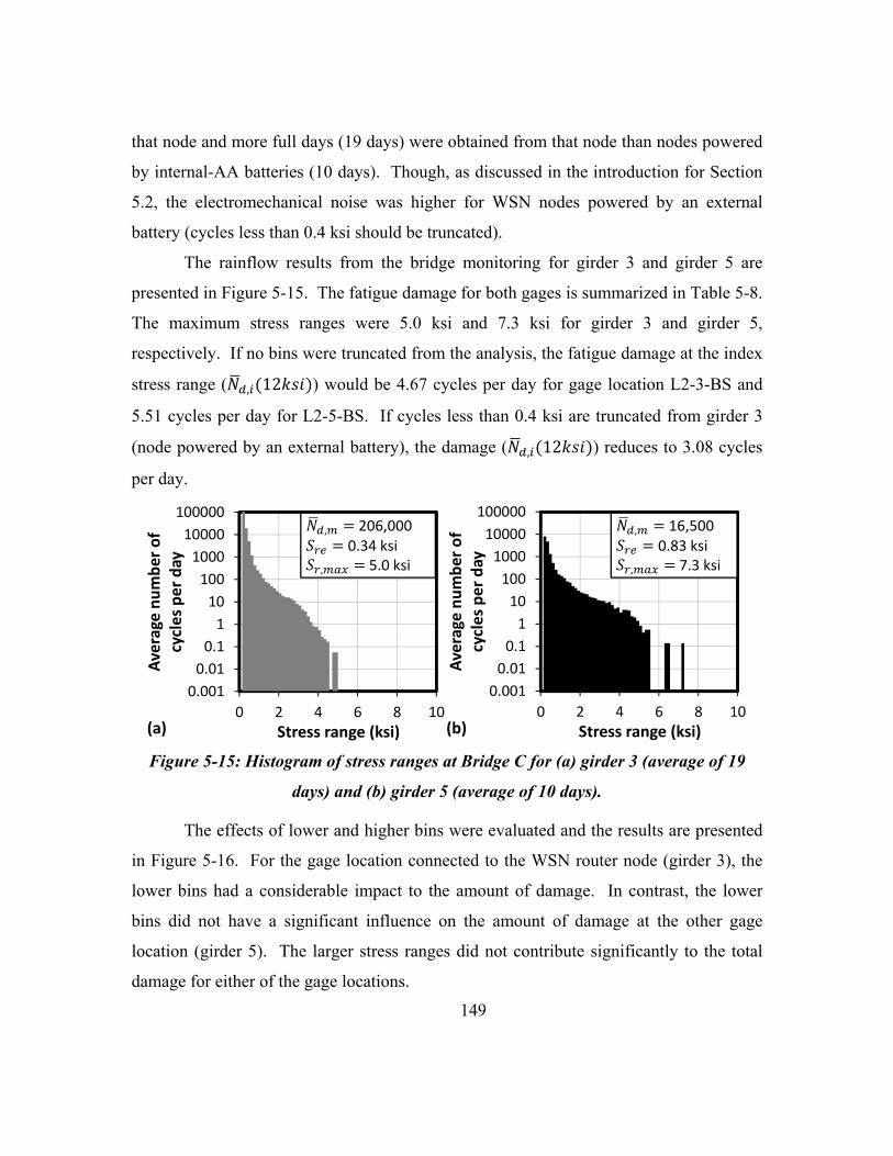
149

that node and more full days (19 days) were obtained from that node than nodes powered

by internal-AA batteries (10 days). Though, as discussed in the introduction for Section

5.2, the electromechanical noise was higher for WSN nodes powered by an external

battery (cycles less than 0.4 ksi should be truncated).

The rainflow results from the bridge monitoring for girder 3 and girder 5 are

presented in Figure 5-15. The fatigue damage for both gages is summarized in Table 5-8.

The maximum stress ranges were 5.0 ksi and 7.3 ksi for girder 3 and girder 5,

respectively. If no bins were truncated from the analysis, the fatigue damage at the index

stress range ( , 12 ) would be 4.67 cycles per day for gage location L2-3-BS and

5.51 cycles per day for L2-5-BS. If cycles less than 0.4 ksi are truncated from girder 3

(node powered by an external battery), the damage ( , 12 ) reduces to 3.08 cycles

per day.

Figure 5-15: Histogram of stress ranges at Bridge C for (a) girder 3 (average of 19

days) and (b) girder 5 (average of 10 days).

The effects of lower and higher bins were evaluated and the results are presented

in Figure 5-16. For the gage location connected to the WSN router node (girder 3), the

lower bins had a considerable impact to the amount of damage. In contrast, the lower

bins did not have a significant influence on the amount of damage at the other gage

location (girder 5). The larger stress ranges did not contribute significantly to the total

damage for either of the gage locations.

0.001

0.01

0.1

1

10

100

1000

10000

100000

0 2 4 6 8 10

Ave

rage

nu

mb

er o

f cy

cle

s p

er

day

Stress range (ksi)

0.001

0.01

0.1

1

10

100

1000

10000

100000

0 2 4 6 8 10

Ave

rage

nu

mb

er o

f cy

cle

s p

er

day


206,0000.34 ksi

5.0 ksi

16,5000.83 ksi

7.3 ksi

(b)

150

Table 5-8: Summary of average daily fatigue damage at Bridge C.


, ,

L2-3-BS (Girder 3) 7,300* 0.90 ksi* 3.08* L2-5-BS (Girder 5) 16,500 0.83 ksi 5.51


Unlike Bridges A and B, the fatigue response of Bridge C was not dominated by a

narrow band of stress ranges. Instead, the entire spectrum of stress ranges contributed to

the fatigue response of Bridge C. Therefore, no specific stress range (or set of trucks)

dominated the response at Bridge C.

Figure 5-16: Contribution of each bin to , at Bridge C for gages at girder 3

and girder 5.

The cumulative damage for both gage locations without any truncation is shown

in Figure 5-17. For girder 3, stress ranges less than 1 ksi contributed significantly to the

fatigue damage. In contrast, the accumulation of damage at girder 5 was much more

gradual (Figure 5-17(b)). The effect of the higher bins was insignificant as stress ranges

greater than 3.7 ksi for girder 3 and 5.4 ksi for girder 5 contributed only 2.5% of the

overall damage.

0

0.1

0.2

0.3

0.4

0.5


Co

ntr

ibu

tio

n t

o

Girder 3

Girder 5

4.7 cycles (L2-3-BS)


151

Figure 5-17: The cumulative fatigue damage at Bridge C for gages at (a) girder 3 and

(b) girder 5.

5.2.5 Bridge D

Due to the short installation period, only four full days of data were captured at

Bridge D. The two strain gages discussed in this section are located in the middle of span

2 (Location 1) on the bottom flange of girders 2 and 3. For the remainder of this section,

L1-2-BS and L1-3-BN are referred to as the gages on girder 2 and girder 3, respectively.

The rainflow results from the monitoring period are presented in Figure 5-18 for

girders 2 and 3. As can be seen in Table 5-9, the fatigue damage for both girders is

similar; however, the maximum stress range was 7.2 ksi for girder 2, whereas it was 4.9

ksi for girder 3.

Another strain gage was installed near the gage on girder 2 and was connected to

a CompactRIO. The histogram data from the CompactRIO are presented in Chapter 3

(Figure 3-17). Whereas many problems were identified with cycles in the higher bins in

the CompactRIO system, the larger cycles were much smaller with the WSN system.

The larger cycles for the CompactRIO were attributed to spikes in the data acquisition

system from lightning strikes. Because the WSN system was better grounded than the

CompactRIO and had shorter cables for the gages, the WSN system was not affected by

the lightning spikes.


0

0.2

0.4

0.6

0.8

1

0 2 4 6 8 10

Ave

rage

dai

ly

cum

ula

tive

dam

age


0.1 ksi

5.0 ksi 7.3 ksi

95% of damage 2.5% of

damage

0.4 ksi

3.7 ksi

95% of damage

2.5% of damage 5.4 ksi

152

Figure 5-18: Histogram of stress ranges at Bridge D (average of 4 days) for gage

locations along (a) girder 2 and (b) girder 3.

Table 5-9: Summary of average daily fatigue damage at Bridge D.


, , L1-2-BS (Girder 2) 150,000 0.60 ksi 18.8 L1-3-BN (Girder 3) 125,000 0.63 ksi 17.7

The effect of electromechanical noise (lower bins) and larger cycles (potential

spikes) were evaluated and the results are presented in Figure 5-19. As can be seen,

electromechanical noise did not contribute much to the damage accumulation at this

bridge. For girder 3, there was a large peak in the data around 2.5 ksi, whereas there

were two peaks (1.8 ksi and 3.2 ksi) in the data for location girder 2. The larger cycles

did not contribute much to the damage accumulation either.

0.001

0.01

0.1

1

10

100

1000

10000

100000

0 2 4 6 8 10

Ave

rage

nu

mb

er o

f cy

cle

s p

er

day

Stress range (ksi)

0.001

0.01

0.1

1

10

100

1000

10000

100000

0 2 4 6 8 10

Ave

rage

nu

mb

er o

f cy

cle

s p

er

day


150,000

7.2 ksi

125,000

4.9 ksi

153

Figure 5-19: Contribution of each bin to , at Bridge D for gages attached

to girders 2 and 3.

The cumulative damage for both gage locations is shown in Figure 5-20. For both

gages, electromechanical noise was not a problem, as cycles less than 0.4 ksi contributed

approximately only 2.5% of the total damage. The majority of the damage occurred

between 0.4 to 4 ksi. The higher bins (greater than 4 ksi) contributed approximately only

2.5% of the overall damage.

Figure 5-20: The cumulative fatigue damage at Bridge D for gages attached to (a)

girder 2 and (b) girder 3.

0

1

2

3


Co

ntr

ibu

tio

n t

o Girder 3

Girder 2

18.8 cycles (L1-2-BN)



0

0.2

0.4

0.6

0.8

1

0 2 4 6 8 10

Ave

rage

dai

ly

cum

ula

tive

dam

age


0.4 ksi

7.2 ksi 4.9 ksi

95% of damage

2.5% of damage

0.4 ksi

4.6 ksi

95% of damage

2.5% of damage 3.7 ksi

154

5.2.6 Summary of Daily Fatigue Damage at Bridges

Because the index stress range was used to evaluate the extent of fatigue damage

induced during the monitoring periods, the amount of relative damage between the

bridges can be compared easily (Table 5-10). For Bridge A, two gages (E-34s-TW and

W-34s-TW) were considered for data sets acquired before and after the construction of

the retrofit. The fatigue damage at these locations were converted to an index stress

range of 4.5 ksi (fatigue Category E). Two gages were also considered at Bridge B (W-1-

BE and W-3-BE), Bridge C (L2-3-BS and L2-5-BS), and Bridge D (L1-2-BN and L1-3-

BS), yet an index stress range of 12 ksi was used for these bridges because the critical

fatigue details corresponding to the locations of the strain gages were classified as

Category C′.

The average daily fatigue damage for the four bridges is summarized in Table

5-10. Because the welded connections used for all bridges were not classified in the

same category, Equation 3-7 was used to normalize all the data and convert the fatigue

damage to an index stress range of 4.5 ksi and fatigue category E ( , 4.5 : ).

Similarly, the data was converted to an index stress range of 12 ksi and fatigue category

C′ ( , 12 : ′ ). Either can be used to compare the relative accumulation of fatigue

damage at the four bridges.

The most damage occurred at Bridge A before the construction of the retrofit,

whereas the least damage occurred at Bridge B. Even after the construction of the

retrofit, Bridge A experienced more damage than the other bridges. Bridge D is

calculated to be the next most critical bridge; however, the average daily fatigue damage

is less than 10% of the average fatigue damage induced in Bridge A after the retrofit.

155

Table 5-10: Summary of average daily fatigue damage at four bridges.

Bridge Gage

location

Fatigue damage

, . , , . : , : ′

A (pre-retrofit)

E-34s-TW 6,070 - 6,070 1,280

A (pre-retrofit)

W-34s-TE 1,250 - 1,250 264

A (post-retrofit)

E-34s-TW 940 - 940 198

A (post-retrofit)

W-34s-TE 130 - 130 27.4

B+ W-1-BE - 1.71* 8* 1.71*

B+ W-3-BE - 3.47* 16* 3.47*

C+ L2-3-BS - 3.08* 15* 3.08*

C L3-5-BS - 4.86 23 4.86

D L1-2-BN - 18.8 89 18.8

D L1-3-BS - 17.7 84 17.7

* Cycles less than 0.4 ksi were truncated because of electromechanical noise. + WSN system was powered by an external battery.

5.3 VARIATIONS IN MEASURED FATIGUE DAMAGE

Because the rainflow analyses were performed in 30-min periods, the induced

fatigue damage can be characterized as a function of time of day and day of the week.

These short-term variations in fatigue damage can influence the required duration for

monitoring a bridge. If the short-term variations are modest, less than a day of data may

be all that is needed to characterize the long-term accumulation of fatigue damage.

However, if the damage varies with both time of day and day of the week, a longer

monitoring period may be needed to obtain reliable estimates of the accumulation rate of

fatigue damage. The variation in fatigue damage was determined in terms of the index

stress range.

156

The same gages discussed in Section 5.2 are used in this section. For Bridge A

(before and after the construction of the retrofit), W-34s-TE is referred to as the gage on

the west girder while E-34s-TW is the gage on the east girder. For Bridge B, W-1-BE

and W-3-BE are referred to as the gages in Span 1 and Span 3, respectively. For Bridge

C, L2-3-BS and L2-5-BS are referred to as the gages attached to Girder 3 and Girder 5,

respectively. Bridge D is not discussed in this section as not enough data were captured

at that bridge to establish the short-term trends.

5.3.1 Variation with Time of Day

To determine the variation in fatigue damage with time of day, all data associated

with a specific, 30-min time slot, regardless of day, were averaged. In Section 5.2, only

data from full days (24 hours of continuous data acquisition in a single day) were

analyzed. If data from a particular day were not continuous, due to starting/stopping the

program on the data acquisition system or loss of power, the data were not considered

when calculating the daily fatigue damage (Section 5.2). However, for this section, all

data were considered, even data from days for which the data acquisition system was

only active for a portion of the day. As such, the daily fatigue cycles discussed in this

section do not necessarily match those discussed in Section 5.2.

Besides characterizing the fatigue damage in terms of the time of day, the

rainflow data were grouped into four, six-hour time periods to evaluate variations in the

distribution of vehicles crossing the bridge. After grouping the data into the four time

periods, the contribution of each bin to the fatigue damage was calculated to determine if

differences in damage for a specific time period were caused by the number of vehicles

and/or the weight of the vehicles crossing the bridge. The four time periods were 12:00

AM to 6:00 AM (0:00-6:00), 6:00 AM to 12:00 PM (6:00-12:00), 12:00 PM to 6:00 PM

(12:00-18:00), and 6:00 PM to 12:00 AM (18:00-0:00).

157

5.3.1.1 Bridge A (Before the construction of the retrofit)

The average number of fatigue cycles at the index stress ( 4.5 ) is plotted as

a function of time of day in Figure 5-21 for the west and east girders at Bridge A before

the construction of the retrofit. As can be seen, the damage in the east girder was always

greater than that in the west girder throughout the day. The largest number of cycles

occurred in the 6-hr period between 12:00-18:00, which corresponds to when a majority

of large trucks are being driven. The least amount of damage occurred between 0:00-

6:00, when truck traffic is expected to be relatively low.

By plotting the contribution of each bin to the fatigue damage for the four, six-

hour periods (Figure 5-22), a difference in the distribution of stress ranges crossing the

bridge can be noted. The peak in damage for 12:00-18:00 occurred at approximately 7.5

ksi, whereas it occurred at 7.0 ksi for 0:00-6:00. Because the magnitudes of each

rainflow bin are larger and the curve is shifted further to the right, a greater number of

trucks crossed the bridge during the 12:00-18:00 period and those trucks were typically

heavier than the trucks that crossed during the 0:00-6:00 period. The shape of the 6:00-

12:00 curve was similar to the 12:00-18:00 curve, whereas the 18:00-0:00 curve was

similar to the 0:00-6:00 curve.

Figure 5-21: Variation in . with time of day before the construction of the


0

50

100

150

200

250

0:00 2:00 4:00 6:00 8:00 10:00 12:00 14:00 16:00 18:00 20:00 22:00 0:00Time of Day

East girder

West girder

158

Figure 5-22: Contribution of each bin to . during the specific 6-hour

periods before the construction of the retrofit for the east girder at Bridge A.

5.3.1.2 Bridge A (After the construction of the retrofit)

After the construction of the retrofit, the average variation in fatigue damage with

time of day was similar to the variation before the retrofit; however, the amplitudes of the

damage were smaller due to the benefit of the retrofit. The variation with time of day is

presented in Figure 5-23 for the west and east girders. As it did before the retrofit (Figure

5-22), the most damage occurred between 12:00-18:00. Similarly, before the retrofit, the

trucks that crossed from 12:00-18:00 were heavier and in greater number than the trucks

that crossed during the 0:00-6:00 (Figure 5-24).

Figure 5-23: Variation in . with time of day after construction of the


0

40

80

120

160

0 5 10 15 20 25Stress Range (ksi)

Average

0:00-6:00

6:00-12:00

12:00-18:00

18:00-24:00

Co

ntr

ibu

tio

n t

o

Between 12:00-18:00

Between 18:00-0:00

Average

Between 0:00-6:00

Between 6:00-12:00

Number of cycles (for 6-hour period):0:00-6:00: 7106:00-12:00: 1,29012:00-18:00: 2,30018:00-0:00: 1,580Average: 1,470

0

10

20

30

40

50

0:00 2:00 4:00 6:00 8:00 10:00 12:00 14:00 16:00 18:00 20:00 22:00 0:00Time of Day

West girder

East girder

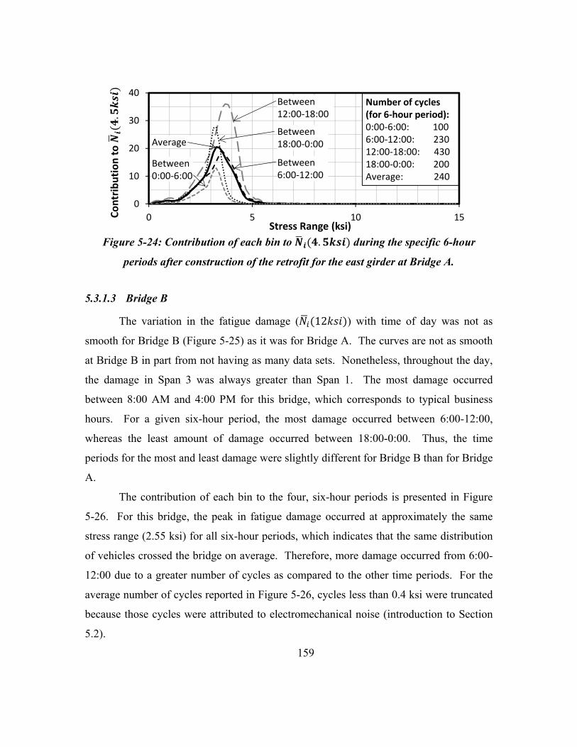
159

Figure 5-24: Contribution of each bin to . during the specific 6-hour

periods after construction of the retrofit for the east girder at Bridge A.

5.3.1.3 Bridge B

The variation in the fatigue damage ( 12 ) with time of day was not as

smooth for Bridge B (Figure 5-25) as it was for Bridge A. The curves are not as smooth

at Bridge B in part from not having as many data sets. Nonetheless, throughout the day,

the damage in Span 3 was always greater than Span 1. The most damage occurred

between 8:00 AM and 4:00 PM for this bridge, which corresponds to typical business

hours. For a given six-hour period, the most damage occurred between 6:00-12:00,

whereas the least amount of damage occurred between 18:00-0:00. Thus, the time

periods for the most and least damage were slightly different for Bridge B than for Bridge

A.

The contribution of each bin to the four, six-hour periods is presented in Figure

5-26. For this bridge, the peak in fatigue damage occurred at approximately the same

stress range (2.55 ksi) for all six-hour periods, which indicates that the same distribution

of vehicles crossed the bridge on average. Therefore, more damage occurred from 6:00-

12:00 due to a greater number of cycles as compared to the other time periods. For the

average number of cycles reported in Figure 5-26, cycles less than 0.4 ksi were truncated

because those cycles were attributed to electromechanical noise (introduction to Section

5.2).

0

10

20

30

40

0 5 10 15Stress Range (ksi)

Average

0:00-6:00

6:00-12:00

12:00-18:00

18:00-24:00

Co

ntr

ibu

tio

n t

o

Between 12:00-18:00

Between 18:00-0:00Average

Between 0:00-6:00

Between 6:00-12:00

Number of cycles (for 6-hour period):0:00-6:00: 1006:00-12:00: 23012:00-18:00: 43018:00-0:00: 200Average: 240

160

Figure 5-25: Variation in with time of day at Bridge B (cycles less than 0.4

ksi were truncated).

Figure 5-26: Contribution of each bin to during the specific 6-hour periods

for Span 1 at Bridge B.

5.3.1.4 Bridge C

As with the variation with time of day observed for Bridge B, the variation in

fatigue damage at Bridge C was not very smooth (Figure 5-27). The damage at girder 5

was slightly greater than girder 3 during the middle of the day. Similar to Bridge B, the

most damage occurred between 8:00 AM and 4:00 PM for this bridge. For a given six-

hour period, the most damage occurred between 12:00-18:00, whereas the least amount

of damage occurred between 0:00-6:00. Due to the high electromechanical noise at

girder 3, cycles less than 0.4 ksi were truncated for that location only in Figure 5-27.

0.00

0.04

0.08

0.12

0.16

0:00 2:00 4:00 6:00 8:00 10:00 12:00 14:00 16:00 18:00 20:00 22:00 0:00Time of Day

Span 3

Span 1

0.00

0.02

0.04

0.06

0.08

0.10


Average

0:00-6:00

6:00-12:00

12:00-18:00

18:00-24:00

Co

ntr

ibu

tio

n t

o

Between 6:00-12:00

Between 12:00-18:00

Average

Between 0:00-6:00 Between

18:00-0:00

Number of cycles (for 6-hour period):0:00-6:00: 0.30*6:00-12:00: 0.66*12:00-18:00: 0.51*18:00-0:00: 0.23*Average: 0.42**Cycles less than 0.4 ksiwere truncated from sum

161

Figure 5-27: Variation in with time of day at Bridge C (cycles less than 0.4

ksi were truncated for girder 3 only).

The contribution of each bin for four, six-hour periods is presented in Figure 5-28.

For this bridge, the peak in fatigue damage occurred between 3-4 ksi during the middle of

the day (6:00-12:00 and 12:00-18:00). In contrast, the peaks occurred between 2-3 ksi

for night periods (0:00-6:00 and 18:00-0:00). As such, the data indicated a higher

number of heavier trucks during the daylight hours as compared to night.

Figure 5-28: Contribution of each bin to during the specific 6-hour periods

for girder 5 at Bridge C.

5.3.2 Variation with Day of the Week

The variation in fatigue damage as a function of the day of the week was

evaluated by considering only data from full days (24 hours in a single day). For each

0.00

0.05

0.10

0.15

0.20

0.25

0.30

0:00 2:00 4:00 6:00 8:00 10:00 12:00 14:00 16:00 18:00 20:00 22:00 0:00Time of Day

Girder 5

Girder 3

0.00

0.05

0.10

0.15

0.20


Average

0:00-6:00

6:00-12:00

12:00-18:00

18:00-24:00

Co

ntr

ibu

tio

n t

o

Between 12:00-18:00

Between 6:00-12:00

Average

Between 0:00-6:00

Between 18:00-0:00

Number of cycles (for 6-hour period):0:00-6:00: 0.206:00-12:00: 1.7212:00-18:00: 2.0718:00-0:00: 0.34Average: 1.09

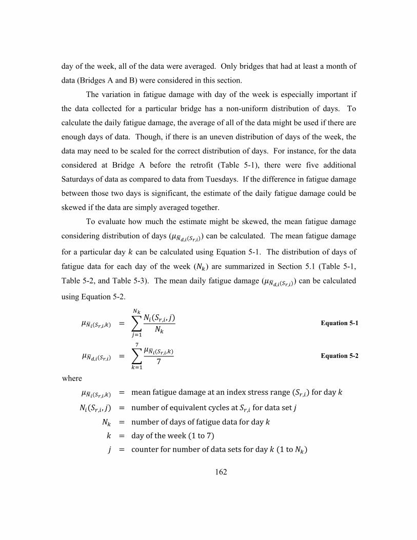
162

day of the week, all of the data were averaged. Only bridges that had at least a month of

data (Bridges A and B) were considered in this section.

The variation in fatigue damage with day of the week is especially important if

the data collected for a particular bridge has a non-uniform distribution of days. To

calculate the daily fatigue damage, the average of all of the data might be used if there are

enough days of data. Though, if there is an uneven distribution of days of the week, the

data may need to be scaled for the correct distribution of days. For instance, for the data

considered at Bridge A before the retrofit (Table 5-1), there were five additional

Saturdays of data as compared to data from Tuesdays. If the difference in fatigue damage

between those two days is significant, the estimate of the daily fatigue damage could be

skewed if the data are simply averaged together.

To evaluate how much the estimate might be skewed, the mean fatigue damage

considering distribution of days (, ,

) can be calculated. The mean fatigue damage

for a particular day can be calculated using Equation 5-1. The distribution of days of

fatigue data for each day of the week ( ) are summarized in Section 5.1 (Table 5-1,

Table 5-2, and Table 5-3). The mean daily fatigue damage (, ,

) can be calculated

using Equation 5-2.

, , , , Equation 5-1

, , , ,

7 Equation 5-2

where

, , meanfatiguedamageatanindexstressrange , forday

, , numberofequivalentcyclesat , fordataset

numberofdaysoffatiguedataforday

dayoftheweek 1to7

counterfornumberofdatasetsforday 1to

163

, , meanfatiguedamageconsideringdistributionofdaysatan

indexstressrange ,

5.3.2.1 Bridge A (Before the construction of the retrofit)

For the period before the retrofit at Bridge A (Table 5-1), the average variation in

fatigue damage ( , 4.5 ) with day of the week for the west and east girders is

presented in Figure 5-29. As can be seen, more damage occurred on weekdays than

weekends due to the larger volume of trucks that travel on the weekdays compared to

weekends. On average, the maximum amount of damage occurred on Tuesday at this

bridge. If the damage for Monday through Friday is compared to the damage on Sunday,

the damage for the weekday is 2.3 to 2.8 times greater than the damage on Sunday in the

west girder and 1.9 to 2.2 times greater in the east girder.

Figure 5-29: Average variation of fatigue damage ( , . ) for the west and east

girders before the construction of the retrofit at Bridge A.

The average daily fatigue damage before the construction of the retrofit is

summarized for the west and east girders (Table 5-11). The data indicate that there is not

much difference between accounting for the distribution of days (, . ) and

average of all full days of data ( , 4.5 ). The small difference is likely due to the

6,172

7,314 7,207 7,005 6,793

4,852

3,280

1,313 1,578 1,454 1,406 1,4331,006

572

0

2,000

4,000

6,000

8,000

10,000

Mon Tue Wed Thu Fri Sat Sun

East Girder

West Girder

(9 days) (8 days) (12 days)Days of data: (10 days) (10 days) (13 days) (9 days)

164

large amount of measured data (71 days for most gages). In addition, of the 71 days, the

distribution of the weekdays (5 out of 7) and weekend days (2 out of 7) is nearly correct.

Table 5-11: Summary of daily fatigue damage before the construction of the retrofit at

Bridge A.

Gage Mean fatigue damage based

on distribution of days (

, . )

Average of days monitored

( , . )

W-34s-TE (West girder) 1,250 1,250 E-34s-TW (East girder) 6,090 6,070

5.3.2.2 Bridge A (After the construction of the retrofit)

The variation in fatigue damage as a function of day of the week was similar after

the construction of the retrofit at Bridge A (Figure 5-30) as it was before the retrofit. As

previously, more damage occurred on weekdays than weekends. The most damage

occurred on Tuesday for the east girder, whereas it occurred on Wednesday for the west

girder. If the damage for Monday through Friday was compared to the damage on

Sunday, the damage for the weekday was 1.4 to 1.9 times greater for the west girder and

1.7 to 2.0 times greater for the east girder than the damage on Sunday.

Figure 5-30: Variation of fatigue damage ( , . ) for the west and east girders

after construction of the retrofit at Bridge A.

947

1,102 1,070 1,066 1,035

800

547

126 142 160 146 140 125 82

0

500

1,000

1,500


East Girder

West Girder

(25 days) (28 days) (27 days)Days of data: (24 days) (27 days) (28 days) (27 days)

165

The distribution of days monitored after the construction of the retrofit was fairly

uniform (Table 5-2); therefore, the estimate of the daily fatigue damage was similar

whether the distribution of days were used or the average of all the days monitored

(Table 5-12).

Table 5-12: Summary of daily fatigue damage after construction of the retrofit at

Bridge A.

Gage Mean fatigue damage based on distribution of days (

, . )


( , . )

W-34s-TE (West girder) 130 130 E-34s-TW (East girder) 938 940

5.3.2.3 Bridge B

The average variation of damage with the day of the week was determined for

Span 1 and Span 3 (Figure 5-31). As with Bridge A, the fatigue damage from a weekday

was greater than a weekend at Bridge B. For Span 1, there was no variation in fatigue

damage between Monday and Friday. In contrast, there was some variation in the fatigue

damage in Span 3, with the most damage on average occurring on Monday.

Figure 5-31: Variation of fatigue damage ( , ) for Span 1 and Span 3 at

Bridge B (cycles less than 0.4 ksi were truncated).

2.0 2.0 2.1 2.0 2.0

1.30.7

4.4 4.23.6

4.0 3.9

2.6

1.5

0

1

2

3

4

5

6


Span 1

Span 3

166

Because a fairly uniform distribution of data was collected at Bridge B (Table

5-3), there was not expected to be much skew between considering the distribution of

days and simply calculating the average. As seen in Table 5-13, there is not much

difference between the two methods of calculating the daily fatigue damage.

Table 5-13: Summary of daily fatigue damage after construction of the retrofit at

Bridge A.

Gage Mean fatigue damage based

on distribution of days (

,)


( , )

W-1-BE (Span 1) 1.72* 1.71* W-3-BE (Span 3) 3.44* 3.47*

* Cycles less than 0.4 ksi were truncated

5.3.3 Weekly

One set of researchers recommended that a bridge should be monitored

continuously for two to four weeks to obtain an accurate representation of the damage

(Connor and Fisher 2006). To evaluate that recommendation, the weekly variation in

fatigue damage was determined at Bridge A for the period after the construction of the

retrofit. The gage was attached to the bottom flange of the east longitudinal girder near

floor beam 35 (E-35n-BE) (Figure 5-32). The damage from seven continuous days of

monitoring was averaged to obtain and estimate the average amount of daily damage

( , 4.5 ).

The average daily damage for all of the data is 6,000 cycles per day. For each

individual week, the damage was within 10% (600 cycles) of the average except for

weeks that included a federal holiday. Thus, one continuous week of data provided an

adequate representation of data for this gage location as long as the week did not contain

a holiday. However, because estimating the remaining fatigue life involves forecasting

the damage, 10% error in the damage may have a significant impact on the calculated

fatigue life.

167

Figure 5-32: Variation in average daily damage ( , . ) due to a week of

continuous monitoring for gage E-35n-BE at Bridge A.

The variation in weekly damage for a gage attached to the top flange of the east

longitudinal girder near floor beam 34 (E-34s-TW) is presented in Figure 5-33. For this

location, the average of all the data was 945 cycles per day. There was more variation in

the weekly damage at this location, such that an individual week of data could cause as

much as 20% difference in damage (excluding weeks with a federal holiday).

Figure 5-33: Variation in average daily damage ( , . ) due to a week of

continuous monitoring for gage location E-34s-TW at Bridge A.

The data in Figure 5-33 suggest that there could be a variation in damage from

month to month. For instance, the damage ( , 4.5 ) from 3/1/2012 to 5/31/2012

had a daily average of 1,040 cycles, whereas the damage was reduced from 6/1/2012 to

7/30/2012 with a daily average of 810 cycles.

5000

5500

6000

6500

7000

Date

Each data point is the average of seven continuous days of monitoring

Average Week had a holiday

Average ±10%

500

1000

1500

Date

Week had a holiday

Each data point is the average of seven continuous days of monitoring

Average

±20%

168

5.3.4 Summary of Variation in Measured Fatigue Response

Due to the weekly, daily, and hourly variation in damage, a continuous week of

data should be collected as the minimum monitoring period. Monitoring for only part of

the day or week will not be representative of the true damage at the bridge. If calculating

the remaining fatigue life is desired, four weeks of data is recommended to make long-

term projections. Because damage may vary month to month, a permanent monitoring

system could be installed at a bridge and data could be collected for one to two weeks

every month for the entire year.

5.4 TRACKING PROGRESS OF CONSTRUCTION AT BRIDGE A

The construction of the retrofit at Bridge A took place from 8/29/2011 to

11/18/2011. Because the index stress range was used to convert the distribution of stress

ranges into normalized fatigue damage, the progress of repairing cracked connections

could be tracked. The results from four gage locations are discussed in this section. The

results for the other gage locations can be found in Appendix A. Of the gages used to

measure the fatigue of the bridge during the initial acquisition period, some gages were

destroyed during construction and were replaced after completion of the construction.

For most of the gages, 57 full days of data were obtained during the retrofit. In the north

span, only the regions around floor beams 34 to 38 of both longitudinal girders were

retrofitted (Section 4.1.3).

Six strain gages will be discussed in this section. Gage W-35s-BW was installed

on the west side of the bottom flange of the west longitudinal girder near the connection

to floor beam 35, whereas gage E-35n-BW was installed on west side of the bottom

flange of the east longitudinal girder near floor beam 35. W-35s-BW will be referred to

as the bottom flange on the west girder and E-35n-BW will be referred to as the bottom

flange on the east girder. For gages installed along the longitudinal girders near floor

beam 34, W-34s-TE will be referred to as the top flange of the west girder and E-34s-TW

will be referred to as the top flange of the east girder. Finally, two gages were installed

on the east longitudinal girder near floor beam 27. E-27-TW will be referred to as the top

169

flange at floor beam 27 and E-27-BW will be referred to as the bottom flange at floor

beam 27.

5.4.1 Rainflow Results

The average daily cycles of stress ranges for the construction period of the retrofit

for the gages attached to the bottom flanges are presented in Figure 5-34. Similar to the

period before the construction of the retrofit, the effect of the lower (electromechanical

noise) and higher (data acquisition spikes) bins were minimal and did not need to be

truncated. The maximum stress ranges were 23.6 ksi and 16.7 ksi for the bottom flanges

of the west and east girders, respectively. The histograms of stress ranges for gages

attached to the top flanges are presented in Figure 5-35. The maximum stress ranges

were 18.5 ksi and 11.2 ksi for the bottom flanges of the west and east girders,

respectively.

Figure 5-34: Histogram of stress ranges during the construction of the retrofit

(average of 57 days) for gages on the bottom flanges of the (a) west and (b) east

girders.

0.001

0.01

0.1

1

10

100

1000

10000

100000

0 10 20 30

Ave

rage

nu

mb

er o

f cy

cle

s p

er

day

Stress range (ksi)

0.001

0.01

0.1

1

10

100

1000

10000

100000

0 10 20 30

Ave

rage

nu

mb

er o

f cy

cle

s p

er

day


141,000

23.6 ksi

143,000

16.7 ksi

170

Figure 5-35: Histogram of stress ranges during the construction of the retrofit

(average of 57 days) for gages on the top flanges of the (a) west and (b) east girders.

5.4.2 Behavior of Bridge During Construction

The characterization of fatigue damage is not as interesting during the

construction of the retrofit because a new detail will be assumed once the construction is

finished. However, by plotting the fatigue damage on a daily basis using the index stress

range, changes in the traffic pattern due to the construction of the retrofit can be

identified. This is an added benefit of using the index stress range to represent the daily

fatigue damage. If the effective stress range were plotted on a daily basis, the changes in

the traffic pattern would not be as readily identified.

To construct the retrofit, one lane was closed at a time so that the concrete deck

could be removed and the cover plates installed at the appropriate floor beam locations

(Figure 4-9). The contractor started with the east girder, which corresponds to the right

lane. Construction along the east girder took place from August 29 until November 6.

Part of the right lane was reopened at that time and the contractor moved to the west

girder and closed the left lane (traffic could cross the bridge along the second bridge at

the site—for exit ramp). The retrofit construction for the west girder went much quicker,

and was completed on November 18.

0.001

0.01

0.1

1

10

100

1000

10000

100000

0 10 20 30

Ave

rage

nu

mb

er o

f cy

cle

s p

er

day

Stress range (ksi)(b)

0.001

0.01

0.1

1

10

100

1000

10000

100000

0 10 20 30

Ave

rage

nu

mb

er o

f cy

cle

s p

er

day


48,400

18.5 ksi

55,100

11.2 ksi

171

The daily fatigue damage ( , 4.5 ) for the gages on the bottom flanges are

shown in Figure 5-36. Each phase of the construction period can be identified in the

graph. Before the retrofit, the fatigue damage in the bottom flange of the east girder was

larger than bottom flange of the west girder because more trucks would be expected to

pass in the right lane (east girder) when both lanes are opened. With the right lane

closed, the damage accumulation in the east girder decreased to almost zero, whereas the

damage accumulation at the gage location on the west girder increased substantially.

Because all trucks had to cross the bridge in the left lane when the right lane was closed,

the damage accumulation in the west girder increased almost to the same level as the east

girder before construction. When part of the right lane was reopened and the left lane

was closed, the accumulation of fatigue damage in the west girder decreased to almost

zero. After construction was finished on both girders, the accumulation of damage

measured in the bottom flange of the east girder was larger than the west girder.

However, the values in the bottom flanges were slightly smaller than the values before

the retrofit.

Figure 5-36: Daily fatigue damage ( , . ) during the construction process for

the bottom flanges in the west and east girders at Bridge A.

The daily fatigue damage ( , 4.5 ) for the top flanges near floor beam 34

are shown in Figure 5-37. The accumulation of damage in the top flanges was similar to

0

4,000

8,000

12,000

16,000

Date

E-35n-BWW-35s-BW

B

A. Prior to retrofitB. Right (east) lane closed

A

C. Left (west) lane closedD. Retrofit completed

C D

172

the damage in the bottom flange. When the right lane was closed, the accumulation of

damage in the top flange of the east girder was nearly zero, whereas the accumulation of

damage in the top flange of the west girder increased substantially. When part of the

right lane was reopened and the left lane was closed, the accumulation of fatigue damage

in the top flange of the west girder decreased to almost zero. After the bridge was

reopened, the accumulation of damage in the top flange of the east girder was again

larger than the west girder. Nonetheless, the retrofit greatly reduced the growth rate of

fatigue damage in the top flanges.


the top flanges in the west and east girders at Bridge A.

Because the fatigue damage in the top flanges is nearly zero and much larger in

the bottom flanges, the behavior is similar to composite action between the concrete deck

and steel longitudinal girder. Before the retrofit, the contribution of the top and bottom

flanges was similar in the east girder (Figure 5-38(a)). After the retrofit, the contribution

of the bottom flange is much larger than the top flange (Figure 5-38(b)). The composite

action is believed to have been created by the bolts from the retrofit plates extending into

the concrete deck (Figure 4-12). The composite action was unintentional as the retrofit

detail was not specifically designed for composite action. As such, the detail should be

monitored that the stress reduction in the top flanges continues to occur over time.

0

2,000

4,000

6,000

8,000

Date

E-34s-TWW-34s-TW

B


A


C D

173

Figure 5-38: Contribution to fatigue damage for the top and bottom flanges in the east

girder of Bridge A (a) before and (b) after construction of the retrofit.

Strain gages were added to the retrofit plates at floor beam 34 after the

construction process. The gages indicated that the retrofit plates were not carrying much

of the load, such that the fatigue damage from the retrofit plate barely shows up in Figure

5-39. The low number of fatigue cycles ( , 4.5 ) in the top flanges and the retrofit

plates after construction emphasizes the benefit of the partial composite action between

the concrete deck and longitudinal girder.

Figure 5-39: Contribution to fatigue damage for the top flange of the east girder and

retrofit plate at Bridge A.

0

100

200

300

400

500


0

100

200

300

400

500


Bottom flange

Co

ntr

ibu

tio

n t

o

Top flange

Co

ntr

ibu

tio

n t

o

(a) (b)

Top flange

Bottom flange

0

20

40

60

80

100

0 1 2 3 4 5 6Stress range (ksi)

Before construction

Co

ntr

ibu

tio

n t

o After

construction

Retrofit plate

174

Floor beam 34 was the last location that was retrofitted on the north span. At

floor beam 27, the gages were monitored for the period before construction, during

construction, and for a couple days after construction (Figure 5-40). The response of the

gages near floor beam 27 was similar to the gages near floor beam 35 during construction

of the retrofit. However, while there was a significant reduction in the fatigue damage in

the top flanges and slight reduction in the bottom flanges at the retrofit locations, the

fatigue damage after construction at the locations near floor beam 27 were similar to the

fatigue damage before construction. Therefore, the retrofit did not generally provide a

measureable benefit at locations away from the retrofit locations.


the east longitudinal girder near floor beam 27 at Bridge A.

5.5 SUMMARY

Strain data from four bridges were analyzed using the techniques presented in

Chapter 3. The details of the bridges were discussed in Chapter 4. Using the

visualization techniques (contribution to damage (Section 3.3.1) and cumulative damage

(Section 3.3.2)), the spectra of stress ranges for each bridge were verified (Section 5.2).

The lower and higher bins did not significantly influence the total fatigue damage if the

cycles were load induced. If cycles corresponding to electromechanical noise were not

0

200

400

600

800

1,000

Date

E-27s-TWE-27s-BW

B


A


C D

175

truncated from the rainflow histograms (Bridges B and C), then the contribution to

damage of the lower bins was very large and caused steep steps in how each rainflow bin

contributed to the cumulative damage. Similarly, if the higher bins were due to spikes in

the data acquisition system, considering those bins would lead to erroneous indications of

damage that would lead to overestimating the fatigue damage for the monitoring period

(Figure 5-10). Cycles corresponding to electromechanical noise or spikes in the data

acquisition system should be truncated from the rainflow histogram because they do not

induce fatigue damage.

Using the index stress range, the average daily fatigue damage was computed for

each bridge to allow comparison of the relative accumulation of fatigue damage (Section

5.2.6). If the details from each bridge correspond to different fatigue categories, all of the

data should be normalized to a specific detail category using Equation 3-7. By

normalizing to the same index stress range and fatigue category, the relative

accumulation can be compared directly. Bridge A was the most critical of the four

bridges based on relative accumulation of fatigue damage.

The variation in fatigue damage as a function of time of day and day of the week

was evaluated for the bridges (Section 5.3). The fatigue damage varied both hourly and

daily, such that the minimum monitoring period should be a continuous week of data.

However, due to weekly variations in the fatigue damage, a minimum of four weeks of

data are needed to make long-term projections of fatigue damage for the purpose of

calculating the remaining fatigue life.

An added value of using the index stress range to characterize fatigue damage was

exemplified by tracking the progress of the construction of the retrofit at Bridge A

(Section 5.4). Each phase of construction could be identified using the index stress

range. Additionally, the benefit of the retrofit was immediately apparent from the

reductions in the daily fatigue damage.

176

CHAPTER 6

Comparison of the Calculated and Measured

Responses of Bridge A

The calculation of the remaining fatigue life of a connection or component of a

steel bridge relies on an engineer evaluating the fatigue damage at a specific point in

time. The fatigue damage can be estimated by field monitoring or combining structural

analysis with standard traffic counts and design values from the AASHTO LRFD

Specifications (2010). If a structural-analysis approach is chosen, an engineer must

assume a representative fatigue truck, live load distribution among the girders, and

dynamic impact factor to calculate the effective stress range. The suggested design

values from AASHTO may not provide an accurate representation of the service-load

conditions for a particular bridge, leading to unreliable estimates of the fatigue damage.

The distribution of stress ranges under service loads is measured directly when a bridge is

monitored, which reduces the uncertainty associated with the calculated fatigue damage.

A live load test was conducted at Bridge A to compare the assumed design values

utilized in a structural-analysis approach with values obtained from field monitoring.

Specifically, a load test was conducted to determine the effect of vehicle speed and lane

position on the bridge behavior. Based on the field data, a measure of the girder

distribution factor and dynamic impact factor were obtained. The distribution of the

measured stress ranges was compared to the assumed distribution of trucks crossing the

bridge based on the AASHTO fatigue truck. Details of Bridge A are discussed in

Chapter 4. This load test occurred prior to the construction of the retrofit.

6.1 BENDING-STRESS HISTORIES

The load test was performed in July 2011 by driving a single truck across the

bridge to determine the effects of vehicle speed and lane position. A rolling road block

was used to isolate the bridge from other traffic, while minimizing delays to the traveling

177

public. The rolling road block consisted of a test truck entering the freeway followed by

two trailing vehicles. The trailing vehicles traveled at a reduced speed in adjacent lanes

to create a gap (0.25 to 0.5 miles) between the test truck and normal traffic. With gaps

behind and in front of the test truck, it was the only vehicle crossing the bridge during the

test.

The test truck crossed the bridge in various lane positions to determine the

stresses imposed in each girder for different transverse positions. The axle spacings and

weights of the test truck (total weight of approximately 65 kips) are listed in Figure 6-1.

The bridge is currently striped for two traffic lanes (Figure 4-4). The truck was driven in

the right and left lanes at 10 mph, 30 mph, and 63 mph. In addition, the truck was driven

over a proposed new center lane at 10 mph and 30 mph (Figure 6-2). The center lane was

a potential retrofit to combine the two lanes into a single lane to reduce the stress ranges

on the twin-girder structure until a replacement bridge could be designed and constructed.

When a vehicle crosses the bridge in the right lane, most of the load is transferred to the

east girder. Likewise, when a vehicle crosses the bridge in the left lane, most of the load

is transferred to the west girder. The proposed center lane provided a more uniform load

distribution between the girders.

Figure 6-1: Truck weight and spacing of axles.

Strain gages were installed on both sides of the top and bottom flanges to isolate

the stresses from flexural bending and warping torsion (lateral bending of the flanges).

The stresses from flexural bending and warping torsion can be approximated by using

6′-10″ 6′-0″17-9″

19.6kips

18.8 kips

W = 64.9 kips18.8 kips

7.7kips

4′-6″

178

superposition as demonstrated in Figure 6-3. The bending stresses are obtained from the

average of the two readings while the warping stresses are obtained from the difference

between the two readings.

Figure 6-2: Proposed new center lane for Bridge A.

Figure 6-3: Isolation of flexural bending and flange warping stresses.

The bending stress histories of the east and west longitudinal girders at floor beam

34 due to the test truck crossing the bridge at 10 mph are shown in Figure 6-4. For the

purposes of the live load test, this speed was assumed to be representative of a static test.

The static assumption is reasonable because the data show a single, large-cycle stress

range with few secondary stress cycles associated with the dynamic excitation of the

bridge. As expected, when the truck was in the left lane (Figure 6-4(a)), the west girder

experienced a larger stress range (8.0 ksi) than the east girder (4.3 ksi). Conversely, the

4′-0″6′-1½″


(proposed center lane)

6′-0″8′-6″ 8′-6″

Strain gage

179

stress range in the east girder (9.1 ksi) was larger than the west girder (2.5 ksi) when the

truck was the right lane (Figure 6-4(b)).

Figure 6-4: Flexural stress history in top flange of east and west girders at floor beam

34 due to test truck crossing the bridge at 10 mph in the (a) left lane and (b) right lane.

When the truck crossed the bridge at higher speeds, there was a noticeable change

in the stress history (Figure 6-5). At 63 mph, in addition to the single, large stress cycle,

there were many secondary cycles due to vibration of the bridge. The secondary cycles

were due to dynamic effects from the bridge vibrating as the truck crossed the bridge and

excitation of the truck suspension. At the higher speeds, the flexural stress range was

larger than the measured values for the slower speeds (8.8 ksi (west girder) and 5.3 ksi

(east girder) for a truck crossing in the left lane and 11.1 ksi (east girder) and 5.1 ksi

(west girder) for a truck crossing in the right lane).

The secondary cycles observed in Figure 6-5 increase the fatigue damage as

compared to considering only the primary stress cycle. To calculate the additional

damage, the spectrum of stress ranges from each truck crossing the bridge must be

identified using the rainflow algorithm. For example, the flexural stress ranges identified

in the top flange of the east longitudinal girder near floor beam 34 due to a truck crossing

the bridge in the left and right lanes at 30 mph are summarized in Figure 6-6. As

discussed in Chapter 3, the fatigue damage from the truck crossing the bridge can be

0 4 8 12 16Time (sec)

-6.0

-4.0

-2.0

0.0

2.0

4.0

6.0

0 4 8 12 16

Flex

ura

l str

ess

(ksi

)

Time (sec)

East girder

West girder

Truck in right lane (10 mph)Truck in left lane (10 mph)

(a) (b)

East girder

West girder

180

represented by the index stress range or the effective stress range. Alternatively, the

truck crossing the bridge can be related to a single cycle at an equivalent stress range

( 1 ), which is calculated to produce an equal amount of fatigue damage as the

spectrum of stress ranges.

Figure 6-5: Flexural stress history in top flange of east and west girders at floor beam

34 due to test truck crossing the bridge at 63 mph in the (a) left lane and (b) right lane.

Figure 6-6: Histogram of flexural stress ranges in the top flange of the east girder

near floor beam 34 due to the test truck crossing the bridge at 30 mph in the (a) left

lane and (b) right lane.

0 2 4 6 8Time (sec)

East girder

West girder

Truck in right lane (63 mph)

-6.0

-4.0

-2.0

0.0

2.0

4.0

6.0

0 2 4 6 8

Flex

ura

l str

ess

(ksi

)

Time (sec)

Truck in left lane (63 mph)

(a) (b)

East girder

West girder

(a) (b)

0

1

2

3

4

5

0 2 4 6 8 10

Nu

mb

er o

f cy

cles

Stress range (ksi)

0

1

2

3

4

5

0 2 4 6 8 10

Nu

mb

er o

f cy

cles

Stress range (ksi)

181

The damage accumulation index ( ) discussed in Section 2.2.1.1 can be used to

derive the equivalent stress range for a single truck event ( 1 ). The damage from the

spectrum of stress ranges due to the truck crossing the bridge (left side) must equal the

damage from an equivalent stress range for a single cycle (right side) as seen in Equation

6-1. The equivalent stress range for a single cycle can be calculated using Equation 6-2.

∑ 1

1 Equation 6-1

1 /

Equation 6-2

where

1 effective stress range for a single truck event

numberofcyclesinbincorrespondingto

averagestressrangeforbin

fatigueconstantfordetailcategory,definedbyAASHTOLRFDSpecifications 2010 ksi3

The equivalent stress range for a single truck event ( 1 ) was used to relate the

fatigue damage from the test truck crossing the bridge at a vehicle speed of 30 mph

(Table 6-1). As a reference, the largest stress range determined by the rainflow algorithm

is listed in parenthesis in the table. There is a slight difference between 1 and the

largest, measured stress range because the secondary, vibrational stress ranges increase

the apparent damage. At floor beam 35, the bending stresses measured for the top and

bottom flanges exhibited similar amplitudes, which indicate a lack of composite action

between the steel girders and the concrete bridge deck.

For trucks crossing the bridge in the proposed center lane, the load distribution

between the girders was nearly equal. For instance, for a test truck crossing the bridge at

30 mph, equivalent stress ranges of 6.78 ksi in the west girder and 7.19 ksi in the east

girder were recorded in the top flanges near the connection at floor beam 34 (Table 6-1).

These values are approximately 70% of the maxima when the vehicle was in the left lane

(west girder) and the right lane (east girder).

182

Table 6-1: Equivalent bending stress ranges ( ) in longitudinal girders for trucks

crossing the bridge at 30 mph.

Girder Floor beam

Flange for truck location (ksi)

Left lane Right lane Center lane East 27s Top 1.65 (1.52) 3.29 (3.26) 2.44 (2.39) East 27s Bottom 1.95 (1.81) 3.59 (3.55) 2.73 (2.68) East 34s Top 5.49 (5.44) 9.94 (9.93) 7.19 (7.18) East 35n Top 3.32 (3.26) 7.03 (7.03) 4.87 (4.86) East 35n Bottom 5.09 (5.00) 9.37 (9.35) 6.92 (6.89) East 35s Top 4.61 (4.57) 8.49 (8.48) 6.32 (6.31) West 34s Top 9.24 (9.21) 3.00 (2.97) 6.78 (6.74) West 35s Top 7.93 (7.91) 2.56 (2.54) 5.90 (5.87) West 35s Bottom 9.11 (9.06) 3.50 (3.41) 6.79 (6.74)

Value in () is the largest stress range determined by the rainflow method.

6.2 DISTRIBUTION FACTOR

At longitudinal locations where strain gages are installed on both girders, the live

load distribution factor (LLDF) can be determined from the measured data. In Chapter 4,

the LLDF was estimated for each girder using the lever rule (Table 4-4). By comparing

the LLDF derived from measurements with those obtained from the lever rule, the

conservatism of the code equations can be evaluated.

The LLDF for each girder can be calculated using Equation 6-3 and Equation 6-4.

The equations are applicable only if the stress range corresponds to static loads.

Therefore only the results for the test truck crossing the bridge at 10 mph were used to

evaluate the LLDF for the transverse truck positions. Dynamic effects are considered

using the impact factor ( ), which is discussed in Section 6.3.

Δ

Δ Δ Equation 6-3

Δ

Δ Δ Equation 6-4

where

Δ stressrangeinwestlongitudinalgirderduetostatictruckload

183

Δ stressrangeineastlongitudinalgirderduetostatictruckload

The calculated LLDFs using the lever rule were 0.74 in the west girder for a truck

in the left lane and 0.87 in the east girder for a truck in the right lane (Table 4-4). As can

be seen in Table 6-2, the average LLDF for each girder (0.67 in the west girder and 0.77

in the east girder) calculated from strain measurements is smaller than the value

calculated using the lever rule. The measurements indicate that the secondary girder

(west girder for vehicle in the right lane and east girder for a vehicle in the left lane)

participated more in carrying the load than calculated using the lever rule. If the LLDF

from field measurements were used in an analysis with an AASHTO fatigue truck

(Section 4.1.5), the calculated stress range would be smaller, which would increase the

calculated fatigue life.

Table 6-2: Live load distribution factors for Bridge A based on measurements.

Girder Floor beam Flange Location of vehicle

Left lane Right lane

East

35n Top 0.29 0.76 35n Bottom 0.35 0.76 34s Top 0.35 0.78

Average 0.33 0.77

West

35s Top 0.71 0.24 35s Bottom 0.65 0.24 34s Top 0.65 0.22

Average 0.67 0.23

6.3 EFFECT OF SPEED

Due to the differences between Figure 6-4 and Figure 6-5, the speed of the truck

crossing the bridge was observed to influence the stress range. The AASHTO LRFD

Specifications (2010) addresses the increase in forces from dynamic effects through an

impact factor ( ) for dynamic load allowance. For many bridges, the recommended

increase for fatigue is 15%. The factor can be determined through measurements using

184

Equation 6-5. The stress ranges used in Equation 6-5 were calculated considering the

spectra of cycles determined from a rainflow analysis (Equation 6-2).

ΔΔ

1 Equation 6-5

where

Δ stressrangeinlongitudinalgirderduetotruckcrossingbridgeatspeed

Δ stressrangeinlongitudinalgirderduetostatictruckload

The influence of speed on the factor is presented in Figure 6-7 for gages

installed near floor beam 34. The factor is 0.0 at 10 mph because the live load

response was assumed to be static. At higher speeds, the factor increased due to

dynamic effects. The increase in was calculated for only the primary, load-carrying

girder. Therefore, the data for the east girder correspond to a truck crossing the bridge in

the right lane, whereas data for the west girder correspond to a truck crossing the bridge

in the left lane.

A truck traveling at 63 mph in the right lane corresponds to an average factor

of 0.18 near floor beam 34. There is some scatter ( factor between 0.15 to 0.20 at 63

mph) for the different gages installed near floor beam 34. The average factor is

slightly larger than the 0.15 suggested by the AASHTO LRFD Specifications (2010).

The factor exhibited more scatter in the west girder than the east girder. In fact, in the

west girder, the average factor was larger when the truck traveled at 30 mph (0.14) in

the left lane as compared to 63 mph (0.10).

The results are similar for the gages located near floor beam 35 (Figure 6-8). The

average IM factor was greater in the east girder (0.19) than the west girder (0.12), and the

IM factor gradually increased in the east girder at lower speeds and quickly increased at

higher speeds. Thus, for the east girder, one strategy for reducing the fatigue damage

would be to lower the speed limit for vehicles crossing the bridge.

185

Figure 6-7: Influence of speed on at gages located near floor beam 34.

Figure 6-8: Influence of speed on at gages located near floor beam 35.

The proportion of load that each girder carried can be calculated for all speeds

(Equation 6-3 and Equation 6-4). Because the factor was not the same for both

girders at highway speeds, the calculated result was the combined effect of and

factor. As seen in Figure 6-9, the primary girder (west girder when a vehicle is in the left

lane and east girder when a vehicle is in the right lane) carried proportionally less at

higher speeds. As such, the bridge became more efficient at higher speeds as the

secondary girder carried a higher proportion of the load.

0 20 40 60 80Speed of truck (mph)

0.00

0.05

0.10

0.15

0.20

0.25


IMfa

cto

rWest girder

(a) (b)

East girder

AverageIndividual gage



0.00

0.05

0.10

0.15

0.20

0.25


IMfa

cto

r

West girder

(a) (b)

East girder



186

Figure 6-9: Proportion of load carried by the (a) west girder and (b) east girder for

trucks in the left and right lanes.

6.4 BENEFIT OF LANE CHANGES

When the bridge owner was evaluating various methods to keep Bridge A in

service until it could be replaced, one option considered was to change the transverse

locations of the lanes on the bridge. Because the bridge only has two girders, the load

distribution factors are high. The maximum stress range for a given girder can be

reduced by decreasing the number of lanes from two to one. Alternatively, the lanes can

be shifted to load one girder more than the other. Neither option erases previously-

induced fatigue damage, but rather future damage will accumulate more gradually as a

result of the lower stress range. As discussed in previous chapters, the bridge owner

eventually chose to retrofit the bridge and the original lane positions were retained.

Three options were considered when evaluating the shifted lane options: (1) a

single center lane (Figure 6-2), (2) a single left lane (Figure 4-4), and (3) no changes in

lanes. Because the east girder (right lane) exhibited more visual fatigue damage than the

west girder, shifting lanes to create a single right lane was not a practical option.

By moving traffic from the right or left lane to a new center lane, the distribution

factor became approximately equal for each girder (Table 6-1). Therefore, the fatigue

damage in the more severely-damaged east girder reduced by approximately two-thirds if

0 20 40 60 80Speed of Truck (mph)

0.0

0.2

0.4

0.6

0.8

1.0

0 20 40 60 80

Pro

po

rtio

n o

f lo

ad

Speed of Truck (mph)

West girder

(a) (b)

East girder

Truck in right lane

Truck in right lane

Truck in left lane

Truck in left lane

187

a vehicle traveled in a new center lane as compared to the right lane. A similar reduction

occurred in the west girder if a vehicle travels in the center lane as compared to the left

lane. However, because all traffic must be moved from the two lanes to a single lane, the

total number of vehicles crossing in the single center lane will exceed the number of

vehicles crossing the bridge in either lane.

The benefit of moving from two lanes to a single lane can be examined by

evaluating the change in fatigue damage. For instance, 500 test trucks can be assumed to

cross the bridge on a daily basis, with 100 in the left lane and 400 in the right lane. As

discussed in Section 6.1, the stress ranges in each girder due to a truck crossing in the

center lane is approximately 70% of the maxima when the vehicle was in the left lane

(west girder) and the right lane (east girder). Because fatigue damage is related to the

cube of the stress range, a truck crossing the bridge in the center lane causes a third of the

damage in each girder on average (two-thirds reduction in fatigue damage). Thus, if a

new center lane was chosen by the bridge owner, the fatigue damage would increase in

the west girder by approximately (500/100x0.33) = 1.7, whereas the damage would

decrease in the east girder by approximately (500/400x0.33) = 0.4. If a single left lane

were chosen, the fatigue damage would increase in the west girder by approximately

(500/100) = 5 and significantly decrease in the east girder. Some damage would still

occur in the east girder with the single left lane because the east girder would carry some

of the load.

Due to the existing damage (continued crack growth) in the east girder,

accumulating more damage in the west girder as compared to the east girder for a short

period of time would be beneficial. Both single-lane options (single center lane or single

left lane) increase the damage in the west girder; however, a single left lane would

decrease the damage to the east girder more than a single center lane. Restriping the

bridge to a single lane would have a significant impact on traffic, which was a negative

aspect of this option due to high traffic volume in the vicinity. Therefore, despite the

benefits to the stress range of restriping the bridge, the bridge owner decided to retrofit

the cracked sections.

188

6.5 EFFECTIVE STRESS RANGE

As discussed in Chapter 4, the calculated effective stress range using structural

analysis depends on the LLDF, factor, and assumed distribution of trucks crossing the

bridge. For analysis, many engineers use the AASHTO fatigue truck, which has an

assumed distribution of trucks crossing a bridge (Figure 6-10) that is based on weigh-in-

motion data from the 1970 FHWA Loadometer Survey (Fisher 1977). If the actual

distribution of trucks is heavier or lighter (Figure 6-10), then the fatigue damage will not

be properly represented using the AASHTO fatigue truck and structural analysis.

Figure 6-10: Possible distributions of truck traffic.

The assumed distribution of trucks crossing the bridge can be compared to the

measured distribution of trucks by evaluating the effective stress range calculated from

both structural analysis and measured stress ranges. If the effective stress range from

measured stress ranges is less than the value calculated from structural analysis, a lighter

distribution of trucks is crossing the bridge. Likewise, if the effective stress range based

on measurements is greater than the value calculated from structural analysis, a heavier

distribution of trucks is crossing the bridge.

The effective stress range ( )) that is determined from structural analysis is

used with the average daily truck traffic (ADTT) crossing the bridge (Chapter 4). In

contrast, the effective stress range ( ) from measured data (Chapter 5) is based on the

0

10

20

30

40

20 30 40 50 60 70 80 90 100

Freq

uen

cy o

f tr

uck

s (%

)

Truck weight (kips)

Lighter distribution of truck traffic

Heavier distribution of truck traffic

Assumed distribution of AASHTO fatigue truck

189

average daily number of measured cycles ( . Therefore, because the corresponding

number of cycles are different (ADTT versus ), the effective stress range calculated

from structural analysis and measured stress ranges cannot be compared directly.

As discussed in Chapter 3, the fatigue damage is defined as the number of cycles

times the cube of the stress range. Thus, the fatigue damage calculated from a given

histogram of measured stress ranges can be related to an infinite number of combinations

of arbitrary stress ranges and corresponding number of cycles. The concept of the index

stress range (Section 3.2.2) utilized that idea to normalize all strain gages to the same

arbitrary stress range so that the metric of comparison was the number of cycles at the

index stress range ( ). Similarly, the fatigue damage can be related to a specific

number of cycles ( ) and the corresponding stress range could be calculated ( ),

which is shown graphically in Figure 6-11.

Figure 6-11: Graphical representation of the method for determining an equivalent

stress range for an assumed number of cycles ( ).

The equivalent stress range for an assumed number of cycles can be

derived using the damage accumulation index ( ) discussed in Section 2.2.1.1. The

damage from the spectrum of stress ranges due to field monitoring (left side) must equal

the damage from an equivalent stress range for cycles (right side) as seen in Equation

6-6. The equivalent stress range can be calculated using Equation 6-7.

Stre

ss r

ange

(lo

g)


Design category Equivalent stress range for cycles: (1) Choose (2) Determine (3) Calculate

(1)

(3)

190

∑ Equation 6-6

/

Equation 6-7

where

effective stress range due to

number of daily truck events

number of rainflow bins in histogram of stress ranges

If the value for ADTT is substituted for , the equivalent stress range

( ) from measurements can be compared to the effective stress range

determined from structural analysis ( )). By normalizing the measured data to the

same number of cycles from structural analysis (ADTT), the assumed distribution of

trucks crossing the bridge can be compared to the measured distribution of trucks. Using

Equation 6-7, all of the measured cycles during a monitoring period are conservatively

assumed to occur from trucks corresponding to the ADTT, as opposed to some occurring

from light-weight vehicles.

The average number of trucks crossing Bridge A according to a traffic survey in

2005 was 4,000 per day. The effective stress range for 4,000 trucks is presented in Table

6-3 for gages located on the east and west longitudinal girders. The equivalent stress

ranges ( 4,000 ) from measurements are much less than the effective stress ranges

calculated from structural analysis. Therefore, the measured distribution of trucks

crossing the bridge is lighter than the assumed distribution that corresponds to the


191

Table 6-3: Summary of effective stress range ( , ) before the construction of

the retrofit at Bridge A.

Girder Floor beam Flange ,

(ksi)

from structural analysis (ksi)

Truck in left lane

Truck in right lane

East

35n Top 3.95 4.7 15.5 35n Bottom 5.78 4.7 15.5 35s Top 4.70 4.7 15.5 34s Top 5.15 4.8 16.0

West 35s Top 2.57 13.3 2.4 35s Bottom 3.45 13.3 2.4 34s Top 2.80 13.6 2.4

6.6 SUMMARY

The AASHTO Manual for Bridge Evaluation (2011) provides a method for

calculating the remaining fatigue life. Following the method, the effective stress range

can be determined from structural analysis and the recommended design values from the

AASHTO LRFD Specifications (2010) or field monitoring. If a structural-analysis

approach is utilized, an engineer must assume a representative fatigue truck, girder

distribution factor (LLDF), and dynamic impact (IM) factor. The LLDF and IM factor

were evaluted from a load test at the bridge. As compared to the values in the AASHTO

LRFD Specifications (2010), the measured LLDF in the east longitudinal girder is slightly

smaller while the measured IM factor is slightly larger. The two effects are offsetting,

such that there would not be a significant difference in the effective stress range if the

stress range calculated from structural analysis was used with the measured LLDF and

IM. In the west longitudinal girder, both the LLDF and IM factor determined from

measurements were slightly smaller than the design values.

The major difference in the effective stress ranges determined from structural

analysis and field monitoring was the assumed distribution of trucks crossing the bridge.

Using structural analysis, the AASHTO fatigue truck was used, which assumes a

192

distribution of heavier trucks than actually crossed the bridge. Using an effective stress

range based on the monitoring, a more realistic estimate of the remaining fatigue life can

be obtained.

193

CHAPTER 7

Calculation of Remaining Fatigue Life

Three methods for calculating the remaining fatigue life of steel bridges are

presented in this chapter. The methods are applicable for load-induced fatigue, crack

growth caused by in-plane stresses, and can be used by transportation officials, along

with qualitative data from hands-on visual inspections, to determine if a bridge should be

replaced or can remain in service. The methods in this chapter are not appropriate for

distortion-induced fatigue, which typically occurs from out-of-plane forces and/or

deformations. For a detailed discussion of distortion-induced fatigue, see AASHTO

Manual for Bridge Evaluation (2011).

The fatigue life of a particular bridge depends on the inherent variability of the

fatigue response of the connection details, the accumulation of fatigue cycles (past,

current, and future), and the method of calculation. The uncertainty from the fatigue

response and annual accumulation of stress cycles should be considered when

interpreting the results of the remaining fatigue life. For instance, calculating a negative

fatigue life (bridge age is older than calculated fatigue life) does not necessarily

correspond to failure of the connection. Instead, the negative fatigue life corresponds to a

specific probability of failure of the connection. Because variability affects the

interpretation of the calculated fatigue life, the influence of each source of variability is

discussed in this chapter.

The fatigue life was calculated for the bridges discussed in Chapter 5. The fatigue

damage was determined from both structural analyses (Chapter 4) and field monitoring

(Chapter 5). Three different methods of evaluating the fatigue life of an existing

structure were considered: (1) deterministic, (2) AASHTO, and (3) probabilistic. For the

deterministic and AASHTO methods, the output of the equations is the bridge age when

the fatigue life will be exceeded. The calculated fatigue life from these approaches

194

corresponds to a specific probability of failure. In the probabilistic method, the

probability of failure in a given year is estimated.

For all of the methods, fatigue failure corresponds to fracture of the critical bridge

detail. As was discussed in Section 2.2.2, fatigue cracks grow due to cyclic loading. The

rate of crack growth increases rapidly as the length of the crack approaches the critical

length (Figure 2-10). Fracture occurs when the critical crack length has been reached.

The rapid propagation of the crack to fracture may lead to the loss of the load-carrying

capacity of a connection. If the bridge is fracture critical, the loss of a single connection

may lead to the collapse of the bridge.

7.1 GENERAL CONSIDERATIONS

Estimating the remaining fatigue life is one means of providing quantitative data

to transportation officials for setting priorities among older bridges. The fatigue life can

be estimated using either deterministic or probabilistic approaches. Deterministic

approaches are frequently used because the results are relatively easy to calculate and

understand. However, deterministic approaches may not be the most appropriate method

because uncertainty is not included in the analyses. Metal fatigue is not a simple process;

rather it involves localized damage as the metal is subjected to cyclic loading, which

causes variability in the fatigue life. This inherent variability must be considered when

evaluating an existing bridge. Because the probabilistic approach provides a rational

method for including uncertainty, it may be a better method of calculation.

The current design fatigue relationship given by the AASHTO LRFD

Specifications (2010) is based on experimental tests of typical steel connections subjected

to a constant-amplitude stress range (S-N curves). For a given stress range ( ) and detail

category, the number of cycles to failure can be calculated using Equation 7-1. The

number of cycles to failure corresponds to a design value (95% confidence interval of a

95% probability of survival), as discussed in Section 2.2.1.

Equation 7-1

195

where

number of cycles corresponding to failure of connection at stress range

fatigueconstantfordetailcategory,definedbyAASHTOLRFDSpecifications 2010

constant‐amplitudestressrange

The mean number of cycles until failure ( ) can also be calculated if the mean

value of the fatigue constant ( ) is used rather than the design value (Equation 7-2).

Equation 7-2

where

mean number of cycles until failure of connection at stress range

meanfatigueconstantfordetailcategory,definedbyAASHTOLRFDSpecifications 2010 andAASHTOManualforBridgeEvaluation 2011

The design and mean values of the fatigue constant for each AASHTO fatigue

category were presented in Chapter 2, but are summarized again in Table 7-1. The two

values can produce significantly different values for the number of cycles to failure. For

instance, the design numbers of cycles to failure ( ) at 5 ksi for a Category E detail is

8.8 million, whereas the mean number of cycles to failure ( ) is 13.6 million. Thus, the

mean number of cycles to failure is more than 1.5 times the design value for a detail

characterized as Category E.

196

Table 7-1: Fatigue constant ( ), mean fatigue constant ( ), and constant-amplitude

fatigue limit (CAFL) for each fatigue detail category (AASHTO LRFD Specifications

2010).

AASHTO Fatigue

Category

Fatigue constant (ksi3) CAFL (ksi)

(code value) (mean value) A 250×108 719×108 24.0 B 120×108 237×108 16.0 Bʹ 61×108 117×108 12.0 C 44×108 93×108 10.0 Cʹ 44×108 93×108 12.0 D 22×108 44×108 7.0 E 11×108 17×108 4.5 Eʹ 3.9×108 7.5×108 2.6

7.1.1 Annual traffic growth

Though the fatigue damage induced during a particular period of time can be

obtained directly from field measurements, it is the accumulated damage over the service

life of the bridge that influences the fatigue life. In general, traffic volume is irregular; it

can increase or decrease in a given year, day, or hour due to weather, accidents, and many

other sources, which makes modeling actual traffic patterns nearly impossible. The goal

then is to use a traffic model that on average is representative of the actual traffic

patterns. A given traffic model can be validated if multiple years of traffic data (Average

Annual Daily Traffic (AADT) from counting strips) or measured strain data are available.

If the traffic model cannot be validated, a couple traffic models can be assumed and the

fatigue life can be bounded.

A variety of traffic models can be used to characterize the accumulation of fatigue

damage at a particular bridge (Figure 7-1). Five models for traffic volume are shown in

Figure 7-1: annual growth at a constant rate, annual growth with a gradual limit, no

growth, slow growth with a gradual limit, and quick growth with a gradual limit. As can

be seen in Figure 7-1(b), the models will produce significantly different levels of

197

accumulated traffic volume, depending on the year. Any of these models may be

appropriate for a particular bridge, depending on the traffic conditions.

For this particular example, the traffic volume in year 20 was assumed to be the

same for all models in Figure 7-1(a). That estimate of traffic volume can be thought to

have come from field measurements. Though the traffic volume in year 20 is known, the

estimated traffic volume in future and past years depends on the growth model chosen.

The particular model chosen affects the accumulation of traffic volume (Figure 7-1(b)).

For instance, the accumulated traffic volume in year 50 for 4% annual growth is 40%

larger than the model with no growth. However, between years 0-30, the model with no

growth has a higher accumulated traffic volume.

Figure 7-1: (a) Annual traffic volume and (b) accumulated traffic volume for different

growth models.

Depending on which method is used for calculating the fatigue life, certain

growth models are more useful than others. For instance, with the deterministic

approach, the models that feature annual growth or no growth offer mathematical

advantages because a closed-form solution of the fatigue life can be derived. In contrast,

the general solutions for the models with gradual limits require iterative solutions. Any

0.0

0.5

1.0

1.5

2.0

2.5

3.0

0 10 20 30 40 50

Traf

fic

volu

me

Year

0

10

20

30

40

50

60

70

80

0 10 20 30 40 50

Acc

um

ula

ted

tra

ffic

vo

lum

e

Year

(a)

(d)

(b)

(a) (b)

(e)

(c)

a) Annual growth at constant rateb) Annual growth with gradual limit

after year 30

c) No growthd) Slow growth with gradual limite) Quick growth with gradual limit

(a)

(d)

(b)

(e)

(c)

198

traffic model can be used with the probabilistic approach because the accumulated

damage must be calculated each year to determine the probability of failure.

Because a closed-form solution is possible for constant annual growth and the

model is representative of a typical traffic pattern, the model is discussed further.

Geometrical traffic growth at an annual rate between 2% and 6% is typically considered

to be more realistic than zero growth (constant traffic volume over the design life of the

bridge). That range of growth rates is recommended by the AASHTO Manual for Bridge

Evaluation (2011). Nonetheless, due to limitations on traffic volume, traffic growth will

likely not increase indefinitely. Thus, some restraint should be exercised when

considering long periods of time (greater than 30 years). In those cases, historical data

(counting strips) may provide a more realistic model to use.

For constant annual traffic growth, the particular annual rate of growth chosen

also affects the accumulated amount of traffic volume at a bridge. If monitoring data

were collected in year 20, the unit amount of traffic volume is known for that year, but no

other year. If annual, traffic growth rates between 2% to 6% are assumed, the difference

in the accumulated traffic volume can be projected (Figure 7-2). For any given year, the

annual traffic volume is greater for a growth rate of 2% prior to year 20; but after year 20,

the annual traffic volume is greater at a 6% growth rate. If the traffic volume is

integrated each year, the accumulated damage at 2% growth rate is greater than 6%

growth rate beyond year 20 (Figure 7-2(b)). It is not until year 33 that the accumulated

traffic volume for all growth rates is approximately equal. After year 33, the

accumulated traffic volume for a 6% growth rate is greater than a 2% growth rate.

Therefore, depending on when the field-measured data are collected and the

amount of damage, a 2% growth rate can produce the smallest value for the fatigue life.

If the growth rate is not known, a range of reasonable growth rates can be assumed to

establish the bounds of the estimated fatigue life.

199

Figure 7-2: (a) Annual traffic volume and (b) accumulated traffic volume for

constant, annual growth rates of 2%, 4%, and 6%.

7.1.2 Infinite fatigue life

From the constant-amplitude fatigue tests, there is a stress range at which crack

growth will not occur. The constant-amplitude fatigue limit (CAFL) is listed in Table 7-1

for each detail category and is the stress range that corresponds to an infinite fatigue life.

If a detail is subjected to varying-amplitude stress ranges, all of the stress ranges must be

below the CAFL to achieve infinite life (as discussed in Section 2.3.1). Thus, the detail is

considered to have infinite life if Equation 7-3 is true.

, Equation 7-3

where

, maximum stress range

constant‐amplitudefatiguelimit

AASHTO Manual for Bridge Evaluation (2011) uses a similar approach for

checking whether a detail has a finite or infinite fatigue life. As can be seen in Equation

7-4, must be less than the CAFL for infinite life. A multiplier of two is used

when calculating because the design effective stress range ( ) is based

0

1

2

3

4

5

6

0 10 20 30 40 50

Traf

fic

volu

me

Year

0

20

40

60

80

100

0 10 20 30 40 50

Acc

um

ula

ted

tra

ffic

vo

lum

e

Year

6% growth

2% growth

Monitoring data collected

4% growth

Monitoring data collected

2% growth

6% growth

4% growth

Accumulated damage is equal

(a) (b)

200

on the AASHTO fatigue truck, which has a total weight of 54 kips. Based on truck

survey data, the maximum truck weight could be twice as much.

Equation 7-4

where

maximum-expected stress range using the Manual for Bridge Evaluation (AASHTO 2011)

2

stress-range estimate partial load factor (Table 7-2)

measuredstressrange;orcalculatedstressrangeduetoAASHTOfatiguetruck

In the commentary to the Manual for Bridge Evaluation (AASHTO 2011), the

engineer is permitted to reconsider the multiplier of two if field data are used to evaluate

a bridge. If the types of vehicles crossing the bridge weigh significantly less than 54 kips

(as determined by a weigh-in-motion station), the multiplier may need to be increased.

Whereas, if the trucks are greater than 54 kips, a smaller multiplier can be used. With

field-measured stress ranges, the length of the monitoring time should be considered to

estimate the weight of the vehicles. If a very short time period (hours to days) is used,

the maximum truck weight may not cross the bridge during the monitoring period. Thus,

a multiplier may be needed. If a longer monitoring period (weeks to months) is used,

trucks at or near the maximum vehicle weight are more likely to have crossed the bridge

and a multiplier of 1.0 may be appropriate.

7.2 DETERMINISTIC APPROACH FOR CALCULATING THE REMAINING FATIGUE LIFE

The remaining fatigue life can be estimated using field results in a deterministic

manner. In the deterministic approach, the fatigue damage (number of cycles at an

effective or index stress range) for a given monitoring period is used to estimate the

damage in the past and forecast future damage by assuming an annual growth in the

traffic volume (Section 7.1.1). In this approach, increases in truck weight are not

201

explicitly considered because legal load limits tend to increase in discrete increments.

Cycles are accumulated over the life of the bridge until the number of cycles to failure is

exhausted. Uncertainty in the fatigue damage that is measured during the monitoring

period is not included in the analysis; however, uncertainty in the fatigue data can be

considered. For the fatigue damage, either the design number of cycles to failure ( ) or

the mean number of cycles to failure ( ) can be used to calculate the fatigue life. In the

following discussion, the fatigue life is assumed to be .

The fatigue life can be derived using the equations below. The fatigue life ( )

can be expressed in terms of years of service (Equation 7-5).

Equation 7-5

where

number of loading cycles in year

fatiguelifeinyears

If the traffic volume is assumed to grow at a constant rate ( ) each year, the traffic

volume in year can be calculated from the traffic volume in the first year (Equation

7-6).

1 Equation 7-6

where

number of loading cycles during first year of service

annualrateofincreaseintrafficvolume

By substituting Equation 7-6 into Equation 7-5, the number of cycles to failure

can be expressed as shown in Equation 7-7.

1 Equation 7-7

202

If the annual number of loading cycles for the current age of the bridge ( ) is

known, either through rainflow counting or from counting strips, the number of cycles in

the first year of service ( ) can be approximated by Equation 7-8.

1

Equation 7-8

where

number of loading cycles in year

currentageofthebridgeinyears

Equation 7-7 is a geometric series, which can be rearranged to produce Equation

7-9.

1 1

Equation 7-9

From Equation 7-9, the fatigue life in years ( ) can be calculated using Equation

7-10.

log 1

log 1

Equation 7-10

Expanding all of the terms in Equation 7-10, the fatigue life depends on the stress

range ( ); the current traffic volume ( ); the current age of the bridge ( ); the

assumed annual rate of increase in traffic volume ( ); and the AASHTO detail category

constant for the bridge ( ), as seen in Equation 7-11.

log 1 1

log 1

Equation 7-11

If the mean value for the fatigue constant ( ) is used, rather than the design value

( ), the mean fatigue life ( ) can be calculated using Equation 7-12.

203

log 1 1

log 1

Equation 7-12

If Equation 7-11 is used, the design value of the fatigue constant ( ) corresponds

to a 5th percentile value (approximately 95% of the connection details will sustain more

cycles than the design value before failure). In contrast, the mean values correspond to a

probability of failure of approximately 50%. Because the annual growth rate ( ) and

stress range ( ) must be approximately by the engineer, the probabilities of failure are

approximate. The stress range ( ) and current traffic volume ( ) used in this analysis

should correspond to the damage in year . As such, either the index stress range ( )

and number of cycles at the index stress range ( , ) in year can be used or the

effective stress range ( ) and corresponding number of measured cycles ( , ).

7.3 AASHTO APPROACH FOR CALCULATING THE REMAINING FATIGUE LIFE

The Manual for Bridge Evaluation (AASHTO 2011) provides an approach for

estimating the remaining fatigue life at three calculation levels: minimum, evaluation,

and mean. In this discussion, this approach will be called the “AASHTO approach.”

AASHTO uses load factors that are calibrated to produce certain probabilities of failure.

As the estimate of the stress range gets closer to the actual stress range, the probabilities

of failure will approach 2% (minimum), 16% (evaluation), and 50% (mean). The

minimum level is two standard deviations below the mean of the fatigue data, whereas

the evaluation level is one standard deviation below the mean.

To follow the AASHTO approach, the stress range is calculated per Equation

7-13.

Equation 7-13

where

stress-range estimate partial load factor (Table 7-2)

measuredeffectivestressrangefollowingPalmgren‐Miner’s

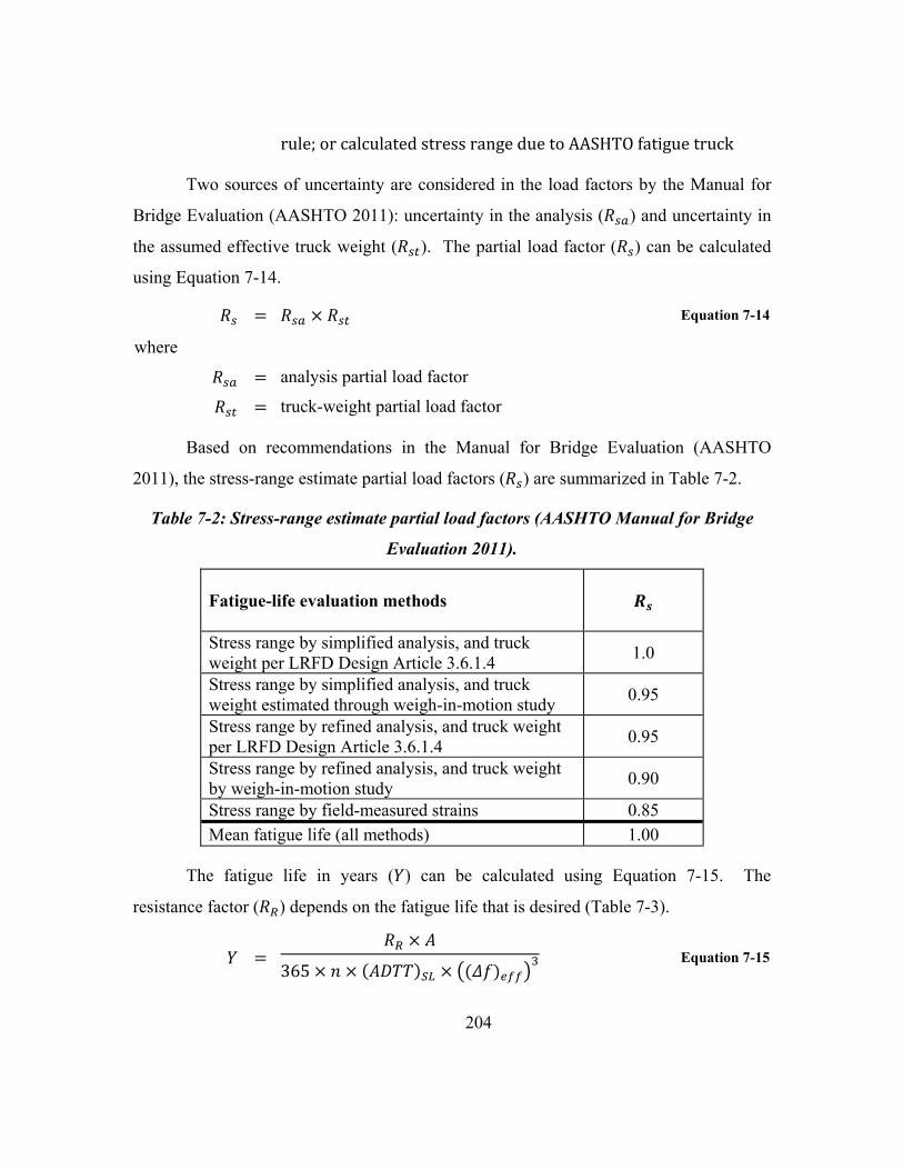
204

rule;orcalculatedstressrangeduetoAASHTOfatiguetruck

Two sources of uncertainty are considered in the load factors by the Manual for

Bridge Evaluation (AASHTO 2011): uncertainty in the analysis ( ) and uncertainty in

the assumed effective truck weight ( ). The partial load factor ( ) can be calculated

using Equation 7-14.

Equation 7-14

where

analysis partial load factor

truck-weight partial load factor

Based on recommendations in the Manual for Bridge Evaluation (AASHTO

2011), the stress-range estimate partial load factors ( ) are summarized in Table 7-2.

Table 7-2: Stress-range estimate partial load factors (AASHTO Manual for Bridge

Evaluation 2011).

Fatigue-life evaluation methods

Stress range by simplified analysis, and truck weight per LRFD Design Article 3.6.1.4

1.0

Stress range by simplified analysis, and truck weight estimated through weigh-in-motion study

0.95

Stress range by refined analysis, and truck weight per LRFD Design Article 3.6.1.4

0.95

Stress range by refined analysis, and truck weight by weigh-in-motion study

0.90

Stress range by field-measured strains 0.85

Mean fatigue life (all methods) 1.00

The fatigue life in years ( ) can be calculated using Equation 7-15. The

resistance factor ( ) depends on the fatigue life that is desired (Table 7-3).

365

Equation 7-15

205

where

resistance factor

numberofstress‐rangecyclespertruckpassage

averagenumberoftrucksperdayinasinglelaneaveragedoverthefatiguelife

The average number of trucks per day in a single lane averaged over the fatigue

life ( ) must be calculated to use Equation 7-15. The AASHTO approach

provides a graph in the commentary that can be used to estimate the average lifetime

traffic volume based on growth rates of 2%, 4%, 6%, and 8%. The number of stress-

range cycles ( ) can be estimated through LRFD Design Table 6.6.1.2.5-2 (AASHTO

LRFD Specifications 2010), influence lines, or field measurements.

Table 7-3: Resistance factor ( ) for evaluation, minimum, and mean fatigue life

(AASHTO Manual for Bridge Evaluation 2011).

AASHTO Fatigue

Category

Minimum

life Evaluation

life Mean

life A 1.0 1.7 2.8 B 1.0 1.4 2.0 Bʹ 1.0 1.5 2.4 C 1.0 1.2 1.3 Cʹ 1.0 1.2 1.3 D 1.0 1.3 1.6 E 1.0 1.3 1.6 Eʹ 1.0 1.6 2.5

The provisions in the AASHTO approach were evaluated by the researchers from

NCHRP Project 12-81 (Bowman, et al. 2012). A slightly different equation was

suggested (Equation 7-16). As can be seen, Equation 7-16 follows the same form as

Equation 7-11 (deterministic approach), except with load factors specified by AASHTO.

206

log

1

3651

log 1

Equation 7-16

where

estimated annual traffic-volume growth rate in percentage

presentageofconnectioninyears

averagenumberoftrucksperdayinyear

In NCHRP Project 12-81, the resistance factors were re-evaluated and updated.

There are also four levels to evaluate the fatigue life: minimum, evaluation 1, evaluation

2, and mean, which correspond to the respective probabilities of failure of 5%, 16%,

33%, and 50%.

Table 7-4: Resistance factor ( ) for evaluation, minimum, and mean fatigue life

(Bowman, et al. 2012).

AASHTO Fatigue

Category

Minimum

life Evaluation 1

life Evaluation 2

life Mean

life A 1.0 1.5 2.2 2.9 B 1.0 1.3 1.7 2.0 Bʹ 1.0 1.3 1.6 1.9 C 1.0 1.3 1.7 2.1 Cʹ 1.0 1.3 1.7 2.1 D 1.0 1.3 1.7 2.0 E 1.0 1.2 1.4 1.6 Eʹ 1.0 1.3 1.6 1.9

7.4 PROBABILISTIC APPROACH FOR CALCULATING THE REMAINING FATIGUE LIFE

Due to the uncertainty in calculating the fatigue life, reliability equations may be a

more appropriate calculation method. To solve for the remaining fatigue life using a

probabilistic approach, a fatigue limit state function ( ) must be considered. As

discussed in Section 2.3.3.3, the fatigue limit state function simplifies to Equation 7-17.

207

Because the function involves products, the limit state function can be modeled by a

lognormal distribution function (Equation 7-18).

0 Equation 7-17

ln ln 1 0 Equation 7-18

where

uncertaintymodelforthefatiguelimitstatefunction

Δ Palmgren‐Miner’scriticaldamageindex resistance

numberofaccumulatedcyclesatbridgeinyear correspondingtoastressrange loading

Lognormal distributions can be used for each random variable ( , , , and

) in Equation 7-17. As discussed in previous chapters, the fatigue damage is

characterized by both the stress range ( ) and number of stress cycles ( ). As such,

the two random variables can be combined into a single variable ( ) using Equation

7-19. Equation 7-19 can be substituted into Equation 7-17 and lognormal distributions

can be used to define the three variables ( , , and )).

Equation 7-19

where

total accumulated fatigue damage at time

A random variable is defined for to account for the uncertainty from using

Palmgren-Miner’s rule. As discussed in Section 2.2.1.1, Δ can be modeled by a

lognormal distribution with a median value ( ) of 1.0 and coefficient of variation ( ) of

30% (Wirsching 1984). For most tests, the median is 1.0 and the coefficient of variation

ranges between 30-60% (Wirsching and Chen 1988). When developing a procedure for

estimating the remaining fatigue life in bridges, Moses, Schilling, and Raju (1987) used a

value of of 15%. For this dissertation, = 1.0 and = 0.3 was assumed. The

lognormal parameters can be calculated using Equation 7-20 and Equation 7-21 (Table

7-5).

208

ln Equation 7-20

ln 1 Equation 7-21

where

median value of

coefficientofvariationof

Table 7-5: Lognormal parameters for random variable ( ) used in this dissertation.

Parameter Value 0.0 0.163

The variation in the fatigue constant ( ) can be determined from the test results in

the AASHTO fatigue database. After studying the data from 374 tests, Fisher et al.

(1970) concluded that log can be assumed to follow a normal distribution. As

such, log ) can also be assumed to follow a normal distribution, while follows a

lognormal distribution. To model using a lognormal distribution, the variation in

log ) must be transformed using Equation 7-22 and Equation 7-23. The derived

parameters of the lognormal distribution for each fatigue category are summarized in

Table 7-6.

ln 10 log Equation 7-22

ln 10 log Equation 7-23

where

mean parameter of lognormal function for fatigue constant ( )

deviation parameter of lognormal function for fatigue constant ( )

mean of fatigue constant ( )

normalizedstandard deviationoffatigueconstant

While random variables are used to describe and , the cumulative damage can

be estimated from measurements. Most measurement periods used to monitor highway

209

bridges tend to vary between two to eight weeks during year after the bridge was first

put in service. To calculate the cumulative fatigue damage, the previous amount of

damage has to be estimated. Assuming the average traffic volume grows geometrically at

a constant rate each year, the cumulative fatigue damage can be estimated by Equation

7-24. If a different traffic model is desired (i.e. one that limits the growth), it can be

substituted into the right side of Equation 7-24 because the total damage has to be

calculated each year.

1 1

Equation 7-24

where

mean damage in first year of service

yearevaluated

Table 7-6: Variation in fatigue constant ( ) from AASHTO Manual for Bridge

Evaluation (2011) and derived parameters for lognormal distribution.

AASHTO Fatigue

Category

Fatigue constant

Parameters for lognormal distribution

(code value) (mean value)

A 250×108 719×108 1.64 25.0 0.49 B 120×108 237×108 1.38 23.9 0.32 Bʹ 61×108 117×108 1.35 23.2 0.30 C 44×108 93×108 1.42 23.0 0.35 Cʹ 44×108 93×108 1.42 23.0 0.35 D 22×108 44×108 1.38 22.2 0.33 E 11×108 17×108 1.25 21.3 0.22 Eʹ 3.9×108 7.5×108 1.35 20.4 0.30

As seen from Equation 7-24, the cumulative damage depends on the mean

damage in the first year of service. The mean fatigue damage from the current year ( )

of service, obtained from measurements, can be used to approximate the damage from the

first year by using Equation 7-25.

210

1 Equation 7-25

where

mean damage in year

currentyear

Because and are lognormally distributed and the limit state function

(Equation 7-18) involves products, the reliability factor ( ) can be determined using

Equation 7-26.

Equation 7-26

where

parameterforthelognormaldistributionfor

ln2


ln 1

The probability of failure can be calculated using Equation 7-27.

Φ Equation 7-27

If there is no variability in the fatigue damage, the reliability index ( ) can be

simplified (Equation 7-28).

ln

Equation 7-28

If the index stress range and number of cycles at the index stress range are used,

rather than the fatigue damage, the reliability index can be calculated using Equation

7-29. Because the value used for the index stress range is selected by the engineer, the

211

number exhibits no variability. As such, all of the variability in fatigue damage would be

in the cumulative number of cycles for the bridge at the index stress range ( ).

Similarly, the mean number of cycles in the first year of service ( ) can be

calculated using Equation 7-30.

3 ln

Equation 7-29

1 Equation 7-30

where


ln2


ln 1

7.5 CALCULATING THE REMAINING FATIGUE LIFE AT BRIDGES MONITORED DURING

THIS INVESTIGATION

The remaining fatigue life of the four bridges monitored as part of the bridge can

be estimated using the equations listed in the previous sections. The amount of damage

was determined from both structural analysis and field monitoring. The fatigue lives

from both approaches are compared to evaluate the effectiveness of each source.

Because at least four weeks of data were not captured at Bridges C and D, the remaining

fatigue lives were not calculated for connection details at those bridges. In addition,

those two bridges have redundant structural systems and are not as critical as fracture-

critical bridges.

212

7.5.1 Bridge A

The effective stress range from structural analysis (Chapter 4) and the maximum-

measured stress range from field monitoring (Chapter 5) were larger than the CAFL.

Therefore, Bridge A is expected to have a finite fatigue life. The field-measured data

were used to calculate the fatigue life using all three methods. In contrast, only the

AASHTO approach was used to estimate the fatigue life using the results of structural

analysis. Two strain gages at Bridge A will be discussed in this section to exemplify the

methods for calculating the remaining fatigue life. Gage W-34s-TE was installed on the

east side of the top flange of the west longitudinal girder near the connection to floor

beam 34, whereas gage E-34s-TW was installed on the west side of the top flange of the

east longitudinal girder near the connection to floor beam 34. In this section, W-34s-TE

and E-34s-TW are referred to as the gages on the east and west girders, respectively

7.5.1.1 Deterministic Method

The fatigue life can be estimated from the deterministic method from the fatigue

damage for a given year and the annual rate of growth of traffic volume. If the annual

traffic growth rate is not known, the range of typical growth rates (2%-6%) can be

assumed to establish the bounds of the fatigue life. As more data are collected, the actual

growth rate could be extracted from traffic count data and used to improve the estimate.

To evaluate the remaining fatigue life, the damage in year 1 was estimated using

Equation 7-8. As seen in Table 7-7, there is considerable difference in the amount of

damage calculated in the first year of service for assumed rates of traffic growth between

2% and 6%. For both gage locations, the extrapolated fatigue damage in the first year for

an assumed annual growth rate of 2% is four times larger than the damage for an annual

growth rate of 6%.

213

Table 7-7: Fatigue damage in year 37 and extrapolated damage in year 1 for annual

growth rates of 2%, 4%, and 6%.

Annual growth


, . in year 1

, . in year 37

, . in year 1

, . in year 37

2% 610 1,250 2,990 6,070 4% 300 1,250 1,480 6,070 6% 150 1,250 750 6,070

The fatigue lives were calculated for the west and east girders (Table 7-8). The

age of the bridge connection was 37 years at the time of the calculation. As seen in Table

7-8, the design and mean fatigue lives have both been exceeded in the east girder, which

corresponds to a negative fatigue life. The mean fatigue life in the east girder has been

far exceeded if the 2% annual growth rate is correct. If the 6% growth rate is more

representative of traffic growth, the mean fatigue life has still been exceeded, but not by

as many years. .

Table 7-8: Calculated fatigue life in years for the west and east girders using the

deterministic approach.


2% 4% 6% 2% 4% 6%

5% (design) 37 43 45 10 16 22 50% (mean) 50 52 52 15 22 27

Based on the calculations, the west girder has a longer fatigue life than the east

girder. The design fatigue life of the west girder has only been exceeded for 2% annual

growth. For the other two growth rates, the fatigue life has not been exceeded for the

design and mean calculation levels.

7.5.1.2 AASHTO Method

Following the AASHTO method, the fatigue life can be calculated if the lifetime

average number of daily trucks crossing the bridge on a daily basis is known for the

214

calculated effective stress range. The effective stress range can be calculated by either

structural analysis or from field measurements. To provide a consistent level of

reliability for the different calculation levels, AASHTO recommends different partial

load factors depending on the method used to determine the effective stress range (Table

7-2).

The structural analysis of Bridge A was discussed in Section 4.1.5. The effective

stress range calculated for an AASHTO fatigue truck (54 kips) was 16 ksi in the east

girder. In 2005, the ADTT was determined to be 4,000. If 80% of the trucks are

assumed to cross the bridge in the right lane (suggested value in the AASHTO LRFD

Specifications (2010)), the fatigue life would have been exceeded in less than one year

for all calculation levels.

The fatigue life was severely underestimated using the results from the structural

analysis due to the assumptions of the model and because no knowledge of the weight of

typical truck traffic at Bridge A was known. As was discussed in Section 6.5, the stress

range for 4,000 cycles per day corresponds to an effective stress range of 5.15 ksi at floor

beam 34. Thus, the effective stress range from field monitoring was much less than the

effective stress range calculated from structural analysis using an AASHTO fatigue truck

at this bridge.

The fatigue damage obtained from field measurements can also be used with the

AASHTO method. Because the proposed method for calculating annual growth from

NCHRP project 12-81 provides an equivalent method to AASHTO Manual for Bridge

Evaluation (2011), Equation 7-16 was used to calculate the fatigue life.

A partial load factor of 0.85 is recommended for minimum, evaluation 1, and

evaluation 2 calculation levels when field measurements are used to calculate the fatigue

life. However, for the mean calculation level, the recommended value for the partial load

factor is 1.0. Because there is not much difference between the resistance factors ( ) for

the four levels of a Category E detail, the calculated fatigue lives at the minimum,

evaluation 1, and evaluation 2 levels are greater than the mean fatigue lives due to the

215

difference in the partial load factor (Table 7-9). This is unexpected result because the

mean fatigue life has a higher probability of failure than the other three calculation levels.

Table 7-9: Calculated fatigue life in years for different considerations using the

AASHTO approach for the west and east girders.


2% 4% 6% 2% 4% 6%

5% (design) 51 53 53 16 23 29 16% (evaluation 1) 57 57 56 18 26 31 33% (evaluation 2) 63 61 59 21 28 34

50% (mean) 51 53 53 15 23 29

7.5.1.3 Probabilistic Method

The probability of failure for a given year can be calculated using the probabilistic

approach. The approach allows a bridge owner to evaluate the risk of keeping a bridge in

service for a given duration and probability of failure. The fatigue life from the

probability of failure can be compared to other methods by determining the year when a

given level (i.e. 5%, 50%, etc.) is crossed. Unlike the other two methods, the

probabilistic method considers uncertainty in the fatigue damage. For Bridge A, the

uncertainty in the fatigue damage in year 37 is summarized in Table 7-10.

Table 7-10: Mean and standard deviation in year 37 for the west and east girders.

, . in year 37 , . in year 37

West girder 1,250 113 East girder 6,090 526

The probabilistic approach was applied to the west and east girders (Figure 7-3).

Comparing the two locations, the east girder has a higher probability of failure than the

west girder for any given year. This is expected since more damage occurred in the east

girder than the west girder during the monitoring period.

216

Because the annual rate of growth is not known for the bridge, a range of growth

rates (2%-6%) were considered. If the 2% model of annual growth is correct, the

probability of failure for the current age of the bridge is nearly 100% for the east girder.

If 6% growth is correct, the probability of failure is 95%.

Figure 7-3: Probability of failure in the (a) west and (b) east girders.

For the west girder, the probability of failure is between 0.5% and 11% in year 37.

As was discussed with Figure 7-2, 2% growth will have a higher probability of failure for

years prior to the current age of the bridge and slightly into the future. Though, in year

55 and beyond that point, 6% growth has a greater probability of failure as the

accumulated cycles for 6% growth exceed 2% growth.

7.5.1.4 Comparison

The calculated fatigue lives for different probability levels are considered in Table

7-11 for the three methods discussed (deterministic, AASHTO, and probabilistic).

Whereas the probability of failure for any given year can be determined using the

probabilistic approach, only certain probability levels can be determined using the

AASHTO (5%, 16%, 33%, and 50%) and deterministic approaches (5% and 50%).

0 10 20 30 40 50 60 70

Age of Bridge

0.01

0.10

1.00

0 10 20 30 40 50 60 70

Pro

bab

ilit

y o

f fa

ilu

re

Age of Bridge

6% growth

4% growth2% growth

Current age

= 5%

Mean life

Current age

Mean life

2% growth

6% growth

4% growth

(a) (b)

= 5%

217

Table 7-11: Calculated fatigue life in years for AASHTO, Deterministic, and

Probabilistic approaches for the west and east girders.


Deterministic AASHTO Probabilistic Deterministic AASHTO Probabilistic

2% annual growth 5% 37 51 33 10 16 9 16% - 57 39 - 18 11 33% - 63 45 - 20 13 50% 50 51 50 15 15 15

4% annual growth 5% 43 53 39 16 23 14 16% - 57 44 - 26 17 33% - 61 49 - 28 20 50% 52 52 52 22 23 22

6% annual growth 5% 45 53 42 22 29 20 16% - 56 46 - 31 23 33% - 59 50 - 34 26 50% 52 53 53 27 27 28

The deterministic and probabilistic approaches produced comparative fatigue

lives for the two probability levels for all growth rates. The fatigue lives in the east

girder were closer between the deterministic and probabilistic approaches because the

uncertainty in the current level of fatigue damage did not have as large of an influence on

the calculation of fatigue life. In contrast, the uncertainty had more of an influence on the

fatigue life for the west girder, which is why the fatigue life for the probabilistic method

had a lower fatigue life than the deterministic approach, in general.

The AASHTO approach was only comparative to the deterministic and

probabilistic approaches at a probability of failure of 50%. For the other three levels

(5%, 16%, and 33%), the fatigue life for the AASHTO method was much higher than the

probabilistic method. This can be attributed in part to the use of the partial load factor of

0.85.

218

7.5.2 Bridge B

From the measurement data, all of the stress ranges were below the CAFL. Thus,

the bridge is considered to have an infinite fatigue life. For the structural analysis

considered in Section 4.2.3, the largest effective stress range that was calculated was 4

ksi. Therefore, if the structural analysis data were used, the bridge would still be

considered to have an infinite life.

7.6 SUMMARY

The fatigue life of a particular bridge depends on the inherent variability of the

fatigue response of the bridge details, accumulation of fatigue cycles, and method of

calculation. Three methods of calculating the remaining fatigue life of a connection were

considered in this chapter. The output of the deterministic and AASHTO approaches is

the bridge age when the fatigue life is exceeded (for a specific probability of failure). For

the probabilistic method, the probability of failure for a given year is estimated.

The remaining fatigue lives of Bridges A and B were calculated using the three

methods discussed in this chapter. Based on the measured maxima at each bridge, Bridge

A was expected to have a finite fatigue life and Bridge B was expected to have an infinite

fatigue life. For Bridge A, the calculated fatigue lives based on the results of the

structural analysis was overly conservative and not representative of the actual behavior

of the connection. In contrast, the calculated fatigue lives corresponding to the measured

data were more representative than using structural analysis.

At Bridge A, the deterministic and probabilistic approaches produced comparative

fatigue lives at the two calculation levels (design and mean fatigue lives). The AASHTO

approach was only comparable to the deterministic and probabilistic approaches at the

mean fatigue life. At the other three calculation levels (design, evaluation 1, and

evaluation 2), the calculated fatigue life for the AASHTO approach was greater due to

the partial load factor of 0.85, which is allowed for field measurements.

219

CHAPTER 8

Conclusions

This chapter summarizes the conclusions of the research that was conducted as a

part of the NIST-funded project entitled, “Development of Rapid, Reliable and Economic

Methods for Inspection and Monitoring of Highway Bridges.” The research presented in

this dissertation represents a small portion of the research project as a whole. The major

conclusions from this dissertation will be discussed, as well as recommendations for field

monitoring.

8.1 SUMMARY

Highway bridges provide vital links in the transportation network, supplying

routes for daily commutes and the infrastructure needed to supply goods and services. As

such, transportation officials seek to maintain the bridge inventory under the pressure of

reduced budgets and an aging infrastructure. One of the critical types of structural

deterioration for steel bridges is fatigue-induced fracture.

If fracture is allowed to occur, localized damage can propagate to member failure

or even bridge collapse. As more bridges near or exceed their intended design lives,

transportation officials must make decisions on which bridges can be safely kept in

service and which need to be replaced or retrofitted. The primary method used to identify

structural deterioration is hands-on visual inspections. The inspections provide

transportation officials with qualitative data related to the number of cracks and rate of

crack growth, but quantitative data are often needed to distinguish among the bridges in

an inventory.

Recent legislation in the US Congress highlights the need for quantitative data to

identify the most vulnerable bridges. MAP-21, the Moving Ahead for Program in the 21st

Century Act, was signed into law on July 6, 2012 (Federal Highway Administration

220

2012). MAP-21 allows federal money to be used for new construction or rehabilitation

of highway bridges based on performance-based or risk-based criteria.

Calculating the remaining fatigue life is one means of providing quantitative data

to transportation officials. To estimate the remaining fatigue life of a bridge, the fatigue

damage must be characterized using either the results of structural analysis or measured

strains. Field monitoring provides a direct measure of the spectrum of stress ranges at the

location of a strain gage, whereas values for the representative fatigue truck, live load

distribution factors among girders, and dynamic impact factor must be assumed to

calculate the stress range using structural analysis.

With field-monitored data, the variable-amplitude stress ranges induced by trucks

of varying weights must be analyzed with a cycle-counting algorithm to produce a

histogram of stress ranges. The distribution of stress ranges is often converted to an

equivalent, constant stress range that can be used with the fatigue database (AASHTO S-

N curves). Historically, this conversion has been accomplished by calculating an

effective stress range using Palmgren-Miner’s linear damage rule. However, a new

method, the index stress range, of normalizing the damage was developed so that

different gage locations could be compared directly using the number of cycles as the

metric of damage accumulation (Chapter 3). Further techniques for visualizing the

contribution to damage and cumulative damage were presented to evaluate the influence

of a given stress range to the total amount of damage.

Once the accumulated fatigue damage has been estimated using the measured

data, the remaining fatigue life can be calculated. The fatigue life of a particular bridge

depends on the inherent variability of the fatigue response of the connection details, the

rate of accumulation of fatigue cycles (past, current, and future), and the method of

calculation. Deterministic approaches do not directly include uncertainty in the analysis,

yet using those approaches, the remaining fatigue life is easy to calculate and understand.

In contrast, probabilistic approaches provide a method for including many types of

uncertainty in the analysis, but the results are not as easily understood.

221

8.2 CONCLUSIONS

The focus of this dissertation was to develop methodologies that enable

transportation officials and/or engineers to collect quantitative information on fatigue

behavior of steel bridges by monitoring the service-load response. As such, techniques

for analyzing fatigue damage were developed and were applied to four steel bridges. The

inherent variability in fatigue damage was also evaluated on hourly, daily, and monthly

bases. The remaining fatigue lives of the bridges were calculated using both

deterministic and probabilistic approaches.

The conclusions from this dissertation are divided into three areas: techniques for

fatigue analysis, field monitoring, and calculating the remaining fatigue life. Conclusions

from each area are summarized in the following sections.

8.2.1 Techniques for Fatigue Analysis

Five techniques for analyzing fatigue damage from measured strain data were

discussed in Chapter 3. The first step in analyzing the fatigue damage is to use a cycle-

counting algorithm, such as the simplified rainflow algorithm, to transform a stress

history into a spectrum of stress ranges. Next, the total accumulation of fatigue damage

during a monitoring period can be expressed using the traditional approach—the effective

stress range—or a new approach—the index stress range. Finally, visualization

techniques, contribution to damage and cumulative damage, can be used to evaluate

whether lower or higher stress ranges are contributing significantly to the accumulation

of damage during the monitoring period.

1. The simplified rainflow method is well suited for fatigue analyses. As discussed

in the literature review, the simplified rainflow method is considered superior to

other cycle-counting methods because it identifies stress ranges associated with

closed-loop hystereses. By counting stress ranges in that manner, the histogram

of stress ranges is compatible with the empirical data from constant-amplitude

fatigue tests (Swenson and Frank 1984).

222

2. An index stress range is a better indicator of damage than an effective stress

range. Fatigue damage is characterized by the number of loading cycles applied

and the stress range. Because Palmgren-Miner’s rule was used to calculate the

fatigue damage, the total fatigue damage calculated using the effective stress

range is equivalent to that calculated using the index stress range. However, the

calculation of the effective stress range is sensitive to the number of cycles

measured by the data acquisition system. Thus, the effective stress range can

change drastically if the low-amplitude cycles are truncated from the calculation.

Because the data are normalized using the index stress range, the cycles

associated with the index stress range are not sensitive to truncating the small-

amplitude stress ranges. Therefore, the index stress range is a better indicator of

fatigue damage because it does not rely on the number of cycles measured.

3. The index stress range can be used to easily compare the measured response at

different locations of a bridge or of different bridges. By normalizing the data to

an index stress range, the number of cycles at the index stress range becomes the

direct metric of relative damage: twice as many cycles at the same index stress

range causes twice the damage. In contrast, the effective stress range and the

number of fatigue cycles at two locations will likely be different. Therefore, to

compare those locations using the effective stress range, the number of measured

cycles and cube of the effective stress range will have to be considered together to

compare the relative damage accumulation.

4. The contribution of each bin in a rainflow histogram to the fatigue damage and

cumulative damage can be calculated. As was noted in the literature review,

many researchers truncate the lower bins of the measured strain response under

the assumption that the lower stress ranges do not contribute to the fatigue

damage. There is not international agreement on how cycles below the constant-

amplitude fatigue life (CAFL) contribute to the fatigue damage. In the US, all

cycles are weighted equally (Palmgren-Miner’s rule). In Europe, stress cycles

less than the CAFL are weighed differently (different slope) than cycles above the

223

CAFL. Though studying how to handle cycles below the CAFL was not

explicitly addressed in this dissertation, the contribution to damage and

cumulative damage techniques allow an engineer to assess the influence of all

stress ranges, below and above the CAFL.

8.2.2 Field Monitoring

Strain data from four bridges were obtained and evaluated with respect to the

accumulation of fatigue damage. Two of the bridges featured twin girders and were

considered to be fracture critical, whereas the other two bridges had redundant structural

systems. The following are conclusions relative to the field monitoring of the four

bridges.

1. Fatigue damage obtained from field-monitored data is more representative than

damage calculated from structural analysis and standard design assumptions.

AASHTO LRFD Specifications (2010) recommends values to calculate the

fatigue damage using structural analysis, such as a representative fatigue truck

(Figure 2-16), dynamic impact factor (10% to 30%), and live load distribution

factors. However, those values may not be appropriate for all bridges and could

lead to significant error in the calculated remaining fatigue life. The use of

stresses calculated from measured strains provide representative data regarding

the number and amplitude of fatigue cycles during the measurement period,

thereby improving the estimate of the fatigue damage. For Bridge A, the

distribution factor, dynamic impact factor, and distribution of stress ranges that

were measured using strain gages were different than the values obtained

following AASHTO LRFD Specifications (2010). As such, the calculated

remaining fatigue life based on structural analysis was very conservative as

compared to the calculated remaining fatigue life based on strain gages.

2. Field-monitored data should be captured in weekly intervals due to hourly and

daily variations in fatigue damage. With each bridge, the traffic patterns varied

depending on the hour of the day and day of the week. On average, most fatigue

224

damage was induced between 8:00 AM and 6:00 PM, which corresponds to a

typical work day. For a given six-hour period, the maximum damage depended

on the bridge, but was either from 6:00 AM to 12:00 PM or 12:00 PM to 6:00

PM. On a daily basis, the maximum amount of damage occurred on weekdays,

rather than weekends. Due to such wide variation, the minimum amount of data

collected to calculate the fatigue damage should be a continuous week.

Monitoring for only part of the day or week will not be representative of the

average daily damage at the bridge.

3. One continuous week of data is typically inadequate for long-term projections

of fatigue damage. Traffic patterns are irregular and can increase or decrease due

to weather, accidents, and many other factors. As such, obtaining only a

continuous week of data is inadequate for long-term projections of fatigue

damage. For Bridge A, the amount of induced fatigue damage also varied month

to month. The estimate in the average amount of fatigue damage can be improved

by monitoring over longer periods of time. Four weeks is considered to be the

minimum monitoring period to make long-term projections.

4. Most of the fatigue damage is caused by a narrow range of stress ranges, which

corresponds to typical truck traffic. From the cumulative-damage plots for each

bridge, 95% of the fatigue damage was typically induced by less than 50% of the

range of stress cycles. Those cycles correspond to vehicles that cause a mid-level

amount of stress a moderate number of times per day (typical truck traffic).

Though there are many more cycles at the lower stress ranges, those cycles did

not cause a significant amount of damage due to the low value of stress. If the

cycles corresponding to electromechanical noise from the data acquisition system

were not truncated from the rainflow histograms (Bridges B and C), then the

contribution to damage at the lower stress ranges was very large. However, those

cycles should be truncated because the electromechanical noise does not

correspond to load-induced fatigue cycles and causes no fatigue damage. The

225

largest stress ranges from heavier vehicles also did not cause a significant amount

of damage because they occurred with low frequency.

5. The benefit of retrofitting Bridge A could be tracked effectively using an index

stress range. Each phase in the construction of the retrofit (right lane closed, left

lane closed, both lanes reopened) could be identified from the daily fatigue

damage because the data was normalized using an index stress range. In addition,

the impact of the retrofit could be quantified before and after the construction.

The significant reduction in the fatigue damage in the top flange and moderate

reduction in the bottom flange is consistent with composite action between the

concrete deck and longitudinal girders. The retrofit was not specifically designed

to create composite action and could degrade with time. The gages at the detail

could continue to be monitored to detect if the composite action degrades.

6. Crack propagation gages can be used to track crack growth on steel bridges.

By measuring the resistance of the gage every 30 minutes, the drift of the gage

due to temperature was less than the change in resistance due to a wire break.

Thus, the gage can be used to track crack growth between bridge inspections and

notify transportation officials if problems arise.

8.2.3 Remaining Fatigue Life

After the fatigue damage had been determined and characterized, the remaining

fatigue lives of the bridges were calculated using both deterministic and probabilistic

approaches. The following are conclusions relative to the calculation of the remaining

fatigue life that was discussed in Chapter 7.

1. There is much uncertainty in estimating the fatigue life of a bridge. Traffic

patterns can change drastically from hour to hour, day to day, and year to year.

Weather, traffic accidents, and many other sources affect the accumulation of

traffic and fatigue damage at a bridge. Where possible, historic traffic counts or

strain data should be utilized to validate the growth model chosen for a particular

bridge.

226

2. Deterministic and probabilistic methods can provide similar remaining fatigue

lives for some probabilities of failure. If the uncertainty from determining the

fatigue damage is small (as for Bridge A), deterministic and probabilistic methods

can provide comparable results. Though, using a deterministic approach, the

calculated fatigue life corresponds to a limited number of probabilities of failure

(5%, 16%, 33%, and 50%, depending on the method).

3. For the AASHTO approach (AASHTO Manual for Bridge Evaluation 2011),

reducing the stress range by a factor of 0.85 when field-monitored data are used

is not justified. With the new equation proposed by NCHRP Project 12-81, the

only difference between the deterministic method discussed in Section 7.2 and the

AASHTO approach is the stress-range estimate partial load factor ( ).

AASHTO allows a load factor of 0.85 when field-monitored data are used to

calculate the effective stress range. By reducing the stress range by 0.85, the

fatigue life increases, which is not justified with the other factors considered. In

addition, for certain fatigue categories, such as Category E, the mean fatigue life

will produce a smaller value than the other fatigue lives (minimum, evaluation 1,

and evaluation 2).

4. The probabilistic method provides the framework for calculating the risk of

keeping a bridge in service. Risk involves making decisions with the possibility

of loss. With the probability of failure calculated for each year, the owner can

weigh the potential cost from collapse or failure with the cost from replacing the

bridge. The loss can take into account user costs from the bridge being closed,

cost of bridge replacement, and cost of additional inspections. Knowing all of

these costs, the owner can determine the optimal point of replacing the bridge

and/or increasing the rate of inspections to minimize the loss to the public.

8.3 RECOMMENDATIONS

A variety of steps are needed to characterize the fatigue damage at a bridge and

estimate the remaining fatigue life through field monitoring. First, critical fatigue

227

connection details must be identified through a combination of engineering judgment and

analysis. Some poor fatigue details may not be immediately apparent and could be

discovered from inspection reports. Creating a structural-analysis model of the bridge

can be useful in determining locations with the highest stress range, as those locations

may not always correspond to the location with the highest moment (as in Bridge A).

Once the critical locations have been identified, durable strain gages should be

installed and coupled with a high-resolution data acquisition system. Wired or wireless

data acquisition systems may be used. Though, wireless systems offer many benefits,

such as lower costs, quicker installations, and less susceptibility to high-amplitude spikes

due to lightning strikes, the wireless systems also require more power than a comparable

number of channels on a wired system and are subject to loss of data from wireless

interference. Transportation officials and/or the engineer must weigh those benefits when

choosing a data acquisition system. Nonetheless, the following features are

recommended for the data acquisition system: electromechanical noise is limited to 1-5

microstrain at faster scan rates (50-100 scans per second); the sensors can be calibrated

using shunt calibration; and high-precision completion resistors should be utilized to

minimize drift from temperature fluctuations if quarter-bridge sensors are used.

If a long-term projection of the fatigue damage is desired, four weeks of data are

recommended. As mentioned previously, due to the hourly and daily variation in

damage, a continuous week of data is the minimum for determining the average daily

fatigue damage. If the data acquisition system is a permanent or semi-permanent

installation, multiple months of data can be captured continuously. Though, if power is a

concern, as it is with wireless data acquisition systems, two continuous weeks of data

could be captured in a particular month and two more continuous weeks of data could be

captured in another month. The data should not correspond to a week with a national

holiday, as that will lower the estimate of the fatigue damage.

The dynamic data should be analyzed using the techniques described in Chapter

3. The spectrum of stress ranges from typical traffic can be identified using the

simplified rainflow method. Care should be taken to choose parameters (size of bins and

228

number of bins) for the rainflow method such that wide-enough spectra of stress ranges

are selected. The calculated stress range from an AASHTO fatigue truck crossing the

bridge can be used as an estimate of the required spectrum of the stress ranges: the

spectrum should be at least twice as large as the calculated stress range. Though, the

histogram of stress ranges should be investigated after a few days of monitoring to ensure

that the spectrum is large enough.

The width of each rainflow bin is important. A width of 5 microstrain was used

for each bin in this dissertation, and it provided enough fidelity that the contribution to

damage and cumulative damage plots were smooth. Larger bin widths can be used to

limit the amount of data that needs to be transferred; but the plots may become more

jagged. In addition, the estimate of the fatigue damage might become less accurate

because all of the cycles in a bin are assumed to have the same stress range (Figure 8-1).

If a very wide bin width is used (i.e. 30 microstrain) and the majority of the cycles are

near the bottom of the bin (i.e. 0-5 microstrain), assuming all of the cycles were 15

microstrain would over-estimate the damage. At Bridge C, enlarging the width of the bin

size to 15 microstrain increased the fatigue damage by approximately 1%. Enlarging the

width of the bin size to 30 microstrain increased the fatigue damage by 10%. At Bridge

A, before the construction of the retrofit, increasing the width of the bins did not

significantly influence the fatigue damage. However, after the construction of the retrofit

at Bridge A, the fatigue damage increased by nearly 20% if a bin width of 30 microstrain

was used as compared to 5 microstrain. As such, a bin width between 5-15 microstrain is

recommended.

The time period of a rainflow analysis can also influence the results. If the length

is too long, a large, fictitious cycle due to the drift of the strain gage with temperature

could be counted. If the length is too short, then the count could be biased due to partial

cycles being counted as full cycles. A length of 30 min was chosen for all of the analyses

in this dissertation. In 30 min, the drift of the gage due to temperature will be minimal

and the time is long enough to provide a correct count.

229

Figure 8-1: Increase in fatigue damage ( , . ) due to change in width of the

rainflow bin.

Once the distribution of stress ranges has been determined, the amount of damage

can be calculated using an index stress range. In addition, the effect of each rainflow bin

can be evaluated using the contribution to damage and cumulative damage techniques to

validate that the lower (typically truncated due to electromechanical noise of the data

acquisition system) and higher cycles (often questioned whether the larger cycles are load

induced or due to spikes in the data acquisition system) do not cause significant damage.

The remaining fatigue life can then be calculated using one of the approaches discussed

in Chapter 7.

Because calculating the remaining fatigue life relies heavily on projecting past,

current, and future traffic volumes, a permanent or semi-permanent data acquisition

system should be considered, especially at bridges nearing their intended design life.

With fatigue data from multiple years, the amount of traffic growth can be estimated. In

the absence of fatigue data from strain gages, traffic-count data from transportation

officials can be used to estimate traffic growth.

0%

5%

10%

15%

20%

5 10 15 20 25 30Bin size (microstrain)

Bridge A (after retrofit)

Bridge A (before retrofit)

Bridge C

Incr

ease

in

230

APPENDIX A

Strain data from Bridge A (4/1/2011 to 5/1/2012)

The data from 4/1/2011 to 5/1/2012 for all strain gages at Bridge A are presented

in this Appendix. A summary of the fatigue damage prior to and after the construction of

the retrofit are presented in Table A-1 and Table A-2, respectively.

Table A-1: Summary of fatigue damage prior to the construction of the retrofit.

Gir

der

FB

Pos

itio

n

Fla

nge

Not

e

. , ksi , ksi , Number of

days monitored

, .

Gages installed on the east longitudinal girder

E 27 s TE 11.2 0.93 39,700 71 350

E 27 s TW 9.4 0.86 64,900 23 450

E 27 s BE 9.6 0.79 137,000 71 750

E 27 s BW 7.6 0.74 114,000 23 500

E 34 s TE 23.7 2.26 56,300 71 7,080

E 34 s TW 24.9 2.37 41,400 71 6,070

E 35 n TE 27.6 2.89 39,800 71 10,400

E 35 n TW 11.5 0.83 40,000 71 250

E 35 s TE 23.9 2.69 40,500 71 8,620

E 35 s TW 20.7 1.80 35,000 71 2,260

E 35 n BE 26.3 1.81 133,000 71 8,600

E 35 n BW 27.3 1.85 127,000 71 8,900

Gages installed on the west longitudinal girder

W 34 s TE 17.2 1.44 38,000 71 1,250

W 34 s TW 14.3 1.24 41,300 71 860

W 35 s TE 12.8 1.20 34,700 71 650

W 35 s TW 13.4 1.27 40,100 71 900

W 35 s BE 14.0 0.98 128,000 71 1,340

W 35 s BW 16.9 1.12 144,000 71 2,660

231

Table A-2: Summary of fatigue damage after the construction of the retrofit. G

ird

er

FB

Pos

itio

n

Fla

nge

Not

e


days monitored

, .


E 27 s TE 5.7 0.80 39,394 2 220

E 27 s TW 5.7 0.81 61,679 2 370

E 27 s BE 6.3 0.73 124,748 2 540

E 27 s BW 5.7 0.70 100,334 2 380

E 33 n TE 6.2 0.72 49,772 96 210

E 33 n TW 16.3 0.57 54,300 94 110

E 34 s TE P 2.4 0.32 16,507 96 6

E 34 s TW P 10.9* 0.29 18,884 96 5

E 34 s TE 9.9 1.00 97,518 96 1,060

E 34 s TW 10.2 1.02 83,740 98 980

E 34 BE 19.1 1.52 170,894 83 6,640

E 34 BW 19.6 1.54 164,297 96 6,520

E 35 n TE 5.0 0.61 60,050 98 150

E 35 n TW 6.0 0.58 70,432 96 150

E 35 s TE 3.6 0.42 46,217 98 40

E 35 s TW 3.3 0.45 43,021 96 40

E 35 n BE 18.6 1.45 170,960 98 5,760

E 35 n BW 19.2 1.47 165,975 98 5,810

Gages installed on the west longitudinal girder

W 34 s TE 29.1* 0.48 120,770 94 150

W 34 s TW 10.7 0.36 117,802 98 60

W 35 s TE 11.8* 0.20 46,809 96 4

W 35 s TW 8.9* 0.15 37,880 98 2

W 35 s BE 29.1* 0.82 175,458 98 1,050

W 35 s BW 15.6 0.96 192,092 98 1,860 *Value may be due to spikes in the data acquisition system. See details of gage.

232

Figure A-1: Response of bridge at gage E-35n-TE.

End support, typ.

0.001

0.01

0.1

1

10

100

1000

10000

100000

0 10 20 30

Ave

rage

nu

mb

er o

f cy

cle

s p

er

day

Stress range (ksi)

0.001

0.01

0.1

1

10

100

1000

10000

100000

0 10 20 30

Ave

rage

nu

mb

er o

f cy

cle

s p

er

day

Stress range (ksi)

0

0.2

0.4

0.6

0.8

1

0 10 20 30

Ave

rage

dai

ly

cum

ula

tive

dam

age

Stress range (ksi)

0

200

400

600



Interior support, typ.

30′-0″

FB 35Hanger


After construction

Prior to construction

Gage

(b) Histogram of stress ranges prior to construction (average of 71 days)

(c) Histogram of stress ranges after construction (average of 98 days)

(a) Location of gage (installed 2′-0″ north of FB 35)

After construction


Maximum

(d) Average daily contribution to effective fatigue damage

(e) Average daily cumulative damage

Co

ntr

ibu

tio

n t

o

233

Figure A-1 (cont’d): Response of bridge at gage E-35n-TE.

0

4,000

8,000

12,000

16,000

Date

0

100

200

300

400

Date

0

4,000

8,000

12,000

16,000

Date

Prior to constructionDuring

constructionAfter construction


After construction

(f) Daily fatigue damage ( ) for total monitoring period

(g) Daily fatigue damage ( ) for monitoring period prior to construction

(h) Daily fatigue damage ( ) for monitoring period after construction (different vertical scale than (f))

234

Figure A-2: Response of bridge at gage E-35n-TW.


0

0.2

0.4

0.6

0.8

1

0 10 20 30

Ave

rage

dai

ly

cum

ula

tive

dam

age

Stress range (ksi)

0

10

20

30

40

50



30′-0″

FB 35Hanger


After construction


Gage




After construction


Maximum

0.001

0.01

0.1

1

10

100

1000

10000

100000

0 10 20 30

Ave

rage

nu

mb

er o

f cy

cle

s p

er

day

Stress range (ksi)

0.001

0.01

0.1

1

10

100

1000

10000

100000

0 10 20 30

Ave

rage

nu

mb

er o

f cy

cle

s p

er

day

Stress range (ksi)

(e) Average daily cumulative damage(d) Average daily contribution to effective fatigue damage

Co

ntr

ibu

tio

n t

o

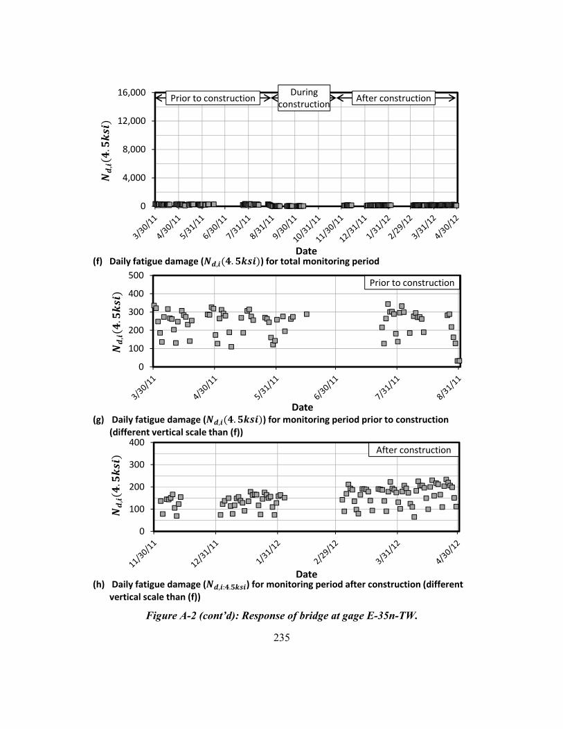
235

Figure A-2 (cont’d): Response of bridge at gage E-35n-TW.

(g) Daily fatigue damage ( ) for monitoring period prior to construction (different vertical scale than (f))

0

100

200

300

400

Date

0

100

200

300

400

500

Date

0

4,000

8,000

12,000

16,000

Date




After construction



236

Figure A-3: Response of bridge at gage E-35s-TE.


0

0.2

0.4

0.6

0.8

1

0 10 20 30

Ave

rage

dai

ly

cum

ula

tive

dam

age

Stress range (ksi)

0

100

200

300

400



30′-0″

FB 35Hanger


After construction




(a) Location of gage (installed 2′-0″ south of FB 35)

After construction


Maximum

0.001

0.01

0.1

1

10

100

1000

10000

100000

0 10 20 30

Ave

rage

nu

mb

er o

f cy

cle

s p

er

day

Stress range (ksi)

Gage

0.001

0.01

0.1

1

10

100

1000

10000

100000

0 10 20 30

Ave

rage

nu

mb

er o

f cy

cle

s p

er

day

Stress range (ksi)


Co

ntr

ibu

tio

n t

o

237

Figure A-3 (cont’d): Response of bridge at gage E-35s-TE.

0

20

40

60

80

100

Date

0

4,000

8,000

12,000

16,000

Date

0

4,000

8,000

12,000

16,000

Date




After construction




238

Figure A-4: Response of bridge at gage E-35s-TW.


0

0.2

0.4

0.6

0.8

1

0 10 20 30

Ave

rage

dai

ly

cum

ula

tive

dam

age

Stress range (ksi)

0

100

200

300

400



30′-0″

FB 35Hanger


After construction


Gage




After construction


Maximum

0.001

0.01

0.1

1

10

100

1000

10000

100000

0 10 20 30

Ave

rage

nu

mb

er o

f cy

cle

s p

er

day

Stress range (ksi)

0.001

0.01

0.1

1

10

100

1000

10000

100000

0 10 20 30

Ave

rage

nu

mb

er o

f cy

cle

s p

er

day

Stress range (ksi)


Co

ntr

ibu

tio

n t

o

239

Figure A-4 (cont’d): Response of bridge at gage E-35s-TW.

0

4,000

8,000

12,000

16,000

Date

0

1,000

2,000

3,000

4,000

Date

0

20

40

60

80

100

Date




After construction




240

Figure A-5: Response of bridge at gage E-35n-BE.


0

200

400

600


0

0.2

0.4

0.6

0.8

1

0 10 20 30

Ave

rage

dai

ly

cum

ula

tive

dam

age

Stress range (ksi)


30′-0″

FB 35Hanger


After construction





After construction


Maximum

0.001

0.01

0.1

1

10

100

1000

10000

100000

0 10 20 30

Ave

rage

nu

mb

er o

f cy

cle

s p

er

day

Stress range (ksi)

Gage

0.001

0.01

0.1

1

10

100

1000

10000

100000

0 10 20 30

Ave

rage

nu

mb

er o

f cy

cle

s p

er

day

Stress range (ksi)


Co

ntr

ibu

tio

n t

o

241

Figure A-5(cont’d): Response of bridge at gage E-35n-BE.

0

2,000

4,000

6,000

8,000

10,000

Date

0

4,000

8,000

12,000

16,000

Date

0

4,000

8,000

12,000

16,000

Date




After construction




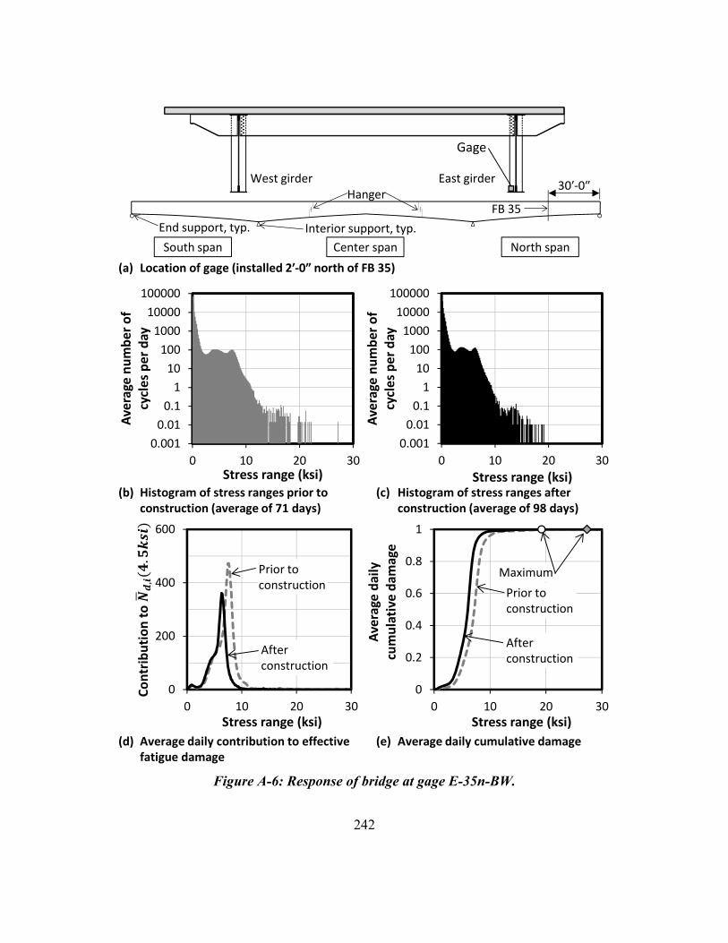
242

Figure A-6: Response of bridge at gage E-35n-BW.


0

0.2

0.4

0.6

0.8

1

0 10 20 30

Ave

rage

dai

ly

cum

ula

tive

dam

age

Stress range (ksi)

0

200

400

600



30′-0″

FB 35Hanger


After construction





After construction


Maximum

0.001

0.01

0.1

1

10

100

1000

10000

100000

0 10 20 30

Ave

rage

nu

mb

er o

f cy

cle

s p

er

day

Stress range (ksi)

Gage

0.001

0.01

0.1

1

10

100

1000

10000

100000

0 10 20 30

Ave

rage

nu

mb

er o

f cy

cle

s p

er

day

Stress range (ksi)


Co

ntr

ibu

tio

n t

o

243

Figure A-6 (cont’d): Response of bridge at gage E-35n-BW.

0

4,000

8,000

12,000

16,000

Date

0

4,000

8,000

12,000

16,000

Date

0

2,000

4,000

6,000

8,000

10,000

Date




After construction




244



0

100

200

300

400


0

0.2

0.4

0.6

0.8

1

0 10 20 30

Ave

rage

dai

ly

cum

ula

tive

dam

age

Stress range (ksi)


37′-6″

FB 34Hanger


After construction





After construction


Maximum

0.001

0.01

0.1

1

10

100

1000

10000

100000

0 10 20 30

Ave

rage

nu

mb

er o

f cy

cle

s p

er

day

Stress range (ksi)

Gage

0.001

0.01

0.1

1

10

100

1000

10000

100000

0 10 20 30

Ave

rage

nu

mb

er o

f cy

cle

s p

er

day

Stress range (ksi)


Co

ntr

ibu

tio

n t

o

245

Figure A-7 (cont’d): Response of bridge at gage E-34s-TE.

0

500

1,000

1,500

2,000

Date

0

3,000

6,000

9,000

12,000

Date

0

4,000

8,000

12,000

16,000

Date




After construction




246



0

0.2

0.4

0.6

0.8

1

0 10 20 30

Ave

rage

dai

ly

cum

ula

tive

dam

age

Stress range (ksi)

0

100

200

300

400



37′-6″

FB 34Hanger


After construction





After construction


Maximum

0.001

0.01

0.1

1

10

100

1000

10000

100000

0 10 20 30

Ave

rage

nu

mb

er o

f cy

cle

s p

er

day

Stress range (ksi)

0.001

0.01

0.1

1

10

100

1000

10000

100000

0 10 20 30

Ave

rage

nu

mb

er o

f cy

cle

s p

er

day

Stress range (ksi)

Gage


Co

ntr

ibu

tio

n t

o

247

Figure A-8 (cont’d): Response of bridge at gage E-34s-TW.

0

4,000

8,000

12,000

16,000

Date

0

2,000

4,000

6,000

8,000

10,000

Date

0

500

1,000

1,500

2,000

Date




After construction




248

Figure A-9: Response of bridge at gage W-35s-TE.


0

10

20

30

40

50


0

0.2

0.4

0.6

0.8

1

0 10 20 30

Ave

rage

dai

ly

cum

ula

tive

dam

age

Stress range (ksi)

0.001

0.01

0.1

1

10

100

1000

10000

100000

0 10 20 30

Ave

rage

nu

mb

er o

f cy

cle

s p

er

day

Stress range (ksi)

0.001

0.01

0.1

1

10

100

1000

10000

100000

0 10 20 30

Ave

rage

nu

mb

er o

f cy

cle

s p

er

day

Stress range (ksi)


30′-0″

FB 35Hanger


After construction


Gage




After construction


Maximum


Co

ntr

ibu

tio

n t

o

249

Figure A-9 (cont’d): Response of bridge at gage W-35s-TE.

0

10

20

30

40

50

Date

0

500

1,000

1,500

2,000

Date

0

4,000

8,000

12,000

16,000

g

Date




After construction




250

Figure A-10: Response of bridge at gage W-35s-TW.


0

0.2

0.4

0.6

0.8

1

0 10 20 30

Ave

rage

dai

ly

cum

ula

tive

dam

age

Stress range (ksi)

0

10

20

30

40

50


0.001

0.01

0.1

1

10

100

1000

10000

100000

0 10 20 30

Ave

rage

nu

mb

er o

f cy

cle

s p

er

day

Stress range (ksi)

0.001

0.01

0.1

1

10

100

1000

10000

100000

0 10 20 30

Ave

rage

nu

mb

er o

f cy

cle

s p

er

day

Stress range (ksi)


30′-0″

FB 35Hanger


After construction


Gage




After construction


Maximum


Co

ntr

ibu

tio

n t

o

251

Figure A-10 (cont’d): Response of bridge at gage W-35s-TW.

0

4,000

8,000

12,000

16,000

Date

0

500

1,000

1,500

2,000

2,500

Date

0

10

20

30

40

50

Date




After construction




252

Figure A-11: Response of bridge at gage W-35s-BE.


0

20

40

60

80

100


0

0.2

0.4

0.6

0.8

1

0 10 20 30

Ave

rage

dai

ly

cum

ula

tive

dam

age

Stress range (ksi)

0.001

0.01

0.1

1

10

100

1000

10000

100000

0 10 20 30

Ave

rage

nu

mb

er o

f cy

cle

s p

er

day

Stress range (ksi)

0.001

0.01

0.1

1

10

100

1000

10000

100000

0 10 20 30

Ave

rage

nu

mb

er o

f cy

cle

s p

er

day

Stress range (ksi)


30′-0″

FB 35Hanger


After construction


Gage




After construction


Maximum


Co

ntr

ibu

tio

n t

o

253

Figure A-11 (cont’d): Response of bridge at gage W-35s-BE.

0

500

1,000

1,500

2,000

2,500

3,000

Date

0

500

1,000

1,500

2,000

2,500

Date

0

4,000

8,000

12,000

16,000

Date




After construction




254

Figure A-12: Response of bridge at gage W-35s-BW.


0

0.2

0.4

0.6

0.8

1

0 10 20 30

Ave

rage

dai

ly

cum

ula

tive

dam

age

Stress range (ksi)

0

20

40

60

80

100


0.001

0.01

0.1

1

10

100

1000

10000

100000

0 10 20 30

Ave

rage

nu

mb

er o

f cy

cle

s p

er

day

Stress range (ksi)

0.001

0.01

0.1

1

10

100

1000

10000

100000

0 10 20 30

Ave

rage

nu

mb

er o

f cy

cle

s p

er

day

Stress range (ksi)


30′-0″

FB 35Hanger

East girder

After construction


Gage




After construction


Maximum

West girder


Co

ntr

ibu

tio

n t

o

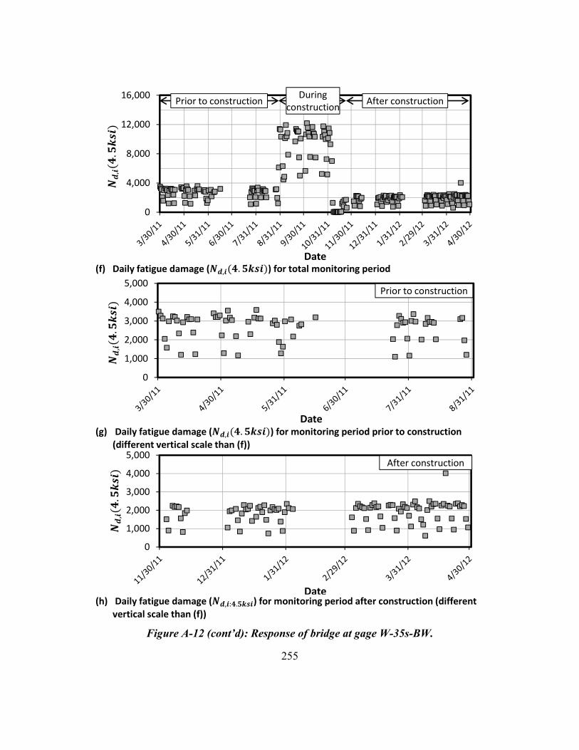
255

Figure A-12 (cont’d): Response of bridge at gage W-35s-BW.

0

4,000

8,000

12,000

16,000

Date

0

1,000

2,000

3,000

4,000

5,000

Date

0

1,000

2,000

3,000

4,000

5,000

Date




After construction




256

Figure A-13: Response of bridge at gage W-34s-TE.


0

10

20

30

40

50


0

0.2

0.4

0.6

0.8

1

0 10 20 30

Ave

rage

dai

ly

cum

ula

tive

dam

age

Stress range (ksi)

0.001

0.01

0.1

1

10

100

1000

10000

100000

0 10 20 30

Ave

rage

nu

mb

er o

f cy

cle

s p

er

day

Stress range (ksi)

0.001

0.01

0.1

1

10

100

1000

10000

100000

0 10 20 30

Ave

rage

nu

mb

er o

f cy

cle

s p

er

day

Stress range (ksi)


HangerWest girder East girder

After construction


Gage




After construction

Prior to construction Maximum

37′-6″

FB 34


Co

ntr

ibu

tio

n t

o

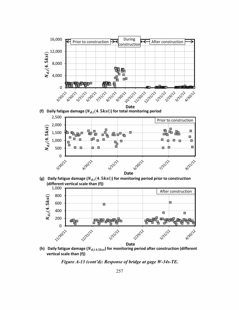
257

Figure A-13 (cont’d): Response of bridge at gage W-34s-TE.

0

200

400

600

800

1,000

Date

0

500

1,000

1,500

2,000

2,500

Date

0

4,000

8,000

12,000

16,000

Date




After construction




258

Figure A-14: Response of bridge at gage W-34s-TW.


0

0.2

0.4

0.6

0.8

1

0 10 20 30

Ave

rage

dai

ly

cum

ula

tive

dam

age

Stress range (ksi)

0

10

20

30

40

50


0.001

0.01

0.1

1

10

100

1000

10000

100000

0 10 20 30

Ave

rage

nu

mb

er o

f cy

cle

s p

er

day

Stress range (ksi)

0.001

0.01

0.1

1

10

100

1000

10000

100000

0 10 20 30

Ave

rage

nu

mb

er o

f cy

cle

s p

er

day

Stress range (ksi)



After construction





After construction

Prior to construction Maximum

37′-6″

FB 34

Gage


Co

ntr

ibu

tio

n t

o

259

Figure A-14 (cont’d): Response of bridge at gage W-34s-TW.

0

4,000

8,000

12,000

16,000

Date

0

500

1,000

1,500

2,000

Date

0

50

100

150

200

250

Date




After construction




260



0

10

20

30

40

50


0

200

400

600

800

g

Date




FB 27Hanger


Gage

(d) Daily fatigue damage ( ) for total monitoring period

0.001

0.01

0.1

1

10

100

1000

10000

100000

0 10 20 30

Ave

rage

nu

mb

er o

f cy

cles

pe

r d

ay

Stress range (ksi)



(c) Average daily contribution to effective fatigue damage

90′-0″


Co

ntr

ibu

tio

n t

o

261



0

200

400

600

800

Date


FB 27Hanger


Gage

0.001

0.01

0.1

1

10

100

1000

10000

100000

0 10 20 30

Ave

rage

nu

mb

er o

f cy

cles

pe

r d

ay

Stress range (ksi)

0

10

20

30

40

50






90′-0″




Co

ntr

ibu

tio

n t

o

262

Figure A-17: Response of bridge at gage E-27s-BE.


0

20

40

60

80

100


0

300

600

900

1,200

1,500

Date


FB 27Hanger


Gage

0.001

0.01

0.1

1

10

100

1000

10000

100000

0 10 20 30

Ave

rage

nu

mb

er o

f cy

cles

pe

r d

ay

Stress range (ksi)





90′-0″




Co

ntr

ibu

tio

n t

o

263

Figure A-18: Response of bridge at gage E-27s-BW.


0

300

600

900

1,200

1,500

Date

0

20

40

60

80

100



FB 27Hanger


Gage

0.001

0.01

0.1

1

10

100

1000

10000

100000

0 10 20 30

Ave

rage

nu

mb

er o

f cy

cles

pe

r d

ay

Stress range (ksi)





90′-0″




Co

ntr

ibu

tio

n t

o

264

Figure A-19: Response of bridge at gage E-34-BE.


0

100

200

300

400

500


0

2,000

4,000

6,000

8,000

10,000

Date

After construction


HangerWest girder

Gage

0.001

0.01

0.1

1

10

100

1000

10000

100000

0 10 20 30

Ave

rage

nu

mb

er o

f cy

cles

pe

r d

ay

Stress range (ksi)

After construction

(b) Histogram of stress ranges after construction (average of 83 days)


(a) Location of gage

37′-6″

FB 34

East girder

(d) Daily fatigue damage ( ) for monitoring period after construction

Co

ntr

ibu

tio

n t

o

265

Figure A-20: Response of bridge at gage E-34-BW.


0

100

200

300

400

500


0

2,000

4,000

6,000

8,000

10,000

Date



Gage

0.001

0.01

0.1

1

10

100

1000

10000

100000

0 10 20 30

Ave

rage

nu

mb

er o

f cy

cles

pe

r d

ay

Stress range (ksi)

After construction




37′-6″

FB 34

After construction


Co

ntr

ibu

tio

n t

o

266

Figure A-21: Response of bridge at gage E-34s-TE-P.


0

10

20

30

40

50

g

Date

0

2

4

6

8

10


After construction


HangerWest girder

0.001

0.01

0.1

1

10

100

1000

10000

100000

0 10 20 30

Ave

rage

nu

mb

er o

f cy

cles

pe

r d

ay

Stress range (ksi)

After construction


(a) Location of gage (installed 6″ south of FB 34 on cover plate from retrofit)


Gage

37′-6″

FB 34


Co

ntr

ibu

tio

n t

o

267

Figure A-22: Response of bridge at gage E-34s-TW-P.


0

10

20

30

40

50

g

Date

0

2

4

6

8

10



HangerWest girder

0.001

0.01

0.1

1

10

100

1000

10000

100000

0 10 20 30

Ave

rage

nu

mb

er o

f cy

cles

pe

r d

ay

Stress range (ksi)

After construction


(a) Location of gage (installed 6″ south of FB 34 on cover plate from retrofit)


Gage

37′-6″

FB 34

After construction


Co

ntr

ibu

tio

n t

o

268

Figure A-23: Response of bridge at gage E-33n-TE.


0

100

200

300

400

Date

0

10

20

30

40

50



HangerWest girder

0.001

0.01

0.1

1

10

100

1000

10000

100000

0 10 20 30

Ave

rage

nu

mb

er o

f cy

cles

pe

r d

ay

Stress range (ksi)

After construction




Gage

45′-0″

FB 33

After construction


Co

ntr

ibu

tio

n t

o

269

Figure A-24: Response of bridge at gage E-33n-TW.


0

100

200

300

400

Date

0

10

20

30

40

50



HangerWest girder

0.001

0.01

0.1

1

10

100

1000

10000

100000

0 10 20 30

Ave

rage

nu

mb

er o

f cy

cles

pe

r d

ay

Stress range (ksi)

After construction




Gage

45′-0″

FB 33

After construction


Co

ntr

ibu

tio

n t

o

270

APPENDIX B

Strain data from Bridge A (3/1/2012 to 8/1/2012)

The daily variation in fatigue damage ( , 4.5 ) from 3/1/2012 to 8/1/2012

for all strain gages at Bridge A are presented in this Appendix.

271

Figure B-1: Response of bridge at gages E-35n-TE and E-35n-TW.

End support, typ.


Interior support, typ.

30′-0″

FB 35Hanger


Gages

(a) Location of gages (installed 2′-0″ north of FB 35)

0

100

200

300

400

Date(b) Daily fatigue damage ( ) for monitoring period (E-35n-TE)

(c) Daily fatigue damage ( ) for monitoring period (E-35n-TW)

0

100

200

300

400

Date

272

Figure B-2: Response of bridge at gages E-35s-TE and E-35s-TW.

0

20

40

60

80

100

Date

0

20

40

60

80

100

Date



30′-0″

FB 35Hanger


(a) Location of gages (installed 2′-0″ south of FB 35)

Gages

(b) Daily fatigue damage ( ) for monitoring period (E-35s-TE)

(c) Daily fatigue damage ( ) for monitoring period (E-35s-TW)

273

Figure B-3: Response of bridge at gages E-35n-BE and E-35n-BW.

0

2,000

4,000

6,000

8,000

10,000

Date

0

2,000

4,000

6,000

8,000

10,000

Date



30′-0″

FB 35Hanger



Gages

(b) Daily fatigue damage ( ) for monitoring period (E-35n-BE)

(c) Daily fatigue damage ( ) for monitoring period (E-35n-BW)

274


0

500

1,000

1,500

2,000

Date

0

500

1,000

1,500

2,000

Date



37′-6″

FB 34Hanger



Gages

(b) Daily fatigue damage ( ) for monitoring period (E-34s-TE)

(c) Daily fatigue damage ( ) for monitoring period (E-34s-TW)

275

Figure B-5: Response of bridge at gages E-34-BE and E-34-BW.

0

2,000

4,000

6,000

8,000

10,000

Date

0

2,000

4,000

6,000

8,000

10,000

Date

East girder



HangerWest girder

Gages

(a) Location of gages

37′-6″

FB 34

(b) Daily fatigue damage ( ) for monitoring period (E-34-BE)

(c) Daily fatigue damage ( ) for monitoring period (E-34-BW)

276

Figure B-6: Response of bridge at gages E-34s-TE-P and E-34s-TW-P.

0

10

20

30

40

50

Date

0

10

20

30

40

50

Date



HangerWest girder

(a) Location of gages (installed 6″ south of FB 34 on cover plate from retrofit)

Gages

37′-6″

FB 34

(b) Daily fatigue damage ( ) for monitoring period (E-34s-TE-P)

(c) Daily fatigue damage ( ) for monitoring period (E-34s-TW-P)

277


0

100

200

300

400

Date

0

100

200

300

400

Date



HangerWest girder


Gages

45′-0″

FB 33

(b) Daily fatigue damage ( ) for monitoring period (E-33n-TE)

(c) Daily fatigue damage ( ) for monitoring period (E-33n-TW)

278

Figure B-8: Response of bridge at gages W-35s-TE and W-35s-TW.

0

10

20

30

40

50

Date

0

10

20

30

40

50

Date



30′-0″

FB 35Hanger


Gages


(b) Daily fatigue damage ( ) for monitoring period (W-35s-TE)

(c) Daily fatigue damage ( ) for monitoring period (W-35s-TW)

279

Figure B-9: Response of bridge at gages W-35s-BE and W-35s-BW.

0

500

1,000

1,500

2,000

2,500

3,000

Date

0

1,000

2,000

3,000

4,000

5,000

Date



30′-0″

FB 35Hanger


Gages


(b) Daily fatigue damage ( ) for monitoring period (W-35s-BE)

(c) Daily fatigue damage ( ) for monitoring period (W-35s-BW)

280

Figure B-10: Response of bridge at gages W-34s-TE and W-34s-TW.

0

200

400

600

800

1,000

Date

0

50

100

150

200

250

Date




Gages


37′-6″

FB 34

(b) Daily fatigue damage ( ) for monitoring period (W-34s-TE)

(c) Daily fatigue damage ( ) for monitoring period (W-35s-TW)

281

APPENDIX C

Strain data from Bridge B

The average stress spectrum, contribution to fatigue damage ( , 12 ), and

daily variation in fatigue damage ( , 12 ) from 4/1/2012 to 8/1/2012 for all strain

gages at Bridge B are presented in this Appendix. A summary of the daily fatigue

damage for all gages is presented in Table C-1.

Table C-1: Summary of fatigue damage at Bridge B.

Gir

der

Sp

an

Fla

nge


days monitored

,


W 1 BE 6.16 0.23 538,000 68 1.71*

W 1 BW 7.18 0.24 551,000 68 2.04*

W 2 BE 8.19 0.26 527,000 62 3.14*

W 2 BW 6.01 0.22 530,000 62 1.21*

W 3 BE 8.05 0.32 275,000 31 3.47*

W 3 BW 5.44 0.26 305,000 31 0.79*

W 4 BE 7.32 0.42 55,500 30 1.88*

W 4 BW 4.28 0.28 61,300 30 0.40*


282

Figure C-1: Response of bridge at gage W-1-BE.

0

0.1

0.2

0.3

0.4

0.5


0

1

2

3

4

5

6

Date(d) Daily fatigue damage ( ) for total monitoring period (cycles less than 0.4

ksi were truncated)

(b) Histogram of stress ranges (average of 68 days)


(a) Location of gage (installed on east side of bottom flange)

Co

ntr

ibu

tio

n t

o

105′-0″

Gage location

North

0.001

0.01

0.1

1

10

100

1000

10000

100000

0 2 4 6 8 10

Ave

rage

nu

mb

er o

f cy

cles

per

day

Stress range (ksi)

283

Figure C-2: Response of bridge at gage W-1-BW.

0

1

2

3

4

5

6

Date

0

0.1

0.2

0.3

0.4

0.5




(a) Location of gage (installed on west side of bottom flange)

105′-0″

Gage location

North

0.001

0.01

0.1

1

10

100

1000

10000

100000

0 2 4 6 8 10

Ave

rage

nu

mb

er o

f cy

cles

per

day

Stress range (ksi)

(d) Daily fatigue damage ( ) for total monitoring period (cycles less than 0.4 ksi were truncated)

Co

ntr

ibu

tio

n t

o

284


0

1

2

3

4

5

6

Date

0

0.1

0.2

0.3

0.4

0.5





North

0.001

0.01

0.1

1

10

100

1000

10000

100000

0 2 4 6 8 10

Ave

rage

nu

mb

er o

f cy

cle

s p

er

day

Stress range (ksi)

115′-0″

Gage location


Co

ntr

ibu

tio

n t

o

285


0

1

2

3

4

5

6

Date

0.00

0.05

0.10

0.15

0.20

0.25





Gage location

North

0.001

0.01

0.1

1

10

100

1000

10000

100000

0 2 4 6 8 10

Ave

rage

nu

mb

er o

f cy

cle

s p

er

day

Stress range (ksi)

115′-0″


Co

ntr

ibu

tio

n t

o

286


0

1

2

3

4

5

6

Date

0

0.1

0.2

0.3

0.4

0.5





North

0.001

0.01

0.1

1

10

100

1000

10000

100000

0 2 4 6 8 10

Ave

rage

nu

mb

er o

f cy

cles

per

day

Stress range (ksi)


Gage location

Co

ntr

ibu

tio

n t

o

287


0

1

2

3

4

5

6

Date

0.00

0.05

0.10

0.15

0.20





Gage location

North

0.001

0.01

0.1

1

10

100

1000

10000

100000

0 2 4 6 8 10

Ave

rage

nu

mb

er o

f cy

cles

per

day

Stress range (ksi)


Co

ntr

ibu

tio

n t

o

288


0

1

2

3

4

5

6

Date

0

0.1

0.2

0.3

0.4

0.5





North

0.001

0.01

0.1

1

10

100

1000

10000

100000

0 2 4 6 8 10

Ave

rage

nu

mb

er o

f cy

cle

s p

er

day

Stress range (ksi)


Gage location

Co

ntr

ibu

tio

n t

o

289


0

1

2

3

4

5

6

Date

0.00

0.02

0.04

0.06

0.08

0.10





Gage location

North

0.001

0.01

0.1

1

10

100

1000

10000

100000

0 2 4 6 8 10

Ave

rage

nu

mb

er o

f cy

cle

s p

er

day

Stress range (ksi)


Co

ntr

ibu

tio

n t

o

290

APPENDIX D

Strain data from Bridge C

The average stress spectrum and contribution to fatigue damage ( , 12 ) for

all strain gages at Bridge C are presented in this Appendix. In addition, a summary of the

daily fatigue damage for gages attached to the bottom flange are presented in Table D-1.

Table D-1: Summary of fatigue damage for gages attached to the bottom flange at

Bridge C.

Loc

atio

n

Gir

der

Fla

nge


days monitored

,

L1 1 BN 3.84 0.43 13,500 10 0.60

L1 1 BS 3.84 0.40 14,400 10 0.51

L1 3 BN 5.00 0.52 22,000 9 3.14*

L1 3 BS 5.29 0.57 23,000 9 1.21*

L1 5 BN 6.45 0.77 11,100 10 2.98

L1 5 BS 6.60 0.79 13,200 10 3.79

L2 1 BN 3.84 0.44 16,500 10 0.79

L2 1 BS 3.84 0.44 17,000 8 0.81

L2 3 BN 5.00 0.33 215,000 19 2.76*

L2 3 BS 5.00 0.34 206,000 19 3.08*

L2 5 BN 7.47 0.78 13,500 10 3.72

L2 5 BS 7.32 0.79 14,500 10 4.16

L3 1 BN 3.12 0.41 14,600 6 0.58

L3 1 BS 3.26 0.45 13,700 6 0.71

L3 3 BN 5.44 0.65 24,300 10 3.81

L3 3 BS 4.71 0.64 24,000 9 3.65

L3 5 BN 7.32 0.88 12,200 7 4.75

L3 5 BS 8.34 0.85 13,500 7 4.86


291

Figure D-1: Response of bridge at gage L1-1-TN.

0.00

0.01

0.02

0.03



Co

ntr

ibu

tio

n t

o

25′-0″Loc. 1

Girder 6

Girder 1

Girder 1

North


South

0.001

0.01

0.1

1

10

100

1000

10000

100000

0 2 4 6 8 10

Ave

rage

nu

mb

er o

f cy

cles

pe

r d

ay

Stress range (ksi)

Gage



292

Figure D-2: Response of bridge at gage L1-1-TS.

0.00

0.01

0.02

0.03



25′-0″Loc. 1

Girder 6

Girder 1

Girder 1

North


South

0.001

0.01

0.1

1

10

100

1000

10000

100000

0 2 4 6 8 10

Ave

rage

nu

mb

er o

f cy

cles

pe

r d

ay

Stress range (ksi)

Gage



Co

ntr

ibu

tio

n t

o

293

Figure D-3: Response of bridge at gage L1-1-BN.

0.00

0.02

0.04

0.06

0.08

0.10





25′-0″Loc. 1

Girder 6

Girder 1

Girder 1

North


South

0.001

0.01

0.1

1

10

100

1000

10000

100000

0 2 4 6 8 10

Ave

rage

nu

mb

er o

f cy

cles

pe

r d

ay

Stress range (ksi)

Gage

Co

ntr

ibu

tio

n t

o

294

Figure D-4: Response of bridge at gage L1-1-BS.

0.00

0.02

0.04

0.06

0.08

0.10



25′-0″Loc. 1

Girder 6

Girder 1

Girder 1

North


South

0.001

0.01

0.1

1

10

100

1000

10000

100000

0 2 4 6 8 10

Ave

rage

nu

mb

er o

f cy

cles

pe

r d

ay

Stress range (ksi)

Gage



Co

ntr

ibu

tio

n t

o

295


0.00

0.01

0.02

0.03



25′-0″Loc. 1

Girder 6

Girder 1

Girder 1

North


South

0.001

0.01

0.1

1

10

100

1000

10000

100000

0 2 4 6 8 10

Ave

rage

nu

mb

er o

f cy

cles

pe

r d

ay

Stress range (ksi)

Gage



Co

ntr

ibu

tio

n t

o

296


0.00

0.01

0.02

0.03



25′-0″Loc. 1

Girder 6

Girder 1

Girder 1

North


South

0.001

0.01

0.1

1

10

100

1000

10000

100000

0 2 4 6 8 10

Ave

rage

nu

mb

er o

f cy

cles

pe

r d

ay

Stress range (ksi)

Gage



Co

ntr

ibu

tio

n t

o

297


0.00

0.04

0.08

0.12

0.16





25′-0″Loc. 1

Girder 6

Girder 1

Girder 1

North


South

0.001

0.01

0.1

1

10

100

1000

10000

100000

0 2 4 6 8 10

Ave

rage

nu

mb

er o

f cy

cles

pe

r d

ay

Stress range (ksi)

Gage

Co

ntr

ibu

tio

n t

o

298


0.00

0.04

0.08

0.12

0.16



25′-0″Loc. 1

Girder 6

Girder 1

Girder 1

North


South

0.001

0.01

0.1

1

10

100

1000

10000

100000

0 2 4 6 8 10

Ave

rage

nu

mb

er o

f cy

cles

pe

r d

ay

Stress range (ksi)

Gage



Co

ntr

ibu

tio

n t

o

299


0.00

0.04

0.08

0.12

0.16

0.20





25′-0″Loc. 1

Girder 6

Girder 1

Girder 1

North


South

0.001

0.01

0.1

1

10

100

1000

10000

100000

0 2 4 6 8 10

Ave

rage

nu

mb

er o

f cy

cles

pe

r d

ay

Stress range (ksi)

Gage

Co

ntr

ibu

tio

n t

o

300


0.00

0.04

0.08

0.12

0.16

0.20



25′-0″Loc. 1

Girder 6

Girder 1

Girder 1

North


South

0.001

0.01

0.1

1

10

100

1000

10000

100000

0 2 4 6 8 10

Ave

rage

nu

mb

er o

f cy

cles

pe

r d

ay

Stress range (ksi)

Gage



Co

ntr

ibu

tio

n t

o

301


0.00

0.01

0.02

0.03



Girder 6

Girder 1

Girder 1

North


South

0.001

0.01

0.1

1

10

100

1000

10000

100000

0 2 4 6 8 10

Ave

rage

nu

mb

er o

f cy

cles

pe

r d

ay

Stress range (ksi)

Gage



17′-6″Loc. 2

Co

ntr

ibu

tio

n t

o

302


0.00

0.01

0.02

0.03



Girder 6

Girder 1

Girder 1

North


South

0.001

0.01

0.1

1

10

100

1000

10000

100000

0 2 4 6 8 10

Ave

rage

nu

mb

er o

f cy

cles

pe

r d

ay

Stress range (ksi)

Gage



17′-6″Loc. 2

Co

ntr

ibu

tio

n t

o

303


0.00

0.02

0.04

0.06

0.08

0.10





Girder 6

Girder 1

Girder 1

North


South

0.001

0.01

0.1

1

10

100

1000

10000

100000

0 2 4 6 8 10

Ave

rage

nu

mb

er o

f cy

cles

pe

r d

ay

Stress range (ksi)

Gage

17′-6″Loc. 2

Co

ntr

ibu

tio

n t

o

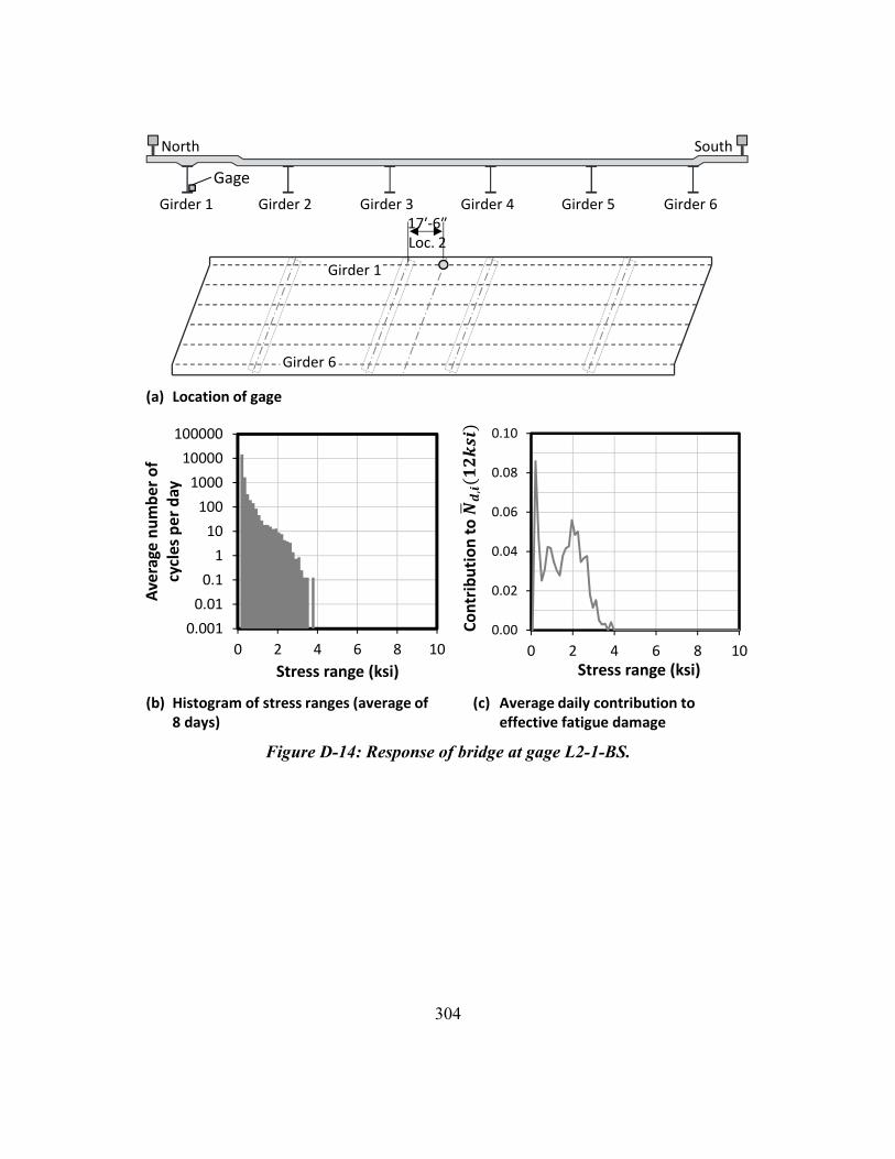
304


0.00

0.02

0.04

0.06

0.08

0.10



Girder 6

Girder 1

Girder 1

North


South

0.001

0.01

0.1

1

10

100

1000

10000

100000

0 2 4 6 8 10

Ave

rage

nu

mb

er o

f cy

cles

pe

r d

ay

Stress range (ksi)

Gage



17′-6″Loc. 2

Co

ntr

ibu

tio

n t

o

305


0.00

0.01

0.02

0.03



Girder 6

Girder 1

Girder 1

North


South

0.001

0.01

0.1

1

10

100

1000

10000

100000

0 2 4 6 8 10

Ave

rage

nu

mb

er o

f cy

cles

pe

r d

ay

Stress range (ksi)

Gage



17′-6″Loc. 2

Co

ntr

ibu

tio

n t

o

306


0.00

0.01

0.02

0.03



Girder 6

Girder 1

Girder 1

North


South

0.001

0.01

0.1

1

10

100

1000

10000

100000

0 2 4 6 8 10

Ave

rage

nu

mb

er o

f cy

cles

pe

r d

ay

Stress range (ksi)

Gage



17′-6″Loc. 2

Co

ntr

ibu

tio

n t

o

307


0.00

0.04

0.08

0.12

0.16





Girder 6

Girder 1

Girder 1

North


South

0.001

0.01

0.1

1

10

100

1000

10000

100000

0 2 4 6 8 10

Ave

rage

nu

mb

er o

f cy

cles

pe

r d

ay

Stress range (ksi)

Gage

17′-6″Loc. 2

Co

ntr

ibu

tio

n t

o

308


0.00

0.04

0.08

0.12

0.16



Girder 6

Girder 1

Girder 1

North


South

0.001

0.01

0.1

1

10

100

1000

10000

100000

0 2 4 6 8 10

Ave

rage

nu

mb

er o

f cy

cles

pe

r d

ay

Stress range (ksi)

Gage



17′-6″Loc. 2

Co

ntr

ibu

tio

n t

o

309


0.00

0.04

0.08

0.12

0.16

0.20





Girder 6

Girder 1

Girder 1

North


South

0.001

0.01

0.1

1

10

100

1000

10000

100000

0 2 4 6 8 10

Ave

rage

nu

mb

er o

f cy

cles

pe

r d

ay

Stress range (ksi)

Gage

17′-6″Loc. 2

Co

ntr

ibu

tio

n t

o

310


0.00

0.04

0.08

0.12

0.16

0.20



Girder 6

Girder 1

Girder 1

North


South

0.001

0.01

0.1

1

10

100

1000

10000

100000

0 2 4 6 8 10

Ave

rage

nu

mb

er o

f cy

cles

pe

r d

ay

Stress range (ksi)

Gage



17′-6″Loc. 2

Co

ntr

ibu

tio

n t

o

311


0.00

0.01

0.02

0.03

0.04

0.05

0.06

0.07



Girder 6

Girder 1

Girder 1

North


South

0.001

0.01

0.1

1

10

100

1000

10000

100000

0 2 4 6 8 10

Ave

rage

nu

mb

er o

f cy

cles

pe

r d

ay

Stress range (ksi)

Gage



20′-0″Loc. 3

Co

ntr

ibu

tio

n t

o

312


0.00

0.01

0.02

0.03



Girder 6

Girder 1

Girder 1

North


South

0.001

0.01

0.1

1

10

100

1000

10000

100000

0 2 4 6 8 10

Ave

rage

nu

mb

er o

f cy

cles

pe

r d

ay

Stress range (ksi)

Gage



20′-0″Loc. 3

Co

ntr

ibu

tio

n t

o

313


0.00

0.02

0.04

0.06

0.08

0.10





Girder 6

Girder 1

Girder 1

North


South

0.001

0.01

0.1

1

10

100

1000

10000

100000

0 2 4 6 8 10

Ave

rage

nu

mb

er o

f cy

cles

pe

r d

ay

Stress range (ksi)

Gage

20′-0″Loc. 3

Co

ntr

ibu

tio

n t

o

314


0.00

0.02

0.04

0.06

0.08

0.10



Girder 6

Girder 1

Girder 1

North


South

0.001

0.01

0.1

1

10

100

1000

10000

100000

0 2 4 6 8 10

Ave

rage

nu

mb

er o

f cy

cles

pe

r d

ay

Stress range (ksi)

Gage



20′-0″Loc. 3

Co

ntr

ibu

tio

n t

o

315


0.00

0.01

0.02

0.03



Girder 6

Girder 1

Girder 1

North


South

0.001

0.01

0.1

1

10

100

1000

10000

100000

0 2 4 6 8 10

Ave

rage

nu

mb

er o

f cy

cles

pe

r d

ay

Stress range (ksi)

Gage



20′-0″Loc. 3

Co

ntr

ibu

tio

n t

o

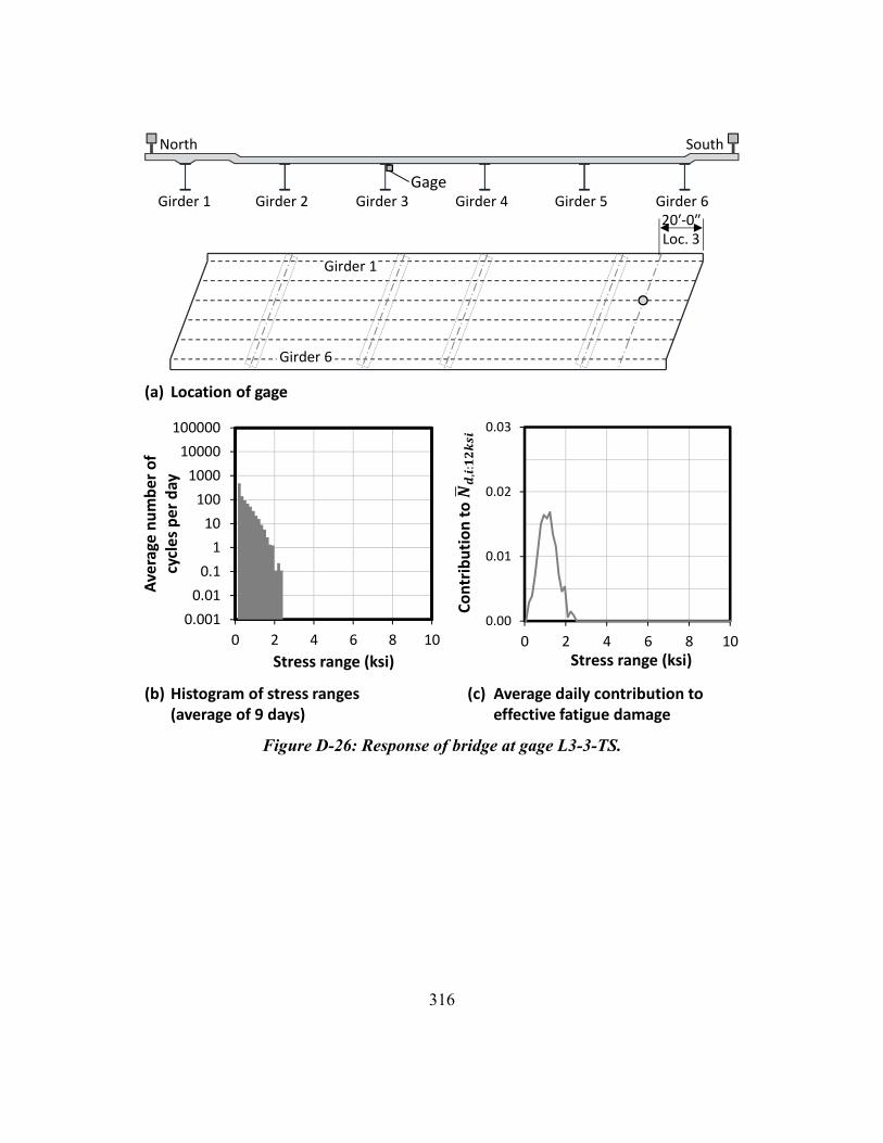
316


0.00

0.01

0.02

0.03



Co

ntr

ibu

tio

n t

o

Girder 6

Girder 1

Girder 1

North


South

0.001

0.01

0.1

1

10

100

1000

10000

100000

0 2 4 6 8 10

Ave

rage

nu

mb

er o

f cy

cle

s p

er

day

Stress range (ksi)

Gage



20′-0″Loc. 3

317


0.00

0.04

0.08

0.12

0.16

0.20

0.24





Girder 6

Girder 1

Girder 1

North


South

0.001

0.01

0.1

1

10

100

1000

10000

100000

0 2 4 6 8 10

Ave

rage

nu

mb

er o

f cy

cles

pe

r d

ay

Stress range (ksi)

Gage

20′-0″Loc. 3

Co

ntr

ibu

tio

n t

o

318


0.00

0.04

0.08

0.12

0.16

0.20

0.24



Girder 6

Girder 1

Girder 1

North


South

0.001

0.01

0.1

1

10

100

1000

10000

100000

0 2 4 6 8 10

Ave

rage

nu

mb

er o

f cy

cles

pe

r d

ay

Stress range (ksi)

Gage



20′-0″Loc. 3

Co

ntr

ibu

tio

n t

o

319


0.00

0.02

0.04

0.06

0.08

0.10

0.12





Girder 6

Girder 1

Girder 1

North


South

0.001

0.01

0.1

1

10

100

1000

10000

100000

0 2 4 6 8 10

Ave

rage

nu

mb

er o

f cy

cles

pe

r d

ay

Stress range (ksi)

Gage

20′-0″Loc. 3

Co

ntr

ibu

tio

n t

o

320


0.00

0.02

0.04

0.06

0.08

0.10

0.12



Girder 6

Girder 1

Girder 1

North


South

0.001

0.01

0.1

1

10

100

1000

10000

100000

0 2 4 6 8 10

Ave

rage

nu

mb

er o

f cy

cles

pe

r d

ay

Stress range (ksi)

Gage



20′-0″Loc. 3

Co

ntr

ibu

tio

n t

o

321


0.00

0.04

0.08

0.12

0.16

0.20

0.24





Girder 6

Girder 1

Girder 1

North


South

0.001

0.01

0.1

1

10

100

1000

10000

100000

0 2 4 6 8 10

Ave

rage

nu

mb

er o

f cy

cles

pe

r d

ay

Stress range (ksi)

Gage

20′-0″Loc. 3

Co

ntr

ibu

tio

n t

o

322


0.00

0.04

0.08

0.12

0.16

0.20

0.24



Girder 6

Girder 1

Girder 1

North


South

0.001

0.01

0.1

1

10

100

1000

10000

100000

0 2 4 6 8 10

Ave

rage

nu

mb

er o

f cy

cles

pe

r d

ay

Stress range (ksi)

Gage



20′-0″Loc. 3

Co

ntr

ibu

tio

n t

o

323

APPENDIX E

Strain data from Bridge D

The average stress spectrum and contribution to fatigue damage ( , 12 ) for

all strain gages at Bridge D are presented in this Appendix. The average daily fatigue

damage at Bridge D is summarized in Table E-1 for all of the gages installed on the

bottom flange.

Table E-1: Summary of daily fatigue damage at Bridge D.

Loc

atio

n

Gir

der

Fla

nge


days monitored

,

L1 2 BN 7.18 0.60 150,000 4 18.8

L1 3 BS 4.86 0.63 125,000 4 17.7

L2 3 BS 2.68 0.36 95,000 4 2.52

L3 2 BN 5.73 0.59 133,000 4 15.6

L3 3 BS 4.71 0.58 129,000 4 14.4

324

Figure E-1: Response of bridge at gage L1-2-TN.

0.00

0.02

0.04

0.06

0.08

0.10


0.001

0.01

0.1

1

10

100

1000

10000

100000

0 2 4 6 8 10

Ave

rage

nu

mb

er o

f cy

cles

per

day

Stress range (ksi)


Gage



South

Girder 1

North

Girder 2 Girder 3 Girder 4 Girder 5 Girder 6 Girder 765′-0″ Loc. 1

Girder 1

Girder 7

Co

ntr

ibu

tio

n t

o

325

Figure E-2: Response of bridge at gage L1-2-BN.

0.0

0.4

0.8

1.2

1.6

2.0


Girder 2

0.001

0.01

0.1

1

10

100

1000

10000

100000

0 2 4 6 8 10

Ave

rage

nu

mb

er o

f cy

cles

per

day

Stress range (ksi)


Gage



South

Girder 1

North

Girder 3 Girder 4 Girder 5 Girder 6 Girder 765′-0″ Loc. 1

Girder 1

Girder 7

Co

ntr

ibu

tio

n t

o

326

Figure E-3: Response of bridge at gage L1-3-TS.

0.00

0.02

0.04

0.06

0.08

0.10

0.12


0.001

0.01

0.1

1

10

100

1000

10000

100000

0 2 4 6 8 10

Ave

rage

nu

mb

er o

f cy

cles

per

day

Stress range (ksi)


Gage



South

Girder 1

North

Girder 2 Girder 3 Girder 4 Girder 5 Girder 6 Girder 765′-0″ Loc. 1

Girder 1

Girder 7

Co

ntr

ibu

tio

n t

o

327

Figure E-4: Response of bridge at gage L1-3-BS.

0.0

0.4

0.8

1.2

1.6

2.0

2.4

2.8


Girder 2

0.001

0.01

0.1

1

10

100

1000

10000

100000

0 2 4 6 8 10

Ave

rage

nu

mb

er o

f cy

cles

per

day

Stress range (ksi)


Gage



South

Girder 1

North

Girder 3 Girder 4 Girder 5 Girder 6 Girder 765′-0″ Loc. 1

Girder 1

Girder 7

Co

ntr

ibu

tio

n t

o

328


0.00

0.02

0.04

0.06

0.08

0.10


0.001

0.01

0.1

1

10

100

1000

10000

100000

0 2 4 6 8 10

Ave

rage

nu

mb

er o

f cy

cles

per

day

Stress range (ksi)


Gage



South

Girder 1

North


Girder 1

Girder 7

20′-0″ Loc. 2

Co

ntr

ibu

tio

n t

o

329


0.0

0.2

0.4

0.6

0.8

1.0


Girder 2

0.001

0.01

0.1

1

10

100

1000

10000

100000

0 2 4 6 8 10

Ave

rage

nu

mb

er o

f cy

cles

per

day

Stress range (ksi)


Gage



South

Girder 1

North


Girder 1

Girder 7

20′-0″ Loc. 2

Co

ntr

ibu

tio

n t

o

330

Figure E-7: Response of bridge at gage L3-2-BN.

0.0

0.4

0.8

1.2

1.6

2.0


Girder 2

0.001

0.01

0.1

1

10

100

1000

10000

100000

0 2 4 6 8 10

Ave

rage

nu

mb

er o

f cy

cles

per

day

Stress range (ksi)


Gage



South

Girder 1

North


Girder 1

Girder 7

54′-0″ Loc. 3

Co

ntr

ibu

tio

n t

o

331


0.00

0.04

0.08

0.12

0.16

0.20


0.001

0.01

0.1

1

10

100

1000

10000

100000

0 2 4 6 8 10

Ave

rage

nu

mb

er o

f cy

cles

per

day

Stress range (ksi)


Gage



South

Girder 1

North


Girder 1

Girder 7

54′-0″ Loc. 3

Co

ntr

ibu

tio

n t

o

332


0.0

0.4

0.8

1.2

1.6

2.0

2.4

2.8


Girder 2

0.001

0.01

0.1

1

10

100

1000

10000

100000

0 2 4 6 8 10

Ave

rage

nu

mb

er o

f cy

cles

per

day

Stress range (ksi)


Gage



South

Girder 1

North


Girder 1

Girder 7

54′-0″ Loc. 3

Co

ntr

ibu

tio

n t

o

333

References

AASHTO. (1990). Guide Specifications for Fatigue Evaluation of Existing Steel Bridges.

Washington, D.C.: American Association of State Highway and Transportation

Officials.

AASHTO. (2010). LRFD Bridge Design Specifications. Washington, D.C.: American

Association of State Highway and Transportation Officials.

AASHTO. (2011). The Manual for Bridge Evaluation. Washington, D.C.: American

Association of State Highway and Transportation Officials.

Alampalli, S., and Lund, R. (2006). Estimating Fatigue Life of Bridge Components Using

Measured Strains. Journal of Bridge Engineering, 11(6), 725-736.

ASCE. (1982). Fatigue Reliabilty: Variable Amplitude Loading. Journal of the Structural

Division, 108(ST1), 47-69.

ASTM. (2011). E1049-85: Standard Practices for Cycle Counting in Fatigue Analysis.

West Conshohocken: ASTM International.

Barsom, J., and Rolfe, S. (1999). Fracture and Fatigue Control in Structures:

Applications of Fracture Mechanics (3rd ed.). West Conshohocken, PA: ASTM.

Bocchini, P., and Frangopol, D. (2011). A Probabilistic Computational Framework for

Bridge Network Optimal Maintenance Scheduling. Reliability Engineering and

System Safety, 96, 332-349.

Bowman, M., Fu, G., Zhou, Y., Connor, R., and Godbole, A. (2012). Fatigue Evalution

of Steel Bridges. Washington, DC: Transportation Research Board.

Chotickai, P., and Bowman, M. (2006). Comparative Study of Fatigue Provisions for the

AASHTO Fatigue Guide Specifications and LRFR Manual for Evaluation.

Journal of Bridge Engineering, 11(5), 655-660.

Chung, H. (2004). Fatigue Reliability and Optimal Inspection Strategies for Steel

Bridges. Austin, TX: The University of Texas at Austin. Dissertation.

334

Connor, R., and Fisher, J. (2006). Identifying Effective and Ineffective Retrofits for

Distortion Fatigue Cracking in Steel Bridges Using Field Instrumentation. Journal

of Bridge Engineering, 11(6), 745-752.

Dierks, E. (2011). Design of an Electromagnetic Vibration Energy Harvester for

Structural Health Monitoring of Bridges Employing Wireless Sensor Networks.

Austin, TX: The University of Texas at Austin. Thesis.

Dowling, N. (1972). Fatigue Failure Predictions for Complicated Stress-Strain Histories.

Journal of Materials, 7(1), 71-87.

Downing, S., and Socie, D. (1982). Simple Rainflow Counting Algorithms. International

Journal of Fatigue, 4(1), 31-40.

ECCS Technical Committee 6. (1985). Recommendations for the Fatigue Design of Steel

Structures. Rotterdam: European Convention for Constructional Steelwork.

Fasl, J., Helwig, T., Wood, S., Samaras, V., Yosef, A., Frank, K., Potter, D, and

Lindenberg, R. (2010). Development of Rapid, Reliable, and Economical

Methods for Inspection and Monitoring of Highway Bridges. IABMAS 2010.

Philadelphia: Taylor & Francis.

Fasl, J., Samaras, V., Reichenbach, M., Helwig, T., Wood, S., Potter, D., Lindenberg, R.,

and Frank, K. (2012a). Develoment of a Wireless Strain Node and the Software to

Monitor Fracture-Critical Bridges. Sensors and Smart Structures Technologies for

Civil, Mechanical, and Aerospace Systems. San Diego: International Society for

Optical Engineering.

Fasl, J., Helwig, T., Wood, S., Pasupathy, P., Neikirk, D., and Raffaeli, F. (2012b).

Factors Affecting Wireless Network Communication in Monitoring Systems for

Steel Bridges. Journal of Civil Structural Health Monitoring, 2(2), 87-95.

doi:10.1007/s13349-012-0019-y

Fasl, J., Samaras, V., Reichenbach, M., Helwig, T., Wood, S., Potter, D., Lindenberg, R.,

and Frank, K. (2012c). Evaluating Fatigue Damage Using Strain Data.

Conference Proceedings of NDE/NDT for Highways and Bridges: Structural

335

Materials Technology. New York, NY: American Society for Nondestructive

Testing.

Federal Highway Administration. (2012). MAP-21 - Moving Ahead for Progress in the

21st Century. Retrieved August 28, 2012, from http://www.fhwa.dot.gov/map21/

Fish, J. (1977). Bridge Fatigue Guide: Design and Details. Chicago, IL: American

Institute of Steel Construction.

Fisher, J., Frank, K., Hurt, M., and McNamee, B. (1970). Effect of Weldments on the

Fatigue Strength of Steel Beams. Washington, D.C.: Transportation Research

Board.

Fisher, J., Albrecht, P., Yen, B., Klingerman, D., and McNamee, B. (1974). Fatigue

Strength of Steel Beams with Welded Stiffeners and Attachments. Washington,

D.C.: Transportation Research Board.

Fisher, J., Mertz, D., and Zhong, A. (1983). Steel Bridge Members Under Variable

Amplitude Long Life Fatigue Loading. Washington, D.C.: Transportation

Research Board.

Fisher, J., Kulak, G., and Smith, I. (1998). A Fatigue Primer for Structural Engineers.

Chicago, IL: National Steel Bridge Alliance.

Fisher, J., Nussbaumer, A., Keating, P., and Yen, B. (1993). Resistance of Welded Details

Under Variable Amplitude Long-Life Fatigue Loading. Washington, D.C.:

Transportation Research Board.

Inamdar, S. (2012). Design of a Solar Energy Harvesting System for Structural Health

Monitoring Systems. Austin, TX: The University of Texas at Austin. Thesis.

Keating, P., and Fisher, J. (1986). Evaluation of Fatigue Tests and Design Criteria on

Welded Details. Washington, DC: Transportation Research Board.

Keating, P., Halley, S., and Fisher, J. (1986). Fatigue Test Database for Welded Steel

Bridge Details. Bethlehem, PA: Lehigh University. Report 488.2.

Kim, S.-H., Lee, S.-W., and Mha, H.-S. (2001). Fatigue Reliability Assessment of an

Existing Steel Railroad Bridge. Engineering Structures, 23, 1203-1211.

336

Kwon, K., and Frangopol, D. (2010). Bridge Fatigue Reliability Assessment Using

Probability Density Functions of Equivalent Stress Range Based on Field

Monitoring Data. International Journal of Fatigue, 32, 1221-1232.

Leander, J., Andersson, A., and Karoumi, R. (2010). Monitoring and Enhanced Fatigue

Evaluation of a Steel Railway Bridge. Engineering Structures, 32, 854-863.

Li, Z., Chan, T., and Ko, J. (2001). Fatigue Analysis and Life Prediction of Bridges with

Structural Health Monitoring Data - Part I: Methodology and Strategy.

International Journal of Fatigue, 23, 45-53.

Liu, M., Frangopol, D., and Kwon, K. (2010). Fatigue Reliability Assessment of

Retrofitted Steel Bridges Integrating Monitored Data. Structural Safety, 32, 77-

89.

Lynch, J., Sundararajan, A., Law, K., Kiremidjian, A., and Carryer, E. (2004).

Embedding Damage Detection Algorithms in a Wireless Sensing Unit for

Operation Power Efficiency. Smart Materials and Structures, 13(4), 800-810.

McEvoy, T. (2011). Wind Energy Harvesting for Bridge Health Monitoring. Austin, TX:

The University of Texas at Austin. Thesis.

Miner, M. (1945). Cumulative Damage in Fatigue. Journal of Applied Mechanics, 12,

A159-A164.

Moore, M., Phares, B., Graybeal, B., Rolander, D., and Washer, G. (2000). Reliability of

Visual Inspection for Highway Bridges. FHWA NDE Validation Center.

Moses, F., Schilling, C., and Raju, K. (1987). Fatigue Evaluation Procedures for Steel

Bridges. Washington, D.C.: Transportation Research Board.

Munse, W. (1964). Fatigue of Welded Steel Structures. New York, NY: Welding

Research Council.

National Bridge Inventory. (2008). Age Distribution of Highway Bridges in the US.

Retrieved July 28, 2012, from http://www.nationalbridges.com.

National Instruments. (2012). NI WSN-3214 User Guide and Specifications. Retrieved

November 26, 2012, from htto://www.ni.com.

337

Orcesi, A., Frangopol, D., and Kim, S. (2010). Optimization of Bridge Maintenance

Strategies Based on Multiple Limit States and Monitoring. Engineering

Structures, 32, 627-640.

Paris, P., Gomez, M., and Anderson, W. (1961). A Rational Analytic Theory of Fatigue.

The Trend in Engineering, 13, 9-14.

Reichenbach, M. (2012). Evaluating Vehicular-Induced Vibrations of Typical Highway

Bridges for Energy Harvesting Applications. Austin, TX: The University of Texas

at Austin. Thesis

Samaras, V., Fasl, J., Reichenbach, M., Helwig, T., Wood, S., and Frank, K. (2012).

Long-Term Gage Reliability for Structural Health Monitoring of Steel Bridges.

Sensors and Smart Structures Technologies for Civil, Mechanical, and Aerospace

Systems. San Diego: International Society for Optical Engineering.

Samaras, V. (2013). Title TBD. The University of Texas at Austin. Dissertation.

Schilling, C., Klippstein, K., Barsom, J., and Blake, G. (1978). Fatigue of Welded Steel

Bridge Members Under Variable-Amplitude Loadings. Washington, D.C.:

Transportation Research Board.

Swenson, K., and Frank, K. (1984). The Application of Cumulative Damage Fatigue

Theory to Highway Bridge Fatigue Design. Austin, TX: Center for Transportation

Research.

Szerszen, M., Nowak, A., and Laman, J. (1999). Fatigue Reliability of Steel Bridges.

Journal of Constructional Steel Research, 52, 83-92.

Tanaka, S., and Akita, S. (1975). On the Miner's Damage Hypothesis in Notched

Specimens with Emphasis on Scatter of Fatigue Life. Engineering Fracture

Mechanics, 7, 473-480.

USDOT. (2006). 2004 Status of the Nation's Highways, Bridges, and Transit: Conditions

& Performance. Retrieved from http://www.fhwa.dot.gov/policy/2004cpr/

Weaver, J. (2011). Innovative Energy Harvesting Technology for Wireless Bridge

Monitoring Systems. Austin, TX: The University of Texas at Austin. Dissertation.

338

Wirsching, P. (1984). Fatigue Reliability for Offshore Structures. Journal of Structural

Engineering, 110(10), 2340-2356.

Wirsching, P., and Chen, Y. (1988). Consideration of Probability-Based Fatigue Design

for Marine Structures. Marine Structures, (1), 23-45.

Zhao, Z., Haldar, A., and Breen, F. (1994). Fatigue-Reliability Updating through

Inspections of Steel Bridges. Journal of Structural Engineering, 120(5), 1624-

1641.

Zhou, Y. (2006). Assessment of Bridge Remaining Fatigue Life Through Field Strain

Measurement. Journal of Bridge Engineering, 11(6), 737-744.

Zimowski, K. (2012). Next Generation Wind Energy Harvester to Power Bridge Health

Monitoring Systems. Austin, TX: The University of Texas at Austin. Thesis.

copyright by jeremiah david fasl 2013

Documents