Copyright

by

David James Love

2004

The Dissertation Committee for David James Love

certifies that this is the approved version of the following dissertation:

Feedback Methods for Multiple-Input

Multiple-Output Wireless Systems

Committee:

Robert W. Heath, Jr., Supervisor

Gustavo de Veciana

John E. Gilbert

Edward J. Powers

Theodore S. Rappaport

Sanjay Shakkottai

Feedback Methods for Multiple-Input

Multiple-Output Wireless Systems

by

David James Love, B.S., M.S.E.

Dissertation

Presented to the Faculty of the Graduate School of

The University of Texas at Austin

in Partial Fulfillment

of the Requirements

for the Degree of

Doctor of Philosophy

The University of Texas at Austin

May 2004

Dedicated to the memory of my grandfathers,

Joe B. Stuart and Ralph D. Love

Acknowledgments

I would like to start by thanking God for the many blessings in my life. I thank

my parents Jim and Priscilla Love for their support throughout my education.

All of my academic successes can be traced back to them. In elementary school

my parents told me, “All we expect is for you to do your best.” I am happy

to say that I took this lesson to heart. My wife Elaina Love has also been

instrumental to my academic life. Many people do not realize that we have

been together since I was fifteen. I love her very much, and I (along with most

of my important documents) would be lost without her. My younger brother

Brian Love has also played a large role in my success. I always tried to present

myself as a role model for Brian and doing so has made me a better person. My

life has also been profoundly affected by my grandparents Joe and Ola Stuart

and Ralph and Jane Love. Just like my parents, they always encouraged me

to do my best. Though my grandfathers have both passed away, I hope that

my success makes them proud.

I would like to thank my advisor Robert Heath for serving as a friend

and mentor during my graduate studies. Robert gave me a large amount of

freedom during graduate school, and I feel that this freedom was fundamental

to my accomplishments. I am grateful to my committee members Gustavo de

v

Veciana, John Gilbert, Edward Powers, Ted Rappaport, and Sanjay Shakkot-

tai. Their comments and insights made my research more fruitful. I would like

to thank Alan Bovik for his generosity in allowing me to work with his research

group early in my graduate studies. John Dollard and Lawrence Shepley have

provided invaluable advice and help throughout my UT years. I would also

like to thank Brian Evans and Irwin Sandberg for their support.

Thanks also goes to everyone who I interacted with at the Texas In-

struments DSPS R&D Center in Dallas. Without the help of Mike Polley and

Don Shaver, I would have never had the opportunity to be associated with TI.

Anuj Batra, Hank Eilts, Srinath Hosur, and David Magee have all provided

useful guidance.

I would also like to thank my friends. Joseph D’Auria has provided

enough entertainment to supplant television. Joe and I have experienced ad-

ventures rivaling those on Seinfeld. My UT ECE days have been filled with

wonderful memories thanks to my LIVE friends such as Umesh Rajashekar,

Farooq Sabir, Hamid Sheikh, and Mehul Sampat. We have spent many hours

discussing problems in signal processing, communications, ping-pong, and ar-

ranged marriages. My WSIL friends including Manish Airy, Runhua Chen,

Antonio Forenza, Chun-Hung Liu, Caleb Lo, Bishwarup Mondal, Roopsha

Samanta, Taiwen Tang, and Jimmy Wang have provided loads of laughs and

Silicon Valley stories.

I would also like to thank The University of Texas at Austin. I have been

at UT for my entire university life. I have been lucky enough to watch Ricky

Williams, Major Applewhite, and T.J. Ford in person. Joe, Brian, and I were

even fortunate enough to get a “Thanks guys!” from Mack Brown during the

Cotton Bowl practices at SMU during the 1999 season. I got to see the highs

vi

(Heisman, UT Final Four, Holiday Bowl comeback) and lows (UCLA, Big 12

title game meltdown, various OU shellackings). UT football and basketball

have been my primary pastime and passion. I will always bleed burnt orange.

David James Love

The University of Texas at Austin

May 2004

vii

Feedback Methods for Multiple-Input

Multiple-Output Wireless Systems

Publication No.

David James Love, Ph.D.

The University of Texas at Austin, 2004

Supervisor: Robert W. Heath, Jr.

The availability and performance of wireless communication systems have

grown at unprecedented rates over the last fifteen years. In order to maintain

these growth rates, next generation wireless systems must supply both reliabil-

ity and high data rates using a fixed amount of spectrum and limited transmit

power. Multiple-input multiple-output (MIMO) wireless communication sys-

tems, which use multiple antennas at both the transmitter and receiver, are

expected to be one of the enabling technologies for next generation wireless

systems. MIMO wireless systems provide both data rate and reliability im-

provements by designing signals over space as well as time and/or frequency.

One of the key features of wireless links is the phenomenon known as

fading. In a narrowband wireless link, fading can be modeled as a multiplica-

tive channel gain. Many of the benefits promised by MIMO wireless systems

will not be realized without the availability of channel gain information at the

viii

transmitter. Current research focuses on the usage of MIMO signaling where

the transmitter does not have any kind of channel information. When some

form of channel information is available, however, the MIMO signal can be

adapted to the current channel conditions to improve performance. Unfor-

tunately, many wireless systems will not have any form of a priori channel

knowledge without feedback from the receiver to transmitter. Because feed-

back will occupy a percentage of the data-rate in the reverse wireless link

(i.e. the wireless link where the receiver terminal serves as the transmitter),

feedback must be kept to a limited number of bits.

This dissertation describes new, practical methods for limited feedback

space-time signaling. It develops space-time techniques that provide improved

performance when channel information, in the form of a fixed number of bits,

is conveyed from the receiver to the transmitter. Limited feedback techniques

are developed for linearly precoded orthogonal space-time block codes and lin-

early precoded spatial multiplexing. A new adaptive modulation technique

for linearly precoded spatial multiplexing called multi-mode precoding is pre-

sented. Past research in the area of space-time signaling is also overviewed.

ix

Contents

Acknowledgments v

Abstract viii

Chapter 1 Introduction 1

1.1 Wireless Communications . . . . . . . . . . . . . . . . . . . . 1

1.2 Multiple-Input Multiple-Output Wireless Systems . . . . . . . 3

1.3 Closed-Loop Space-Time Signaling . . . . . . . . . . . . . . . 4

1.4 Contributions . . . . . . . . . . . . . . . . . . . . . . . . . . . 7

1.5 Organization of Dissertation . . . . . . . . . . . . . . . . . . . 9

Chapter 2 Background 10

2.1 Notation . . . . . . . . . . . . . . . . . . . . . . . . . . . . . . 10

2.2 System Model . . . . . . . . . . . . . . . . . . . . . . . . . . . 11

2.3 Beamforming . . . . . . . . . . . . . . . . . . . . . . . . . . . 13

2.4 Spatial Multiplexing . . . . . . . . . . . . . . . . . . . . . . . 14

2.4.1 Open-Loop . . . . . . . . . . . . . . . . . . . . . . . . 14

2.4.2 Closed-Loop Precoding . . . . . . . . . . . . . . . . . . 15

2.5 Orthogonal Space-Time Block Coding . . . . . . . . . . . . . . 18

x

2.5.1 Open-Loop . . . . . . . . . . . . . . . . . . . . . . . . 19

2.5.2 Closed-Loop Precoding . . . . . . . . . . . . . . . . . . 20

2.6 Diversity-Multiplexing Tradeoff . . . . . . . . . . . . . . . . . 21

Chapter 3 Limited Feedback Precoding for Space-Time Codes 23

3.1 System Overview . . . . . . . . . . . . . . . . . . . . . . . . . 23

3.2 Selection Criterion . . . . . . . . . . . . . . . . . . . . . . . . 26

3.3 Chordal Distance Precoding: Motivation and Codebook Design 29

3.3.1 Distortion Function . . . . . . . . . . . . . . . . . . . . 29

3.3.2 Codebook Design Criterion . . . . . . . . . . . . . . . 32

3.3.3 Practical Codebook Designs . . . . . . . . . . . . . . . 34

3.4 Performance Analysis . . . . . . . . . . . . . . . . . . . . . . . 36

3.5 Simulations . . . . . . . . . . . . . . . . . . . . . . . . . . . . 39

Chapter 4 Limited Feedback Precoding for Spatial Multiplexing 46

4.1 System Overview . . . . . . . . . . . . . . . . . . . . . . . . . 47

4.2 Precoding Criteria . . . . . . . . . . . . . . . . . . . . . . . . 49

4.2.1 Maximum Likelihood Receiver . . . . . . . . . . . . . . 50

4.2.2 Linear Receiver . . . . . . . . . . . . . . . . . . . . . . 51

4.2.3 Capacity . . . . . . . . . . . . . . . . . . . . . . . . . . 54

4.3 Limited Feedback Precoding: Motivation and Codebook Design 56

4.3.1 Probabilistic Characterization of Optimal Precoding Ma-

trix . . . . . . . . . . . . . . . . . . . . . . . . . . . . . 56

4.3.2 Grassmannian Subspace Packing . . . . . . . . . . . . 57

4.3.3 Codebook Design Criteria . . . . . . . . . . . . . . . . 61

4.4 Simulations . . . . . . . . . . . . . . . . . . . . . . . . . . . . 66

xi

Chapter 5 Multi-Mode Precoding 73

5.1 System Overview . . . . . . . . . . . . . . . . . . . . . . . . . 74

5.2 Multi-Mode Precoder Selection . . . . . . . . . . . . . . . . . 76

5.2.1 Performance Discussion . . . . . . . . . . . . . . . . . 77

5.2.2 Selection Criteria . . . . . . . . . . . . . . . . . . . . . 80

5.2.3 Minimum Distance Calculations . . . . . . . . . . . . . 83

5.3 Multi-Mode Precoding: Perfect Transmitter Channel Knowledge 84

5.4 Limited Feedback Multi-Mode Precoding: Zero Transmitter Chan-

nel Knowledge . . . . . . . . . . . . . . . . . . . . . . . . . . . 86

5.4.1 Codebook Model . . . . . . . . . . . . . . . . . . . . . 86

5.4.2 Codeword Distribution . . . . . . . . . . . . . . . . . . 87

5.4.3 Codebook Criterion Given the Number of Substreams . 91

5.5 Diversity Order & Multiplexing Gain . . . . . . . . . . . . . . 92

5.6 Relation to Covariance Quantization . . . . . . . . . . . . . . 93

5.7 Simulations . . . . . . . . . . . . . . . . . . . . . . . . . . . . 94

Chapter 6 Practical Aspects 102

6.1 Effect of Spatial Correlation . . . . . . . . . . . . . . . . . . . 102

6.2 Effect of Feedback Delay . . . . . . . . . . . . . . . . . . . . . 117

6.3 Effect of Channel Estimation Error . . . . . . . . . . . . . . . 120

6.4 Feedback Error . . . . . . . . . . . . . . . . . . . . . . . . . . 123

6.5 Application to Broadband Communications . . . . . . . . . . 125

Chapter 7 Conclusions 127

7.1 Summary . . . . . . . . . . . . . . . . . . . . . . . . . . . . . 127

7.2 Future Work . . . . . . . . . . . . . . . . . . . . . . . . . . . . 128

xii

Bibliography 130

Vita 147

xiii

Chapter 1

Introduction

This chapter presents an introduction and overview of this dissertation. Sec-

tion 1.1 gives a general introduction to wireless. In Section 1.2, the basic ideas

behind multiple-input multiple-output (MIMO) wireless systems are reviewed.

Current and past research into closed-loop MIMO wireless is presented in Sec-

tion 1.3. The contributions are briefly summarized in Section 1.4. A summary

of the organization of the remaining chapters is presented in Section 1.5.

1.1 Wireless Communications

Wireless communications have forever changed the way we live because of their

ability to supply ubiquitous voice and data communications. Internet appli-

cations and appliances have fueled research in wireless systems that supply

data rates much larger than those found in wireless voice communications.

With second and a half generation (2.5G) and third generation (3G) commu-

nications becoming commercially viable, it is clear that the future of wireless

communications is in wireless appliances that can provide both voice and data

1

communications over a reliable and high rate link.

In designing a wireless system, designers must deal with the scarcity

of the available bandwidth. Purchasing a licensed band requires a several

hundred billion dollar investment. Unlicensed bands, in contrast, are free to

use but are unregulated. Both licensed and unlicensed bands are limited in

the amount of bandwidth allotted. Thus system designers can not look to an

increase in bandwidth in designing next generation wireless communication

systems.

Operating over a fixed bandwidth means that a high spectral efficiency

is required. Spectral efficiency is defined as the bits per second transmitted

divided by the system bandwidth (in Hertz). The capacity of a wireless link is

the largest spectral efficiency that can be reliably obtained for a given amount

of bandwidth. Thus, we would like to choose a wireless link with a large

capacity so that we can obtain a good spectral efficiency when operating.

Wireless systems must also operate reliably. They must maintain the

same link quality that is found in wireline communications. In communication

theory, reliability quantitatively is described by the probability of error at

the receiver. A reliable link will have a low probability of error. Variations

in the received signal strength due to mobile motion and the propagation

environment make link reliability a challenging problem.

Transmit power is another commodity in wireless system design. Un-

fortunately, transmit power is also limited because of issues such as battery

power, Federal Communications Commission (FCC) regulations, and health

concerns. Transmit power, therefore, can not be used as a solution to the

spectral efficiency and reliability design challenges. System designers must in-

stead look to smart communications and signal processing algorithms for next

2

generation communications.

1.2 Multiple-Input Multiple-Output Wireless

Systems

One solution to the problem of simultaneously maximizing spectral efficiency

and reliability is the use of wireless systems employing multiple antennas at

both the transmitter and receiver, also known as multiple-input multiple-

output (MIMO) wireless systems. MIMO wireless systems provide gains in

Shannon capacity and link reliability over single-antenna wireless systems by

signaling over the spatial dimension of a wireless link [1]–[3].

The concept behind the MIMO capacity gain can be understood from

the use of sufficiently spaced multiple antennas. Multiple antenna receivers

have been used for over fifty years in receive combining systems (see for ex-

ample [4], [5]). Multiple antenna transmitters were studied in [6] for use with

single antenna receivers. Paulraj and Kailath proposed using a multiple an-

tenna transmitter and receiver [7], however, it was not until Telatar’s work

in [1], [8] that the effect of a multiple antenna transmitter and receiver on the

capacity was fully understood.

Multiple antenna technology has been standardized in wireless metropoli-

tan access networks [9], wideband code division multiple access (WCDMA) [10]

and is expected to be a critical component of next-generation wireless local

area networks (LANs) [11]. Most of the major industrial focus, however, has

been limited to two transmit and/or receive antennas due to practical consid-

erations. Because of the performance gains that larger transmit and receive

3

antenna arrays can provide, it is of utmost importance for researchers to find

practical methods to take advantage of the MIMO capacity.

1.3 Closed-Loop Space-Time Signaling

The concept of space-time coding was introduced in [12]–[14]. Space-time

codes work using sophisticated signal processing at both the transmitter and

receiver to leverage the MIMO spatial diversity advantage. Space-time coding

has become synonymous with open-loop∗ MIMO transmission. Space-time

codes improve performance over single-antenna modulation schemes but lose

array gain compared with other space-time techniques because they do not

use any kind of channel information [15], [16].

An alternative signaling method to space-time coding is spatial multi-

plexing [3],[16],[17]. In spatial multiplexing systems, a single symbol stream is

demultiplexed into multiple symbol streams. Each symbol stream is assigned

to a transmit antenna, and the symbols are then transmitted without the ben-

efit of any transmit spatial diversity. Spatial multiplexing is often not thought

of as a space-time code because there is no spatial or temporal redundancy

(i.e. each symbol is only sent over one antenna during one transmission) [16].

Closed-loop† MIMO transmission originated with the extension of beam-

forming and combining to MIMO channels [18]. In beamforming, a transmit-

ted symbol is projected onto a data vector that is then sent from a multiple-

antenna transmitter (i.e. each entry of the vector is sent to a different transmit

∗Open-loop transmission is defined as signaling without any knowledge of the channel.This means that the space-time signals are designed without respect to the current channelconditions, average channel parameters, or receiver feedback.

†Closed-loop transmission is defined as signaling with some form of channel knowledgeor feedback from the receiver.

4

antenna). Combining works by linearly weighting and summing the outputs

of multiple receive antennas to yield an estimate of the transmitted signal.

The idea with this early work was to convert the MIMO matrix channel into a

single-input single-output channel that was resilient to fading. MIMO beam-

forming and combining were later studied in [19]–[27] for the case where exact

channel state information (CSI) was available at the transmitter.

The ideas behind the single substream (i.e. only one symbol transmitted

at each channel use) beamforming and combining methods were extended to

multiple substream (or equivalently spatial multiplexing [3]) linear precoding

systems in [28]–[35]. Linear precoding can be understood as sending a vector

obtained from right-multiplying a symbol vector, a multi-dimensional complex

column vector, by a precoding matrix. These precoding methods were based

on a variety of assumptions about the transmitter’s channel knowledge such as

full CSI [28],[29], knowledge of the first-order statistics [30]–[32], or knowledge

of the second order statistics of the channel [33]–[35].

Precoded spatial multiplexing is actually a combination of beamforming

and spatial multiplexing because the number of substreams is reduced to allow

for spatial redundancy. Systems that make tradeoffs such as this will be defined

as diversity-multiplexing tradeoff systems. Diversity gain and multiplexing

gain are two parameters of a space-time signaling strategy that can be given

explicit mathematical definitions [36]. Beamforming and space-time coding

are two transmission techniques that achieve maximum diversity gain [12],

[14], [37], [38], while spatial multiplexing achieves full multiplexing gain [3]. It

was shown in [39] that the number of substreams transmitted can be adapted

based on current CSI to simultaneously maximize both parameters. A multi-

mode diversity-multiplexing tradeoff was studied in [40] by varying the number

5

of antennas used for transmission. Because of the precoding interpretation of

antenna selection, this can be thought of as an adaptive precoder.

Closed-loop space-time block coding was first introduced in [41] using

complete channel knowledge to decompose the multiple antenna channel into

parallel sub-channels. More practical closed-loop space-time codes were pro-

posed in [32],[42]–[51]. All of these references use some form of linear precoding

by applying a linear transformation to the spatio-temporal block (or matrix)

before transmission.

Most of these closed-loop methods unfortunately require either complete

CSI or statistics of the channel. These assumptions are unrealistic in many

wireless systems such as those using frequency division duplexing since the

forward and reverse channels are approximately independent. For this reason,

more practical methods of closed-loop signaling have been studied where the

receiver sends back a limited number of bits to the transmitter based on current

CSI. These were studied in great detail for beamforming and combining in

[18], [19], [22], [27], [52]–[63].

Introductory work on limited feedback, closed-loop space-time coding

was done in [43]–[48], [51]. Each of these papers restricted the space-time code

to an orthogonal space-time block code (OSTBC) (see [13], [14]) and studied

the problem as an antenna selection problem, where dlog2

(Mt

M

)e bits are allo-

cated for feedback per channel realization for an Mt transmit antenna system

and M antenna space-time code, or as a problem of directly quantizing the

channel. Quantizing the channel, however, should in general be avoided be-

cause of the sensitivity of the eigen-structure to quantization error [64] and

the large amount of feedback necessary for even coarse quantization of a ma-

trix channel. For example, a four-by-four MIMO system with entry-by-entry

6

quantization according to two bits per real part and two bits per imaginary

part would require at least 64 bits of quantization! This is a dramatic amount

of feedback for this extremely coarse quantization.

Limited feedback precoding for spatial multiplexing systems has been

addressed only in the context of antenna selection [65]–[71]. While antenna

selection is easily implemented, it suffers in performance because of the restric-

tions on the form of the precoding matrices [72], [73]. Furthermore, antenna

selection does not allow the allocation of more feedback to further improve

performance.

1.4 Contributions

Previous work on closed-loop techniques for MIMO communications shows

that there is great promise in sending partial CSI‡ to the transmitter. Unfor-

tunately, prior work fails to address the fundamental problem of how to provide

CSI to the transmitter optimally using a limited amount of feedback. For this

reason, this dissertation studies limited feedback in MIMO communications.

The work provides a practical solution for implementing high performance,

closed-loop space-time signaling techniques. The proposed techniques could

find application in wireless LANs (ex. the IEEE 802.11N study group), wireless

fixed-base access (ex. the IEEE 802.16 working group), and mobile wireless

access (ex. the IEEE 802.20 working group). The contributions are as follows:

• A limited feedback precoding methodology for orthogonal space-time block

‡Partial CSI is defined as any form of channel knowledge at the transmitter that is notperfect channel knowledge. This includes statistical knowledge, knowledge of a quantizedchannel, knowledge of a quantized beamforming vector, etc.

7

codes transmitting over narrowband, matrix Rayleigh fading channels.

1. Developing a system model where the precoder is chosen from a

finite set, or codebook, of possible precoding matrices designed off-line

and known to both the transmitter and receiver.

2. Developing a selection criterion for selecting the optimal precoder

matrix from the codebook using a bound on the symbol error rate.

3. Deriving a codebook design criterion based on the selection criterion.

• A generalized method of limited feedback precoding for spatial multiplexing

systems transmitting over narrowband, matrix Rayleigh fading channels (par-

tially reported in [72], [73]).

1. Developing a system model where the precoder is chosen from a finite

set, or codebook, of possible precoding matrices designed off-line and

known to both the transmitter and receiver.

2. Developing criteria for selecting the optimal precoder matrix from the

codebook.

3. Deriving criteria, based on the selection criterion chosen, for

designing the precoding matrix codebook.

• Multi-mode precoding for narrowband, matrix Rayleigh fading channels

(partially reported in [40]).

1. Developing a diversity-multiplexing tradeoff approach that

generalizes the results in [35], [36], [39], [74], [75] to allow any number

of substreams.

2. Deriving selection criteria for choosing the optimal number of

substreams.

8

3. Designing multi-mode codebooks and feedback techniques based on

the first two contributions.

1.5 Organization of Dissertation

Chapter 2 presents a detailed system level description of spatial multiplexing,

space-time coding, precoding, and diversity-multiplexing tradeoff. A limited

feedback framework for precoded orthogonal space-time block codes is pre-

sented in Chapter 3. Chapter 4 discusses a methodology for limited feedback

precoded spatial multiplexing. A new adaptive transmission scheme called

multi-mode precoding is discussed in Chapter 5. Practical effects on limited

feedback are discussed in Chapter 6. Chapter 7 concludes the dissertation.

9

Chapter 2

Background

This chapter gives background on MIMO wireless systems for later chapters.

Section 2.1 overviews the mathematical notation used throughout the disser-

tation. The MIMO system model is presented in Section 2.2. Beamforming

and combining are reviewed in Section 2.3. Spatial multiplexing is discussed

in Section 2.4. Section 2.5 overviews OSTBCs.

2.1 Notation

Much of the work in this dissertation deals with concepts from linear algebra.

The (k, l) entry of a matrix X is denoted by xk,l. Cm and Cm×n are used to

refer to the m-dimensional complex vector space and the set of m×n complex

matrices, respectively. The matrix transposition, conjugate transposition, in-

verse, and pseudo-inverse operators are give by T , ∗, −1, and †, respectively.

The kth largest singular value of a matrix H will be denoted as λk{H}. This

dissertation uses ‖ · ‖2 for the matrix two-norm (i.e. ‖H‖2 = λ1{H}), ‖ · ‖F for

the matrix Frobenius norm (i.e. ‖H‖2F =

∑k

∑l |hk,l|2), ‖ · ‖1 for the matrix

10

one-norm (i.e. ‖H‖1 = maxl

∑k |hk,l|), and ‖ · ‖∞ for the vector sup-norm.

The trace is represented by tr(·) and the determinant by det(·). The set of

Mt×M matrices with orthonormal columns is denoted by U(Mt,M). The set

of Mt ×M matrices with largest singular values less than one is denoted by

L(Mt,M). Both card(·) and |·| will define functions that return the cardinality

of a set. The notation | · | will only be used for cardinality when there is no

confusion with absolute value.

CN (0, σ2) represents the distribution of a complex random variable with

independent real and imaginary parts each distributed according to the real

normal distribution N (0, σ2/2). Ey[·] is used to denote expectation with re-

spect to y. The ceiling of a number is returned by d·e. The function argmax

(or argmin) is defined to return a single, global maximizer (or minimizer).

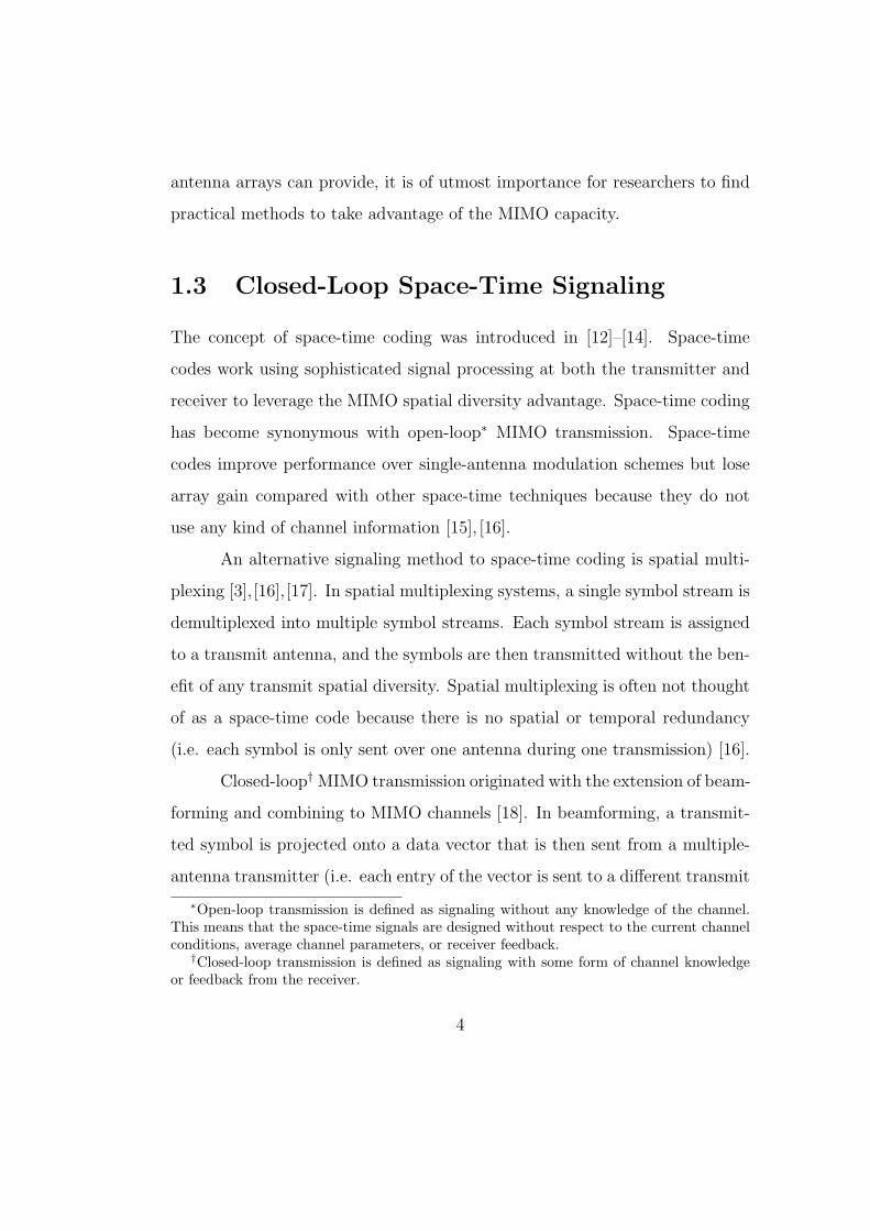
2.2 System Model

A MIMO wireless system with Mt transmit antennas and Mr receive antennas

is shown in Fig. 2.1. An Mt × T matrix X(k) is generated by a coding and

modulation block at transmission k. At time l of the kth transmission, xm,l(k)

is transmitted from the mth transmit antenna.

Coding &

Modulation +

. . . H

. . .

Detection and

Decoding

bits bits X( k ) Y( k )

V( k )

Figure 2.1: Block diagram of a MIMO system.

Assuming optimal pulse-shaping, match-filtering, and sampling, the re-

11

ceived signal matrix for the kth matrix transmission will be modeled as

Y(k) = HX(k) + V(k) (2.1)

where H is an Mr × Mt channel matrix and V(k) is an Mr × T noise ma-

trix. Because of the need to characterize the average performance of a wireless

communication link, the channel matrix H will be modeled as a random ma-

trix [16], [17], [76]. The channel will be modeled as a spatially uncorrelated,

Rayleigh flat fading matrix. This corresponds to a random matrix with inde-

pendent entries each distributed according to CN (0, 1) and assumes sufficient

scattering and the absence of a line-of-sight component. This model assumes

narrowband transmission and sufficiently spaced antennas. The channel is

assumed to follow a block-fading model. With this model, the channel is con-

stant for several blocks of T transmissions and then changes independently to

a new realization. The noise matrix will be modeled as having independent

entries each distributed according to CN (0, N0) where N0 is determined for

the specific system. In general, the N0 variance can be normalized out since

only the signal-to-noise ratio (SNR) is of interest.

After reception, the matrix Y(k) is fed into a decoding and detection

unit where the transmitted signal will be detected. The receiver is assumed

to have perfect knowledge of H. Since the analysis only depends on symbol-

by-symbol detection, the burst index, k, will be omitted to simplify notation.

The matrix X and the decoder to detect the matrix X can take a number of

different forms . For this reason, Sections 2.3-2.6 will overview some common

signaling methods and receiver architectures.

12

2.3 Beamforming

One of the earliest MIMO signaling methods was beamforming. In this method

the matrix X can be written as

X = ws (2.2)

where w ∈ CMt (i.e. T = 1) and s ∈ C. The vector w is called the beamforming

vector while s is a symbol constructed from some constellation S ⊂ C (ex.

binary phase shift keying (BPSK), 4-quadrature amplitude modulation (4-

QAM)). Power is controlled by requiring that Es [|s|2] = Es and w∗w = 1.

Beamforming converts the matrix channel H into an effective vector channel

Hw. The symbol s can then be detected by performing single-dimensional

maximum likelihood (ML) detection on the symbol estimate

z∗Y = z∗Hws + z∗V (2.3)

where z is known as a combining vector. When z = Hw/‖Hw‖2 the combining-

ML receiver corresponds to optimal detection of s.

Note that the vector w must be chosen as a function of the channel in

order to provide any kind of performance benefit. For example, assuming an

optimal combiner,

w = argmaxw∗w=1

‖Hw‖2 (2.4)

in order to minimize the probability of error and maximize the capacity [23],

[26], [37]. This means that beamforming is a closed-loop MIMO signaling

method. Limited feedback methods for beamforming were developed in [18],

[19], [22], [27], [52]–[63].

13

2.4 Spatial Multiplexing

Spatial multiplexing is a capacity-achieving MIMO signaling technique. Tra-

ditional open-loop spatial multiplexing and closed-loop precoded spatial mul-

tiplexing will be discussed.

2.4.1 Open-Loop

In spatial multiplexing, a symbol stream s1, s2, s3, . . . , sMt with si ∈ S for

all i, where S is some constellation, is demultiplexed into a vector X = s =

[s1 s2 . . . sMt ]T [3]. Thus once again, T = 1. The received vector is then

y = Hs + v. (2.5)

Power constraints require that Es [ss∗] = (Es/Mt) IMt so that the transmit

power can be conserved. Note that lower-case letters have been adopted in

this discussion to avoid confusion with the matrix space-time coding techniques

presented later.

Unlike beamforming, spatial multiplexing sends multiple symbols or

multiple substreams at each channel use. This property complicates detec-

tion since the simple linear combining and single-dimensional detection are no

longer optimal. Optimal detection is actually multi-dimensional ML detection

where vectors in SMt are detected rather than symbols in S as was the case

for beamforming [16].

A number of different sub-optimal methods have been proposed for

detection of s. One easily implemented method is the use of a linear receiver.

In this form, the receiver decodes to a vector

s = Q(Gy) (2.6)

14

where G is an Mt×Mr matrix and Q is a function that performs entry-by-entry

ML detection. Note that entry-by-entry ML detection grows linearly with

Mt as opposed to multi-dimensional ML detection which grows exponentially

with Mt. The matrix G can take many forms depending on system needs.

Two methods for choosing G that will be used later are zero-forcing (ZF)

decoding and minimum mean squared error (MMSE) decoding. If ZF decoding

is employed G = H† and if MMSE decoding is employed G = (MN0/EsIMt +

H∗H)−1H∗ [3], [77].

2.4.2 Closed-Loop Precoding

Notice that spatial multiplexing only sends each symbol one time from one

antenna. If one antenna is shadowed, for example, the receiver will lose the

symbol regardless of the form of receive processing because of the lack of

spatial or temporal redundancy. One method for overcoming this problem is

precoding. The basic idea behind precoding is to provide improved diversity

advantage by attempting to send the spatial multiplexing vector only on the

eigen-directions that provide the best performance. When spatial multiplexing

is precoded, X is of the form

X = Fs (2.7)

where F is an Mt ×M matrix with M ≤ Mt. The matrix F can be thought

of as converting the Mt × Mr antenna system into an effective M × Mr an-

tenna system. The symbol vector s is then designed as for an M antenna

transmission. This yields an input/output relation

y = HFs + v (2.8)

15

where F is chosen from some feasible set∗ F . The received vector can then

be decoded just as traditional spatial multiplexing by thinking of HF as an

effective channel.

To date, there have been two different areas of emphasis in closed-

loop spatial multiplexing: MMSE precoding and antenna selection. MMSE

precoding was studied in [28], [29], [78]. The feasible sets considered were

F = {F ∈ CMt×M | λmax{F} ≤ P} (2.9)

or

F = {F ∈ CMt×M | tr (FF∗) ≤ P} (2.10)

where λmax{·} denotes the maximum singular value and P is a power con-

straint. Assuming MMSE linear decoding, a selection criterion is to minimize

the trace or determinant of the mean squared error matrix between the soft

symbol vector estimate Gy and the transmitted vector s [28],[78]. This average

mean squared error matrix is given by

MSE(F) =Es

M

(IM +

Es

MN0

F∗H∗HF

)−1

. (2.11)

The precoder can then be chosen according to

F = argminF′∈F

m(MSE(F′)

)(2.12)

where m(·) is either tr(·) [28], det(·) [28], [29], or a weighted version of the

trace [78]. Note that MMSE precoding assumes an uncountable feasible set

and perfect CSI. The perfect CSI assumption, in particular, makes MMSE

precoding difficult from a practical perspective.

∗A feasible set is the set that a cost function is optimized over.

16

A more practical precoder is antenna selection. In this case F chooses M

out of the Mt antennas to transmit on and turns the other Mt−M antennas off.

Many different criteria have been proposed for antenna selection. To describe

these criteria, assume that the set of possible subsets has been indexed from

1 to(

Mt

M

). Maximum minimum distance antenna selection [79] works well for

ML decoding by choosing the subset index

k = argmax1≤i≤(Mt

M )mins1 6=s2

‖H[i](s1 − s2)‖2 (2.13)

where H[k] is the channel corresponding to signaling on subset k and s1, s2 ∈SM . Maximizing the minimum singular value of HF, λmin{HF}, (see for exam-

ple [71],[79]) has been used to approximately maximize the minimum distance

between codewords for ML decoding and maximize the minimum SNR of over

all substreams for linear receivers. This criterion chooses

k = argmax1≤i≤(Mt

M )λmin{H[i]}. (2.14)

Yet another criterion is to try to maximize the mutual information assuming

an uncorrelated complex Gaussian source [68], [80]. The mutual information

assuming an uncorrelated complex Gaussian source given subset choice H[k] is

I(H[k]) = log2 det

(IM +

Es

MN0

H∗[k]H[k]

). (2.15)

Therefore a capacity inspired selection criterion is given by

k = argmax1≤i≤(Mt

M )I(H[i]). (2.16)

The only previously proposed closed-loop precoding methods that can

be directly implemented in systems without transmit channel knowledge are

17

the antenna selection precoders. Antenna selection is always a limited feedback

system because there are only(

Mt

M

)ways to choose M antenna subsets from

Mt antennas so F can be conveyed from the receiver to the transmitter using⌈log2

(Mt

M

)⌉bits.

Unfortunately, antenna selection suffers in performance when compared

with the unconstrained precoders (see for example the simulations in [72],[73]).

One of the objectives of this dissertation is to extend the concepts and benefits

of antenna selection to limited feedback, unconstrained precoders. This would

allow the limited feedback system to use any number of bits of feedback rather

than simply⌈log2

(Mt

M

)⌉and benefit from the increased array gain available

with more feedback.

Example: An example of the performance degradation on a 5×4 system

using 4-QAM and four substreams is presented in Fig. 2.2. Antenna selection

using the minimum singular value with a ZF decoder and MMSE precoding

are plotted along with 4 × 4 spatial multiplexing using ZF and ML decod-

ing. MMSE with the determinant cost function outperforms antenna selection

by 1.3dB. As well MMSE with the trace cost function outperforms antenna

selection by approximately 1.7dB.

2.5 Orthogonal Space-Time Block Coding

OTSBCs were some of the first proposed space-time block codes [13],[14]. The

following discussion will overview OSTBCs for use in open-loop and closed-loop

systems. The explanation of OSTBCs will follow from the linear dispersion

formulation taken from [81].

18

−2 0 2 4 6 8 10 1210

−3

10−2

10−1

100

Eb/N

0

Pro

babi

lity

of S

ymbo

l Vec

tor

Err

or

No Precoding(4×4 ZF)No Precoding(4×4 ML)Ant Select(ZF)MMSE (det)MMSE (tr)

Figure 2.2: Probability of error comparison of antenna selection and MMSEprecoding.

2.5.1 Open-Loop

An OSTBC codeword is created from a set of ns symbols s1, s2, . . . , sns all

taken from the same constellation S ⊂ C. An Mt × T codeword is formulated

as

X =ns∑i=1

(siAi + s∗i Bi) (2.17)

where Ai and Bi for all i are matrices that satisfy several orthogonality prop-

erties [16]. Note that for OSTBCs, T > 1. Because of the power constraint

properties,

XX∗ =

(ns∑i=1

|si|2)

IMt (2.18)

[16]. For power constraint reasons, it is assumed that Esi[|si|2] = Es/Mt.

The orthogonality properties allow the received matrix Y to have a

19

simple linear decoding structure [13], [14]. They also allow for a simple upper

bound on the probability of error [12], [43], [45],

Pr(ERROR) ≤ e−γ‖H‖2F (2.19)

where γ is a constant scale factor that is a function of S and Mt. Because γ

is constant, the performance of OSTBC is thus a decreasing function of the

channel power ‖H‖F .

2.5.2 Closed-Loop Precoding

Closed-loop OSTBC using precoding was studied in [42]–[49]. When precoding

is employed,

X = FC (2.20)

where F is an Mt×M matrix chosen from a feasible set F and C is an M ×T

OSTBC codeword. Thus the OSTBC will be designed as if it were being sent

over M transmit antenna.

Current work in precoded OSTBCs has used a selection criterion for F

that minimizes (2.19) using an effective channel HF [42]–[49]. Thus, minimiz-

ing (2.19) is equivalent to maximizing ‖HF‖F , so F can be chosen by

F = argmaxF′∈F

‖HF′‖F . (2.21)

Various feasible sets for F have been considered. The restriction of F to

diagonal matrices with a trace constraint was studied in [48], [49]. Note that

this method is not a limited feedback method because F is uncountable. The

authors in [42]–[44], [46] consider precoders where M = Mt and

F = {F ∈ CMt×M | ‖F‖2F ≤ M}. (2.22)

20

All of these precoding techniques lead to uncountable F . Antenna selection

uses a finite feasible set and chooses the antenna subset k such that

k = argmax1≤i≤(Mt

M )‖H[i]‖F . (2.23)

Only two of these approaches work when the transmitter has no CSI.

Once again, antenna selection is a limited feedback system because the subset

chosen can be conveyed from receiver to transmitter using⌈log2

(Mt

M

)⌉bits. A

limited feedback method was proposed in [44], [46] by requiring the receiver to

convey a quantized version of the channel, Hquant, using a limited number of

bits to the transmitter. With this approach F is chosen from

F = argmaxF′∈F

‖HquantF′‖F . (2.24)

Unfortunately a design method for constructing a quantized feasible set

(i.e. finite card(F)) other than antenna selection has not yet been derived. The

limited feedback unconstrained precoders using a quantized channel are not

easily implemented and require difficult optimizations [44],[46]. Therefore, one

of the main objectives of the proposed research is to understand how quantized

feasible sets for precoded OSTBCs should be designed. Solving this problem

will convert the difficult optimizations in [44], [46] a simple brute force search

over the codebook matrices.

2.6 Diversity-Multiplexing Tradeoff

A simple characterization of space-time systems is their diversity-multiplexing

tradeoff [36]. The parameters of diversity and multiplexing have precise mathe-

matical definitions. A system is said to have diversity gain (also called diversity

21

order) of d if

d = − limEs/N0→∞

log (Pr(ERROR))

log (Es/N0). (2.25)

A system has a multiplexing gain of r if the supported data rate satisfies

R(Es/N0) ≈ r log2(Es/N0) (2.26)

where R(Es/N0) is the rate supported when the SNR is Es/N0.

These two parameters can fundamentally characterize the performance

of a MIMO signaling scheme [36]. Spatial multiplexing, for example, achieves

maximum multiplexing gain [3], while OSTBC achieves maximum diversity

gain [13], [14]. Space-time block codes have been designed that tradeoff the

two gains (see for example codes designed from [81]), but a simple tradeoff can

be made using closed-loop MIMO techniques [39].

The basic idea behind [39] is to fix the rate of the signaling scheme

per channel use and then to choose spatial multiplexing when dmin,SM >

dmin,OSTBC and to choose OTSBC when dmin,SM < dmin,OSTBC where dmin,SM

is the received minimum distance of spatial multiplexing and dmin,OSTBC is the

received minimum distance for an OSTBC. This method achieves the maxi-

mum diversity gain [39] and can be easily implemented using 1 bit of feedback.

Unfortunately, OSTBCs suffer from a rate loss for Mt > 2 for all constellations

except pulse amplitude modulation (PAM) and have design methods that do

not easily generalize to arbitrary Mt [14]. Therefore, a generalized method

of [39] that is not dependent on OSTBCs is of practical interest.

22

Chapter 3

Limited Feedback Precoding for

Space-Time Codes

This chapter proposes a limited feedback framework for precoded orthogonal

space-time block codes. The chapter is organized as follows. Section 3.1

provides a general overview of the system under consideration. A selection

criterion for limited feedback OSTBC precoding is derived in Section 3.2. The

codebook design problem is solved in Section 3.3. Section 3.4 shows that the

designed codebooks provide full diversity order in Rayleigh fading channels.

We present Monte Carlo simulation results in Section 3.5.

3.1 System Overview

An Mt transmit antenna and Mr receive antenna limited feedback precoded

OSTBC system is illustrated in Fig. 3.1. A block of ns symbols s1, s2, . . . , sns

c© 2004 IEEE. Reprinted, with permission, from D. J. Love and R. W. Heath Jr.,“Limited Feedback Unitary Precoding for Orthogonal Space-Time Block Codes,” acceptedto IEEE Transactions on Signal Processing.

23

OSTBC Encoder

symbol stream

Decouple Symbols

& ML

Decoding hMr,1

h1,2

x1,t

x2,t

xMt,t

y1,t

y2,t

yMr,t

wMr,t

w2,t

w1,t

C

F

X

symbol stream

Select F from F using binary index

Choose F from F Send binary codebook index

• • •

• • •

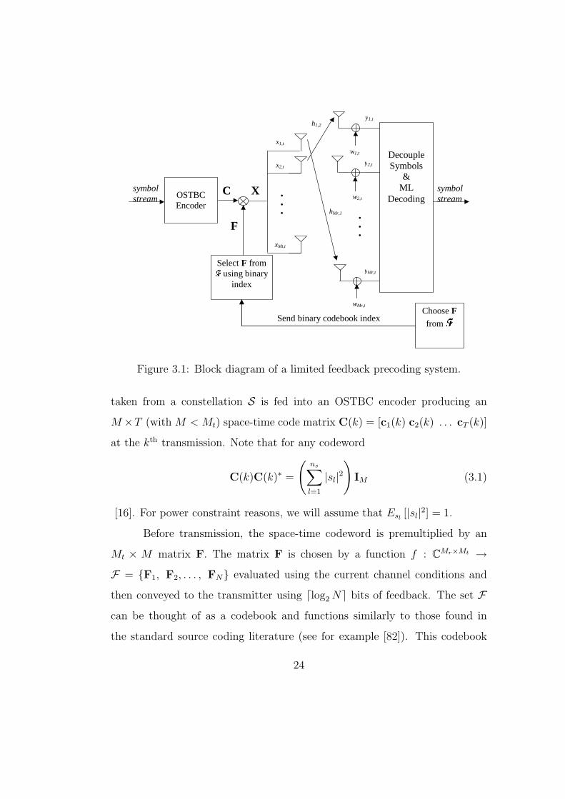
Figure 3.1: Block diagram of a limited feedback precoding system.

taken from a constellation S is fed into an OSTBC encoder producing an

M×T (with M < Mt) space-time code matrix C(k) = [c1(k) c2(k) . . . cT (k)]

at the kth transmission. Note that for any codeword

C(k)C(k)∗ =

(ns∑

l=1

|sl|2)

IM (3.1)

[16]. For power constraint reasons, we will assume that Esl[|sl|2] = 1.

Before transmission, the space-time codeword is premultiplied by an

Mt × M matrix F. The matrix F is chosen by a function f : CMr×Mt →F = {F1, F2, . . . , FN} evaluated using the current channel conditions and

then conveyed to the transmitter using dlog2 Ne bits of feedback. The set Fcan be thought of as a codebook and functions similarly to those found in

the standard source coding literature (see for example [82]). This codebook

24

is designed offline and known to both the transmitter and receiver. We will

impose a peak power limit for all F ∈ F by requiring that

maxs∈SM

‖Fs‖2

‖s‖2

≤ 1

for any constellation S ⊆ C. Because S is non-empty and 0 /∈ S, this constraint

corresponds to the assumption that λ1{F} ≤ 1 for all F ∈ F . We will further

restrict the form of the matrices in F , but the justification will be presented

in Section 3.2.

We assume that the transfer function between the transmitter and re-

ceiver can be modeled as a spatially uncorrelated, memoryless linear chan-

nel that is constant over several codeword transmissions before independently

taking on a new value. Assuming optimal pulse shaping, match-filtering, and

sampling, the received signal can thus be written as

Y =

√ρ

MHFC + W (3.2)

where H is the Mr ×Mt channel matrix with independent entries distributed

as CN (0, 1), W is an Mr×T noise matrix with independent entries distributed

according to CN (0, 1), and ρ is the signal-to-noise ratio (SNR). F corresponds

to the evaluation of the mapping function for the current channel realization

H, i.e.

F = f(H).

Note that we have suppressed the temporal parameter k in C(k) because of

our channel model and interest in the use of codeword-by-codeword detection.

After reception, the receiver performs maximum likelihood (ML) decoding on

the OSTBC using the received matrix Y and the effective channel HF.

25

Problem Statement: Given a system illustrated by Fig. 3.1 and

described by (3.2), two main problems arise. The first problem we address

is the selection of an optimal precoder for given channel from a codebook of

matrices F . The second problem is how to design the set F given the chosen

selection criterion. Solving these problems is the objective of this chapter.

3.2 Selection Criterion

The first issue with limited feedback unitary precoding we address is the

design of the precoder selection mapping f(·). We assume an arbitrary set

F ⊂ L(Mt,M) and ML decoding.

Our goal in this chapter is to minimize the symbol error rate (SER)

given H, P r(ERROR | H). Closed-form expressions for the SER would be

extremely difficult to obtain because they would be a function of the effec-

tive channel HF that is in general no longer matrix Rayleigh fading and the

selection function f(·).We will therefore take the approach of [14], [42], [43], [45] and will use

a bound on the probability of error. Using the ML detection properties of

OSTBCs, it can be shown that

Pr(ERROR | H) ≤ exp(−γ‖HF‖2

F

)(3.3)

where γ is a function that depends on M, ρ, and S [16]. Because γ is fixed,

minimizing the bound in (3.3) requires the maximization of ‖HF‖F . Note that

this maximization is equivalent to choosing the matrix F ∈ F that maximizes

the receive minimum distance

dmin = minCk 6=Cl

‖HF (Ck −Cl)‖F (3.4)

26

because of the orthogonality of the OSTBC codewords in (3.1). Therefore, we

can state the following selection criterion:

Selection Criterion: Choose the limited feedback precoder according to

F = f(H) = argmaxF′∈F

‖HF′‖F . (3.5)

This selection criterion can be implemented by computing a matrix

multiplication and Frobenius norm for each of the N codebook matrices. Ties

in distance between codeword matrices are broken arbitrarily by selecting the

precoding matrix with the lowest index because they occur with zero proba-

bility.

To bound the performance with quantized precoding, it is of interest

to characterize an optimal unquantized precoder over the set L(Mt, M). Note

that this matrix Fopt will not be unique over L(Mt, M) because for any U ∈U(M, M), ‖HFopt‖F = ‖HFoptU‖F . Let the singular value decomposition of

H be given by

H = VLΣV∗R (3.6)

where VL ∈ U(Mr,Mr), VR ∈ U(Mt,Mt), and Σ is an Mr × Mt diagonal

matrix with λi{H} at entry (i, i). Let VR be the matrix formed from the

first M columns of VR. The following lemma shows an optimal matrix in this

unquantized scenario.

Lemma 1 An optimal unquantized precoder Fopt over L(Mt,M) that maxi-

mizes ‖HFopt‖F is given by Fopt = VR.

Proof Let F have singular value decomposition F = ULΓU∗R where UL ∈

U(Mt,Mt), UR ∈ U(M,M), and Γ is an Mt×M diagonal matrix with λi{F}

27

at entry (i, i). It then follows that

‖HF‖F = ‖ΣV∗RULΓ‖F (3.7)

≤∥∥∥ΣV∗

RUL [IM 0]T∥∥∥

F

≤

√√√√M∑i=1

λi{U∗LVRΣTΣV∗

RUL}

=∥∥Σ

∥∥F

. (3.8)

by using the invariance of the Frobenius norm to unitary transformation [83]

in (3.7) and the singular values bounds of F where 0 is M × (Mt−M) matrix

of zeros and Σ is the matrix consisting of the first M columns of Σ. Equality

in (3.8) is obtained when F = VR.

Lemma 1 is interesting because it says that not only is λ1{Fopt} = 1

but λi{Fopt} = 1 for 1 ≤ i ≤ M. Intuitively, this means that we should always

transmit at full power on the precoder effective channel modes when perform-

ing optimal precoding. This result would be expected given the mean squared

error results for precoded spatial multiplexing in [28]. We are, however, in-

terested in sub-optimal precoders constructed using a limited feedback path.

The following lemma shows that all precoding matrices should have full power

in the singular values.

Lemma 2 If F ∈ L(Mt,M) has a singular value decomposition F = ULΓU∗R

and λM{F} < 1, then F = UL[IM 0]T satisfies ‖HF‖F < ‖HF‖F .

Proof Assume F has a singular value decomposition as shown in the first

lemma. Then

‖HF‖F = ‖HULΓ‖F < ‖HUL[IM 0]T‖F = ‖HF‖F

28

using the invariance of the Frobenius norm to unitary transformation [83], the

singular value bound for F, and F = UL[IM 0]T .

Lemma 2 demonstrates the significant effect that the power restriction

has on optimal precoders. The sum power constraint results in [28], [47], [78]

all yield optimal precoders with unequal power allocation among the precoder

singular values. In contrast, unequal power pouring when using a maximum

singular value constraint only reduces the total transmit power.

Lemma 2 reveals that the precoder should always be designed to have

singular values that are as large as possible. Because of the maximum singular

value restriction, the precoder should be chosen from the set U(Mt,M) rather

than L(Mt,M). For this reason we will restrict F ⊂ U(Mt, M) and thus only

design our precoders over U(Mt,M).

3.3 Chordal Distance Precoding: Motivation

and Codebook Design

In this section, we derive a codebook design criterion that follows directly

from the Section 3.2 codeword selection result. This criterion is based on a

distortion function that we define in order to minimize the average SER. The

criterion turns out to relate to the famous applied mathematics problem of

Grassmannian subspace packing.

3.3.1 Distortion Function

To design a codebook we will propose a distortion measure that is a function of

the channel and then find a codebook that minimizes the average distortion.

29

This distortion function must differ, however, from the distortion functions

commonly used in vector quantization such as mean squared error (see for ex-

ample [82]) because we are interested in improving system performance rather

than improving the quality of the estimated precoder at the transmitter.

Essentially, we would like the quantized equivalent channel HF to pro-

vide SER performance close in some sense to that provided by the optimal

precoded equivalent channel HFopt where F ∈ F is the “best” precoding ma-

trix in the codebook. Along these lines, consider the total effective power

‖HF‖2F , which according to (3.3) relates to the SER. The loss in received

channel power is expressed as

minF′∈F

(‖HFopt‖2F − ‖HF′‖2

F

). (3.9)

We propose to design the codebook by considering, as a measure of distortion,

the average of the loss in received channel power given by

EH

[minF′∈F

(‖HFopt‖2F − ‖HF′‖2

F

)]. (3.10)

Recall that ‖HFopt‖F ≥ ‖HF‖F for all F ∈ U(Mt,M) so the function will

always be nonnegative. Notice also that minimizing this distortion function

relates directly to minimizing the bound on the SER in (3.3). Thus the distor-

tion has physical meaning in terms of the SER, as opposed to a mean squared

error distance function.

The distortion function in (3.10) yields little insight into the codebook

design problem directly, thus we will derive a tight upper bound on the distor-

tion. Using Lemma 1 and the definition of Σ, the distortion for this arbitrary

30

matrix is written as

minF′∈F

(‖HFopt‖2F − ‖HF′‖2

F

)

= minF′∈F

(tr

(ΣΣ

T)− tr

(ΣV∗

RF′F′∗VRΣT))

≤ minF′∈F

(tr

(ΣΣ

T)− tr

(ΣV

∗RF′F′∗VRΣ

T))

(3.11)

= minF′∈F

tr(Σ

TΣ

(IM −V

∗RF′F′∗VR

))(3.12)

≤ λ21{H}min

F′∈Ftr

(IM −V

∗RF′F′∗VR

)(3.13)

= λ21{H}min

F′∈F1

2

∥∥∥VRV∗R − F′F′∗

∥∥∥2

F(3.14)

where (3.11) follows from zeroing the least Mt−M singular values of H, (3.13)

follows by substituting λ1{H} for the other non-zero singular values in (3.12),

and (3.14) uses the alternative representation for subspace distance [84].

To find a good codebook for many channel realizations, we are interested

in the average distortion of our codebook given by

EH

[minF′∈F

(‖HFopt‖2F − ‖HF′‖2

F

)]. (3.15)

Using (3.14) and the independence of Σ and VR [85],

EH

[minF′∈F

(‖HFopt‖2F − ‖HF′‖2

F

)]

≤ EH

[λ2

1{H}]EH

[minF′∈F

1

2

∥∥∥VRV∗R − F′F′∗

∥∥∥2

F

]. (3.16)

Thus by bounding the distortion function we can think of the limited feedback

performance as being characterized by two different terms, one related to the

distribution of the maximum channel singular value and another representing

the “quality” of the codebook F .

31

3.3.2 Codebook Design Criterion

Minimizing (3.16) requires finding the distribution of VR. Recall that a matrix

V is isotropically distributed on U(Mt,M) if for any Θ ∈ U(Mt,Mt), Θ∗V d=

V withd= denoting equivalence in distribution [86]. The following lemma gives

this distribution.

Lemma 3 The optimal precoding matrix Fopt = VR for a memoryless, i.i.d.

Rayleigh channel H is isotropically distributed on U(Mt,M).

Proof First note that Fopt = VR = VR[IM 0]T . Since VR is isotropically

distributed [85], it is easily seen that Θ∗Foptd= Fopt.

To propose a design for F , let us review some common properties of

finite subsets of U(Mt,M). These properties are found in the Grassmannian

subspace packing literature (for example [84], [87]–[90]). The set U(Mt,M)

defines the Stiefel manifold [90]. Each matrix in U(Mt,M) generates an

M -dimensional subspace of the complex Mt-dimensional vector space CMt .

We will adopt Grassmannian packing notation and define the set of all column

spaces of the matrices in U(Mt,M) to be the complex Grassmann manifold

G(Mt,M). Thus if F1,F2 ∈ U(Mt,M) then the column spaces of F1 and F2,

PF1 and PF2 respectively, are contained in G(Mt,M). A normalized invari-

ant measure µ is induced on G(Mt,M) by the Haar measure on U(Mt,M).

This measure allows the computation of volumes within G(Mt,M). Subspaces

within the Grassmann manifold can be related by their distance from each

other. The chordal distance between the two subspaces PF1 and PF2 is given

by

d(F1,F2) =1√2‖F1F

∗1 − F2F

∗2‖F . (3.17)

32

Let V = {PF1 ,PF2 , . . . ,PFN} be the set of column spaces where PFk

is

the column space of Fk. This set V ⊂ G(Mt,M) is a packing of subspaces in

G(Mt,M). A packing can be described by its minimum distance

δ = min1≤k<l≤N

d(Fk,Fl). (3.18)

The Grassmannian subspace packing problem is the problem of finding the set

of N subspaces in G(Mt,M) such that δ is as large as possible.

Consider the open ball in G(Mt,M) of radius δ/2 defined as

BFk(δ/2) = {PU ∈ G(Mt,M) | d(U,Fk) < δ/2}. (3.19)

Notice that the balls are disjoint by the triangle inequality of metrics [84]. This

observation allows the density of a chordal subspace packing to be defined as

∆(F) = µ

(N⋃

k=1

BFk(δ/2)

)=

N∑

k=1

µ (BFk(δ/2)) . (3.20)

Using the density, we find the probability of the isotropically distributed

VR falling in one of the sets BFk(δ/2) can be expressed as

Pr

(VR ∈

N⋃

k=1

BFk(δ/2)

)= ∆(F). (3.21)

For large Mt, it has been shown in [84] that

∆(F) ≈ N

(δ

2√

M

)2MtM+o(Mt)

. (3.22)

We can thus bound the “codebook quality” term in (3.16) as

EH

[minF′∈F

1

2

∥∥∥VRV∗R − F′F′∗

∥∥∥2

F

]

≤ 1

4δ2∆(F) + M(1−∆(F))

≈ M + N

(δ

2√

M

)2MtM+o(Mt) (1

4δ2 −M

). (3.23)

33

Differentiating (3.23) and noting δ <√

M easily shows that the bound is a

decreasing function of δ when 2MtM + o(Mt) > 2/3. We know from the prob-

abilistic analysis in [59] that this is always satisfied for any Mt when M = 1

because o(Mt) = −2. As well, we also know that this assumption is also sat-

isfied for large Mt because of the definition of the little-o Landau symbol. We

have experimentally verified this assumption for many other M and conjecture

that it is always true. Thus practically (3.23) is minimized by maximizing δ.

We have now established that designing low distortion codebooks is equivalent

to packing subspaces in the Grassmann manifold using the chordal distance

metric.

Therefore we now understand how to design codebooks for limited feed-

back precoding. Maximizing the minimum subspace distance between any pair

of codebook column spaces approximately minimizes our distortion bound.

Thus, we state the following design method for creating limited feedback pre-

coding codebooks.

Codebook Design Summary: The codebook F = {F1, F2, . . . , FN} should

be designed such that δ = min1≤k<l≤N d(Fk,Fl) is as large as possible.

3.3.3 Practical Codebook Designs

Finding good precoder codebooks from Grassmannian packings for arbitrary

Mt, M, and N is actually quite difficult [87]–[89]. For instance, in the simplest

case of M = 1 where the Rankin lower bound on line packing correlation [89]

can be employed, packings that achieve equality with the lower bound are

often impossible to design. A comprehensive tabulation of real packings can

be found on [91]. The most practical method for generating these packings

34

is to use codebooks designed from the non-coherent space-time modulation

designs in [87] and [92].

The search algorithm in [92] can be very easily implemented and yields

codebooks with large minimum distances. The algorithm works by considering

codebooks of the form

F = {FDFT , ΘFDFT , . . . , ΘN−1FDFT}

where FDFT is an Mt ×M matrix with 1√Mt

ej 2π

Mtkl

at entry (k, l) and Θ is a

diagonal matrix given by

Θ =

ej 2πN

u1 0 · · · 0

0 ej 2πN

u2 · · · 0...

. . ....

0 0 · · · ej 2πN

uMt

where

0 ≤ u1, . . . , uMt ≤ N − 1.

The values for u1, u2, . . . , uMt are chosen according to the entries of the vector

u = [u1 u2 · · · uMt ]T from the set Z = {u ∈ ZMt | ∀k, 0 ≤ uk ≤ N − 1}

given by

u = argmaxZ

min1≤l≤N−1

d(FDFT ,ΘlFDFT ).

Thus, there are NMt different possibilities for Θ that must be checked.

For small transmit antenna arrays and/or low feedback rates, it is possible to

search over all possible values of u in Z. In general, however, random search

methods must be employed to design F . These methods optimize the cost

function by randomly testing values of u using a uniform distribution on Z.

35

Codebooks designed from [92] also have the added benefit of easy mem-

ory storage. The codebook F can be stored at the transmitter/receiver using

dMt log2 Ne bits because only the numbers u1, u2, . . . , uMt need to be stored.

The chosen codeword matrix F can then be easily calculated by computing

Θl−1FDFT for the chosen binary codeword index l. Note that the matrix FDFT

can be either stored or computed at each codebook update.

3.4 Performance Analysis

Because of the difficulty in deriving closed-form SER expressions, we will char-

acterize the diversity of our limited feedback precoders. A signaling scheme is

said to obtain diversity order d if [36]

d = − limρ→∞

log Pr(ERROR)

log ρ.

We can bound the asymptotic performance of limited feedback precoding

given a channel using the SER bound in (3.3). Thus in order to under-

stand the diversity performance of limited feedback precoding, we will bound

maxF′∈F ‖HF′‖F .

It follows from the Poincare separation theorem [83], pp. 190 that

maxF′∈F

‖HF′‖F ≤ ‖H‖F .

Note that ‖H‖F is the post-processing channel gain of an Mt antenna OSTBC

that is known to obtain a diversity order of MtMr [14]. Therefore, the diversity

order of our limited feedback precoders is less than or equal to MtMr. Thus

all that is needed is a lower bound on diversity order.

Let fk,l denote the lth column of codebook matrix Fk. The following

lemma will prove useful in lower bounding maxF′∈F ‖HF′‖F .

36

Lemma 4 Let F = {F1, F2, . . . , FN} be a codebook with packing minimum

distance δ and N ≥ Mt/M. If there exists a vector v ∈ CMt such that F∗kv = 0

for all 1 ≤ k ≤ N, then

1.) There exists (k′, l′) such that fk′,l′ =∑m

i=1 αifki,li where ki and li are index-

ing sequences with (ki, li) 6= (k′, l′), 0 < |αi| < 1, and 1 ≤ m < Mt,

2.) A new codebook F with

fk,l =

fk,l if (k, l) 6= (k′, l′);

v if (k, l) = (k′, l′)

has minimum distance δ ≥ δ.

Proof Part 1 follows from the fact that a basis for the column space of the

matrix E =[F1 F2 · · · FN

]can be formed from m < Mt columns of the

matrix E. Part 2 is a result of the fact that for k 6= k′, ‖F∗kFk′‖F = ‖F∗kFk′‖F ≥‖F∗kFk′‖F where

Fk′ = [fk′,1 · · · fk′,l′−1 v fk′,l′+1 · · · fk′,M ].

By applying Lemma 4 repeatedly, any N ≥ Mt/M matrix codebook

F with minimum distance δ and columns {fk,l} that do not span CMt can be

trivially modified to a codebook F with columns {fk,l} that span CMt and

minimum distance δ ≥ δ. Therefore we can state the following theorem.

Theorem 1 If N ≥ Mt/M and the columns {fk,l} span CMt , then F =

{F1, F2, . . . , FN} provides full diversity order.

37

Proof First note that the channel power is given by maxF′∈F ‖HF′‖2F . Notice

that

maxF′∈F

‖HF′‖2F ≥ max

k,l‖Hf ′k,l‖2

2

≥ 1

Mr

maxk,l

‖Hf ′k,l‖21

=1

Mr

‖HE‖21

where E = [F1 F2 · · · FN ] . Because the columns {fk,l} span CMt , we can

find UE,L ∈ U(Mt,Mt), UE,R ∈ U(NM, NM), and Φ with diagonal entries

φ1 ≥ φ2 ≥ . . . ≥ φMt > 0 such that E = UE,LΦU∗E,R. Then using the

invariance of complex normal matrices to unitary transformation [85] and the

bounds in [59],

maxF′∈F

‖HF′‖2F

d= max

F′∈F‖HU∗

E,LF′‖2

F

≥ 1

NMMr

‖HΦ‖21

≥ φ2Mt

NMMr

‖H‖21

≥ φ2Mt

NMM2t Mr

‖H‖2F

The lower boundφ2

Mt

NMM2t Mr

‖H‖2F is the channel gain of an Mt antenna OSTBC

with an array gain shiftφ2

Mt

NMM2t Mr

. Systems with effective channel gains of this

form are known to obtain a diversity order of MtMr [14]. We can conclude

now that the limited feedback precoders designed using the chordal distance

obtain full diversity order.

Because limited feedback precoding maintains full diversity performance,

this allows the generalization of OSTBCs to transmission over any transmit

38

antenna configuration with full diversity. This lemma generalizes the result

in [45] that proves antenna selection achieves full diversity order.

3.5 Simulations

Precoded OSTBCs using chordal distance limited feedback precoders have

been simulated in the following experiments. The precoder codebooks were

designed using the criterion proposed in Section 3.3 and implemented with

packings designed from [92]. For comparison, OSTBCs with antenna selection

have also been simulated [45].

Note that by our power scaling definitions, ρ is the ratio of the total

transmitted energy to noise power for each transmission. For example, if a

two antenna Alamouti code were transmitted then

X =

√ρ

2F

s1 s∗2

s2 −s∗1

with Es1

[|s1|2]

= Es2

[|s2|2]

= 1.

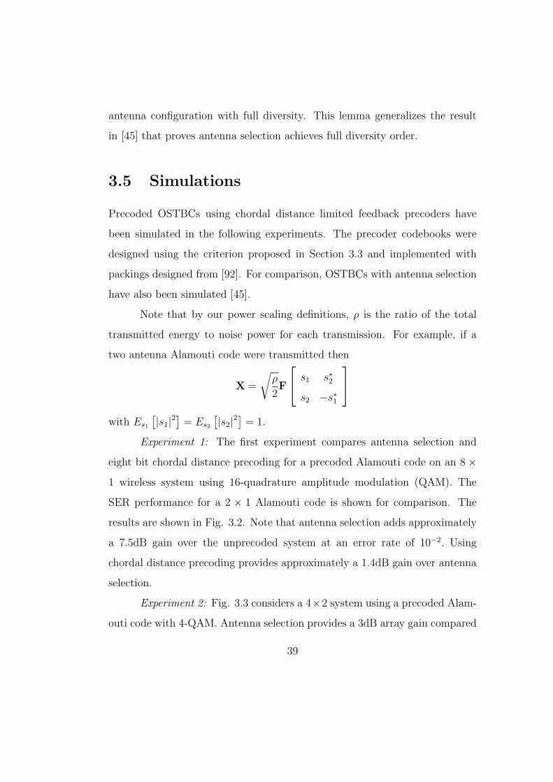
Experiment 1: The first experiment compares antenna selection and

eight bit chordal distance precoding for a precoded Alamouti code on an 8 ×1 wireless system using 16-quadrature amplitude modulation (QAM). The

SER performance for a 2 × 1 Alamouti code is shown for comparison. The

results are shown in Fig. 3.2. Note that antenna selection adds approximately

a 7.5dB gain over the unprecoded system at an error rate of 10−2. Using

chordal distance precoding provides approximately a 1.4dB gain over antenna

selection.

Experiment 2: Fig. 3.3 considers a 4×2 system using a precoded Alam-

outi code with 4-QAM. Antenna selection provides a 3dB array gain compared

39

4 6 8 10 12 14 16 18 20 22 24 2610

−4

10−3

10−2

10−1

100

ρ (dB)

Pro

babi

lity

of S

ymbo

l Err

or

No Precoding(2×1)Ant SelectGrass 8Bit

Figure 3.2: SER comparison of various OSTBC precoding schemes for a twosubstream 8× 1 system using 16-QAM.

with an unprecoded OSTBC. Chordal distance precoding with a three bit code-

book provides over a 0.3dB array gain and with a six bit codebook provides

over a 0.7dB array gain over antenna selection. Interestingly, antenna selection

requires⌈log2

(42

)⌉= 3 bits of feedback. Thus, by simply lifting the restriction

of F having columns of IMt adds a 0.3dB gain.

Experiment 3: The third experiment addresses the performance of a

5× 4 wireless system using the OSTBC

C =

s1 0 s2 −s3

0 s1 s∗3 s∗2

−s∗2 −s3 s∗1 0

(3.24)

obtained from [16] with 16-QAM. The results are shown in Fig. 3.4. Using

antenna selection adds around a 1.5dB improvement over a 3× 4 OSTBC. An

40

0 2 4 6 8 10 12 14

10−3

10−2

10−1

ρ (dB)

Pro

babi

lity

of S

ymbo

l Err

or

No Precoding(2×2)Ant SelectGrass 3BitGrass 6Bit

Figure 3.3: SER comparison of various OSTBC precoding schemes for a twosubstream 4× 2 system using 4-QAM.

array gain of approximately 0.4dB is added by using six bit chordal distance

precoding instead of antenna selection. Chordal distance precoding with an

eight bit codebook outperforms antenna selection by more than 0.5dB.

Experiment 4: The fourth experiment, shown in Fig. 3.5, addresses the

performance of a precoded OSTBC using the code in (3.24) over a 6×3 wireless

with 16-QAM. Six and eight bit chordal distance precoding have array gains of

approximately 2.1dB and 2.3dB, respectively, compared to unprecoded 3 × 3

OSTBCs. Note that six bits provides most of the array gain available with

eight bits, thus a careful simulation analysis must be done in any practical

system before choosing a given feedback rate.

Experiment 5: The effect of channel estimation error during precoder

selection for an 8 × 1 Alamouti system is addressed in Fig. 3.6. Antenna

41

4 5 6 7 8 9 10 11 12 13 14 15

10−3

10−2

10−1

ρ (dB)

Pro

babi

lity

of S

ymbo

l Err

or

No Precoding(3×4)Ant SelectGrass 6BitGrass 8Bit

Figure 3.4: SER comparison of various OSTBC precoding schemes for a threesubstream 5× 4 system using 16-QAM.

selection and eight bit chordal distance precoding are simulated for various

channel correlations. We simulate estimation error by assuming that the re-

ceiver chooses F = f (Hest) using knowledge of a matrix Hest where

Hest = αH +√

1− α2Herror (3.25)

where the entries of Herror are independent and distributed according to

CN (0, 1). Notice that by our definition for α this means E[vec(Hest)vec(H)∗] =

αIMrMt . Note that Hest is a biased estimate of H. This is to emphasize that

the channel estimate is not only a noisy estimate but also a dated estimate.

Thus the precoder was designed based on an outdated channel estimate.

It is assumed that the ML decoder has perfect knowledge of HF in or-

der to isolate the effect of precoder mismatch. Interestingly, eight bit chordal

distance precoding still outperforms perfect channel knowledge antenna subset

42

4 6 8 10 12 14 16

10−3

10−2

10−1

ρ (dB)

Pro

babi

lity

of S

ymbo

l Err

or

No Precoding(3×3)Grass 6BitGrass 8Bit

Figure 3.5: SER comparison of various OSTBC precoding schemes for a threesubstream 6× 3 system using 16-QAM.

selection for α2 = 0.9. When α2 = 0.75, chordal distance precoding performs

approximately the same as α2 = 0.9 antenna selection. This result demon-

strates that chordal distance precoding allows a tradeoff between the quality

of the channel estimation and the rate of the feedback path. At the expense

of requiring more feedback, limited feedback chordal distance precoding can

obtain a lower probability of error than antenna selection even in the presence

of channel estimation error.

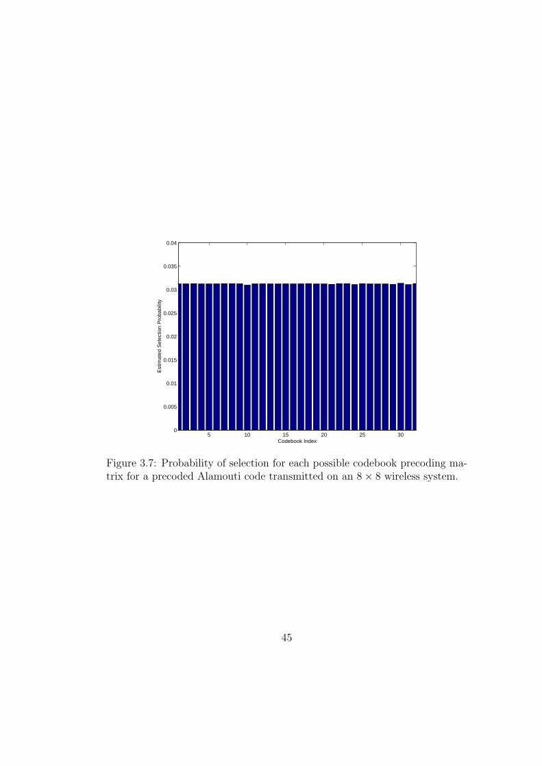
Experiment 6: The final experiment validates that the codebooks achieve

the entropy lower bound on codeword bit length [93], pp. 86. In this exper-

iment, an 8 × 8 wireless system transmitting a precoded Alamouti code was

simulated in order to estimate the probability that each codeword precoder is

selected. A five bit codebook was simulated. The results are shown in Fig.

43

4 6 8 10 12 14 16 18 20 22

10−3

10−2

10−1

100

ρ (dB)

Pro

babi

lity

of S

ymbo

l Err

or

Ant Select(α=1)Ant Select(α2=0.9)Ant Select(α2=0.75)Grass 8Bit(α2=1)Grass 8Bit(α2=0.9)Grass 8Bit(α2=0.75)

Figure 3.6: SER comparison of various OSTBC precoding schemes with chan-nel estimation error for a two substream 8× 1 system using 16-QAM.

3.7. Note that a uniform distribution across the codebook would mean that

each matrix is selected with probability 1/25 = 0.03125. All estimated selec-

tion probabilities are within 2.5 × 10−4 of the uniform selection probability.

Thus the precoder matrix to be encoded, F = f(H), has an entropy of

25∑j=1

2−5 log2(25) = 5 bits.

An optimal data compression algorithm to encode the precoder matrix F can

at best achieve an average codeword bit length of five bits. Because we transmit

each precoder codeword with log2 N = 5 bits, our codebook has been experi-

mentally shown to obtain the optimal codeword bit length lower bound [93].

44

5 10 15 20 25 300

0.005

0.01

0.015

0.02

0.025

0.03

0.035

0.04

Codebook Index

Est

imat

ed S

elec

tion

Pro

babi

lity

Figure 3.7: Probability of selection for each possible codebook precoding ma-trix for a precoded Alamouti code transmitted on an 8× 8 wireless system.

45

Chapter 4

Limited Feedback Precoding for

Spatial Multiplexing

In this chapter, a limited feedback framework for precoded spatial multiplex-

ing is discussed. This chapter is organized as follows. Section 4.1 reviews

the precoded spatial multiplexing system model. Criteria for choosing the

optimal matrix from the codebook is presented in Section 4.2. Design crite-

ria for creation of the precoder codebook are derived in Section 4.3. Section

4.4 illustrates the performance improvements over no precoding, unquantized

precoding, and antenna subset selection using Monte Carlo simulations of the

symbol error rate.

c© 2004 IEEE. Reprinted, with permission, from D. J. Love and R. W. Heath Jr.,“Limited Feedback Unitary Precoding for Spatial Multiplexing Systems,” submitted to IEEETransactions on Information Theory.

46

Vector Encoder

& Modulator

bit stream b1, b2, …

Vector Decoder

and Mux

hMr,1

h1,2

• • •

xk,1

xk,2

xk,Mt

yk,1

yk,2

yk,Mr

vk,Mr

vk,2

vk,1

sk

F

xk k

^

s

Choose F from F

Send binary codebook index

Decode F from F using binary index

• • •

Figure 4.1: Block diagram of a limited feedback precoding MIMO system.

4.1 System Overview

The proposed system is illustrated in Fig. 4.1. A bit stream is sent into a

vector encoder and modulator block where it is demultiplexed into M different

bit streams. Each of the M bit streams is then modulated independently

using the same constellation W . This yields a symbol vector at time k of

sk = [sk,1 sk,2 . . . sk,M ]T . For convenience, we will assume that Esk[sks

∗k] = IM .

The symbol vector sk is then multiplied by an Mt×M precoding matrix

F (which is chosen as a function of the channel using criteria to be described)

producing a length Mt vector xk =√

Es

MFsk where Es is the total transmit

energy, Mt is the number of transmit antennas, and Mt > M. Assuming perfect

timing, synchronization, sampling, and a memoryless linear matrix channel,

47

this formulation allows the baseband, discrete-time equivalent received signal

to be written as

yk =

√Es

MHFsk + vk (4.1)

where H is the channel matrix and vk is the noise vector. We assume that the

entries of H are independent and identically distributed (i.i.d.) according to

CN (0, 1) and the entries of vk are independent and distributed according to

CN (0, N0). The received vector is then decoded by a vector decoder, assuming

perfect knowledge of HF, that produces a hard decoded symbol vector sk.

The receiver chooses a precoding matrix F from a finite set of possible

precoding matrices F = {F1,F2, . . . ,FN} and conveys the index of the chosen

precoding matrix back to the transmitter over a limited capacity, zero-delay

feedback link. We assume that each F ∈ F has unit column vectors that

are orthogonal. This assumption is not especially restrictive since it follows

from the form of the optimal, full channel knowledge precoders derived in

[28] assuming a maximum singular value constraint on F. Thus the proposed

codebook will satisfy F ⊆ U(Mt,M). To simplify implementation, we will

typically assume that B bits of feedback are available; thus the codebook

consists of N = 2B matrices in U(Mt,M). The fact that the set F is discrete

allows the receiver to solve for F by computing the selection metric of interest

for each of the N = 2B codebook entries. The limitation of the codebook to

2B matrices allows the system designer to constrain the precoding overhead

and to take full advantage of the limited feedback channel.

To illustrate the concept, consider a codebook that corresponds to an-

tenna subset selection [71]. Such a codebook would consist of the(

Mt

M

)matrices

consisting of M columns of IMt . Notice that each set of M columns of IMt

is an element of U(Mt,M). Naturally, antenna selection precoding can be

48

directly implemented in a limited feedback system because a total feedback

of only dlog2

(Mt

M

)e bits is required. Unfortunately, the performance is highly

limited because (i) the columns of F are restricted to being M columns of IMt

and (ii) the size of the codebook is limited by M and Mt. It is of interest

to remove any restrictions about the nature of the elements of the codebook

as well as the number of elements in an effort to come closer to the gains of

approximately-optimal precoding.

Problem Statement. The objective of this work is to solve the two

key problems that are needed to effectively design and implement a limited

feedback precoding system as proposed in Fig. 4.1. The first is to develop algo-

rithms for selecting the optimal F from F as a function of the error probability

or mutual information. This is the codeword or precoder selection problem.

The second is to determine how to select a good codebook F , based on a

distortion measure that accounts for the fact that the channel is uncorrelated

Rayleigh fading. This is the codebook design problem.

4.2 Precoding Criteria

In this section we discuss the criteria used for choosing the optimal precoding

matrix from a given codebook. We outline criteria based on minimizing the

error rate for the maximum likelihood or linear decoder and on maximizing

the mutual information. When illustrative, we derive the optimal matrix over

U(Mt,M).

49

4.2.1 Maximum Likelihood Receiver

The ML receiver solves the optimization problem

sk = argmins∈WM

∥∥∥∥∥yk −√Es

MHFs

∥∥∥∥∥

2

2

. (4.2)

A closed-form expression for the probability of symbol vector error is difficult

to derive. It has been shown that the probability of symbol vector error can be

computed numerically [94], but this is cumbersome to implement in a real-time

system. One approach is to observe that the probability of symbol vector error

can be upper bounded for high signal-to-noise ratios (SNR) using the vector

Union Bound [39]. This approach is motivated by the fact that the Union

Bound provides an adequately tight prediction of the probability of error for

large SNR. Since we assume Es/N0 to be fixed, the Union Bound is solely

a function of the receive minimum distance dmin,R of the multidimensional

constellation WM [79], which is given by

dmin,R = mins1,s2∈WM :s1 6=s2

√Es

M‖HF (s1 − s2) ‖2. (4.3)

The computation of dmin,R requires a search over(

card(WM )2

)vectors.

Using (4.3), the minimum Euclidean distance criterion is to pick F from

the codebook F for a given H assuming that W and Es/N0 are fixed according

to the following criterion.

SC-ML: ML Selection Criterion: Pick F such that

F = argmaxFi∈F

dmin,R. (4.4)

Deriving a closed-form solution to SC-ML is difficult since the minimum dis-

tance depends on the constellation as well as the channel realization.

50

4.2.2 Linear Receiver

Linear receivers apply an M ×Mr matrix G, chosen according to some crite-

rion, to produce sk = Q (Gyk) where Q(·) is a function that performs single-

dimension ML decoding for each entry of a vector. Criteria will be presented

for two different forms of G: zero-forcing and minimum mean square error. For

a zero-forcing (ZF) linear decoder, G = (HF)†. When a minimum mean square

error (MMSE) linear decoder is used G = [F∗H∗HF + (N0M/Es)IM ]−1F∗H∗.

Minimum Singular Value

We will characterize the average probability of symbol vector error perfor-

mance using the substream with the minimum SNR following the results given

in [71]. It was shown in [71] that the SNR of the kth substream is given by

SNR(ZF )k =

Es

MN0[F∗H∗HF]−1k,k

(4.5)

for the ZF decoder and

SNR(MMSE)k =

Es

MN0[F∗H∗HF + MN0/EsIM ]−1k,k

− 1 (4.6)

for the MMSE decoder, where A−1k,k is entry (k, k) of A−1. In [71] it is shown

that in order to minimize a bound on the average probability of a symbol

vector error, the minimum substream SNR must be maximized.

Using a selection criterion based on the minimum SNR requires the

computation of the SNR of each of the M substreams and the estimation

of the Es/N0. The computational complexity combined with the possibility

of estimation error makes the minimum cumbersome to implement. For this

51

reason, [71] shows that the minimum SNR for ZF can be bounded using

SNR(ZF )min = min

1≤k≤MSNR

(ZF )k (4.7)

≥ λ2min{HF} Es

MN0

(4.8)

where λmin{HF} is the minimum singular value of HF.

We use (4.8) to obtain a requirement for choosing F from F for a given

H. We have assumed that F and Es/N0 are fixed.

SC-MSV: Minimum Singular Value Criterion: Pick F such that

F = argmaxFi∈F

λmin{HFi}. (4.9)

This criterion provides a close approximation to maximizing the minimum

SNR for dense constellations. The reason for this is that as card(W) grows

large, the probability of an error vector lying collinear to the minimum singular

value direction goes to one.

Optimal Precoder over U(Mt,M)

For comparison purposes, we also derive Fopt ∈ U(Mt,M) that maximizes

λmin{HFopt}. Note that when the feasible set∗ is U(Mt,M), Fopt is not unique.

For example, if Fopt maximizes λmin{HFopt} then so does FoptU for any

U(M, M).

Let the singular value decomposition of H be given by

H = VLΣV∗R (4.10)

where VL ∈ U(Mr,Mr), VR ∈ U(Mt,Mt), and Σ is an Mr × Mt diagonal

matrix with λk{H} denoting the kth largest singular value of H, at entry

(k, k).

∗The feasible set of an optimization is the domain that the cost function is optimizedover.

52

Lemma 5 An optimal precoder over U(Mt,M) for SC-MSV is Fopt = VR

where VR is a matrix constructed from the first M columns of VR.

Proof Let F = [Fopt f1 . . . fMt−M ] where F∗F = IMt . It is clear that the matrix

F∗H∗HF is a Hermitian matrix and F∗optH∗HFopt is obtained from F∗H∗HF

by simply taking the principle submatrix corresponding to the first M rows.

By the Inclusion Principle [83],

λmin{H} = λMt{H} ≤ λmin{HFopt} = λM{HFopt} ≤ λM{H}. (4.11)

This upper-bound can thus be achieved if Fopt = VR.

Minimum Mean Squared Error

Previous work [28] has considered improving the overall system performance

by minimizing some function of the mean squared error (MSE) matrix

MSE(F,G) = E

[(Gyk −

√Es

Msk

) (Gyk −

√Es

Msk

)∗]

where the expectation is taken over sk and vk. When MMSE linear decoding

is used, we express the MSE as

MSE(F) =Es

M

(IM +

Es

MN0

F∗H∗HF

)−1

. (4.12)

Using (4.12) we derive a selection criterion for choosing F from F .

SC-MSE: Mean Squared Error Criterion: Pick F such that

F = argminFi∈F

m(MSE(Fi)

)(4.13)

where m(·) is either tr(·) or det(·).

53

Note that minimizing the MSE does not specifically mean a reduction

in the probability of error. In general, if the goal is to minimize the probability

of error either SC-MSV should be chosen.

Optimal Precoding over U(Mt,M)

Again, we present the optimal precoder over the unquantized set U(Mt,M) for

subsequent comparisons. In [28], various constraints on Fopt were considered

along with various mean squared error cost functions based on MSE(Fopt).

Since we restrict our search to Fopt ∈ U(Mt,M) we will consider the constraint

in [28] where the maximum eigenvalue of FoptF∗opt is unity. Note that all

matrices in U(Mt,M) satisfy this constraint, but belonging to U(Mt, M) is

not a necessary condition for this constraint.

It was shown in [28] that Fopt that minimizes tr(MSE(Fopt)) or det(MSE(Fopt))

under this maximum eigenvalue constraint is Fopt = VR. Therefore we can

state the following lemma as a consequence.

Lemma 6 (Scaglione et al [28]) A matrix Fopt ∈ U(Mt,M) that minimizes

either of the two cost functions tr(MSE(Fopt)) and det(MSE(Fopt)) is Fopt =

VR.

Once again Fopt is not unique because tr(MSE(Fopt)) = tr(MSE(FoptU)) and

det(MSE(Fopt)) = det(MSE(FoptU)) for any U ∈ U(M,M).

4.2.3 Capacity

In the context of antenna subset selection for spatial multiplexing systems,

the mutual information (or capacity) has been used to formulate a precoder

selection criterion [68], [80]. When the transmitter precodes with F before

54

transmission, the equivalent channel is HF. Thus the mutual information as-

suming an uncorrelated complex Gaussian source given H and a fixed F is

I(F) = log2 det

(IM +

Es

MN0

F∗H∗HF

). (4.14)

Therefore we can state a capacity inspired selection criterion as follows.

SC-Capacity: Capacity Selection Criterion: Pick F such that

F = argmaxFi∈F

I(Fi). (4.15)

Note that we call this selection criterion “SC-Capacity” for consistency with

previous works [68], [71], [80].

Optimal Precoding over U(Mt,M)

It is possible to find the optimal unquantized precoder Fopt ∈ U(Mt, M) for

the SC-Capacity criterion.

Lemma 7 A precoder matrix Fopt ∈ U(Mt,M) that maximizes I(Fopt) is given

by Fopt = VR.

Proof Note that maximizing log2 det(IM + Es

MN0F∗optH

∗HFopt

)is equivalent

to maximizing det(IM + Es

MN0F∗optH

∗HFopt

)and thus minimizing

det

((IM + Es

MN0F∗optH

∗HFopt

)−1)

. The latter expression differs from

det(MSE(F)

)by a constant scale factor. It therefore follows from Lemma

6 that Fopt = VR maximizes I(Fopt).

Because of the relationship to SC-MSE, it is easily seen that I(Fopt) = I(FoptU)

for any U ∈ U(M,M).

55

4.3 Limited Feedback Precoding: Motivation

and Codebook Design

In the previous section we derived criteria for selecting the optimal precoding

matrix. It is important that codebook F is designed specifically for the chosen

criterion. To understand the codebook design problem, we first perform a

probabilistic characterization of the optimal precoding matrix. We then use

this characterization to derive codebooks that maximize average bounds on

each of the performance criteria.

4.3.1 Probabilistic Characterization of Optimal Precod-

ing Matrix

Let the eigenvalue decomposition of H∗H be given by

H∗H = VRΣ2V∗R (4.16)

with VR and Σ defined as in (4.10). In [85], it is shown that for a MIMO

Rayleigh fading channel VR, the right singular vector matrix, is isotropically

distributed on U(Mt, Mt), the group of unitary matrices. An isotropically dis-

tributed Mt×M matrix V is a matrix where Θ∗V d= V for all Θ ∈ U(Mt,Mt)

withd= denoting equivalence in distribution [86]. As stated in Section 4.2, the

optimal precoder for SC-MSV, SC-MSE, and SC-Capacity is constructed by

simply taking the first M columns of VR. Using the isotropic distribution of

VR, it is possible to derive the distribution of Fopt.

Lemma 8 For a memoryless, i.i.d. Rayleigh fading channel H, Fopt = VR is

isotropically distributed on U(Mt,M).

56

Proof First note that

Fopt = VR = VR

IM

0(Mt−M)×M

(4.17)

where 0(Mt−M)×M is an (Mt−M)×M matrix of zeros. Since VR is isotropically

distributed,

Θ∗Fopt = Θ∗VR

IM

0(Mt−M)×M

d

= VR

IM

0(Mt−M)×M

= Fopt. (4.18)

Lemma 8 will allow the effect of the codebook on average distortion to be

studied, with distortion to be defined later.

4.3.2 Grassmannian Subspace Packing

Before stating design criteria for each of the precoding matrix selection cri-

teria, we present some relevant background about finite sets of matrices in

U(Mt,M). The set U(Mt,M) defines the complex Stiefel manifold [90] of real

dimension 2MtM−M2. Each matrix in U(Mt,M) represents an M -dimensional

subspace of CMt . The set of all M -dimensional subspaces spanned by matrices

in U(Mt,M) is the complex Grassmann manifold, denoted as G(Mt,M). Thus

if F1,F2 ∈ U(Mt,M) then the column spaces of F1 and F2, PF1 and PF2 re-

spectively, are contained in G(Mt,M). Note that the Grassmann manifold can

be analyzed using a real or complex Stiefel manifold [90], however, we will only

make use of complex subspaces. Our codebook F , which consists of a finite

number of matrices chosen from U(Mt,M), thus represents a set, or packing,

of subspaces in the Grassmann manifold. Designing sets of N matrices that

57

maximize the minimum subspace distance (where distance can be chosen in

a number of different ways [84]) is known as Grassmannian subspace packing.

We will use the interpretation of the precoding codebook F as a packing of

subspaces to simplify notation and analysis.

A normalized invariant measure µ is induced on G(Mt,M) by the Haar

measure in U(Mt,M). This measure allows the computation of volumes within

G(Mt,M). Subspaces within the Grassmann manifold can be related by their

distance from each other [84], [88], [89]. A number of different distances can

be defined [84], [95], but we will only make use of three. The chordal distance

between the two subspaces PF1 and PF2 is

dchord(F1,F2) =1√2‖F1F

∗1 − F2F

∗2‖F =

√√√√M −M∑i=1

λ2i {F∗1F2}. (4.19)

The projection two-norm distance between two subspaces PF1 and PF2 is

dproj(F1,F2) = ‖F1F∗1 − F2F

∗2‖2 =

√1− λ2

min{F∗1F2}. (4.20)

The Fubini-Study distance between two subspaces PF1 and PF2 is

dFS(F1,F2) = arccos |det (F∗1F2)| . (4.21)

Each of these distances correspond to different ideas of distance between

subspaces. The chordal distance generalizes the distance between points on

the unit sphere through an isometric embedding from G(Mt,M) to the unit

sphere [88]. Maximizing this distance corresponds to minimizing the sum of

the eigenvalues of F∗2F1F∗1F2 or similarly ‖F∗1F2‖F . The projection two-norm

distance is maximized by minimizing the smallest singular value of F∗1F2, while

the Fubini-Study distance is maximized by minimizing the product of the

58

singular values of F∗1F2. Note that

‖F∗1F2‖2F ≥ Mλ2

min{F∗1F2} ≥ M |det (F∗1F2)|2 , (4.22)

thus

dchord(F1,F2) ≤√

Mdproj(F1,F2) ≤√

M sin (dFS(F1,F2)) . (4.23)

Let S = {PF1 ,PF2 , . . . ,PFN} be the packing of column spaces of the code-

book matrices where PFiis the column space of Fi. Similarly to binary error

correcting codes [84], a packing can be characterized by its minimum distance

δ = min1≤i<j≤N

d(Fi,Fj) (4.24)

where d(·, ·) is a distance function on G(Mt,M).

Consider the open ball in G(Mt,M) of radius γ/2 defined as

BFi(γ/2) = {PU ∈ G(Mt,M) | d(U,Fi) < γ/2}. (4.25)

This metric ball can be defined with respect to any of the distance function

on G(Mt,M). Notice that

BFi(γ/2)

⋂BFj

(γ/2) = φ

if i 6= j and γ ≤ δ with φ denoting the empty set because if PU ∈ BFi(γ/2)

then

d(U,Fj) ≥ d(Fi,Fj)− d(Fi,U) ≥ γ − 1

2γ =

1

2γ.

Note that if dchord(F1,F2) <√

1− ρ2, with 0 ≤ ρ ≤ 1, then we are

guaranteed that dproj(F1,F2) <√

1− ρ2 and dFS(F1,F2) < arccos(ρM). This

follows by restricting the largest M − 1 singular values of F∗1F2 to be unity in

59

order to find a lower bound on the minimum singular value. This observation

yields

BchordFi

(δproj/2) ⊆ BprojFi

(δproj/2) (4.26)

and

BchordFi

(√1− cos2/M(δFS/2)

)⊆ BFS

Fi(δFS/2). (4.27)

The density of a subspace packing with respect to a distance γ (γ ≤ δ)

is

∆(γ) = µ

(N⋃

i=1

BFi(γ/2)

)=

N∑i=1

µ (BFi(γ/2)) (4.28)

where BFi(γ/2) can be defined with respect to any distance function on the

Grassmann manifold. The density of a packing is a measure of how well the

codebook matrices “cover” G(Mt,M). The density allows the probability of

the isotropically distributed VR falling in one of the set BFi(γ/2), with γ ≤ δ,

to be expressed as

Pr

(VR ∈

N⋃i=1

BFi(γ/2)

)= ∆(γ). (4.29)

Furthermore, (4.26) and (4.27) yield

∆chord(δproj) ≤ ∆proj(δproj) (4.30)

and

∆chord

(2√

1− cos2/M(δFS/2)

)≤ ∆FS(δFS) (4.31)

where the subscript indicates the distance used. Notice that the factor of 2 in

(4.31) follows from the fact that the Fubini-Study minimum distance is halved

inside of the cosine function. For large Mt it has been shown in [84] that

∆chord(δ) ≈ N

(δ

2√

M

)2MtM+o(Mt)

. (4.32)

60

4.3.3 Codebook Design Criteria

We now derive the codebook design criteria for each specific selection criterion

using the distribution of the optimal unquantized precoding matrix derived in

Section 4.3.1 and the Grassmannian subspace packing results in Section 4.3.2.

SC-ML, SC-MSV, & SC-MSE (with Trace Cost Function)

Using (4.3), we can bound

dmin,R ≥√Es

M

(min

s1,s2∈WM :s1 6=s2‖s1 − s2‖2

)(min

s1,s2∈WM :s1 6=s2‖HFes1−s2‖2

)

≥√Es

M

(min

s1,s2∈WM :s1 6=s2‖s1 − s2‖2

)λmin{HF} (4.33)

where es1−s2 = s1−s2‖s1−s2‖2 . Thus maximizing the lower bound on dmin,R is equiv-

alent to maximizing λmin{HF}. Thus this bound shows SC-ML requires max-

imizing λmin{HF}.SC-MSE using the trace cost function chooses F ∈ F that maximizes

tr

(Es

M

(IM +

Es

MN0

F∗H∗HF

)−1)

.

For high SNR, this can be approximated by N0tr((F∗H∗HF)−1), and we can

bound

minFi∈F

N0tr((F∗i H

∗HFi)−1) ≤ min

Fi∈FMN0

λ2min{HFi} . (4.34)

The bound in (4.34) uses the fact that the maximum eigenvalue of (F∗H∗HF)−1

is the inverse of the minimum eigenvalue of F∗H∗HF. Minimizing the bound

approximately minimizes the trace of the MSE matrix. Therefore, maximizing

the λmin{HF} is an approximate method for minimizing the trace of the MSE

matrix.

61

Based on (4.33) and (4.34), we can relate the selection of the optimal

codeword in a given codebook for the SC-ML and SC-MSE (using the trace

cost function) cases to selection of the optimal codeword based on SC-MSV.

To define a notion of an optimal codebook, we need a distortion measure

with which to measure the average distortion. To design codebooks for the

SC-ML, SC-MSE, and SC-MSV case we will use the error difference

λ2min{HFopt} − λ2

min{HFi}

which is nonnegative for any choice of Fi ∈ F . Thus we will choose our

codebook to maximize the average distortion

EH

[λ2

min{HFopt} −maxFi∈F

λ2min{HFi}

]= EH

[λ2

M{H} −maxFi∈F

λ2min{HFi}

].

(4.35)

Evaluating the expectation exactly in (4.35) is difficult therefore we will min-

imize an upper bound on the average distortion.

Using the singular value representation used in Section 4.2 and the

properties of Grassmannian subspace packing,

EH

[maxFi∈F

λ2min{HFi}

]= EH

[maxFi∈F

λ2min{ΣV∗

RFi}]

≥ EH

[maxFi∈F

λ2min{ΣV

∗RFi}

](4.36)

≥ EH

[λ2

M{H}]EH

[maxFi∈F

λ2min{V

∗RFi}

](4.37)

where Σ is the matrix constructed from the first M columns of Σ. The result in

(4.37) follows from the fact that singular values and singular vectors of complex

normal matrices are independent [85], [90]. Due to the results in (4.35) and

62

(4.37) we obtain

EH

[λ2

min{HFopt} −maxFi∈F

λ2min{HFi}

]

≤ EH

[λ2

M{H}]EH

[(1−max

Fi∈Fλ2

min{V∗RFi}

)]

≤ EH

[λ2

M{H}] (

δ2proj

4∆proj(δproj) + (1−∆proj(δproj))

)(4.38)

/ EH

[λ2

M{H}](

1 + N

(δproj

2√

M

)2MtM+o(Mt) (δ2proj

4− 1

)). (4.39)

The bound in (4.38) is a result of partitioning the possible outcomes into two

cases: i.) the subspace of VR falls within a codeword metric ball of radius

δproj and ii.) the subspace of VR does not fall within a codeword metric ball.

The codewords fall within a metric ball with probability ∆proj(δproj) and must

have distance less than δproj/2 from some codeword when they fall within a

metric ball. Substituting the density bound in (4.30) and the approximation

in (4.32) results in (4.39). Differentiation and making the assumption that

2MtM + o(Mt) > 2/3, gives the following design criterion.

Codebook Design Criterion: A codebook F for a system using SC-ML,

SC-MSV, or SC-MSE (using the trace cost function) to select F from F should

be designed by maximizing the minimum projection two-norm distance be-

tween any pair of codeword matrix column spaces.

SC-MSE (with Determinant Cost Function) & SC-Capacity

Selecting F ∈ F using SC-MSE with the determinant cost function requires

63

solving for F that minimizes

det

(Es

M

(IM +

Es

MN0

F∗H∗HF

)−1)

=

( Es

M

)M (det

(IM +

Es

MN0

F∗H∗HF

))−1

. (4.40)

This is equivalent to solving for the F that maximizes I(F) =

det(IM + Es

MN0F∗H∗HF

), the same expression maximized in SC-Capacity.

Using the SVD representation of H,

I(F) = det

(IM +

Es

MN0

F∗VRΣTΣV∗RF

)(4.41)

= det

(F∗VR

(IMt +

Es

MN0

ΣTΣ

)V∗

RF

)(4.42)

≥ det

(F∗VR

(IM +

Es

MN0

ΣTΣ

)V∗RF

)(4.43)

=∣∣∣det

(V∗RF

)∣∣∣2

det

(IM +

Es

MN0

ΣTΣ

). (4.44)

To define a notion of an optimal codebook, we need a distortion measure

to measure the average performance loss in this case. Since Fopt that maximizes

the mutual information over U(Mt,M) gives I(Fopt) = det(IM + Es

MN0Σ

TΣ

),

we will use the error difference

I(Fopt)−∣∣∣det

(V∗RF

)∣∣∣2

det

(IM +

Es

MN0

ΣTΣ

)

which is nonnegative for any choice of Fi ∈ F . Thus we will choose our

codebook to minimize the average distortion

EH

[det

(IM +

Es

MN0

ΣTΣ

)−max

Fi∈F

∣∣∣det(V∗RFi

)∣∣∣2

det

(IM +

Es

MN0

ΣTΣ

)]

= EH

[det

(IM +

Es

MN0

ΣTΣ

)](1−max

Fi∈FEH

[∣∣∣det(V∗RF

)∣∣∣2])

. (4.45)

64

where (4.45) follows from the independence of Σ and VR [85], [90].

The distortion cost function can be bounded as

EH

[det

(IM +

Es

MN0

ΣTΣ

)](1−max

Fi∈FEH

[∣∣∣det(V∗RF

)∣∣∣2])

≤ EH

[det

(IM +

Es

MN0

ΣTΣ

)] (1− cos2 (δFS/2) ∆FS(δFS)

)(4.46)

/ EH

[det

(IM +

Es

MN0

ΣTΣ

)]· (4.47)

1− cos2 (δFS/2) N

(√1− cos2/M(δFS/2)

M

)2MtM+o(Mt) . (4.48)

The result in (4.46) follows from the facts that the subspace of VR lies within a

codeword metric ball with probability ∆FS(δFS) and that all subspaces within

the metric balls have distance less than δFS/2. Using the density bound in

(4.31) and the approximation in (4.32) yields (4.48). Differentiating this

bound, and assuming that Mt + o(Mt)/(2M) ≥ (21/M − 1), tells us that we

want to maximize δFS in order to minimize the distortion cost function.We

can now state the following.

Codebook Design Criterion: A codebook F for a system using SC-MSE

with the determinant cost function or SC-Capacity to select F from F should

be designed by maximizing the minimum Fubini-Study distance between any

pair of codeword matrix column spaces.

Discussion

In summary, thinking of the codebook F as a packing of M -dimensional

subspaces rather than a set of Mt×M matrices allows us to bound the distor-

tion for each of the selection criteria proposed in Section 4.2. The distortion

bound for SC-ML, SC-MSV, and SC-MSE with the trace cost function is mini-

65

mized by maximizing the minimum projection two-norm distance between any

pair of codebook subspaces. The SC-Capacity and SC-MSE with the determi-

nant cost function bound is minimized by maximizing the minimum Fubini-

Study distance between any pair of codebook subspaces. Thus the codebook

design is equivalent to subspace packing in the Grassmann manifold.

Observe that both design criteria make assumptions on the relation

between Mt, M, and the o(Mt) term. Numerical experiments have shown

that for most Mt > 2 the assumptions are satisfied. When M = 1, it is also

known that the o(Mt) term is always −2 and (4.32) is an exact expression [59].

Finding good packings in the Grassmann manifold for arbitrary Mt, M,

and N , and thus finding good codebooks, is difficult (see for example [87]–[89]).

The problem is exasperated by the use of the projection two-norm and Fubini-

Study distances instead of the more common chordal distance [84], [95]. For

instance, in the simplest case of M = 1 where the Rankin lower bound on

line packing correlation [89] can be employed, packings that achieve equality

with the lower bound are often impossible to design. One simple method for

designing good packings with arbitrary distance functions is to use the non-

coherent constellation designs from [92]. We have found that the algorithms for

constellation design in [92] yield codebooks with large minimum distances and

can be easily modified to work with any distance function on the Grassmann

manifold.

4.4 Simulations

Monte Carlo simulations were performed to illustrate the performance of Grass-

mannian precoders. The codebooks were designed using the criteria proposed

66

in Section 4.3.3. For each of the precoding systems using Mt transmit an-

tennas and M substreams we also plotted the M × Mr spatial multiplexing

results with both ZF and ML decoding. In addition we simulated the unquan-

tized MMSE precoding using the trace cost function and both the sum power

and maximum singular value constraints [28] and maximum minimum singular

value antenna selection [71].

Experiment 1: In this simulation we compared precoding schemes using

16 quadrature amplitude modulation (QAM) and two substreams. Fig. 4.2

shows the probability of symbol vector error curves for a 4 × 2 limited feed-

back precoding with six bits of feedback using SC-Capacity, SC-MSV, and

SC-MSE with both cost functions. All four of the selection criteria perform

approximately the same, 1.5dB better than antenna selection. The four selec-

tion criteria are approximately 1dB away from unquantized MMSE precoding

using the sum power constraint.

Experiment 2: This simulation used binary phase shift keying (BPSK)

modulation and two substreams on a 4 × 2 wireless system. The results are

shown in Fig. 4.3. We simulated six bit limited feedback precoding using

SC-Capacity, SC-MSV, and SC-ML. ZF decoding and precoding using SC-

Capacity provided more than a 4dB performance gain at a probability of sym-

bol vector error of 2 × 10−3 over unprecoded decoding using ML decoding.

Precoding using SC-MSV provided a 0.5dB gain over SC-Capacity. Unquan-

tized MMSE precoding with the sum power constraint performs approximately

1.5dB better than limited feedback precoding using SC-MSV. As expected, ML

decoding combined with SC-ML provided a large performance gain and out-

performed unquantized MMSE precoding at a probability of symbol vector

error of 10−3 by around 2.5dB.

67

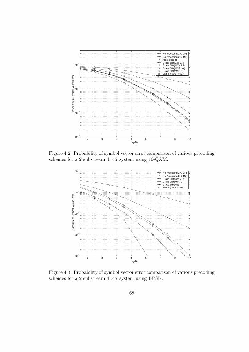
−2 0 2 4 6 8 10 1210

−3

10−2

10−1

100

Eb/N

0

Pro

babi

lity

of S

ymbo

l Vec

tor

Err

or

No Precoding(2×2 ZF)No Precoding(2×2 ML)Ant Select(ZF)Grass 6Bit(Cap ZF)Grass 6Bit(MSV ZF)Grass 6Bit(MSE det)Grass 6Bit(MSE tr)MMSE(Sum Power)

Figure 4.2: Probability of symbol vector error comparison of various precodingschemes for a 2 substream 4× 2 system using 16-QAM.

−2 0 2 4 6 8 10 1210

−4

10−3

10−2

10−1

100

Eb/N

0

Pro

babi

lity

of S

ymbo

l Vec

tor

Err

or

No Precoding(2×2 ZF)No Precoding(2×2 ML)Grass 6Bit(Cap ZF)Grass 6Bit(MSV ZF)Grass 6Bit(ML)MMSE(Sum Power)

Figure 4.3: Probability of symbol vector error comparison of various precodingschemes for a 2 substream 4× 2 system using BPSK.

68

−2 0 2 4 6 8 10 1210

−3

10−2

10−1

100

Eb/N

0

Pro

babi

lity

of S

ymbo

l Vec

tor

Err

or

No Precoding(4×4 ZF)No Precoding(4×4 ML)Ant Select(ZF)Grass 4Bit(MSV ZF)Grass 4Bit(MSE tr)MMSE(Sum Power)

Figure 4.4: Probability of symbol vector error comparison of various precodingschemes for a 4 substream 5× 4 system using 4-QAM.

Experiment 3: This simulation shows performance comparisons of pre-

coding schemes using 4-QAM modulation and four substreams. The results

are shown in Fig. 4.4. In this case, we simulated the probability of sym-

bol vector error curves for a 5× 4 limited feedback precoding with four bits of

feedback using SC-MSV and SC-MSE. This simulation shows the performance

differences between the different precoder selection criteria. Precoding using

SC-MSV yields approximately a 0.4dB improvement over antenna selection.

Using limited feedback precoding with SC-MSE and the trace cost function

within 1.1dB of unquantized MMSE precoding with the sum power constraint.

Experiment 4: We simulated three substream precoding on a 6 × 3

wireless system in this experiment using 16-QAM with results shown in Fig.

4.5. We used limited feedback precoding with six bits of feedback. Limited

69

−3 −2 −1 0 1 2 3 4 5 6 7 810

−2

10−1

100

Eb/N

0

Pro

babi

lity

of S

ymbo

l Vec

tor

Err

or

No Precoding(3×3 ZF)No Precoding(3×3 ML)Ant Select(ZF)Grass 6Bit(Cap ZF)Grass 6Bit(MSV ZF)Grass 6Bit(MSE tr)MMSE(Sum Power)Optimal(ZF)

Figure 4.5: Probability of symbol vector error comparison of various precodingschemes for a 3 substream 6× 3 system using 16-QAM.

feedback precoding with SC-Capacity performed approximately the 0.25dB

better than antenna selection. Limited feedback precoding using SC-MSV

and SC-MSE with the trace cost function both performed approximately the

same. They both provide around a 0.25dB improvement over SC-Capacity

and perform within 1dB of unquantized optimal precoding using ZF decoding.

Note that all selection criteria outperformed unprecoded spatial multiplexing

using an ML receiver. This shows though the power of precoding: near ML or

better than ML performance with low complexity receivers at the expense of

feedback.

Experiment 5: This experiment simulated three substream precoding

on a 6× 3 wireless system in this experiment using BPSK. This experiment’s

results are presented in Fig. 4.6. Once again, six bit limited feedback precod-

70

−2 0 2 4 6 8 1010

−4

10−3

10−2

10−1

100

Eb/N

0

Pro

babi

lity

of S

ymbo

l Vec

tor

Err

or

No Precoding(3×3 ZF)No Precoding(3×3 ML)Grass 6Bit(MSE det)Grass 6Bit(ML)MMSE(Sum Power)MMSE(Max SV)

Figure 4.6: Probability of symbol vector error comparison of various precodingschemes for a 3 substream 6× 3 system using BPSK.

ing was used. Precoding using SC-MSE with the determinant cost function

provides approximately a 0.4 dB array gain compared to unprecoded spatial

multiplexing using ML decoding. Unquantized MMSE precoding with the

maximum singular value constraint performs only 0.8dB better than the six

bit limited feedback precoder. Using quantized precoding with ZF decoding

provides approximately a 1dB gain over quantized precoding using SC-MSE

with the determinant cost function at a probability of symbol vector error

of 10−3. Quantized precoding using ML decoding and SC-ML outperforms

unquantized MMSE precoding with the sum power constraint by more than

1.8dB.

Experiment 6: The purpose of this experiment is to demonstrate the

problems associated with directly quantizing the matrix channel H. The re-

71

−2 0 2 4 6 8 10 12 14 16 1810

−3

10−2

10−1

100

Eb/N

0

Vec

tor

SE

R

MMSE(Max SV)Quant. Chann. MMSE(16 bit)Grass 6bit(MSE det)

Figure 4.7: Probability of symbol vector error comparison for direct chan-nel quantization, unquantized MMSE, and limited feedback precoding on a 2substream 4× 2 system using 16-QAM.

sults are presented in Fig. 4.7. This experiment considered a 4 × 2 wireless

system using two substrems and 16-QAM. Directly quantizing the channel

with sixteen bits of feedback performs approximately 4.7dB worse than a six

bit limited feedback precoder at a probability of symbol vector error of 10−2.

The limited feedback precoder obtains performance approximately identical

to that of the unquantized MMSE precoder with the maximum singular value

power constraint.

72

Chapter 5

Multi-Mode Precoding

This chapter overviews a new adaptive modulation for MIMO systems called

multi-mode precoding. Section 5.1 introduces the multi-mode precoded spatial

multiplexing system model. Criteria for choosing the optimal matrix from the

codebook is presented in Section 5.2. We discuss the implementation of multi-

mode precoding in systems with perfect CSI at the transmitter in Section 5.3.

The case of no CSI at the transmitter is considered in Section 5.4. Section

5.5 characterizes the diversity and multiplexing gains of multi-mode precod-

ing. The relationship between limited feedback multi-mode precoding and

covariance quantization is explored in Section 5.6. Section 5.7 illustrates the

performance improvements over previously proposed techniques using Monte

Carlo simulations of the symbol error rate and mutual information.

c© 2004 IEEE. Reprinted, with permission, from D. J. Love and R. W. Heath Jr.,“Multi-Mode Precoding Using Linear Receivers for MIMO Wireless Systems,” submitted toIEEE Transactions on Signal Processing.

73

5.1 System Overview

The Mt transmit and Mr receive antenna MIMO wireless system studied in

this chapter is shown in Fig. 5.1. For each channel use, R bits are demul-

tiplexed into M different bit streams. Each bit stream is modulated using

the same constellation S, producing a vector sk at the kth channel use. This

means that each substream carries R/M bits of information. The spatial mul-

tiplexing symbol vector sk = [sk,1 sk,2 . . . sk,M ]T is assumed to have power

constraints so that Esk[sks

∗k] = Es

MIM . Note that this means the average of the

total transmitted power at any channel use is independent of the number of

substreams M .

SpatialMultiplexer

Linearreceiver

+

+...

...H

v

v1,k

Mr,k

yksk

FM

M: # substreamsFM chosen from

codebook FM

...

FM sk

SymbolDetectorbits

G yk

sk

Figure 5.1: Block diagram of a limited feedback precoding MIMO system.

An Mt×M linear precoding matrix FM maps sk to an Mt-dimensional

spatio-temporal signal that is transmitted on Mt transmit antennas. The

transmitted signal vector encounters an Mr × Mt matrix channel H before

being added with an Mr-dimensional white Gaussian noise vector vk. Assum-

ing perfect pulse-shaping, sampling, and timing, this formulation yields an

input-output relationship

y = HFMs + v (5.1)

where the channel use index k has been suppressed because we are interested

in vector-by-vector detection of sk. We assume that H has i.i.d. entries with

74

each distributed according to CN (0, 1). We employ a block-fading model where

the channel is constant over multiple frames before independently taking a

new realization. As well, the noise vector v is assumed to have i.i.d. entries

distributed according to CN (0, N0).

The matrix HFM can be thought of as an effective channel. The re-

ceiver decodes y using this effective channel and a linear receiver. It is as-

sumed that the receiver has perfect knowledge of H and FM . The receiver

applies an M ×Mr matrix transformation G to y and then independently de-

tects each entry of Gy. If a zero-forcing (ZF) decoder is used, G = (HFM)†.

Minimum mean squared error (MMSE) decoding uses G = [F∗MH∗HFM +

(N0M/Es)IM ]−1F∗MH∗.

Note that the total instantaneous transmitted power for this system is

given by s∗F∗MFMs. The precoder matrix FM must therefore be constrained

in order to limit the transmitted power. We will restrict λ21{FM} ≤ 1 in

order to limit the peak-to-average ratio. This means that Es [s∗F∗MFMs] ≤Es regardless of the modulation scheme or the value of M. It was shown in

[28],[72],[73] that matrices of this form that optimize MSE, capacity, and total

channel power are all members of the set U(Mt, M) = {U ∈ CMt,M | U∗U =

IM}. For this reason, we will further restrict that FM ∈ U(Mt,M) for any

chosen value of M.

The key difference between multi-mode precoding and previously pro-

posed linear precoders is that M is adapted using current channel conditions

by allowing M to vary between 1 and Mt. We refer to the value of M as the

mode of the precoder. Usually, only a subset of the Mt possible modes can be

chosen. Examples of why only subsets of {1, . . . , Mt} might be chosen include

that i.) R/M is an integer for only a few of the modes between 1 and Mt

75

and ii.) system architecture only supports a subset. We will denote the set

of supported mode values as M. For example, if R = 8 bits and Mt = 4 then

only modes in the set M = {1, 2, 4} can be supported. Another example is a

dual-mode precoding where M = {1, Mt}.We assume that a selection function g : CMr×Mt →M picks the “best”

mode according to some criterion, and we set M = g(H). After M is chosen,

the precoder FM is chosen from a set FM ⊆ U(Mt,M) using a selection func-

tion fM : CMr×Mt → FM . Therefore, FM = fM(H). This means that there

are |M| different precoder selection functions. Note that we have made no

assumptions about the number of matrices in FM .

We consider two different transmitter CSI scenarios: full transmitter

CSI and zero transmitter CSI. These are the two extremes of transmitter

channel knowledge. The full transmitter CSI assumption is approximately

valid for a time division duplexing (TDD) system transmitting over a channel

that changes slowly in comparison to the duplexing period. The assumption of

zero channel knowledge approximates a frequency division duplexing (FDD)

system where the forward and reverse frequency bands are separated by a

frequency bandwidth much larger than the channel coherence bandwidth.

5.2 Multi-Mode Precoder Selection

The selection of the mode and precoder matrix will determine the performance

of the entire system. Because we are interested in constructing a high-rate

signaling scheme with low error rates, we will present bounds on the probability

of symbol vector error (i.e. the probability that the linear decoder returns at

least one symbol in error). As stated earlier, we consider receivers using ZF

76

and MMSE linear receivers. We will also review the capacity results for MIMO

systems both with and without transmitter CSI.

5.2.1 Performance Discussion

The selection criterion used to choose M and FM must tie directly to the

resulting performance of the precoded spatial multiplexing system. We will

address selection details based on two different performance measures: proba-

bility of error and capacity.

Probability of Error

It was shown in [71] that the effective SNR of the kth substream after linear

processing is given by

SNR(ZF )k (FM) =

Es

MN0[F∗MH∗HFM ]−1k,k

(5.2)

for ZF decoding and

SNR(MMSE)k (FM) =

Es

MN0[F∗MH∗HFM + (MN0/Es)IM ]−1k,k

− 1 (5.3)

for MMSE decoding where A−1k,k is entry (k, k) of A−1. The minimum substream

SNR, given by

SNRmin(FM) = min1≤k≤M

SNRk(FM), (5.4)

is an important parameter that will be used to characterize performance. For

ZF and MMSE decoding, SNRmin(FM) can be bounded by [71]

SNRmin(FM) ≥ λ2M{HFM} Es

MN0

. (5.5)

Therefore, the minimum singular value of the effective channel is often an

important parameter in linear precoded MIMO systems. Because the linear

77

precoding matrix FM is restricted to lie in the set U(Mt,M),

λM{HFM} ≤ λM{H} (5.6)

by the Poincare separation theorem [83], p. 190.

We are more interested, however, in tight bounds on the probability

of symbol vector error. Let dmin(M, R) denote the minimum distance for

the constellation S used when R/M bits are modulated per substream and

Ne(M, R) denote the average number of nearest neighbors of S. Given a matrix

channel H, the conditional probability of symbol vector error can be bounded

by the Nearest Neighbor Union Bound (NNUB) as [96]

Pe(H) ≤ 1−(

1−Ne(M,R)Q

(√SNRmin

d2min(M,R)

2

))M

. (5.7)

where SNRmin is computed for the given linear receiver. In stochastic chan-

nels, this average NNUB on the probability of symbol vector error is given by

taking the expectation of (5.7),

Pe = EH[Pe(H)]

≤ 1− EH

(1−Ne(M, R)Q

(√SNRmin

d2min(M, R)

2

))M . (5.8)

The NNUB is asymptotically tight [96], so the bound can be used to

determine the diversity order of a communication system. A MIMO wireless

system is said to have diversity order d [36] if

d = − limEs/N0→∞

log(Pe)

log(Es/N0). (5.9)

Diversity order, or diversity gain, is one of the fundamental parameters for

MIMO systems. The diversity order is always bounded above by the product

of the number of transmit and receive antennas, MtMr.

78

Capacity

The mutual information of the channel HFM assuming uncorrelated Gaussian

signaling on each antenna, denoted CUT , is well-known to be

CUT (FM) = log2 det

(IM +

Es

MN0

F∗MH∗HFM

). (5.10)

The notation CUT is used because this is commonly called the uninformed

transmitter (UT) capacity (i.e. no transmitter CSI) [16]. Note that this is

not really a “capacity” expression in the sense of distribution maximization

because we assume a fixed distribution [93]. We will, however, refer to (5.10)

as the capacity of the effective channel HFM when there is no form of CSI at

the transmitter in order to follow existing terminology in the MIMO literature.

When transmitter and receiver both have perfect knowledge of H and

FM the capacity is found by waterfilling [1], [16], [17]. Let r = rank(HFM).

The capacity of the informed transmitter is given by

CIT (FM) =r∑

j=1

log2

(1 +

Es

MN0

γjλ2j{HFM}

)(5.11)

where

∑rj=1 γj = M and γj = max

(0, µ− MN0

Esλ2j{HFM}

).

Just as diversity order is often used to characterize probability of error

performance, multiplexing gain can be used to characterize spectral efficiency.

Let R(ES/N0) denote the supported data rate as a function of SNR. A MIMO

wireless system is said to have a multiplexing gain of c [36] if

c = limEs/N0→∞

R(Es/N0)

log(Es/N0). (5.12)

Multiplexing gain is a fundamental property and, in our system, will be

bounded from above by min(Mt,Mr).

79

5.2.2 Selection Criteria

We will present probability of error and capacity selection. The probability

of error selection is based on the previous work in [40], [71], [97], [98] while the

capacity selection is similar to work presented in [65], [71], [99].

Probability of Error Selection

Assuming a probability of error selection criterion, the optimal selection cri-

terion would obviously be to choose the mode and precoder that provide the

lowest probability of symbol vector error. Selection using this criterion, how-

ever, is unrealistic because closed-form expressions for the probability of vector

symbol error conditioned on a channel realization are not available to the au-

thors’ knowledge. The NNUB can be successfully employed in place of this

bound for asymptotically tight selection. Using the NNUB result in Section

5.2.1, the following selection criterion is obtained.

NNUB Selection Criterion: Choose M and FM such that

g(UB)(H) = argminm∈M

(1−

(1−Ne(m,R)Q

(√SNRmin(f

(UB)m (H))

d2min(m,R)

2

))m)

(5.13)

f(UB)M (H) = argmin

F′∈FM

1−(

1−Ne(M, R)Q

(√SNRmin(F′)

d2min(M, R)

2

))M

.

(5.14)

The value of Ne(M, R) and dmin(M, R) can be computed offline and

stored in the receiver’s memory. The cost function can be implemented us-

ing a brute force search when there are only a finite number of matrices per

codebook. Unfortunately, the Q-function is often problematic to implement.

80

This issue can be overcome by further simplifying the cost function evaluated

in (5.14). The Q-function in (5.14) numerically dominates the constant terms

because it decreases exponentially. For this reason, it is often beneficial to use

the following approximate selection criterion.

SNR Selection Criterion: Choose M and FM such that

g(SNR)(H) = argmaxm∈M

SNRmin(f (SNR)m (H))d2

min(m,R)

f(SNR)M (H) = argmax

F′∈FM

SNRmin(F′). (5.15)

The SNR criterion represents a large complexity cost savings compared

to the NNUB criterion because of the removal of the Q-function. There are

two problems, however, with the SNR selection criterion. First, the functions

f(SNR)M (H) and g(SNR)(H) are coupled. This means that the functions can not

be implemented serially because f(SNR)m (H) must be computed for all m ∈M

before g(SNR)(H) is evaluated. The second problem is that the NNUB and SNR

selection criteria provide no intuition about the effect of a channel’s structure

on mode selection. Intuitively, the singular value structure of the channel

should have a natural mode of communication.

Note that HFM is at most a rank M matrix. Thus for each value of M

Es

MN0

maxF′∈FM

λ2Mt{HF′} ≤ max

F′∈FM

SNRmin(F′) ≤ Es

MN0

maxF′∈FM

λ2M{HF′} (5.16)

by the Poincare Separation Theorem [83], pp. 190. A selection criterion based

on selecting a mode only if the best achievable SNR approximately minimizes

the NNUB. This corresponds to the following selection criterion.

81

Singular Value (SV) Selection Criterion: Choose M and FM such that

g(SV )(H) = argmaxm∈M

λ2m{H}m

d2min(m,R) (5.17)

f(SV )M (H) = argmax

F′∈FM

λ2M{HF′}. (5.18)

Despite the fact that this bound is approximate, the probability of error

performance was shown in [40] to be quite close to both the SNR selection and

NNUB selection. The important advantage of this criterion is that the selection

of M and FM are decoupled. In particular, the computation of the smallest

singular value of HF′ for all codebook matrices in FM must only be completed

for one value of M rather than for every value in M. The criterion also gives a

clear picture of the relationship between a given channel realization and mode

selection. The channel rank and conditioning dictate the dimensionality of the

transmitted symbol vector.

Capacity Selection

While capacity selection is not optimal from a probability of error point-of-

view, it can provide insight into the attainable spectral efficiencies given the

multi-mode precoding system model. Because the uninformed transmitter

capacity is evaluated in closed-form given a matrix channel, the following

criterion can be succinctly stated.

Capacity Selection Criterion: Choose M and FM such that

g(Cap)(H) = argmaxm∈M

CUT (fm(H))

f(Cap)M (H) = argmax

F′∈FM

CUT (FM). (5.19)

82

5.2.3 Minimum Distance Calculations

The minimum distance expressions for dmin(M, R) often have closed-form ex-

pressions for common calculations. Consider the minimum distance of the

beamforming constellation (i.e. M = 1) dmin(1, R). The squared minimum

beamforming constellation distance for QAM constellations is given by

d2min(1, R) =

6Es

2R − 1

and for PSK constellations by

d2min(1, R) = 4Es sin2

( π

2R

).

When M > 1,

d2min(M, R) = d2

min(1, R/M).

The SNR and SV selection criteria both require the use of the ratios of

d2min(m1, R)/d2

min(m2, R) for m1,mr ∈M. This simplifies to

d2min(m1, R)

d2min(m2, R)

=2R/m2 − 1

2R/m1 − 1

for QAM constellations and

d2min(m1, R)

d2min(m2, R)

=sin2

(π

2R/m1

)

sin2(

π2R/m2

)

for PSK constellations.

Digital implementation of the cosine function is often challenging. For

high-rates, the small angle approximation can be used for PSK constellations

yielding

d2min(1, R) ≈ 4Es

( π

2R

)2

. (5.20)

83

The QAM distance ratios also have a simplified form for large R. For large R

and QAM constellations,

d2min(m1, R)

d2min(m2, R)

= 2R(1/m2−1/m1). (5.21)

5.3 Multi-Mode Precoding: Perfect Transmit-

ter Channel Knowledge

We will first address the application of multi-mode precoding when the trans-

mitter has perfect CSI. In this case, the transmitter knows H perfectly. An

example of this scenario is when the forwardlink channel matrix H can be

exactly estimated from the reverselink channel.

In this situation, the set Fm for each m ∈M will be defined as

Fm = U(Mt,m). (5.22)

The optimization of the different selection criteria is now over an uncountable

set. Thus the discrete search techniques employed in antenna selection are no

longer applicable. To our knowledge, the NNUB and SNR selection criteria are

not easily solved in the infinite feedback case. The SV and capacity selection

criteria, however, are easily solved.

Let H have singular value decomposition (SVD) given by

H = UΛV∗

where U ∈ U(Mr,Mr), V ∈ U(Mt, Mt), and Λ is a diagonal matrix with

λj{H} in position (j, j). Define

VM = V

IM

0

.

84

Note that the bound in (5.6) is achieved when

FM = VM . (5.23)

Because VM achieves the global upper bound over U(Mt,M), we can conclude

that for the SV selection criterion

f(SV )M (H) = VM . (5.24)

It was observed in [72],[73] that FM is a maximizer of CUT if and only if

it is a minimizer of the determinant of the mean squared error (MSE) matrix

considered in [28]. In [28], it was shown that VM minimizes the determinant

of the MSE matrix. Therefore, the capacity selection criterion matrix selection

function is defined as

f(Cap)M (H) = VM .

The form of the optimal precoding matrices illuminates an important

benefit of the proposed precoder. Multi-mode precoding is of practical in-

terest in TDD systems because it is actually reduced complexity waterfilling.

Instead of performing power pouring, only the precoder rank is adapted. This

complexity reduction is dramatic from both a power view and from a complex-

ity view. While waterfilling requires the matrix design techniques outlined in

Section 5.2.1, multi-mode precoding only requires knowledge of the M most

dominant singular vectors.

85

5.4 Limited Feedback Multi-Mode Precoding:

Zero Transmitter Channel Knowledge

We now consider the implementation of multi-mode precoding when the trans-

mitter has no form of channel knowledge. This design makes multi-mode

precoding practical even in systems that do not meet the assumption of full

transmitter CSI.

5.4.1 Codebook Model

The design of an adaptive modulator in a system without transmitter CSI is

daunting because we must find a simple method that allows the transmitter to

adapt to current channel conditions. We will overcome the lack of transmitter

CSI by using a low-rate feedback channel that can carry a limited number of

information bits, denoted by B, from the receiver to the transmitter.

Because the feedback channel can only support a limited number of

bits, the uncountable matrix sets employed in Section 5.3 are unusable. We

will therefore be required to take a different approach to the precoder de-

sign. In this limited feedback scenario, the precoder FM is chosen from a

finite set, or codebook, of NM different Mt × M precoder matrices FM =

{FM,1,FM,2, . . . ,FM,NM}. Thus, we assume that there is a codebook for each

supported mode value. Because there are a total of

Ntotal =∑

m∈MNm

codeword matrices, a total feedback of

B = dlog2(Ntotal)e =

⌈log2

( ∑m∈M

Nm

)⌉

86

bits is required for feedback. Feedback can thus be kept to a reasonable amount

by varying the size of NM for each mode.

There are two main problems associated with this codebook-based lim-

ited feedback system. First, we must determine how to distribute the Ntotal

codewords among the modes in M. The second problem is how to design FM

given M and NM . We present solutions for both of these problems in Sections

5.4.2 and 5.4.3.

5.4.2 Codeword Distribution

The feedback amount B is often specified offline by general system design

constraints. For example, only B bits of control overhead might be available

in the reverselink frames. For this reason, we will assume that B is a fixed

system parameter. Thus, we wish to understand how to distribute Ntot = 2B

codeword matrices among the |M| modes.

The first step in assigning codewords is the determination of a distor-

tion function. The distortion function must be specific to the selection function

used in order to maximize performance. We will design the distortion func-

tion by attempting to force the quantized multi-mode precoder to perform

identically to the unquantized (or perfect CSI) multi-mode precoder.

Because the NNUB, SNR, and SV selection all relate directly or indi-

rectly to maximizing λ2M{HFM}, we will define the distortion conditioned on

H and M to be

D(Pe)(FM ,M) =∣∣λ2

M{HVM} − λ2M{HFM}

∣∣2 =∣∣λ2

M{H} − λ2M{HFM}

∣∣2 .

87

The capacity selection will use the conditional distortion function given by

D(Cap)(FM ,M) =

∣∣∣∣log2 det

(IM +

Es

MN0

V∗MH∗HVM

)

− log2 det

(IM +

Es

MN0

F∗MH∗HFM

)∣∣∣∣2

. (5.25)

A key difference between two distortions is that the probability of error

distortion is independent of the SNR while the capacity distortion is dependent

on the SNR. This means that the capacity codebook would have to be modified

each time the SNR changes. This same SNR dependence also exists in the

capacity codebooks designed in [100].

Let M = {m1,m2, ..., m|M|}. We wish to minimize the average distor-

tion

D(Fm1 , . . . ,Fm|M|

)= EM [EH [D(fM(H), M) | M ]] (5.26)

using the appropriate distortion. We will approximate EH [D(fM(H),M) | M ]

using a uniform, high-resolution approximation [82], p. 163. This assumption

yields

EH [D(fM(H), M) | M ] ≈ K

N2M

(5.27)

where K is a positive real constant that depends on the chosen selection func-

tion but is constant for all mode numbers. Without this assumption the prob-

lem is virtually unsolvable because i.) the effective channel will no longer be

a Gaussian matrix and ii.) the distortion depends directly on the codebook.

This assumption also allows the codeword matrices to be allocated for the

different selection functions using the same optimization methods. Thus, the

optimization will not directly deal with D(Pe)(·, ·) or D(Cap)(·, ·). While this

approximation is very rough, it is sufficient enough for us to approximately

allocate the codewords among the |M| supported levels.

88

Plugging (5.27) into (5.26),

D(Fm1 , . . . ,Fm|M|

)≈ EM

[K

N2M

]=

∑m∈M

pmK

N2m

(5.28)

with pm = Prob(M = m) meaning the probability that the mode random

variable chooses m streams. Specifically, pm = Prob(g(SV )(H) = m

)for prob-

ability of error selection and pm = Prob(g(Cap)(H) = m

)for capacity selection.

We will minimize (5.28) given that

∑m∈M

Nm = Ntot (5.29)

and 0 < Nm < Ntot for all m ∈ M. Let N =[Nm1 Nm2 · · · Nm|M|−1

]T

. We

rewrite (5.28) using the function

Dapprox(N) =

|M|−1∑

l=1

pml

K

N2ml

+ pm|M|K(

Ntot −∑|M|−1

k=1 Nmk

)2 .

Thus we will solve for the matrix allocation values Nm1 , Nm2 , . . . , Nm|M|−1that

minimize Dapprox and then set

Nm|M| = Ntot −|M|−1∑

l=1

Nml.

Because the Hessian of Dapprox is a positive and diagonally dominant,

and thus positive-definite, matrix if 0 < Nm < Ntot for all m ∈ M, the

function Dapprox is convex. Thus the minimizer of Dapprox can be found by

solving for N that sets the gradient of Dapprox equal to zero. Evaluating the

partial derivative of Dapprox with respect to Nm for m ∈M gives

∂Dapprox

∂Nm

(N) = −pm2K

N3m

+ pm|M|2K(

Ntot −∑|M|−1

k=1 Nmk

)3 . (5.30)

89

The partial derivative ∂Dapprox

∂Nm(N) will be equal to zero when

3√

pm

Ntot −

|M|−1∑

k=1

Nmk

− 3

√pm|M|Nm = 0.

Solving the set of |M| − 1 linear equations to find the values of N that sets

the gradient equal to zero corresponds to the solution

N = NtotΦ−1p (5.31)

where

Φ = 3√

pm|M| I|M|−1 +

3√

pm13√

pm1 · · · 3√

pm1

3√

pm23√

pm2 · · · 3√

pm2

.... . .

...

3√

pm|M|−1· · · 3

√pm|M|−1

3√

pm|M|−1

and

p =[

3√

pm13√

pm2 · · · 3√

pm|M|−1

]T

. (5.32)

Eq. (5.31) will return values of Nm that are real numbers rather than

integers. This point can be corrected by simply rounding the numbers and

reenforcing (5.29). Care must also be taken when Mt ∈M. The codebook FMt

corresponds to choosing traditional spatial multiplexing. Thus IMt ∈ FMt . The

identity matrix, however, is the only matrix in FMt . The reason for this is that

if there existed F ∈ FMt with F 6= IMt then the performance of precoded spatial

multiplexing using F over uncorrelated Rayleigh fading would exactly match the

performance of traditional spatial multiplexing. This follows easily from the

fact that HF has the same distribution as H when H is an uncorrelated,

Rayleigh fading matrix [85]. Therefore either FMt = {IMt} or FMt is empty.

Thus when (5.31) gives NMt > 1, (5.31) can be used to recompute Nm for all

90

m ∈ M = M\{Mt}. This requires replacing the pm probabilities in (5.31)

with pm|M, the probability of mode m ∈ M given that the chosen mode is in

M and the constraint∑

m∈MNm = Ntot − 1 (5.33)

is satisfied.

5.4.3 Codebook Criterion Given the Number of Sub-

streams

Now that we have determined an algorithm that gives an approximate alloca-

tion of the possible codebook matrices among the modes, it is now imperative

to present the design of FM for each mode. There are two special cases of

the multi-mode precoder codebooks. The column vectors in F1 correspond to

beamforming vectors [59]. The design of limited feedback beamforming was

explored in [22], [52], [53], [59], [63]. In particular, it was shown in [59], [63] that

the set of vectors should be designed by thinking of the vectors as represent-

ing lines in CMt . The lines can then be optimally spaced by maximizing the

minimum angular separation between any two lines. The set FMt is trivially

designed because we will require that FMt = {IMt}. This precoder matrix

corresponds to sending a standard spatial multiplexing vector.

Codebook design for limited feedback precoding assuming a fixed num-

ber of substreams was studied in [72], [73], [101], [102] for a variety of se-

lection functions. The NNUB and SNR selection criteria both depend on

SNRmin(FM). As stated earlier, the minimum SNR can be approximately

maximized by maximizing λM{HFM}. It was shown in [102] that FM should

be designed by maximizing the minimum projection two-norm subspace dis-

91

tance between any two matrices in FM given by

dproj(FM,1,FM,2) = ‖FM,1F∗M,1 − FM,2F

∗M,2‖2. (5.34)

The capacity selection criterion, however, motivates the use of the Fubini-

Study subspace distance. Thus for the capacity selection criterion we would

try to maximize the minimum pairwise distance given by

dFS(FM,1,FM,2) = arccos∣∣det

(F∗M,1FM,2

)∣∣ . (5.35)

These codebooks can be easily designed using the matrix codebooks de-

signed for non-coherent constellations in [92]. The only modification needed is

to change the distance function to the projection two-norm subspace distance.

For more information on these designs consult [102].

5.5 Diversity Order & Multiplexing Gain

MIMO wireless systems have fundamental limits on the maximum attainable

diversity order and multiplexing gain. Both parameters are fundamental in

MIMO systems [36]. We will derive conditions for multi-mode precoding to

have maximum diversity order and multiplexing gain.

The following theorem addresses the conditions sufficient to obtain full

diversity order.

Theorem 2 If 1 ∈ M and N1 ≥ Mt then multi-mode precoding provides full

diversity order when using the NNUB selection criterion.

Proof It is shown in [38], that a limited feedback beamformer with a vector

codebook that spans CMt obtains full diversity order. It was shown in [59] that

92

this condition is satisfied when N1 ≥ Mt and the codebook design techniques

outlined in Section 5.4.3 are used. Because the NNUB presents an upper-

bound on the probability of error, a selection function based on this result will

only decrease the probability of error asymptotically when compared with a

beamforming-only system.

The achievability of full diversity order is a substantial benefit. Spatial

multiplexing has limited diversity order performance (ex. achieves diversity

order Mr for overly complex maximum likelihood decoding), so a large diversity

increase such as this adds considerable error rate improvements.

The next theorem addresses multiplexing gain.

Theorem 3 If Mt ∈M and NMt > 0 then multi-mode precoding provides full

multiplexing gain.

Proof It is shown in [36] that spatial multiplexing (i.e. using mode M = Mt)

provides full multiplexing gain. Because the transmission rate is independent

of the mode chosen, the rate growth will be proportional to min(Mt,Mr).

5.6 Relation to Covariance Quantization

The capacity analysis for MIMO systems with transmitter CSI relies on opti-

mizing the transmit covariance matrix. A MIMO system has a general input-

output relationship

y = Hx + v

with H and v defined as in (5.1). The capacity maximizes the covariance

matrix

Q = Ex [xx∗] . (5.36)

93

Covariance quantization, proposed in [100], [103], chooses Q from a

codebookQ = {Q1,Q2, . . . ,QN}. Assuming that s in (5.1) consists of indepen-

dent entries distributed according to CN (0, Es/M), the covariance matrix will

be (Es/M)FMF∗M . Thus multi-mode precoding quantizes the set of covariance

matrices assuming a rank constraint. Let

QM = {(Es/M)FF∗ | ∀ F ∈ FM}.

This allows multi-mode precoding to be reformulated as covariance quantiza-

tion with a codebook

Q =⋃

m∈MQm.

Multi-mode precoding is a rank constrained covariance quantization.

While the codebook matrices in [100] attempt to quantize a waterfilling so-

lution, chooses a covariance rank and then allocates equal power among each

mode. This avoids the power allocation problems associated with waterfilling.

5.7 Simulations

Limited feedback multi-mode precoding was simulated to exhibit the available

decrease in probability of error and the increase in capacity. The capacity

results are compared with the results in [100].

Experiment 1: This experiment addresses the probability of symbol

vector error of 4× 4 dual-mode precoding with a ZF receiver. The results are

shown in Fig. 5.2. The rate is fixed at R = 8 bits per channel use with QAM

constellations. Because the system is dual-mode, the set of supported modes

is M = {1, 4}. Four bits of feedback is assumed to be available. Limited

feedback beamforming using four bits (see [59], [63]) and spatial multiplexing

94

are simulated for comparison. Multi-mode precoding with the SV selection

criterion provides approximately a 0.25 dB performance improvement over

limited feedback beamforming. The SNR and NNUB selection criteria perform

approximately the same, 0.55 dB better than the SV selection criterion. These

gains are modest because of the restriction to dual-mode precoding.

−2 0 2 4 6 8 10 12

10−3

10−2

10−1

100

Eb/N

0

Pro

b. o

f Sym

bol V

ecto

r E

rror

Spatial MultiplexingBeamformingMM Precode (SV)MM Precode (SNR)MM Precode (NNUB)

Figure 5.2: Probability of symbol vector error performance for limited feedbackdual-mode precoding, limited feedback beamforming, and spatial multiplexing.

Experiment 2: In contrast to the first experiment, this experiment con-

siders a 4 × 4 MIMO system transmitting R = 8 bits per channel use with

M = {1, 2, 4}. Codebooks were designed using B = 5 bits of feedback. Con-

stellations were restricted to be QAM. Fig. 5.3 presents the simulation results.

Spatial multiplexing, unquantized beamforming (i.e. perfect CSI at the trans-

mitter), and unquantized MMSE precoding are shown for comparison. The

95

MMSE precoding was implemented as in [28] with the sum power constraint

and the trace cost function. Note that all of the selection criteria provide ap-

proximately the same probability of symbol vector error performance. Five bit

multi-mode precoding provides approximately a 5dB gain over full CSI beam-

forming. There is more than a 8.5dB gain over spatial multiplexing at an

error rate of 10−1. Interestingly, MMSE precoding with full transmit channel

knowledge, a less restrictive power constraint, and a superior receiver provides

only a 1.2dB gain over limited feedback multi-mode precoding.

−2 0 2 4 6 8 10 12 14 1610

−3

10−2

10−1

100

Eb/N

0

Pro

b. o

f Sym

bol V

ecto

r E

rror

Spatial MultiplexingBeamforming (Perfect CSI)MM Precode (SV)MM Precode (SNR)MM Precode (NNUB)MMSE (Perfect CSI)

Figure 5.3: Probability of symbol vector error performance for limited feedbackmulti-mode precoding, beamforming, and spatial multiplexing.

Experiment 3: The third experiment compares limited feedback and

perfect CSI multi-mode precoding. Again, we considered a 4×4 MIMO system

transmitting R = 8 bits per channel use. We used a zero-forcing receiver, QAM

96

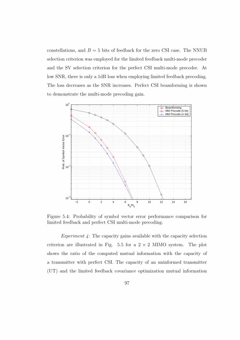
constellations, and B = 5 bits of feedback for the zero CSI case. The NNUB

selection criterion was employed for the limited feedback multi-mode precoder

and the SV selection criterion for the perfect CSI multi-mode precoder. At

low SNR, there is only a 1dB loss when employing limited feedback precoding.

The loss decreases as the SNR increases. Perfect CSI beamforming is shown

to demonstrate the multi-mode precoding gain.

−2 0 2 4 6 8 10 12 14 1610

−3

10−2

10−1

100

Eb/N

0

Pro

b. o

f Sym

bol V

ecto

r E

rror

BeamformingMM Precode (5 bit)MM Precode (∞ bit)

Figure 5.4: Probability of symbol vector error performance comparison forlimited feedback and perfect CSI multi-mode precoding.

Experiment 4: The capacity gains available with the capacity selection

criterion are illustrated in Fig. 5.5 for a 2 × 2 MIMO system. The plot

shows the ratio of the computed mutual information with the capacity of

a transmitter with perfect CSI. The capacity of an uninformed transmitter

(UT) and the limited feedback covariance optimization mutual information

97

results published in [100] are shown for comparison. Note that limited feedback

precoding outperforms limited feedback covariance optimization for both two

and three bits of feedback. This result is striking because, unlike covariance

optimization, multi-mode precoding does not require any form of waterfilling.

Thus our scheme, on average, always transmits with the same power on each

symbol substream. The high-rate feedback performance difference between

limited feedback covariance optimization and multi-mode precoding can be

most likely attributed to this power-pouring.

−10 −5 0 5 10 15 200.6

0.65

0.7

0.75

0.8

0.85

0.9

0.95

1

Es/N

0

Nor

mal

ized

Cap

acity

UTMM Precode (2bit)MM Precode (3bit)MM Precode (4bit)Blum (2bit)Blum (3bit)Blum (4bit)

Figure 5.5: Capacity comparison of multi-mode precoding, limited feedbackcovariance optimization [100], and the uninformed transmitter.

Experiment 5: The fifth experiment, shown in Fig. 5.6, compares the

simulated mutual information for multi-mode precoding with the capacity of

the UT and beamforming (i.e. unit rank covariance constraint). We assumed

98

perfect transmitter CSI for the multi-mode precoding and a supported mode

set M = {1, 2, 3, 4}. The mutual informations were normalized at each SNR

value by the capacity of a MIMO system with perfect channel state infor-

mation. Multi-mode precoding provides dramatic gains over other the other

systems by always obtaining greater than 97.5% of the total system capacity.

Thus the equal power assumption and rank tradeoff provide a close approx-

imation to optimal waterfilling. This is an amazing achievement considering

that rank adaptation is only rudimentary waterfilling.

−10 −5 0 5 10 15 200.4

0.5

0.6

0.7

0.8

0.9

1

1.1

Es/N

0

Nor

mal

ized

Cap

acity

UTBeamforming (Perfect CSI)MM Precode (∞bit)

Figure 5.6: Capacity comparison of multi-mode precoding with an infiniteamount of feedback, beamforming, and an uninformed transmitter.

Experiment 6: The final experiment compares infinite resolution multi-

mode precoding, limited feedback multi-mode precoding, and the UT capacity

for a 3 × 3 MIMO system. The results are shown in Fig. 5.7. We considered

99

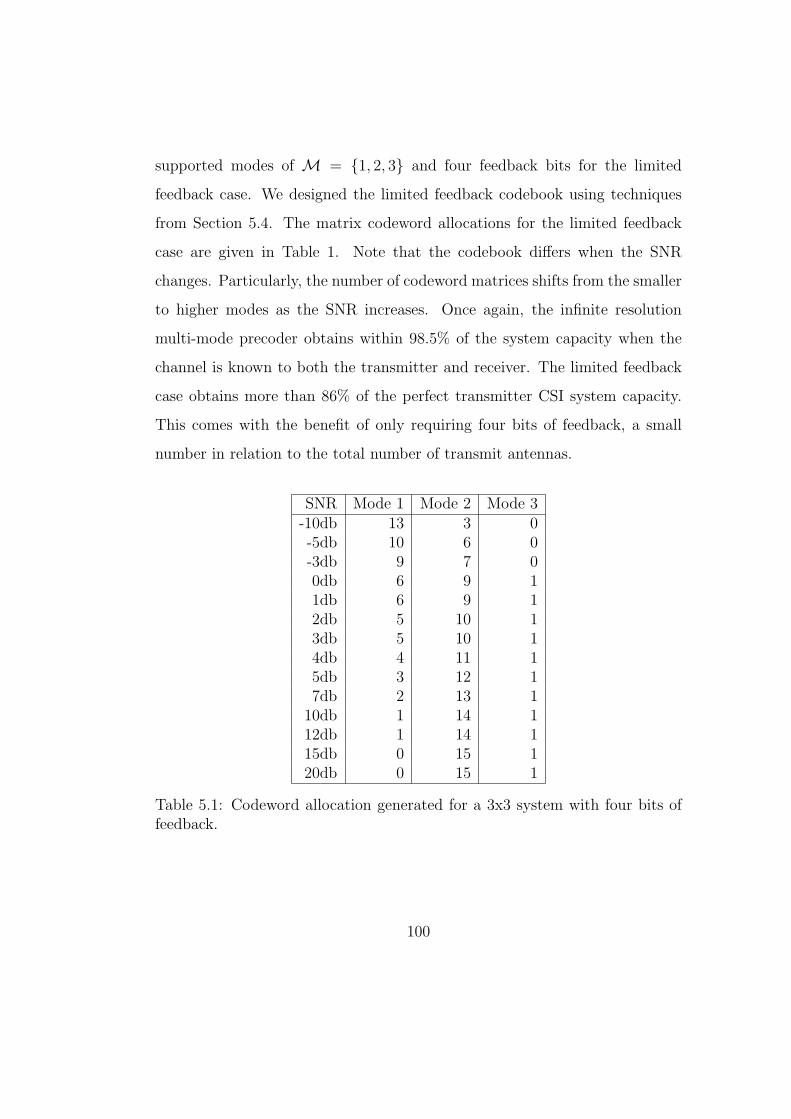
supported modes of M = {1, 2, 3} and four feedback bits for the limited

feedback case. We designed the limited feedback codebook using techniques

from Section 5.4. The matrix codeword allocations for the limited feedback

case are given in Table 1. Note that the codebook differs when the SNR

changes. Particularly, the number of codeword matrices shifts from the smaller

to higher modes as the SNR increases. Once again, the infinite resolution

multi-mode precoder obtains within 98.5% of the system capacity when the

channel is known to both the transmitter and receiver. The limited feedback

case obtains more than 86% of the perfect transmitter CSI system capacity.

This comes with the benefit of only requiring four bits of feedback, a small

number in relation to the total number of transmit antennas.

SNR Mode 1 Mode 2 Mode 3-10db 13 3 0-5db 10 6 0-3db 9 7 00db 6 9 11db 6 9 12db 5 10 13db 5 10 14db 4 11 15db 3 12 17db 2 13 1

10db 1 14 112db 1 14 115db 0 15 120db 0 15 1

Table 5.1: Codeword allocation generated for a 3x3 system with four bits offeedback.

100

−10 −5 0 5 10 15 200.5

0.6

0.7

0.8

0.9

1

1.1

Es/N

0

Nor

mal

ized

Cap

acity

UTMM Precode (4 bit)MM Precode (∞ bit)

Figure 5.7: Capacity comparison of multi-mode precoding with an infiniteamount of feedback, multi-mode precoding with four feedback bits, and anuninformed transmitter.

101

Chapter 6

Practical Aspects

The analysis presented in the preceding chapters made several assumptions

that would be questionable in real systems. This section will address four

of the major issues: spatial correlation, feedback delay, channel estimation

error, and feedback error. The use of limited feedback schemes in broadband

communications is also addressed.

6.1 Effect of Spatial Correlation

The effect of spatial correlation is often incorporated into the channel model.

While the matrix Rayleigh fading channel is commonly used for system design

[16], [17], several modifications have been proposed to the channel model to

more realistically simulate systems. We will consider these systems along with

measurement data.

In any wireless system, the “optimal” solution to test system perfor-

mance is to actually build the system. While this is impractical in nearly

every setting, simulations using actual channel measurements can provide a

102

flexible environment for making algorithmic tradeoffs. Prof. Murat Torlak at

The University of Texas at Dallas (UTD) has spearheaded the development of

an eight transmit antenna by one receive antenna testbed. The system uses a

carrier frequency of 2415 MHz and transmits a single tone at 10 dBm.

Figure 6.1: The UTD antenna array is an eight antenna circular array.

Experiment 1: Precoded OSTBCing was simulated on the channel data

collected by Torlak. The date was collected in a corridor of the Erik Jonsson

building with the antenna array transmitting from a lab approximately 50

feet away. The transmission was non-line-of-sight with the transmitter and re-

ceiver being separated by three walls. This experiment tested antenna subset

103

selection, six bit precoding, and an unprecoded two-antenna Alamouti code

on an 8× 1 system transmitting 16-QAM. The results are shown in Fig. 6.2.

The limited feedback precoding system still provides around a 1dB gain com-

pared to antenna subset selection. This clearly presents the benefits of limited

feedback in “real-world channels.”

−10 −8 −6 −4 −2 0 2 4 6 8 10

10−2

10−1

100

Es/N

0 (dB)

Pro

babi

lity

of S

ymbo

l Err

or

No Precoding(2×1)Antenna SubsetGrass 6Bit

Figure 6.2: Precoded OSTBC performance tested on UTD channel measure-ments.

The first MIMO channel models proposed by the measurement commu-

nity were ray based models. Ray based channel models are popular because

they mathematically simulate (in some sense) the effect of actual scatters.

The most well-known of the MIMO ray based models is the 3GPP/3GPP2

channel model. The 3GPP/3GPP2 MIMO channel model, overviewed in

[104], generates each entry of the channel matrix H as a function of the number

of specular wave components received K. The model uses numerous param-

104

eters in order to generate a realization. This model is primarily a function

of the angle of arrival (AoA) and angle of departure (AoD) of each of the

multipaths. The model allows for simulation in both line-of-sight (LOS) and

non-line-of-sight (NLOS).

The channel model can use three different simulation environments:

urban macrocell, suburban macrocell, and urban microcell. Further descrip-

tions of the assumptions for each of these simulation environments is included

in [104]. The channel is a function of 13 different parameters including AOA,

AOD, wave number, transmit antenna gain, receive antenna gain, mobile ve-

locity, mobile velocity vector angle, etc.

Despite the large number of variables, the channel is essentially a stan-

dard ray based channel model for transmit/receive uniform linear arrays (ULAs).

Let Dr (Dt) denote the receive (transmit) antenna spacing, θr (θt) denote the

AoA (AoD), and λ denote the carrier wavelength. A ray based channel is

simulated as [105]–[107]

H =K∑

l=1

αl · ar(θrl)∗at(θtl) (6.1)

where

ar(θr) =

[1 exp

(2π

λjDr sin(θr)

)· · · exp

(2π

λj(Mr − 1)Dr sin(θr)

)],

at(θt) =

[1 exp

(2π

λjDt sin(θt)

)· · · exp

(2π

λj(Mt − 1)Dt sin(θt)

)],

θrl(θtl) is the AoA (AoD) for the lth specular wave component, and αl is the

per wave gain.

Channel generation using (6.1) requires a distribution for θr and θt.

These two angles are usually generated independently using the same distri-

bution. Popular distributions include the Laplacian, Gaussian, and truncated

105

uniform. This model can also be generalized to fit into the stochastic local

area channel (SLAC) model discussed in [105] by changing the form of the

array response vectors. The SLAC model sums over all specular components

assuming known path delays, wavevectors, and receiver translation vectors.

The Cost 259 model is a popular MIMO ray-based channel model [108],

[109]. The model uses a fixed number of clusters and generates a certain

number of rays per cluster. Each cluster has a mean AoA and AoD associated

with it. Each ray has a different Rayleigh distributed path gain.

Experiment 2: This experiment simulated a 4×4 precoded spatial mul-

tiplexing system transmitting 4-QAM on a six cluster Cost 259 channel model.

Two substreams were transmitted. To model insufficient local scattering, the

number of rays per cluster was set to one. The results are shown in Fig. 6.3.

Note that a diversity difference is still evident between the precoded and un-

precoded systems. In particular, there is a gain of approximately 4dB at an

error rate of 10−2 when using precoding.

Since the introduction of MIMO, researchers in the areas of wireless

channel measurement and electromagnetics recognized the need to develop

new stochastic channel models that closely matched reality. This specifically

motivated the Information Society Technologies (IST) Multi-Element Trans-

mit and Receive Antennas (METRA) Project [110] funded by the European

Union and a consortium of governments and companies. The goal was to de-

sign a channel model for MIMO performance evaluation that would match

measurements. In particular, their model generalizes the ray based models for

moderate to large numbers of scatterers. Practically, this number has been

found to be approximately K > 10 [106].

106

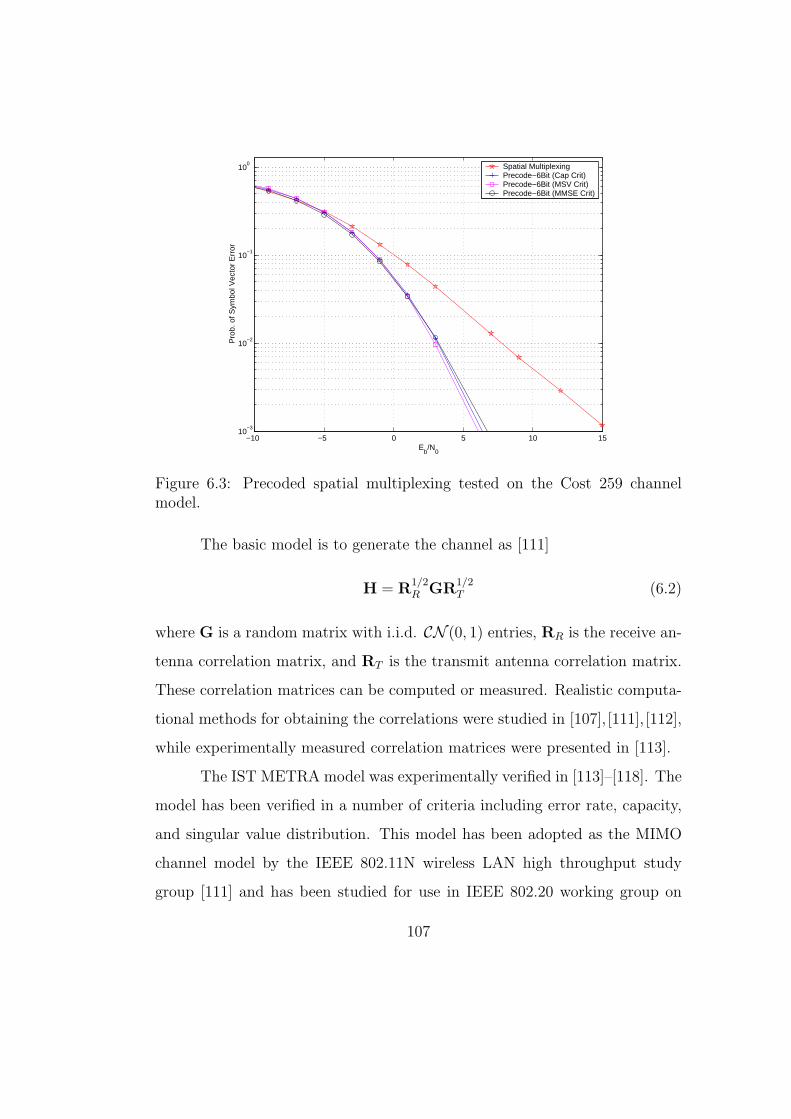
−10 −5 0 5 10 1510

−3

10−2

10−1

100

Eb/N

0

Pro

b. o

f Sym

bol V

ecto

r E

rror

Spatial MultiplexingPrecode−6Bit (Cap Crit)Precode−6Bit (MSV Crit)Precode−6Bit (MMSE Crit)

Figure 6.3: Precoded spatial multiplexing tested on the Cost 259 channelmodel.

The basic model is to generate the channel as [111]

H = R1/2R GR

1/2T (6.2)

where G is a random matrix with i.i.d. CN (0, 1) entries, RR is the receive an-

tenna correlation matrix, and RT is the transmit antenna correlation matrix.

These correlation matrices can be computed or measured. Realistic computa-

tional methods for obtaining the correlations were studied in [107], [111], [112],

while experimentally measured correlation matrices were presented in [113].

The IST METRA model was experimentally verified in [113]–[118]. The

model has been verified in a number of criteria including error rate, capacity,

and singular value distribution. This model has been adopted as the MIMO

channel model by the IEEE 802.11N wireless LAN high throughput study

group [111] and has been studied for use in IEEE 802.20 working group on

107

mobile broadband wireless access [119]. The model is thus expected to be the

cornerstone by which all future MIMO algorithms are tested before implemen-

tation.

Unlike ray based models, analytical error rate results can be derived

for the IST METRA model. Specifically, it is of interest to understand the

requirements that RR and RT must maintain to guarantee full diversity order.

We will first characterize the conditions needed for a beamformer to achieve

full diversity order.

Theorem 4 A wireless system employing limited feedback beamforming and

combining over memoryless, correlated Rayleigh fading channels provides full

diversity order if and only if the vectors in the beamforming feasible set span

CMt , the vectors in the combining feasible set span CMr , and the matrices RT

and RR are invertible.

Proof We will first prove the sufficiency of the conditions. Suppose that

the beamforming and combining vectors span CMt and CMr , respectively.

Note that the diversity order will always be less than or equal to MtMr be-

cause there are only MtMr independently fading parameters. Let W denote

the beamforming feasible set and Z denote the combining feasible set. We

can construct an invertible matrix B = R1/2T W = R

1/2T [w1 w2 · · · wMt ]

where wi ∈ W for all i. We can similarly construct an invertible matrix

C = R1/2R

∗Z = R

1/2R

∗[z1 z2 · · · zMr ] where zi ∈ Z for all i. Since the matrices

c© 2004 IEEE. Theorem reprinted, with permission, from D. J. Love and R. W. HeathJr., “Necessary and Sufficient Conditions for Full Diversity Order in Correlated RayleighFading Beamforming and Combining Systems,” accepted to IEEE Transactions on WirelessCommunications.

108

are invertible, we can define a singular value decomposition of each matrix

B = VLΛV∗R and C = ULΦU∗

R (6.3)

where VL and VR are Mt×Mt unitary matrices, Λ is a diagonal matrix with

diagonal entries λ1 ≥ λ2 ≥ . . . ≥ λMt > 0, UL and UR are Mr ×Mr unitary

matrices, and Φ is a diagonal matrix with diagonal entries φ1 ≥ φ2 ≥ . . . ≥φMr > 0.

For this system,

Γr = maxw∈W

maxz∈Z

|z∗Hw|2

≥ max1≤p≤Mr

max1≤q≤Mt

∣∣z∗pHwq

∣∣2

= max1≤p≤Mr

max1≤q≤Mt

∣∣∣(UR)∗p ΦU∗LGVLΛ (VR)q

∣∣∣2

d= max

1≤p≤Mr

max1≤q≤Mt

∣∣∣(U∗RΦGΛVR)(p,q)

∣∣∣2

(6.4)

≥ 1

MtMr

‖ΦGΛ‖22

≥ 1

MtMr

φ2Mr

λ2Mt

max1≤p≤Mr

max1≤q≤Mt

|gp,q|2 (6.5)

where (A)p represents the pth column of a matrix A, (A)(p,q) is the (p, q) entry

of a matrix A, andd= denotes equivalence in distribution. Eq. (6.4) used

the invariance of complex normal matrices to unitary transformation [85], and

(6.5) follows from the matrix norm bounds described in [120].

Noting that the maximum over the entries |gp,q|2 is the effective channel

gain for SD systems, we thus have that

Ps(Error) ≤ EG

[Ps

(Error

∣∣∣∣1

MtMr

φ2Mr

λ2Mt

γrSD

)](6.6)

with

γrSD= max

1≤p≤Mr

max1≤q≤Mt

|gp,q|2 EN0

.

109

This is the probability of symbol error for an uncorrelated Rayleigh fading

SD system with array gain shift of 1MtMr

φ2Mr

λ2Mt

which provides a diversity of

order MtMr. We have thus proven that the system achieves a diversity order

of MtMr.

Now we prove necessity. Let the subspace spanned by the vectors in

W after multiplication by R1/2T , denoted by SW , be of dimension Mw and the

subspace spanned by the vectors in Z after multiplication by R1/2R

∗, denoted

by SZ , be of dimension Mz. Suppose that MwMz < MtMr. We can then find

an Mt ×Mw matrix V that spans SW and an Mr ×Mz matrix U that spans

SZ with V∗V = IMw and U∗U = IMz . For both matrices, we can construct

square unitary matrices V and U by concatenating Mt − Mw and Mr − Mz

orthonormal vectors to V and U respectively.

Therefore,

Γr = maxw∈W

maxz∈Z

|z∗Hw|2

≤ maxa:a∗a=1

maxd:d∗d=1

β |d∗U∗GVa|2

= maxa:a∗a=1

maxd:d∗d=1

β

∣∣∣∣∣∣

d

0

∗

U∗GV

a

0

∣∣∣∣∣∣

2

d= max

a:a∗a=1max

d:d∗d=1β

∣∣∣∣∣∣

d

0

∗

G

a

0

∣∣∣∣∣∣

2

= β∥∥G(1:Mz ,1:Mw)

∥∥2

2(6.7)

where β = ‖RT‖2 ‖RR‖2, 0 and 0 are zero vectors, and G(1:Mz ,1:Mw) represents

the matrix formed from the first Mz rows and Mw columns of G. The expres-

sion in (6.7) is the effective channel gain for an Mw ×Mz MRT/MRC system

110

with an array gain shift. Therefore,

Ps(Error) ≥ EG

[Ps

(Error

∣∣∣∣ ‖RT‖2 ‖RR‖2γrMRC

)](6.8)

with

γrMRC= ‖G(1:Mz ,1:Mw)‖2

2

EN0

.

Note that an Mw×Mz MRT/MRC system provides a diversity order of

MwMz. Thus, the bounded system provides a diversity order less than or equal

to MwMz and thus less than MtMr. Since this bound is true for arbitrary EN0

,

we can conclude that the system does not achieve full diversity.

Theorem 4 provides the intuition that the set of possible beamformers

must always form a basis for the vector space of possible dominant singular

value directions. The correlation matrix plays an important role in the per-

formance because it shapes the set of beamforming vectors. Interestingly a

similar result can be derived for precoded OSTBCs.

Theorem 5 A precoded OSTBCing system with full rank correlation matrices

obtains a diversity of order MtMr if and only if the matrix E = [F1 F2 · · · FN ]

is full rank.

Proof We will first prove the “if” part of the statement using the contrapos-

itive. Suppose that E is not full rank.

Note that

maxF′∈F

‖HF′‖2F ≤ M max

F′∈F‖HF′‖2

2 ≤ M‖HE‖22. (6.9)

c© 2004 IEEE. Theorem reprinted, with permission, from D. J. Love and R. W. HeathJr., “Diversity Performance of Precoded Orthogonal Space-Time Block Codes Using LimitedFeedback,” accepted to IEEE Communications Letters.

111

Let R1/2T E = ULΣU∗

R where UL ∈ U(Mt,Mt), Σ an Mt×NM diagonal matrix

with entry λi{R1/2T E} at entry (i, i), and UR ∈ U(NM, NM). Because of the

rank deficiency in E, Σ will be of the form Σ = [ΣT

0]T where Σ consists

of the first rank(E) rows of Σ and 0 is a zero matrix. Substitution of the

singular value decomposition of R1/2T E in to (6.9) gives

maxF′∈F

‖HF′‖2F ≤ M‖RR‖2‖GULΣU∗

R‖22

= M‖RR‖2‖GUL[ΣT

0]T‖22

= M‖RR‖2‖GUL Σ‖22

≤ M‖RR‖2‖R1/2T E‖2

2‖GUL‖2F (6.10)

where GUL is the first rank(E) columns of GUL and (6.10) follows from

using the submultiplicative property of a matrix norm and of noting that

‖Σ‖22 = ‖R1/2

T E‖22.

Note that the matrix GUL is equivalent in distribution to G [85].

Therefore, we have upper-bounded the effective channel gain by the effective

channel gain of an rank(E) ×Mr multi-antenna system experiencing matrix

Rayleigh fading. A transmit diversity system with the effective channel gain

given by this upper bound would obtain a diversity order of rank(E) ·Mr <

MtMr [16]. Therefore, we can conclude that if E is not full rank then the

precoded OSTBC does not obtain full diversity order.

Now we will prove the converse. Suppose E is full rank. Then

maxF′∈F

‖HF′‖2F ≥ max

1≤i≤NM‖Hei‖2

2 ≥1

Mr

‖HE‖21.

Once again let R1/2T E have a singular value decomposition of R

1/2T E = ULΣU∗

R.

112

By substitution,

maxF′∈F

‖HF′‖2F ≥

1

Mr

‖HE‖21

=1

Mr

‖R1/2R GR

1/2T E‖2

1

≥ 1

NMMr

‖R1/2R GULΣ‖2

1 (6.11)

≥ λ2Mt{R1/2

T E}NMMr

‖R1/2R GUL‖2

1

≥ λ2Mt{R1/2

T E}NMMrM2

t

‖R1/2R GUL‖2

F (6.12)

where (6.11) uses the fact that ‖AU‖21 ≥ 1

n‖A‖2

1 when A ∈ Cm×n and U ∈U(n, n) [59].

Therefore, we have lower-bounded the effective channel gain by the

effective channel gain of an Mt×Mr transmit diversity system. GUL is equiv-

alent in distribution to an uncorrelated matrix Rayleigh fading channel [85]. A

system with a effective channel gain given by (6.12) has MtMr diversity order.

We can conclude that the precoded OSTBC obtains full diversity order [16].

We also performed numerous Monte Carlo simulations to verify the sys-

tem performance. These simulations used covariance matrices taken from ac-

tual measurement data and experimentally validated in [113]. The correlation

matrices were assumed fixed during the simulation.

Experiment 3: This experiment dealt with the simulation of precoded

16-QAM Alamouti codes on a 4 × 4 system. The channel was modeled using

the “pico decorrelated” measurements METRA model from [113]. Fig. 6.4

shows the performance of six bit limited feedback precoding, antenna subset

selection, and a 2 × 4 Alamouti code. Note that limited feedback precoding

113

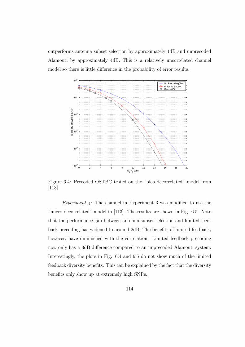
outperforms antenna subset selection by approximately 1dB and unprecoded

Alamouti by approximately 4dB. This is a relatively uncorrelated channel

model so there is little difference in the probability of error results.

0 2 4 6 8 10 12 14 16 18 2010

−5

10−4

10−3

10−2

10−1

100

Es/N

0 (dB)

Pro

babi

lity

of S

ymbo

l Err

or

No Precoding(2×4)Antenna SubsetGrass 6Bit

Figure 6.4: Precoded OSTBC tested on the “pico decorrelated” model from[113].

Experiment 4: The channel in Experiment 3 was modified to use the

“micro decorrelated” model in [113]. The results are shown in Fig. 6.5. Note

that the performance gap between antenna subset selection and limited feed-

back precoding has widened to around 2dB. The benefits of limited feedback,

however, have diminished with the correlation. Limited feedback precoding

now only has a 3dB difference compared to an unprecoded Alamouti system.

Interestingly, the plots in Fig. 6.4 and 6.5 do not show much of the limited

feedback diversity benefits. This can be explained by the fact that the diversity

benefits only show up at extremely high SNRs.

114

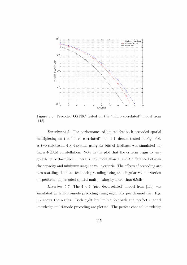
0 2 4 6 8 10 12 14 16 18 2010

−4

10−3

10−2

10−1

100

Es/N

0 (dB)

Pro

babi

lity

of S

ymbo

l Err

or

No Precoding(2×4)Antenna SubsetGrass 6Bit

Figure 6.5: Precoded OSTBC tested on the “micro correlated” model from[113].

Experiment 5: The performance of limited feedback precoded spatial

multiplexing on the “micro correlated” model is demonstrated in Fig. 6.6.

A two substream 4 × 4 system using six bits of feedback was simulated us-

ing a 4-QAM constellation. Note in the plot that the criteria begin to vary

greatly in performance. There is now more than a 3.5dB difference between

the capacity and minimum singular value criteria. The effects of precoding are

also startling. Limited feedback precoding using the singular value criterion

outperforms unprecoded spatial multiplexing by more than 6.5dB.

Experiment 6: The 4 × 4 “pico decorrelated” model from [113] was

simulated with multi-mode precoding using eight bits per channel use. Fig.

6.7 shows the results. Both eight bit limited feedback and perfect channel

knowledge multi-mode precoding are plotted. The perfect channel knowledge

115

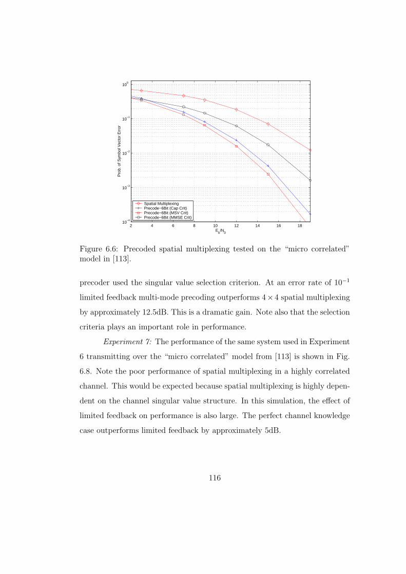
2 4 6 8 10 12 14 16 1810

−4

10−3

10−2

10−1

100

Eb/N

0

Pro

b. o

f Sym

bol V

ecto

r E

rror

Spatial MultiplexingPrecode−6Bit (Cap Crit)Precode−6Bit (MSV Crit)Precode−6Bit (MMSE Crit)

Figure 6.6: Precoded spatial multiplexing tested on the “micro correlated”model in [113].

precoder used the singular value selection criterion. At an error rate of 10−1

limited feedback multi-mode precoding outperforms 4×4 spatial multiplexing

by approximately 12.5dB. This is a dramatic gain. Note also that the selection

criteria plays an important role in performance.

Experiment 7: The performance of the same system used in Experiment

6 transmitting over the “micro correlated” model from [113] is shown in Fig.

6.8. Note the poor performance of spatial multiplexing in a highly correlated

channel. This would be expected because spatial multiplexing is highly depen-

dent on the channel singular value structure. In this simulation, the effect of

limited feedback on performance is also large. The perfect channel knowledge

case outperforms limited feedback by approximately 5dB.

116

−2 0 2 4 6 8 10 12 14 1610

−3

10−2

10−1

100

Eb/N

0

Pro

b. o

f Sym

bol V

ecto

r E

rror

Spatial MultiplexingMM Precode−8Bit (SV Crit)MM Precode−8Bit (PE Crit)MM Precode−∞Bit (SV Crit)

Figure 6.7: Multi-mode precoding tested on the “pico decorrelated” modelin [113].

6.2 Effect of Feedback Delay

In the previous chapters, it was assumed that there was no delay in the feed-

back channel. This assumption is quite erroneous in any real environment

where the receiver channel estimation period and low rate of the feedback

channel combine to produce an out-of-date precoder at the transmitter.

In order to quantify this performance loss, we simulated using the Clark-

Gans time correlation model from [76]. In this model, Gaussian random vari-

ables are multiplied in the frequency domain by a spectral mask before being

taken into the time domain via an inverse fast Fourier transform (IFFT). This

approach can be easily generalized to allow for different doppler spreads, sam-

pling periods, etc. We assumed that the system was using a carrier frequency

of 2400 MHz.

117

0 2 4 6 8 10 12 1410

−2

10−1

100

Eb/N

0

Pro

b. o

f Sym

bol V

ecto

r E

rror

Spatial MultiplexingMM Precode−8Bit (SV Crit)MM Precode−8Bit (PE Crit)MM Precode−∞Bit (SV Crit)

Figure 6.8: Multi-mode precoding tested on the “micro correlated” modelin [113].

Experiment 1: The first experiment tests the performance of limited

feedback precoded OSTBCs. A six bit precoded Alamouti code was tested

on a 4 × 2 MIMO system transmitting 16-QAM. It was assumed that the

environment had a maximum speed of 1m/s. Several different sampling rates

were simulated and are shown in Fig. 6.9. The limited feedback precoding

system still provides around a 1dB gain compared to antenna subset selection.

This clearly presents the benefits of limited feedback in “real-world channels.”

The plot shows that an update period of less than 0.1ms is required. Using an

update period of 0.2ms causes a 3.5dB performance loss.

Experiment 2: Six bit limited feedback precoded spatial multiplexing

was simulated at a speed of 0.5m/s on a 4 × 4 system transmitting 4-QAM.

The zero-delay case was simulated for comparison. The results are shown in

118

−5 0 5 10 15 20 2510

−4

10−3

10−2

10−1

100

Es/N

0 (dB)

Pro

babi

lity

of S

ymbo

l Err

or

No Precoding(2×1)Grass 6BitGrass 6Bit (0.1ms)Grass 6Bit (0.2ms)

Figure 6.9: Precoded OSTBC travelling at 1m/s with various sampling rates.

Fig. 6.10. At this reasonable indoor speed, the update period can be as high

as 10ms without causing any performance loss. Assuming a feedback channel

is present that can carry data at 1.5kb/s, we can support up to 15 bits of

feedback in this scenario.

Experiment 3: Fig. 6.11 shows the simulated performance of 4 × 4

multi-mode precoding with five feedback bits at a speed of 0.5m/s. It was

assumed that eight bits were transmitted at each channel use. The zero-delay

case was also simulated. Update periods of 6ms and 10ms are considered. At

these update periods, the performance loss only seems to show up at high

SNRs. This 10ms performance loss is approximately 0.5dB at an error rate of

10−3.

Experiment 4: The system in Experiment 2 was simulated assuming

a transmit SNR of 4dB. It was assumed that the mobile was traveling at

119

−8 −6 −4 −2 0 2 410

−3

10−2

10−1

100

Eb/N

0 (dB)

Pro

babi

lity

of S

ymbo

l Vec

tor

Err

or

Grass 6Bit (SV Criterion)Grass 6Bit (Cap Criterion)Grass 6Bit (MSE Criterion)Grass 6Bit delay 10ms (SV Criterion)Grass 6Bit delay 10ms (Cap Criterion)Grass 6Bit delay 10ms (MSE Criterion)

Figure 6.10: Precoded spatial multiplexing travelling at 0.5m/s with varioussampling rates.

1m/s. Fig. 6.12 presents the results. Note that all three criteria start to

perform worse than spatial multiplexing when the update period is larger

than the coherence time. Intuitively, this makes sense because the coherence

time of the channel is an approximate measure of the length of time before

channel realizations become independent. The plot also indicates that in most

scenarios an update period that is less than half the coherence time is needed.

6.3 Effect of Channel Estimation Error

An important consideration in MIMO wireless links is the estimation of the

matrix channel H. The limited feedback techniques developed in this disserta-

tion require that the receiver have knowledge of the current channel conditions.

120

−4 −2 0 2 4 6 8 10

10−3

10−2

10−1

100

Eb/N

0 (dB)

Pro

babi

lity

of S

ymbo

l Vec

tor

Err

or

MM PrecodeMM Precode delay 6msMM Precode delay 10ms

Figure 6.11: Multi-mode precoding travelling at 0.5m/s with various samplingrates.

This knowledge can be obtained by training, sending a signal known to both

the transmitter and receiver and using the known transmission to estimate the

channel.

For example, supposed the Mt×T matrix S was used for training. This

would yield an input-output relationship of

Y =

√ Es

Mt

HS + N (6.13)

where tr (S∗S) ≤ MtT and the entries of N are i.i.d. CN (0, N0). The ML

channel estimate would be given by [121]

HML =

√Mt

Es

YS∗ (SS∗)−1 , (6.14)

and the MMSE estimate is given by

HMMSE =

√Mt

Es

YS∗(SS∗ +

MtN0

Es

IMt

)−1

. (6.15)

121

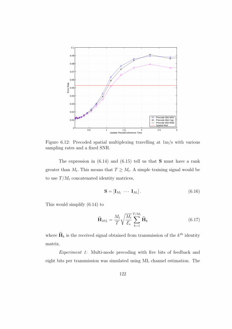
0.5 1 1.5 2 2.5 30

0.01

0.02

0.03

0.04

0.05

0.06

0.07

0.08

0.09

0.1

Update Period/Coherence Time

Err

or R

ate

Precode 6bit MSVPrecode 6bit CapPrecode 6bit MSESpatial Mult

Figure 6.12: Precoded spatial multiplexing travelling at 1m/s with varioussampling rates and a fixed SNR.

The expression in (6.14) and (6.15) tell us that S must have a rank

greater than Mt. This means that T ≥ Mt. A simple training signal would be

to use T/Mt concatenated identity matrices,

S = [IMt · · · IMt ] . (6.16)

This would simplify (6.14) to

HML =Mt

T

√Mt

Es

T/Mt∑

k=1

Hk (6.17)

where Hk is the received signal obtained from transmission of the kth identity

matrix.

Experiment 1: Multi-mode precoding with five bits of feedback and

eight bits per transmission was simulated using ML channel estimation. The

122

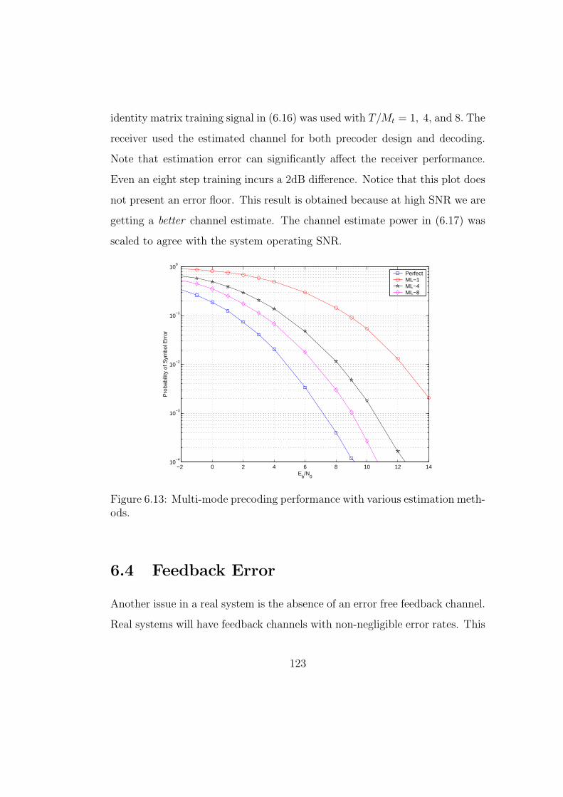
identity matrix training signal in (6.16) was used with T/Mt = 1, 4, and 8. The

receiver used the estimated channel for both precoder design and decoding.

Note that estimation error can significantly affect the receiver performance.

Even an eight step training incurs a 2dB difference. Notice that this plot does

not present an error floor. This result is obtained because at high SNR we are

getting a better channel estimate. The channel estimate power in (6.17) was

scaled to agree with the system operating SNR.

−2 0 2 4 6 8 10 12 1410

−4

10−3

10−2

10−1

100

Eb/N

0

Pro

babi

lity

of S

ymbo

l Err

or

PerfectML−1ML−4ML−8

Figure 6.13: Multi-mode precoding performance with various estimation meth-ods.

6.4 Feedback Error

Another issue in a real system is the absence of an error free feedback channel.

Real systems will have feedback channels with non-negligible error rates. This

123

follows because a full duplex wireless system will use a feedback channel that

is transmitted over a possibly fading wireless link. The following experiment

addresses this problem

Experiment 1: A 4× 2 precoded Alamouti system transmitting 4-QAM

was simulated with various feedback SNRs. It was assumed that the feedback

channel transmitted with BPSK signaling. Note that a loss of approximately

3dB occurs when the feedback channel has an SNR of 0dB, and feedback

at 5dB encounters around a 1dB loss. In contrast, 10dB feedback causes

approximately no performance loss.

−5 0 5 10

10−2

10−1

Es/N

0 (dB)

Pro

babi

lity

of S

ymbo

l Err

or

Perfect−5dB0dB5dB10dB

Figure 6.14: Precoded OSTBCing performance with various feedback SNRs.

124

6.5 Application to Broadband Communications

While the majority of the analysis in this dissertation has been for narrowband

communications, the results are directly applicable to MIMO-OFDM systems.

OFDM works by dividing a large bandwidth into small narrowbands. This is

visually described in Fig. 6.15.

Narrowband

Broadband

Figure 6.15: Illustration of OFDM frequency division.

Broadband channels are challenging to transmit over because they have

multi-tap channels. This means that symbols will interfere with each other

because of multipath in the wireless channel. OFDM systems are designed

in frequency and transmitted in time using an IFFT. The receiver uses a

fast Fourier transform (FFT) to convert the OFDM time symbol back to fre-

125

quency. The key to OFDM is the use of a cyclic prefix that is appended to the

OFDM time symbol before transmission and removed at the receiver before

the FFT. This cyclic prefix converts the multi-tap channel from a traditional

linear convolution to cyclic convolution. Thus the transmit and receive orthog-

onal transformations convert the multi-tap channel into tone-by-tone parallel

narrowband channels in the frequency domain.

Limited feedback techniques can be done tone-by-tone over these paral-

lel channels. The feedback can either be done for each tone or be transmitted

back for pilot tones∗. When the feedback is transmitted on pilots only, spe-

cial interpolation techniques must be used to recover the adaptive signaling

technique for each tone.

∗Pilot tones are tones interspersed in an OFDM symbol that carry a known symbolinstead of actual data. These tones can be used for channel estimation.

126

Chapter 7

Conclusions

This dissertation derived limited feedback closed-loop methods for MIMO

wireless systems. The current state of research in the area of MIMO open-

loop and closed-loop wireless systems is reviewed. Closed-loop methods require

transmit channel knowledge, which is not feasible in many wireless systems.

Limited feedback precoding remedies this deficiency by allowing for a limited

number of bits to be conveyed from the receiver to transmitter over a feedback

channel.

7.1 Summary

After a review of space-time signaling in Chapter 2, limited feedback MIMO

signaling techniques are proposed in Chapters 3-5. Limited feedback precod-

ing for spatial multiplexing and OSTBCs requires that the receiver choose a

precoding matrix from a codebook of possible precoding matrices known to

both the transmitter and receiver. The receiver can then convey this matrix

to the transmitter using a limited number of bits. The codebook is assumed

127

to be designed offline and fixed for all time.

Chapter 3 discussed limited feedback precoding for OSTBCs. It is found

that the codebook should be thought of as a subspace code using the chordal

distance function on the Grassmann manifold. Limited feedback precoding for

spatial multiplexing is proposed in Chapter 4. Distortion functions are derived

as a function of the precoder selection function. It is shown that the codebook

should once again be thought of as a subspace code using either the projection

two-norm distance or the Fubini-Study distance.

While precoding assumes a fixed number of substreams, both rate and

reliability can be further improved by allowing the number of substreams to be

varied based on current channel conditions. Chapter 5 proposed dual-mode

and multi-mode precoding systems as a precoding approach that can make

tradeoffs between diversity gain and multiplexing gain. Multi-mode precoding

can be understood as precoded spatial multiplexing with a variable number of

substream.

The effect of practical considerations such as spatial correlation, feed-

back delay, estimation error, and feedback error are discussed. In particular,

it is shown that limited feedback techniques are very resilient to these prob-

lems. Necessary and sufficient conditions for full diversity order in a spatially

correlated system are derived for the amount of feedback that must be allotted.

7.2 Future Work

This dissertation represents only an initial foray into the uses of limited feed-

back in MIMO systems. The following areas of research still need to be ad-

dressed.

128

Multiuser MIMO: The systems considered in this dissertation were

point-to-point or single-user. Multiuser techniques using feedback have re-

cently been discussed in [122], [123]. It is of both practical and theoretical

interest to find methods to integrate limited feedback into these algorithms.

Limited Feedback in MIMO-OFDM: Orthogonal frequency divi-

sion multiplexing (OFDM) is a popular technique for signaling on wideband

channels. OFDM works by dividing a large bandwidth into many different nar-

rowband channels. MIMO systems using OFDM, called MIMO-OFDM, are

expected to the prevalent architecture in next generation wireless. Employing

limited feedback in MIMO-OFDM is challenging because the system can be

viewed as multiple narrowband limited feedback MIMO systems operating in

parallel. This creates many different problems in feedback design.

Information Theoretic Effects: Questions such as, “What is the

capacity when B bits of feedback are allowed?” still have yet to be answered.

These kinds of issues must be addressed for researchers to understand the

fundamental limits of feedback.

These topics represent a very small sample of the vast open feedback

issues. Limited feedback MIMO is still an open and deep area of research.

This dissertation answers many of the fundamental issues in precoded MIMO

with limited feedback.

129

Bibliography

[1] I. E. Telatar, “Capacity of multi-antenna Gaussian channels,” European

Trans. on Telecomm., vol. 10, no. 6, pp. 585–595, 1999.

[2] G. J. Foschini and M. J. Gans, “On limits of wireless communications in

a fading environment when using multiple antennas,” Wireless Personal

Communications, vol. 6, pp. 311–335, March 1998.

[3] G. J. Foschini, “Layered space-time architecture for wireless communi-

cation in a fading environment when using multiple antennas,” Bell Labs

Technical Journal, vol. 1, pp. 41–59, Autumn 1996.

[4] W. C. Jakes, Microwave Mobile Communications. New York: John Wi-

ley and Sons, 1974.

[5] D. G. Brennan, “Linear diversity combining techniques,” Proc. IRE,

vol. 47, pp. 1075–1102, June 1959.

[6] A. Wittneben, “Analysis and comparison of optimal predictive transmit-

ter selection and combining diversity for DECT,” in Proc. IEEE Glob.

Telecom. Conf., vol. 2, pp. 1527–1531, Nov. 1995.

[7] A. Paulraj and T. Kailath, “Increasing capacity in wireless broadcast

130

systems using distributed transmission/directional reception (DTDR).”

U. S. patent #5345599, Sept. 1994.

[8] I. E. Telatar, “Capacity of multi-antenna Gaussian channels.” tech. rep.,

Lucent Technologies Bell Laboratories Internal Technical Memorandum,

Oct. 1995.

[9] IEEE-SA Standards Board, “IEEE Standard for Local and metropoli-

tan area networks Part 16: Air Interface for Fixed Broadband Wireless

Access Systems,” IEEE Std 802.16.-2001, Dec. 2001.

[10] H. Holma and A. Toskala, eds., WCDMA for UMTS: Radio Access for

Third Generation Mobile Communications, Revised Edition. John Wiley

& Sons, 1990.

[11] J. Heiskala and J. Terry, OFDM Wireless LANs: A Theoretical and

Practical Guide. Indianapolis: SAMS, 2002.

[12] V. Tarokh, N. Seshadri, and A. R. Calderbank, “Space-time codes for

high data rate wireless communication: Performance criterion and code

construction,” IEEE Trans. Info. Th., vol. 44, pp. 744–765, March 1998.

[13] S. M. Alamouti, “A simple transmit diversity technique for wireless com-

munications,” IEEE Jour. Select. Areas in Commun., vol. 16, pp. 1451–

1458, Oct. 1998.

[14] V. Tarokh, H. Jafarkhani, and A. R. Calderbank, “Space-time block

codes from orthogonal designs,” IEEE Trans. Info. Th., vol. 45,

pp. 1456–1467, July 1999.

131

[15] G. Bauch and J. Hagenauer, “Smart versus dumb antennas-capacities

and FEC performance,” IEEE Commun. Lett., vol. 6, pp. 55–57, Feb.

2002.

[16] E. G. Larsson and P. Stoica, Space-Time Block Coding for Wireless Com-

munications. New York: Cambridge University Press, 2003.

[17] A. Paulraj, R. Nabar, and D. Gore, Introduction to Space-Time Wireless

Communications. New York: Cambridge University Press, 2003.

[18] N. R. Sollenberger, “Diversity and automatic link transfer for a TDMA

wireless access link,” in Proc. IEEE Glob. Telecom. Conf., vol. 1,

pp. 532–536, Nov.-Dec. 1993.

[19] S. Thoen, L. Van der Perre, B. Gyselinckx, and M. Engels, “Perfor-

mance analysis of combined transmit-SC/receive-MRC,” IEEE Trans.

Commun., vol. 49, pp. 5–8, Jan. 2001.

[20] C.-H. Tse, K.-W. Yip, and T.-S. Ng, “Performance tradeoffs between

maximum ratio transmission and switched-transmit diversity,” in Proc.

11th IEEE Int. Symp. on Personal, Indoor and Mobile Radio Comm.,

vol. 2, pp. 1485–1489, Sept. 2000.

[21] T. K. Y. Lo, “Maximum ratio transmission,” IEEE Trans. Commun.,

vol. 47, pp. 1458–1461, Oct. 1999.

[22] D. J. Love and R. W. Heath, Jr., “Equal gain transmission in multiple-

input multiple-output wireless systems,” IEEE Trans. Commun., vol. 51,

pp. 1102–1110, July 2003.

132

[23] P. A. Dighe, R. K. Mallik, and S. S. Jamuar, “Analysis of transmit-

receive diversity in Rayleigh fading,” IEEE Trans. Commun., vol. 51,

pp. 694–703, April 2003.

[24] M. Kang and M.-S. Alouini, “Largest eigenvalue of complex wishart

matrices and performance analysis of MIMO MRC systems,” IEEE Jour.

Select. Areas in Commun., vol. 21, pp. 418–426, April 2003.

[25] M. Kang and M.-S. Alouini, “Performance analysis of MIMO MRC sys-

tems over Rician fading channels,” in Proc. IEEE Veh. Technol. Conf.,

vol. 2, pp. 869–873, Sept. 2002.

[26] J. Bach Anderson, “Antenna arrays in mobile communications: gain,

diversity, and channel capacity,” IEEE Antennas and Propagation Mag-

azine, vol. 42, pp. 12–16, April 2000.

[27] D. J. Love and R. W. Heath, Jr., “Equal gain transmission in multiple-

input multiple-output wireless systems,” in Proc. IEEE Glob. Telecom.

Conf., vol. 2, pp. 1124–1128, Nov. 2002.

[28] A. Scaglione, P. Stoica, S. Barbarossa, G. B. Giannaks, and H. Sampath,

“Optimal designs for space-time linear precoders and decoders,” IEEE

Trans. Sig. Proc., vol. 50, pp. 1051–1064, May 2002.

[29] H. Sampath and A. Paulraj, “Linear precoding for space-time coded

systems with known fading correlations,” IEEE Commun. Lett., vol. 6,

pp. 239–241, June 2002.

[30] E. Visotsky and U. Madhow, “Space-time transmit precoding with im-

133

perfect feedback,” IEEE Trans. Info. Th., vol. 47, pp. 2632–2639, Sept.

2001.

[31] A. Goldsmith, S. A. Jafar, N. Jindal, and S. Vishwanath, “Capacity lim-

its of MIMO channels,” IEEE Jour. Select. Areas in Commun., vol. 21,

pp. 684–702, June 2003.

[32] S. Zhou and G. B. Giannakis, “Optimal transmitter eigen-beamforming

and space-time block coding based on channel mean feedback,” IEEE

Trans. Sig. Proc., vol. 50, pp. 2599–2613, Oct. 2002.

[33] Z. Hong, K. Liu, R. W. Heath, Jr., and A. M. Sayeed, “Spatial mul-

tiplexing in correlated fading via the virtual channel representation,”

IEEE Jour. Select. Areas in Commun., vol. 21, pp. 856–866, June 2003.

[34] S. A. Jafar, S. Vishwanath, and A. Goldsmith, “Channel capacity and

beamforming for multiple transmit and receive antennas with covariance

feedback,” in Proc. IEEE Int. Conf. on Commun., vol. 7, pp. 11–14, June

2001.

[35] R. U. Nabar, H. Bolcskei, V. Erceg, D. Gesbert, and A. J. Paulraj,

“Performance of multiantenna signaling techniques in the presence of

polarization diversity,” IEEE Trans. Sig. Proc., vol. 50, pp. 2553–2562,

Oct. 2002.

[36] L. Zheng and D. N. C. Tse, “Diversity and multiplexing: A fundamental

tradeoff in multiple-antenna channels,” IEEE Trans. Info. Th., vol. 49,

pp. 1073–1096, May 2003.

134

[37] M. K. Simon and M. S. Alouini, Digital Communications over Fading

Channels. New York: John Wiley and Sons, 2000.

[38] D. J. Love and R. W. Heath, Jr., “Necessary and sufficient conditions for

full diversity order in correlated Rayleigh fading beamforming and com-

bining systems,” IEEE Trans. Wireless Comm., Sept. 2003. Accepted.

[39] R. W. Heath Jr. and A. Paulraj, “Switching between spatial multiplex-

ing and transmit diversity based on constellation distance,” in Proc. of

Allerton Conf. on Comm. Cont. and Comp., Oct. 2000.

[40] R. W. Heath, Jr. and D. J. Love, “Multi-mode antenna selection for

spatial multiplexing systems with linear receivers.” submitted to IEEE

Trans. Sig. Proc., Nov. 2003.

[41] G. G. Raleigh and J. M. Cioffi, “Spatio-temporal coding for wireless

communication,” IEEE Trans. Commun., vol. 46, pp. 357–366, Mar.

1998.

[42] G. Jongren, M. Skoglund, and B. Ottersten, “Combining beamforming

and orthogonal space-time block coding,” IEEE Trans. Info. Th., vol. 48,

pp. 611–627, March 2002.

[43] E. G. Larsson, G. Ganesan, P. Stoica, and W.-H. Wong, “On the perfor-

mance of orthogonal space-time block coding with quantized feedback,”

IEEE Commun. Lett., vol. 6, pp. 487–489, Nov. 2002.

[44] G. Jongren and M. Skoglund, “Improving orthogonal space-time block

codes by utilizing quantized feedback information,” in Proc. IEEE Int.

Symp. Info. Th., p. 220, June 2001.

135

[45] D. A. Gore and A. J. Paulraj, “MIMO antenna subset selection with

space-time coding,” IEEE Trans. Sig. Proc., vol. 50, pp. 2580–2588,

Oct. 2002.

[46] G. Jongren, M. Skoglund, and B. Ottersten, “Utilizing partial channel

information in the design of space-time block codes,” in Proc. Int. Symp.

Wireless Pres. Mult. Commun., vol. 2, pp. 681–685, Oct. 2002.

[47] W.-H. Wong and E. G. Larsson, “Orthogonal space-time block cod-

ing with antenna selection and power allocation,” Elect. Lett., vol. 39,

pp. 379–381, Feb. 2003.

[48] G. Ganesan, P. Stoica, and E. G. Larsson, “Diagonally weighted orthog-

onal space-time block codes,” in Proc. 36th Asilomar Conf. on Sig., Sys.,

and Comp., vol. 2, pp. 1147–1151, Nov. 2002.

[49] T. Xiaofeng, H. Harald, Y. Zhuizhuan, Q. Haiyan, and Z. Ping;, “Closed

loop space-time block code,” in Proc. IEEE Veh. Technol. Conf., vol. 2,

pp. 1093–1096, Oct. 2001.

[50] S. Zhou and G. B. Giannakis, “Optimal transmitter eigen-beamforming

and space-time block coding based on channel correlations,” IEEE

Trans. Info. Th., vol. 49, pp. 1673–1690, July 2003.

[51] G. Jongren, M. Skoglund, and B. Ottersten, “Design of channel estimate

dependent space-time block codes.” submitted to IEEE Trans. Com-

mun., June 2001.

[52] A. Narula, M. J. Lopez, M. D. Trott, and G. W. Wornell, “Efficient use

of side information in mulitiple-antenna data transmission over fading

136

channels,” IEEE Jour. Select. Areas in Commun., vol. 16, pp. 1423–

1436, Oct. 1998.

[53] R. W. Heath Jr. and A. Paulraj, “A simple scheme for transmit diversity

using partial channel feedback,” in Proc. of the 32nd Annual Asil. Conf.

on Sig. Sys. and Comp., vol. 2, pp. 1073–1078, Nov. 1998.

[54] K. K. Mukkavilli, A. Sabharwal, M. Orchard, and B. Aazhang, “Space-

time coding with feedback,” in Proc. Int. Symp. Telecom., Sept. 2001.

[55] K. K. Mukkavilli, A. Sabharwal, and B. Aazhang, “Design of multiple

antenna coding schemes with channel feedback,” in Proc. of the 35th

Annual Asil. Conf. on Sig. Sys. and Comp., pp. 1009–1013, Nov. 2001.

[56] D. J. Love, R. W. Heath, Jr., and T. Strohmer, “Quantized antenna

weighting for multiple-input multiple-output wireless systems,” in Proc.

of Allerton Conf. on Comm. Cont. and Comp., Oct. 2002.

[57] D. J. Love, R. W. Heath, Jr., and T. Strohmer, “Quantized maxi-

mum ratio transmission codebook design for multiple-input multiple-

output wireless systems,” in Proc. 36th Asilomar Conf. on Sig., Sys.,

and Comp., vol. 1, pp. 531–535, Nov. 2002.

[58] D. J. Love, R. W. Heath, Jr., and T. Strohmer, “Grassmannian beam-

forming for multiple-input multiple-output wireless systems,” in Proc.

IEEE Int. Conf. on Commun., vol. 4, pp. 2618–2622, May 2003.

[59] D. J. Love, R. W. Heath Jr., and T. Strohmer, “Grassmannian beam-

forming for multiple-input multiple-output wireless systems,” IEEE

Trans. Info. Th., vol. 49, pp. 2735–2747, Oct. 2003.

137

[60] K. K. Mukkavilli, A. Sabharwal, and B. Aazhang, “Finite rate feedback

design for multiple transmit antennas,” in Proc. of Allerton Conf. on

Comm. Cont. and Comp., Oct. 2002.

[61] K. K. Mukkavilli, A. Sabharwal, B. Aazhang, and E. Erkip, “Perfor-

mance limits on beamforming with finite rate feedback for multiple an-

tenna systems,” in Proc. of the 36th Annual Asil. Conf. on Sig. Sys. and

Comp., vol. 1, pp. 536–540, Nov. 2002.

[62] K. K. Mukkavilli, A. Sabharwal, E. Erkip, and B. Aazhang, “Beam-

former design with feedback rate constraints: criteria and construc-

tions,” in Proc. IEEE Int. Symp. Info. Th., July 2003.

[63] K. K. Mukkavilli, A. Sabharwal, E. Erkip, and B. Aazhang, “On beam-

forming with finite rate feedback in multiple antenna systems,” IEEE

Trans. Info. Th., vol. 49, pp. 2562–2579, Oct. 2003.

[64] J. H. Wilkinson, The Algebraic Eigenvalue Problem. Oxford: Clarendon

Press, 1988.

[65] R. S. Blum and J. H. Winters, “On optimum MIMO with antenna se-

lection,” IEEE Commun. Lett., vol. 6, pp. 322–324, Aug. 2002.

[66] M. Gharavi-Alkhansari and A. B. Gershman, “Fast antenna subset se-

lection in wireless MIMO systems,” in Proc. IEEE Int. Conf. Acoust.,

Speech and Sig. Proc., vol. 5, pp. 57–60, April 2003.

[67] D. A. Gore, R. W. Heath, Jr., and A. Paulraj, “Transmit selection in

spatial multiplexing systems,” IEEE Commun. Lett., vol. 6, pp. 491–493,

Nov. 2002.

138

[68] D. Gore, R. Nabar, and A. Paulraj, “Selecting an optimal set of trans-

mit antennas for a low rank matrix channel,” in Proc. IEEE Int. Conf.

Acoust., Speech and Sig. Proc., vol. 5, pp. 2785–2788, June 2000.

[69] A. Gorokhov, “Antenna selection algorithms for MEA transmission sys-

tems,” in Proc. IEEE Int. Conf. Acoust., Speech and Sig. Proc., vol. 3,

pp. 2857–2860, May 2002.

[70] A. F. Molisch, M. Z. Win, and J. H. Winters, “Capacity of MIMO sys-

tems with antenna selection,” in Proc. IEEE Int. Conf. on Commun.,

vol. 2, pp. 570–574, June 2001.

[71] R. W. Heath Jr., S. Sandhu, and A. Paulraj, “Antenna selection for spa-

tial multiplexing systems with linear receivers,” IEEE Commun. Lett.,

vol. 5, pp. 142–144, April 2001.

[72] D. J. Love and R. W. Heath, Jr., “Limited feedback precoding for spatial

multiplexing systems using linear receivers,” in Proc. IEEE Mil. Comm.

Conf., Oct. 2003.

[73] D. J. Love and R. W. Heath, Jr., “Limited feedback precoding for spa-

tial multiplexing systems,” in Proc. IEEE Glob. Telecom. Conf., vol. 4,

pp. 1857–1861, Dec. 2003.

[74] B. Varadarajan and J. R. Barry, “The rate-diversity trade-off for linear

space-time codes,” in Proc. IEEE Veh. Technol. Conf., vol. 1, pp. 67 –

71, 2002.

[75] M. Godavarti and A. O. Hero, “Diversity and degrees of freedom in

139

wireless communications,” in Proc. IEEE Int. Conf. Acoust., Speech and

Sig. Proc., vol. 3, pp. 2861–2854, May 2002.

[76] T. S. Rappaport, Wireless Communications. Upper Saddle River, NJ:

Prentice Hall, second ed., 2002.

[77] G. D. Golden, G. J. Foschini, R. A. Valenzuela, and P. W. Wolniansky,

“Detection algorithm and initial laboratory results using the V-BLAST

space-time communication architecture,” Elec. Lett., vol. 35, pp. 14–15,

Jan. 1999.

[78] H. Sampath, P. Stoica, and A. Paulraj, “Generalized precoder and de-

coder design for MIMO channels using the weighted MMSE criterion,”

IEEE Trans. Commun., vol. 49, pp. 2198–2206, Dec. 2001.

[79] R. W. Heath Jr. and A. Paulraj, “Antenna selection for spatial multi-

plexing systems based on minimum error rate,” in Proc. IEEE Int. Conf.

on Commun., vol. 7, pp. 2276–2280, June 2001.

[80] S. Sandhu, R. U. Nabar, D. A. Gore, and A. Paulraj, “Near-optimal

selection of transmit antennas for a MIMO channel based on Shannon

capacity,” in Proc. 34th Asilomar Conf. on Sig., Sys., and Comp., vol. 1,

Nov. 2000.

[81] B. Hassibi and B. Hochwald, “High-rate codes that are linear in space

and time,” IEEE Trans. Info. Th., vol. 48, pp. 1804–1824, July 2002.

[82] A. Gersho and R. M. Gray, Vector Quantization and Signal Compression.

Boston: Kluwer, 1992.

140

[83] R. A. Horn and C. R. Johnson, Matrix Analysis. New York: Cambridge

University Press, March 2001.

[84] A. Barg and D. Y. Nogin, “Bounds on packings of spheres in the Grass-

mann manifold,” IEEE Trans. Info. Th., vol. 48, pp. 2450–2454, Sept.

2002.

[85] A. T. James, “Distributions of matrix variates and latent roots de-

rived from normal samples,” Annals of Mathematical Statistics, vol. 35,

pp. 475–501, June 1964.

[86] T. L. Marzetta and B. M. Hochwald, “Capacity of a mobile multiple-

antenna communication link in Rayleigh flat fading,” IEEE Trans. Info.

Th., vol. 45, pp. 139–157, Jan. 1999.

[87] D. Agrawal, T. J. Richardson, and R. L. Urbanke, “Multiple-antenna

signal constellations for fading channels,” IEEE Trans. Info. Th., vol. 47,

pp. 2618–2626, Sept. 2001.

[88] J. H. Conway, R. H. Hardin, and N. J. A. Sloane, “Packing lines, planes,

etc.: Packings in Grassmannian spaces,” Experimental Mathematics,

vol. 5, pp. 139–159, 1996.

[89] T. Strohmer and R. W. Heath, Jr., “Grassmannian frames with ap-

plications to coding and communications,” Appl. Comput. Harmonic.

Analysis, vol. 14, pp. 257–275, May 2003.

[90] L. Zheng and D. N. C. Tse, “Communication on the Grassmann mani-

fold: A geometric approach to the noncoherent multiple-antenna chan-

nel,” IEEE Trans. Info. Th., vol. 48, pp. 359–383, Feb. 2002.

141

[91] N. J. A. Sloane, “Tables of real Grassmannian packings.” available at

http : //www.research.att.com/ njas/, 2003.

[92] B. M. Hochwald, T. L. Marzetta, T. J. Richardson, W. Sweldens, and

R. Urbanke, “Systematic design of unitary space-time constellations,”

IEEE Trans. Info. Th., vol. 46, pp. 1962–1973, Sept. 2000.

[93] T. M. Cover and J. A. Thomas, Elements of Information Theory. New

York: John Wiley & Sons, 1992.

[94] S. Talwar and A. Paulraj, “Blind separation of synchronous co-channel

digital signals using an antenna array,” IEEE Trans. Sig. Proc., vol. 45,

pp. 706–718, March 1997.

[95] A. Edelman, T. A. Arias, and S. T. Smith, “The geometry of algorithms

with orthonormality constraints,” SIAM J. Matrix Anal. Appl., vol. 20,

no. 2, pp. 303–353, 1998.

[96] J. Cioffi, “Digital transmission: Volume I.” Stanford University EE

379A: www.stanford.edu/class/ee379a/.

[97] R. W. Heath Jr. and D. J. Love, “Multi-mode antenna selection for

spatial multiplexing,” in Proc. of Allerton Conf. on Comm. Cont. and

Comp., Oct. 2003.

[98] R. W. Heath Jr. and D. J. Love, “Dual-mode antenna selection for spatial

multiplexing systems with linear receivers,” in Proc. 37th Asilomar Conf.

on Sig., Sys., and Comp., Nov. 2003.

[99] R. Nabar, D. Gore, and A. Paulraj, “Selection and use of optimal trans-

mit antennas in wireless systems,” in Proc. ICT, May 2000.

142

[100] R. S. Blum, “MIMO with limited feedback of channel state information,”

in Proc. IEEE Int. Conf. Acoust., Speech and Sig. Proc., vol. 4, pp. 89–

92, April 2003.

[101] D. J. Love and R. W. Heath Jr., “Grassmannian precoding for spatial

multiplexing systems,” in Proc. of Allerton Conf. on Comm. Cont. and

Comp., Oct. 2003.

[102] D. J. Love and R. W. Heath, Jr., “Limited feedback unitary precoding

for spatial multiplexing systems.” submitted to IEEE Trans. Info. Th.,

July 2003.

[103] W. Santipach, Y. Sun, and M. L. Honig, “Benefits of limited feedback

for wireless channels,” in Proc. of Allerton Conf. on Comm. Cont. and

Comp., Oct. 2003.

[104] 3GPP standard contribution, “Spatial Channel Model Text Descrip-

tion,” SCM-134, April 22, 2003.

[105] G. D. Durgin, Space-Time Wireless Channels. Upper Saddle River, NJ:

Prentice Hall, 2003.

[106] A. M. Rao and D. L. Jones, “Efficient detection with arrays in the pres-

ence of angular spreading,” IEEE Trans. Sig. Proc., vol. 51, pp. 301–312,

Feb. 2003.

[107] L. Schumacher, K. I. Pedersen, and P. E. Mogensen, “From antenna

spacings to theoretical capacities - guidelines for simulating MIMO sys-

tems,” in Proc. IEEE Int. Symp. Personal, Indoor, and Mobile Radio

Commun., vol. 2, pp. 587–592, Sept. 2002.

143

[108] M. Stege, J. Jelitto, M. Bronzel, and G. Fettweis, “A multiple input-

multiple output channel model for simulation of TX-and RX-diversity

wireless systems,” in Proc. IEEE Veh. Technol. Conf., vol. 2, pp. 833–

839, Sept. 2000.

[109] M. Stege, M. Bronzel, and G. Fettweis, “MIMO-capacities for COST

259 scenarios,” in Proc. of the International Zurich Seminar, pp. 29/1 –

29/6, Feb. 2002.

[110] J. R. Fonollosa, R. Gaspa, X. Mestre, A. Pages, M. Heikkila, J. P. Ker-

moal, L. Schumacher, A. Pollard, and J. Ylitalo, “The IST METRA

project,” IEEE Comm. Mag., vol. 40, pp. 78–86, July 2002.

[111] V. Erceg, L. Schumacher, P. Kyritsi, A. Molisch, D. S. Baum, A. Y.

Gorokhov, C. Oestges, V. J. Rhodes, J. Medbo, D. Michelson, M. Web-

ster, E. Jacobsen, D. Cheung, Q. Li, C. Prettie, M. Ho, K. Yu, L. Jengx,

A. Jagannatham, N. Tal, and C. Lanzl, “Indoor MIMO WLAN channel

models.” IEEE 802.11-03/161r2, Sept. 2003.

[112] A. Forenza, D. J. Love, and R. W. Heath, Jr., “A low complexity al-

gorithm to simulate the spatial covariance matrix for clustered MIMO

channel models,” in Proc. IEEE Veh. Technol. Conf., May. 2004.

[113] J. P. Kermoal, L. Schumacher, K. I. Pedersen, P. E. Mogensen, and

F. Frederiksen, “A stochastic MIMO radio channel model with exper-

imental validation,” IEEE Jour. Select. Areas in Commun., vol. 20,

pp. 1211–1226, Aug. 2002.

[114] L. Schumacher, J. P. Kermoal, F. Frederiksen, K. I. Pedersen, A. Algans,

144

and P. E. Mogensen, “MIMO channel characterisation.” tech. rept., Eu-

ropean IST-1999-11729 Project METRA, Feb. 2001.

[115] Y. Tan, M. Pereira, M. Mewburn, and M. Faulkner,

“Investigation of singular value distributions of

MIMO channels in indoor environment.” Available at

http://www.telecommunications.crc.org.au/content/ConfPapers/Tan.pdf.

[116] J. W. Wallace and M. A. Jensen, “Modeling the indoor MIMO wireless

channel,” IEEE Trans. Antennas Propagat., vol. 50, pp. 591–599, May

2002.

[117] J. P. Kermoal, L. Schumacher, F. Frederiksen, and P. E. Mogensen,

“Polarization diversity in MIMO radio channels: experimental validation

of a stochastic model and performance assessment,” in Proc. IEEE Veh.

Technol. Conf., vol. 1, pp. 22–26, Fall 2001.

[118] J. P. Kermoal, L. Schumacher, P. E. Mogensen, and K. I. Pedersen, “Ex-

perimental investigation of correlation properties of MIMO radio chan-

nels for indoor picocell scenarios,” in Proc. IEEE Veh. Technol. Conf.,

vol. 1, pp. 14–21, Sept. 2000.

[119] I. Sohn, G. D. Golden, H. Lee, and J. W. Ahn, “Overview of METRA

model for MBWA MIMO channel.” IEEE C802.20-03-50, May. 2003.

[120] G. H. Golub and C. F. Van Loan, Matrix Computations. Baltimore:

Johns Hopkins University Press, third ed., 1996.

[121] B. Hassibi and B. M. Hochwald, “How much training is needed in

145

multiple-antenna wireless links?,” IEEE Trans. Info. Th., vol. 49,

pp. 951–963, April 2003.

[122] S. Vishwanath, N. Jindal, and A. Goldsmith, “Duality, achievable rates,

and sum-rate capacity of Gaussian MIMO broadcast channels.” Submit-

ted to IEEE Trans. Info. Th. in Aug. 2002.

[123] S. Vishwanath, N. Jindal, and A. Goldsmith, “On the capacity of

multiple-input multiple-output broadcast channels,” in Proc. IEEE Int.

Conf. on Commun., vol. 3, pp. 1444–1450, April-May 2002.

146

Vita

David James Love was born in Garland, Texas. He received the B.S. (highest

honors), M.S.E., and Ph.D. degrees in electrical engineering from The Univer-

sity of Texas at Austin in 2000, 2002, and 2004, respectively.

During the summers of 2000 and 2002, he was affiliated with the Texas

Instruments DSPS R&D Center in Dallas, Texas. At Texas Instruments, he

performed research on physical layer system design for next generation wireless

systems employing multiple antennas. In the fall of 2004, he will join the School

of Electrical and Computer Engineering at Purdue University, West Lafayette,

IN, as an Assistant Professor. His current research interests are in the design

and analysis of wireless systems and the theory of codes based on subspace

packings.

Mr. Love is a member of the IEEE, SIAM, Tau Beta Pi and Eta Kappa

Nu. He was the recipient of the 2003 IEEE Vehicular Technology Society

Daniel E. Noble Fellowship. He is married to Elaina Love.

Permanent Address: 718 Royal Birkdale

Garland, Texas 75044

147

This dissertation was typeset with LATEX2ε∗ by the author.

∗LATEX2ε is an extension of LATEX. LATEX is a collection of macros for TEX. TEX isa trademark of the American Mathematical Society. The macros used in formatting thisdissertation were written by Dinesh Das, Department of Computer Sciences, The Universityof Texas at Austin, and extended by Bert Kay and James A. Bednar.

148