Copyright

by

Anh Quoc Nguyen

2001

Asymmetric Fluid-Structure

Dynamics in Nanoscale Imprint Lithography

by

Anh Quoc Nguyen, B.S.

Thesis

Presented to the Faculty of the Graduate School

of The University of Texas at Austin

in Partial Fulfillment

of the Requirements

for the Degree of

Master of Science in Engineering

The University of Texas at Austin

August 2001

Asymmetric Fluid-Structure

Dynamics in Nanoscale Imprint Lithography

Approved by

Supervising Committee:

____________________________________

S. V. Sreenivasan

____________________________________

Ofodike A. Ezekoye

Dedication

To God,

my parents,

Ban Van Nguyen (deceased) & Mai Thi Dinh,

and my fiancée,

Mengjing Huan,

who has enriched my life.

v

Acknowledgements

First of all, I would to thank my research supervisor, Associate Professor

S. V. Sreenivasan, for his guidance and support throughout the course of my

graduate research career. Without his help, much of this work would not be

possible. I would also like to thank Associate Professor Ofodike Ezekoye for

taking on the challenge of advising a student outside of the Thermal-Fluids area

and sharing his knowledge of the fluid mechanics discipline. I appreciate help

from Professor Roger Bonnecaze who helped to enlighten me on issues in

analytical modeling of the Reynolds equation. I owe a debt of gratitude to

Professor Scott Collis at Rice University, who convinced me to attend graduate

school. Special appreciation goes to Dr. Byung Jin Choi, from whom I learned

many new and magical tricks in programming, theoretical analysis, mechanical

design, and experimentation. Dr. Choi was always willing to lend his experience

and advice, while being patient as I climbed the learning curves. From questions

regarding LabVIEW, to designing a part for my experiments, to debugging

hardware issues, he was there to struggle with me when tasks seemed impossible

and helped to make them trivial. In addition, I would like to express my

appreciation for Matt Colburn who was integral in developing a gap-sensing tool

for use in my experiments. My gratitude goes to ‘Super’ Mario Meissl, who

helped me learn Pro/ENGINEER® and gave me insight into my design issues.

Finally, I am grateful to DARPA for their financial support during this past year.

August 2001

vi

Asymmetric Fluid-Structure Dynamics in Nanoscale Imprint Lithography

by

Anh Quoc Nguyen, M.S.E.

The University of Texas at Austin, 2001

Supervisor: S.V. Sreenivasan

This thesis investigates the effect of the fluid mechanics of a low

viscosity, UV curable liquid film on the system dynamics of an imprinting system

used in a patterning process known as Step and Flash Imprint Lithography

(SFIL). SFIL is a novel, low-cost, high-throughput alternative approach to

patterning nanoscale features for semiconductor applications. This research is

essential to the practical development of the SFIL process and is applicable to the

development of a real-time control scheme for SFIL.

The thesis starts with an introduction to optical lithography, established

next generation lithography (NGL) research efforts, and SFIL. A theoretical

analysis of the template-fluid-wafer (TFW) system shows that the imprinting

pressures are proportional to the approach velocity of the template towards the

wafer and the inverse of the cube of the film thickness, h3. Analytic solutions to

the pressure distribution due to the etch barrier fluid are applied to numerical

simulations, which are benchmarked by experiments using an active stage

prototype. The development of an active stage prototype is detailed and a real-

time gap sensing system for sub-micron films based on the FFT of spectral

reflectivity is discussed. The experiments and simulation show that the TFW

system is overdamped. An asymmetric squeeze film pressure distribution

provides a corrective torque in the presence of orientation misalignments.

vii

Table of Contents List of Tables .........................................................................................................x

List of Figures.......................................................................................................xi

Chapter 1: Background and Motivation.............................................................1

1.1 INTRODUCTION ........................................................................................1

1.2 OPTICAL LITHOGRAPHY ..........................................................................3

1.2.1 Optical Lithography Process Overview ..........................................4

1.2.2 Limitations of Optical Lithography ................................................5

1.3 STEP AND FLASH IMPRINT LITHOGRAPHY ...............................................8

1.3.1 Step and Flash Imprint Lithography Process Overview .................8

1.3.2 Challenges to Step and Flash Imprint Lithography.......................11

1.4 THESIS ...................................................................................................15

Chapter 2: Theoretical Analysis ........................................................................17

2.1 INTRODUCTION ......................................................................................17

2.2 THE INCOMPRESSIBLE REYNOLDS EQUATION........................................20

2.3 THE TWO-DIMENSIONAL REYNOLDS EQUATION ...................................26

2.3.1 Derivation of the Two-Dimensional Reynolds Equation..............26

2.3.2 Squeeze Film Due to a Parallel Surface of Infinite Width............28

2.3.3 Squeeze Film Due to an Inclined Surface of Infinite Width.........29

2.4 THREE-DIMENSIONAL PROBLEM ...........................................................35

2.4.1 3D Pressure Distribution for Parallel, Rectangular Plates ............35

2.4.2 3D Pressure Distribution for Parallel, Circular Plates ..................38

2.5 TOPOGRAPHY EFFECTS..........................................................................39

Chapter 3: Active Stage Design .........................................................................41

3.1 OPTIMIZING BASE LAYER THICKNESS, ORIENTATION ALIGNMENT, AND

THROUGHPUT.................................................................................41

viii

3.2 ACTIVE STAGE COMPONENTS ................................................................42

3.2.1 Wafer Stage Assembly..................................................................43

3.2.2 Template Orientation Stages .........................................................44

3.2.3 High-Resolution Actuation System ..............................................46

3.2.4 Force Sensing System ...................................................................49

3.3 IMPLEMENTED DESIGN ..........................................................................49

Chapter 4: Real-Time Gap Sensing Via Fast Fourier Transforms of Spectral

Reflectivity........................................................................................52

4.1 INTRODUCTION ......................................................................................52

4.2 ANALYSIS OF SPECTRAL REFLECTIVITY ................................................53

Chapter 5: Numerical Simulations ....................................................................59

5.1 DYNAMIC SYSTEM MODEL .....................................................................59

5.2 SYSTEM PARAMETERS FOR NUMERICAL SIMULATION...........................61

5.2.1 Etch Barrier Fluid Properties ........................................................61

5.2.2 Composite Stiffness and Damping Coefficients ...........................62

5.3 NUMERICAL METHOD ............................................................................66

5.3.1 Fourth Order Accurate Runge-Kutta with Adaptive Time Step ...66

5.3.2 Modeling the Initial Conditions for an Imprint.............................68

5.4 SQUEEZE FILM DYNAMICS OF INCLINED SURFACE OF INFINITE WIDTH.70

5.4.1 Single S-Curve Motion Profile .....................................................70

5.4.2 Double S-Curve Motion Profile ....................................................72

5.5 SQUEEZE FILM DYNAMICS OF PARALLEL, CIRCULAR PLATES...............75

Chapter 6: Experimental Results ......................................................................77

6.1 INTRODUCTION ......................................................................................77

6.2 EXPERIMENTAL SETUP ..........................................................................77

6.2.1 Experimental Adaptations of the Active Stage Test Bed..............77

6.2.2 Data Acquisition Hardware...........................................................79

ix

6.2.3 Control Software ...........................................................................80

6.3 EXPERIMENTAL PROCEDURE .................................................................84

6.4 EXPERIMENTAL RESULTS ......................................................................84

6.4.1 Verification of the Simulation Results by Experiments................84

6.4.2 Experiments with Unfiltered Water ..............................................90

6.4.3 Experiments with Filtered Water ..................................................92

6.4.4 Experimental Squeeze Film Force ................................................93

6.5 OBSERVATIONS AND DISCREPANCIES ....................................................94

6.5.1 Particle Contamination..................................................................94

6.5.2 Signal Processing ..........................................................................95

6.5.3 Template/Substrate Deformation ..................................................98

Chapter 7: Closing Remarks..............................................................................99

7.1 SUMMARY OF RESEARCH .......................................................................99

7.2 FUTURE WORK ....................................................................................100

7.2.1 Numerical Solution to the Generalized Reynolds Equation .......100

7.2.2 Distributed parameter model of the mechanical system .............101

7.2.3 Measurements with Patterned Templates....................................101

7.2.4 Control scheme............................................................................102

Appendix A: Axisymmetric Problem ..............................................................103

Appendix B: Design of Semi-Circular Notched Flexures..............................105

References……………………………………………………………………...107

Vita……………………………………………………………………………..111

x

List of Tables Table 2.1 Time required to reach desired base layer thickness with constant force

application for the case of a flat, square template. ........................................38

Table 5.1 Mechanical system stiffness values......................................................65

Table 5.2 Simulation Parameters Reflecting Experimental Setup .......................69

Table 6.1 PIDL parameters, recommended and actual settings for the C-842.....83

Table 6.2 Parameters passed to the C-842 onboard s-curve profile generator .....83

xi

List of Figures

Figure 1.1 Optical microlithography process.........................................................5

Figure 1.2 Step and flash imprint lithography process ........................................10

Figure 1.3 Ratio of line height to base layer thickness ........................................12

Figure 1.4 Base layer types ..................................................................................13

Figure 2.1 Continuity of flow in an infinitesimal fluid element ..........................22

Figure 2.2 Force equilibrium of an infinitesimal fluid element ...........................24

Figure 2.3 Two flats showing orientation alignments..........................................27

Figure 2.4 Parallel-surface squeeze film flow......................................................28

Figure 2.5 Inclined-surface squeeze film flow.....................................................30

Figure 2.6 Two-dimensional pressure distribution ..............................................34

Figure 2.7 Gap height as a function of time for a flat, square template...............37

Figure 2.8 Idealized template topography............................................................40

Figure 3.1 Wafer stage assembly .........................................................................44

Figure 3.2 Motion requirement for template orientation .....................................44

Figure 3.3 Multi-imprint α-β template orientation stages ...................................45

Figure 3.4 One degree-of-freedom template orientation stage ............................45

Figure 3.5 Actuation leg.......................................................................................47

Figure 3.6 Distributed flexure ring.......................................................................47

Figure 3.7 Initial and final desired orientation with three-point control ..............48

Figure 3.8 Active stage prototype, side view.......................................................50

Figure 4.1 Interference effect ...............................................................................55

Figure 4.2 Normalized intensity of a 500 nm film as a function of wavelength..56

Figure 4.3 Normalized intensity of a 500 nm film as a function of wavenumber57

Figure 4.4 PSD of theoretical reflectivity signal with a 500 nm thickness..........58

Figure 5.1 Lumped Parameter Model ..................................................................60

xii

Figure 5.2 Stiffness in the z direction of the active stage system.........................62

Figure 5.3 Model of actuator for stiffness computation.......................................63

Figure 5.4 Fixed-fixed beam ................................................................................63

Figure 5.5 Ideal s-curve (solid line) and actual encoder data (squares) ...............66

Figure 5.6 Simulated single s-curve actuator motion profile ...............................70

Figure 5.7 Base layer thickness corresponding to single s-curve actuation.........71

Figure 5.8 Force corresponding to single s-curve actuation ................................72

Figure 5.9 Simulated double s-curve actuator motion profile..............................73

Figure 5.10 Base layer thickness corresponding to double s-curve actuation .....74

Figure 5.11 Force corresponding to double s-curve actuation .............................74

Figure 5.12 Base layer thickness corresponding to the case of finite, parallel

circular plates ................................................................................................75

Figure 5.13 Force corresponding to the case of finite, parallel circular plates ....76

Figure 6.1 Chromium-Plated Quartz Substrate Fixture .......................................78

Figure 6.2 Physical layout of the experimental setup ..........................................80

Figure 6.3 Screenshot of control software to perform experiments. ....................82

Figure 6.4 Average film thicknesses from simulation results (solid line) and

experimental results (circles). Calibration set. .............................................86

Figure 6.5 Angle of inclination from simulation results (solid line) and

experimental results (circles). Calibration set. .............................................87

Figure 6.6 Force due to fluid pressure from simulation results (solid line) and

experimental results (circles). Calibration set. .............................................87

Figure 6.7 Average film thicknesses from simulation results (solid line) and

experimental results (circles). Correlation set..............................................88

Figure 6.8 Angle of inclination from simulation results (solid line) and

experimental results (circles). Correlation set..............................................89

xiii

Figure 6.9 Force due to fluid pressure from simulation results (solid line) and

experimental results (circles). Correlation set..............................................89

Figure 6.10 Film thickness during squeezing with six microns of downward

actuation. Spectrometer probe 1 (circles) and probe 2 (squares) .................91

Figure 6.11 Film thickness during squeezing with five micron of downward

actuation. Spectrometer probe 1 (circles) and probe 2 (squares) .................92

Figure 6.12 Film thickness during squeezing with five microns of downward

actuation. Spectrometer probe 1 (circles) and probe 2 (squares) .................93

Figure 6.13 Force due to fluid pressure from experimental results for varying

values of average approach velocity .............................................................93

Figure 6.14 FFT of the intensity of the reflectivity data (a) 213-point FFT

(b) 214-point FFT ...........................................................................................97

Figure 6.15 False signal masking the true signal in FFT .....................................98

Figure 7.1 Recessed depth to aide in gap sensing with pattern templates .........101

Figure B.1 Semi-circular notch flexure hinge....................................................105

1

Chapter 1: Background and Motivation

Semiconductor materials such as silicon, GaAs, and SiGe are the

fundamental building blocks for microelectronic chips, which make possible the

Internet and electronic commerce, telecommunications, computers, consumer

electronics, industrial automation and control systems, and analytical and defense

systems. A critical unit process associated with the manufacture of

semiconductor chips is patterning using photolithography. This research

addresses a low-cost, high-throughput alternative to photolithography in the

sub-100 nm regime.

1.1 INTRODUCTION

The recent decades have experienced an inundation of technological

innovations in the fields of computing and microelectronics. This progress has

been brought about by the ability to replicate increasingly higher resolution

circuit patterns on semiconductor wafers. Smaller patterns allow semiconductor

manufacturers to produce more densely packed circuits that operate at faster

speeds, and to place more circuits onto a single wafer, thus decreasing

manufacturing costs. The industry standard process for pattern generation has

historically been optical microlithography (or simply optical lithography).

Advances in optical lithography have made it possible to allow high-throughput

manufacture of circuits with feature sizes as small as 130 nm. However, it is

believed that the current progression in optical methods is approaching limits,

which will lead to prohibitive costs in capital equipment for marginal

improvements in technology for microelectronics manufacturers.

2

The exponential escalation in the cost of the optical lithography equipment

has been the driving force behind research efforts to develop next generation

lithography technologies.1 Traditional NGL techniques include extreme

ultraviolet (EUV) lithography [Stulen and Sweeney 1999] and 157nm lithography

[Miller et al. 2000]. Among some of the non-traditional alternative approaches

to optical lithography currently being researched is a class of pattern transfer

technologies known as imprint lithography. These processes can be thought of as

micro-molding processes because the topographical features of a template or

mold are generally used to mechanically transfer defined patterns onto a substrate

material.

This chapter will develop the motivation for the exploration of new

pattern generation technologies by providing a background of the optical

lithography process and enumerating some of its limitations. Then a description

of Step and Flash Imprint Lithography, a technology currently being developed

by researchers at The University of Texas at Austin in a collaborative effort

between the Departments of Mechanical Engineering (Principal Investigator: Dr.

S. V. Sreenivasan) and Chemical Engineering (Principal Investigators: Dr. C. G.

Willson and Dr. J. E. Ekerdt), will be given. The researchers developing the

SFIL process face several important challenges in order to make SFIL a

manufacturing technology. The last part of this chapter will introduce one of

these challenges: the fluid mechanics of the etch barrier layer – a low viscosity,

UV curable liquid film – and its effect in achieving parallel alignment of the

template and wafer substrate with a minimum base layer thickness. A clearer

1 See Figure 4 page 77 of Lithography Cost of Ownership Analysis Revision Number 4.0 at www.sematech.org/public/resources/coo/index.htm

3

understanding of the interaction between the fluid-solid interface will be essential

for the practical development of the SFIL process.

1.2 OPTICAL LITHOGRAPHY

Historically, the manufacture of microelectronic devices has utilized

optical lithography. The processing technologies have evolved over the past four

decades, moving from 20 µm to 130 nm minimum feature sizes, and are well

established in the semiconductor industry. Thus far, the progress in optical

lithography has been made primarily through the exploitation of shorter

wavelength exposing sources. These have included lines from the emission

spectrum of different light sources: the g-line (mercury-xenon arc lamp, λ ≈ 436

nm), the i-line (mercury-xenon, λ ≈ 365 nm), and deep ultraviolet (krypton-

fluoride excimer laser, DUV, λ ≈ 248 nm), etc. Electron beam exposure systems

have been successfully used in specialized applications to pattern micro and

nanoscale features while x-ray (λ ~ 1 nm) and ion beam exposure systems have

demonstrated fine feature capability. However, each of these approaches have

proved inferior to optical lithography since they have either lower throughput,

higher mask complexity and costs, higher tools costs, etc.

The basic scheme of optical lithography is to replicate two-dimensional

patterns from a master pattern on a durable photomask, typically made of a thin

patterned layer of chromium on a quartz plate [Sheats and Smith 1998]. The

patterns are developed on semiconductor wafer substrates using photosensitive

resist material, complex projection optics systems, and chemical etch/deposition

processes. The next section gives a brief summary of the optical lithography

process. Then, some of the limitations of optical lithography are discussed.

4

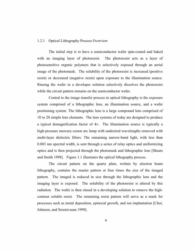
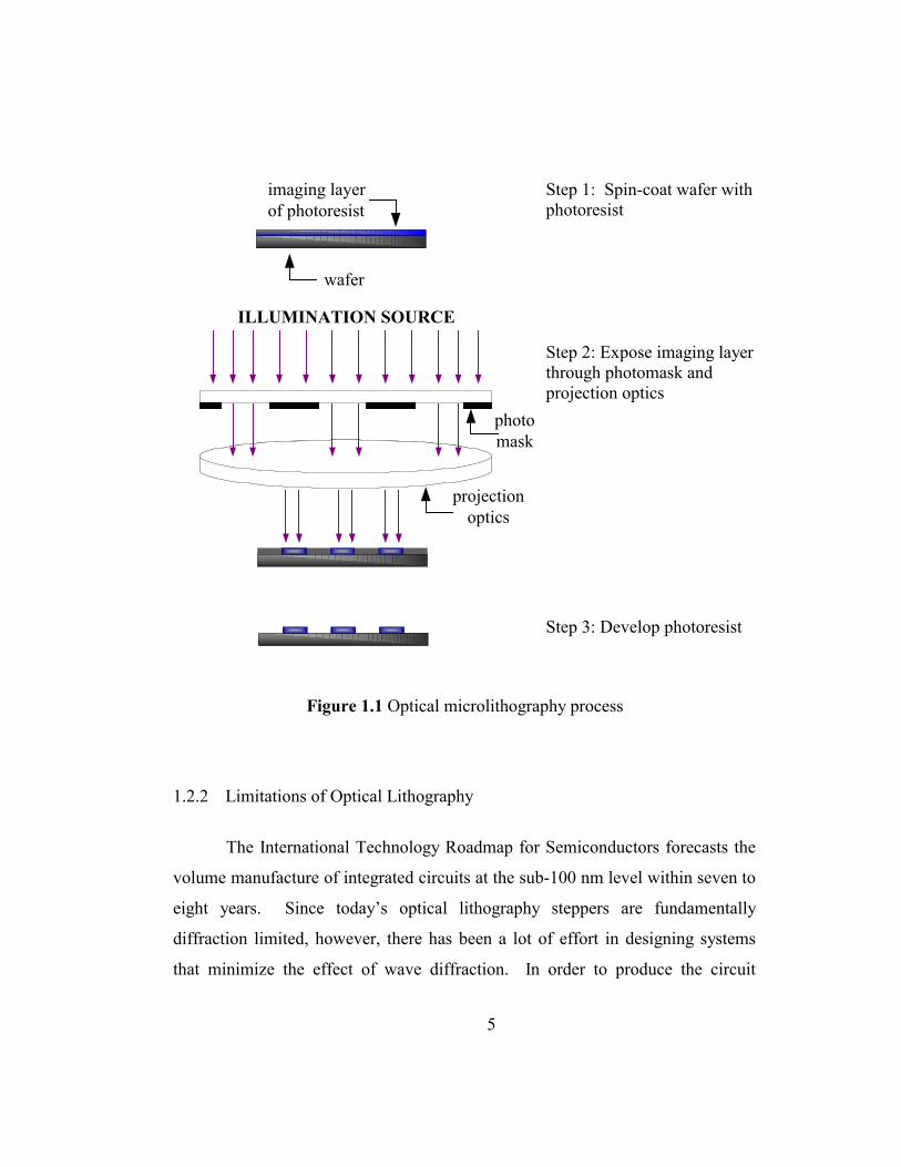
1.2.1 Optical Lithography Process Overview

The initial step is to have a semiconductor wafer spin-coated and baked

with an imaging layer of photoresist. The photoresist acts as a layer of

photosensitive organic polymers that is selectively exposed through an aerial

image of the photomask. The solubility of the photoresist is increased (positive

resist) or decreased (negative resist) upon exposure to the illumination source.

Rinsing the wafer in a developer solution selectively dissolves the photoresist

while the circuit pattern remains on the semiconductor wafer.

Central to the image transfer process in optical lithography is the exposure

system comprised of a lithographic lens, an illumination source, and a wafer

positioning system. The lithographic lens is a large compound lens comprised of

10 to 20 simple lens elements. The lens systems of today are designed to produce

a typical demagnification factor of 4×. The illumination source is typically a

high-pressure mercury-xenon arc lamp with undesired wavelengths removed with

multi-layer dielectric filters. The remaining narrow-band light, with less than

0.003 nm spectral width, is sent through a series of relay optics and uniformizing

optics and is then projected through the photomask and lithographic lens [Sheats

and Smith 1998]. Figure 1.1 illustrates the optical lithography process.

The circuit pattern on the quartz plate, written by electron beam

lithography, contains the master pattern at four times the size of the imaged

pattern. The imaged is reduced in size through the lithographic lens and the

imaging layer is exposed. The solubility of the photoresist is altered by this

radiation. The wafer is then rinsed in a developing solution to remove the high-

contrast soluble resist. The remaining resist pattern will serve as a mask for

processes such as metal deposition, epitaxial growth, and ion implantation [Choi,

Johnson, and Sreenivasan 1999].

5

ILLUMINATION SOURCE

photomask

projectionoptics

imaging layerof photoresist

wafer

Step 1: Spin-coat wafer with photoresist

Step 2: Expose imaging layer through photomask and projection optics

Step 3: Develop photoresist

Figure 1.1 Optical microlithography process

1.2.2 Limitations of Optical Lithography

The International Technology Roadmap for Semiconductors forecasts the

volume manufacture of integrated circuits at the sub-100 nm level within seven to

eight years. Since today’s optical lithography steppers are fundamentally

diffraction limited, however, there has been a lot of effort in designing systems

that minimize the effect of wave diffraction. In order to produce the circuit

6

patterns to the desired specifications, the design of the lens system has very tight

tolerances, which can cause the equipment costs to quickly escalate.

The resolution limit of an optical projection system is governed by the

Rayleigh formula. This states that the numerical aperture of the lens, the

wavelength of light, and the chemical development process determine the

minimum line width that a stepper can print [Thompson, Willson, and Bowen

1994].

AW N

kL λ= [1.1]

where LW is the minimum printable line width (nm), NA is the numerical aperture

of the lens in the stepper, k is the factor describing the photoresist development

process, and λ is the wavelength of the exposure source (nm).

The minimum printable line width can be reduced by 1) increasing the

numerical aperture, 2) improving the processing of the resists, or 3) decreasing

the wavelength of the source illumination. The design of lens systems has seen

an increase in the NA from 0.2 to about 0.73. The proportionality constant k is a

dimensionless number, which is as low as 0.4 for complex multi-layer resist

processes along with phase shift masking to 0.8 for standard resist processes.

Each generation of microlithography technology has incrementally improved line

resolution by incorporating these hardware and process enhancements along with

reducing the wavelength of exposing source.

Many of today’s steppers use 248 nm DUV light and there is currently a

move to 193 nm argon fluoride excimer laser systems with 157 nm systems in

development. Exposure systems with even shorter wavelengths such as x-ray (λ

≈ 1 nm) and extreme ultraviolet (EUV or soft x-ray, λ ≈ 13 nm) are being

7

developed in efforts to reduce current line widths. X-ray and EUV offer an order

of magnitude potential improvement in line widths.

While some of the processes currently in development have demonstrated

the ability to resolve sub-100 nm features in the laboratory, there are technical

and cost considerations that must be overcome to realize their potential benefits.

These processes require optical exposure systems that are rare and expensive.

Also, x-ray lithography requires a helium atmosphere and x-ray masks have

stability problems. Furthermore, these processes have throughput problems. The

effects of wave diffraction, interference, resist sensitivity, and standing wave

effects limit these optical lithography techniques [Chou, Krauss, and Renstrom

1996]. Furthermore, there is the problem of resist transparency as materials that

are transparent to DUV light are opaque to EUV and x-ray regions. With many of

these issues unresolved, it is near certainty that optical methods will not be

adequate for nanoscale (below 100 nm) lithography [Whidden et al. 1996].

High-energy particle lithography schemes such as electron beam (E-beam

direct write/project) and ion beam lithography that have been used to produce

high-resolution patterns, and is used to write and repair photomasks. However,

for wafer processing, they have problems with cost and throughput. These

systems operate serially and cannot maintain the level of throughput required for

economic manufacture of circuits. Furthermore, there exist proximity effects due

to elastic and inelastic particle collisions. These are referred to as forward

scattering in the photoresist and backscattering from the substrate. These

fundamental technical challenges and high cost clearly necessitate the search for

low cost, high-throughput alternatives to optical lithography. SFIL is one such

process that has demonstrated the generation of sub 100 nm features.

8

1.3 STEP AND FLASH IMPRINT LITHOGRAPHY

Step and Flash Imprint Lithography is an innovative, high-throughput,

low cost alternative to optical lithography. SFIL can potentially generate circuit

patterns with sub-100 nm line widths without the use of projection optics

[Colburn et al 1999] and features as small as 60 nm wide have been previously

demonstrated [Choi, Johnson, and Sreenivasan 1999]. SFIL relies mainly on

chemical and mechanical processes to transfer patterns from a quartz template to

a silicon wafer substrate. The use of a low viscosity liquid etch barrier layer

differentiates SFIL from other imprint lithography techniques. The following

section provides an overview of the SFIL process. Then some of the current

challenges faced by SFIL researchers are discussed. For references to other

imprint processes under development, consult [Chou, Krauss, and Renstrom

1996], [Haisma et al. 1996], [Wang et al. 1997], and [Whidden et al. 1996].

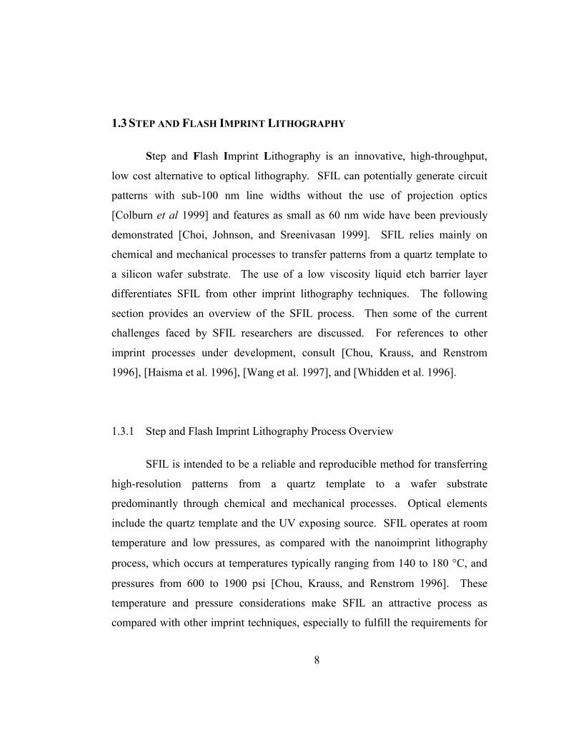
1.3.1 Step and Flash Imprint Lithography Process Overview

SFIL is intended to be a reliable and reproducible method for transferring

high-resolution patterns from a quartz template to a wafer substrate

predominantly through chemical and mechanical processes. Optical elements

include the quartz template and the UV exposing source. SFIL operates at room

temperature and low pressures, as compared with the nanoimprint lithography

process, which occurs at temperatures typically ranging from 140 to 180 °C, and

pressures from 600 to 1900 psi [Chou, Krauss, and Renstrom 1996]. These

temperature and pressure considerations make SFIL an attractive process as

compared with other imprint techniques, especially to fulfill the requirements for

9

an overlay scheme in multi-layered circuits. High temperatures and pressure can

lead to technical difficulties in accurate overlay for multi-layered circuits.

SFIL uses no projection optics and, as with other imprint processes, one

could best describe SFIL as a micro-molding process. The traditional photomask

has been replaced by a topographical template, which contains the circuit pattern

generated by direct write E-beam lithography. The template acts as the master

pattern for the etch barrier layer. The key difference between SFIL and other

imprint lithography techniques is the use of the liquid etch barrier layer. The etch

barrier layer is a low viscosity, photopolymerizable formulation containing

organosilicon precursors [Colburn et al 1999]. This low viscosity eliminates the

need for high temperatures and pressures to achieve the thin films desired for

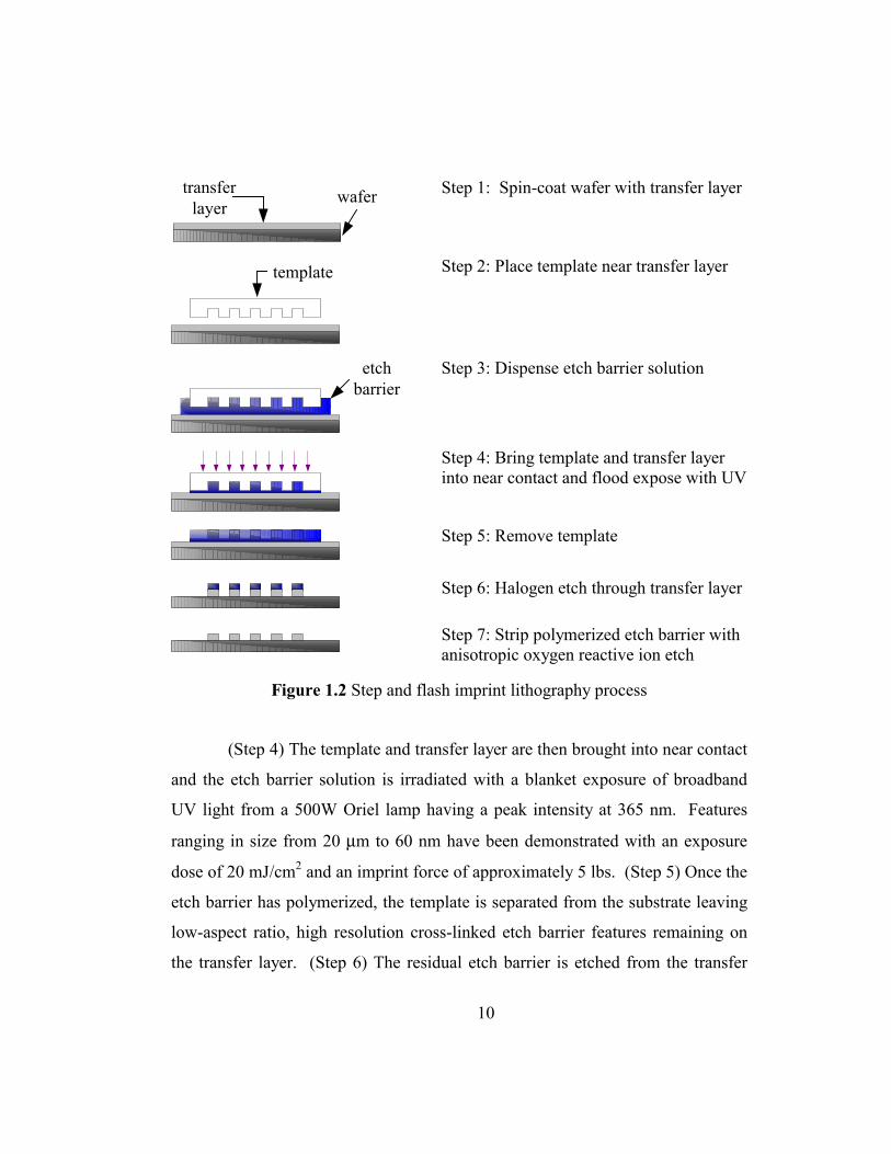
patterning. Figure 1.2 illustrates the SFIL process.

(Step 1) First, an organic transfer layer is spin-coated on a silicon wafer.

This transfer layer adheres to both the silicon wafer and etch barrier layer and

functions as a planarization layer during imprinting while providing high etch rate

selectivity during the device etch step. (Step 2) Next, a quartz template bearing

the relief image of the circuit is brought into proximity of the transfer layer and

wafer. The template must be easily wetted by the etch barrier solution, and it

must easily release the polymerized etch barrier once it has been exposed. In

order to fulfill these requirements, the template is treated with a release layer to

modify its surface chemistry. (Step 3) Once the template is brought near the

wafer, a micro-fluidic dispensing system dispenses a specific pattern of the

photopolymerizable, organosilicon etch barrier fluid. The fluid the fills the gap

between the template and transfer layer via a squeeze film effect and capillary

action.

10

wafertransferlayer

Step 1: Spin-coat wafer with transfer layer

template

Step 2: Place template near transfer layer

etchbarrier

Step 3: Dispense etch barrier solution

Step 4: Bring template and transfer layer into near contact and flood expose with UV

Step 5: Remove template

Step 6: Halogen etch through transfer layer

Step 7: Strip polymerized etch barrier with anisotropic oxygen reactive ion etch

Figure 1.2 Step and flash imprint lithography process

(Step 4) The template and transfer layer are then brought into near contact

and the etch barrier solution is irradiated with a blanket exposure of broadband

UV light from a 500W Oriel lamp having a peak intensity at 365 nm. Features

ranging in size from 20 µm to 60 nm have been demonstrated with an exposure

dose of 20 mJ/cm2 and an imprint force of approximately 5 lbs. (Step 5) Once the

etch barrier has polymerized, the template is separated from the substrate leaving

low-aspect ratio, high resolution cross-linked etch barrier features remaining on

the transfer layer. (Step 6) The residual etch barrier is etched from the transfer

11

layer using a halogen plasma etch. (Step 7) Finally an anisotropic oxygen

reactive ion etch is used to transfer a high aspect ratio image to the transfer layer.

These high aspect ratio features in the transfer layer can then be used as a mask

for transferring the features into the substrate as in traditional lithography, i.e.

metal deposition, etc.

1.3.2 Challenges to Step and Flash Imprint Lithography

In developing the SFIL process, researchers face a number of important

technical challenges. An important aspect of the research is in the realm of

mechanical engineering, which involves developing a step and repeat machine to

implement the process with active control of the orientation stages for parallel

alignment of the template with the wafer substrate. This machine would bring the

template into the proximity of the transfer layer through a coarse z-axis actuation

stage. Then it would dispense the etch barrier solution in the specific pattern

using a micro-liter fluid dispensing system. Next, it would bring the template into

contact with the transfer layer using high-resolution actuators. Finally, it would

illuminate the etch barrier through the backside of the template. A key issue in

the machine development is to understand the interaction between the quartz

template, the thin-film etch barrier layer, and the wafer substrate.

Once the etch barrier fluid fills the gap between the template and the

transfer layer, the template must be pushed towards the wafer in order to

minimize the thickness of the remaining etch barrier base layer. Ideally, the base

layer would be nonexistent in the final imprint process as the etch process that is

used to transfer the image to the transfer layer requires minimal or nonexistent

residual base layer. However, this is not practical in the actual implementation as

12

the etch barrier fluid has an infinite resistance as the base layer thickness

asymptotically reaches zero. The residual etch barrier base layer requires a more

complex etching process. The thickness of the residual base layer should be

uniform and less than the height of the imprinted features (typically 100 nm) in

order to maintain high image fidelity during the etch process. With an acceptable

base layer thickness, a preliminary etching step can eliminate the base layer

without affecting the quality of the process. If the base layer is too thick, the

preliminary etching step cannot eliminate the base layer while maintaining the

feature geometry accurately [Choi, Johnson, And Sreenivasan, 1999].

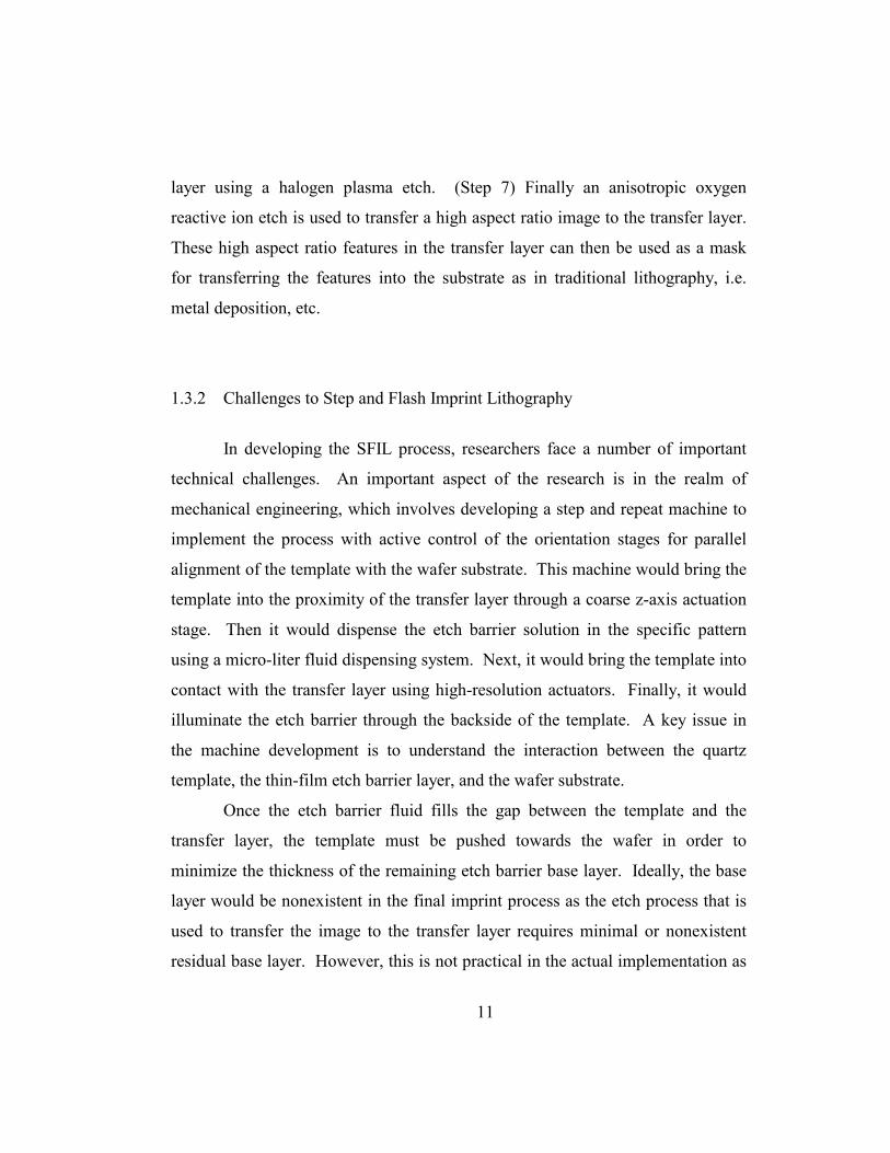
Therefore, it is desirable to achieve a high line height to base layer ratio as

illustrated in Figure 1.3. Since the etch barrier is exposed by a blanket dosage of

UV radiation, the entire layer of etch barrier is polymerized and the etching

process strips is able to completely strip away the thinner areas of the etch barrier

material in the trenches, i.e. the base layer, and leave the thicker areas, i.e. the

lines.

(a) high height ratio, desirable (b) low height ratio, undesirable

Figure 1.3 Ratio of line height to base layer thickness

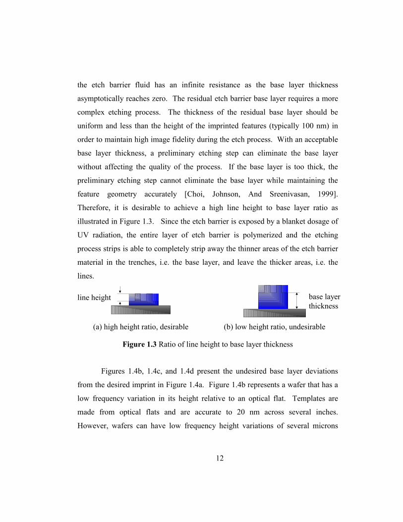
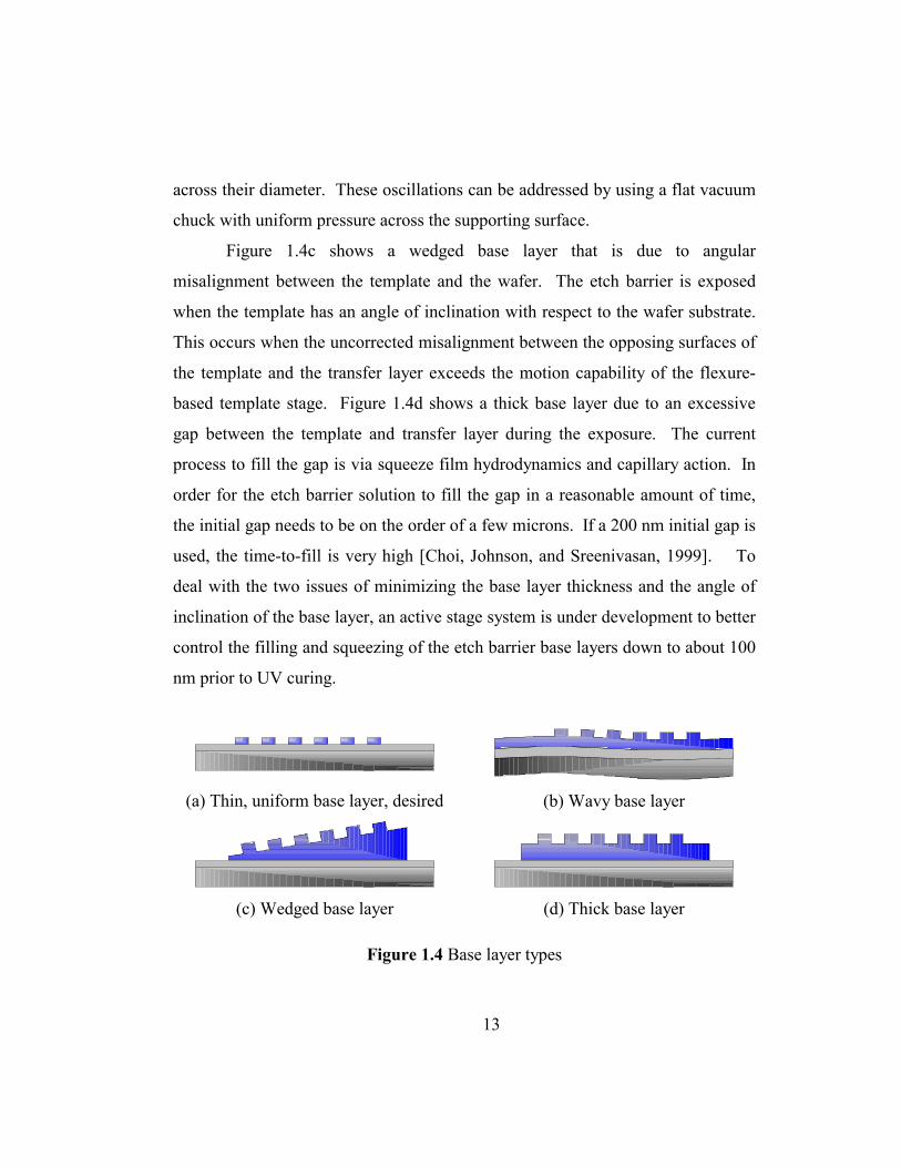
Figures 1.4b, 1.4c, and 1.4d present the undesired base layer deviations

from the desired imprint in Figure 1.4a. Figure 1.4b represents a wafer that has a

low frequency variation in its height relative to an optical flat. Templates are

made from optical flats and are accurate to 20 nm across several inches.

However, wafers can have low frequency height variations of several microns

line height base layer thickness

13

across their diameter. These oscillations can be addressed by using a flat vacuum

chuck with uniform pressure across the supporting surface.

Figure 1.4c shows a wedged base layer that is due to angular

misalignment between the template and the wafer. The etch barrier is exposed

when the template has an angle of inclination with respect to the wafer substrate.

This occurs when the uncorrected misalignment between the opposing surfaces of

the template and the transfer layer exceeds the motion capability of the flexure-

based template stage. Figure 1.4d shows a thick base layer due to an excessive

gap between the template and transfer layer during the exposure. The current

process to fill the gap is via squeeze film hydrodynamics and capillary action. In

order for the etch barrier solution to fill the gap in a reasonable amount of time,

the initial gap needs to be on the order of a few microns. If a 200 nm initial gap is

used, the time-to-fill is very high [Choi, Johnson, and Sreenivasan, 1999]. To

deal with the two issues of minimizing the base layer thickness and the angle of

inclination of the base layer, an active stage system is under development to better

control the filling and squeezing of the etch barrier base layers down to about 100

nm prior to UV curing.

(a) Thin, uniform base layer, desired (b) Wavy base layer

(c) Wedged base layer (d) Thick base layer

Figure 1.4 Base layer types

14

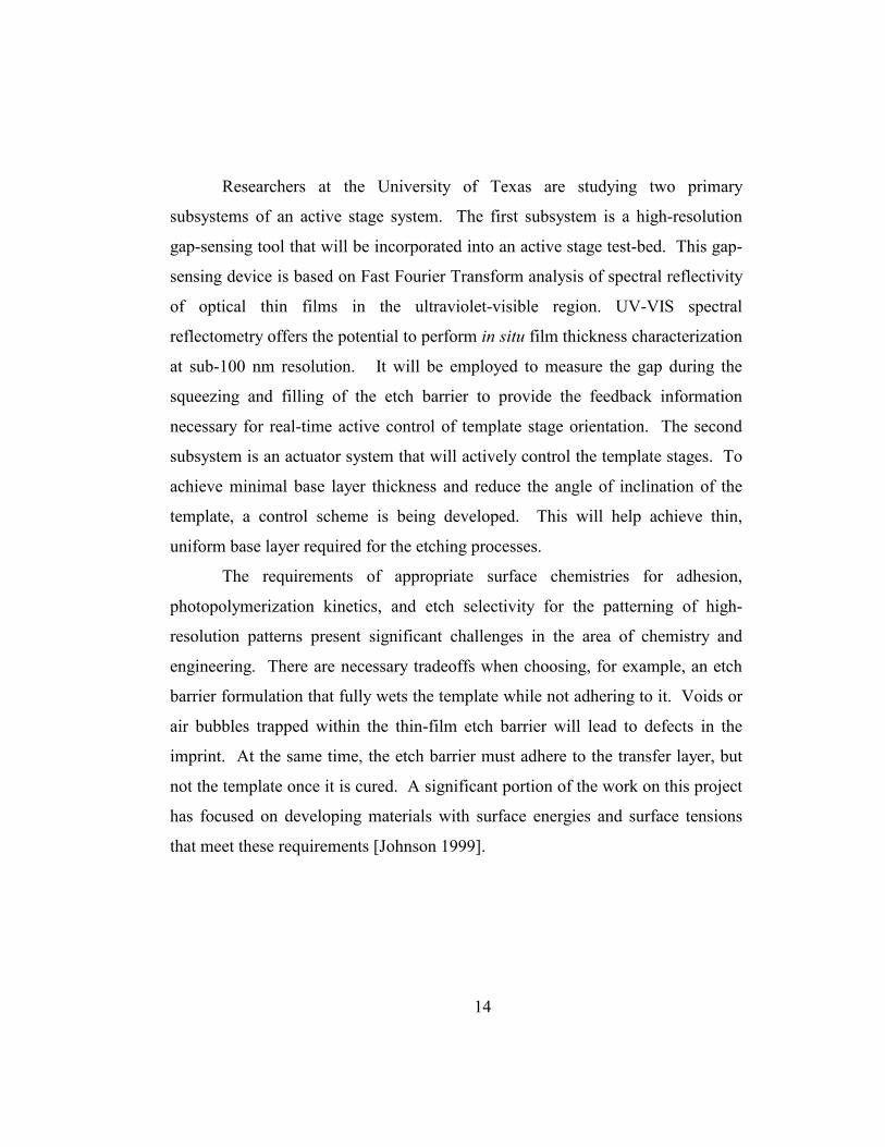
Researchers at the University of Texas are studying two primary

subsystems of an active stage system. The first subsystem is a high-resolution

gap-sensing tool that will be incorporated into an active stage test-bed. This gap-

sensing device is based on Fast Fourier Transform analysis of spectral reflectivity

of optical thin films in the ultraviolet-visible region. UV-VIS spectral

reflectometry offers the potential to perform in situ film thickness characterization

at sub-100 nm resolution. It will be employed to measure the gap during the

squeezing and filling of the etch barrier to provide the feedback information

necessary for real-time active control of template stage orientation. The second

subsystem is an actuator system that will actively control the template stages. To

achieve minimal base layer thickness and reduce the angle of inclination of the

template, a control scheme is being developed. This will help achieve thin,

uniform base layer required for the etching processes.

The requirements of appropriate surface chemistries for adhesion,

photopolymerization kinetics, and etch selectivity for the patterning of high-

resolution patterns present significant challenges in the area of chemistry and

engineering. There are necessary tradeoffs when choosing, for example, an etch

barrier formulation that fully wets the template while not adhering to it. Voids or

air bubbles trapped within the thin-film etch barrier will lead to defects in the

imprint. At the same time, the etch barrier must adhere to the transfer layer, but

not the template once it is cured. A significant portion of the work on this project

has focused on developing materials with surface energies and surface tensions

that meet these requirements [Johnson 1999].

15

1.4 THESIS

For SFIL to become a practical technology, real-time control strategies

must be developed to in order to generate thin, parallel base layers. To better

understand the requirements for the specifications of an active stage system

capable of delivering thin, parallel base layers, the fluid film interaction with the

template and wafer has been investigated for this thesis. A squeeze film model

of the fluid film was used to develop the analytical equations for the fluid

pressure, which are a function of the template geometry, orientation, and

velocities. For a given template geometry, the pressure is then a function of

orientation and velocity.

),,,,( θθ DDhhxpp = . [1.2]

The solution for the pressure was obtained from the Reynolds equation,

which is the fundamental equation in fluid film lubrication theory. The pressure

was then integrated over the spatial domain to obtain analytical solutions for the

damping force and torque generated by the fluid. Then, a numerical simulation of

the equations of motion for the template assembly was performed to characterize

the dynamics of the mechanical system and its interaction with the etch barrier

layer. Finally, an experiment was designed to scientifically quantify the squeeze

film dynamics of the etch barrier layer. An improved understanding of the

squeeze film mechanics is derived from the combined efforts of theoretical,

numerical, and experimental analysis.

The remainder of this thesis has been organized into six chapters. Chapter

2 reviews the theoretical background on modeling the squeeze film effects of the

etch barrier layer. The model assumptions are explained and a derivation for the

Reynolds equations is given. Boundary conditions for specific geometries were

applied to obtain appropriate analytical solutions. Chapter 3 discusses the active

16

stage development. Design requirements and implementation for major

subsystems in the active stage are considered. Chapter 4 gives the theory and

implementation details of a gap sensing system based on Fast Fourier Transforms

of the spectral reflectivity of thin films. Chapter 5 presents the numerical

simulation results and an interpretation in the context of SFIL process and

machine development. Chapter 6 discusses the design of experiments to validate

the model and provide insight into what happens during the squeezing process.

Experimental results are correlated to the results from numerical simulations of

the squeezing process. Chapter 7 summarizes this research, poses possible

extensions, and notes the major contributions of this research to SFIL

development.

17

Chapter 2: Theoretical Analysis

The first step taken to model a physical system is to understand the

physics of the system. The SFIL system considered here is comprised of a

quartz template (T), a photosensitive, etch barrier fluid (F), and a flat wafer

substrate supported by a vacuum chuck (W). The TFW system has been modeled

as a squeeze film flow between two flat surfaces. Different assumptions about the

geometry of the system lead to slightly modified analytic equations for the

pressure distribution due to the liquid etch barrier.

2.1 INTRODUCTION

The development of a reliable, high-throughput step and flash imprint

lithography process requires an improved understanding of the interaction

between the etch barrier layer and the flexure stages, which orient the template.

The step required to expel the excess liquid etch barrier between the template and

the wafer substrate is a critical and rate-limiting step in the SFIL process. The

etching process requires that the base layer thickness be on the order of the

average feature height, which is about 200 nm in the current process. For

throughput to be competitive with industry standard processes, this step should be

completed in about 0.5 seconds because time must also be allocated for

translation of the x-y stage, dispensing the etch barrier, and exposing the etch

barrier. In this short time interval, the gap between the template and the substrate

has to be reduced from several microns to 100-200 nm. This also requires that the

orientation misalignment must be less than 0.5 µrad if the difference between the

18

minimum and maximum base layer thickness is to be less than 10%. Due to high

damping forces and mechanical compliance, achieving these results is not trivial.

In order to optimize the design of an active stage system, the following

questions must be answered. 1) What mechanisms are dominant during the filling

process as the liquid etch barrier wets the surface of the template and wafer? 2)

What characterizes the measured imprinting forces of the etch barrier as the

template and wafer are pressed together. Studying the behavior of the etch barrier

layer and its effect on the dynamics of the actuation system will provide insight

into a method for obtaining thin base layers within a reasonable amount of time

from actuation forces that can be achieved by commercially available actuators.

The behavior of the etch barrier can be described by that of squeeze films,

which commonly occur in lubrication theory. It has been observed, in the current

SFIL process using a multi-imprint stepper [Choi, Johnson, and Sreenivasan

1999], that the characteristic imprinting force as a function of time is

approximately a step function. Intuitively, the greater the viscosity of the etch

barrier, the larger the force required to reduce the thickness of the fluid layer; or

alternatively, for a given force more time is required to achieve the desired base

layer thickness. Furthermore, it has been observed that the fluid has very high

resistance at a base layer thickness below 100 nm. From these observations, the

etch barrier has been modeled as a squeeze film lubrication flow.

The lubrication flow of squeeze films has been widely studied in the past

century in the context of tribology applications, where oil is typically the

lubricant. Researchers have examined the effect of roughness on squeeze film

lubrication flow through stochastic models of surface roughness. Assuming

surfaces with known statistical properties, i.e. Gaussian distributions with known

mean and standard deviations, averaged Reynolds equation flow models were

derived [Tripp 1983; Patir and Cheng 1978]. The effects of sinusoidal

19

corrugations on the flow behavior of parallel plate squeeze films have been

studied from a theoretical and numerical perspective [Freeland 2000]. Freeland

developed analytic and numerical solutions for two and three-dimensional

geometries for flows found in both SFIL and nanoimprint lithography. The non-

inertial sinkage of a flat, inclined plate has been thoroughly studied. However,

the effect of the asymmetry in the pressure distribution across the plate was

neglected in computing the sinkage rate [Moore 1964]. Moore proceeded with

the assumption of a pressure distribution, which is a parabola for any section

perpendicular to the directions spanning the plate. This assumption neglects the

corner effects, but is useful in approximating the three-dimensional pressure due

to a specified load condition. In this thesis, the effect of a non-symmetric

pressure variation across a smooth template is treated analytically and applied to a

numerical simulation of the equations of motion for the SFIL machine.

In this chapter, the Reynolds equation has been used to study the case of

a squeeze film flow between a flat, quartz template and flat, rigid wafer substrate.

First a derivation of the incompressible Reynolds equation is given. Next, a

reduced form of the Reynolds equation is considered. The two-dimensional

Reynolds equation can be applied to flow geometries where side leakage can be

neglected in one of the lateral directions; the squeeze film in the y direction can

be considered infinite. The case of an infinite, flat surface that is parallel to a

substrate is presented. This is extended to the case of an infinite, flat surface that

is inclined relative to a substrate. Applying specific boundary conditions,

analytical solutions for the pressure, force, and torque are obtained from the two-

dimensional Reynolds equation.

The analytical solutions to the three-dimensional problem (finite plate

geometry) are reviewed as used as a benchmark for comparing the two-

dimensional solutions. The three-dimensional solution for the case of a parallel

20

square plate with fluid completely filling the gap is considered. Finally, the

closed-form solution to the case of parallel circular plates is presented. The

axisymmetric case has a readily available solution to the problem of a growing

fluid boundary layer.

2.2 THE INCOMPRESSIBLE REYNOLDS EQUATION

The Reynolds equation is the basic equation for fluid lubrication. It

provides a relationship between the thickness of a fluid film and the pressure.

Since the problem of interest is not a traditional lubrication flow, it is a

prerequisite that careful consideration be given to the assumptions used in

modeling the squeeze film effect of the etch barrier liquid. The characteristic

length for the expulsion step in the SFIL process is on the order of hundreds of

nanometers. A desired final base layer thickness of 100 - 200 nm is virtually at

the limit of contacting plates in most traditional engineering contexts. For a fluid

layer at these thicknesses, does the assumption of the fluid as a continuum remain

valid? An empirical criterion such as the Stribeck Curve2 shows that for films

above about 10 nm, the lubricant film behavior can be described by bulk,

continuum properties [Bhushan 1995]. Also, at this scale of motion, the effect

of van der Waals forces could become important as compared with the pressure

forces from the bulk fluid and the external forces. The pressures created by the

van der Waals forces are proportional to

36 avg

VW hAPπ

∝ or 3 6 appliedavg P

Ah π∝ [2.1]

2 Refer to page 292 of the Handbook of Micro/Nanotribology by Bharat Bhushan.

21

where A is the Hamaker constant (~ 10-20 J), havg is the average distance between

the plates (m), and Pappplied is the applied pressure (Pa).

Assuming the applied pressures on the order of 1 psi, havg is about 4 nm when

van der Waals forces are on the same order as the pressures of interest [Freeland

2000]. Also, Moore documents that it has been agreed that molecular influence

can extend outward from a surface no more than 0.5 µin (13 nm). A base layer

thickness of approximately 100 nm, well above these limits of continuum fluid

mechanics, justifies a few of the following assumptions.

In deriving the Reynolds equation, the assumptions that are to be made must

be considered:

1. Body forces are neglected, i.e. van der Waals forces.

2. The pressure is constant through the thickness of the film. Since the

thickness of the films considered here are about ten microns or smaller,

while the length scales in the plane of the template are measured in

centimeters, it is reasonable to assume that 0=∂∂

zp .

3. There is no slip at the boundaries. There has been much work on this and

it is universally accepted [Cameron 1976].

4. The fluid is Newtonian, i.e. zu∂∂= µτ . Shear stress is proportional to the

rate of shear strain. This assumption is valid when the lubrication is in the

bulk regime (minimum film thickness above 10 nm).

5. The flow is laminar. The Reynolds number based on gap height is less

than one for the range of gap heights and velocities. 1Re <<h

6. Fluid inertia is neglected since the kinematic viscosity is large and the

length scale is small.

22

7. The fluid is assumed incompressible since the etch barrier and water are

liquids.

8. The viscosity can be considered constant throughout the fluid layer since

the SFIL process operates at room temperatures.

9. The flow is quasi-steady. This assumption asserts that the velocity and

pressure fields adjust instantaneously to the movements of the boundary.

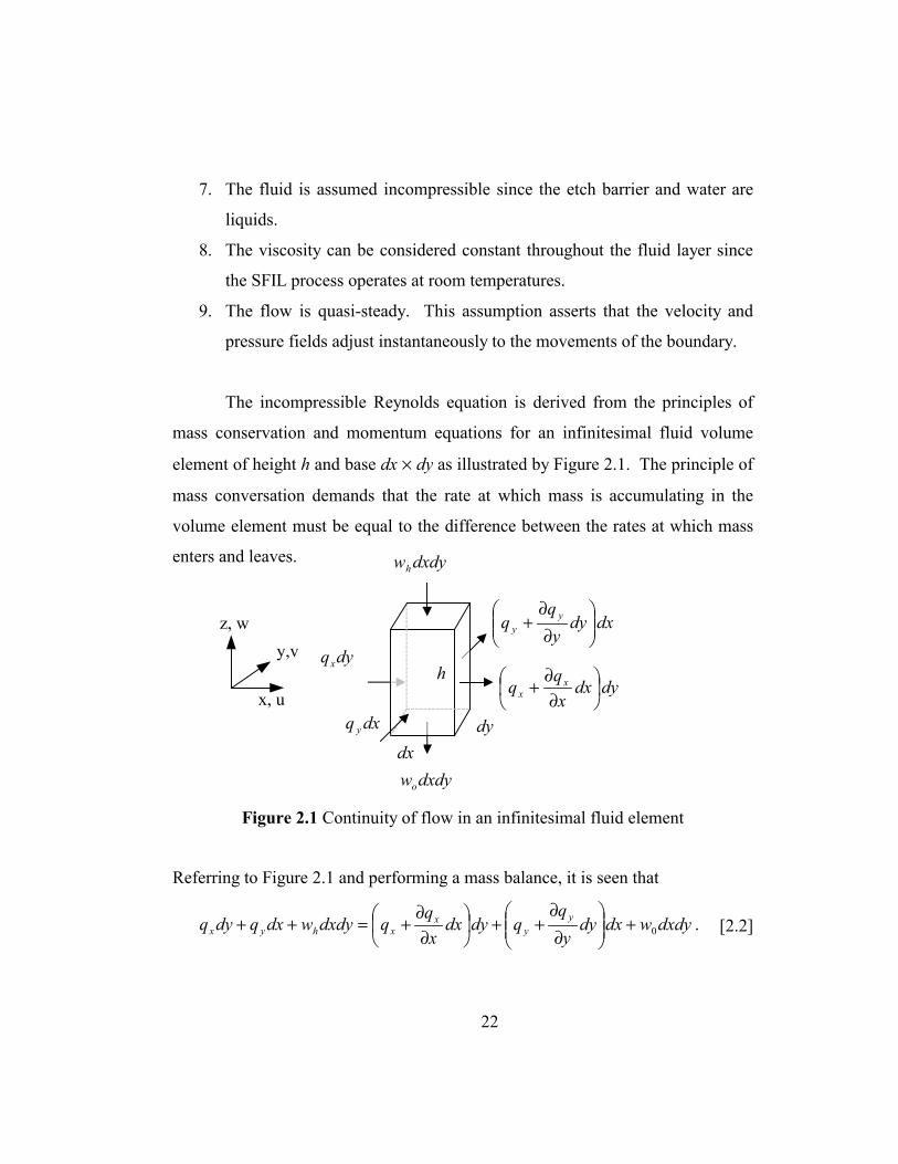
The incompressible Reynolds equation is derived from the principles of

mass conservation and momentum equations for an infinitesimal fluid volume

element of height h and base dx × dy as illustrated by Figure 2.1. The principle of

mass conversation demands that the rate at which mass is accumulating in the

volume element must be equal to the difference between the rates at which mass

enters and leaves.

x, u

y,vz, w

Figure 2.1 Continuity of flow in an infinitesimal fluid element

Referring to Figure 2.1 and performing a mass balance, it is seen that

dxdywdxdy

yq

qdydxx

qqdxdywdxqdyq y

yx

xhyx 0+

∂∂++

∂∂+=++ . [2.2]

dyqx

dydxx

qq xx

∂∂+

dxq y

dxdyy

qq y

y

∂∂+

dxdywo

dxdywh

h

dy dx

23

The left hand side of equation 2.2 is the volume flow rate into the fluid element

and the right hand side is the volume flow rate out of the fluid element.

Canceling common terms and factoring appropriately gives

( ) 00 =

−+∂∂+

∂∂

dxdywwy

qx

qh

yx . [2.3]

Note that the term dxdy is arbitrary and nonzero and that the template and wafer

surfaces are impermeable, therefore ( )thwwh ∂∂=− 0 . Thus, equation 2.3 is written

more succinctly as,

0=

∂∂+⋅∇

thq . [2.4]

This is the continuity equation for incompressible flow, where ∇ is the two-

dimensional gradient operator and the latter term is the average rate at which the

template approaches the wafer.

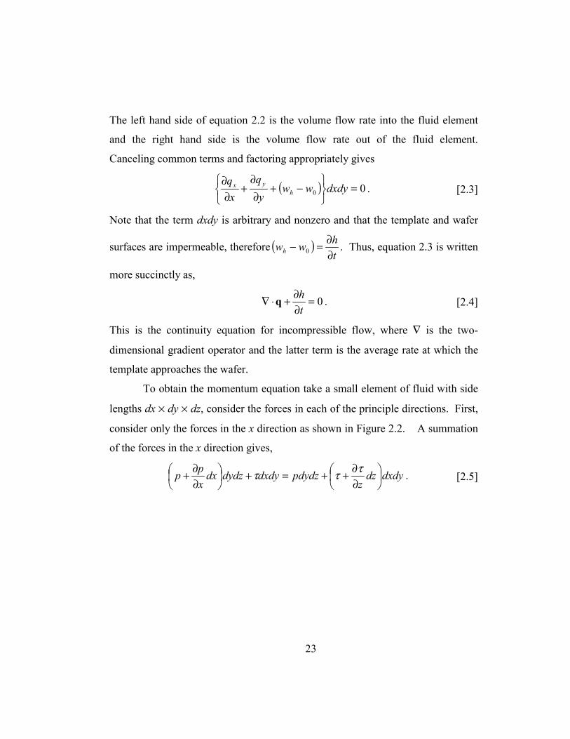
To obtain the momentum equation take a small element of fluid with side

lengths dx × dy × dz, consider the forces in each of the principle directions. First,

consider only the forces in the x direction as shown in Figure 2.2. A summation

of the forces in the x direction gives,

dxdydz

zpdydzdxdydydzdx

xpp

∂∂++=+

∂∂+ τττ . [2.5]

24

x, u

y,vz, w

Figure 2.2 Force equilibrium of an infinitesimal fluid element

Collecting like terms, this can be simplified

zx

p∂∂=

∂∂ τ . [2.6]

Recall that the fluid is assumed Newtonian, thus

∂∂

∂∂=

∂∂

zu

zxp µ . [2.7]

Similar reasoning is applied in the y direction to obtain

∂∂

∂∂=

∂∂

zv

zyp µ . [2.8]

Recalling that 0=∂∂

zp from assumption no. 2, a balance of the pressure and shear

forces on an equilibrium element yields the momentum equation.

p

z∇=

∂∂

2

2u [2.9]

where yx eeu vu += .

Consider equation 2.7 further. This can be integrated since p is not a

function of z, thus

1Cz

xp

zu +∂∂=

∂∂µ . [2.10]

A further integration gives

dydzdxxpp

∂∂+

dxdydzz

∂∂+ ττ

pdydz

dxdyτ

25

21

2

2CzCz

xpu ++∂∂=µ . [2.11]

The boundary conditions due to the no slip condition is the speed of the surface,

so on, hz = 1Uu =

and on 0=z 2Uu =

where U1 and U2 are the two surface speeds.

Substituting these into equation 2.11 produces 22 UC µ= and

( )2

211

hxp

hUUC

∂∂−

−=µ . The velocity in the x direction at any point in z in the

film is given by

( ) ( ) 2212

2U

hzUUzhz

xpu +−+−∂∂=µ

. [2.12]

The velocity gradient is

( )h

UUhzx

pzu 1

2 21 −+

−∂∂=

∂∂

µ. [2.13]

The integral ∫hudz

0equals qx, the flow rate in the x direction per unit width of y.

Integrating equation 2.12 gives

( )

h

x zUh

zUUhzzx

pq0

2

2

21

23

2232+−+

−

∂∂=µ

. [2.14]

Putting in the limits and simplifying, the result is

( )212 21

3 hUUxphqx ++∂∂−=µ

. [2.15]

Following the same procedure for y it is easily found that

( )212 21

3 hVVyphq y ++∂∂−=µ

. [2.16]

26

where V1 and V2 correspond to U1 and U2.

Going back to the continuity equation and replacing the terms qx and qy in

equation 2.3 by (2.15) and (2.16) gives

( ) ( ) 0

122122

3

21

3

21 =∂∂+

∂∂−+

∂∂+

∂∂−+

∂∂

th

yphhVV

yxphhUU

x µµ. [2.17]

This can be somewhat simplified to read

( ) ( )

∂∂++

∂∂++

∂∂=

∂∂

∂∂+

∂∂

∂∂

thhVV

yhUU

xyph

yxph

x26 2121

33

µµ. [2.18]

This is the Reynolds equation in three dimensions. There exist no general closed-

form solutions to this generalized form of the Reynolds equation. The following

section simplifies the equation 2.18 with the appropriate model assumptions.

2.3 THE TWO-DIMENSIONAL REYNOLDS EQUATION 2.3.1 Derivation of the Two-Dimensional Reynolds Equation

The generalized form of Reynolds equation from equation 2.18 can be

reduced to a two-dimensional form, which can be applied for certain plate

geometries and boundary conditions. For relatively low interface pressures in

hydrodynamic lubrication, the viscosity of fluids can be assumed to be constant

[Bhushan 1999]. Also, if the motion is restricted to normal approach such that

sliding velocities are zero ( )02121 ==== VVUU , equation 2.18 reduces to

th

yph

yxph

x ∂∂=

∂∂

∂∂+

∂∂

∂∂ µ1233 [2.19]

In the process of expelling the excess etch barrier, the side motion of the

template relative to the wafer is negligible due to the design of the flexure stages,

27

which are selectively compliant. In the multi-imprint machine, these flexures are

passive compliant and allow α-β rotations, as shown in Figure 2.3, and z

translation while minimizing γ rotations and x-y translations.

The selective compliance of the distributed flexure allows the flexure to

self-correct any orientation alignment within its range of motion to minimize the

base layer wedge profile when the etch barrier is squeezed towards the edges of

the template. During the separation step excessive lateral displacements may

destroy transferred images, therefore an important design criterion for the

orientation stages is to minimize the motions that would cause catastrophic

defects in the UV-exposed etch barrier. Thus, the modeled fluid pressures are

generated from a pure squeeze action and the first two terms on the right hand

side of equation 2.18 disappear.

Figure 2.3 Two flats showing orientation alignments3

The template is treated as infinite in the y direction and only the middle of

the template along the x direction is considered. This is equivalent to neglecting

side leakage so that all y derivatives are zero. The two-dimensional Reynolds

equation becomes

3 Figure taken from Choi et al 2000.

x,α

y,β

z,γinitial template

substrate

aligned template

28

th

dxdph

dxd

∂∂=

µ123 . [2.20]

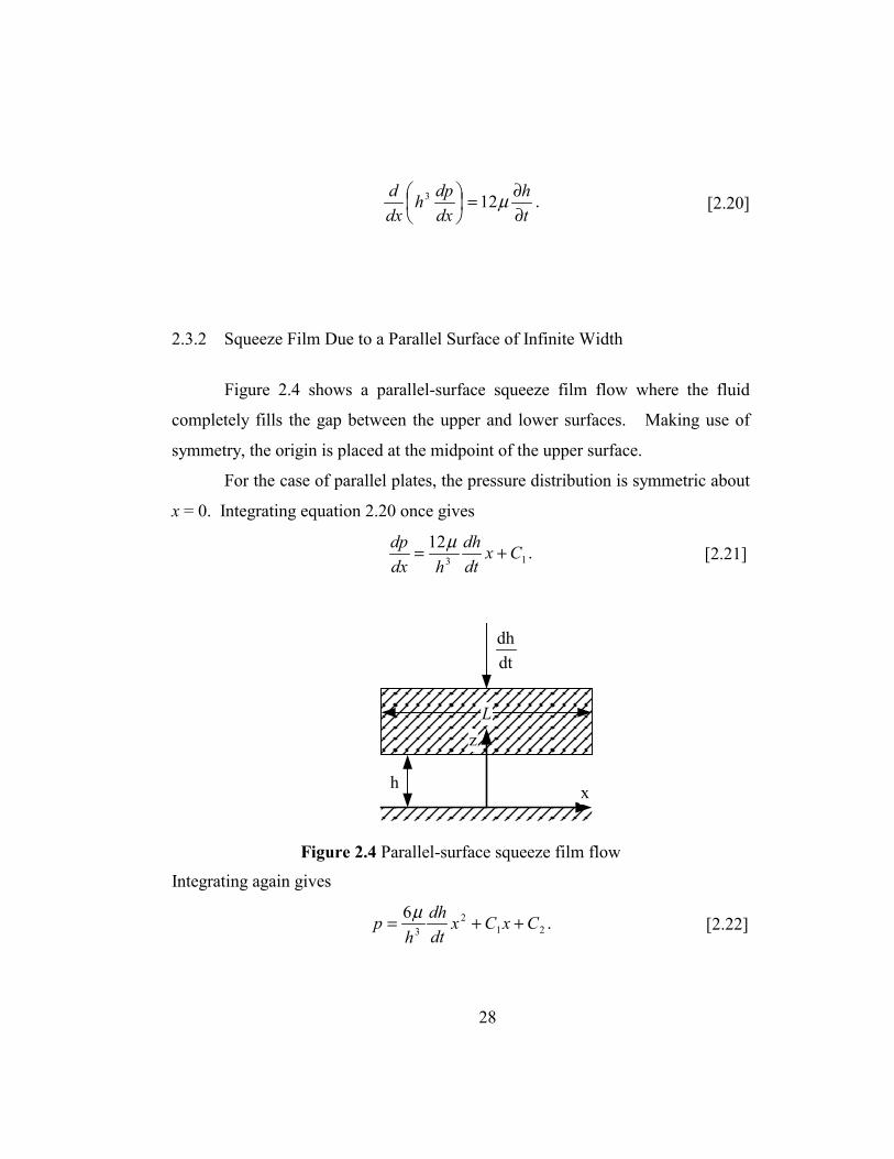
2.3.2 Squeeze Film Due to a Parallel Surface of Infinite Width

Figure 2.4 shows a parallel-surface squeeze film flow where the fluid

completely fills the gap between the upper and lower surfaces. Making use of

symmetry, the origin is placed at the midpoint of the upper surface.

For the case of parallel plates, the pressure distribution is symmetric about

x = 0. Integrating equation 2.20 once gives

13

12 Cxdtdh

hdxdp += µ . [2.21]

h x

Lz

dtdh

Figure 2.4 Parallel-surface squeeze film flow

Integrating again gives

21

23

6 CxCxdtdh

hp ++= µ . [2.22]

29

The boundary conditions are 0=p when 2Lx ±= . From the boundary

conditions, 01 =C and dtdh

hLC 3

2

2 46µ−= . Substituting for C1 and C2 gives

( ) ( )223 4

23 Lx

dtdh

hxp parallel −= µ . [2.23]

The pressure distribution is parabolic and symmetric about ( )0=x . For parallel

plates the normal damping force per unit width is simply

dtdh

hLdxxpf

L

Lparallel 3

32

2

)( µ−== ∫−

[2.24]

From equation 2.24, it is observed that the fluid layer generates large

damping forces that scale as 3

1h

and is directly proportional to both the approach

velocity of the template and the viscosity of the fluid.

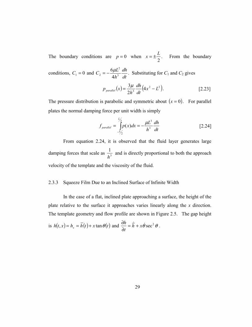
2.3.3 Squeeze Film Due to an Inclined Surface of Infinite Width

In the case of a flat, inclined plate approaching a surface, the height of the

plate relative to the surface it approaches varies linearly along the x direction.

The template geometry and flow profile are shown in Figure 2.5. The gap height

is ( ) ( ) ( )txthhxth x θtan, +== and θθ 2secDD xhth +=∂∂ .

30

θhα hβ

x

z

dtdh

L

xα x = 0 xβ

h

Figure 2.5 Inclined-surface squeeze film flow

The height at the midpoint of the template at x = 0 is given by ( )th and the

velocity is ( )thD . The domain is specified on ( ) ( )],[ txtxx βα∈ . The integration

domain grows as a function of time due to the fluid being squeezed out from the

midpoint.

The height of the template at the left and right boundaries

are θαα tanxhhx += and θββ tanxhh += , respectively. The initial conditions

at the boundaries of the flow at x = xα and x = xβ are determined by the volume of

the fluid dispensed and the average height of the template. For example, if the

volume of fluid dispensed is 0.1 µL or 1×10-10 m3, 2/

101 10

Lhd

−×= in meters where

d = αx = xβ. However, the half-length of the template constrains xα and xβ so

that βα xxL ,2≥ . Since the height is a function of x, the integration to obtain the

31

pressure distribution is tedious and only the result follows. Integrating the two-

dimensional Reynolds equation once gives

+

+= 1

22

3 sec2

121 Cxxhhdx

dp

x

θθµ DD . [2.25]

Integrating again gives

( )

+++−= 2

2

3

2

22 2tan43

tansec6

tantan26)(

xx hxhh

hxhhxp θ

θθθµ

θθµ DD

221

tan2ln C

hC

hh

x

x +−

+

θα

[2.26]

For the unsubmerged plate-surface system, meniscus effects at the outer

periphery of the squeeze film, and capillary pressure opposes the squeeze film

pressure [Moore 1965]. Assuming the liquid perfectly wets the surfaces of the

plate and substrate, i.e., zero contact angles, the pressure at the boundary is given

by ( )xh

xp γ2−= . Applying the boundary conditions ( )α

αγ

hxxp 2−== and

( )β

βγ

hxxp 2−== , the integration constants, C1 and C2, are obtained.

θαα tanxhhx += , θββ tanxhhx += , θθθµ

3

2

tansec6 D

=k ,

( ) ( )

+

++

+−=

α

β

β

β

β

β θθ

θµ

x

x

xx hh

hxhh

khxhh

C ln2

tan43tan

tan262

2

221

D

,

( ) ( )θθµθ

α

α

α

α222

2

2 tantan26

2tan43

xx hxhh

hxhhkC +

++−

=D

,

32

( ) ( )2122

22

1

tan2CCPP

hhhh

C xxxx

xx ++−−

= αββα

βα θ, and

θα tan2 21

22xhCCC += .

Equation 2.26 numerically converges to the result of equation 2.23 for a

certain range of small θ, but due to integration of equation 2.25 the limit as θ

tends to zero becomes ill posed and the numerical result becomes unstable for

small θ. However, using a Taylor series expansion of the height h(x) gives a

result that converges to the parallel plate solution for θ = 0. The height is

rewritten as ( )

+= θtan1hxhxh . When the ratio of the wedge height to the

average height is small, i.e. θtanhx << 1, a Taylor approximation can be used for

the term ( )333tan1

11

θhxhh +

= in equation 2.25. Substituting into equation

2.25 the Taylor approximation

−≈ θtan311133 h

xhh

, the resulting pressure

distribution is

+

−+−

= 32

42

3

tan6

sec8

tansec312 xh

hxhh

p θθθθθθµ DDD

2121

128tan

2CxCx

hCh +

−

+

µµθD

[2.27]

where C1 and C2 are given by

( ) ( ) ( )+−−

+−

−+−= 44

2

22

4

1 8tansec3

tan322

αβαβαββα

θθθθ

xxh

PPxxxxh

hC xx

D

33

( ) ( )

−+−

− 2233

2

2tan

6sec

βαβαθθθ xxhxx

hh DDD

+

−+−

−= 32

42

32tan

6sec

8tansec312

βββθθθθθθµ x

hhx

hhPC x

DDD

−

+ ββ µµ

θ xCxh

Ch128

tan2

121D

Equation 2.27 is valid for small values of ( )

θβα tan,max

hxx

. Note that equation

2.27 is a polynomial equation in x. It can be shown that in the limit, as θ

approaches zero, the pressure distribution approaches that of a parallel plate

(equation 2.23).

In Figure 2.6, the pressure distributions for both parallel and nonparallel

plates are presented. The pressure distribution for the case of nonparallel plates is

skewed and generates a torque to correct the deviation of θ from zero. Figure 2.6

shows that for small angles, the pressure distribution is nearly symmetric and that

the location of the maximum pressure moves away from x = 0.

The damping force resulting from the squeeze film pressure is obtained by

the integration of the pressure over the projected area of the wetted portion of the

template. This damping force is given by

∫ ∫=L x

x

dxdyxpf0

)(β

α

. [2.28]

The result of this integration is

( ) ( )+−

−+−

= 44

255

2

3 4tan

24sec

40tansec312

αββαθθθθθθµ xx

hhxx

hhLf

DDD

34

( ) ( ) ( )

−+

−+−

+ αββααβ µµ

θ xxCxxCxxh

Ch2

221331

2424tan

6

D

. [2.29]

-0.4 -0.3 -0.2 -0.1 0 0.1 0.2 0.3 0.4-10

-5

0

5

10

15

20

x, in

Figure 2.6 Two-dimensional pressure distribution

Figure 2.6 shows the two-dimensional pressure along the template for

parallel plates solution from equation 2.23 (solid line), inclined plate solution

from equation 2.26 (dash-dotted line), and inclined plate solution from equation

2.27 (dashed line). Results are for h = 1 µm, h� = –0.5 µm/s, θ = 10 µrad, and

10−=θ� µrad/s with boundary conditions hLh

xp γ22/

101 10 −=

×±=−

. L = 1 inch.

The damping torque is given by

∫ ∫=L b

a

dxdyxxp0

)(τ [2.30]

pres

sure

, psi

35

and the result is

( ) ( )+−

−+−

= 55

266

2

3 5tan

30sec

48tansec312

αββαθθθθθθµτ xx

hhxx

hhL

DDD

( ) ( ) ( )

−+

−+−

+ 222331441

23632tan

8 αββααβ µµθ xxCxxCxx

hChD [2.31]

2.4 THREE-DIMENSIONAL PROBLEM 2.4.1 3D Pressure Distribution for Parallel, Rectangular Plates

In the previous two-dimensional case, the plates were considered to be

infinite in the y direction. In the three-dimensional case, the plate dimensions are

finite. For a flat, rectangular plate moving parallel towards a flat surface with

fluid completely filling the gap, i.e. there is no capillary effect; the pressure

distribution in the squeeze film is relatively complex owing to the introduction of

corner effects and the absence of rotational symmetry. For a rectangular plate of

length L and width B where the shape ratio B/L gives a characteristic shape

factor, ( )LBf , Hays assumed an infinite, double Fourier series solution for the

pressure distribution of the following form

∑∑∞ ∞

=M N

MN NMAp φθ sinsin [2.32]

where [ ]∞= ..., ,5 ,3 ,1 , NM , Lxπθ = and

Byπφ = [Moore 1965]. This satisfies the

zero boundary conditions such that the pressure is the same atmospheric pressure

36

at the plate edges. Freeland obtained the series coefficients, AMN, in the case of a

flat, square template, i.e. B = L. The pressure distribution is given by

( )( )( )( ) ( )( ) −

+

+−+−= ∑

∞

=

12sinh12sinh

112cosh 480

33

2

nyn

nn

dtdh

hLp π

ππ

πµ

( )( ) ( )( )( )312

12sin1 12cosh++

++

nxnyn ππ

[2.33]

When the pressure is integrated with respect to x and y, the force due to the

squeeze film between flat parallel plates is

( )( )( )( ) ( )( )[ ]∑

∞

= −−+

+−+−=

035

4

112cosh12sinh

112cosh48n

nn

ndtdh

hLF π

ππ

πµ

( )( ) ( )+++ ππ 1212sinh nn

[2.34]

The summation of this infinite Fourier series gives the shape factor for a square

plate as ( )

dtdh

h

LLBf

3

4µ where ( ) 4217.0≈L

Bf . Therefore, the force is simply

dtdh

hLF 3

44217.0 µ−≈ [2.35]

From the assumptions of negligible inertia effects, the gap height as a

function of time can be obtained for a constant applied force.

( )

42 4217.021

1

LFt

hth

i µ+= [2.36]

Figure 2.8 shows sample results for the gap height as a function of time

for constant applied force. Equation 2.36 can be rearranged to give

37

−= 22

4 112

4217.0

iff hhF

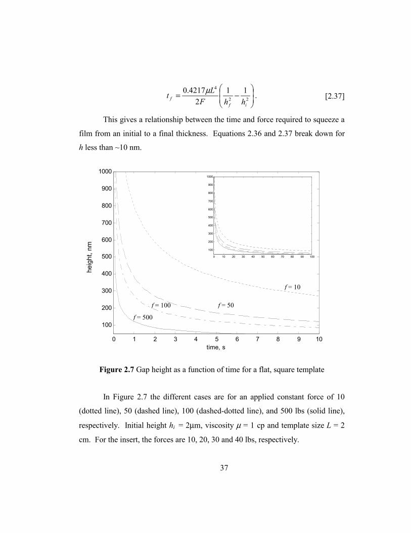
Lt µ . [2.37]

This gives a relationship between the time and force required to squeeze a

film from an initial to a final thickness. Equations 2.36 and 2.37 break down for

h less than ~10 nm.

0 1 2 3 4 5 6 7 8 9 10

100

200

300

400

500

600

700

800

900

1000

time, s

h, nm

Figure 2.7 Gap height as a function of time for a flat, square template

In Figure 2.7 the different cases are for an applied constant force of 10

(dotted line), 50 (dashed line), 100 (dashed-dotted line), and 500 lbs (solid line),

respectively. Initial height hi = 2µm, viscosity µ = 1 cp and template size L = 2

cm. For the insert, the forces are 10, 20, 30 and 40 lbs, respectively.

f = 10

f = 50 f = 100

f = 500

heig

ht, n

m

0 10 20 30 40 50 60 70 80 90 100

100

200

300

400

500

600

700

800

900

1000

38

For the case of 10 psi of pressure, over 75 seconds are required for the

film thickness to be reduced from 2 µm to 100 nm. The times to reach 100 nm

and 200 nm base layers are summarized in Table 2.1.

Applied Force (lbs) Time to 100 nm (s) Time to 200 nm (s)

10 75.6 18.8

20 37.8 9.4

30 25.2 6.2

40 18.9 4.7

50 15.1 3.7

100 7.5 1.9

500 1.5 0.37

Table 2.1 Time required to reach desired base layer thickness with constant force application for the case of a flat, square template.

Parameters used in equations 2.36 and 2.37 were hi = 2µm, µ = 1 cp and L = 2

cm.

2.4.2 3D Pressure Distribution for Parallel, Circular Plates

An analytic solution to the squeeze film pressure distribution for a finite

fluid drop centered between a flat, circular plate in parallel sinkage is considered.

Due to the rotational symmetry, an analytic solution is readily found. The

Reynolds equation in cylindrical coordinates and the derivation for the analytic

solutions to the pressure distribution and the force are given in Appendix A. The

pressure is a paraboloid of revolution of the form

39

( )hdt

dhh

rrp b γµ 233

22 −−= [2.38]

The force is obtained by integrating with respect to r and θ

−−=

hr

dtdh

hr

F bb2

3

4

43

2γµπ [2.39]

Equations 2.38 and 2.39 were used to perform numerical simulations of the

equation of motion where fluid is modeled with boundary conditions that evolve

as the fluid is squeezed out from between the surfaces. This is discussed in

Chapter 4.

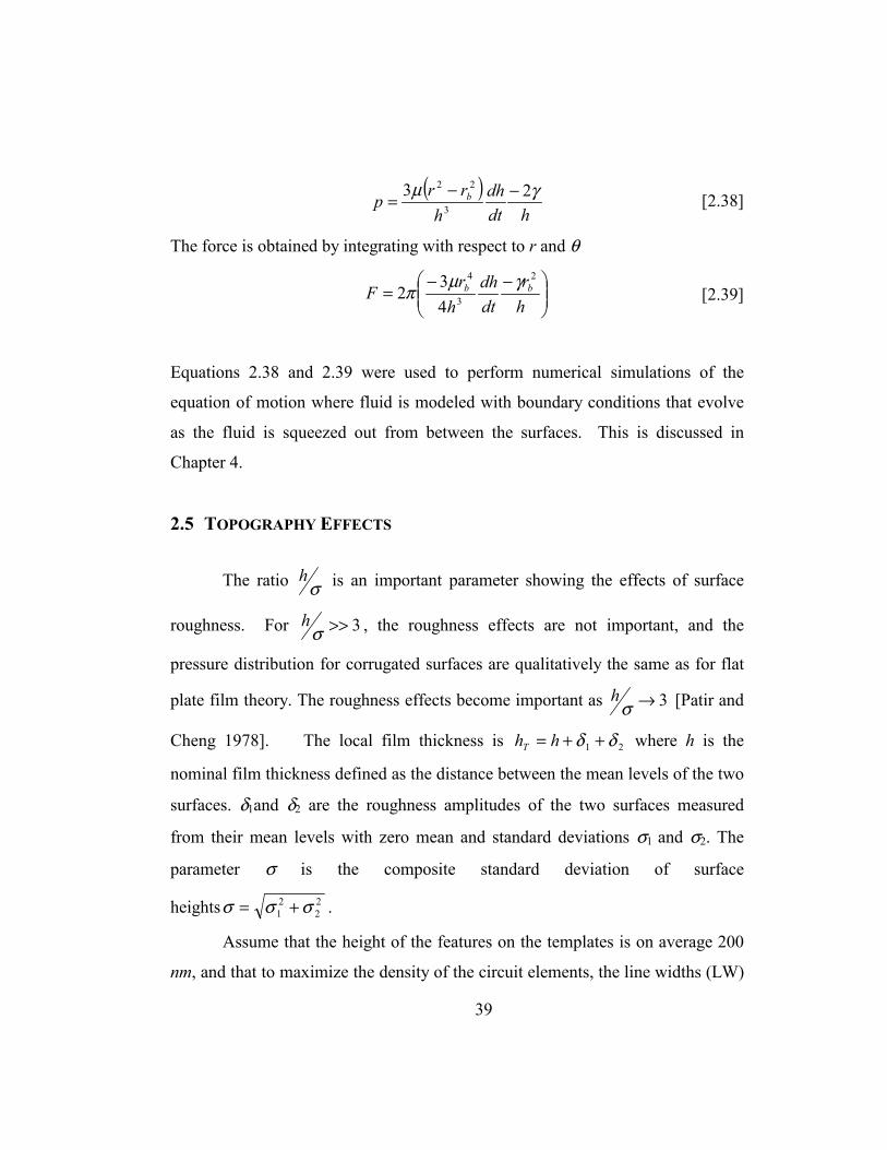
2.5 TOPOGRAPHY EFFECTS

The ratio σh is an important parameter showing the effects of surface

roughness. For 3>>σh , the roughness effects are not important, and the

pressure distribution for corrugated surfaces are qualitatively the same as for flat

plate film theory. The roughness effects become important as 3→σh [Patir and

Cheng 1978]. The local film thickness is 21 δδ ++= hhT where h is the

nominal film thickness defined as the distance between the mean levels of the two

surfaces. δ1and δ2 are the roughness amplitudes of the two surfaces measured

from their mean levels with zero mean and standard deviations σ1 and σ2. The

parameter σ is the composite standard deviation of surface

heights 22

21 σσσ += .

Assume that the height of the features on the templates is on average 200

nm, and that to maximize the density of the circuit elements, the line widths (LW)

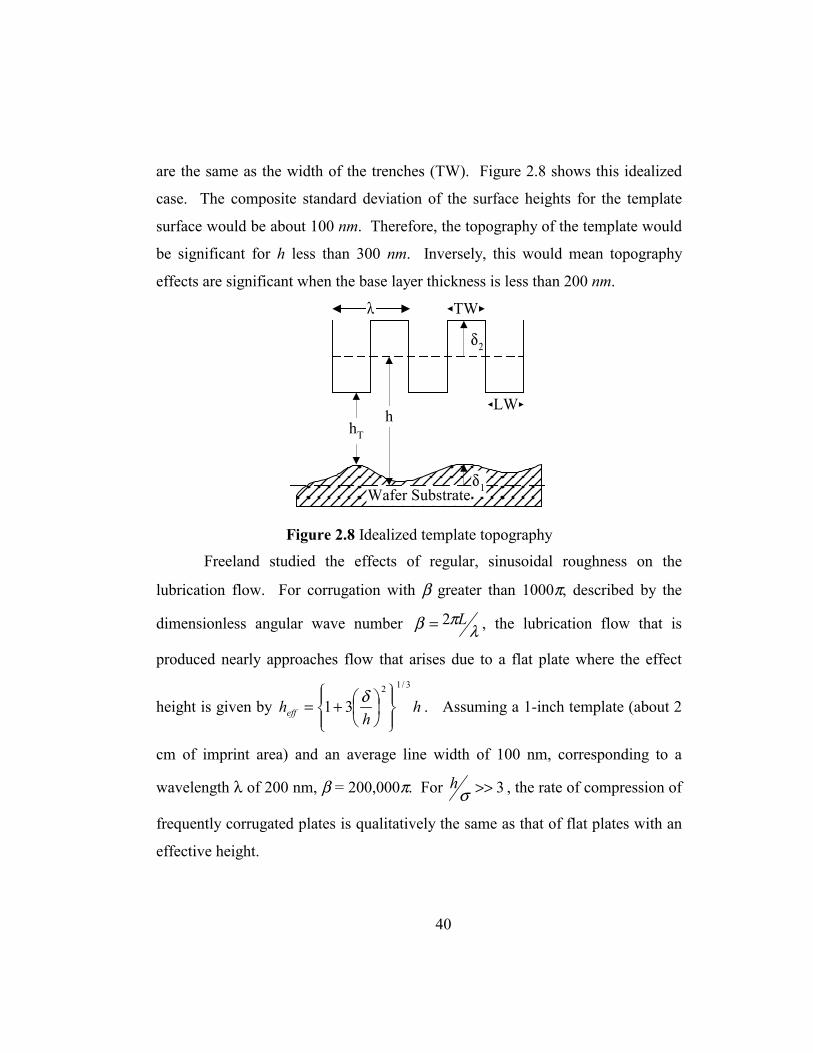
40

are the same as the width of the trenches (TW). Figure 2.8 shows this idealized

case. The composite standard deviation of the surface heights for the template

surface would be about 100 nm. Therefore, the topography of the template would

be significant for h less than 300 nm. Inversely, this would mean topography

effects are significant when the base layer thickness is less than 200 nm.

δ2

hT

LW

TWλ

Wafer Substrate

h

δ1

Figure 2.8 Idealized template topography

Freeland studied the effects of regular, sinusoidal roughness on the

lubrication flow. For corrugation with β greater than 1000π, described by the

dimensionless angular wave number λπβ L2= , the lubrication flow that is

produced nearly approaches flow that arises due to a flat plate where the effect

height is given by hh

heff

3/12

31

+= δ . Assuming a 1-inch template (about 2

cm of imprint area) and an average line width of 100 nm, corresponding to a

wavelength λ of 200 nm, β = 200,000π. For 3>>σh , the rate of compression of

frequently corrugated plates is qualitatively the same as that of flat plates with an

effective height.

41

Chapter 3: Active Stage Design

The practical development of the SFIL process requires that the base

layers are thin and uniform. An active stage machine is currently being designed

and implemented to allow scientific studies of the imprinting process. This

machine will have independent, high-resolution actuators and a feedback control

system to squeeze the etch barrier fluid prior to UV exposure. The requirements

and embodiment of such an active stage system are presented in this chapter.

3.1 OPTIMIZING BASE LAYER THICKNESS, ORIENTATION ALIGNMENT, AND THROUGHPUT

The ideal imprint process would lead to an etch barrier with a zero base layer

thickness. However, a zero base layer thickness cannot be obtained in finite time

with finite pressure. From the analysis in chapter 2, it can be seen that for a finite

pressure an infinite time is required to obtain a zero base layer thickness.

Experimental results from the multi-imprint machine support this theoretical

result in that base layers below 100 nm have been very difficult to achieve. In

reality, there is a tradeoff between throughput and base layer thickness since a

thinner base layer would require more time to achieve. If a base layer of uniform

thickness and of the order of the imprinted features (typically 200 nm) is

obtained, then a preliminary etching can eliminate the base layer without affecting

the fidelity of the imprinted features. Therefore, a base layer thickness in the

range of 100 to 200 nm would provide an optimal solution to both throughput

requirements and imprinted feature fidelity.

In the initial test beds for SFIL development, a coarse, micron-level pre-

calibration stage ensures that any initial orientation misalignment of the template

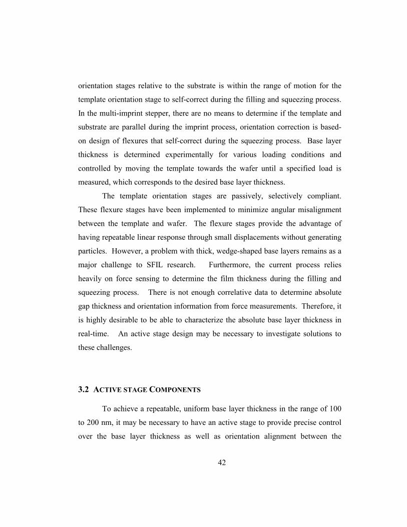
42

orientation stages relative to the substrate is within the range of motion for the

template orientation stage to self-correct during the filling and squeezing process.

In the multi-imprint stepper, there are no means to determine if the template and

substrate are parallel during the imprint process, orientation correction is based-

on design of flexures that self-correct during the squeezing process. Base layer

thickness is determined experimentally for various loading conditions and

controlled by moving the template towards the wafer until a specified load is

measured, which corresponds to the desired base layer thickness.

The template orientation stages are passively, selectively compliant.

These flexure stages have been implemented to minimize angular misalignment

between the template and wafer. The flexure stages provide the advantage of

having repeatable linear response through small displacements without generating

particles. However, a problem with thick, wedge-shaped base layers remains as a

major challenge to SFIL research. Furthermore, the current process relies

heavily on force sensing to determine the film thickness during the filling and

squeezing process. There is not enough correlative data to determine absolute

gap thickness and orientation information from force measurements. Therefore, it

is highly desirable to be able to characterize the absolute base layer thickness in

real-time. An active stage design may be necessary to investigate solutions to

these challenges.

3.2 ACTIVE STAGE COMPONENTS

To achieve a repeatable, uniform base layer thickness in the range of 100

to 200 nm, it may be necessary to have an active stage to provide precise control

over the base layer thickness as well as orientation alignment between the

43

template and the wafer. As a part of the research for this thesis, an active stage

test bed is being developed. The motion capability of the active stage system is

based on the ideal Revolute Prismatic Ball (RPB) stage. The RPB platform has

been thoroughly analyzed [Johnson 1999].

The systems that make up this test bed are 1) a wafer stage assembly, 2)

template orientation stages 3) a micro-fluidic etch barrier dispensing system, 4) a

high-resolution actuation system, 5) a gap sensing/orientation measurement

system, and 6) a force measurement system. Each system must be designed or

purchased as a modular component so that design modifications can be

implemented or customized within reasonable costs and time constraints. The

following discussion will provide some insight into the design requirements of the

subsystems relevant to this research. The details of the gap sensing theory and

implementation are given in chapter 4. A complete discussion of the entire active

stage project is beyond the scope of this thesis, as the active stage test bed is

currently in its infancy stage.

3.2.1 Wafer Stage Assembly

The wafer stage must bring the wafer substrate to within the motion range

of the DC Mike motor and hold the wafer in place during imprinting. The wafer

chuck must hold the wafer with minimal distortion by providing a uniform

pressure across the backside of the wafer. Current wafer manufacturers provide

wafers with low frequency height variations across their diameter. Using a flat

vacuum wafer chuck with uniform pressure across the supporting surface can

minimize these oscillations. Figure 3.1 shows the current embodiment of the

wafer stage assembly. Air solenoids lift the wafer to within the motion range of

the actuation system.

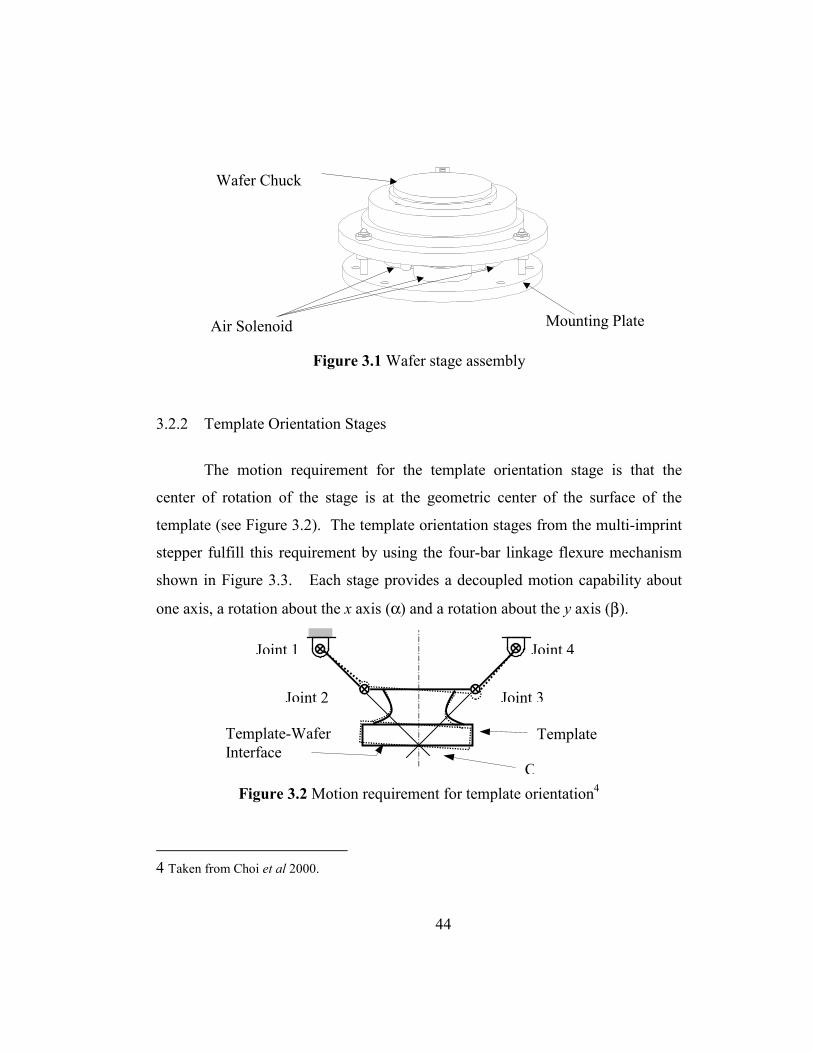
44

Figure 3.1 Wafer stage assembly

3.2.2 Template Orientation Stages

The motion requirement for the template orientation stage is that the

center of rotation of the stage is at the geometric center of the surface of the

template (see Figure 3.2). The template orientation stages from the multi-imprint

stepper fulfill this requirement by using the four-bar linkage flexure mechanism

shown in Figure 3.3. Each stage provides a decoupled motion capability about

one axis, a rotation about the x axis (α) and a rotation about the y axis (β).

Figure 3.2 Motion requirement for template orientation4

4 Taken from Choi et al 2000.

C

Joint 1

Joint 2

Template Template-Wafer Interface

Joint 3

Joint 4

Wafer Chuck

Mounting Plate Air Solenoid

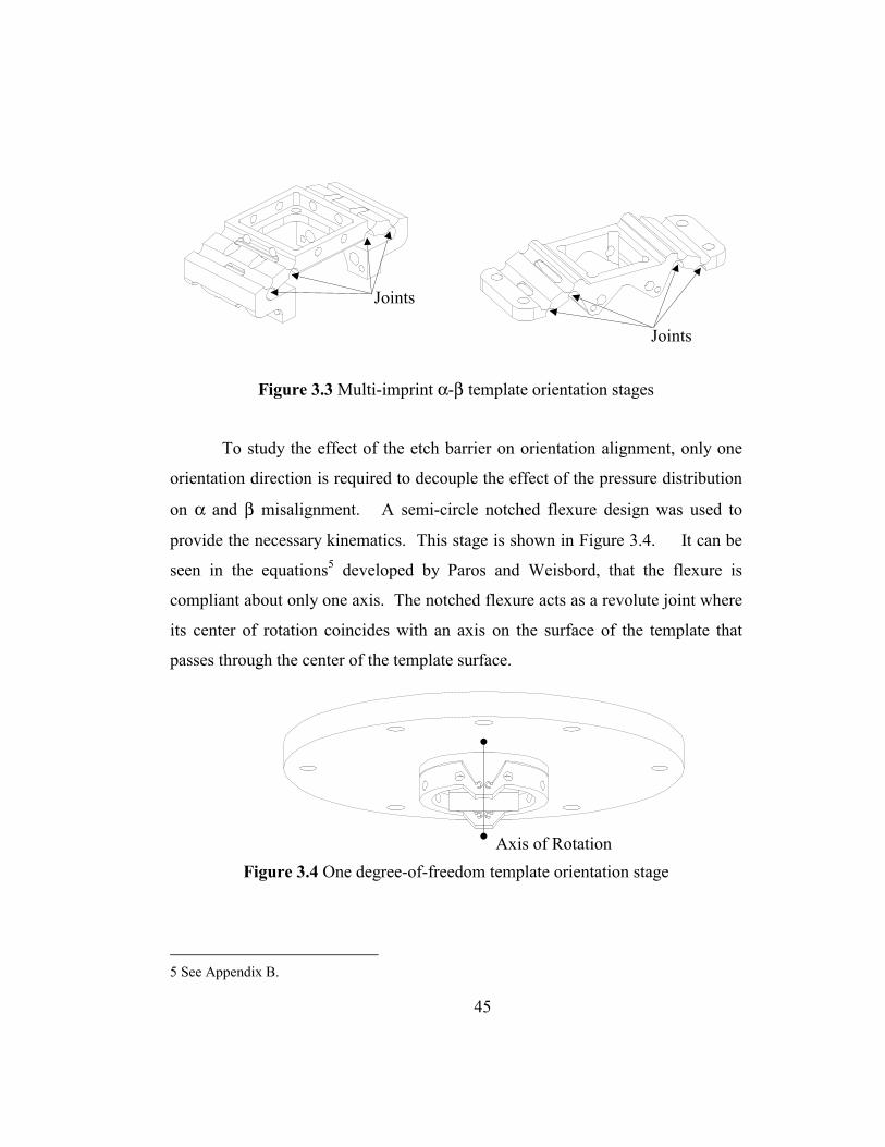
45

Figure 3.3 Multi-imprint α-β template orientation stages

To study the effect of the etch barrier on orientation alignment, only one

orientation direction is required to decouple the effect of the pressure distribution

on α and β misalignment. A semi-circle notched flexure design was used to

provide the necessary kinematics. This stage is shown in Figure 3.4. It can be

seen in the equations5 developed by Paros and Weisbord, that the flexure is

compliant about only one axis. The notched flexure acts as a revolute joint where

its center of rotation coincides with an axis on the surface of the template that

passes through the center of the template surface.

Figure 3.4 One degree-of-freedom template orientation stage

5 See Appendix B.

Axis of Rotation

Joints

Joints

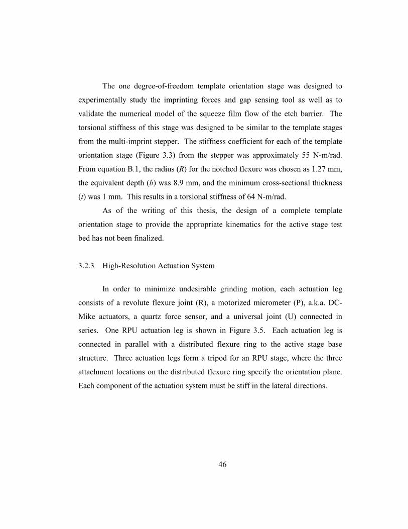
46

The one degree-of-freedom template orientation stage was designed to

experimentally study the imprinting forces and gap sensing tool as well as to

validate the numerical model of the squeeze film flow of the etch barrier. The

torsional stiffness of this stage was designed to be similar to the template stages

from the multi-imprint stepper. The stiffness coefficient for each of the template

orientation stage (Figure 3.3) from the stepper was approximately 55 N-m/rad.

From equation B.1, the radius (R) for the notched flexure was chosen as 1.27 mm,

the equivalent depth (b) was 8.9 mm, and the minimum cross-sectional thickness

(t) was 1 mm. This results in a torsional stiffness of 64 N-m/rad.

As of the writing of this thesis, the design of a complete template

orientation stage to provide the appropriate kinematics for the active stage test

bed has not been finalized.

3.2.3 High-Resolution Actuation System

In order to minimize undesirable grinding motion, each actuation leg

consists of a revolute flexure joint (R), a motorized micrometer (P), a.k.a. DC-

Mike actuators, a quartz force sensor, and a universal joint (U) connected in

series. One RPU actuation leg is shown in Figure 3.5. Each actuation leg is

connected in parallel with a distributed flexure ring to the active stage base

structure. Three actuation legs form a tripod for an RPU stage, where the three

attachment locations on the distributed flexure ring specify the orientation plane.

Each component of the actuation system must be stiff in the lateral directions.

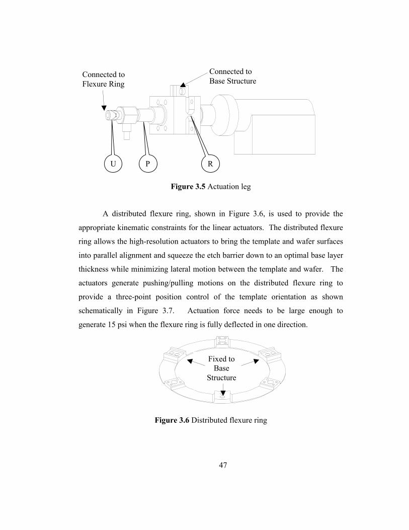
47

Figure 3.5 Actuation leg

A distributed flexure ring, shown in Figure 3.6, is used to provide the

appropriate kinematic constraints for the linear actuators. The distributed flexure

ring allows the high-resolution actuators to bring the template and wafer surfaces

into parallel alignment and squeeze the etch barrier down to an optimal base layer

thickness while minimizing lateral motion between the template and wafer. The

actuators generate pushing/pulling motions on the distributed flexure ring to

provide a three-point position control of the template orientation as shown

schematically in Figure 3.7. Actuation force needs to be large enough to

generate 15 psi when the flexure ring is fully deflected in one direction.

Figure 3.6 Distributed flexure ring

RP U

Connected to Base Structure

Connected to Flexure Ring

Fixed to Base

Structure

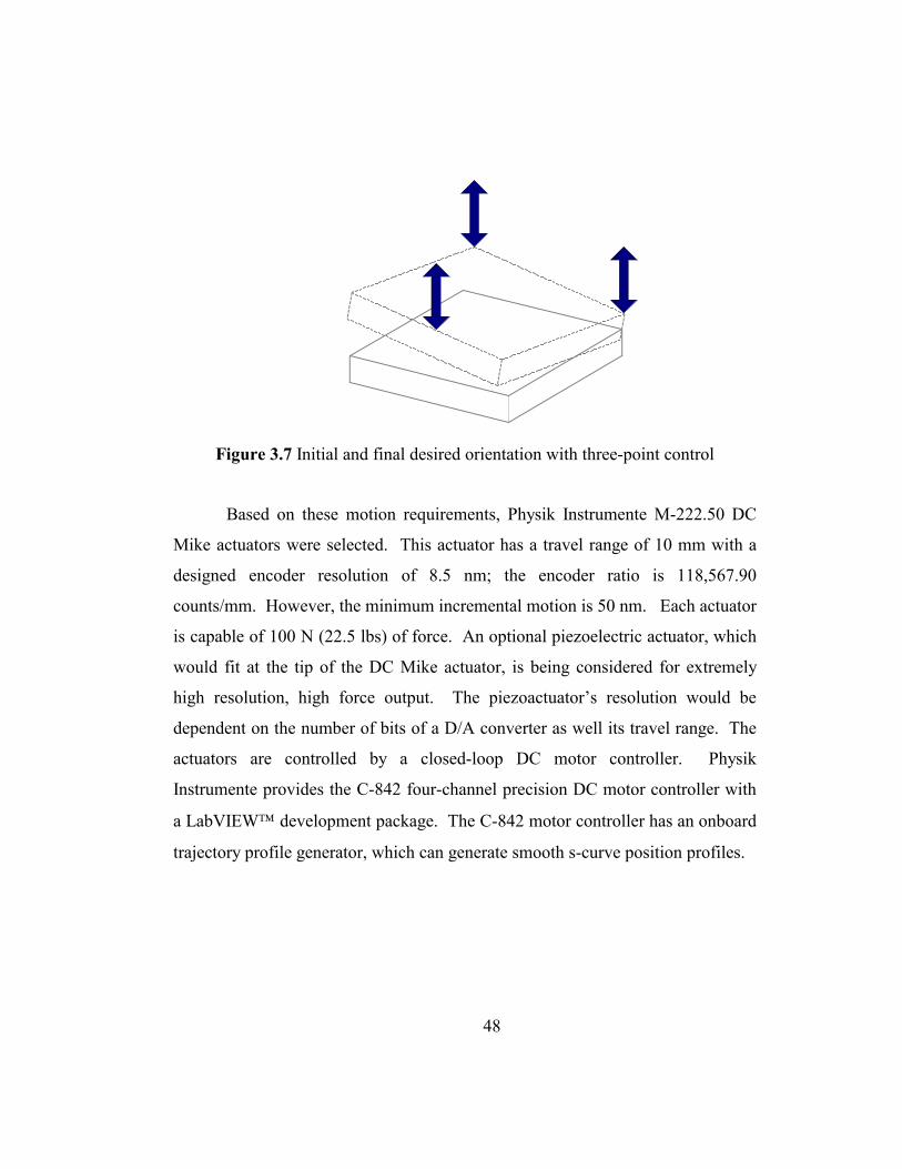
48

Figure 3.7 Initial and final desired orientation with three-point control

Based on these motion requirements, Physik Instrumente M-222.50 DC

Mike actuators were selected. This actuator has a travel range of 10 mm with a

designed encoder resolution of 8.5 nm; the encoder ratio is 118,567.90

counts/mm. However, the minimum incremental motion is 50 nm. Each actuator

is capable of 100 N (22.5 lbs) of force. An optional piezoelectric actuator, which

would fit at the tip of the DC Mike actuator, is being considered for extremely

high resolution, high force output. The piezoactuator’s resolution would be

dependent on the number of bits of a D/A converter as well its travel range. The

actuators are controlled by a closed-loop DC motor controller. Physik

Instrumente provides the C-842 four-channel precision DC motor controller with

a LabVIEW development package. The C-842 motor controller has an onboard

trajectory profile generator, which can generate smooth s-curve position profiles.

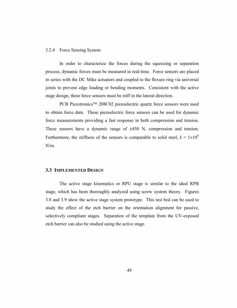
49

3.2.4 Force Sensing System

In order to characterize the forces during the squeezing or separation

process, dynamic forces must be measured in real-time. Force sensors are placed

in series with the DC Mike actuators and coupled to the flexure ring via universal

joints to prevent edge loading or bending moments. Consistent with the active

stage design, these force sensors must be stiff in the lateral direction.

PCB Piezotronics 208C02 piezoelectric quartz force sensors were used

to obtain force data. These piezoelectric force sensors can be used for dynamic

force measurements providing a fast response in both compression and tension.

These sensors have a dynamic range of ±450 N, compression and tension.

Furthermore, the stiffness of the sensors is comparable to solid steel, k = 1×109

N/m.

3.3 IMPLEMENTED DESIGN

The active stage kinematics or RPU stage is similar to the ideal RPB

stage, which has been thoroughly analyzed using screw system theory. Figures

3.8 and 3.9 show the active stage system prototype. This test bed can be used to

study the effect of the etch barrier on the orientation alignment for passive,

selectively compliant stages. Separation of the template from the UV-exposed

etch barrier can also be studied using the active stage.

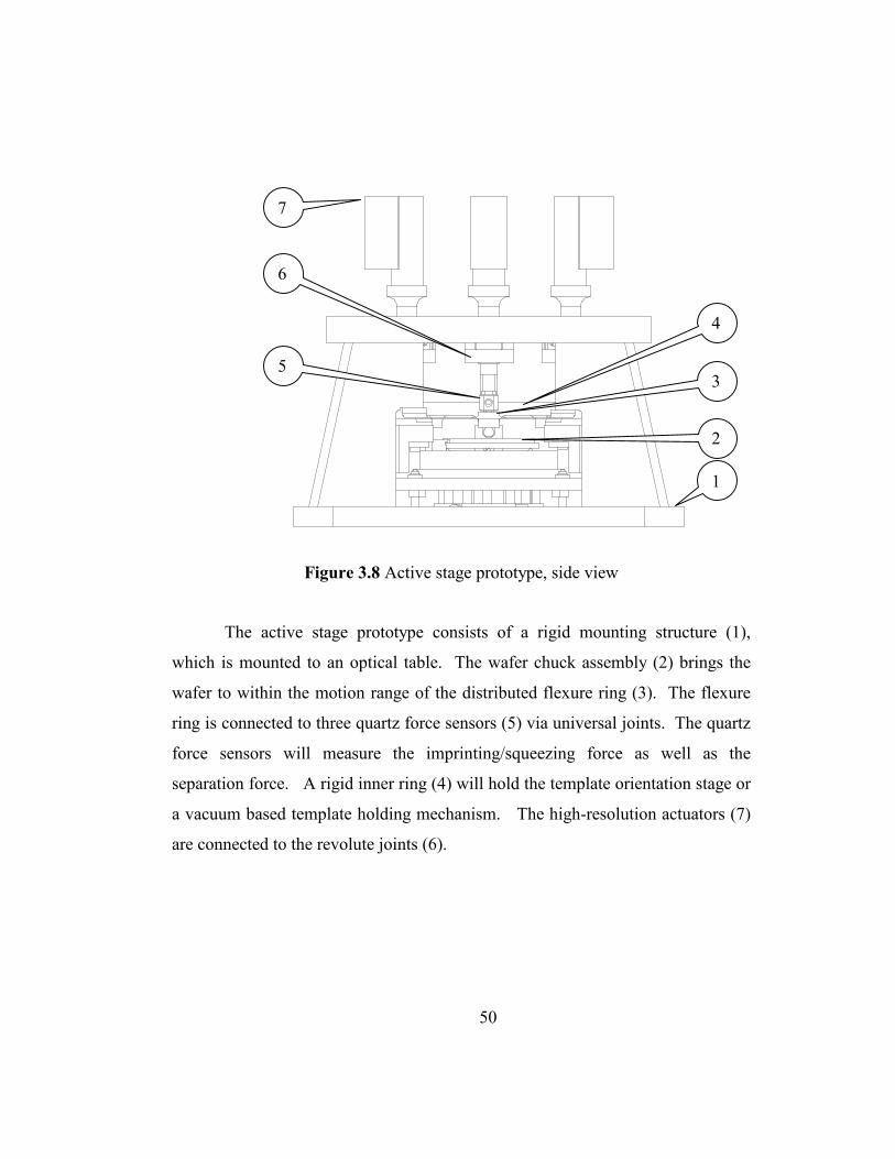
50

Figure 3.8 Active stage prototype, side view

The active stage prototype consists of a rigid mounting structure (1),

which is mounted to an optical table. The wafer chuck assembly (2) brings the

wafer to within the motion range of the distributed flexure ring (3). The flexure

ring is connected to three quartz force sensors (5) via universal joints. The quartz

force sensors will measure the imprinting/squeezing force as well as the

separation force. A rigid inner ring (4) will hold the template orientation stage or

a vacuum based template holding mechanism. The high-resolution actuators (7)

are connected to the revolute joints (6).

1

2

3

4

5

6

7

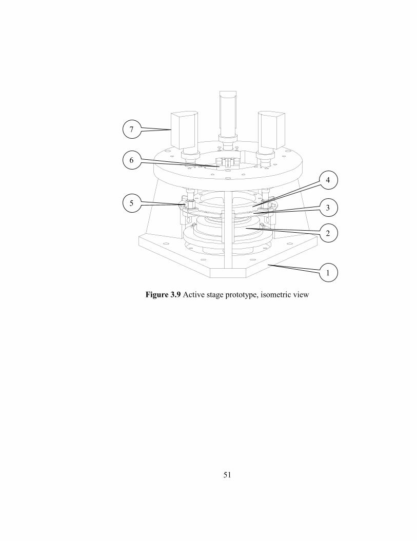
51

Figure 3.9 Active stage prototype, isometric view

1

2

3

4

5

6

7

52

Chapter 4: Real-Time Gap Sensing Via Fast Fourier Transforms of Spectral Reflectivity

As part of an active stage system, a feedback control system is required to

accurately align the template and the wafer substrate. Several techniques were

considered to obtain real-time gap information at several locations between the

template and wafer. Based on specific design requirements, FFT-based spectral

reflectometry is relatively low-cost method that promises to deliver real-time gap

sensing for SFIL.

4.1 INTRODUCTION

In the multi-imprint stepper, the template calibration stages can align the

template and wafer to within a single interference fringe across a one-inch

template. However, the initial orientation of the template may become

misaligned beyond the calibration specifications due to excessive forces, hard

contact with the wafer, etc. Correction requires that the template be removed and

the calibration to be repeated. A real-time gap sensing method implemented in

an active stage system will help to solve the issues of calibration, base layer

thickness, and wedged base layers. During the squeezing process, an in situ

spectral reflectometry technique based on Fast Fourier Transform (FFT) analysis

will provide the necessary gap and orientation information. Orientation

information is obtained in the form of gap information between two flats at three

points.

Other optical methods to measure film thickness have been proposed

which employ spectral or Fourier analysis of the reflectivity data from thin films.

[Bouldin et al 2000], [Chalmers 2001], [Chason 2000], and [Sakurai and Iida

1992]. However, these methods are either not commercially available or not

53

directly applicable to in situ gap sensing in SFIL. Some of these methods require

precise angular sweeps such as the X-ray method described by Sakurai and Iida.

Others can be quite computationally complex, requiring comparisons between

experimental and theoretical waveforms, which are stored in a database for a

particular film with known optical properties such as the index of refraction. This

search for matching waveforms can be time-consuming. In this research, a real-

time gap sensing method that can potentially measure thin films down to 50 nm

has been applied to measure the gap between the template and the substrate

during the squeezing process. This chapter attempts to provide the background in

the optical theory necessary to understand the basis for this innovative tool.

4.2 ANALYSIS OF SPECTRAL REFLECTIVITY

When an optical flat is placed in near contact with another optically flat

surface, dark and bright bands will be formed. These bands are known as

interference fringes, caused by constructive (bright bands) and destructive

interference (dark bands) of light, and their shape gives a visual representation of

the flatness and parallelism of the surface being tested. The parallelism and

thickness of the gap is indicated by the amount of curvature and spacing between

the interference fringes. Straight, parallel, and evenly spaced interference fringes

indicate that the two flat surfaces are parallel along one axis. Spectral

reflectometry relies on this constructive-destructive interference property of light.

For optically thin films in the visible wavelength range, the oscillations in

the reflectivity are periodic in wavenumber (k = 2π/λ) such as shown the by the

equation for the reflectivity of a single optical thin film

54

( ) ( )

( ) ( )λπρρρρλπρρρρ

λαα

αα

/4cos21/4cos2

3,22,122

3,22,1

3,22,122

3,22

2,1

ndeendee

Rdd

dd

−−

−−

+−−+

= [4.1]

where 1, +iiρ are the reflectivity coefficients at the interface of the

ii and 1− interface, n index of refraction, d is the thickness of the film, and α is

the absorption coefficient of the film. Generally speaking, the index of refraction

n varies with wavelength λ.

Equation 4.1 was derived by assuming that the substrate exhibits perfect

reflection and no absorption. It can be shown that equation 4.1 can be reduced to

the general form

( ) ( )kndBAR 2cos+=λ [4.2]

To better understand equation 4.2, take a simple optical thin film

composed of the template, air, and the substrate. Since the template is very thick,

the light passing through it does not see the effect of the template. Figure 4.1

illustrates this example with a thin film of air above the substrate. Incident light,

with energy EI, is reflected off the template-gap interface with energy ER0 and

partially transmitted into the gap and this is in turn reflected off the substrate.

The light reflected from the substrate is then partially reflected off and transmitted

through the interface through the template. When the light ER0 and ER1 are in

phase, they will add constructively. When the light ER0 and ER1 are out of phase

by they will add destructively.

55

Figure 4.1 Interference effect

Gap sensing is based on the periodicity of the reflectivity spectrum, as

seen in equation 4.2. Since the spectral reflectivity is periodic in wavenumber,

for 400 ~ 800 nm. Fourier analysis can be used to perform a spectral

decomposition. The calculation of the thickness of an optical thin film is trivial

once this information is obtained. The thickness of a film can be computed as

nwn

FFT

wnMagid∆

=2

[4.3]

where iFFT is the index of the FFT maximum and nwn is the wavenumber averaged

index of refraction. The ratio of sampled points in the wavenumber spectrum

taken at even intervals over a spectral range, maxmin

11λλ−=∆ nw , to the number of

points in the FFT is defined as the magnification factor, Mag [Colburn 2001].

This method can measure film thickness down to about 350 nm based on a

wavenumber averaged refractive index of 1.5 and has been demonstrated to be in

good agreement with spectral ellipsometry and profilometry. For films below 350

nm, Inflection-Maximum-Minimum Analysis (IMMA) is used to compute the

film thickness. The reader is referred to Chapter 8 of Colburn’s dissertation for

more detailed information the theoretical background of FFT-based spectral

reflectometry. This gap sensing system is under development for Dissolution

EI

Substrate

Air Film

ER0 ER1

dFilm with Refractive Index n

λ

56

Rate Monitoring and is adapted for measuring film thickness during the squeeze

film experiments.

Equation 4.2 is demonstrated for a simulated film with a thickness of 500

nm. In Figure 4.2, the theoretical reflectivity is plotted as a function of

wavelength. The plot resembles an expanding sine wave. However, when the

reflectivity is plotted as a function of wavenumber in Figure 4.3, it is clearly seen

that this is a periodic signal.

300 400 500 600 700 800 900 1000 1100-1

-0.8

-0.6

-0.4

-0.2

0

0.2

0.4

0.6

0.8

1

wavelength, nm

Figure 4.2 Normalized intensity of a 500 nm film as a function of wavelength

refle

ctiv

ity

57

0.005 0.01 0.015 0.02-1

-0.8

-0.6

-0.4

-0.2

0

0.2

0.4

0.6

0.8

1

wavenumber, 1/nm

Figure 4.3 Normalized intensity of a 500 nm film as a function of wavenumber

The Power Spectral Density (PSD) is computed for the corresponding

signal and plotted as a function of the thickness, which is proportional to the

index of the Fourier transform and is given by equation 4.3. From Figure 4.4, it

can be seen that the peak at 500 nm corresponds to the thickness of the film.

The resolution of the algorithm is given by

nwnMagresolution∆

=2

[4.4]

The size of the FFT improves the resolution, while it increases the processing

time. Further, the spectral range of the data also affects the resolution. In the

visible range, 400 – 800 nm, with an index of refraction of 1.5 and taking 128 (27)

sample points of data and performing a 16384-point FFT (214), results in a

resolution of 2 nm. This theoretical work was the proving ground for the

embodiment used in the experiments. The implementation details are further

discussed in chapter 6. This includes accounts of the hardware used, signal

processing issues, and areas for improvement.

refle

ctiv

ity

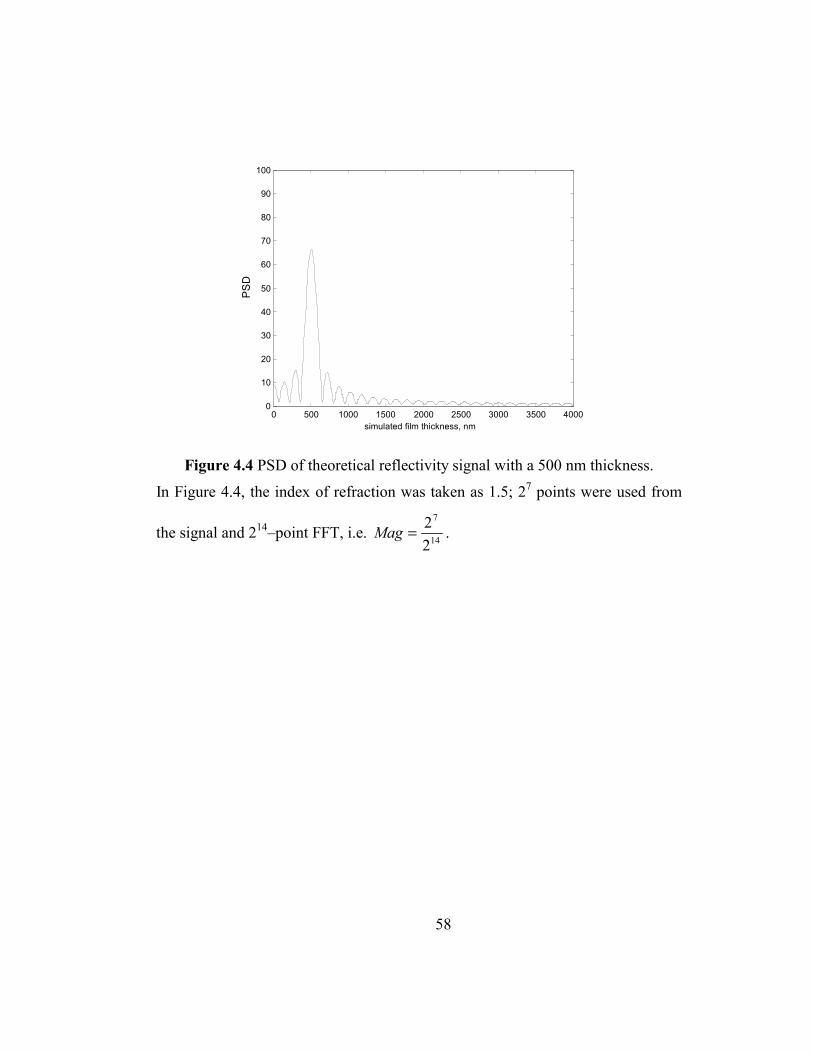
58

0 500 1000 1500 2000 2500 3000 3500 4000 0

10

20

30

40

50

60

70

80

90

100

simulated film thickness, nm

Figure 4.4 PSD of theoretical reflectivity signal with a 500 nm thickness.

In Figure 4.4, the index of refraction was taken as 1.5; 27 points were used from

the signal and 214–point FFT, i.e. 14

7

22=Mag .

PSD

59

Chapter 5: Numerical Simulations

A series of numerical simulations to predict the performance of the

imprinting systems used in SFIL are discussed in this chapter. A model of the

mechanical system was developed, which considered two primary modes of

compliance - axial and torsional. Initial conditions were selected to be similar to

those in the actual SFIL experiments. The actuation was assumed to have an

ideal feedforward controller. The equations of motion were simulated using a

fourth order accurate Runge-Kutta scheme with adaptive time marching.

Simulation results are presented in this chapter for the case of an inclined surface

of infinite width with both single and double s-curve position control. Finally, the

case of a parallel, circular plate with a single fluid drop was simulated.

5.1 DYNAMIC SYSTEM MODEL

In this section the equations governing the dynamic response of the

imprinting system are presented. The dynamic equations are developed

assuming an imprinting system where the motion is governed by compliance in

two directions: the axial direction along the motion axis of the actuators and a

rotational direction about an orthogonal axis. The template holding mechanism

based on semi-circle notched flexures discussed in chapter 3 (see Figure 3.4) was

designed to be consistent with this assumption and is implemented in the active

stage test bed. Equivalently, a single rotational axis can be the orientation axis of

the template in the multi-imprint stepper where the axis of rotation is an axis that

is a linear combination of the motion provided by the α-β stages. This axis also

passes through the center of the template surface (see Figure 3.2). Henceforth

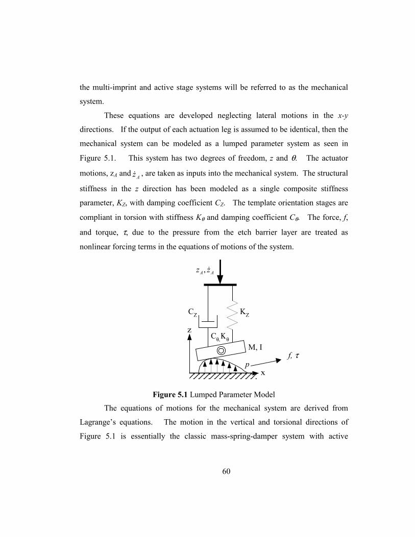
60

the multi-imprint and active stage systems will be referred to as the mechanical

system.

These equations are developed neglecting lateral motions in the x-y

directions. If the output of each actuation leg is assumed to be identical, then the

mechanical system can be modeled as a lumped parameter system as seen in

Figure 5.1. This system has two degrees of freedom, z and θ. The actuator

motions, zA and Az� , are taken as inputs into the mechanical system. The structural

stiffness in the z direction has been modeled as a single composite stiffness

parameter, KZ, with damping coefficient CZ. The template orientation stages are

compliant in torsion with stiffness Kθ and damping coefficient Cθ. The force, f,

and torque, τ, due to the pressure from the etch barrier layer are treated as

nonlinear forcing terms in the equations of motions of the system.

KZ

AA zz D,

M, ICθ,Κθ

CZ

px

z

Figure 5.1 Lumped Parameter Model

The equations of motions for the mechanical system are derived from

Lagrange’s equations. The motion in the vertical and torsional directions of

Figure 5.1 is essentially the classic mass-spring-damper system with active

f, τ

61

damping from the etch barrier. The dynamic behavior of such systems can be

described by

( ) ( ) ( )θθ DDDDDD ,,, zzfzzKzzCzM AZAZ =−+−+ [5.1]

and

( ) ( )θθτθθθθ θθDDDDD ,,,0 zzKCI =−++ [5.2]

where the fluid force and torque are functions of position and orientation. The

fluid couples the two, otherwise independent, motions. In the following sections,

the set of model parameters are presented with details on the selection of initial

conditions for the simulation.

5.2 SYSTEM PARAMETERS FOR NUMERICAL SIMULATION

5.2.1 Etch Barrier Fluid Properties

The capillary pressure is obtained using the surface tension coefficient for

the etch barrier formulation. The surface tension of the various etch barrier

formulations, which is composed of free radical generators and cross-linking

agents dissolved in a solution of organic monomer, silylated monomer, and

dimethyl siloxane oligomer derivatives, are all nearly identical to within

experimental error at 28 dynes/cm [Colburn et al 1999]. If the fluid between the

plates is water instead of etch barrier, the surface tension is 72 dynes/cm at 20°C.

From this, the boundary conditions due to the capillary pressure for the fluid

volume can be computed. The viscosity of the etch barrier layer is the same as

that of water at room temperature and atmospheric pressure, which is about 1 cP

(1 × 10-3 N⋅s/m2). Both the etch barrier and water were considered to have a

constant viscosity and to be incompressible.

62

5.2.2 Composite Stiffness and Damping Coefficients

The composite vertical stiffness, KZ, of the mechanical system was

computed from a distributed spring system as shown in Figure 5.2. The vertical

and torsional stiffness of flexure components with torsional compliance were

computed using equations from Paros and Weisbord. The relevant Paros and

Weisbord equations used to compute the stiffness for the components with

notched flexure joints are presented in Appendix B. These components include

the revolute joint (KRJ), the universal joint (KUJ), and the template holder (KTH).

KRF

M

KRJ

KDC

KUJ

KFS

KTH

Figure 5.2 Stiffness in the z direction of the active stage system

The stiffness of the actuator was approximated by assuming an aluminum

tube of 50 mm in length with a 5 mm inner radius and 6 mm outer radius. The

equation for the stiffness is then

L

EAk = [5.3]

where E is Young’s modulus for aluminum, A is the area seen by a vertical force

and L is the actuator length as shown in Figure 5.3. The length is an approximate

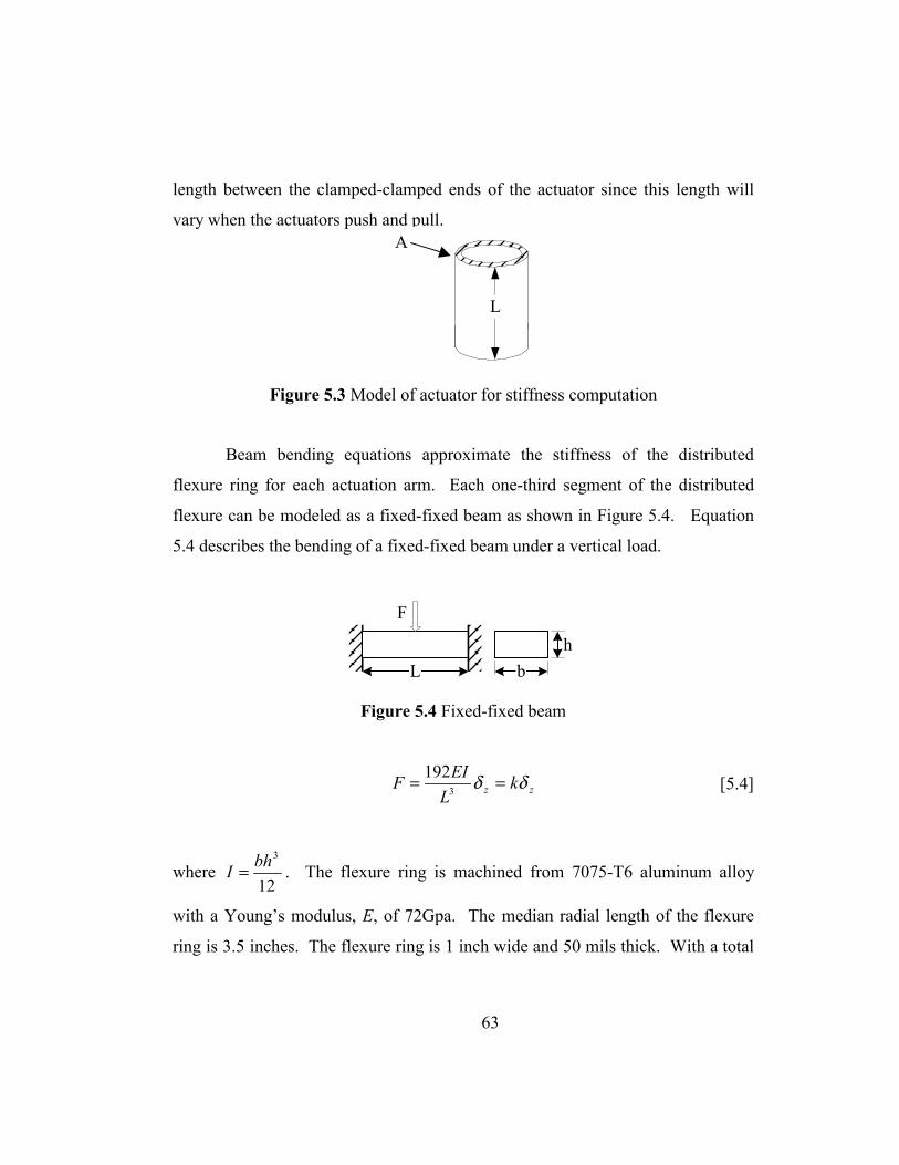
63

length between the clamped-clamped ends of the actuator since this length will

vary when the actuators push and pull.

L

Figure 5.3 Model of actuator for stiffness computation

Beam bending equations approximate the stiffness of the distributed

flexure ring for each actuation arm. Each one-third segment of the distributed

flexure can be modeled as a fixed-fixed beam as shown in Figure 5.4. Equation

5.4 describes the bending of a fixed-fixed beam under a vertical load.

F

L bh

Figure 5.4 Fixed-fixed beam

zz k

LEIF δδ == 3

192 [5.4]

where 12

3bhI = . The flexure ring is machined from 7075-T6 aluminum alloy

with a Young’s modulus, E, of 72Gpa. The median radial length of the flexure

ring is 3.5 inches. The flexure ring is 1 inch wide and 50 mils thick. With a total

A

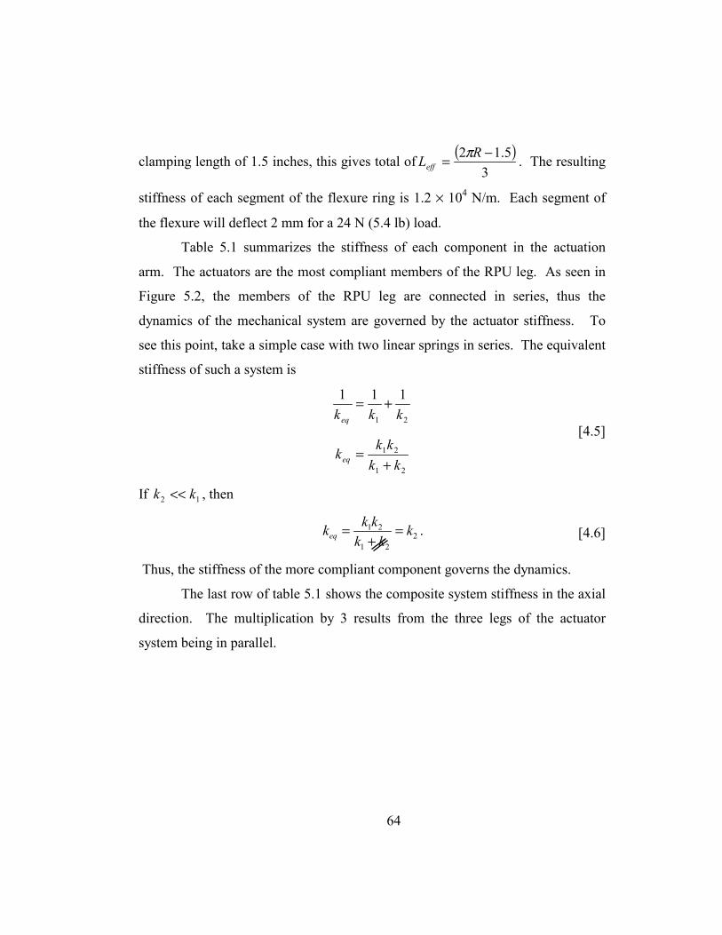
64

clamping length of 1.5 inches, this gives total of ( )3

5.12 −= RLeffπ . The resulting

stiffness of each segment of the flexure ring is 1.2 × 104 N/m. Each segment of

the flexure will deflect 2 mm for a 24 N (5.4 lb) load.

Table 5.1 summarizes the stiffness of each component in the actuation

arm. The actuators are the most compliant members of the RPU leg. As seen in

Figure 5.2, the members of the RPU leg are connected in series, thus the

dynamics of the mechanical system are governed by the actuator stiffness. To

see this point, take a simple case with two linear springs in series. The equivalent

stiffness of such a system is

21

111kkkeq

+=

21

21

kkkkkeq +

= [4.5]

If 12 kk << , then

2

21

21 kkk

kkkeq =+

= . [4.6]

Thus, the stiffness of the more compliant component governs the dynamics.

The last row of table 5.1 shows the composite system stiffness in the axial

direction. The multiplication by 3 results from the three legs of the actuator

system being in parallel.

65

Component Symbol Z-Stiffness

Revolute Joint KRJ 4.1 × 109

DC Mike Actuator KDC 5.0 × 107

Quartz Force Sensor KFS 1.0 × 109

Universal Joint KUJ 4.7 × 109

Template Holder KTH 7.2 × 108

Distributed Flexure Ring KRF 1.2 × 104

Composite System Stiffness KZ 4.4 × 107 × 3

Table 5.1 Mechanical system stiffness values

The equivalent inertial terms, M and I, were computed from

Pro/ENGINEER® solid models. The equivalent mass is approximately 1.5 kg.

The equivalent inertia is approximately 5 × 10-6 kg⋅m2. It is assumed that the

damping factor, ζ, for the mechanical system is 0.05. This gives the damping

coefficients as eqeqeq MKC ζ2= , thus CZ = 1400 N⋅s/m and Cθ = 2 × 10-3

N⋅m⋅s.

5.2.3 Model of Actuation System

The actuator motion is taken as input into the mechanical system and

assumed to have an ideal control scheme. The actuators are controlled by a PID

controller, which comes on board the Physik Instrument C-842 motor controller.

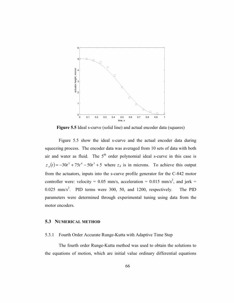
66

0 0.1 0.2 0.3 0.4 0.5 0.6 0.7 0.8 0.9 1 0

1

2

3

4

5

6

time, s

actu

ator

hei

ght,

mic

ron

Figure 5.5 Ideal s-curve (solid line) and actual encoder data (squares)

Figure 5.5 show the ideal s-curve and the actual encoder data during

squeezing process. The encoder data was averaged from 10 sets of data with both

air and water as fluid. The 5th order polynomial ideal s-curve in this case is

( ) 5507530 345 +−+−= ttttz A where zA is in microns. To achieve this output

from the actuators, inputs into the s-curve profile generator for the C-842 motor

controller were: velocity = 0.05 mm/s, acceleration = 0.015 mm/s2, and jerk =

0.025 mm/s2. PID terms were 300, 50, and 1200, respectively. The PID

parameters were determined through experimental tuning using data from the

motor encoders.

5.3 NUMERICAL METHOD

5.3.1 Fourth Order Accurate Runge-Kutta with Adaptive Time Step

The fourth order Runge-Kutta method was used to obtain the solutions to

the equations of motion, which are initial value ordinary differential equations

67

(ODE). With any numerical simulation both accuracy and stability of the method

in computing the solutions to the dynamics equations are important

considerations. The fourth order Runge-Kutta scheme has an increased region of

stability as compared with other explicit schemes such as second order Runge-

Kutta and explicit Euler. The stability diagram for the fourth order Runge-Kutta

scheme includes eigenvalues on the imaginary axis with a small portion involving

both positive real eigenvalues when the imaginary component is nonzero, i.e.

irc iλλλ += where when 0,0 >≠ ri λλ [Collis 2000].

The problem is conditionally stable. Since the initial gap is small, the

time step must be chosen carefully to maintain numerical stability. Numerical

instability exists in the analytical solution to the fluid damping force and damping

torque. Firstly, the film thickness cannot be less than zero. This would result in

the breakdown of the Reynolds equation. The pressure becomes infinite at zero

film thickness. Furthermore, hard contact between the template and wafer cannot

be modeled by the Reynolds equation. Secondly, the damping force and torque

are dependent on the state variables, ( )θθ DD ,,, zzf and ( )θθτ DD ,,, zz . Thus the

solution could become unstable since the eigenvalues of the system change during

the simulation. This phenomenon is observed during the simulations. For

example, an initial time step of 1 × 10-7 seconds or 0.1 microseconds will result in

a stable solution for the first part of the simulation when the base layer thickness

is large. Then this time step must be decreased for the solution to remain stable.

When the base layer thickness is below 500 nm, a time step of 1 nanosecond is

required to maintain numerical stability. With a very small time step such as 1

nanosecond, a 1 second simulation could easily extend over 24 hours in a C++

implementation on an 850 MHz computer with 128 MB of RAM and 256KB of

level 2 cache memory (L2 cache operations are faster than RAM). An adaptive

68

time marching is required to minimize computational time and provide accurate

solutions. This adaptation was done manually by providing the largest stable time

step as input into the simulation. These time steps were determined by brute

force. Each simulation was broken into several simulation time intervals. Then

the time step was decreased by a factor of 10 when the simulation showed signs

of instability. This was repeated until each run of the simulation was complete.

5.3.2 Modeling the Initial Conditions for an Imprint

The equations of motion for the mechanical system represent an initial

value problem. This ODE system requires a set of known initial conditions.

The set of initial conditions was chosen to reflect those existing in the imprinting

process. A further requirement was that these could be replicated in the

experimental setup.

The initial gap between the template and the wafer was assumed to be 2

µm. The initial conditions at the left and right boundaries of the flow at x = xα

and x = xβ are determined by simple volumetric calculations. For a template of

one square inch and a base layer thickness of 200 nm to completely fill the gap,

this requires that the volume of fluid dispensed is 0.13 µL (1.3 × 10-10 m3). This

minimizes material wastage as well as the force required to squeeze out the fluid.

The placement of this fluid volume is assumed to be a line of 2 mm width, which

completely wets the template along its length and is along the centerline of the

template surface. A 2 µm column of fluid 2.54 cm (1 inch) long and 2mm wide

is about 0.1 µL. This fluid volume would thus fill the gap at a base layer

thickness of between 100 and 200 nm.

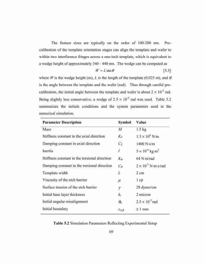
69

The feature sizes are typically on the order of 100-200 nm. Pre-

calibration of the template orientation stages can align the template and wafer to

within two interference fringes across a one-inch template, which is equivalent to

a wedge height of approximately 340 - 440 nm. The wedge can be computed as

θtanLW = [5.5]

where W is the wedge height (m), L is the length of the template (0.025 m), and θ

is the angle between the template and the wafer (rad). Thus through careful pre-

calibration, the initial angle between the template and wafer is about 2 × 10-5 rad.

Being slightly less conservative, a wedge of 2.5 × 10-5 rad was used. Table 5.2

summarizes the initials conditions and the system parameters used in the

numerical simulation.

Parameter Description Symbol Value

Mass M 1.5 kg

Stiffness constant in the axial direction KZ 1.3 × 108 N/m

Damping constant in axial direction CZ 1400 N⋅s/m

Inertia I 5 × 10-6 kg⋅m2

Stiffness constant in the torsional direction Kθ 64 N⋅m/rad

Damping constant in the torsional direction Cθ 2 × 10-3 N⋅m⋅s/rad

Template width L 2 cm

Viscosity of the etch barrier µ 1 cp

Surface tension of the etch barrier γ 28 dynes/cm

Initial base layer thickness hi 2 micron

Initial angular misalignment θ0 2.5 × 10-5 rad

Initial boundary xα,β ± 1 mm

Table 5.2 Simulation Parameters Reflecting Experimental Setup

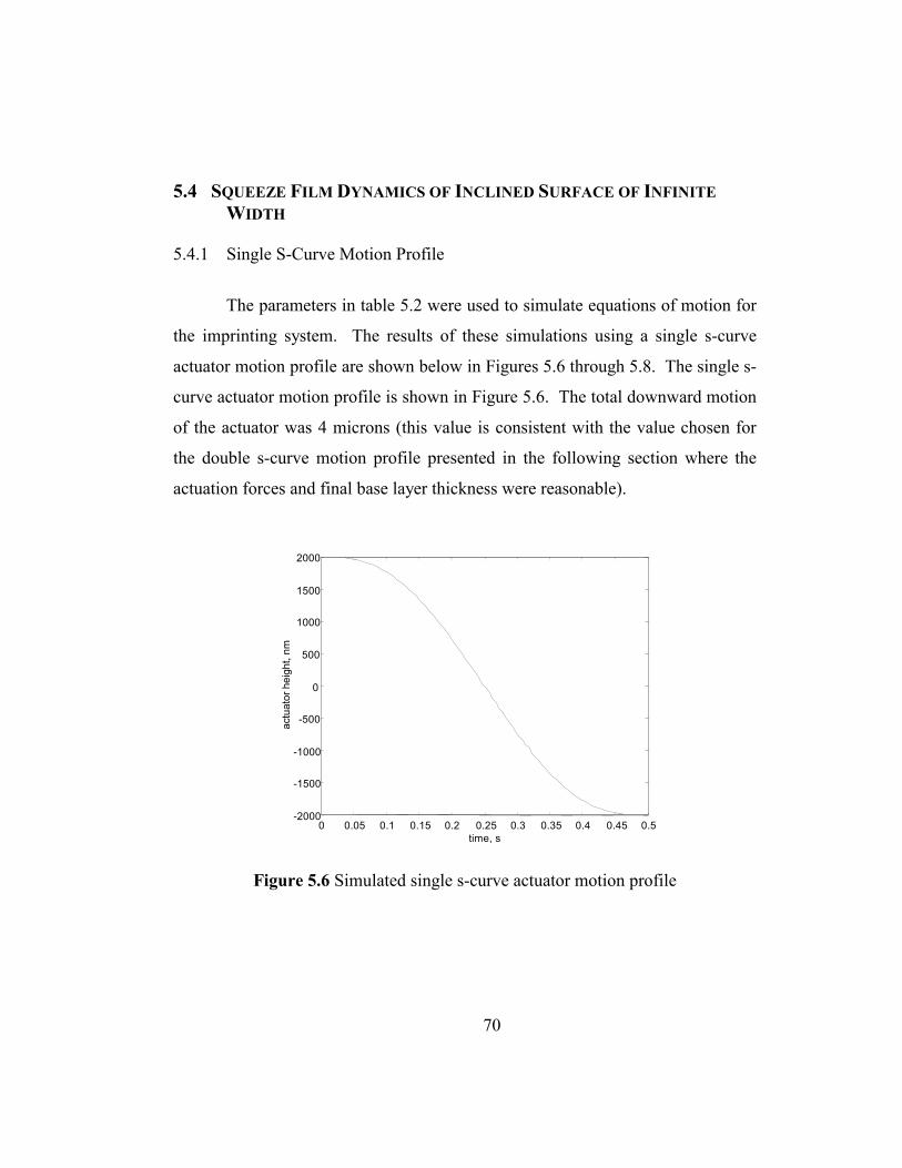
70

5.4 SQUEEZE FILM DYNAMICS OF INCLINED SURFACE OF INFINITE WIDTH

5.4.1 Single S-Curve Motion Profile

The parameters in table 5.2 were used to simulate equations of motion for

the imprinting system. The results of these simulations using a single s-curve

actuator motion profile are shown below in Figures 5.6 through 5.8. The single s-

curve actuator motion profile is shown in Figure 5.6. The total downward motion

of the actuator was 4 microns (this value is consistent with the value chosen for

the double s-curve motion profile presented in the following section where the

actuation forces and final base layer thickness were reasonable).

0 0.05 0.1 0.15 0.2 0.25 0.3 0.35 0.4 0.45 0.5 -2000

-1500

-1000

-500

0

500

1000

1500

2000

time, s

actu

ator

hei

ght,

nm

Figure 5.6 Simulated single s-curve actuator motion profile

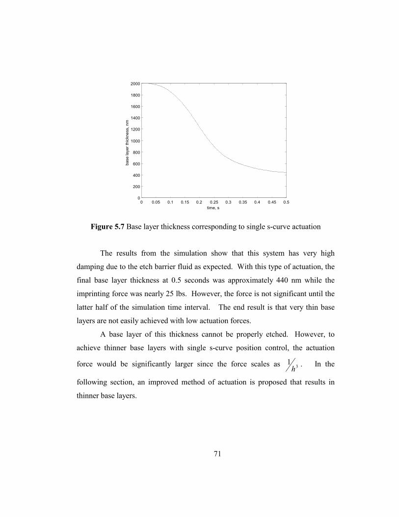
71

0 0.05 0.1 0.15 0.2 0.25 0.3 0.35 0.4 0.45 0.5 0 200 400 600 800

1000 1200 1400 1600 1800 2000

time, s

base

laye

r thi

ckne

ss, n

m

Figure 5.7 Base layer thickness corresponding to single s-curve actuation

The results from the simulation show that this system has very high

damping due to the etch barrier fluid as expected. With this type of actuation, the

final base layer thickness at 0.5 seconds was approximately 440 nm while the

imprinting force was nearly 25 lbs. However, the force is not significant until the

latter half of the simulation time interval. The end result is that very thin base

layers are not easily achieved with low actuation forces.

A base layer of this thickness cannot be properly etched. However, to

achieve thinner base layers with single s-curve position control, the actuation

force would be significantly larger since the force scales as 31

h . In the

following section, an improved method of actuation is proposed that results in

thinner base layers.

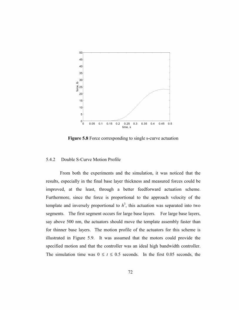
72

0 0.05 0.1 0.15 0.2 0.25 0.3 0.35 0.4 0.45 0.5 0 5

10 15 20 25 30 35 40 45 50

time, s

forc

e, lb

Figure 5.8 Force corresponding to single s-curve actuation

5.4.2 Double S-Curve Motion Profile

From both the experiments and the simulation, it was noticed that the

results, especially in the final base layer thickness and measured forces could be

improved, at the least, through a better feedforward actuation scheme.

Furthermore, since the force is proportional to the approach velocity of the

template and inversely proportional to h3, this actuation was separated into two

segments. The first segment occurs for large base layers. For large base layers,

say above 500 nm, the actuators should move the template assembly faster than

for thinner base layers. The motion profile of the actuators for this scheme is

illustrated in Figure 5.9. It was assumed that the motors could provide the

specified motion and that the controller was an ideal high bandwidth controller.

The simulation time was 0 ≤ t ≤ 0.5 seconds. In the first 0.05 seconds, the

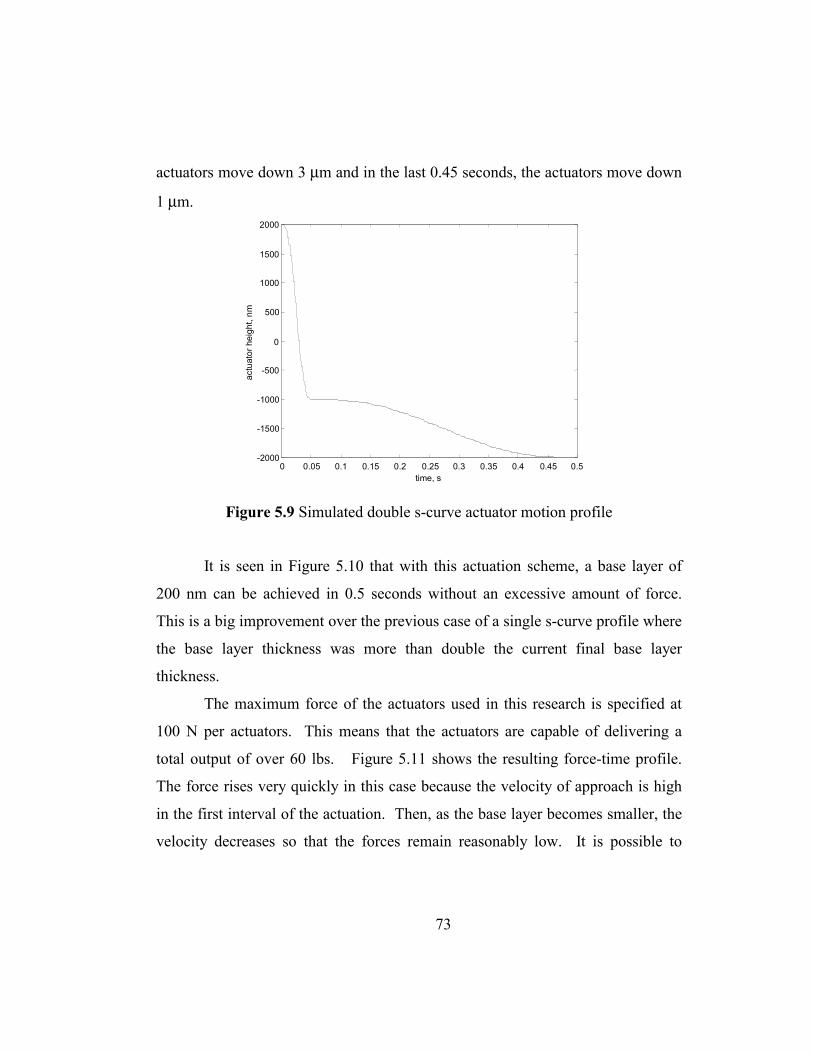
73

actuators move down 3 µm and in the last 0.45 seconds, the actuators move down

1 µm.

0 0.05 0.1 0.15 0.2 0.25 0.3 0.35 0.4 0.45 0.5 -2000

-1500

-1000

-500

0

500

1000

1500

2000

time, s

actu

ator

hei

ght,

nm

Figure 5.9 Simulated double s-curve actuator motion profile

It is seen in Figure 5.10 that with this actuation scheme, a base layer of

200 nm can be achieved in 0.5 seconds without an excessive amount of force.

This is a big improvement over the previous case of a single s-curve profile where

the base layer thickness was more than double the current final base layer

thickness.

The maximum force of the actuators used in this research is specified at

100 N per actuators. This means that the actuators are capable of delivering a

total output of over 60 lbs. Figure 5.11 shows the resulting force-time profile.

The force rises very quickly in this case because the velocity of approach is high

in the first interval of the actuation. Then, as the base layer becomes smaller, the

velocity decreases so that the forces remain reasonably low. It is possible to

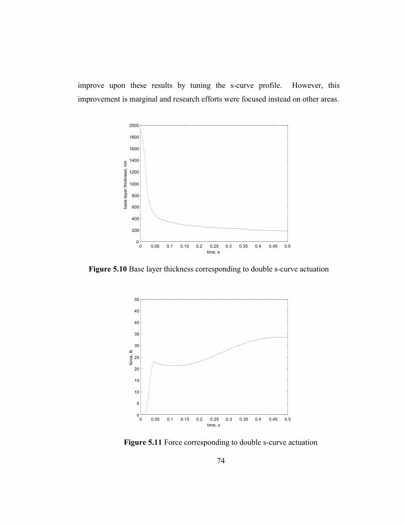
74

improve upon these results by tuning the s-curve profile. However, this

improvement is marginal and research efforts were focused instead on other areas.

0 0.05 0.1 0.15 0.2 0.25 0.3 0.35 0.4 0.45 0.5 0

200

400

600

800

1000

1200

1400

1600

1800

2000

time, s

base

laye

r thi

ckne

ss, n

m

Figure 5.10 Base layer thickness corresponding to double s-curve actuation

0 0.05 0.1 0.15 0.2 0.25 0.3 0.35 0.4 0.45 0.5 0 5

10 15 20 25 30 35 40 45 50

time, s

forc

e, lb

Figure 5.11 Force corresponding to double s-curve actuation

75

5.5 SQUEEZE FILM DYNAMICS OF PARALLEL, CIRCULAR PLATES

The analytical squeeze film damping force for parallel, circular plates was

applied to the equations of motion of the mechanical system. The analytical

equations for the fluid pressure for a parallel circular plate with a circular drop

from chapter 3 were applied to this simulation.

In this section, the results of a numerical simulation of the squeeze film

dynamics are presented. The results from numerous simulations show very

similar trends. The results presented here are nearly optimal when considering

final base layer thickness, required actuation forces, and the time to achieve the

desired base layer thickness. The results of the simulation in this section show

similar behavior as in the previous section where the solution of the two-

dimensional Reynolds equation was applied.

0 0.05 0.1 0.15 0.2 0.25 0.3 0.35 0.4 0.45 0.5 0 200 400 600 800

1000 1200 1400 1600 1800 2000

time, s

base

laye

r thi

ckne

ss, n

m

Figure 5.12 Base layer thickness corresponding to the case of finite, parallel circular plates

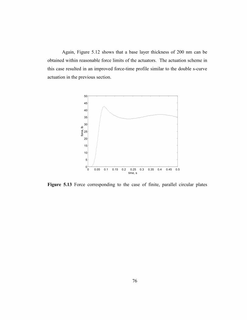
76

Again, Figure 5.12 shows that a base layer thickness of 200 nm can be

obtained within reasonable force limits of the actuators. The actuation scheme in

this case resulted in an improved force-time profile similar to the double s-curve

actuation in the previous section.

0 0.05 0.1 0.15 0.2 0.25 0.3 0.35 0.4 0.45 0.5 0 5

10 15 20 25 30 35 40 45 50

time, s

forc

e, lb

Figure 5.13 Force corresponding to the case of finite, parallel circular plates

77

Chapter 6: Experimental Results

6.1 INTRODUCTION

In order to verify the validity of the numerical simulations and

scientifically quantify the effects of the etch barrier layer on the dynamics of the

mechanical system, experiments were performed using the active stage prototype.

The data collected during the experiments included: 1) the motor shaft encoder

outputs from each of three high-resolution DC micrometer actuators, 2) the

dynamic force reading from each of three quartz force sensors mounted in series

with the actuators, and 3) gap sensing/film thickness measurements at two

locations across the template. The following sections discuss the process of

collecting this data and present the experimental results.

6.2 EXPERIMENTAL SETUP

6.2.1 Experimental Adaptations of the Active Stage Test Bed

Since a few of the subsystems of the active stage test bed have not been

fully implemented, a couple of adaptations were required to complete the

experiments and gather the necessary data. First, a wafer chuck system was not

readily available. In the active stage, the wafer chuck holds the spin-coated wafer

during the imprinting process and air solenoids pneumatically lift the wafer

towards the template stage. Thus, a temporary holding device to approximate the

semblance of an actual wafer chuck was designed and used. This component had

to be stiff in the lateral directions and hold the substrate close to the template

surface. It was designed to hold a 2.54 × 2.54 × 0.635 cm (1 × 1 × 1/4 inch)

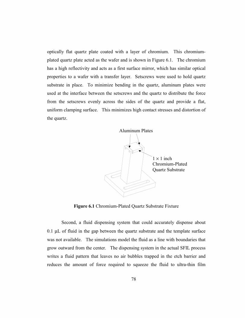
78

optically flat quartz plate coated with a layer of chromium. This chromium-

plated quartz plate acted as the wafer and is shown in Figure 6.1. The chromium

has a high reflectivity and acts as a first surface mirror, which has similar optical

properties to a wafer with a transfer layer. Setscrews were used to hold quartz

substrate in place. To minimize bending in the quartz, aluminum plates were

used at the interface between the setscrews and the quartz to distribute the force

from the setscrews evenly across the sides of the quartz and provide a flat,

uniform clamping surface. This minimizes high contact stresses and distortion of

the quartz.

Figure 6.1 Chromium-Plated Quartz Substrate Fixture

Second, a fluid dispensing system that could accurately dispense about

0.1 µL of fluid in the gap between the quartz substrate and the template surface

was not available. The simulations model the fluid as a line with boundaries that

grow outward from the center. The dispensing system in the actual SFIL process

writes a fluid pattern that leaves no air bubbles trapped in the etch barrier and

reduces the amount of force required to squeeze the fluid to ultra-thin film

1 × 1 inch Chromium-Plated Quartz Substrate

Aluminum Plates

79

thickness. Without the benefit of an accurate dispensing system, the next best

alternative was to completely fill the gap between the template and substrate.

The template is raised over 20 micron above the substrate, then water is dispensed

and fills the gap via capillary action.

Third, the etch barrier has the same viscosity as water so that water has the

same fluid mechanic effects as the etch barrier. This can be easily seen in the

incompressible Reynolds equation (see equation 2.10). The dominant fluid

property that affects the squeeze film pressure is viscosity. The different surface

tensions of the two fluids have a negligible effect in the overall squeeze film

pressure because when the fluid completely fills the gap, the boundary effects

become insignificant. Furthermore, working with etch barrier to perform squeeze

film experiments also poses unknown health risks without the use of the

automated dispensing system. Therefore, it was determined that water could be

used as a substitute for the etch barrier fluid.

6.2.2 Data Acquisition Hardware

The data acquisition hardware consists of an 800 MHz computer with a

National Instruments AT-MIO-16XE-50 data acquisition board capable of 20K

samples per second. The gap sensing system consists of an Ocean Optics®

SQ2000 four channel UV-VIS fiber optic spectrometer containing a 25 µm slit, a

600 line grating blazed at 500 nm, and 2048 pixel CCD array. The bandwidth of

the spectrometer is from 350 to 1000 nm. With a minimum 3-millisecond

integration time, this system has a maximum spectral acquisition rate of 300 Hz.

Two spectrometer channels were used to obtain film thickness results. Each fiber

80

optic probe was illuminated with a Tungsten-Halogen lamp. The broadband light

was focused onto the fiber optic probes with collimating lens.

The fiber optic probes are positioned with their axis spaced 0.7 inches

apart. A view of the physical setup is shown in Figure 6.2.

Figure 6.2 Physical layout of the experimental setup

6.2.3 Control Software

Control software for the experiment was developed using National

Instruments LabVIEW 6i. This control software was optimized for speed

during the data collection since the duration of actuation lasts only one second.

To collect enough data during this short duration, the sampling rate must be at

least 10 Hz. As mentioned above, the data acquisition is not limited by the

hardware. The sampling rates quoted by the manufacturers of the respective

Actuator/Encoder 2

Force Sensor 1

Force Sensor 2

Force Sensor 3

Actuator/Encoder 1

Actuator/Encoder 3

Fiber Optic Probe 2 Fiber Optic Probe 1

1 × 1 inch Quartz Template

Distributed Flexure Ring

Fixed to Support Frame

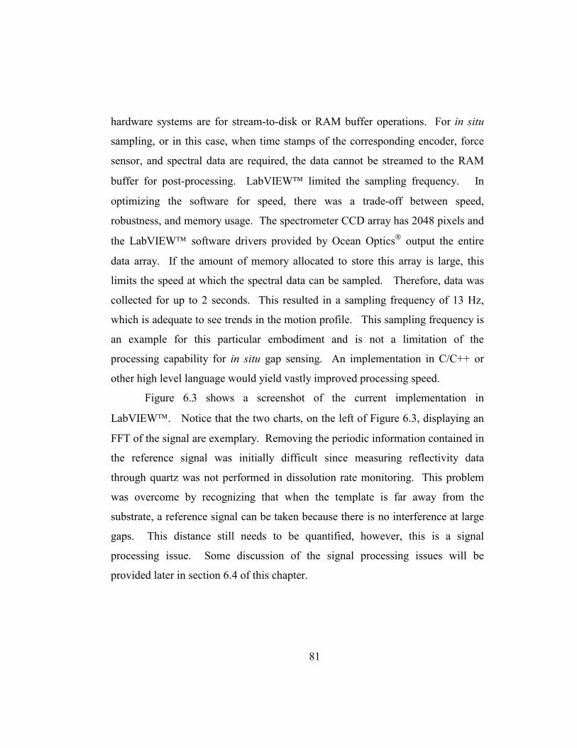
81

hardware systems are for stream-to-disk or RAM buffer operations. For in situ

sampling, or in this case, when time stamps of the corresponding encoder, force

sensor, and spectral data are required, the data cannot be streamed to the RAM

buffer for post-processing. LabVIEW limited the sampling frequency. In

optimizing the software for speed, there was a trade-off between speed,

robustness, and memory usage. The spectrometer CCD array has 2048 pixels and

the LabVIEW software drivers provided by Ocean Optics output the entire

data array. If the amount of memory allocated to store this array is large, this

limits the speed at which the spectral data can be sampled. Therefore, data was

collected for up to 2 seconds. This resulted in a sampling frequency of 13 Hz,

which is adequate to see trends in the motion profile. This sampling frequency is

an example for this particular embodiment and is not a limitation of the

processing capability for in situ gap sensing. An implementation in C/C++ or

other high level language would yield vastly improved processing speed.

Figure 6.3 shows a screenshot of the current implementation in

LabVIEW. Notice that the two charts, on the left of Figure 6.3, displaying an

FFT of the signal are exemplary. Removing the periodic information contained in

the reference signal was initially difficult since measuring reflectivity data

through quartz was not performed in dissolution rate monitoring. This problem

was overcome by recognizing that when the template is far away from the

substrate, a reference signal can be taken because there is no interference at large

gaps. This distance still needs to be quantified, however, this is a signal

processing issue. Some discussion of the signal processing issues will be

provided later in section 6.4 of this chapter.

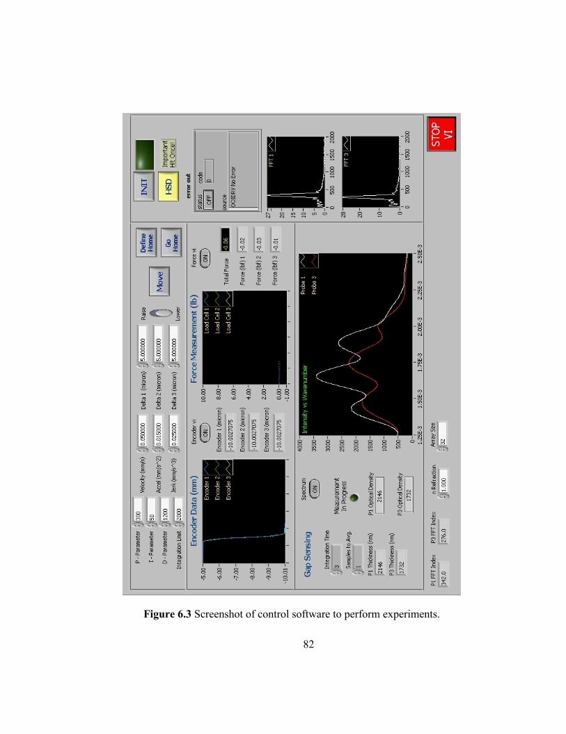
82

Figure 6.3 Screenshot of control software to perform experiments.

83

Also, as shown in Figure 6.3, the parameters passed to the LabVIEW

drivers for the motor controller are given in tables 6.1 and 6.2. The PID terms

were selected based on experimental tuning of the actuator outputs. The actual

motion profiles were visually compared against the desired motion output and the

PID terms were adjusted so that the desired and actual motions were closely

matched.

Parameter Recommended Range Actual

Proportional-Term 250 100 to 300 300

Integral-Term 12 0 to 50 50

Derivative-Term 800 0 to 1200 1200

Integration-Limit 2000 0 to 2000 2000

Table 6.1 PIDL parameters, recommended and actual settings for the C-842

Parameter Value

Velocity 0.05 mm/s

Acceleration 0.015 mm/s2

Jerk 0.025 mm/s2

Table 6.2 Parameters passed to the C-842 onboard s-curve profile generator6

6 The reader is referenced to the operating manuals from Physik Instrumente (PI).

84

6.3 EXPERIMENTAL PROCEDURE

Experiments were performed using the active stage prototype. Prior to

performing each experiment, the gap and angle of inclination was initialized with

air as the lubricating fluid in the gap. The alignment was performed by moving

the actuators independently until there were three or four fringes, which were

parallel to the center of rotation of the template holding stage. These fringes

could be easily seen and counted with the naked eye. Then the actuators were

uniformly raised by 20 micron and distilled water was dispensed into gap and

allowed to fill the gap completely. It was discovered in the course of the

experiments that particle contamination was a major factor contributing to the

quality of the experimental results. However, due to the lack of automation,

improved results could not be obtained within a reasonable time frame. Thus, the

experimental results presented in this thesis are meant to illustrate the trends in

the data.

It is noted that many more sets of data were taken than is shown here,

however due to the lack of automation, it was difficult to attain a controlled set of

initial conditions. Since the data sets have differing initial conditions, the data

cannot be easily compared or statistically analyzed. The data provided in this

thesis are meant to exemplify trends in the results as opposed to specific values.

6.4 EXPERIMENTAL RESULTS

6.4.1 Verification of the Simulation Results by Experiments

Several parameters were estimated in the modeling of the active stage

system. It was hypothesized that the composite axial stiffness parameter has a

higher amount of uncertainty than the other system parameters. Based on this,

85

the composite stiffness was calibrated using the results from one experimental

data set (known as the calibration set). The calibrated composite stiffness was

used to perform simulations that were then correlated to an independent set of

experimental results (known as the correlation set). From the simulation results,

it is inferred that the actual composite stiffness was less than previously

estimated. A comparison of the correlation set and the simulation supports the

hypothesis. The data show similar trends and are reasonably close. However,

there are still discrepancies, especially at large times, which may be due to

particles and other unknown parameters that have not been calibrated. These

issues require further investigation. The following details the process used in

calibrating the composite stiffness parameter.

A calibration simulation was performed taking initial conditions that

approximate the conditions for a specific set of measured data. With the fiber

optic spectrometer probes spaced 0.7 inches apart, the measured gap thickness for

each probe was 4780 nm and 2360 nm and the probe locations are assumed to be

symmetric about the center of rotation of the template holding mechanism. This

leads to an average height of 3570 nm with θ ~ 1.36 × 10-4 radians and total

actuation of 5 µm. These initial conditions were used to perform a simulation of

the squeeze film dynamics of the active stage system.

The composite axial stiffness and damping were systematically decreased

until the agreement between the film thickness from the experiments and the

simulations were within five percent. The axial stiffness was 1.5 × 106 N/m and

the damping constant was 75 N⋅s/m. The remaining system parameters in the

numerical simulation were taken from table 5.2. Figure 6.4 shows the data set

used in the calibration of the composite stiffness. The simulated film thickness

and the experimentally obtained film thickness values are within two percent.

86

0 0.1 0.2 0.3 0.4 0.5 0.6 0.7 0.8 0.9 1 2000 2200 2400 2600 2800 3000 3200 3400 3600 3800 4000

time, s

film

thic

knes

s, n

m

Figure 6.4 Average film thicknesses from simulation results (solid line) and experimental results (circles). Calibration set.

The trends in the motion for both the experimental results and the

simulation results are very similar. The influence of the s-curve actuation profile

is evident in Figure 6.4. At the beginning of the actuation where the velocity is

small, there is no change in the base layer thickness. As the actuators accelerate

downward, the base layer thickness decreases and the rate of sinkage of the

template is fairly constant. Then as the actuators slow down the rate of sinkage

also decreases and the base layer thickness levels off. It is observed in the

experiments that after the actuators stop moving, the base layer thickness continue

to decrease at a slow rate until the strain energy is minimized.

An encouraging result seen in both the experiments and the simulation is

that there is a corrective torque in the fluid damping that corrects the initial

angular misalignment of the template relative to the substrate. The angle of

inclination from simulation and experiments are in good agreement. This

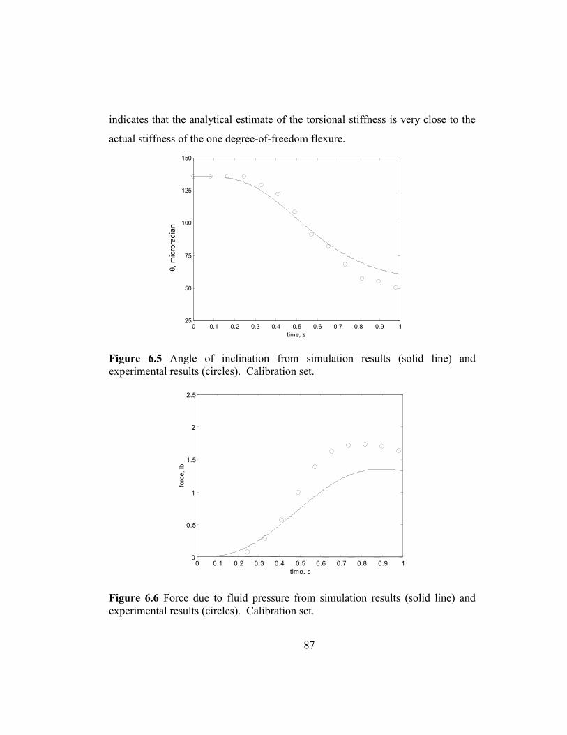
87

indicates that the analytical estimate of the torsional stiffness is very close to the

actual stiffness of the one degree-of-freedom flexure.

0 0.1 0.2 0.3 0.4 0.5 0.6 0.7 0.8 0.9 125

50

75

100

125

150

time, s

Figure 6.5 Angle of inclination from simulation results (solid line) and experimental results (circles). Calibration set.

0 0.1 0.2 0.3 0.4 0.5 0.6 0.7 0.8 0.9 1 0

0.5

1

1.5

2

2.5

time, s

forc

e, lb

Figure 6.6 Force due to fluid pressure from simulation results (solid line) and experimental results (circles). Calibration set.

θ, m

icro

radi

an

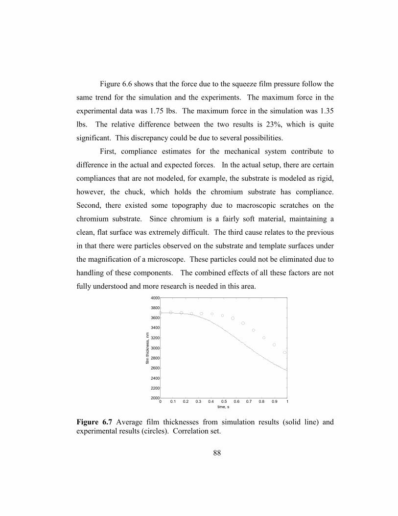
88

Figure 6.6 shows that the force due to the squeeze film pressure follow the

same trend for the simulation and the experiments. The maximum force in the

experimental data was 1.75 lbs. The maximum force in the simulation was 1.35

lbs. The relative difference between the two results is 23%, which is quite

significant. This discrepancy could be due to several possibilities.

First, compliance estimates for the mechanical system contribute to

difference in the actual and expected forces. In the actual setup, there are certain

compliances that are not modeled, for example, the substrate is modeled as rigid,

however, the chuck, which holds the chromium substrate has compliance.

Second, there existed some topography due to macroscopic scratches on the

chromium substrate. Since chromium is a fairly soft material, maintaining a

clean, flat surface was extremely difficult. The third cause relates to the previous

in that there were particles observed on the substrate and template surfaces under

the magnification of a microscope. These particles could not be eliminated due to

handling of these components. The combined effects of all these factors are not

fully understood and more research is needed in this area.

0 0.1 0.2 0.3 0.4 0.5 0.6 0.7 0.8 0.9 1 2000 2200 2400 2600 2800 3000 3200 3400 3600 3800 4000

time, s

film

thic

knes

s, n

m

Figure 6.7 Average film thicknesses from simulation results (solid line) and experimental results (circles). Correlation set.

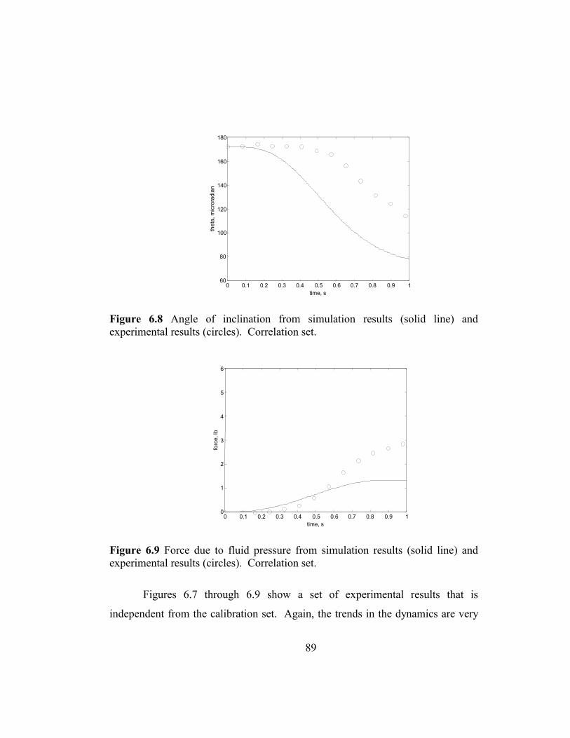
89

0 0.1 0.2 0.3 0.4 0.5 0.6 0.7 0.8 0.9 1 60

80

100

120

140

160

180

time, s

thet

a, m

icro

radi

an

Figure 6.8 Angle of inclination from simulation results (solid line) and experimental results (circles). Correlation set.

0 0.1 0.2 0.3 0.4 0.5 0.6 0.7 0.8 0.9 1 0

1

2

3

4

5

6

time, s

forc

e, lb

Figure 6.9 Force due to fluid pressure from simulation results (solid line) and experimental results (circles). Correlation set.

Figures 6.7 through 6.9 show a set of experimental results that is

independent from the calibration set. Again, the trends in the dynamics are very

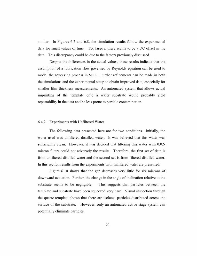
90

similar. In Figures 6.7 and 6.8, the simulation results follow the experimental

data for small values of time. For large t, there seems to be a DC offset in the

data. This discrepancy could be due to the factors previously discussed.

Despite the differences in the actual values, these results indicate that the

assumption of a lubrication flow governed by Reynolds equation can be used to

model the squeezing process in SFIL. Further refinements can be made in both

the simulations and the experimental setup to obtain improved data, especially for

smaller film thickness measurements. An automated system that allows actual

imprinting of the template onto a wafer substrate would probably yield

repeatability in the data and be less prone to particle contamination.

6.4.2 Experiments with Unfiltered Water

The following data presented here are for two conditions. Initially, the

water used was unfiltered distilled water. It was believed that this water was

sufficiently clean. However, it was decided that filtering this water with 0.02-

micron filters could not adversely the results. Therefore, the first set of data is

from unfiltered distilled water and the second set is from filtered distilled water.

In this section results from the experiments with unfiltered water are presented.

Figure 6.10 shows that the gap decreases very little for six microns of

downward actuation. Further, the change in the angle of inclination relative to the

substrate seems to be negligible. This suggests that particles between the

template and substrate have been squeezed very hard. Visual inspection through

the quartz template shows that there are isolated particles distributed across the

surface of the substrate. However, only an automated active stage system can

potentially eliminate particles.

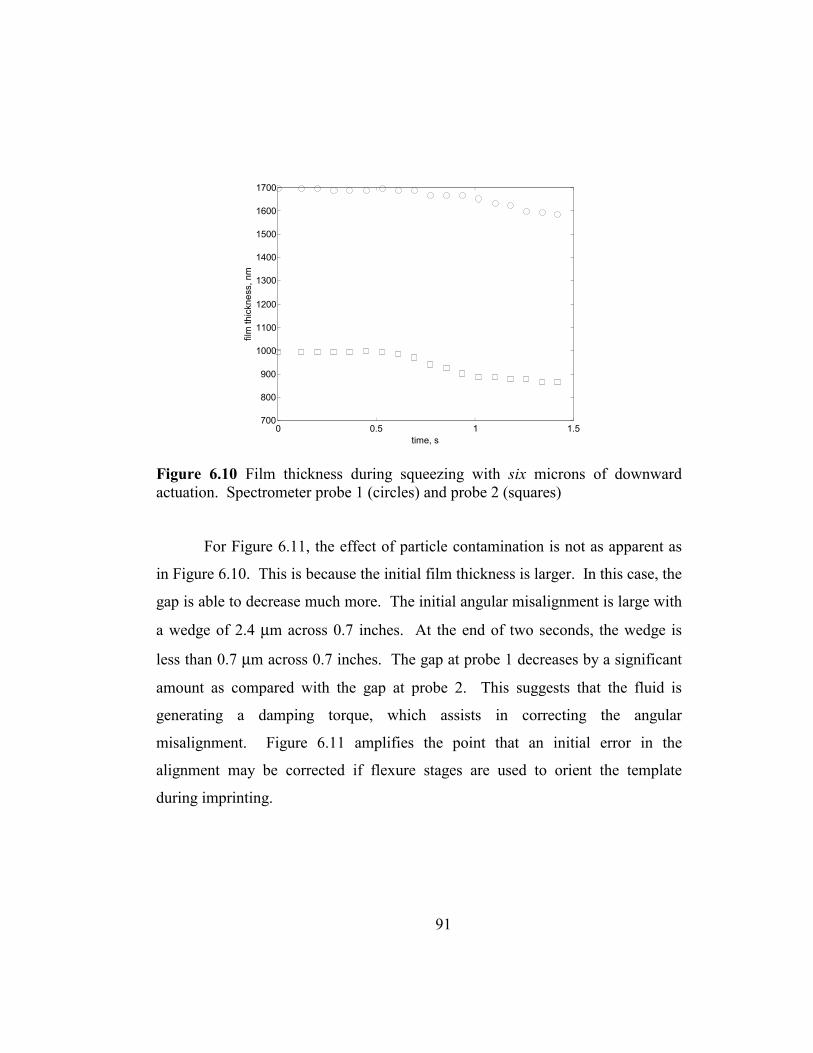
91

0 0.5 1 1.5 700 800 900

1000 1100 1200 1300 1400 1500 1600 1700

time, s

film

thic

knes

s, n

m

Figure 6.10 Film thickness during squeezing with six microns of downward actuation. Spectrometer probe 1 (circles) and probe 2 (squares)

For Figure 6.11, the effect of particle contamination is not as apparent as

in Figure 6.10. This is because the initial film thickness is larger. In this case, the

gap is able to decrease much more. The initial angular misalignment is large with

a wedge of 2.4 µm across 0.7 inches. At the end of two seconds, the wedge is

less than 0.7 µm across 0.7 inches. The gap at probe 1 decreases by a significant

amount as compared with the gap at probe 2. This suggests that the fluid is

generating a damping torque, which assists in correcting the angular

misalignment. Figure 6.11 amplifies the point that an initial error in the

alignment may be corrected if flexure stages are used to orient the template

during imprinting.

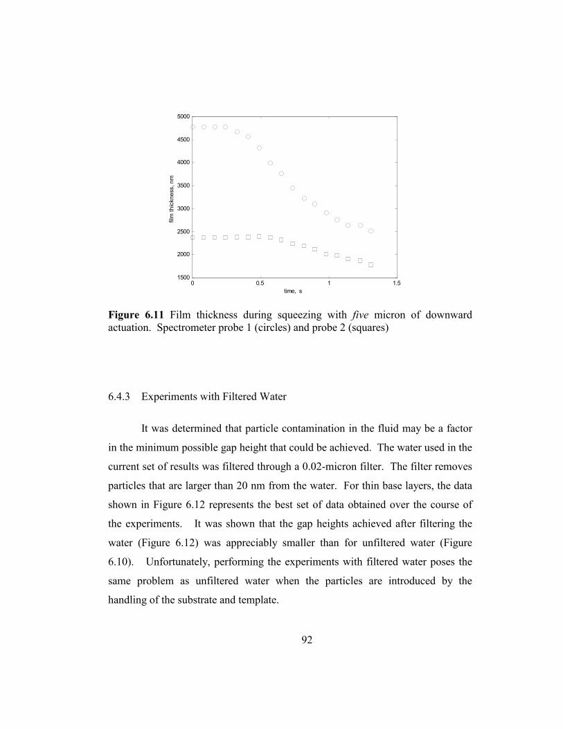
92

0 0.5 1 1.5 1500

2000

2500

3000

3500

4000

4500

5000

time, s

film

thic

knes

s, n

m

Figure 6.11 Film thickness during squeezing with five micron of downward actuation. Spectrometer probe 1 (circles) and probe 2 (squares)

6.4.3 Experiments with Filtered Water

It was determined that particle contamination in the fluid may be a factor

in the minimum possible gap height that could be achieved. The water used in the

current set of results was filtered through a 0.02-micron filter. The filter removes

particles that are larger than 20 nm from the water. For thin base layers, the data

shown in Figure 6.12 represents the best set of data obtained over the course of

the experiments. It was shown that the gap heights achieved after filtering the

water (Figure 6.12) was appreciably smaller than for unfiltered water (Figure

6.10). Unfortunately, performing the experiments with filtered water poses the

same problem as unfiltered water when the particles are introduced by the

handling of the substrate and template.

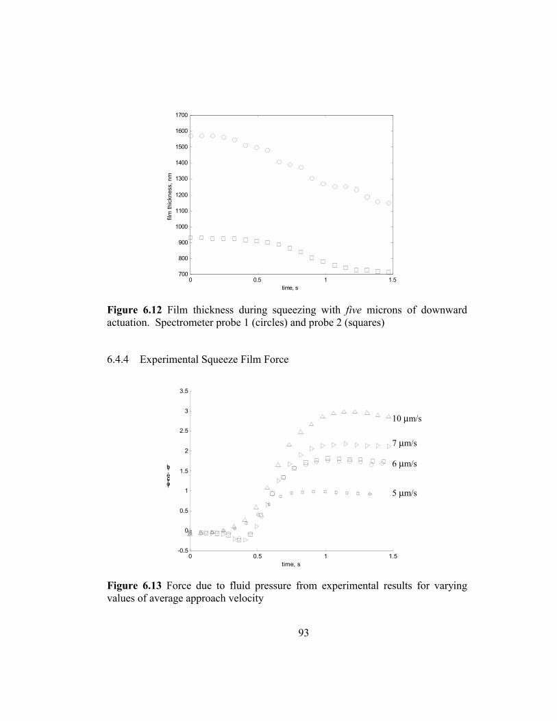
93

0 0.5 1 1.5 700 800 900

1000 1100 1200 1300 1400 1500 1600 1700

time, s

film

thic

knes

s, n

m

Figure 6.12 Film thickness during squeezing with five microns of downward actuation. Spectrometer probe 1 (circles) and probe 2 (squares)

6.4.4 Experimental Squeeze Film Force

0 0.5 1 1.5-0.5

0

0.5

1

1.5

2

2.5

3

3.5

time, s

force, lb

Figure 6.13 Force due to fluid pressure from experimental results for varying values of average approach velocity

10 µm/s

7 µm/s

6 µm/s

5 µm/s

94

Figure 6.13 shows the force-time plot for four different instances of

motion supplied by the actuators. In all of the cases, the actuators move for about

1 second. This translates into a higher average approach velocity. In Figure 6.13,

the maximum force due to the squeeze film pressure increases when the approach

velocity is higher. The force increases proportionally with the approach velocity,

but since the film thickness of each case is different, this increase in Figure 6.13

is not linear.

6.5 OBSERVATIONS AND DISCREPANCIES 6.5.1 Particle Contamination

Although the experiments were performed in a class 100 clean-room,

particle contamination was a fundamental problem in achieving the desired thin

fluid layers of 100 – 200 nm. During the course of the experimental work, it

became evident that is would not be possible to eliminate all particles without an

automated process. Particles could be caused by manual handling of the

experimental components. Furthermore, the fluid itself may have particles. The

water was filtered using 0.02-micron filters. This resulted in slight improvements

in the minimum attainable gaps. The substrate was placed under a microscope

with a magnification of 100× to detect particles. This was done immediately after

the substrate and template were cleaned in a solution of acetone followed by an

isopropyl alcohol rinse and a filtered air bath. A comparison with a clean wafer,

i.e. one that was not previously handled, showed that any handling beyond a

moving the wafer from its container to the imprinting machine would result in

particle contamination.

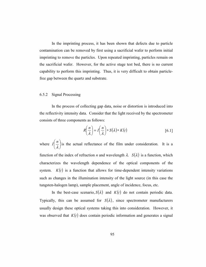
95

In the imprinting process, it has been shown that defects due to particle

contamination can be removed by first using a sacrificial wafer to perform initial

imprinting to remove the particles. Upon repeated imprinting, particles remain on

the sacrificial wafer. However, for the active stage test bed, there is no current

capability to perform this imprinting. Thus, it is very difficult to obtain particle-

free gap between the quartz and substrate.

6.5.2 Signal Processing

In the process of collecting gap data, noise or distortion is introduced into

the reflectivity intensity data. Consider that the light received by the spectrometer

consists of three components as follows:

( ) ( )tKSnInR ∗∗

=

λλλ

[6.1]

where

λnI is the actual reflectance of the film under consideration. It is a

function of the index of refraction n and wavelength λ. ( )λS is a function, which

characterizes the wavelength dependence of the optical components of the

system. ( )tK is a function that allows for time-dependent intensity variations

such as changes in the illumination intensity of the light source (in this case the

tungsten-halogen lamp), sample placement, angle of incidence, focus, etc.

In the best-case scenario, ( )λS and ( )tK do not contain periodic data.

Typically, this can be assumed for ( )λS , since spectrometer manufacturers

usually design these optical systems taking this into consideration. However, it

was observed that ( )tK does contain periodic information and generates a signal

96

in the FFT that is not indicative of the true signal

λnI . A method is proposed

for the minimization of the distortion introduced by ( )tK is described.

The intensity is normalized by a reference signal. It was observed that

the normalization of the intensity spectrum is very sensitive to the reference

spectrum. The reference spectrum should be at zero gap or film thickness and

through a material with the same index of refraction. However, if the reference

cannot be taken for these conditions, the Fourier transform of the intensity

spectrum will contain a false peak that belongs to the reference signal. This leads

to incorrect detection of the true signal since the magnitude of the reference is

dominant in this case.

Fortuitously, it was discovered that the intensity signal when the gap is

infinite, or practically speaking when interference is negligible, is identical to that

of zero gap. This allows the fiber optic probes to be placed at the measurement

locations and a reference to be taken through the quartz template. The template is

moved up from the substrate 100 microns and then a reference signal is captured.

Without this capability, taking a proper reference is not trivial since the reference

must be taken with the template removed and then the template must be put back

into to place before the experiment can proceed. However, in doing this, the

reference has been slightly modified because the index of refraction of quartz is

not unity, the sample placement has changed, and the measurement angle has

changed.

Height and angle of the probe also make a difference when obtaining the

reference signal. In the case of the reference, its period also changes as a function

of the optical path length. This is affected by the angle and focus of the signal.

Changes to these parameters can affect the measured gap thickness or lead to

failure in the FFT. Thus, the reference should be collected at large gap where the

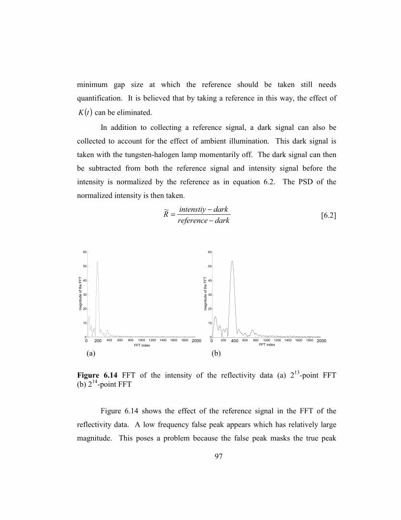
97

minimum gap size at which the reference should be taken still needs

quantification. It is believed that by taking a reference in this way, the effect of

( )tK can be eliminated.

In addition to collecting a reference signal, a dark signal can also be

collected to account for the effect of ambient illumination. This dark signal is

taken with the tungsten-halogen lamp momentarily off. The dark signal can then

be subtracted from both the reference signal and intensity signal before the

intensity is normalized by the reference as in equation 6.2. The PSD of the

normalized intensity is then taken.

darkreferencedarkenstiyintR−−=~ [6.2]

0 200 400 600 800 1000 1200 1400 1600 1800 20000

10

20

30

40

50

60

FFT index

mag

nitu

de o

f the

FFT

0 200 400 600 800 1000 1200 1400 1600 1800 20000

10

20

30

40

50

60

FFT index

mag

nitu

de o

f the

FFT

Figure 6.14 FFT of the intensity of the reflectivity data (a) 213-point FFT

(b) 214-point FFT

Figure 6.14 shows the effect of the reference signal in the FFT of the

reflectivity data. A low frequency false peak appears which has relatively large

magnitude. This poses a problem because the false peak masks the true peak

(a) (b)

98

when measuring thin layers in the range of about 300 to 400 nm. Figure 6.15

illustrates the case when a false peak masks the true peak. The difference

between 6.14a and 6.14b is that the number of zeros used to pad the FFT has been

increased by a power of two. This stretches the FFT out and the spectral leakage

is increased, however, note that the index at the maximum of the FFT has now

been approximately doubled. Spectral leakage is the smearing of energy across

the FFT domain, which results in wider peaks. This doubles the resolution since a

peak at an FFT index of 200.5, which cannot be resolved in 6.14a, is now equal to

a peak at an FFT index of 401 in 6.14b, for example.

0 1000 2000 3000 4000 5000 6000 7000 8000 90000 2 4 6 8

10 12 14 16 18 y g

FFT index

mag

nitu

de o

f the

FFT

Figure 6.15 False signal masking the true signal in FFT

6.5.3 Template/Substrate Deformation

The template and substrate can be deformed when using setscrews to

constrain their positions. The setscrews cause local stress concentrations that are

undesirable. This leads to possible bowing of the template and substrate. To

minimize the effect of stress concentrations on the bowing of the template and

substrate, flat aluminum plates were placed between the setscrews and the quartz

pieces.

False peak

True peak

99

Chapter 7: Closing Remarks 7.1 SUMMARY OF RESEARCH

This research has encompassed a broad range of areas including analytical

modeling, numerical simulations, and experimental analysis. It has also

incorporated a medley of software/hardware issues and spectral analysis. By

interpreting the analytical models, numerical simulations, and experimental

results, it has been shown that the Reynolds equations for squeeze film damping

is a valid and useful tool for understanding the dynamics of the mechanical

systems in SFIL.

The fluid pressure plays a significant role to orient the passively compliant

stages used in the multi-imprint stepper and the single imprint machines. It has

been shown that the pressure tends to correct the angular misalignments by

generating a damping torque and the pressure asymmetry cannot be ignored.

Thus, the original intent of the passive stage designs has been proven to work.

The passive stages self-correct due to the coupling between the mechanical

system and the liquid etch barrier. Although presence of the etch barrier aides in

correcting the misalignment, it also limits the rate at which imprinting can be

done since, thinner base layers require more time to achieve. However, with an

appropriate control scheme, based on a two s-curve motion profile, this problem

can be solved. Furthermore, the theoretical and measured forces can be achieved

by the actuation systems currently implemented.

An additional contribution of this research work has been the application

of a real-time gap-sensing tool in measuring the film thickness of the fluid during

the squeezing process. In developing an active stage system to perform SFIL, this

100

is a major milestone. The next step would be to use this information to perform

real-time control of the base layer thickness and template orientation.

Step and Flash imprint lithography has the potential to become a

manufacturing technology within several years. It offers high-resolution

capability, high-throughput, and cost effectiveness. Much progress has been

made in the way of appropriate chemistries for the etch barrier, transfer layers,

etc. Significant work has been done to understand the kinematics of the machines

necessary to perform imprinting. Several imprinting prototypes have been

developed and are currently being used to meet the ongoing challenges in the

research. There are several milestones that must be surpassed before SFIL can

become a full manufacturing technology. The following sections attempt to

illuminate the reader on these specific tasks.

7.2 FUTURE WORK

7.2.1 Numerical Solution to the Generalized Reynolds Equation

In deriving the analytical solution to the pressure distribution, the

topography of the template has been neglected. Also, three-dimensional effects

could be significant enough to warrant a full numerical solution to the generalized

Reynolds equation, which would include topography, growth of the fluid

boundary, and angle of inclination as well as lateral motions. A practical issue in

modeling with the generalized solution to the Reynolds equation is computational

complexity since the solution would need to be numerical as opposed to

analytical. Complete fluid-structure coupling may require a high number of

floating-point operations and complex numerical algorithms to solve for the

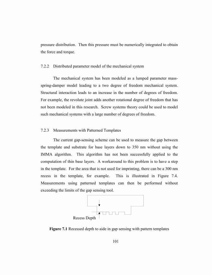
101

pressure distribution. Then this pressure must be numerically integrated to obtain

the force and torque.

7.2.2 Distributed parameter model of the mechanical system

The mechanical system has been modeled as a lumped parameter mass-

spring-damper model leading to a two degree of freedom mechanical system.

Structural interaction leads to an increase in the number of degrees of freedom.

For example, the revolute joint adds another rotational degree of freedom that has

not been modeled in this research. Screw systems theory could be used to model

such mechanical systems with a large number of degrees of freedom.

7.2.3 Measurements with Patterned Templates

The current gap-sensing scheme can be used to measure the gap between

the template and substrate for base layers down to 350 nm without using the

IMMA algorithm. This algorithm has not been successfully applied to the

computation of thin base layers. A workaround to this problem is to have a step

in the template. For the area that is not used for imprinting, there can be a 300 nm

recess in the template, for example. This is illustrated in Figure 7.4.

Measurements using patterned templates can then be performed without

exceeding the limits of the gap sensing tool.

Figure 7.1 Recessed depth to aide in gap sensing with pattern templates

Recess Depth

102

7.2.4 Control scheme

The ultimate goal of an active stage system is to actively control the

orientation of the template relative to the substrate. A better understanding of the

fluid mechanical effects gives insight in the process of developing a feedforward

or feedback control system. In a feedback control scheme, the controller would

take as input the gap sensing information and perform real-time control at 10 Hz

or better. Ultra-high resolution, high bandwidth actuation can be supplied by

piezoelectric actuators, which are capable of nanometer resolution motions.

103

Appendix A: Axisymmetric Problem

The Reynolds equation for the geometry of a flat, circular plate

approaching a flat surface is given as

dtdhrph

rrprh

rµ

θθ121 33 =

∂∂

∂∂+

∂∂

∂∂ . [A.1]

If the plate is parallel as it approaches the surface, then for a drop fluid

with radius rb, axial symmetry exists and the pressure is only a function of the

radius. Thus in the case of an axisymmetric squeeze film, the Reynolds equation

is given as

dtdhr

drdprh

drd µ123 =

. [A.2]

Integrating gives

A

dtdhr

drdprh += 23 6µ . [A.3]

Dividing through,

33

6rhA

dtdh

hr

drdp += µ , [A.4]

and since ∞≠drdp when 0=r then 0=A . Hence,

dtdh

hr

drdp

3

6µ= , [A.5]

and a further integration gives

B

dtdh

hrp += 3

23µ . [A.6]

104

Assuming the liquid perfectly wets the surfaces of the plate and substrate,

i.e., zero contact angle, the pressure at the boundary is given by h

p γ2−= when

brr = . Therefore dtdh

hr

hB b

3

232 µγ −−= .

( )hdt

dhh

rrp b γµ 233

22 −−= [A.7]

The force is given by the integration of the pressure in the r and θ directions

( )∫ ∫=π

θ2

0 0

br drdrrpF . [A.8]

Integrating with respect to r and θ, the squeeze film force is then

−−=

hr

dtdh

hr

F bb2

3

4

43

2γµπ . [A.9]

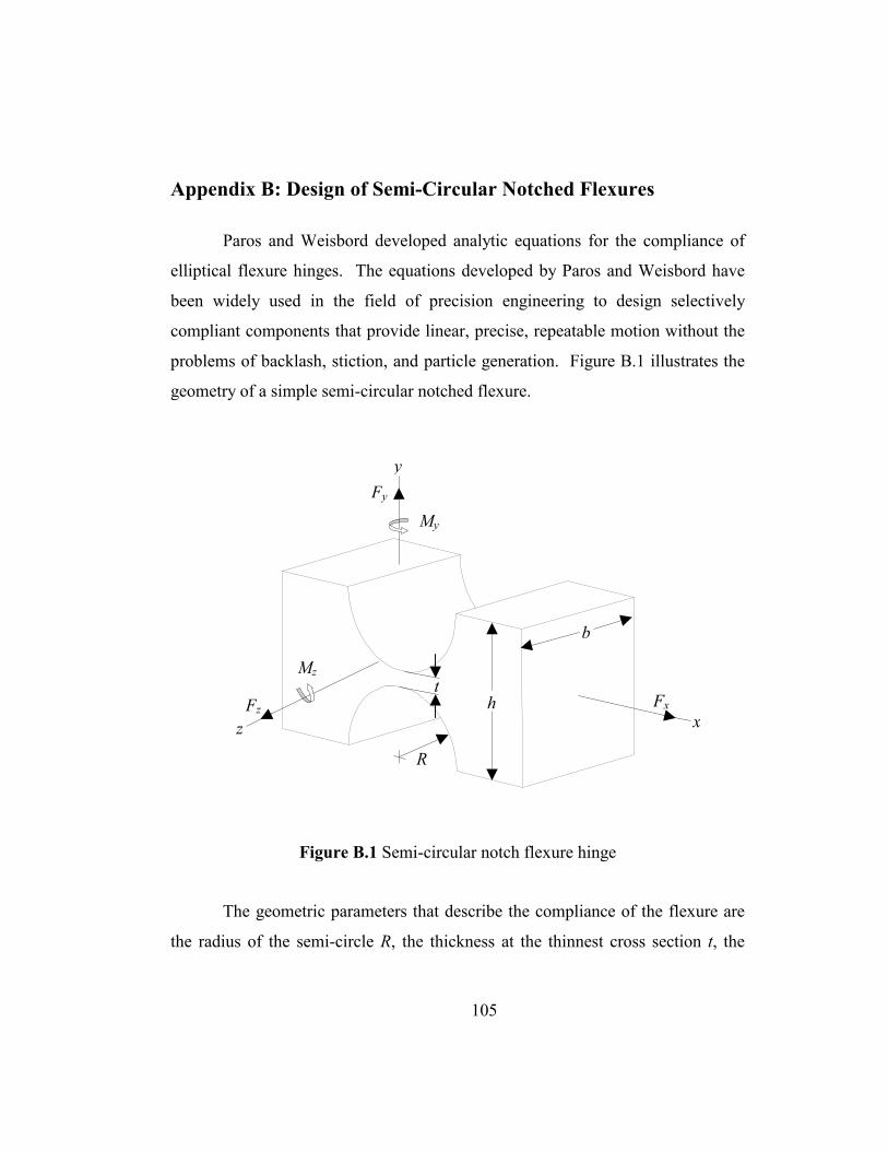
105

Appendix B: Design of Semi-Circular Notched Flexures

Paros and Weisbord developed analytic equations for the compliance of

elliptical flexure hinges. The equations developed by Paros and Weisbord have

been widely used in the field of precision engineering to design selectively

compliant components that provide linear, precise, repeatable motion without the

problems of backlash, stiction, and particle generation. Figure B.1 illustrates the

geometry of a simple semi-circular notched flexure.

Figure B.1 Semi-circular notch flexure hinge

The geometric parameters that describe the compliance of the flexure are

the radius of the semi-circle R, the thickness at the thinnest cross section t, the

h

b

My

Mz

Fy

Fx Fz

z

y

x

t

R

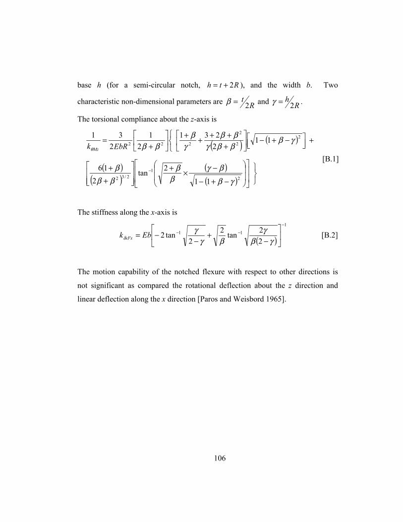
106

base h (for a semi-circular notch, Rth 2+= ), and the width b. Two

characteristic non-dimensional parameters are Rt2=β and R

h2=γ .

The torsional compliance about the z-axis is

( ) ( ) +

−+−

+++++

+= 11

2231

21

231 2

2

2

222 γβββγββ

γβ

ββθ EbRk Mz

( )( )

( )( )

−+−

−×+

++ −

2

12/32 11

2tan2

16

γβ

βγββ

βββ

[B.1]

The stiffness along the x-axis is

( )

1

11

22tan2

2tan2

−

−−

−+

−−=

γβγ

βγγ

δ Ebk xFx [B.2]

The motion capability of the notched flexure with respect to other directions is

not significant as compared the rotational deflection about the z direction and

linear deflection along the x direction [Paros and Weisbord 1965].

107

References

Bailey, T., B. J. Choi, M. Colburn, M. Meissl, S. Shaya, J.G. Ekerdt, S.V. Sreenivasan, and C.G. Willson. 2000. Step and flash imprint lithography: Template surface treatment and defect analysis. J. Vac. Sci. Technol. B 18(6): 3572-77.

Bhushan, B. Principles and Applications of Tribology. New York: John Wiley & Sons, 1999.

Bhushan, B. Handbook of Micro/Nano Tribology. New York: CRC Press, 1995.

Bouldin, C.E., W. E. Wallace, G.W. Lynn, S.C. Roth, and W.L. Wu. 2000. Thermal expansion coefficients of low-k dielectric films from Fourier analysis of x-ray reflectivity. J. Appl. Phys., 88(2): 691-95.

Cameron, A. Basic Lubrication Theory. New York: John Wiley & Sons, 1976.

Chalmers, S. United States Patent No. 6,204,922 B1 Issued: 3/2001. Rapid and accurate thin film measurement of individual layers in a multi-layered or patterned sample. Assignee: Filmetrics, Inc., San Diego, CA.

Chason, E. 2000. Use of kSA MOS system for stress and thickness monitoring during CVD growth. Brown University.

Choi, B. J., S. Johnson, and S.V. Sreenivasan. 1999. A high resolution imprint lithography machine for patterning flat and curved substrates, Department of Mechanical Engineering, The University of Texas at Austin. DARPA Interim Report.

Choi, B.J, S. Johnson, S.V. Sreenivasan, M. Colburn, T. Bailey, and C.G. Willson. 2000. Partially constrained compliant stages for high resolution imprint lithography. Proceedings of DETC 2000: ASME Design Engineering Technical Conference, Baltimore, MD.

108

Chou, S. Y., P .R. Krauss, and P. J. Renstrom. 1996. Nanoimprint lithography. J. Vac. Sci. Technol B 14(6): 4129-33.

Colburn, M. “Step and Flash Imprint Lithography: A Low-Pressure, Room Temperature Nanoimprint Lithography.” Ph.D. dissertation, The University of Texas at Austin, 2001.

Colburn, M., S. Johnson, M. Stewart, S. Damle, T. Bailey, B. Choi, M. Wedlake, T. Michaelson, S.V. Sreenivasan, J. Ekerdt, and C. G. Willson. Step and flash imprint lithography: A novel approach to imprint lithography. SPIE 1999 Annual International Symposium on Microlithography.

Collis, S. S. An Introduction to Numerical Analysis for Computational Fluid Mechanics. Course notes. Department of Mechanical Engineering and Materials Science, Rice University, Houston, TX, 2000.

Freeland, A. C. “Mathematical modeling of the dynamics and production of biosensors.” Ph.D. dissertation, The University of Texas at Austin, 2000.

Haisma, J., M. Verheijan, K. Heuvel, and J. Berg. 1996. Mold-assisted nanolithography: A process for reliable pattern replication. J. Vac. Sci Technol. B 14(6): 4124-28.

Hays, D.F. 1962. Squeeze films for rectangular plates. ASME Paper No. 62-Lub-

S-9.

Huibers, P. 1997. Models for the wavelength dependence of the index of refraction of water. Applied Optics. 36(16): 3785-87.

Johnson, S.C. 1999. Selectively compliant orientation stages for imprint lithography. M.S. Thesis, Mechanical Engineering, The University of Texas, Austin.

109

Miller, R. E., P. Bischoff, R. Sumner, S. Bowler, W. Flack, and G. Fong. The Development of 157nm Small Field and Mid-Field MicroSteppers. SPIE 2000 Annual International Symposium on Microlithography.

Moore, D. F. 1965. A review of squeeze films. Wear 8:245-63.

Moore, D. F. 1964. On the inclined non-inertial sinkage of a flat plate. J. Fluid

Mech. 20(2):321-30.

Muzio, E., P. Seidel, M. Mason, J. Canning, and Gil Sheldon. Lithography Cost of Ownership Analysis Revision Number: 4.0 Revision Date: December 1999. www.sematech.org/public/resources/coo/index.htm

Paros, J.M. and L. Weisbord. 1965. How to design flexure hinges. Machine Design No. T-27, pp. 151-156.

Patir, N. and H. S. Cheng. 1978. An average flow model for determining the effects of three-dimensional roughness on partial hydrodynamic lubrication. J. Lub. Technol. 100:12-17.

Sakurai, K. and A. Iida. 1992. Fourier analysis of interference structure in x-ray specular reflection from thin films. Jpn. J. Appl. Phys. 31:L113-L115.

Sheats, J. and B. Smith. Microlithography: Science and Technology. New York: Marcel Dekker, 1998.

Stulen, R.H. and D. W. Sweeney. 1999. Extreme Ultraviolet Lithography. IEEE J. Quantum Electronics 35(5):694-699.

Thompson, L. F., C. G. Willson, and M. J. Bowen. Introduction to Microlithography, 2nd Edition, ACS Professional Reference Book. Washington, D. C.: American Chemical Society, 1994.

110

Tripp, J. H. 1983. Surface roughness effects in hydrodynamic lubrication: The flow factor method. J. Lub. Techol. 105:458-65.

Wang, D., S. G. Thomas, K. L. Wang, Y. Xia, and G. M. Whitesides. 1997. Nanometer scale patterning and pattern transfer on amorphous Si, crystalline Si, and SiO2 surfaces using self-assembled monolayers. Appl. Phys. Lett. 70(12): 1593-95.

Whidden, T. K., D. K. Ferry, M. N. Kozicki, E. Kim, A. Kumar, J. Wilbur, and G. M. Whitesides. 1996. Pattern transfer to silicon by microcontact printing and RIE. Nanotechnology 7: 447-51.

111

Vita Anh Quoc Nguyen was born in Vungtau, Vietnam on July 22, 1976, the

eldest son of Mai Thi Dinh and Ban Van Nguyen, deceased. After completing his

work at Rockport-Fulton High, Rockport, Texas, in 1995, he entered Rice

University in Houston, Texas. He received the degree of Bachelor of Science in

Mechanical Engineering from Rice University in May 1999. In September 1999,

he entered The Graduate School at The University of Texas at Austin.

Permanent Address: 108 North Twelfth Street

P.O. Box 117

Fulton, Texas 78358

This thesis was typed by the author.