copyright 2016, theeradej suabtrirat
TRANSCRIPT

THREE ESSAYS ON HIGH-SPEED INTERNET: HOME AND MOBILE
INTERNET ADOPTION, THE EFFECT OF INTERNET’S PRICE AND SPEED,
AND WELFARE EVALUATION
by
THEERADEJ SUABTRIRAT, BBA
A DISSERTATION
IN
ECONOMICS
Submitted to the Graduate Faculty
of Texas Tech University in
Partial Fulfillment of
the Requirements for
the Degree of
DOCTOR OF PHILOSOPHY
Approved
Robert McComb, PhD
Chair of Committee
Terry Von Ende, PhD
Masha Rahnamamoghadam, PhD
Benaissa Chidmi, PhD
Mark Sheridan, PhD
Dean of the Graduate School
May 2016

Copyright 2016, Theeradej Suabtrirat

Texas Tech University, Theeradej Suabtrirat, May 2016
ii
ACKNOWLEDGMENTS
Completing a dissertation is a long journey, and I have reached the destination
by the strong support of many people around me. First, I would like to thank Dr.
McComb for his chairing my dissertation. He has given me encouragement, valuable
guidance, and marketable research topics. I will remember him as a role model when I
become a professor in the near future. Second, I would like to thank Dr. Chidmi for his
help in verifying the validity of my econometric results. Third, I would like to thank
Dr. Von Ende and Dr. Rahnamamoghadam for serving as my dissertation committee
and offering useful insights, as well as Dr. Khan for serving as the graduate school
representative of my dissertation. Fourth, I would like to thank Dr. Boonsaeng, Dr.
Carpio, and Dr. Noel for valuable comments to improve my dissertation.
Next, I would like to thank Dr. Becker, Dr. Al-Hmoud, and the Department of
Economics for the opportunity to teach an undergraduate class and for a teaching
assistantship for the completion of my PhD study. Moreover, I would like to thank the
Snyder Communication Skills Center of the Rawls College of Business for editing and
revising my dissertation. Furthermore, I would like to thank my parents, my brother,
and my loved ones for motivating me when I was tempted to give up. Lastly, I would
like to dedicate this work to my late grandmother who raised me when I was a little
naughty boy.

Texas Tech University, Theeradej Suabtrirat, May 2016
iii
TABLE OF CONTENTS
ACKNOWLEDGEMENTS .................................................................................................. ii
ABSTRACT ...................................................................................................................... v
LIST OF TABLES ............................................................................................................ vi
LIST OF FIGURES .......................................................................................................... xi
CHAPTER I: INTRODUCTION ......................................................................................... 1
CHAPTER II: HOME AND MOBILE INTERNET ADOPTION ............................................. 4
Introduction ................................................................................................................ 4
Home Internet Adoption ............................................................................................ 5
Literature Review ................................................................................................... 9
Model ................................................................................................................... 12
Data Sources......................................................................................................... 14
Results .................................................................................................................. 15
Mobile Internet Adoption ......................................................................................... 19
Literature Review ................................................................................................. 22
Model ................................................................................................................... 25
Data Sources......................................................................................................... 25
Results .................................................................................................................. 26
Conclusion ............................................................................................................... 31
CHAPTER III: THE EFFECT OF INTERNET’S PRICE AND SPEED ................................. 32
Introduction .............................................................................................................. 32
Literature Review ..................................................................................................... 33
Model ....................................................................................................................... 37
Data Sources............................................................................................................. 40
Results ...................................................................................................................... 45
Results on the Effect of Internet’s Monthly Price and Download Speed ............ 46
Results on Own and Cross Price Effect ............................................................... 52
Results on Own and Cross Price Elasticity .......................................................... 54
Conclusion ............................................................................................................... 57

Texas Tech University, Theeradej Suabtrirat, May 2016
iv
CHAPTER IV: WELFARE EVALUATION ....................................................................... 59
Introduction .............................................................................................................. 59
Literature Review ..................................................................................................... 60
Model ....................................................................................................................... 64
Data Sources............................................................................................................. 67
Results ...................................................................................................................... 71
Results on Welfare Change from Decreased Monthly Price ............................... 71
Results on Welfare Change from Faster Download Speed .................................. 82
Conclusion ............................................................................................................... 92
Appendix .................................................................................................................. 94
CHAPTER V: POLICY IMPLICATIONS ......................................................................... 110
Solutions Supported by the Results of this Dissertation ........................................ 110
Overcoming Digital Literacy Barriers ............................................................... 110
Overcoming Cost Barriers.................................................................................. 111
Overcoming Irrelevance Barriers ....................................................................... 112
Overcoming Language Barriers ......................................................................... 112
Overcoming Accessibility Barriers .................................................................... 113
Solutions Supported by the Findings of Previous Literature ................................. 114
Overcoming Low Internet Adoption in Low Income Areas .............................. 114
Overcoming Insufficient Infrastructure in Rural Areas ..................................... 114
Expanding Availability of Information Technology Employment .................... 115
Conclusion ............................................................................................................. 115
BIBLIOGRAPHY .................................................................................................... 117

Texas Tech University, Theeradej Suabtrirat, May 2016
v
ABSTRACT
The Internet brings substantial benefits to American households. This
dissertation studies the internet adoption of American households and divides its
presentation into three essays as follows.
The first essay analyzes the effect of demographic and geographic
characteristics of American households on the probability of home and mobile internet
adoption. The data source of this essay is the Current Population Survey Computer
and Internet Use Supplement July 2013. Using the binary logit model, the results
indicate that 1) the internet adoption rates tend to be higher for households with better
education, higher family income, younger adults, school-age children, and urban
residence; and 2) the home and mobile internet models have different sizes of
marginal effects for several household characteristics.
The second essay investigates the effect of the internet service’s monthly price
and download speed and the household’s characteristics on the choice of home
internet service of the households in four U.S. cities (Los Angeles, San Francisco,
Washington, DC, and New York City). This essay merges the Current Population
Survey Computer and Internet Use Supplement July 2013 with the Cost of
Connectivity 2013 dataset. Using the mixed logit model, the results indicate that 1)
households tend to purchase the internet package that offers faster download speed at a
more affordable price; 2) the demand for internet services is price-elastic; and 3)
households with better education, higher family income, and younger adults are more
likely to purchase high-speed internet service than households with opposite qualities.
The third essay quantifies the amount of welfare improvement and predicts an
increase in internet adoption rate from cheaper internet price and faster internet speed.
The data sources of this essay are the same as those of the second essay. Using the
log-sum difference method, the results demonstrate that households with better
education, higher family income, and younger adults tend to have higher internet
adoption rates and earn larger amounts of compensated variation than households with
opposite characteristics.

Texas Tech University, Theeradej Suabtrirat, May 2016
vi
LIST OF TABLES
Table 1: Home Computer, Internet, and Broadband Adoption by
Demographic Characteristics. .............................................................. 10
Table 2: Logistic Regression of Home Internet Adoption on
Household's and Householder's Characteristics ................................... 16
Table 3: Smartphone Owners in 2014 by Demographic Characteristics ..................... 23
Table 4: Marginal Effects of Demographics on Selected Mobile Phone
Activities. ............................................................................................. 24
Table 5: Logistic Regression of Mobile Internet Adoption on
Household's and Householder's Characteristics ................................... 27
Table 6: The List of Important Variables. .................................................................... 42
Table 7: The List of Internet Packages in Los Angeles ............................................... 44
Table 8: The List of Internet Packages in San Francisco ............................................. 44
Table 9: The List of Internet Packages in Washington, DC ........................................ 45
Table 10: The List of Internet Packages in New York City ......................................... 45
Table 11: The Result of the Mixed Logit Regression of Households'
Choice on Internet Package's and Household's
Characteristics in Los Angeles and San Francisco Area. ..................... 48
Table 12: The Result of the Mixed Logit Regression of Households'
Choice on Internet Package's and Household's
Characteristics in Washington, DC and New York City
Area. ..................................................................................................... 50
Table 13: Own and Cross Price Effect of Internet Packages in Los
Angeles (in Probability Unit). .............................................................. 53
Table 14: Own and Cross Price Effect of Internet Packages in San
Francisco (in Probability Unit)............................................................. 53
Table 15: Own and Cross Price Effect of Internet Packages in
Washington, DC (in Probability Unit). ................................................ 54
Table 16: Own and Cross Price Effect of Internet Packages in New
York City (in Probability Unit). ........................................................... 54
Table 17: Own and Cross Price Elasticity of Internet Packages in Los
Angeles (in Rate of Change of Probability). ........................................ 56

Texas Tech University, Theeradej Suabtrirat, May 2016
vii
Table 18: Own and Cross Price Elasticity of Internet Packages in San
Francisco (in Rate of Change of Probability). ..................................... 56
Table 19: Own and Cross Price Elasticity of Internet Packages in
Washington DC (in Rate of Change of Probability). ........................... 57
Table 20: Own and Cross Price Elasticity of Internet Packages in New
York City (in Rate of Change of Probability). ..................................... 57
Table 21: Group of Variables for Welfare Evaluation by Household’s
and Internet Package’s Characteristics................................................. 67
Table 22: The List of Internet Packages in Los Angeles (after Speed
Group Assignment) .............................................................................. 69
Table 23: The List of Internet Packages in San Francisco (after Speed
Group Assignment) .............................................................................. 69
Table 24: The List of Internet Packages in Washington, DC (after
Speed Group Assignment) ................................................................... 70
Table 25: The List of Internet Packages in New York City (after Speed
Group Assignment) .............................................................................. 70
Table 26: The Means of Compensated Variation (CV) and Expected
Adoption Increase (Percentage in Parenthesis) from a
$10 Decrease in Monthly Price for Los Angeles
Households Categorized by Family Annual Income
Levels. .................................................................................................. 72
Table 27: The Means of Compensated Variation (CV) and Expected
Adoption Increase (Percentage in Parenthesis) from a
$10 Decrease in Monthly Price for Los Angeles
Households Categorized by Education Levels of
Householders. ....................................................................................... 75
Table 28: The Means of Compensated Variation (CV) and Expected
Adoption Increase (Percentage in Parenthesis) from a
$10 Decrease in Monthly Price for Los Angeles
Households Categorized by Age Levels Of
Householders. ....................................................................................... 76
Table 29: The Means of Compensated Variation (CV) and Expected
Adoption Increase (Percentage in Parenthesis) from a
$10 Decrease in Monthly Price for San Francisco
Households Categorized by Family Annual Income
Levels. .................................................................................................. 77

Texas Tech University, Theeradej Suabtrirat, May 2016
viii
Table 30: The Means of Compensated Variation (CV) and Expected
Adoption Increase (Percentage in Parenthesis) from a
$10 Decrease in Monthly Price for San Francisco
Households Categorized by Education Levels of
Householders. ....................................................................................... 78
Table 31: The Means of Compensated Variation (CV) and Expected
Adoption Increase (Percentage in Parenthesis) from a
$10 Decrease in Monthly Price for San Francisco
Households Categorized by Age Levels of
Householders. ....................................................................................... 78
Table 32: The Means of Compensated Variation (CV) and Expected
Adoption Increase (Percentage In Parenthesis) from a
$10 Decrease in Monthly Price for Washington, DC
Households Categorized by Family Annual Income
Levels. .................................................................................................. 79
Table 33: The Means of Compensated Variation (CV) and Expected
Adoption Increase (Percentage In Parenthesis) from a
$10 Decrease In Monthly Price for Washington, DC
Households Categorized by Education Levels of
Householders. ....................................................................................... 79
Table 34: The Means of Compensated Variation (CV) and Expected
Adoption Increase (Percentage in Parenthesis) from a
$10 Decrease in Monthly Price for Washington, DC
Households Categorized by Age Levels of
Householders. ....................................................................................... 80
Table 35: The Means of Compensated Variation (CV) and Expected
Adoption Increase (Percentage in Parenthesis) from a
$10 Decrease in Monthly Price for New York City
Households Categorized by Family Annual Income
Levels. .................................................................................................. 80
Table 36: The Means of Compensated Variation (CV) and Expected
Adoption Increase (Percentage in Parenthesis) from a
$10 Decrease in Monthly Price for New York City
Households Categorized by Education Levels ..................................... 81
Table 37: The Means of Compensated Variation (CV) and Expected
Adoption Increase (Percentage in Parenthesis) from a
$10 Decrease in Monthly Price for New York City
Households Categorized by Age Levels of
Householders. ....................................................................................... 81

Texas Tech University, Theeradej Suabtrirat, May 2016
ix
Table 38: The Means of Compensated Variation (CV) and Expected
Adoption Increase (Percentage in Parenthesis) from a 10
Mbps Increase in Download Speed for Los Angeles
Households Categorized by Family Annual Income
Levels. .................................................................................................. 83
Table 39: The Means of Compensated Variation (CV) and Expected
Adoption Increase (Percentage in Parenthesis) from a 10
Mbps Increase in Download Speed for Los Angeles
Households Categorized by Education Levels of
Householders. ....................................................................................... 85
Table 40: The Means of Compensated Variation (CV) and Expected
Adoption Increase (Percentage in Parenthesis) from a 10
Mbps Increase in Download Speed for Los Angeles
Households Categorized by Age Levels of
Householders. ....................................................................................... 86
Table 41: The Means of Compensated Variation (CV) and Expected
Adoption Increase (Percentage in Parenthesis) from a 10
Mbps Increase in Download Speed for San Francisco
Households Categorized by Family Annual Income
Levels. .................................................................................................. 87
Table 42: The Means of Compensated Variation (CV) and Expected
Adoption Increase (Percentage in Parenthesis) from a 10
Mbps Increase in Download Speed for San Francisco
Households Categorized by Education Levels of
Householders. ....................................................................................... 88
Table 43: The Means of Compensated Variation (CV) and Expected
Adoption Increase (Percentage in Parenthesis) from a 10
Mbps Increase in Download Speed for San Francisco
Households Categorized by Age Levels of
Householders. ....................................................................................... 88
Table 44: The Means of Compensated Variation (CV) and Expected
Adoption Increase (Percentage in Parenthesis) from a 10
Mbps Increase in Download Speed for Washington, DC
Households Categorized by Family Annual Income
Levels. .................................................................................................. 89
Table 45: The Means of Compensated Variation (CV) and Expected
Adoption Increase (Percentage in Parenthesis) from a 10
Mbps Increase in Download Speed for Washington, DC
Households Categorized by Education Levels of
Householders. ....................................................................................... 89

Texas Tech University, Theeradej Suabtrirat, May 2016
x
Table 46: The Means of Compensated Variation (CV) and Expected
Adoption Increase (Percentage in Parenthesis) from a 10
Mbps Increase in Download Speed for Washington, DC
Households Categorized by Age Levels of
Householders. ....................................................................................... 90
Table 47: The Means of Compensated Variation (CV) and Expected
Adoption Increase (Percentage in Parenthesis) from a 10
Mbps Increase in Download Speed for New York City
Households Categorized by Family Annual Income
Levels. .................................................................................................. 90
Table 48: The Means of Compensated Variation (CV) and Expected
Adoption Increase (Percentage in Parenthesis) from a 10
Mbps Increase in Download Speed for New York City
Households Categorized by Education Levels of
Householders. ....................................................................................... 91
Table 49: The Means of Compensated Variation (CV) and Expected
Adoption Increase (Percentage in Parenthesis) from a 10
Mbps Increase in Download Speed for New York City
Households Categorized by Age Levels of
Householders. ....................................................................................... 91

Texas Tech University, Theeradej Suabtrirat, May 2016
xi
LIST OF FIGURES
Figure 1 Computer, Internet, and Broadband Adoption Rates of U.S.
Households ............................................................................................. 6
Figure 2: Home Internet by Connection Technology .................................................... 7
Figure 3: Proportion of Cell Phone Owners Who Goes Online Using
Their Cell Phone. ................................................................................. 20
Figure 4: Activities Americans Conduct on Mobile Phone, Percent of
Mobile Phone Users Age 25+, 2011-2012. .......................................... 21
Figure 5: Time Spent with the Internet by Device. ...................................................... 22
Figure 6: Median Prices of DSL, Cable, and Fiber Internet Service in
the United States By Speed Tier. ......................................................... 35
Figure 7: Wired Broadband Speed by Technology. ..................................................... 37
Figure 8: The Means of Compensated Variation (CV) from a $10
Decrease in Monthly Price for Los Angeles Households
Categorized by Family Annual Income Level. .................................... 94
Figure 9: The Means of Compensated Variation (CV) from a $10
Decrease in Monthly Price for Los Angeles Households
Categorized by Education Level of Householders. .............................. 94
Figure 10: The Means of Compensated Variation (CV) from a $10
Decrease in Monthly Price for Los Angeles Households
Categorized by Age Level of Householders. ....................................... 95
Figure 11: Expected Adoption Increase from a $10 Decrease in
Monthly Price for Los Angeles Households Categorized
by Levels of Family Annual Income, Education of
Householders, and Age of Householders. ............................................ 95
Figure 12: The Means of Compensated Variation (CV) from a $10
Decrease in Monthly Price for San Francisco
Households Categorized by Family Annual Income
Level. .................................................................................................... 96
Figure 13: The Means of Compensated Variation (CV) from a $10
Decrease in Monthly Price For San Francisco
Households Categorized by Education Level of
Householders. ....................................................................................... 96
Figure 14: The Means of Compensated Variation (CV) from a $10
Decrease in Monthly Price for San Francisco
Households Categorized by Age Level of householders. .................... 97

Texas Tech University, Theeradej Suabtrirat, May 2016
xii
Figure 15: Expected Adoption Increase from a $10 Decrease in
Monthly Price for San Francisco Households
Categorized by Levels of Family Annual Income,
Education of Householders, and Age of Householders. ...................... 97
Figure 16: The Means of Compensated Variation (CV) from a $10
Decrease in Monthly Price for Washington, DC
Households Categorized by Family Annual Income
Level. .................................................................................................... 98
Figure 17: The Means of Compensated Variation (CV) from a $10
Decrease in Monthly Price for Washington, DC
Households Categorized by Education Level of
Householders. ....................................................................................... 98
Figure 18: The Means of Compensated Variation (CV) from a $10
Decrease in Monthly Price For Washington, DC
Households Categorized by Age Level of Householders. ................... 99
Figure 19: Expected Adoption Increase from a $10 Decrease in
Monthly Price for Washington, DC Households
Categorized by Levels of Family Annual Income,
Education of Householders, and Age of Householders. ...................... 99
Figure 20: The Means of Compensated Variation (CV) from a $10
Decrease in Monthly Price for New York City
Households Categorized by Family Annual Income
Level. .................................................................................................. 100
Figure 21: The Means of Compensated Variation (CV) from a $10
Decrease in Monthly Price for New York City
Households Categorized by Education Level of
Householders. ..................................................................................... 100
Figure 22: The Means of Compensated Variation (CV) from a $10
Decrease in Monthly Price for New York City
Households Categorized by Age Level of Householders. ................. 101
Figure 23: Expected Adoption Increase from a $10 Decrease in
Monthly Price for New York City Households
Categorized by Levels of Family Annual Income,
Education of Householders, and Age of Householders. .................... 101
Figure 24: The Means of Compensated Variation (CV) from a 10 Mbps
Increase in Download Speed for Los Angeles
Households Categorized by Family Annual Income
Level. .................................................................................................. 102

Texas Tech University, Theeradej Suabtrirat, May 2016
xiii
Figure 25: The Means of Compensated Variation (CV) from a 10 Mbps
Increase in Download Speed for Los Angeles
Households Categorized by Education Level of
Householders. ..................................................................................... 102
Figure 26: The Means of Compensated Variation (CV) from a 10 Mbps
Increase in Download Speed for Los Angeles
Households Categorized by Age Level of Householders. ................. 103
Figure 27: Expected Adoption Increase from a 10 Mbps Increase in
Download Speed for Los Angeles Households
Categorized by Levels of Family Annual Income,
Education of Householders, and Age of Householders. .................... 103
Figure 28: The Means of Compensated Variation (CV) from a 10 Mbps
Increase in Download Speed for San Francisco
Households Categorized by Family Annual Income
Level. .................................................................................................. 104
Figure 29: The Means of Compensated Variation (CV) from a 10 Mbps
Increase in Download Speed for San Francisco
Households Categorized by Education Level of
Householders. ..................................................................................... 104
Figure 30: The Means of Compensated Variation (CV) from a 10 Mbps
Increase in Download Speed for San Francisco
Households Categorized by Age Level of Householders. ................. 105
Figure 31: Expected Adoption Increase from a 10 Mbps Increase in
Download Speed for San Francisco Households
Categorized by Levels of Family Annual Income,
Education of Householders, and Age Of Householders..................... 105
Figure 32: The Means of Compensated Variation (CV) from a 10 Mbps
Increase in Download Speed for Washington, DC
Households Categorized by Family Annual Income
Level. .................................................................................................. 106
Figure 33: The Means of Compensated Variation (CV) From a 10
Mbps Increase in Download Speed for Washington, DC
Households Categorized by Education Level of
Householders. ..................................................................................... 106
Figure 34: The Means of Compensated Variation (CV) from a 10 Mbps
Increase in Download Speed for Washington, DC
Households Categorized by Age Level of Householders. ................. 107
Figure 35: Expected Adoption Increase from a 10 Mbps Increase in
Download Speed for Washington, DC Households
Categorized by Levels of Family Annual Income,
Education of Householders, and Age of Householders. .................... 107

Texas Tech University, Theeradej Suabtrirat, May 2016
xiv
Figure 36: The Means of Compensated Variation (CV) from a 10 Mbps
Increase in Download Speed for New York City
Households Categorized by Family Annual Income
Level. .................................................................................................. 108
Figure 37: The Means of Compensated Variation (CV) from a 10 Mbps
Increase in Download Speed for New York City
Households Categorized by Education Level of
Householders. ..................................................................................... 108
Figure 38: The Means of Compensated Variation (CV) from a 10 Mbps
Increase in Download Speed for New York City
Households Categorized by Age Level of Householders. ................. 109
Figure 39: Expected Adoption Increase from a 10 Mbps Increase in
Download Speed for New York City Households
Categorized by Levels of Family Annual Income,
Education of Householders, and Age of Householders. .................... 109

Texas Tech University, Theeradej Suabtrirat, May 2016
1
CHAPTER I
INTRODUCTION
The Internet offers tremendous benefits to its users. It enables people to search
for the information they want, communicate over email and social networking
websites, do online shopping, and download video and entertainment content. This
dissertation contains five chapters: 1) introduction, 2) the first essay on home and
mobile internet adoption, 3) the second essay on internet service’s monthly price and
download speed, 4) the third essay on welfare evaluation, and 5) policy implications.
This dissertation follows the three-essay format; each essay analyzes internet
use and adoption in different aspects. The first essay studies how household’s
characteristics affect home and mobile internet adoption. The second essay
investigates how internet service’s monthly price and download speed influence the
choice of home internet service. The third essay evaluates the amount of welfare
change and an increase in internet adoption rate of American households resulting
from cheaper internet price and faster download speed. The summary of each essay is
provided as follows.
The first essay analyzes the effect of demographic and geographic
characteristics of American households on the probability of home and mobile internet
adoption. Encouraging American households to adopt (purchase) internet service is the
most important step to transform America into a digital nation. The latest surveyed
adoption rates (as of 2013) for mobile internet (63.6%) and home internet (73.4%) are
far short of the target adoption rate of the National Broadband Plan (90%+ by 2020).
This essay predicts home and mobile internet adoption rates by the binary logit model
and households’ demographic data. The results indicate that adoption rates tend to be
higher for households with better education, higher family income, younger adults,
school-age children, and urban residence. The marginal effects of home and mobile
internet models have different size and significance levels for several household
characteristics. The econometric results of this essay confirm the validity of previous

Texas Tech University, Theeradej Suabtrirat, May 2016
2
literature’s results and substantiate the federal government’s National Broadband Plan
to boost internet adoption of American households.
The second essay combines two datasets on internet service’s monthly price
and download speed and household’s characteristics, and examines how these factors
influence the household’s choice of home internet service. The data merging between
monthly price and download speed is the major contribution of this essay to the
existing literature. Previous studies analyzed the demand for high-speed internet
service using data on monthly prices, not on internet download speed. Such an
exclusion may result in omitted variable bias since households are very likely to
consider internet speed when deciding which internet package to purchase. This essay
uses the mixed logit model to study the demand for high-speed internet in four U.S.
cities (Los Angeles, San Francisco, New York City, and Washington, DC). The results
on these four U.S. cities share similar patterns: 1) households tend to purchase the
internet package that offers faster download speed at a more affordable price; 2) the
demand for internet services is price-elastic; and 3) households with better education,
higher family income, and younger adults are more likely to purchase high-speed
internet than households with less education, lower family income, and older adults.
The third essay quantifies the amount of welfare improvement and predicts an
increase in internet adoption of American households resulting from cheaper internet
price and faster download speed. Internet services in the United States have had these
improvements since 2004. Welfare evaluation from these changes has important
policy implications. Faster internet speed increases the enjoyment of internet surfing;
cheaper internet prices encourage internet adoption and improve digital literacy of
American households. Econometric estimates from the second essay are used to
quantify welfare change under two scenarios: 1) a decrease of $10 in monthly price
while keeping download speed unchanged, and 2) an increase of 10 Mbps in download
speed while keeping monthly price unchanged. This essay quantifies welfare change
into compensated variation by the log-sum difference method and predicts an increase
in adoption rate by comparing utility from purchasing a high-speed internet package
versus utility from not purchasing one. The results demonstrate that households with

Texas Tech University, Theeradej Suabtrirat, May 2016
3
better education, higher family income, and younger adults tend to have higher
internet adoption rates and larger amounts of compensated variation than households
with less education, lower family income, and older adults. The four U.S. cities have
similar patterns of results but differ in the percentage of internet adoption rates and the
amount of compensated variation.
The last chapter of this dissertation presents policy implications related to the
overall results of the three essays. Solutions supported by the econometric results of
this dissertation suggest: 1) offering digital literacy education to low education
households; 2) decreasing the monthly price of internet service to low income
households; 3) showing the benefits of the Internet to senior citizens; 4) delivering
computer trainings in learners’ native language; and 5) supplying accessibility devices
to people with disabilities. On the other hand, solutions supported by the findings of
previous literature suggest: 1) awarding ISPs that successfully recruit new customers
in low income areas; 2) raising fees of E-rate program and investing additional internet
infrastructure in rural areas; and 3) magnifying the availability of information
technology employment. These solutions are proposed to shrink the digital divide
among non-internet using households.

Texas Tech University, Theeradej Suabtrirat, May 2016
4
CHAPTER II
HOME AND MOBILE INTERNET ADOPTION
Introduction
The Internet dramatically improves daily lives of American households. Those
who purchase (a.k.a. adopt) an internet connection can take advantage of the Internet
in many ways. With home internet, they can stream movies to their computer and
television on demand, instead of driving out to rent a DVD from a video store. With
mobile internet, they can use mobile apps to get directions to shops and restaurants
compare prices of goods sold in local and online stores. The Internet brings
convenience to their lives and save them a substantial amount of money and time.
Despite the great benefits of the Internet, the latest surveyed adoption rates (as
of 2013) for mobile internet (63.6%) and home internet (73.4%) of American
households largely falls behind the target adoption rate of the National Broadband
Plan (90%+ by 2020), according to File and Ryan (2014, 3) and the Federal
Communications Commission: FCC (2010, 7). Limited access to the Internet forces
non-internet using households to lose access to useful information, to give up
participation in governmental activities, and to miss a number of employment
opportunities. Encouraging American households to purchase (or adopt) an internet
connection is the important step to enable them to fully learn about the benefits of the
Internet.
This paper intends to 1) identify factors that best predict internet adoption
decisions of various demographic groups of American households, 2) compare the
marginal effect of household’s demographic variables of home and mobile internet
adoption, and 3) formulate public policies that effectively boost internet adoption rates
of American households. This paper contains three sections: (1) home internet
adoption, (2) mobile internet adoption, and (3) the conclusion.

Texas Tech University, Theeradej Suabtrirat, May 2016
5
Home Internet Adoption
Home internet has been the traditional form of internet connection since the
availability of 56 kbps (kilobits per second) dial-up internet in the mid-1990s
(Christensson 2009). Today’s home internet has a much larger data bandwidth than
dial-up internet and is called high-speed or broadband internet. The download speed
of 3 Mbps (megabits per second) is equivalent to 3,000 kbps, or 55 times faster than
dial-up. The large data bandwidth enables an internet user to view a website with a
handful of web objects in few seconds.
Although internet infrastructure geographically covers 98% of American
households’ locations, only 72% of American households use high-speed internet with
download speeds of at least 3 Mbps and upload speeds of at least 768 Kbps (National
Telecommunications and Information Administration: NTIA and Economics and
Statistic Administration: ESA 2013, 2). This fact shows that the internet use of
American households is lower than it should be.
Figure 1 shows that the home internet adoption of American households in
2012 is about 72% (high-speed internet only) or 75% (if includes low-speed dial-up
internet) (NTIA 2015). The adoption gap is found to be correlated to demographic
factors (such as income, educational attainment, age, and race) and geographic factors
(such as population density and state) (NTIA and ESA 2013, 3).

Texas Tech University, Theeradej Suabtrirat, May 2016
6
Figure 1: Computer, Internet, and Broadband Adoption Rates of U.S. Households.
Source: National Telecommunications and Information Administration, 2015.
Figure 1 illustrates that internet use tends to be positively correlated with
computer ownership. File and Ryan (2014, 2) have a similar finding. As of 2013,
73.4% of American households use high-speed internet, while 83.8% of American
households own a computer (such as a desktop computer, a laptop computer, or a
handheld computer). At the state level, out of 25 states with high rates of computer
ownership, 22 of them also have high rates of internet adoption. Moreover, as of 2012,
94.8% of households with a computer use it to connect to the Internet (U.S. Census
Bureau 2014, 1). Having a computer encourages households to go online since
households have more enjoyment from their computer when using it to access and
utilize online services (such as watching free videos on YouTube). In addition, the
FCC suggests that subsidizing the cost of a computer, a modem, and an air card could
be an effective way to boost internet adoption rates among low-income households
(Federal Communication Commission 2010, 173). This paper plans to investigate the
effect of computer ownership on the internet adoption rate in the future.
Home internet of American households is based on several connection
technologies. The American Community Survey (ACS) Computer and Internet Use

Texas Tech University, Theeradej Suabtrirat, May 2016
7
2013 asks households about the type of internet technology they are using (File and
Ryan 2014, 3). The survey allows multiple responses. For example, a household may
reply that it is using cable modem internet and mobile broadband internet. Figure 2
below shows that the popular internet technologies include a cable modem (42.8%),
mobile broadband (33.1%), and DSL: Digital Subscriber Line (21.2%). It should be
noted that mobile broadband users may purchase mobile broadband internet from a
cell phone carrier. Mobile broadband internet users may insert a mobile WiFi device, a
USB dongle, or a SIM card into their computers. On the other hand, about 25% of
households have access to the Internet but do not pay for it. Many apartment
complexes may provide free WiFi internet to their residents.
Figure 2: Home Internet by Connection Technology.
Source: File and Ryan (2014, 3).
It is worthwhile to discuss how a household chooses its internet service
provider (ISP). Factors influencing its decision include, but are not limited to, (1)
available ISPs in the household’s area, (2) word of mouth, (3) monthly price, (4)
connection speed, (5) data allowance, and (6) contract terms.
First, available ISPs in the household’s area basically determine the set of
household’s choices. Unfortunately, ISP choices are very limited for American
households (Beede 2014, 1). While about 88 percent of populations have at least two
ISPs offering a download speed of 3 Mbps or greater, only 37 percent of populations

Texas Tech University, Theeradej Suabtrirat, May 2016
8
have at least two ISPs offering a download speed of 25 Mbps or greater. On the other
hand, Crawford (2013, 1) suggests that too few of ISPs enable them to charge
customers an unfairly high price.
Second, a household may choose an ISP based on word of mouth of its
neighbors (Lifetips 2015). A household is likely to ask current customers of an ISP 1)
whether the internet connection is reliable and 2) whether ISP’s technical support is
responsive to customers’ problems. Moreover, Consumer New Zealand (2015) asserts
that households tend to have a positive perception toward an ISP when receiving (1) a
reliable connection, (2) consistently fast internet speed, and (3) good customer service.
On the contrary, households who do not receive good internet service reply that they
are very likely to switch to a new ISP.
Third, monthly price plays an important role in a household’s decision. Dutz,
Orszag and Willig (2009, 23) find that the demand for broadband service is price-
elastic; a fall in the price of internet service induces a great boost in home internet
adoption. Moreover, a household may lower its internet bill by bundling an internet
service with television or phone service (Price 2015). Bundling may induce a
household to choose an ISP who offers a wide range of services rather than an ISP
who offers only internet service.
Fourth, a household tends to choose an ISP that provides a sufficient
connection speed for its usage. Households doing basic web-browsing may feel
satisfied at the download speed of 1-2 Mbps, while households streaming a high-
definition movie may need a download speed of 15 Mbps or greater (FCC 2015).
Fifth, a household tends to choose an ISP that supplies enough data allowance.
Data allowance is currently well above the need of home internet users (Yu 2012). An
average home internet user is predicted to have a monthly data consumption of 84 GB
or more in 2016, according to a study by Cisco System (Yu 2012). Data allowance for
home internet service generally ranges from 150GB (AT&T) to 300GB (Comcast)
(Singleton 2014). However, data allowance for mobile internet users is quite

Texas Tech University, Theeradej Suabtrirat, May 2016
9
restrictive (Fung 2015). The author finds that the majority of mobile internet users
carefully keep track of their usage to avoid paying extra to cellular companies.
Finally, a household tends to choose an ISP that offers reasonable contract
terms. An ISP may (1) require a minimum contract length of 12 months, (2) charge a
one-time equipment fee, or (3) stop a promotional price after 12 months. Websites that
enable internet users to compare contract terms across ISPs include DSL Report
(http://www.dslreports.com/search), White Fence (http://www.whitefence.com), and
ISPProvidersinMyArea (http://www.ispprovidersinmyarea.com/) (Pinola 2013).
Although these six factors play an important role in an ISP choosing of
American households, this paper focuses only on the effect of the household’s
characteristics on the probability of internet adoption. On the other hand, three of the
six factors (namely available ISPs, monthly price, and connection speed) will be
analyzed in the second essay of this dissertation.
Literature Review
Previous studies on internet adoption (such as those of NTIA and ESA, the
Pew Research Center, and the Current Population Survey) were frequently done by
demographic tabulation. Table 1, displayed on the next page, shows the tabulation of
several demographic characteristics against adoption rates (NTIA and ESA 2013, 26).
The adoption rates vary greatly by demographic characteristics. For example,
households with family income less than $25,000, $25,000-$49,999, and $50,000-
$74,999 have broadband adoption rates of 43%, 65%, and 84%, respectively.
Moreover, adoption rates also vary greatly by education levels. Households with no
high school diploma, with high school diploma, and with college degree or more, have
broadband adoption rates of 35%, 58%, and 88%, respectively.

Texas Tech University, Theeradej Suabtrirat, May 2016
10
Table 1: Home Computer, Internet, and Broadband Adoption by Demographic
Characteristics.
Source: NTIA and ESA (2013, 26).
However, demographic tabulation has several drawbacks; it produces only a
simple statistical summary and cannot predict the probability of internet adoption by a
given set of household characteristics. On the other hand, the regression analysis has
great ability to predict the probability of internet adoption from a household’s
demographic characteristics. Such ability has important policy implications since
previous literature finds that non-adoption is persistent in certain groups of the U.S.

Texas Tech University, Theeradej Suabtrirat, May 2016
11
population, such as households with low family income, less education, ethnic
minorities, senior citizens, rural residents, and people with disabilities (FCC 2010,
168).
The regression analysis better predicts differences in broadband adoption by
isolating household characteristics (i.e. by letting only one factor change and holding
other factors constant). The regression analysis is capable of estimating the marginal
effect of a change in a predictor variable. For instance, it can estimate the marginal
effect of living in urban vs rural areas by letting rural households be the reference
category and estimating how much more likely urban households would be to adopt
the home internet. Historically, the regression analysis of broadband adoption on
household characteristics was carried out mainly by a linear probability model (NTIA
and ESA 2011, 48). These authors may have chosen a linear probability model for its
simplicity and ease of result interpretation. For example, a regressor’s coefficient can
be instantly read as a change in internet adoption probability from a change in
regressor’s value.
However, a linear probability model has several serious weaknesses such as (1)
heteroskedastic error term, (2) an inability to constrain predicted probabilities to be
between 0 and 1, and (3) a constant effect of an increase in the value of explanatory
variables (Hill et.al. 2007, 421). The non-linear probability model (such as the binary
logit and mixed logit model used in this paper) is more attractive since the problem of
heteroskedastic error term and unconstrained predicted probabilities are greatly
subdued. This improvement is possible since the logit function is used to produce an
S-shaped cumulative probability curve. Moreover, the effect of an increase in the
value of explanatory variables (marginal effect) is no longer constant. The marginal
effect is greatest when an individual is making a decision on the borderline (i.e. when
the probability is a 50% chance of deciding yes or no). The marginal effect is modest
when an individual is “set” in his or her way (i.e. when the probability is near 0.01%
or 99%). The S-shaped probability curve better models a household’s decision than
does a linear probability model.

Texas Tech University, Theeradej Suabtrirat, May 2016
12
Model
The paper implements the binary logit model to predict the probability of
adopting home internet service as shown in equation 1. The model is adopted from
Cameron and Trivedi (2010, 460).
(1)
The binary variable 𝑦𝑖 is 1 if a household decides to adopt home internet and 0
if a household decides not to. The vector X refers to the household’s demographic and
geographic characteristics, which are expected to have a strong explanatory power on
the adoption decision. The vector β refers to unknown parameters which show the
impact of the change in value of X on the probability of adopting (𝑦𝑖=1). The function
Λ(𝑥′𝛽) represents the cumulative probability function (CDF) of the logistic
distribution. The value of Λ(𝑥′𝛽) is therefore constrained between 0 and 1.
The parameter estimation for β is accomplished by maximum likelihood
estimation as shown in equation 2.
(2)
For a single observation, the density function is . For a
sample of N independent observations, the maximum likelihood estimation (in
equation 2) chooses the vector β that maximizes the log-likelihood function, LL(β|xi)
for a given sample data.
The estimated parameters in β vector are in log-odd unit and called logit
(shown in equation 3) (University of California at Los Angeles’s Statistical Consulting
Group 2015).
(3)
In equation 3, the logit tells an increase in log-odd unit resulting from a one
unit increase in the regressor’s value, holding all other regressors constant. A positive
coefficient in β indicates the increased likelihood of internet adoption from an increase

Texas Tech University, Theeradej Suabtrirat, May 2016
13
in value of X, and vice versa for a negative coefficient. However, coefficients in β are
not in probability units since they are in log-odd units.
The marginal effect, which is in probability units and has straightforward
interpretation, is shown in equation 4 (Cameron and Trivedi 2010, 460).
(4)
In equation 4, the marginal effect from an increase in the value of continuous
regressor, 𝜕p
𝜕𝑥𝑗 is not constant. It depends on 𝜆(𝑥′𝛽), the probability distribution
function of the logistic distribution and 𝛽, logit coefficient as shown in equation 4.
The direction of marginal effect depends solely on the sign of 𝛽 since the terms
Λ(𝑥′𝛽) and 1 − Λ(𝑥′𝛽) are always positive.
The marginal effect from an increase in the value of a discrete regressor is
shown in equation 5 (Greene 2008, 775).
(5)
In equation 5, xd refers to a discrete regressor and 𝜕p
𝜕𝑥𝑑 refers to the marginal
effect from an increase in the value of a discrete regressor. For example, xd may be a
dummy variable for marital status (one for married and zero otherwise). It is not
appropriate to apply equation 4 to a discrete regressor since the derivative approach
works only for a small change in a continuous variable. A large change in the
regressor’s value, such as a value change from zero to one, should be taken care of by
equation 5. This equation computes the difference in probability when a discrete
regressor has a value of one versus when a discrete regressor has a value of zero, while
holding �̅�𝑑 (regressors other than xd) at their means.
Texas Tech University, Theeradej Suabtrirat, May 2016
14
Data Sources
The data source of this paper is the Current Population Survey (CPS)
Computer and Internet Use July 2013. The survey contains two parts: (1) the Main
CPS and (2) the Computer and Internet Use Supplement (NTIA and ESA 2013, 43).
The Main CPS collects data on labor force participation, earnings, and demographic
characteristics of households from civilian non-institutional populations, while the
Computer and Internet Use Supplement asks approximately 56,000 households
whether a household member accesses the Internet using what devices (such as computer,
tablet, or cellphone) and from what locations (such as home, work, or public library). The
survey asks the household about the type of home internet technology: dial-up, digital
subscriber line, cable modem, fiber optics, satellite, mobile broadband, or other
technology.
Home internet using households refers to households who access the Internet
from home by computers (such as laptop, netbook, and desktop computer) or mobile
devices (such as internet-enabled cellular phone or smartphone). The mobile devices
also include non-cellular, WiFi-only tablets such as iPad and Samsung Galaxy Note.
Additionally, mobile broadband is also considered as a type of home internet
technology if a household uses it to connect to the Internet from home. On the
contrary, households who own computers or mobile devices but do not access the
Internet are not considered home internet using households.
NTIA and ESA (2013, 43) suggests using characteristics of the householder
(also known as the “head of household” or “reference person”) as proxies for
household member’s characteristics such as race, ethnicity, age, education,
employment status, disability status, and foreign-born status. Householder refers to the
person that the housing unit is owned by or rented to. Householder is also the
reference person to whom the relationship of all other household members is recorded.
NTIA and ESA (2013, 43) caution that the respondents are not evenly distributed
across the sample based on age. The data analysis should only include the population
ages 25 and older. This paper follows recommendations of NTIA and ESA (2013, 43)
to ensure the reliability of econometric results.

Texas Tech University, Theeradej Suabtrirat, May 2016
15
Results
The results of the logistic regression of home internet adoption on household's
and householder's characteristics are presented in Table 2. Home internet using
households are defined as households who access the Internet from home by
computers or mobile devices (including non-cellular tablets). Explanatory variables of
the model are (1) metropolitan status, (2) census region, (3) family income in last 12
months, (4) number of household’s members, (5) having own children, (6) interaction
term between number of household’s members and having own children, (7) race, (8)
age, (9) education, (10) employment status, (11) foreign-born status, and (12)
disability status. The results should be read from the marginal effect column; marginal
effect has straightforward interpretation since it is in probability unit.
The parameter estimates of Table 2 have expected signs, supported by results
of previous literature such as NTIA and ESA (2013, 26). The result discussion is
divided into two groups: (1) one for household’s characteristic, and (2) another one for
householder’s characteristic.

Texas Tech University, Theeradej Suabtrirat, May 2016
16
Table 2: Logistic Regression of Home Internet Adoption on Household's and Householder's
Characteristics.
Coef Std Err p-value Sig dy/dx Std Err p-value Sig
Household's Characteristics:
Metropolitan Status
Non-Metropolitan Omitted Omitted Omitted Omitted Omitted Omitted
Metropolitan 0.2427 0.0342 0.000 *** 0.0323 0.0046 0.000 ***
Unidentified -0.0168 0.1539 0.913 -0.0023 0.0212 0.913
Census Region
NorthEast Omitted Omitted Omitted Omitted Omitted Omitted
MidWest -0.1290 0.0440 0.003 *** -0.0167 0.0057 0.003 ***
South -0.2156 0.0414 0.000 *** -0.0282 0.0054 0.000 ***
West 0.0050 0.0456 0.912 0.0006 0.0058 0.912
Family Income
Less than $10K Omitted Omitted Omitted Omitted Omitted Omitted
Between $10K and $20K 0.2228 0.0547 0.000 *** 0.0419 0.0103 0.000 ***
Between $20K and $35K 0.5396 0.0525 0.000 *** 0.0982 0.0098 0.000 ***
Between $35K and $60K 1.1437 0.0545 0.000 *** 0.1918 0.0099 0.000 ***
Greater than $60K 1.8231 0.0583 0.000 *** 0.2723 0.0100 0.000 ***
Members
No. of Household Members 0.3528 0.0189 0.000 *** 0.0377 0.0020 0.000 ***
Children
No Children Omitted Omitted Omitted Omitted Omitted Omitted
One Child or more 0.9016 0.1058 0.000 *** 0.0294 0.0070 0.000 ***
Interaction
Members*Children -0.3061 0.0297 0.000 *** N/A N/A N/A
Householder's Characteristics:
Race
White, NH Omitted Omitted Omitted Omitted Omitted Omitted
Black, NH -0.7177 0.0448 0.000 *** -0.0989 0.0066 0.000 ***
American Indian/Alaskan, NH -0.9760 0.1338 0.000 *** -0.1388 0.0211 0.000 ***
Asian, NH -0.2193 0.0855 0.010 ** -0.0282 0.0113 0.013 **
Hawaiian/Pacific Islander, NH -1.0178 0.2252 0.000 *** -0.1455 0.0358 0.000 ***
Mixed Race, NH -0.2423 0.1314 0.065 * -0.0312 0.0175 0.075 *
Any Race of Hispanic Origin -0.8300 0.0509 0.000 *** -0.1160 0.0076 0.000 ***
Age
Age 0.0554 0.0060 0.000 *** -0.0037 0.0002 0.000 ***
Age squared -0.0008 0.0001 0.000 *** N/A N/A N/A
Education
No High School Diploma Omitted Omitted Omitted Omitted Omitted Omitted
High School Diploma or GED 0.5379 0.0452 0.000 *** 0.0940 0.0082 0.000 ***
Some College or Assoc. Degree 1.2841 0.0482 0.000 *** 0.2044 0.0083 0.000 ***
Bachelor's Degree 1.6581 0.0585 0.000 *** 0.2492 0.0091 0.000 ***
Master's, Doctorate or Prof. 1.9560 0.0733 0.000 *** 0.2796 0.0097 0.000 ***
Employment
Unemployed, or Not in Labor Force Omitted Omitted Omitted Omitted Omitted Omitted
Employed 0.1613 0.0361 0.000 *** 0.0213 0.0048 0.000 ***
Citizenship
Native, or Foreign-born & Citizen Omitted Omitted Omitted Omitted Omitted Omitted
Foreign-Born & Non-Citizen -0.1680 0.0650 0.010 *** -0.0224 0.0088 0.011 **
Disabled
No Disablity Omitted Omitted Omitted Omitted Omitted Omitted
Has a Disability -0.3623 0.0575 0.000 *** -0.0496 0.0082 0.000 ***
Constant
Constant -2.0576 0.1759 0.000 *** N/A N/A N/A
No. of Observations: 38,264 Sig Significance level, *** p-value < 0.01, ** p-value < 0.05, * p-value < 0.10.
Log Likelihood: -15,639 Omitted No estimate for base-l ine category.
McFadden R-sq: 0.2767 N/A No appl icable result for squared, interaction, and constant terms.
NH Abbreviation for Non-Hispanic
Parameter Estimate Marginal Effect

Texas Tech University, Theeradej Suabtrirat, May 2016
17
The result discussion for household’s characteristics is as follows. First,
metropolitan status is statistically significant and has a positive sign when the rural
area is chosen as the reference category. Households in an urban area are 3.23% more
likely to have a home internet than ones in a rural area. NTIA and ESA (2013, 26) find
that the home internet adoption gap between urban and rural areas is about 14%.
Second, census region (the region where a household is located) is statistically
significant for (1) the Northeast region vs. the Midwest region, and (2) the Northeast
region vs. the South region. Several states in the Northeast region (such as New
Jersey, New York, Pennsylvania, and Massachusetts) have a number of cities with
dense population and a greater degree of economic development (Hobbs 2008, 647).
More wealthy cities in the Northeast Region may naturally have a higher rates of
home internet adoption. Third, family income in the last 12 months is found to strongly
prescribe home internet adoption rates. When the lowest family income level (less
than $10,000 annually) is chosen to be the reference category, all other income levels
are found to have a statistically higher adoption rates. For example, households with a
family income between $10,000 and $20,000 are 4.19% more likely to adopt a home
internet than households with a family income less than $10,000. The marginal effects
are increasingly stronger at higher income levels. For example, households with
family income between $20,000 and $35,000 are 9.82% more likely to adopt a home
internet than households with family income less than $10,000. Fourth, the number of
household members has a statistically significant positive sign. An additional
household member increases the probability of home internet adoption by 3.77%.
Once a home broadband is purchased, it can be shared to all household’s members by
a home WiFi router. More members of the households make “internet cost per person”
cheaper and may encourage home internet adoption. Alternatively, an additional
household member may imply the existence of young adults who wishes to use the
Internet. Fifth, households with own children are 2.94% more likely to have a home
broadband than households without a child. The children variable is coded as 1 when
having at least one child who is less than 18-year-old living in the household. A
possible explanation is that a household may adopt a home internet for its children’s

Texas Tech University, Theeradej Suabtrirat, May 2016
18
schooling needs. Surveys find that 71% of teens need the Internet for school projects,
and 65% of teens are assigned Internet-related homework (FCC 2010, 178).
The result discussion for householder’s characteristics is as the following.
First, race strongly prescribes differences in home internet adoption rates among racial
groups. Race is broadly classified as Non-Hispanic and Hispanic. Non-Hispanic (NH)
refers to householders in various races without Hispanic origin, while Hispanic refers
to householders of any race with Hispanic origin (for example, White with Hispanic
origin is classified into this group, not in Non-Hispanic White. The classification of
Hispanic origin is supported by previous literature. For example, Livingston (2010, 7)
finds that Hispanics fall behind Non-Hispanics in terms of cell phone use (76% vs.
86%) and internet use (64% vs. 78%). In the model, Non-Hispanic White is chosen as
the reference category and found to have a statistically higher internet adoption rate
than all other races (namely Non-Hispanic Black, Non-Hispanic American Indian and
Alaskan, Non-Hispanic Asian, Non-Hispanic Hawaiian and Pacific Islander, Non-
Hispanic mixed race, and any race of Hispanic Origin). Second, age of householder
has a negative sign and is statistically significant; as individuals get older, they are less
likely to adopt home internet. On average, an increase in one year of age decreases the
probability of home broadband by 0.37%. Third, education level of householder
predicts a difference in home internet adoption very well. When the lowest education
level (no high school diploma) is chosen as the reference category, all other education
levels have a statistically higher adoption rates. The marginal effects are increasingly
stronger at higher education levels. Schooling may introduce householders to the
benefits of the Internet and encourage them to purchase an internet connection in the
home. Fourth, having employment may encourage householders to purchase home
internet since employment provides income for householders to afford the cost of
home internet. Householders with employment is 2.13% more likely to have home
internet than Householders without it. This result is supported by the finding of
International Labour Organization (2001, 115), which states that employment growth
and internet use is positively-related in OECD (Organization for Economic
Cooperation and Development) countries. The labor market may benefit from an

Texas Tech University, Theeradej Suabtrirat, May 2016
19
online job search; the Internet may speed up the matching process over wider
geographic areas and reduce unemployment. Fifth, householders who are foreign-born
and non-U.S. citizens is 2.24% less likely to have home internet than native or foreign-
born and U.S. citizens. This result is consistent with that of Livingston (2010, 1),
which asserts that the Internet use of foreign-born Latinos falls behind that of native,
U.S. born Latinos. The difference in internet use is potentially related to age and
English proficiency: 1) U.S. born Latinos tend to be younger than foreign-born
Latinos; and 2) 87% and 77% of English-dominant and bilingual Latinos use the
Internet, while only 35% of Spanish-dominant Latinos do so. Lastly, householders
with disability are less likely to own a home internet connection since they face higher
costs of internet access than householders without disability. Householders with
disability generally need accessibility-supported websites, hardware, and software to
compensate their visual or physical disability (FCC 2010, 174). Compared to
householders without disability, householders with disability are 4.96% less likely to
have a home internet.
Mobile Internet Adoption
Mobile Internet has blended into the lifestyle of American households. It
enables them to connect with their friends and families, get a direction to a restaurant
or a shopping place, and search for the latest information on the go. Mobile Internet is
the combination of a handy cellular phone and an internet connectivity. Mobile
Internet is increasingly more popular among American households (NTIA and ESA
2014, i).
The Pew Research Center finds that 91% of Americans own a cellular phone,
and 63% of them use it to access the Internet (Duggan and Smith 2013). The red line
in Figure 3 shows that the proportion of cellular phone owners with internet access has
skyrocketed. The proportion of cellular phone owners who go online was 31% in
2009, 47% in 2011, and 63% in 2013.

Texas Tech University, Theeradej Suabtrirat, May 2016
20
Figure 3: Proportion of Cell Phone Owners Who Goes Online Using Their Cell Phone.
Source: Duggan and Smith (2013).
Smith (2015, 3) proposes that about 10% of Americans are highly dependent
on mobile internet; they access the Internet mostly by a cellular phone and not by
home internet. Americans who are highly dependent on mobile internet tend to be
young adults, non-whites (African Americans and Latinos), and those with low
income and educational attainment. Moreover, mobile internet dependent Americans
tend to have economic hardships; they sometimes cancel their internet service due to
financial constraints or exceeding the data allowance on their smartphone plan. This
fact points out that expensive prices of mobile internet and limited data allowance may
prevent some Americans from learning about the benefits of the Internet.
NTIA and CPS (2014, 7) suggest that non-voice, internet-based activities are
more popular among American cellular phone users. Figure 4 shows that proportions
of American households engaging in such activities (namely taking photos, checking
email, browsing the web, downloading apps, and social networking) grew by about 8-
10% between July 2011 and October 2012.

Texas Tech University, Theeradej Suabtrirat, May 2016
21
Figure 4: Activities Americans Conduct on Mobile Phone, Percent of Mobile Phone Users
Age 25+, 2011-2012.
Source: NTIA and CPS (2014, 7).
Murtagh (2014) finds that internet users spend more time on a cellular phone
than on a desktop computer. Figure 5 shows that this phenomenon occurred in January
2014. In the opinion of this dissertation’s author, internet users may spend more time
on cellular phones since it is very handy (easily taken out from pants’ pocket or
handbag) and can be used anywhere (for example, look for a recipe while cooking). A
desktop computer is less convenient since it is on a working table and not easily
moved to other places. This fact shows that mobile internet is increasingly important
in the daily lives of internet users.

Texas Tech University, Theeradej Suabtrirat, May 2016
22
Source: Murtagh (2014).
Literature Review
Mobile internet is a new topic for internet adoption study in the United States.
Two major investigators in this topic are (1) the National Telecommunications and
Information Administration (NTIA) and the Economics and Statistics Administration
(ESA), and (2) the Pew Internet Research. Similar to home internet adoption,
demographic tabulation remains the traditional way to study mobile internet adoption.
Fox and Rainie (2010, 16) show that smartphone use varies greatly by demographics.
Table 3 shows that smartphone use tends to higher among young adults (age 18-29
years old and 30-49 years old), adults with college education or better, adults with
higher household income (household income $50,000-$74,999 and $75,000 or more)
and adults living in urban and suburban area).
Figure 5: Time Spent with the Internet by Device.

Texas Tech University, Theeradej Suabtrirat, May 2016
23
Table 3: Smartphone Owners in 2014 by Demographic Characteristics.
Source: Fox and Rainie (2010, 16).

Texas Tech University, Theeradej Suabtrirat, May 2016
24
The regression analysis of mobile internet activities on household
demographics was carried out by ESA (2014, 45-48) using a linear probability model
as shown in Table 4 below. The internet-related activities are categorized into four
types: (1) using email, (2) web browsing, (3) downloading apps, and (4) social
networking. The numbers shown in the table are in percentage points.
Table 4: Marginal Effects of Demographics on Selected Mobile Phone Activities.
Source: NTIA & ESA (2014, 12).
In Table 4, many demographics (such as family income, education,
employment status, census region, gender, and metropolitan status) are statistically
significant at 95% confidence level. Results on gender and census region are very
interesting. First, the model predicts that female cellular phone users were 5
percentage points more likely to use social networks than their male counterparts,
while there is no statistically significant relationship between gender and other
internet-related activities. Second, the model predicts that mobile internet users in the
Midwest, the South, and the West are more likely to perform internet-related activities
on their cellular phone than users in the Northeast. These geographic disparities are
worthy of investigation.

Texas Tech University, Theeradej Suabtrirat, May 2016
25
However, a linear probability model suffered from many weaknesses as
previously mentioned in the literature review section of home internet adoption.
Therefore, this paper suggests using a non-linear, binary logistic regression to predict
mobile internet adoption.
Model
The model for mobile internet adoption is binary logistic regression and is
identical to that for home internet adoption. While both models use the same set of the
household’s characteristics as explanatory variables, the predicted variable for mobile
internet adoption is whether a householder performs internet-related activities on his
or her smartphone.
Mobile internet adoption variable is coded as Yes or 1 if a householder (1)
owns a smartphone and (2) performs at least one internet-related activity (namely
using email, web browsing, downloading apps, and social networking). Households
owning a cellphone but not performing the aforementioned activities are considered
non-mobile internet using households; the mobile internet adoption variable is coded
as No or 0. A reader who wishes to review the binary logistic regression may visit the
model section of home internet adoption.
Data Sources
The data source for mobile internet adoption is the Current Population Survey
(CPS) Computer and Internet Use July 2013. In addition to gathering data on home
internet use, the CPS surveys about mobile internet use on a cellular phone. It asks
households whether they own a cellular phone and what activities they perform on
their cellular phone. The activities could be non-internet-related (such as making a
phone call or getting text message) or internet-related (such as using email, web
browsing, downloading apps, and social networking).

Texas Tech University, Theeradej Suabtrirat, May 2016
26
Results
The results of the logistic regression of mobile internet adoption on
household's and householder's characteristics are summarized in Table 5. Mobile
internet using households are defined as households who both own a cellular phone
and use it to engage in internet-related activities. Explanatory variables of the model
are similar to those of home internet adoption model and include the following
variables: (1) metropolitan status, (2) census region, (3) family income in last 12
months, (4) number of household’s members, (5) having own children, (6) the
interaction term between number of household’s members and having own children,
(7) race, (8) age, (9) education, (10) employment status, (11) foreign-born status, and
(12) disability status.

Texas Tech University, Theeradej Suabtrirat, May 2016
27
Table 5: Logistic Regression of Mobile Internet Adoption on Household's and Householder's
Characteristics.
Coef. Std. Err. p-value Sig. dy/dx Std. Err p-value Sig.
Household's Characteristics:
Metropolitan Status
Non-Metropolitan Omitted Omitted Omitted Omitted Omitted Omitted
Metropolitan 0.4363 0.0311 0.000 *** 0.0767 0.0055 0.000 ***
Unidentified 0.2398 0.1359 0.078 * 0.0424 0.0239 0.076 *
Census Region
NorthEast Omitted Omitted Omitted Omitted Omitted Omitted
MidWest 0.0476 0.0375 0.204 0.0083 0.0065 0.204
South 0.1582 0.0357 0.000 *** 0.0274 0.0062 0.000 ***
West 0.1590 0.0381 0.000 *** 0.0275 0.0066 0.000 ***
Family Income
Less than $10K Omitted Omitted Omitted Omitted Omitted Omitted
Between $10K and $20K 0.0395 0.0607 0.515 0.0074 0.0113 0.515
Between $20K and $35K 0.2548 0.0565 0.000 *** 0.0480 0.0106 0.000 ***
Between $35K and $60K 0.7196 0.0558 0.000 *** 0.1367 0.0105 0.000 ***
Greater than $60K 1.2590 0.0560 0.000 *** 0.2361 0.0105 0.000 ***
Members
No. of Household Members 0.2965 0.0152 0.000 *** 0.0382 0.0021 0.000 ***
Children
No Children Omitted Omitted Omitted Omitted Omitted Omitted
One Child or more 0.8329 0.0855 0.000 *** 0.0257 0.0076 0.001 ***
Interaction
Members*Children -0.2827 0.0239 0.000 *** N/A N/A N/A
Householder's Characteristics:
Race
White, NH Omitted Omitted Omitted Omitted Omitted Omitted
Black, NH -0.0646 0.0423 0.127 -0.0112 0.0073 0.127
American Indian/Alaskan, NH -0.1218 0.1316 0.355 -0.0211 0.0229 0.357
Asian, NH -0.1079 0.0666 0.105 -0.0187 0.0115 0.106
Hawaiian/Pacific Islander, NH -0.3948 0.2090 0.059 * -0.0688 0.0366 0.060 *
Mixed Race, NH 0.1442 0.1158 0.213 0.0247 0.0197 0.210
Any Race of Hispanic Origin -0.1228 0.0469 0.009 *** -0.0213 0.0081 0.009 ***
Age
Age -0.0383 0.0059 0.000 *** -0.0091 0.0002 0.000 ***
Age squared -0.0001 0.0001 0.011 ** N/A N/A N/A
Education
No High School Diploma Omitted Omitted Omitted Omitted Omitted Omitted
High School Diploma or GED 0.2995 0.0494 0.000 *** 0.0550 0.0091 0.000 ***
Some College or Assoc. Degree 0.7515 0.0503 0.000 *** 0.1376 0.0092 0.000 ***
Bachelor's Degree 0.9738 0.0545 0.000 *** 0.1772 0.0100 0.000 ***
Master's, Doctorate or Prof. 1.1520 0.0597 0.000 *** 0.2080 0.0108 0.000 ***
Employment
Unemployed, or Not in Labor Force Omitted Omitted Omitted Omitted Omitted Omitted
Employed 0.3136 0.0308 0.000 *** 0.0561 0.0057 0.000 ***
Citizenship
Native, or Foreign-born & Citizen Omitted Omitted Omitted Omitted Omitted Omitted
Foreign-Born & Non-Citizen -0.2469 0.0588 0.000 *** -0.0429 0.0103 0.000 ***
Disabled
No Disablity Omitted Omitted Omitted Omitted Omitted Omitted
Has a Disability -0.1961 0.0603 0.001 *** -0.0342 0.0106 0.001 ***
Constant
Constant -0.0538 0.1627 0.741 N/A N/A N/A
No. of Observations: 38,264 Sig Significance level, *** p-value < 0.01, ** p-value < 0.05, * p-value < 0.10.
Log Likelihood: -19,900 Omitted No estimate for base-l ine category.
McFadden R-sq: 0.2480 N/A No appl icable result for squared, interaction, and constant terms.
NH Abbreviation for Non-Hispanic
Parameter Estimate Marginal Effect

Texas Tech University, Theeradej Suabtrirat, May 2016
28
The parameter estimates of Table 5 have expected signs, supported by results
of previous literature such as NTIA and ESA (2014, 45-48). The result discussion is
divided into two groups: (1) one for household’s characteristic and (2) another one for
householder’s characteristic.
The result discussion for household’s characteristics is as follows. First,
metropolitan status is statistically significant and has a positive sign when the rural
area is chosen as the reference category. Households in an urban area are 7.67% more
likely to have a mobile internet than ones in a rural area. This marginal effect is much
stronger than that of home internet adoption (3.23%). Fox and Rainie (2010, 16) find
that about 64% of adults in an urban area are mobile internet user, while only 43% of
adults in a rural area are. This 21% adoption gap of mobile internet is larger than that
of home internet (14% adoption gap, as previously shown in Table 1). Scola (2014)
extends that smartphones depend heavily on internet network and gear toward city-
center customers. It is normal to have higher mobile internet use in an urban area than
in a rural area. The mobile internet use in rural areas tend to be lower since their
infrastructure have limited capacities. Second, census region is statistically significant
for (1) the Northeast region vs. the South region and (2) the Northeast region vs the
West region. It is surprising to see that households in the South region and in the West
region are 2.74% and 2.75% more likely to use mobile internet than ones in the
Northeast region, respectively. NTIA and ESA (2014, 45-48) have the same finding
and suggest that these geographic disparities are worthwhile for further investigation.
Third, family income in the last 12 months is found to strongly prescribe mobile
internet adoption rates. When the lowest family income level (income less than
$10,000) is chosen to be the reference category, all other income levels are found to
have statistically higher adoption rates. The marginal effect from family income of
mobile internet adoption is weaker than that of home internet adoption. This result
may imply that mobile internet is more prevalent among low-income households than
home internet is. It is possible that: (1) low income households consider a cellular
phone as necessity while consider a computer as a luxury, and (2) households are
encouraged by cellular salespeople to add a mobile internet as bundled service when

Texas Tech University, Theeradej Suabtrirat, May 2016
29
purchasing a cellular phone. Fourth, the number of household members has a
statistically significant positive sign. An additional number of household member
increases the probability of mobile internet adoption by 3.82%. This marginal effect is
approximately equal in size to that of home internet (3.77%). Since many cellular
phones can work as mobile hotspot for other devices (Segan 2015), the more number
of household members makes “internet cost per household member” cheaper and
increases the likelihood of mobile internet adoption. Fifth, households with own
children are 2.57% more likely to have a mobile internet than ones without own
children. The marginal effect from having own children of mobile internet is
approximately as strong as that of home internet. Lenhart (2015, 1) suggests that
teenagers consistently access the Internet by mobile devices. The author finds that
about 92% of teenagers (age 13 to 17) go online daily, and 24% of them go online
almost consistently.
The result discussion for householder’s characteristics is as follows. First, race
of householders no longer suggests significant difference among racial groups as it did
in home internet adoption, except the differences between (1) Non-Hispanic White vs.
Non-Hispanic Hawaiian and Pacific islanders, and (2) Non-Hispanic White vs. any
race of Hispanic origin. The smaller adoption gap among races is supported by
previous literature: the adoption gap of mobile internet between White vs. Hispanic is
about 8% (Fox and Rainie 2010, 16), while the adoption gap of home internet between
White vs. Hispanic is about 17% (NTIA and ESA 2013, 26). These results confirm
that mobile internet has smaller adoption gap among races than home internet does.
Second, age of householder has a negative sign and is statistically significant. As
householders get older, they are less likely to adopt a mobile internet. On average, an
increase in one year of age decreases the probability of mobile internet adoption by
0.91%. This marginal effect from age of mobile internet adoption is stronger than that
of home internet. This result confirms the finding of Fox and Rainie (2010, 16) that
young adults are more likely to adopt mobile internet than old adults. Third, education
level of householder predicts difference in mobile internet adoption very well. When
the lowest education level (no high school diploma) is chosen as reference category,

Texas Tech University, Theeradej Suabtrirat, May 2016
30
all other education levels have statistically higher adoption rates. The marginal effects
are increasingly stronger at a higher education levels. However, the magnitude of
these marginal effects of mobile internet adoption is smaller than those of home
internet adoption. In other words, mobile internet may penetrate less-educated
households better than home internet. The smaller adoption gap is supported by
previous literature: the adoption gap of mobile internet between high school education
or less vs. college education is about 27% (Fox and Rainie 2010, 16), while the
adoption gap of home internet between high school diploma vs. college degree or
more is about 30% (NTIA and ESA 2013, 26). Fourth, having employment
encourages a householder to purchase a cellular phone and mobile internet. The
marginal effect for employment status of mobile internet (5.61%) is stronger than that
of home internet (2.13%). Hansen (2016, 3) suggests that 1) about 43% of its survey
respondents reply that mobile devices are necessary for getting their job done; and 2)
44% of them reply that they work on their mobile devices more than 20 times a day
(for checking email, taking notes, and joining a conference call). Thanks to substantial
productivity from mobile devices, it is not surprising to see a positive relationship
between mobile internet and employment. Fifth, householders who are foreign-born
and non-U.S. citizen are 4.29% less likely to use mobile internet than ones who are
native or foreign-born with U.S. citizenship. The marginal effect of being a non-U.S.
citizen on mobile internet adoption is stronger than that of home internet adoption
(2.24%). Lopez, Gonzalez-Barrera, and Patten (2013, 22) find that, among Latino
cellphone owners, about 54% of native-born Latinos use smartphone, while only 46%
of foreign-born Latinos do so. This finding confirms that being a non-U.S. citizen tend
to decrease the probability of being a mobile internet user. Lastly, householders with
disability are less likely to adopt mobile internet. Compared to householders without
disability, householders with disability is 3.42% less likely to have a mobile internet.
This marginal effect is weaker than that of home internet (4.96%). However, the
barrier between disability and mobile devices is expected to fade away since more
mobile devices have become accessible for users with disability (Avila 2014). For

Texas Tech University, Theeradej Suabtrirat, May 2016
31
example, screen reader is readily available to assist people with visual impairment to
use mobile devices comfortably.
Conclusion
The results of this paper indicate that the internet adoption rates tend to be
higher among households with better education, higher family income, younger adults,
school-aged children, and urban residents. Conversely, the adoption rates tend to be
lower among households with people with disabilities, who are of Hispanic origin, and
who are non-U.S. citizenship. The marginal effects of home and mobile internet
models have different size and significance level. Explanatory variables showing
differences between the two models are metropolitan status, census region, family
income, race, and education level. The econometric results of this paper confirms the
validity of demographic tabulation results produced by previous literature (such as
those of CPS, NTIA and ESA, and Pew Internet Research). These results
econometrically substantiate the solutions to overcome internet adoption barriers
proposed by the National Broadband Plan.

Texas Tech University, Theeradej Suabtrirat, May 2016
32
CHAPTER III
THE EFFECT OF INTERNET’S PRICE AND SPEED
Introduction
Previous literature studies the demand for high-speed internet only by data on
monthly prices, but not internet speed. This limitation is likely to result from a data
scarcity problem. There is no publicly available survey that collects both price and
speed within a single dataset. The Current Population Survey Internet and Computer
Use Supplement (CPS Internet Use) 1984 – 2013 knows only how much households
pay for internet services monthly but not the internet speed that households subscribe
to. This limitation is consistent with the finding of the Federal Communications
Commission (FCC) that 80 percent of internet users in the United States do not know
the speed of their internet connection (FCC 2015c).
One should not analyze the demand for high-speed internet without
information on internet speed. Such an exclusion may result in omitted variable bias
since households are likely to consider internet speed when deciding which internet
package to purchase. This paper enriches the existing literature by using both internet
price and speed data to predict the household’s choice of internet package. This
approach properly reflects household’s willingness to pay for a faster internet
connection.
In addition to internet price and speed, this paper includes household’s
demographics (such as family annual income, education of householders, and age of
householders) into its analysis. The household’s demographics are likely to contain
information about their attitude toward the benefit of the Internet and their willingness
to pay for internet service. This assumption is supported by the finding of previous
literature that households with higher education and income are more likely to
purchase a home internet than households with lower education and income.
This paper studies the demand for high-speed internet in the four U.S. cities
(Los Angeles, San Francisco, Washington, DC, and New York City) using 2013 data
from the CPS Internet Use and the Cost of Connectivity dataset. The results from these

Texas Tech University, Theeradej Suabtrirat, May 2016
33
cities have consistent and similar patterns: 1) the demand for internet services is price-
elastic, 2) the monthly price and the download speed are very influential in the
household’s decision, and 3) households with better education, higher family income,
and younger householders are more likely to purchase internet services than
households with less education, lower family income, and older householders.
This paper contains five major sections: (1) literature review, (2) model, (3)
data source, (4) results, and (5) the conclusion.
Literature Review
Previous literature finds that the household’s demographics have very strong
predictive power on the internet choice of American households. For example, NTIA
and ESA (2011, 48) perform a linear logistic regression and conclude that households
with high school diploma or better or those with family income greater than $25,000
have significantly higher internet adoption rates than their counterparts.
On the other hand, internet package’s characteristics are also useful in
predicting household’s choice of internet package. Important characteristics of internet
packages include, but are not limited to, (1) available internet service providers (ISPs)
in household’s area, (2) internet monthly price, (3) internet speed, (4) the cost of
equipment and installation, (5) word of mouth of current users, (6) monthly data
allowance, and (7) short-term promotions and contract agreements. However, this
paper focuses only on the first three factors: (1) the available ISPs, (2) monthly price,
and (3) download speed. Data on these three factors are well collected and suitable to
model the household’s choice of internet package.
First, the available ISPs in the household’s area determine the possible choices
of internet packages. Wallsten and Mallahan (2010, 2) use a new FCC dataset on
residential broadband subscribership and speeds at the census tract level to study about
residential broadband competition in the United States. The authors assert that the
number of wireline providers is positively correlated to the highest available internet
speed. The internet speed of DSL, cable, and fiber speeds is significantly higher when
there is more than one provider than when there is only one provider. On the other

Texas Tech University, Theeradej Suabtrirat, May 2016
34
hand, the number of wireline providers is negatively correlated to the monthly prices
of the internet package, especially at lower speeds (such as 768 kbps or lower).
Second, the prices of internet packages are very influential in the internet
adoption decision of American households. First, Dutz, Orszag and Willig (2009, 23)
assert that the demand for high-speed internet is price-elastic; a small degree of price
decrease induces a large increase in the demand on high-speed internet. Moreover, the
majority of U.S. broadband adoption research (such as those by the National
Telecommunications and Information Administration: NTIA, the Current Population
Survey, and the Pew Research Center) discover that non-adopting households cite “too
expensive subscription price” as an important reason for not purchasing a home
internet. For example, NTIA (2014, 9) observes that 29% of non-adopting households
claims “too expensive” as a reason for no home internet use. Third, a national survey
conducted by the FCC finds that 38% of internet users changed their internet service
providers (ISPs) in the last three years, and 47% of them replied that price was a major
reason for their ISP switching (Gurin 2010). These previous studies agree that the
prices of internet packages play an important role in internet adoption among the U.S.
population.
Figure 6 shows the median prices for seven speed tiers of wired internet
service in the United States with DSL, cable, and fiber technologies (Wallsten and
Mallahan 2010, 19). The authors combine cross‐sectional data on advertised prices
and internet packages from the Telogical Systems with the FCC’s Form 477 data. The
authors note that wired internet service is usually bundled with other services (such as
voice and video), causing a difficulty in isolating its standalone price.

Texas Tech University, Theeradej Suabtrirat, May 2016
35
Figure 6: Median Prices of DSL, Cable, and Fiber Internet Service in the United States by
Speed Tier.
Source: Wallsten and Mallahan (2010, 19).
The figure compares the price of internet service by speed tiers across
connection technologies. The figure shows that: 1) the prices of internet service with
faster speed tend to be more costly than those with slower speed; 2) the weighted
average price across all technologies and speed tiers is about $45 per month; 3) cable
internet tends to be more expensive than DSL internet for typical speed tiers; and 4)
fiber internet tends to be more expensive than DSL and cable internet.
Third, internet speed has mixed findings about its influence in a household’s
decision. While several studies assert that internet speed is very influential in a
household’s internet choice, some studies refute this finding. Several researchers
suggest that households value internet speed highly when choosing an internet
package. Gurin (2010) finds that 49% of internet users stated that faster speed is the
major reason of their ISP switching. MO Broadband Now (2013, 4) conducted a
survey on residential broadband and found that about 64% of households rank internet
speed as the most important feature of their internet package.

Texas Tech University, Theeradej Suabtrirat, May 2016
36
On the contrary, several studies indicate that internet speed has small weight in
a household’s decision. For example, the FCC finds that 80% of high-speed internet
users neither know the speed of the internet package they subscribe to, nor attempt a
speed test to see whether they are getting the speed they are paying for (FCC 2015c).
Moreover, Janke and Trechter (2014, 13) have a similar finding; about 40% of their
residential respondents reply “I am not sure” about the upload speed or the download
speed of the internet package. In addition, Tomer and Kane (2015, 8) find that faster
internet’s download speed is not associated with higher internet adoption rate. Rather,
the internet adoption rates are positively correlated with the share of population living
in urban areas. This may result from greater internet infrastructure in urban areas and
the networking effect (a household benefits more from the Internet when its neighbors
are also using the Internet.
According to Figure 7, download speed of at least 3 Mbps is currently
available to about 96% of American households. In January 2015, the FCC voted to
raise the minimum download speed from 4 Mbps to 25 Mbps and upload speed from 1
Mbps to 3 Mbps (Singleton 2015). This voting decreased the broadband availability
from 96% to 80% of the U.S. population (see blue line in Figure 7), and excluded DSL
from being considered as a broadband internet since DSL on telephone lines generally
cannot deliver a download speed of at least 25 Mbps (see green line in Figure 7).
Cable internet becomes the main source of broadband internet since it can deliver a
minimum download speeds of at least 25 Mbps to about 83% of population. On the
other hand, fiber optic is the only technology that can deliver a download speed of at
least 100 Mbps to about 22% of the population, or at least 1 Gbps to about 9% of the
population.

Texas Tech University, Theeradej Suabtrirat, May 2016
37
Figure 7: Wired Broadband Speed by Technology.
Source: NTIA and FCC (2015, 1).
Model
This paper implements the mixed logit model to predict the household’s choice
of internet packages. The mixed logit model is the combination of the multinomial
logit model and the conditional logit model. Its explanatory variables include both
household’s demographics (such as family income, education, and age of householder)
and alternative’s characteristics (such as internet package’s price and download
speed). The probability that a household chooses a particular internet package
available in its area is shown in equation 6. This equation is adopted from So and
Kuhfeld (1995, 667).
Π𝑖𝑗 = 𝑃(𝑦𝑖
= 𝑗) = 𝑒𝑥𝑝(𝛽𝑗
′𝑋𝑖+𝜃′𝑍𝑖𝑗)
∑ 𝑒𝑥𝑝(𝛽𝑙′𝑋𝑖+𝜃′𝑍𝑖𝑙)𝑚
𝑙=1
(6)
Let Π𝑖𝑗 represent the probability that household i chooses internet package j,
𝑃(𝑦𝑖 = 𝑗). The internet package j ranges from 1 to m (j = 1, 2, 3,…, m). The first
internet package j=1 is “no internet purchase” (a.k.a. an outside good) and serves as
the reference category. Households who choose not to purchase any internet package
will be assigned the value of zero to their monthly price, download speed, and ordinal
utility (Berry and Haile 2009, 10). On the contrary, households who purchase an

Texas Tech University, Theeradej Suabtrirat, May 2016
38
internet package are considered choosing an inside good. The inside good refers to any
type of internet package (j ≠ 1) such as dial-up, digital subscriber line, cable, and fiber
internet.
Let Xi represent demographic characteristics of household i. The matrix Xi
contains 1) family annual income of the household, 2) education level of the
householder, and 3) age of the householder. Let Zij represent characteristics of internet
package j that household i encounters. Parameter estimates are carried out by the
maximum likelihood estimation as shown in equation 7.
max 𝐿𝐿(𝛽𝑗 , 𝜃|𝑋𝑖, 𝑍𝑖𝑗) = ∑ ∑ 𝑑𝑖𝑗𝑙𝑛𝑃(𝑦𝑖 = 𝑗)𝑚𝑙=1
𝑛𝑖=1 (7)
For a sample of n independent observations, the maximum likelihood
estimation determines the vector 𝛽𝑗 and θ that maximizes the log-likelihood function
for a given sample data, LL(𝛽𝑗,θ|Xi, Zij). The indicator dij is one if household i chooses
internet package j and zero otherwise (SAS Institute Inc. 2014, 1025).
Let 𝛽𝑗 = {𝛽1, 𝛽2, … , 𝛽𝑚} represent the vectors of parameter associated to
household demographic characteristics. By normalizing β1 to be zero, the vector βj
represents coefficients associated to household characteristics and estimates the
probability that a household chooses internet package j over the reference internet
package.
Let θ represent the vector of parameters related to the internet package’s
characteristics, Zij. Let Zij = {Pij, Sij }; this vector contains the internet package’s
monthly price, Pij and the internet package’s download speed, Sij. Let θ = {θ𝑝, θ𝑠};
this vector contains the coefficient associated with monthly price, θ𝑝 and the
coefficient associated with the download speed, θ𝑠.
The upload speed is excluded from the model since ISPs generally do not
allow households to customize the upload speed. For example, households could not
choose a faster upload speed if they do not upgrade to another internet package with a
faster download speed and more expensive monthly price.
The effect of the internet package’s monthly price is important since previous
literature finds that the demand on high-speed internet is price-elastic (Dutz, Orszag

Texas Tech University, Theeradej Suabtrirat, May 2016
39
and Willig 2009, 23). This paper adopts methodology for computing own price effect,
own price elasticity, cross price effect, and cross price elasticity from Ang (2007, 4).
The own price effect is shown in equation 8 below.
𝜕Π𝑖𝑗
𝜕Pj= θ𝑝Π𝑖𝑗(1 − Π𝑖𝑗) (8)
The coefficient for monthly price is expected to be negative (θ𝑝 < 0). If an
internet package becomes more expensive, a household will be less likely to choose it.
The own price effect shows a decrease in probability (in percentage unit) of internet
package j being chosen if its monthly price increases by $1. The own price elasticity is
shown in the equation 9 below.
𝜀𝑗 = 𝜕Π𝑖𝑗
𝜕Pj∗
Pj
Π𝑖𝑗 = θ𝑝Pj(1 − Π𝑖𝑗) (9)
The own price elasticity is expected to be negative, like the own price effect.
The own price elasticity shows the decrease in the rate of probability (not in
percentage unit) of internet package j being chosen if its monthly price increases by
1%.
According to Saeedi (2015, 14), price elasticities estimated under the mixed
logit model may be inappropriate for empirical application since the size of own price
elasticity is largely dictated by the price of the product (Pj). Suppose that the market
has many products and Pj is large (i.e. expensive price), the market share (Π𝑖𝑗) of the
product j will be small. The sum of the other products’ market share (1 − Π𝑖𝑗) would
be large and approximately equal to Pj. The large size of Pj and (1 − Π𝑖𝑗) imply that
expensive products tend to have higher elasticity and smaller markup. In other word,
cheaper products tend to have lower elasticity and larger markup. This prediction goes
against the general observation that cheaper products tend to have a smaller markup
than expensive products in the reality. This paper acknowledges the major weakness
of the mixed logit model at this point of discussion.
The cross price effect is shown in the equation 10 below.
𝜕Π𝑖𝑗
𝜕Pk= −θ𝑝Π𝑖𝑗Π𝑖𝑘 (10)
The cross price effect is expected to be positive. If the other internet package k

Texas Tech University, Theeradej Suabtrirat, May 2016
40
becomes more expensive, a household will be likely to switch to internet package j.
The cross price effect shows the increase in probability (in percentage unit) that
internet package j being chosen if the monthly price of internet package k increases by
$1. The cross price elasticity is shown in the equation 11 below.
𝜀𝑗𝑘 = 𝜕Π𝑖𝑗
𝜕Pk∗
Pk
Π𝑖𝑗= −θ𝑝PkΠ𝑖𝑘 (11)
The cross price elasticity is expected to be positive, like the cross price effect.
The cross price elasticity shows the increase in the rate of probability (not in
percentage unit) of internet package j being chosen if the monthly price of internet
package k increases by 1%.
The coefficient for download speed is expected to be positive (θ𝑠 > 0). The
own speed effects are expected to be positive since households are likely to choose an
internet package with faster speed (see equation 12). The effects and elasticities for the
download speed are not computed since they are much less meaningful than those for
the monthly price.
𝜕Π𝑖𝑗
𝜕Sij = θ𝑠Π𝑖𝑗(1 − Π𝑖𝑗) (12)
Data Sources
Currently, there is no publicly available dataset that contains both household’s
characteristics and internet package’s characteristics. This paper merges the Current
Population Survey Computer and Internet Use Supplement 2013 (CPS Internet 2013)
and the Cost of Connectivity 2013 (COC 2013) dataset to combine the household’s
and the internet package’s characteristics into a single dataset.
The basic CPS collects primarily labor force data about the civilian
noninstitutionalized population living in the United States (all 50 states and the
District of Columbia). The CPS Supplement on Computer and Internet Use annually
surveys more than 55,000 households and asks about: 1) the manner that households
use computers and the Internet in their daily lives; 2) their demographic information
such as the city of residence, education of householders, family annual income, and
age of householders (only householders of 25 years old or older are included in the

Texas Tech University, Theeradej Suabtrirat, May 2016
41
analysis as suggested in the technical note of the CPS Internet Use); 3) the monthly
price and network technology of their internet package; and 4) an indicator variable
denoting whether the monthly price paid is for internet service only or bundled with
other services (such as television and telephone). Households that subscribe to internet
services bundled with other services are deleted the during data cleaning process.
On the other hand, the Cost of Connectivity (COC) 2013 dataset contains the
list of home broadband and mobile internet service providers (ISPs) that are qualified
according to the authors’ metrics. The dataset gathers internet service offered in 22
cities around the world (9 cities are in the United States) during July to September of
2013. The dataset collects data on internet services utilizing DSL, cable, and fiber-
optic technology. Satellite services are excluded since the authors focus on urban areas
only.
In the COC 2013 dataset, several internet packages’ characteristics are
recorded, such as the name of ISP, network technology, download and upload speeds,
monthly prices (in U.S. dollars using the World Bank’s purchasing power parity), data
caps, penalties if data caps are exceeded (overage fees or throttled speeds), activation
and installation fees, equipment rental or purchase fees, and contract lengths.
This paper merges the CPS Internet 2013 and the COC 2013 datasets by the
area that a household and an internet package occurs. The area merging is the best
possible matching, not the exact one. For example, internet packages in Los Angeles
in the COC 2013 dataset are matched to households in the core based statistical area
(CBSA) no. 31100 of the CPS Internet 2013, covering Los Angeles and adjacent areas
(such as Long Beach and Santa Ana). Such limitation results from the fact that
households in the CPS Internet 2013 are identified based on their CBSA, not on the
individual city.
Moreover, the merging is based on the type of network technology since the
CPS Internet 2013 does not survey the name of internet service provider from
households. For example, households using cable internet in the CPS Internet 2013 are
assumed to have purchased the service from one of the cable companies listed in the
COC 2013.

Texas Tech University, Theeradej Suabtrirat, May 2016
42
Additionally, the monthly price in the CPS Internet 2013 serves as the merging
key for the speed matching to the COC 2013 since households in the CPS Internet
2013 do not report the speed of their home internet. For example, a household paying
a higher price is assumed to have purchased a faster speed, and vice versa. This paper
creates price ranges for internet packages to assign households into appropriate speed
tiers. The price ranges are 33% lower and upper from the monthly prices listed in the
COC 2013. Households with too high or too low monthly prices are removed from the
speed matching. Besides, the midpoint prices are created to classify households into
different speed of internet packages offered by the same ISP and network technology.
After data cleaning, the number of households in Los Angeles, San Francisco,
Washington, DC and New York City is 657, 202, 627, and 1,009 households,
respectively.
Table 6 shows the lists of important variables after data merging and cleaning.
Ordinal variables such as education and family annual income of householders are
treated as if they were continuous so that they can be included in the mixed logit
model. Characteristics of the householder (also known as the “head of the household”
or “reference person”) are used as proxies for household members’ characteristics.
Table 6: The List of Important Variables.
Variable Variable Definition Note Source
ID 15-digit household identifier sample value:
560234071607296
CPS Internet
2013
CBSA 5-digit core based statistical
(CBSA) area code
CBSA of Los Angeles = 31100
CBSA of New York City = 35620
CBSA of San Francisco = 41860
CBSA of Washington DC = 47900
CPS Internet
2013
Tech Technology of internet service
(nominal variable)
1 = No internet
2 = Dialup
3 = Digital Subscriber line
4 = Cable
5 = Fiber
CPS Internet
2013

Texas Tech University, Theeradej Suabtrirat, May 2016
43
Table 6 (Continued): The List of Important Variables.
Variable Variable Definition Note Source
Chosen Indicator for the chosen internet
package (a set of nine dummy
variables).
1 = Chosen packages
0 = Non-chosen packages
Nine internet packages in each
city are different.
COC 2013
and the
author's data
merging.
Price Monthly price of internet
service in dollars (continuous
variables)
Households who subscribed to
internet services bundled with
other services such as television
and telephone are excluded.
CPS Internet
2013
Download Download speed in Mbps
(continuous variables)
0 = no internet packages
0.056 = dialup internet
Positive number for high-speed
internet packages.
COC 2013
Age Age of householder in years
(continuous variables)
Only householders of age 25
years or older are included in
the analysis.
CPS Internet
2013
Educ Highest education of
householder (ordinal variables)
1 = Less than high school
2 = High school
3 = Associate degree
4 = Bachelor’s degree
5 = Master’s/Professional/PhD
CPS Internet
2013
Income Family annual income (ordinal
variables).
1 = Less than $10,000
2 = $10,000-$20,000
3 = $20,000-$35,000
4 = $35,000-$60,000
5 = More than $60,000
CPS Internet
2013

Texas Tech University, Theeradej Suabtrirat, May 2016
44
Table 7-10 shows the list of internet packages in Los Angeles, San Francisco,
Washington, DC, and New York City, respectively. This paper deletes several internet
packages that are suspected of data recording errors, not chosen by households (after
price and speed data merging), or not prevalently available in the cities’s area.
Table 7: The List of Internet Packages in Los Angeles.
Choice ISP Technology Package
Name
Download
Speed
(Mbps)
Upload
Speed
(Mbps)
Monthly
Price ($)
1_LA None None No internet 0 0 0.00
2_LA Unknown DialUp DialUp 0.056 0.033 21.00
3_LA AT&T DSL U-verse 6 1 46.00
4_LA AT&T DSL U-verse 12 1 51.00
5_LA Time Warner Cable Standard 15 1 44.99
6_LA Time Warner Cable Turbo 20 2 54.99
7_LA Time Warner Cable Extreme 30 5 64.99
8_LA Verizon Fiber Fios 15 15 5 74.99
9_LA Verizon Fiber Fios 75 75 35 94.99
Table 8: The List of Internet Packages in San Francisco.
No ISP Technology Package
Name
Download
Speed
(Mbps)
Upload
Speed
(Mbps)
Monthly
Price ($)
1_SF None None No internet 0 0 0
2_SF Unknown DialUp DialUp 0.056 0.033 21.00
3_SF i-Step DSL i-Step 6 6 0.768 69.00
4_SF i-Step DSL i-Step 10 10 1 91.00
5_SF Comcast Cable Xfinity 30 30 6 59.99
6_SF Comcast Cable Xfinity 50 50 10 74.95
7_SF Comcast Cable Xfinity 105 105 20 114.95
8_SF Astound Fiber Wave 50 15 2 30.00
9_SF Astound Fiber Wave 75 30 3 50.00

Texas Tech University, Theeradej Suabtrirat, May 2016
45
Table 9: The List of Internet Packages in Washington, DC.
Choice ISP Technology Package
Name
Download
Speed
(Mbps)
Upload
Speed
(Mbps)
Monthly
Price ($)
1_DC None None No internet 0 0 0.00
2_DC Unknown DialUp DialUp 0.056 0.033 21.00
3_DC Verizon DSL Enhanced 15 0.8 29.99
4_DC Comcast Cable Xfinity 6 6 1 49.95
5_DC Comcast Cable Xfinity 25 25 5 54.99
6_DC Comcast Cable Xfinity 50 50 10 67.50
7_DC Verizon Fiber Fios 15 15 5 59.99
8_DC Verizon Fiber Fios 50 50 25 69.99
9_DC Verizon Fiber Fios 75 75 35 79.99
Table 10: The List of Internet Packages in New York City.
No ISP Technology Package
Name
Download
Speed
(Mbps)
Upload
Speed
(Mbps)
Monthly
Price ($)
1_NY None None No internet 0 0 0.00
2_NY Unknown DialUp DialUp 0.056 0.033 21.00
3_NY Verizon DSL Enhanced 8 0.60 29.99
4_NY Time Warner Cable Standard 15 1.00 34.99
5_NY Time Warner Cable Turbo 20 2.00 54.99
6_NY Time Warner Cable Extreme 30 5.00 64.99
7_NY Verizon Fiber Fios 15 5.00 74.99
8_NY Verizon Fiber Fios 50 25.00 84.99
9_NY Verizon Fiber Fios 75 35.00 94.99
Results
Results are separated into three sections: (1) result on the effect of internet’s
monthly price and download speed, 2) result on own and cross price effect, and 3)
result on own and cross price elasticity. Each section presents results of four U.S.
cities (Los Angeles, San Francisco, Washington, DC, and New York City).

Texas Tech University, Theeradej Suabtrirat, May 2016
46
Results on the Effect of Internet’s Monthly Price and Download Speed
Table 11 shows the result of the mixed logit regression of the households'
choice on internet packages and household's characteristics for the Los Angeles and
San Francisco areas, while Table 12 does the same for the Washington, DC and New
York City areas.
The results of these four cities share similar patterns: 1) the coefficients for
monthly price are negative and statistically significant for all four cities but vary in the
size of coefficients; 2) the coefficients for download speed are positive and
statistically significant but vary in the size of coefficients; 3) the demand for internet
services is price-elastic; and 4) households with better education, higher family
income, and younger adults are more likely to purchase high-speed internet than
households with less education, lower family income, and older adults.
The model has five important variables: (1) monthly price, (2) download
speed, (3) age of householder, (4) education of householder, and (5) family annual
income. Ordinal variables such as education and family annual income of
householders are treated as if they were continuous so that they can be included the
mixed logit model. The discussion for each variable is as follows.
First, all coefficients for monthly price are negative and statistically
significant. The result shows that, if the monthly price of an internet package rises up
while holding other variables constant, households will be less likely to choose that
internet package. The general finding of previous literature (such as Dutz, Orszag and
Willig [2009, 23], NTIA [2014, 9] and Gurin [2010]) confirms that higher monthly
prices of internet packages tend to discourage internet service purchase. The negative
price coefficient leads to negative own-price effect and positive cross-price effect,
which will be further discussed in the result section on own and cross price effect.
Second, all coefficients for download speed are positive and statistically
significant. This result implies that, if the download speed of an internet package rises
up while holding other variables constant, households will expect more enjoyment
from faster internet and are more likely to choose that internet package. This result is
consistent with several previous studies (such as Gurin [2010] and MO Broadband

Texas Tech University, Theeradej Suabtrirat, May 2016
47
Now [2013, 4]). These studies assert that the download speed is an important feature
of internet packages that households consider when deciding which internet package
to purchase. Moreover, the statistical significance of download speed in the four cities
is indirectly confirmed by the findings of Tomer and Kane (2015, 8), which contend
that internet adoption rates are positively linked to the share of population living in
urban areas. These four cities are obviously urban areas.
Third, most coefficients of householder’s age are negative and statistically
significant; few coefficients are positive but statistically insignificant. This result
indicates that as householders get older, they are less likely to purchase an internet
package. This result is supported by FCC (2010, 174), which finds that the average
age of non-internet users is around 61 years old; senior citizens tend to feel that the
Internet is irrelevant to their daily lives and may not wish to purchase home internet
service.
Fourth, all coefficients of the householder’s education are positive and
statistically significant. This result shows that the schooling is likely to introduce
householders to the benefits of the Internet and encourages them to purchase an
internet service. This result is consistent with the finding of FCC (2010, 178), which
states that 71% of teenagers need the Internet for their school projects, and 65% of
them are assigned Internet-related homework. Familiarity with the Internet during
schooling is likely to encourage a householder to purchase internet service.
Fifth, most coefficients of family annual income are positive and statistically
significant; few coefficients are negative but statistically insignificant. This result
reveals that wealthier households have a greater ability to afford the monthly cost of
internet connection than poorer ones. This result is in line with that of NTIA and ESA
(2011, 48), which find that households with family income greater than $25,000 are
more likely to purchase an internet connection than households with family income
lower than $25,000.
The additional information section provides several measures of fit such as the
log likelihood of the full vs null models. The p-value of the likelihood ratio test is less
than 0.0001, indicating that the explanatory power of the full model is considerably

Texas Tech University, Theeradej Suabtrirat, May 2016
48
stronger than that of the null model. The McFadden R-square for four cities have
typical values (ranging from 34.32% for Washington, DC to 55.60% for San
Francisco).
Table 11: The Result of the Mixed Logit Regression of Households' Choice on Internet
Package's and Household's Characteristics in Los Angeles and San Francisco Area.
Los Angeles
San Francisco
Coef. Std.Err. Sig.
Coef. Std.Err. Sig.
Internet package's
characteristics
Monthly Price ($) -0.1732 0.0158 ***
-0.2532 0.0363 ***
Download Speed (Mbps) 0.2192 0.0486 *** 0.2180 0.0460 ***
Household's characteristics
Nine internet packages:
1st package (no internet)
(no internet)
Age of householder Omitted Omitted
Omitted Omitted
Education level of householder Omitted Omitted
Omitted Omitted
Family annual income Omitted Omitted Omitted Omitted
2nd package (dialup 0.056 Mbps)
(dialup 0.056 Mbps)
Age of householder -0.0239 0.0089 ***
-0.0074 0.0125
Education level of householder 0.6010 0.1871 ***
0.2784 0.4312
Family annual income -0.2383 0.1450 0.6178 0.3509 *
3rd package (U-verse 6 Mbps)
(i-Step 6 Mbps)
Age of householder 0.0064 0.0072
0.0608 0.0309 **
Education level of householder 0.6175 0.1276 ***
0.8789 0.3581 **
Family annual income 0.8748 0.1093 *** 1.7872 0.5135 ***
4th package (U-verse 12 Mbps)
(i-Step 10 Mbps)
Age of householder -0.0182 0.0101 *
0.0390 0.0316
Education level of householder 0.5888 0.1764 ***
3.6089 0.6379 ***
Family annual income 0.9835 0.1522 *** -0.4511 0.3794
5th package (TWC 15 Mbps)
(Xfinity 30 Mbps)
Age of householder -0.0126 0.0065 *
-0.0058 0.0160
Education level of householder 0.7389 0.1051 ***
1.0053 0.2591 ***
Family annual income 0.6560 0.0941 *** 1.2066 0.2211 ***
6th package (TWC 20 Mbps)
(Xfinity 50 Mbps)
Age of householder -0.0305 0.0093 ***
-0.0110 0.0159
Education level of householder 0.5715 0.1604 ***
0.8102 0.2070 ***
Family annual income 0.8666 0.1326 *** 1.1785 0.2105 ***

Texas Tech University, Theeradej Suabtrirat, May 2016
49
Table 11: (Continued) The Result of the Mixed Logit Regression of Households' Choice on
Internet Package's and Household's Characteristics in Los Angeles and San Francisco Area.
Los Angeles
San Francisco
Coef. Std.Err. Sig.
Coef. Std.Err. Sig.
7th package (TWC 30 Mbps)
(Xfinity 105 Mbps)
Age of householder -0.0710 0.0176 ***
-0.0246 0.0163
Education level of householder 0.9466 0.2160 ***
0.4524 0.2280 **
Family annual income 0.6394 0.2037 *** 1.2540 0.3568 ***
8th package (Fios 15 Mbps)
(Wave 15 Mbps)
Age of householder 0.0020 0.0120
-0.0415 0.0141 ***
Education level of householder 0.8596 0.3231 ***
0.3123 0.2158
Family annual income 0.9698 0.2844 *** 0.7383 0.1230 ***
9th package (Fios 75 Mbps)
(Wave 30 Mbps)
Age of householder -0.1894 0.0624 ***
-0.0347 0.0168 **
Education level of householder 0.5252 0.2808 *
0.6229 0.1542 ***
Family annual income 0.5703 0.1620 *** 0.8476 0.1624 ***
Additional Information
Number of observations 657
202
McFadden R-squared 44.16% 55.60%
Log likelihood of null model -1,444.00
-443.83
Log likelihood of full model -806.05
-197.08
p-value of likelihood ratio test <0.0001 <0.0001
Significance: *** p-value < 0.01, ** p-value < 0.05, * p-value < 0.10.
Note: Household ordinal variables are treated as if they were continuous.

Texas Tech University, Theeradej Suabtrirat, May 2016
50
Table 12: The Result of the Mixed Logit Regression of Households' Choice on Internet
Package's and Household's Characteristics in Washington, DC and New York City Area.
Washington, DC
New York City
Coef. Std.Err. Sig
Coef. Std.Err. Sig
Internet package's
characteristics
Monthly Price ($) -0.1428 0.0146 ***
-0.1087 0.0171 ***
Download Speed (Mbps) 0.0425 0.0198 ** 0.0716 0.0293 **
Household's characteristics
Nine internet packages:
1st package (no internet)
(no internet)
Age of householder Omitted Omitted
Omitted Omitted
Education level of householder Omitted Omitted
Omitted Omitted
Family annual income Omitted Omitted Omitted Omitted
2nd package (dialup 0.056 Mbps)
(dialup 0.056 Mbps)
Age of householder -0.0237 0.0103 **
-0.0490 0.0133 ***
Education level of householder 0.0444 0.1994
0.4782 0.1682 ***
Family annual income 0.4240 0.1307 *** 0.1964 0.1841
3rd package (Enhanced 15 Mbps)
(Enhanced 8 Mbps)
Age of householder -0.0220 0.0069 ***
-0.0378 0.0089 ***
Education level of householder 0.6282 0.1343 ***
0.4887 0.1567 ***
Family annual income 0.4869 0.1126 *** 0.2911 0.1346 **
4th package (Xfinity 6 Mbps)
(TWC 15 Mbps)
Age of householder 0.0071 0.0077
-0.0333 0.0047 ***
Education level of householder 0.7130 0.1207 ***
0.5262 0.0801 ***
Family annual income 0.9486 0.1239 *** 0.7973 0.0667 ***
5th package (Xfinity 25 Mbps)
(TWC 20 Mbps)
Age of householder -0.0252 0.0131 *
-0.0180 0.0069 ***
Education level of householder 1.0514 0.1731 ***
0.5925 0.0941 ***
Family annual income 0.8266 0.2330 *** 0.8182 0.0927 ***
6th package (Xfinity 50 Mbps)
(TWC 30 Mbps)
Age of householder -0.0338 0.0129 ***
-0.0282 0.0075 ***
Education level of householder 0.8370 0.1786 ***
0.5667 0.1146 ***
Family annual income 1.2423 0.1962 *** 0.9770 0.1299 ***

Texas Tech University, Theeradej Suabtrirat, May 2016
51
Table 12 (Continued): The Result of the Mixed Logit Regression of Households' Choice on
Internet Package's and Household's Characteristics in Washington, DC and New York City
Area.
Washington, DC
New York City
Coef. Std.Err. Sig.
Coef. Std.Err. Sig.
7th package (Fios 15 Mbps)
(Fios 15 Mbps)
Age of householder -0.0051 0.0084
-0.0164 0.0135
Education level of householder 0.7739 0.1346 ***
0.5352 0.1470 ***
Family annual income 1.0988 0.1545 *** 1.0639 0.2079 ***
8th package (Fios 50 Mbps)
(Fios 50 Mbps)
Age of householder -0.0064 0.0111
-0.0685 0.0225 ***
Education level of householder 0.8067 0.2152 ***
0.7752 0.1463 ***
Family annual income 0.7639 0.2377 *** 0.7900 0.2267 ***
9th package (Fios 75 Mbps)
(Fios 75 Mbps)
Age of householder 0.0030 0.0150
-0.0378 0.0129 ***
Education level of householder 0.3667 0.1713 **
0.5154 0.1548 ***
Family annual income 1.1845 0.2278 *** 0.8795 0.1476 ***
Additional Information
Number of observations 627 1,009
McFadden R-squared 34.32% 35.91%
Log likelihood of null model -1,378.00
-2,217.00
Log likelihood of full model -904.86
-1,421.00
p-value of likelihood ratio test <0.0001 <0.0001
Significance: *** p-value < 0.01, ** p-value < 0.05, * p-value < 0.10.
Note: Household ordinal variables are treated as if they were continuous.

Texas Tech University, Theeradej Suabtrirat, May 2016
52
Results on Own and Cross Price Effect
Tables 13-16 show the results on own and cross price effects from a $1
increase in the monthly price of internet packages in Los Angeles, San Francisco,
Washington, DC, and New York City, respectively. The numbers shown on these
tables are in probability units, not in dollar units.
The tables have own price effect on their diagonal elements and cross price
effect on their off-diagonal elements. The upper triangle elements of the matrix are
omitted since cross price effects are symmetric. Consistent with Equations 8 and 10,
all own price effects are negative and all cross price effects are positive.
In Tables 13-16, vertical columns represent the current internet package of
households, and horizontal rows show the effect of the $1 increase in the monthly
price of internet packages. When the vertical columns and horizontal rows coincide on
the same internet package, the number shown on the table is own price effect. For
example, the top left number in Table 13 (-0.00126) illustrates the negative own price
effect; the $1 increase in the monthly price of the dial-up internet package decreases
the probability that households will choose this internet package by 0.126%. On the
other hand, when the vertical columns and horizontal rows coincide on different
internet packages, the numbers shown on the table are the cross price effects. For
example, the number below the top left number in Table 13 (0.00012) illustrates the
positive cross price effect; the $1 increase in the monthly price of the third internet
package increases the probability that households will choose the dial-up internet
package by 0.012%.
On average, own and cross price effects tend to be smaller if households are
currently paying expensive monthly prices. For example, Table 13 shows that
households subscribing to the ninth internet package with the monthly price of $94.99
perceive smaller price effects from the $1 increase in monthly price than households
subscribing to the eighth internet package with the monthly price of $74.99.
The substitutability among internet packages solely depends on probability of
related choices (see Equation 8 and 10). The mixed logit model could not reflect
functional substitutability of internet packages. For example, some households may

Texas Tech University, Theeradej Suabtrirat, May 2016
53
have only a cable connector in their home and cannot connect to the Internet by other
technologies at all. In reality, such households have zero cross price effect to other
internet technology. Moreover, the cross price effects depend on the probability of two
related choices and are unaffected by the addition of outside choices (see equation 10).
This limitation is common to the mixed logit model and is generally known as
independence of irrelevant alternatives (IIA).
Table 13: Own and Cross Price Effect of Internet Packages in Los Angeles (in Probability
Unit).
Current Package
Other
Package 2_LA 3_LA 4_LA 5_LA 6_LA 7_LA 8_LA 9_LA
2_LA -0.00126
3_LA 0.00012 -0.01725
4_LA 0.00006 0.00193 -0.01006
5_LA 0.00025 0.00597 0.00333 -0.02591
6_LA 0.00006 0.00161 0.00097 0.00287 -0.00898
7_LA 0.00003 0.00060 0.00043 0.00124 0.00041 -0.00378
8_LA 0.00002 0.00056 0.00031 0.00093 0.00025 0.00010 -0.00292
9_LA 0.00001 0.00016 0.00013 0.00035 0.00014 0.00010 0.00002 -0.00127
Table 14: Own and Cross Price Effect of Internet Packages in San Francisco (in Probability
Unit).
Current Package
Other
Package 2_SF 3_SF 4_SF 5_SF 6_SF 7_SF 8_SF 9_SF
2_SF -0.00471
3_SF 0.00026 -0.00932
4_SF 0.00003 0.00005 -0.00105
5_SF 0.00087 0.00314 0.00023 -0.02554
6_SF 0.00048 0.00163 0.00007 0.00560 -0.01643
7_SF 0.00063 0.00161 0.00004 0.00590 0.00335 -0.01878
8_SF 0.00012 0.00018 0.00001 0.00087 0.00051 0.00067 -0.00414
9_SF 0.00012 0.00024 0.00002 0.00107 0.00063 0.00072 0.00013 -0.00419

Texas Tech University, Theeradej Suabtrirat, May 2016
54
Table 15: Own and Cross Price Effect of Internet Packages in Washington, DC (in
Probability Unit).
Current Package
Other
Package 2_DC 3_DC 4_DC 5_DC 6_DC 7_DC 8_DC 9_DC
2_DC -0.00298
3_DC 0.00030 -0.01163
4_DC 0.00054 0.00295 -0.02061
5_DC 0.00017 0.00124 0.00279 -0.00921
6_DC 0.00017 0.00114 0.00264 0.00126 -0.00869
7_DC 0.00023 0.00145 0.00370 0.00154 0.00149 -0.01155
8_DC 0.00005 0.00029 0.00070 0.00029 0.00027 0.00036 -0.00260
9_DC 0.00009 0.00041 0.00112 0.00035 0.00036 0.00054 0.00010 -0.00397
Table 16: Own and Cross Price Effect of Internet Packages in New York City (in Probability
Unit).
Current Internet Package
Other
Package 2_NY 3_NY 4_NY 5_NY 6_NY 7_NY 8_NY 9_NY
2_NY -0.00183
3_NY 0.00007 -0.00295
4_NY 0.00050 0.00083 -0.01920
5_NY 0.00026 0.00044 0.00513 -0.01300
6_NY 0.00016 0.00028 0.00340 0.00199 -0.00892
7_NY 0.00005 0.00009 0.00118 0.00068 0.00046 -0.00334
8_NY 0.00002 0.00002 0.00025 0.00014 0.00010 0.00003 -0.00071
9_NY 0.00006 0.00010 0.00110 0.00062 0.00042 0.00014 0.00003 -0.00321
Results on Own and Cross Price Elasticity
Tables 17-20 show the results on own and cross price elasticity from a 1%
increase in the monthly price of internet packages in Los Angeles, San Francisco,
Washington, DC, and New York City, respectively. The numbers shown on these
tables are the rates of change in probability, not in probability units.

Texas Tech University, Theeradej Suabtrirat, May 2016
55
The tables have own price elasticity on their diagonal elements and cross price
elasticity on their off-diagonal elements. The upper triangle elements are not omitted
since cross price elasticities are asymmetric. Consistent with Equations 9 and 11, all
own price elasticities are negative and all cross price elasticities are positive.
In Tables 17-20, vertical columns represent the current internet package of
households, and horizontal rows show the effect of the 1% increase in the monthly
price of internet packages. When the vertical columns and horizontal rows coincide on
the same internet package, the number shown on the table is own price elasticity. For
example, the top left number in Table 17 (-3.61492) is own price elasticity; the 1%
increase in the monthly price of the dial-up internet package decreases the rate of
probability that households will choose this internet package by 3.61492. On the other
hand, when the vertical columns and horizontal rows coincide on different internet
packages, the numbers shown on the table are cross price elasticities. For example, the
number below the top-left number in Table 17 (0.98130) is the cross price elasticity;
the 1% increase in the monthly price of the third internet package increases the rate of
probability that households will choose dial-up internet package by 0.98130.
All own price elasticities are greater than 1, indicating that the demand for
internet services is price-elastic. Own price elasticities are large since internet service
is a highly differentiated product. Internet service of an ISP can be easily substituted
by internet service of other ISPs. On the other hand, while several cross price
elasticities are greater than 1, many cross price elasticities are less than 1 (or price-
inelastic). These results correspond to those of Dutz, Orszag and Willig (2009, 24),
who find own price elasticities to be large, and negative and cross price elasticities to
be small and positive.
On average, own price elasticities tend to be larger if households are currently
paying expensive monthly prices for internet service. For example, Table 17 shows
that the own price elasticity of the ninth internet package (-16.334903) with the
monthly price of $94.99 is larger than the own price elasticity of the eighth internet
package (-12.65537) with the monthly price of $74.99. The explanation for this result
pattern is previously discussed in the model section (Saeedi 2015, 14).

Texas Tech University, Theeradej Suabtrirat, May 2016
56
Table 17: Own and Cross Price Elasticity of Internet Packages in Los Angeles (in Rate of
Change of Probability).
Current Internet Package
Other
Package 2_LA 3_LA 4_LA 5_LA 6_LA 7_LA 8_LA 9_LA
2_LA -3.61492 0.02702 0.02702 0.02702 0.02702 0.02702 0.02702 0.02702
3_LA 0.98130 -6.83853 0.98130 0.98130 0.98130 0.98130 0.98130 0.98130
4_LA 0.57203 0.57203 -8.28357 0.57203 0.57203 0.57203 0.57203 0.57203
5_LA 1.88176 1.88176 1.88176 -5.66422 1.88176 1.88176 1.88176 1.88176
6_LA 0.54500 0.54500 0.54500 0.54500 -9.01601 0.54500 0.54500 0.54500
7_LA 0.26292 0.26292 0.26292 0.26292 0.26292 -11.01052 0.26292 0.26292
8_LA 0.25570 0.25570 0.25570 0.25570 0.25570 0.25570 -12.65537 0.25570
9_LA 0.12660 0.12660 0.12660 0.12660 0.12660 0.12660 0.12660 -16.33490
Table 18: Own and Cross Price Elasticity of Internet Packages in San Francisco (in Rate of
Change of Probability).
Current Internet Package
Choice 2_SF 3_SF 4_SF 5_SF 6_SF 7_SF 8_SF 9_SF
2_SF -5.23149 0.06977 0.06977 0.06977 0.06977 0.06977 0.06977 0.06977
3_SF 0.73843 -16.11678 0.73843 0.73843 0.73843 0.73843 0.73843 0.73843
4_SF 0.07931 0.07931 -15.68532 0.07931 0.07931 0.07931 0.07931 0.07931
5_SF 2.59132 2.59132 2.59132 -10.56469 2.59132 2.59132 2.59132 2.59132
6_SF 1.05408 1.05408 1.05408 1.05408 -17.37729 1.05408 1.05408 1.05408
7_SF 2.23708 2.23708 2.23708 2.23708 2.23708 -25.69853 2.23708 2.23708
8_SF 0.08797 0.08797 0.08797 0.08797 0.08797 0.08797 -7.50500 0.08797
9_SF 0.14816 0.14816 0.14816 0.14816 0.14816 0.14816 0.14816 -12.45594

Texas Tech University, Theeradej Suabtrirat, May 2016
57
Table 19: Own and Cross Price Elasticity of Internet Packages in Washington DC (in Rate of
Change of Probability).
Current Internet Package
Choice 2_DC 3_DC 4_DC 5_DC 6_DC 7_DC 8_DC 9_DC
2_DC -2.94096 0.07844 0.07844 0.07844 0.07844 0.07844 0.07844 0.07844
3_DC 0.47754 -3.91813 0.47754 0.47754 0.47754 0.47754 0.47754 0.47754
4_DC 1.81342 1.81342 -5.39005 1.81342 1.81342 1.81342 1.81342 1.81342
5_DC 0.71313 0.71313 0.71313 -7.30321 0.71313 0.71313 0.71313 0.71313
6_DC 0.82212 0.82212 0.82212 0.82212 -8.99967 0.82212 0.82212 0.82212
7_DC 1.07496 1.07496 1.07496 1.07496 1.07496 -7.49370 1.07496 1.07496
8_DC 0.22626 0.22626 0.22626 0.22626 0.22626 0.22626 -9.80463 0.22626
9_DC 0.40285 0.40285 0.40285 0.40285 0.40285 0.40285 0.40285 -11.11371
Table 20: Own and Cross Price Elasticity of Internet Packages in New York City (in Rate of
Change of Probability).
Current Internet Package
Other
Package 2_NY 3_NY 4_NY 5_NY 6_NY 7_NY 8_NY 9_NY
2_NY -3.5819 0.0630 0.0630 0.0630 0.0630 0.0630 0.0630 0.0630
3_NY 0.1455 -5.0475 0.1455 0.1455 0.1455 0.1455 0.1455 0.1455
4_NY 1.6039 1.6039 -4.4594 1.6039 1.6039 1.6039 1.6039 1.6039
5_NY 1.3883 1.3883 1.3883 -7.9697 1.3883 1.3883 1.3883 1.3883
6_NY 1.0674 1.0674 1.0674 1.0674 -10.2371 1.0674 1.0674 1.0674
7_NY 0.4161 0.4161 0.4161 0.4161 0.4161 -12.4699 0.4161 0.4161
8_NY 0.0976 0.0976 0.0976 0.0976 0.0976 0.0976 -14.6193 0.0976
9_NY 0.5073 0.5073 0.5073 0.5073 0.5073 0.5073 0.5073 -16.0127
Conclusion
The contribution of this paper to previous literature is that it includes both
monthly price and download speed to model and predict household’s choice of
internet service. While previous literature excludes download speed from its analysis,
this paper takes this factor into consideration. This paper merges the Current
Population Survey Computer and Internet Use Supplement 2013 (CPS Internet 2013)

Texas Tech University, Theeradej Suabtrirat, May 2016
58
and the Cost of Connectivity 2013 (COC 2013) dataset to combine household’s and
internet package’s characteristics into a single dataset.
Data on householder’s characteristics (age, education, and family annual
income) and internet package’s characteristics (monthly price and download speed) is
used to model household’s choice of internet service in four U.S. cities: Los Angeles,
San Francisco, Washington, DC, and New York City. The econometric results of these
four U.S. cities have similar and consistent patterns.
Results from the householder’s characteristics indicate that older householders
or those with less education are less likely to purchase home internet service. These
householders need digital literacy education to familiarize with and get themselves
start using the Internet. In addition, households with low family income tend to
consider internet service not worth the money. Subsidizing the cost of internet service
is a good way to encourage their internet adoption.
Results from internet package’s characteristics indicate that the coefficient of
monthly price is found to be negative and statistically significant in household’s
choice of internet service. The demand for internet service is found to be price-elastic.
A decrease in monthly price should convert a large number of non-internet-using
households to internet-using ones. On the other hand, the download speed of internet
packages is found to be positive and statistically significant in household’s choice of
internet service. This paper shows that the download speed is a feature of internet
packages that households care about when choosing internet packages.

Texas Tech University, Theeradej Suabtrirat, May 2016
59
CHAPTER IV
WELFARE EVALUATION
Introduction
The Internet is integrated into our daily lives. Many American households
subscribe to a high-speed (a.k.a. broadband) internet service, but how much welfare
improvement do they earn from going online? This paper wishes to provide a useful
suggestion to the National Broadband Plan, which intends to make high-speed internet
available everywhere in the United States. Its investment cost ranges from $23 billion
to $350 billion to install network infrastructures with a download speed of 4 Mbps to
100 Mbps or faster, respectively (Federal Communication Commission: FCC, 2010
and DSL Report 2009).
Some criticize that the investment cost of the National Broadband Plan is too
large compared to a small growth in the gross domestic product (GDP) in rural or low
population density areas. However, the economic benefit of high-speed internet is not
totally captured by GDP growth since a large proportion of the economic benefit is in
the form of welfare improvement. Welfare improvement is not measured in GDP
calculation but results in a better quality of life for internet users. For example,
students may access academic materials on the Internet and save money by purchasing
fewer physical textbooks. The money saving is an example of welfare improvement
from high-speed internet that is not measured in GDP calculation.
Previous literature estimates welfare improvement by data on households’
demographic and internet package’s monthly price, but not internet speed. Such an
exclusion may result in omitted variable bias since many households consider speed
an important feature of the internet package they purchase (FCC 2010b, 10). This
paper enriches existing literature by including download speed in the estimation of
welfare improvement.

Texas Tech University, Theeradej Suabtrirat, May 2016
60
This paper focuses on welfare evaluation under various scenarios of price and
download speed since strong evidence of a decline in quality-adjusted price has been
found by previous literature (Greenstein and McDevitt 2011, 5 and FCC 2015b).
Several interesting research questions can be addressed. First, how much does a price
decline encourage non-internet and dialup users to become high-speed internet users?
Second, how much welfare improvement would households earn from a
complementary speed upgrade? Third, does the amount of welfare improvement vary
across household demographics? For example, from a decline in quality-adjusted
price, do high-income households earn more in welfare improvement than low-income
households?
This paper contains six sections: (1) literature review, (2) model, (3) data
source, (4) result, (5) the conclusion, and (6) the appendix.
Literature Review
Households are willing to pay for internet service with faster speed and
additional useful features (Rosston, Savage, and Waldman 2011, 2). The authors
collect answers to a national questionnaire survey (6,271 observations) in 2009-2010
to estimate household demand for high-speed internet service. Each respondent
answers four choice experiment questions from two sequential choice tasks. First, a
respondents are asked to indicate their preference for alternatives A or B, which differ
by three important internet features (cost, speed, and reliability) and one of five
internet activities (accessing the Internet on laptop computers, watching high-
definition movies, designating download priorities, interacting with healthcare
specialists, and making free video calls). The speed features have three rankings: 1)
slow: similar to dialup, and good for light email and web surfing; 2) fast: much faster
downloads and uploads, which are good for photo sharing and video watching; and 3)
very fast: blazing fast downloads and uploads which are good for gaming and
watching high-definition movies. Second, respondents are asked to state their
preference for their current internet service (status quo) versus the choice A or B that
they chose in the first task.

Texas Tech University, Theeradej Suabtrirat, May 2016
61
Rosston, Savage, and Waldman (2011, 29) estimate marginal utility and
willingness to pay from observed choices by a random utility model and a bivariate
discrete choice model. Their important findings are: 1) households are willing to pay
$45 for a speed upgrade from slow to fast and $48 for a speed upgrade from slow to
very fast, respectively (in other words, very fast service is worth $3 more than fast
service); 2) the willingness to pay for speed increases with education, income and
online experience but decreases with age; and 3) the valuations for internet service
increase substantially with online experience. The third finding has important
implications; the provision of digital literacy education, free access to internet service,
and discounted internet service have a great potential to encourage internet adoption
by American households.
Internet users are willing to pay for faster internet speed in order to utilize
online services more effectively (Computer and Communications Industry
Association: CCIA 2013, 1). CCIA asserts that about 43% of internet users in Italy,
France, and Germany purchase speed upgrades for a better internet experience.
Moreover, the likelihood to upgrade increases when internet users are more
experienced in internet using. For example, about 31% of internet users who use more
demanding services (such as downloading video clips, uploading large files, and
making a voice over internet protocol) reply that they are willing to pay for faster
internet speed if they receive a good deal from their internet service provider.
Analyses at brand levels (such as Skype, YouTube, Play Station, and Xbox Live)
show that at least 61% of internet users are willing to purchase a speed upgrade to
ensure flawless calls, smooth video streaming, and an uninterrupted gaming
experience.
On the other hand, new online applications are also beneficial for internet
service providers (CCIA 2013, 8). About 85% of internet users who upgrade their
speed reply that they are fairly or very satisfied with their internet service purchase,
compared to 77% of overall internet users (both upgraded and non-upgraded users)
who reply to the same question. CCIA suggests that ISPs who advertise their internet

Texas Tech University, Theeradej Suabtrirat, May 2016
62
service alongside popular online applications tend to be more successful in attracting
new customers and retaining existing customers.
Faster internet speed has positive socioeconomic effects on household income
(Ericsson, Arthur D. Little, and Chalmers University of Technology 2013, 21). The
authors claim that a faster broadband speed boosts personal productivity, enables more
flexible work arrangements, and facilitates home-based businesses as a replacement or
a complement to salaried jobs. The authors use the Propensity Score Matching method
to compare the income of people who have access to high-speed internet (broadband)
and the income of people without broadband access. People with highly similar
characteristics, but who differ by access to broadband, are matched and compared
regrading their difference in income. Their importance findings are 1) people in
OECD countries with 4 Mbps of broadband have an increase in household income by
$2,100 per year; 2) people in BIC countries with 0.5 Mbps of broadband have an
increase in household income by $800 per year; 3) people upgrading from 0.5 Mbps to
4 Mbps have an increase in household income by around $322 per month, and 4)
people upgrading from 0.5 to 4 Mbps have an increase in household income by $46
per month.
Previous literature in U.S. high-speed internet finds evidence of a decline in
quality-adjusted price. Greenstein and McDevitt (2011, 5) assert that U.S. internet
service providers have been competing by offering faster internet speed to their
customers from 2004 through 2009. The authors create a consumer price index for
standalone and bundled high-speed internet services using data from 1,500 contracts
offered by DSL and cable providers. With a mix of matched-model methods and
hedonic price index estimations, the authors conclude that the decline in quality-
adjusted price is modest, ranging from 3% to 10% for the five-year period. The
authors argue that their index is more useful than the index created by the Bureau of
Labor Statistics (BLS). The BLS index declines too slowly because it does not break
down into separate indexes for different technologies (for example, DSL vs. cable) or
regions (for example, urban vs. rural), which are central in policy evaluation.

Texas Tech University, Theeradej Suabtrirat, May 2016
63
The Federal Communications Commission (2015b, 12) finds evidence of a
decline in quality-adjusted price from 2011 through 2013. The agency collected data
on advertised price for residential broadband services in 40 countries (including the
United States), most of which are members of the OECD. For unlimited fixed
broadband, the United States ranked 21st least expensive out of 34 countries in 2012
and 31st least expensive out of 33 countries in 2013, respectively. However, the
average advertised speed of the U.S. plans increased from 7.59 Mbps in 2012 (28th of
34 countries) to 10.73 Mbps in 2013 (19th of 33). On the other hand, for plans with
usage limits, U.S. plan prices divided by the number of gigabytes (GB) of data
allowance tend to be the least expensive among countries surveyed. The United States
was the fifth least expensive in 2012 with a price of $1.25 per GB. However, the
United States was the fourth least expensive in 2013 with a price per GB of $1.65.
In the FCC’s report, the cost per unit of speed is used to compare broadband
prices across different countries. Ookla’s Home Value Index, created from test results
from speedtest.net (its web-based service), ranks countries by the median cost in U.S.
dollars per Megabit per second (Mbps). The average weighted price per Mbps
($/Mbps) in the United States fell from $6.14 in 2011 to $5.39 in 2012, and to $4.30 in
2013. By this metric, the United States shows its improvement in the least expensive
ranking (25th least expensive out of 35 countries in 2011, 21st least expensive out of
37 countries in 2012, and 23rd least expensive out of 37 countries in 2013).
Considering together the finding of Greenstein and McDevitt (2011, 5) and the FCC
(2015b, 12), U.S. high-speed internet has shown a decline in quality-adjusted price
since 2004.
Questions relevant to welfare changes of internet users should involve
decreased monthly price and increased internet speed. The decreased price of internet
packages not only raises the welfare of current internet users but also encourages some
of non-internet users to start purchasing an internet connection. Predicting an increase
in internet adoption rate from monthly price reduction is a worthwhile investigation.
On the other hand, the faster speed directly raises the welfare of internet users since it

Texas Tech University, Theeradej Suabtrirat, May 2016
64
shortens internet user’s waiting time. Quantifying welfare improvement from faster
speed is also an interesting research question.
Constructing appropriate monetary measure is an important problem in welfare
economics (Nicholson and Snyder 2008, 165). The expenditure function is the starting
point to study the relationship between price and welfare. Technological advancement
in internet service (so-called good x) is analogous to a price decline from 𝑝𝑥0 to 𝑝𝑥
1.
Initially, an internet user requires expenditure of 𝐸(𝑝𝑥0, 𝑝𝑦, 𝑈0) to reach a utility level
𝑈0 (where y refers to composite goods other than internet service). Thanks to the price
decline, an internet user would require a lower amount of expenditure 𝐸(𝑝𝑥1, 𝑝𝑦, 𝑈0) to
reach the same level of utility, 𝑈0. Compensated variation (CV), shown in equation
13, is the amount of income to be taken away from an internet user to make him or her
feel indifferent between original price and decreased price situations.
𝐶𝑉 = 𝐸(𝑝𝑥0, 𝑝𝑦, 𝑈0) − 𝐸(𝑝𝑥
1, 𝑝𝑦, 𝑈0) (13)
Nicholson and Snyder (2008, 165) note that individuals’ utility function and
their associated indifference curves needed to estimate CV are not directly observable.
This paper adopts empirical methods to estimate CV from Karlstrom and Morey
(2004, 4) and Nevo (2000, 517). The method will be discussed in detail in the model
section.
Model
This paper uses econometric estimates from the second essay to quantify
welfare change from cheaper monthly price and faster download speed. This paper
focuses on two scenarios: 1) a decrease in the monthly price while keeping the
download speed unchanged; and 2) an increase in the download speed while keeping
the monthly price unchanged. This paper quantifies the benefits from these scenarios
into measurable dollars using the methods of Karlstrom and Morey (2004, 4) and
Nevo (2000, 517). The indirect utility function is shown in equation 14.
𝑈𝑖𝑗 = 𝑉𝑖𝑗 + 𝜀𝑖𝑗 (14)

Texas Tech University, Theeradej Suabtrirat, May 2016
65
The utility of individual i from internet package j (𝑈𝑖𝑗) is a function of
predicted utility from observable characteristics of internet package and household
(𝑉𝑖𝑗), and random error term (𝜀𝑖𝑗). The random error term is not observable by a
researcher and is assumed to be drawn from a joint density function 𝑓𝜀(𝜀).
To obtain empirical estimates of compensated variation, this paper proposes a
linear specification for the predicted utility (𝑉𝑖𝑗) as shown in equation 15.
𝑉𝑖𝑗 = 𝛽𝑗𝑎𝑎𝑔𝑒𝑖 + 𝛽𝑗
𝑖𝐼𝑛𝑐𝐿𝑒𝑣𝑒𝑙𝑖 + 𝛽𝑗𝑒𝐸𝑑𝑢𝑐𝐿𝑒𝑣𝑒𝑙𝑖 + 𝜃𝑝𝑃𝑟𝑖𝑐𝑒𝑖𝑗 + 𝜃𝑠𝑆𝑝𝑒𝑒𝑑𝑖𝑗 (15)
The predicted utility (𝑉𝑖𝑗) is a linear function of five observable characteristics,
which include 1) age of householders (𝑎𝑔𝑒𝑖); 2) family income level of households
(𝐼𝑛𝑐𝐿𝑒𝑣𝑒𝑙𝑖); 3) education level of householders (𝐸𝑑𝑢𝑐𝐿𝑒𝑣𝑒𝑙𝑖); 4) monthly price of
internet packages (𝑃𝑟𝑖𝑐𝑒𝑖𝑗); and 5) download speed of internet packages (𝑆𝑝𝑒𝑒𝑑𝑖𝑗).
The coefficients of household characteristics are subscripted j, indicating that there are
j parameter estimates for each household characteristic (as shown in the Result section
of the second essay). On the other hand, the coefficients of internet packages do not
have any subscript, indicating that there is only one parameter estimate for each
internet package characteristic (as shown in the Result section of the second essay).
Equation 15 shows that the derivative of the predicted utility with respect to
the monthly price is simply the constant 𝜃𝑝, which shows that the marginal utility of
money is constant. The marginal utility of income is proxied by the coefficient of
monthly price since a one-dollar decrease in the monthly price is analogous to a one-
dollar increase in the household’s income. If a researcher assumes that the error term
𝜀𝑖𝑗 in equation 14 has a Gumbel extreme value distribution, the expected compensated
variation, 𝐸(𝐶𝑉) can be computed as shown in equation 16 (Karlstrom and Morey
2004, 4).
𝐸(𝐶𝑉) = 1
𝛼𝑖[𝐸[𝑈(𝑦𝑖
0, 𝑝𝑖𝑗0 , 𝑍𝑖𝑗
0 )] − 𝐸[𝑈(𝑦𝑖0, 𝑝𝑖𝑗
1 , 𝑍𝑖𝑗1 )]]
= 1
𝛼𝑖[ln ∑ 𝑒𝑉(𝑦𝑖
0,𝑝𝑖𝑗0 ,𝑍𝑖𝑗
0 )9𝑗=1 − ln ∑ 𝑒𝑉(𝑦𝑖
0,𝑝𝑖𝑗1 ,𝑍𝑖𝑗
1 )9𝑗=1 ] (16)
The expected compensated variation could be computed as the product of the
inverse of marginal utility of money and the difference between the two expected
utility levels, where 𝐸[𝑈(𝑦𝑖0, 𝑝𝑖𝑗
0 , 𝑍𝑖𝑗0 )] and 𝐸[𝑈(𝑦𝑖
0, 𝑝𝑖𝑗1 , 𝑍𝑖𝑗
1 )] represent the expected

Texas Tech University, Theeradej Suabtrirat, May 2016
66
utility level in the initial state and the expected utility level in the new state,
respectively. The expected utility level is mathematically summarized into the log-sum
term in the well-accepted paper of McFadden (1995, 17). The log-sum term is defined
as the log of the sum of the exponentiated utilities across all internet packages
available to a household. The marginal utility of income (𝛼𝑖) is proxied by the
coefficient of monthly price (𝜃𝑝) as previously stated above.
Karlstrom and Morey (2004, 4) argue that equation 16 is the classic no
income-effect model when the utility is a linear function of the income. Household
income is dropped out from the equation, and the compensated variation is not a
function of household income. Nevo (2010, 517) has a similar argument; he notes that
“this [linear] form of the indirect utility can be derived from a quasilinear utility
function, which is free of wealth effects.” The linear specification is reasonable when
the product’s price is a small portion of the consumer’s income (such as a $10
decrease in the monthly price of internet packages), while it is unreasonable when the
product’s price is a large portion of the consumer’s income (such as automobile and
housing purchases).
In addition to quantifying compensated variation, this paper also estimates an
expected increase in internet adoption rate. It is evaluated under the two situations: 1)
a decrease in the monthly price while keeping the download speed unchanged; and 2)
an increase in the download speed while keeping the monthly price of internet
packages unchanged. The utility of households for each internet package choice is re-
calculated after one of the two favorable changes is applied. The criteria for
classifying a non-internet using household to be a newly high-speed internet using
household are shown in the equation 17 below.
𝑉𝑖𝑘′ > 𝑉𝑖1
′ and 𝑉𝑖𝑘′ > 𝑉𝑖2
′ , where 𝑘 ≠ 1,2 (17)
The prime superscript (such the one on 𝑉𝑖𝑘′ ) represents the household’s
predicted utility after one of the two favorable changes is applied. If the predicted
utility from any k high-speed internet package is greater than the predicted utility from
no internet purchase (𝑉𝑖𝑘′ > 𝑉𝑖1
′ ) and is also greater than the predicted utility from dial-
up internet (𝑉𝑖𝑘′ > 𝑉𝑖2
′ ), such household is predicted to purchase a high-speed

Texas Tech University, Theeradej Suabtrirat, May 2016
67
(broadband) internet package after it experiences a favorable change in internet’s
monthly price or download speed.
Data Sources
This paper shares the same data source as the second essay. Data sources are
from the Current Population Survey Computer and Internet Use Supplement 2013
(CPS Internet 2013) and the Cost of Connectivity 2013 (COC 2013). However,
additional variables are created by this paper’s author to estimate a varying amount of
compensated variation and different rates of internet adoption by household’
demographics (AgeGr, EducGr, IncomeGr) and internet speed (SpeedGr), as shown in
Table 21.
Table 21: Group of Variables for Welfare Evaluation by Household’s Characteristics and
Internet Package’s Characteristics.
Variable Variable Definition Note
AgeGr Group of householder's
age (ordinal variables)
1 = 25-44 years old (1st to 33rd
percentile)
2 = 45-60 years old (34th to
66th percentile)
3 = 61-85 years old (67th to
99th percentile)
EducGr Group of householder's
highest education (ordinal
variables)
1 = High school or lower
2 = Associate or Bachelor's
degree
3 = Master's or Professional or
PhD
IncomeGr Group of family annual
income (ordinal variables)
1 = Income less than $20,000
2 = Income $20,000-$60,000
3 = Income greater than
$60,000

Texas Tech University, Theeradej Suabtrirat, May 2016
68
Table 21 (Continued): Group of Variables for Welfare Evaluation by Household’s
Characteristics and Internet Package’s Characteristics.
Variable Variable Definition Note
SpeedGr Group of internet
download speed (ordinal
variables)
1 = 0 or 0.056 Mbps (no
internet or dialup internet)
2 = 1-24 Mbps (below FCC
broadband standard)
3 = 25 Mbps or faster (meeting
FCC broadband standard)
CVAvg Compensated variation in
dollars (continuous
variables)
The average of compensated
variation is computed for each
group of variables: AgeGr,
EducGr, IncomeGr, and
SpeedGr.
Adopt Predicted internet
adoption decision after a
change in monthly price
or download speed
(binary variables)
1 = a household is predicted to
adopt an internet connection.
0 = a household is predicted
not to adopt an internet
connection.
AdoptAvg Predicted internet
adoption rate in
percentage (continuous
variables)
The average adoption rate is
computed for each group of
variables: AgeGr, EducGr,
IncomeGr, and SpeedGr.
Internet packages for each city are classified into three speed groups: 1) 0 or
0.056 Mbps (no internet or dialup internet); 2) 1-24 Mbps (speed below FCC
broadband standard); and 3) 25 Mbps or faster (speed meeting FCC broadband
standard). Tables 22-25 show the list of internet packages (after speed group
assignment) in Los Angeles, San Francisco, Washington, DC, and New York City,
respectively.

Texas Tech University, Theeradej Suabtrirat, May 2016
69
Table 22: The List of Internet Packages in Los Angeles (after Speed Group Assignment).
Choice ISP Technology Package
Name
Monthly
Price ($)
Download
Speed
(Mbps)
Download
Speed
Group
1_LA None None No internet 0.00 0 1
(<0.056M) 2_LA Unknown DialUp Unknown 21.00 0.056
3_LA AT&T DSL U-verse 46.00 6
2
(1-24M)
4_LA AT&T DSL U-verse 51.00 12
5_LA Time Warner Cable Standard 44.99 15
6_LA Time Warner Cable Turbo 54.99 20
8_LA Verizon Fiber Fios 15 74.99 15
7_LA Time Warner Cable Extreme 64.99 30 3
(>=25M) 9_LA Verizon Fiber Fios 75 94.99 75
Table 23: The List of Internet Packages in San Francisco (after Speed Group Assignment).
Choice ISP Technology Package
Name
Monthly
Price
Download
Speed
(Mbps)
Download
Speed
Group
1_SF None None No internet 0.00 0 1
(<0.056M) 2_SF Unknown DialUp DialUp 21.00 0.056
3_SF i-Step DSL i-Step 6 69.00 6 2
(1-24M) 4_SF i-Step DSL i-Step 10 91.00 10
8_SF Astound Fiber Wave 50 30.00 15
5_SF Comcast Cable Xfinity 30 59.99 30 3
(>=25M)
6_SF Comcast Cable Xfinity 50 74.95 50
7_SF Comcast Cable Xfinity 105 114.95 105
9_SF Astound Fiber Wave 75 50.00 30

Texas Tech University, Theeradej Suabtrirat, May 2016
70
Table 24: The List of Internet Packages in Washington, DC (after Speed Group Assignment).
Choice ISP Technology Package
Name
Monthly
Price
Download
Speed
(Mbps)
Download
Speed
Group
1_DC None None No internet 0.00 0 1
(<0.056M) 2_DC Unknown DialUp Unknown 21.00 0.056
3_DC Verizon DSL Enhanced 29.99 15 2
(1-24M) 4_DC Comcast Cable Xfinity 6 49.95 6
7_DC Verizon Fiber Fios 15 59.99 15
5_DC Comcast Cable Xfinity 25 54.99 25 3
(>=25M)
6_DC Comcast Cable Xfinity 50 67.50 50
8_DC Verizon Fiber Fios 50 69.99 50
9_DC Verizon Fiber Fios 75 79.99 75
Table 25: The List of Internet Packages in New York City (after Speed Group Assignment).
Choice ISP Technology Package
Name
Monthly
Price
Download
Speed
(Mbps)
Download
Speed
Group
1_NY None None No internet 0.00 0 1
(<0.056M) 2_NY Unknown DialUp DialUp 21.00 0.056
3_NY Verizon DSL Enhanced 29.99 8 2
(1-24M)
4_NY Time Warner Cable Standard 34.99 15
5_NY Time Warner Cable Turbo 54.99 20
7_NY Verizon Fiber Fios 74.99 15
6_NY Time
Warner
Cable Extreme 64.99 30 3
(>=25M) 8_NY Verizon Fiber Fios 84.99 50
9_NY Verizon Fiber Fios 94.99 75

Texas Tech University, Theeradej Suabtrirat, May 2016
71
Results
The result is separated into two smaller sections: 1) result on welfare change
from a $10 decrease in monthly price and 2) result on welfare change from a 10 Mbps
increase in download speed. Each section contains results on predicted internet
adoption and compensated variation by household demographics.
Results on Welfare Change from Decreased Monthly Price
This section analyzes how much a $10 decrease in monthly price raises welfare
of internet using households (while keeping the monthly price of dial-up internet and
the download speed of all internet packages constant). This paper chooses $10 since it
is a convenient number and close to the $9.25 monthly discount of the Lifeline
program. The Lifeline program is currently providing a voice service on mobile phone
for $24.74 per month (regular price of $33.99) and a service on home phone for
$10.74 per month (regular price of $19.99) to eligible American households (Verizon
2015). The FCC is currently suggesting the Congress to extend this program to home
internet service (FCC 2010, 168) in order to encourage internet adoption of American
households.
A $10 decrease in monthly price is applied only to the prices of high-speed
internet packages (not on the price of dial-up internet package) since this paper wishes
to predict the effect of price decrease on high-speed internet adoption. Tables 26-28,
29-31, 32-34, 35-37 show the results for Los Angeles, San Francisco, New York City,
and Washington, DC households respectively. In these tables, the means of
compensated variation (CV) are negative since the decrease in monthly price is a
favorable change for households. Money must be taken away from households to
bring them to their original utility level (the original situation of no price decrease).
The larger absolute value of CV indicates the better level of welfare improvement.

Texas Tech University, Theeradej Suabtrirat, May 2016
72
Results on Welfare Change from Decreased Monthly Price for Los Angeles
Households
Table 26 shows the mean of compensated variation (CV) and expected
adoption increase (percentage in parenthesis) from the $10 decrease in monthly price
for Los Angeles households categorized in four groups of family annual income: 1)
any family annual income level; 2) family annual income less than $20,000; 3) family
annual income between $20,000 and $60,000; and 4) family annual income greater
than $60,000. As described in the data source section, the computation is performed
for three speed groups: 1) 0 or 0.056 Mbps (no internet or dialup internet); 2) 1-24
Mbps (download speed below FCC broadband standard); and 3) 25 Mbps or faster
(download speed meeting FCC broadband standard). However, it should be noted that
the means of CV of the first speed groups is computed from households that become
high-speed internet users after price decrease only. These means exclude households
that continue to be non-internet users despite price decrease. The CV of non-
purchasers is zero according to general microeconomic theory.
Table 26: The Means of Compensated Variation (CV) and Expected Adoption Increase
(Percentage in Parenthesis) from a $10 Decrease in Monthly Price for Los Angeles
Households Categorized by Family Annual Income Levels.
Choice Original
Monthly
Price ($)
Decreased
Monthly
Price ($)
Download
Speed
Group
Mean of
CV (Any
Income
Level)
Mean of
CV
(Income
<$20K)
Mean of
CV
(Income
$20K-
$60K)
Mean of
CV
(Income
>$60K)
1_LA 0.00 0.00 1
(<0.056M)
-7.31 -5.27 -6.74 -8.89
2_LA 21.00 21.00 (46.52%) (14.42%) (54.4%) (100%)
3_LA 46.00 36.00
2
(1-24M) -8.33 -4.86 -7.77 -9.26
4_LA 51.00 41.00
5_LA 44.99 34.99
6_LA 54.99 44.99
8_LA 74.99 64.99
7_LA 64.99 54.99 3
(>=25M) -8.81 -4.52 -7.77 -9.41
9_LA 94.99 84.99

Texas Tech University, Theeradej Suabtrirat, May 2016
73
The general result of Table 26 is that means of CV tend to be larger with the
higher level of family annual income. For example, means of CV by speed groups of
households with family annual income greater than $60,000 (-8.89, -9.26, and -9.41)
are greater than means of CV by speed groups of households with family annual
income between $20,000 and $60,000 (-6.74, -7.77, and -7.77). Mathematically,
difference in mean of CVs could be explained by the way that log-sum is calculated.
Since most coefficients of family annual income in the mixed logit model are positive,
the log-sum of high income households tends to be larger than the log-sum of low
income households, and the larger log-sum would finally lead to larger CV.
Intuitively, high income households earn more welfare improvement since they can
take advantage from the Internet better than low income households. Jansen (2010, 4)
finds that high income households are much more active than low income households
in many online activities (such as using email, reading news on the Internet, paying
bills online, and conducting research on product or service). Moreover, Table 26
shows that among households with family annual income less than $20,000, means of
CV tend to be smaller as speed group increases since few number of households with
family annual income less than $20,000 are using broadband internet with download
speed greater than 25 Mbps. This may confirm that low income households have less
need for faster internet since they are less active in online activities.
In Table 26, the expected adoption increase is shown as the percentage in
parenthesis. The overall expected adoption increase (any family annual income level)
is estimated to be 46.52%. The expected adoption increase is increasing with higher
levels of family annual income. The expected adoption increase for households with
family annual income less than $20,000, between $20,000 and $60,000, and greater
than $60,000 is estimated to be 14.42%, 54.4%, and 100%, respectively. This result
supports the FCC’s suggestion to boost internet adoption rates by subsidizing the
monthly price of internet package for low-income households (FCC 2010, 168).
Table 27 shows the means of compensated variation (CV) and expected
adoption increase (percentage in parenthesis) from a $10 decrease in monthly price for
Los Angeles households categorized in four groups of education level: 1) any

Texas Tech University, Theeradej Suabtrirat, May 2016
74
education level; 2) high school diploma or lower; 3) associate’s or bachelor’s degree;
and 4) master’s, professional, or PhD degree. The general result of Table 27 is that
means of CV tend to be larger with the higher level of education. For example, means
of CV by speed groups of householders with master’s, professional, or PhD degree (-
8.30, -9.54, and -9.66) are greater than the means of CV by speed groups of
householders with associate’s or bachelor’s degree (-7.64, -8.71, and -8.51) and the
means of CV by speed groups of householders with high school diploma or lower
(-6.48, -6.44, and -8.50). Mathematically, the difference in mean of CVs could be
explained by the way that log-sum is calculated. Since most coefficients of education
levels in the mixed logit model are positive, the log-sum of high education households
tend to be larger than the log-sum of low education households, and larger log-sum
would finally lead to larger CV. Intuitively, high education households earn more
welfare improvement since they can take advantage from the Internet better than low
education households. Zickuhr and Smith (2009, 13) find that households with some
college education are more active in online activities than households with a high
school diploma. About 74%, 73%, and 66% of households with some college
education shop online, use social network websites, and bank online, respectively. In
contrast, there are only 59%, 60%, and 47% of households with high school education
that perform the aforementioned online activities.

Texas Tech University, Theeradej Suabtrirat, May 2016
75
Table 27: The Means of Compensated Variation (CV) and Expected Adoption Increase
(Percentage in Parenthesis) from a $10 Decrease in Monthly Price for Los Angeles
Households Categorized by Education Levels of Householders.
Choice Original
Monthly Price
($)
Decreased
Monthly
Price ($)
Download
Speed Group
Mean of CV
(Any
Education
Level)
Mean of CV
(High
School or
Lower)
Mean of CV
(Associate/
Bachelor)
Mean of
CV
(Master/
PhD/Profe
ssional)
1_LA 0.00 0.00 1
(<0.056M)
-7.31 -6.48 -7.64 -8.30
2_LA 21.00 21.00 (46.52%) (24.41%) (82.22%) (100%)
3_LA 46.00 36.00
2
(1-24M) -8.33 -6.64 -8.71 -9.54
4_LA 51.00 41.00
5_LA 44.99 34.99
6_LA 54.99 44.99
8_LA 74.99 64.99
7_LA 64.99 54.99 3
(>=25M) -8.81 -8.50 -8.51 -9.66
9_LA 94.99 84.99
In Table 27, the expected adoption increase is shown as the percentage in
parenthesis. The overall expected adoption increase (any education level) is estimated
to be 46.52%. The expected adoption increase is increasing with higher education
levels. The expected adoption increase for householders with high school diploma or
lower; associate’s or bachelor’s degree; and master’s or professional degree or PhD is
estimated to be 24.41%, 82.22%, and 100%, respectively. This result is consistent with
the finding of FCC (2010, 178), which states that familiarity with the Internet during
schooling encourages householders to purchase home internet service.
Table 28 shows the means of compensated variation (CV) and expected
adoption increase (percentage in parenthesis) from a $10 decrease in monthly price for
Los Angeles households categorized in four groups of age level: 1) any age level, 2)
ages 25-44 years, 3) ages 45-60 years, and 4) ages 61-85 yrs. The general result of
Table 28 is that means of CV tend to be shrinking with higher age levels. For example,
the means of CV by speed groups of householders with ages 61-85 years (-7.32, -7.66,
N/A) are smaller than the means of CV by speed groups of householders with ages 45-
60 years (-7.15, -8.33, and -7.75) and smaller than means of CV by speed groups of
householders with ages 25-44 years (-7.50, -8.75, and -9.19). It should be noted that
“N/A” refers to the non-applicable result since none of the householders with ages 61-

Texas Tech University, Theeradej Suabtrirat, May 2016
76
85 years purchases internet services faster than 25 Mbps. Mathematically, the
difference in mean of CVs could be explained by the way that log-sum is calculated.
Since most coefficients of householder’s age in the mixed logit model are negative,
the log-sum of older householders tend to be smaller than the log-sum of younger
householders. And a smaller log-sum would finally lead to smaller CV. Intuitively, old
householders earn less welfare improvement than young householders since they are
less likely to take advantage from the Internet. For example, Zickuhr and Smith (2009,
13) find that only 56%, 29%, and 44%, of 65 years or older householders shop online,
use social network websites, and engage in online banking, respectively. In contrast,
there are about 73%, 68%, and 68% of 30-49 years old householders who perform the
aforementioned online activities.
Table 28: The Means of Compensated Variation (CV) and Expected Adoption Increase
(Percentage in Parenthesis) from a $10 Decrease in Monthly Price for Los Angeles
Households Categorized by Age Levels of Householders.
Choice Original
Monthly
Price ($)
Decreased
Monthly
Price ($)
Download
Speed
Group
Mean of
CV (Any
Age
Level)
Mean of
CV (Age
25-44
Yrs)
Mean of
CV (Age
45-60
Yrs)
Mean of
CV (Age
61-85
Yrs)
1_LA 0.00 0.00 1
(<0.056M)
-7.31 -7.50 -7.15 -7.32
2_LA 21.00 21.00 (46.52%) (56.66%) (50.63%) (39.55%)
3_LA 46.00 36.00
2
(1-24M) -8.33 -8.75 -8.33 -7.66
4_LA 51.00 41.00
5_LA 44.99 34.99
6_LA 54.99 44.99
8_LA 74.99 64.99
7_LA 64.99 54.99 3
(>=25M) -8.81 -9.19 -7.75 N/A
9_LA 94.99 84.99
In Table 28, the expected adoption increase is shown as the percentage in
parenthesis. The overall expected adoption increase (any age level) is estimated to be
46.52%. The expected adoption increase is decreasing with higher age levels. The
expected adoption increase for householders with ages 25-44 years, ages 45-60 years,
and ages 61-85 years is estimated to be 56.66%, 50.63%, and 39.55%, respectively.
This result is consistent with the finding of the FCC (2010, 174), which states that

Texas Tech University, Theeradej Suabtrirat, May 2016
77
senior citizens tend to feel that the Internet is irrelevant to their daily lives and may not
wish to purchase home internet service.
Only the results of Los Angeles households are discussed in detail; results for
other cities have similar patterns to that of Los Angeles households. The general
pattern of all results is that compensated variation (CV) and expected adoption
increase tend to be increasing with family annual income and education of
householders but decreasing with age of householders. This finding is similar to that
of Rosston, Savage, and Waldman (2011, 29), who find that willingness to pay for
high-speed internet increases with education, income, and online experience but
decreases with age. Tables 29-31, 32-34, 35-37 show the results for San Francisco,
Washington, DC, and New York City households, respectively. Figures 8-11, 12-15,
16-19, and 20-23 which depicts information in Tables 26-28, 29-31, 32-34, and 35-37,
respectively, are shown in the appendix section.
Results on Welfare Change from Decreased Monthly Price for San Francisco Households
Table 29: The Means of Compensated Variation (CV) and Expected Adoption Increase
(Percentage in Parenthesis) from a $10 Decrease in Monthly Price for San Francisco
Households Categorized by Family Annual Income Levels.
Choice Original
Monthly
Price ($)
Decreased
Monthly
Price ($)
Download
Speed
Group
Mean of
CV (Any
Income
Level)
Mean of
CV
(Income
<$20K)
Mean of
CV
(Income
$20K-
$60K)
Mean of
CV
(Income
>$60K)
1_SF 0.00 0.00 1
(<0.056M)
-7.39 -7.22 -6.68 -9.05
2_SF 21.00 21.00 (45.45%) (6.06%) (67.64%) (100%)
3_SF 69.00 59.00 2
(1-24M) -8.42 -4.81 -8.17 -9.54 4_SF 91.00 81.00
8_SF 30.00 20.00
5_SF 59.99 49.99 3
(>=25M) -9.17 -6.67 -8.27 -9.63 6_SF 74.95 64.95
7_SF 114.95 104.95
9_SF 50.00 40.00

Texas Tech University, Theeradej Suabtrirat, May 2016
78
Table 30: The Means of Compensated Variation (CV) and Expected Adoption Increase
(Percentage in Parenthesis) from a $10 Decrease in Monthly Price for San Francisco
Households Categorized by Education Levels of Householders.
Choice Original
Monthly
Price ($)
Decreased
Monthly
Price ($)
Download
Speed
Group
Mean of
CV (Any
education
level)
Mean of
CV (High
School or
Lower)
Mean of
CV
(Associate/
Bachelor)
Mean of
CV
(Master/
PhD/Prof
essional)
1_SF 0.00 0.00 1
(<0.056M)
-7.39 -6.20 -7.74 -8.64
2_SF 21.00 21.00 (45.45%) (23.40%) (76.00%) (100%)
3_SF 69.00 59.00 2
(1-24M) -8.42 -4.34 -9.15 -9.11 4_SF 91.00 81.00
8_SF 30.00 20.00
5_SF 59.99 49.99 3
(>=25M) -9.17 -7.50 -9.41 -9.57 6_SF 74.95 64.95
7_SF 114.95 104.95
9_SF 50.00 40.00
Table 31: The Means of Compensated Variation (CV) and Expected Adoption Increase
(Percentage in Parenthesis) from a $10 Decrease in Monthly Price for San Francisco
Households Categorized by Age Levels of Householders.
Choice Original
Monthly
Price ($)
Decreased
Monthly
Price ($)
Download
Speed
Group
Mean of
CV (Any
Age Level)
Mean of
CV (Age
25-44
Yrs)
Mean of
CV (Age
45-60
Yrs)
Mean of
CV (Age
61-85 Yrs)
1_SF 0.00 0.00 1
(<0.056M)
-7.39 -7.22 -7.76 -7.29
2_SF 21.00 21.00 (45.45%) (63.15%) (50.00%) (35.00%)
3_SF 69.00 59.00 2
(1-24M) -8.42 -7.75 -9.51 -8.26 4_SF 91.00 81.00
8_SF 30.00 20.00
5_SF 59.99 49.99 3
(>=25M) -9.17 -9.18 -8.91 -9.43 6_SF 74.95 64.95
7_SF 114.95 104.95
9_SF 50.00 40.00

Texas Tech University, Theeradej Suabtrirat, May 2016
79
Results on Welfare Change from Decreased Monthly Price for Washington, DC Households
Table 32: The Means of Compensated Variation (CV) and Expected Adoption Increase
(Percentage in Parenthesis) from a $10 Decrease in Monthly Price for Washington, DC
Households Categorized by Family Annual Income Levels.
Choice Original
Monthly
Price ($)
Decreased
Monthly
Price ($)
Download
Speed
Group
Mean of
CV (Any
Income
Level)
Mean of
CV
(Income
<$20K)
Mean of
CV
(Income
$20K-
$60K)
Mean of
CV
(Income
>$60K)
1_DC 0.00 0.00 1
(<0.056M)
-7.82 -6.15 -7.24 -8.56
2_DC 21.00 21.00 (38.32%) (3.09%) (48.31%) (100%)
3_DC 29.99 19.99 2
(1-24M) -8.57 -3.98 -7.43 -9.42 4_DC 49.95 39.95
7_DC 59.99 49.99
5_DC 54.99 44.99 3
(>=25M) -8.64 -3.13 -7.73 -9.30 6_DC 67.50 57.50
8_DC 69.99 59.99
9_DC 79.99 69.99
Table 33: The Means of Compensated Variation (CV) and Expected Adoption Increase
(Percentage In Parenthesis) from a $10 Decrease In Monthly Price for Washington, DC
Households Categorized by Education Levels of Householders.
Choice Original
Monthly
Price ($)
Decreased
Monthly
Price ($)
Download
Speed
Group
Mean of
CV (Any
Education
Level)
Mean of
CV (High
School
Or
Lower)
Mean of
CV
(Associate
/Bachelor)
Mean of
CV
(Master
/PhD/
Prof)
1_DC 0.00 0.00 1
(<0.056M)
-7.82 -7.01 -7.99 -9.24
2_DC 21.00 21.00 (38.32%) (20.00%) (66.16%) (100%)
3_DC 29.99 19.99 2
(1-24M) -8.57 -6.74 -8.72 -9.66 4_DC 49.95 39.95
7_DC 59.99 49.99
5_DC 54.99 44.99 3
(>=25M) -8.64 -5.22 -8.65 -9.57 6_DC 67.50 57.50
8_DC 69.99 59.99
9_DC 79.99 69.99

Texas Tech University, Theeradej Suabtrirat, May 2016
80
Table 34: The Means of Compensated Variation (CV) and Expected Adoption Increase
(Percentage in Parenthesis) from a $10 Decrease in Monthly Price for Washington, DC
Households Categorized by Age Levels of Householders.
Choice Original
Monthly
Price ($)
Decreased
Monthly
Price ($)
Download
Speed
Group
Mean of
CV (Any
Age Level)
Mean of
CV (Age
25-44
Yrs)
Mean of
CV (Age
45-60
Yrs)
Mean of
CV (Age
61-85 Yrs)
1_DC 0.00 0.00 1
(<0.056M)
-7.82 -8.00 -7.78 -7.75
2_DC 21.00 21.00 (38.32%) (36.84%) (41.09%) (37.11%)
3_DC 29.99 19.99 2
(1-24M) -8.57 -8.79 -8.57 -8.29 4_DC 49.95 39.95
7_DC 59.99 49.99
5_DC 54.99 44.99 3
(>=25M) -8.64 -9.10 -8.65 -7.57 6_DC 67.50 57.50
8_DC 69.99 59.99
9_DC 79.99 69.99
Results on Welfare Change from Decreased Monthly Price for New York City Households
Table 35: The Means of Compensated Variation (CV) and Expected Adoption Increase
(Percentage in Parenthesis) from a $10 Decrease in Monthly Price for New York City
Households Categorized by Family Annual Income Levels.
Choice Original
Monthly
Price ($)
Decreased
Monthly
Price ($)
Download
Speed
Group
Mean of
CV (Any
Income
Level)
Mean of
CV
(Income
<$20K)
Mean of
CV
(Income
$20K-
$60K)
Mean of
CV
(Income
>$60K)
1_NY 0.00 0.00 1
(<0.056M)
-7.55 -6.24 -7.07 -8.79
2_NY 21.00 21.00 (41.77%) (8.18%) (59.00%) (100%)
3_NY 29.99 19.99 2
(1-24M) -8.08 -4.69 -7.38 -9.23 4_NY 34.99 24.99
5_NY 54.99 44.99
7_NY 74.99 64.99
6_NY 64.99 54.99 3
(>=25M) -8.42 -5.05 -7.44 -9.18 8_NY 84.99 74.99
9_NY 94.99 84.99

Texas Tech University, Theeradej Suabtrirat, May 2016
81
Table 36: The Means of Compensated Variation (CV) and Expected Adoption Increase
(Percentage in Parenthesis) from a $10 Decrease in Monthly Price for New York City
Households Categorized by Education Levels.
Choice Original
Monthly
Price ($)
Decreased
Monthly
Price ($)
Download
Speed
Group
Mean Of
CV (Any
Education
Level)
Mean Of
CV (High
School or
Lower)
Mean Of
CV
(Associate
/Bachelor)
Mean of
CV
(Master
/PhD
/Prof)
1_NY 0.00 0.00 1
(<0.056M)
-7.55 -6.94 -8.10 -8.26
2_NY 21.00 21.00 (41.77%) (29.36%) (68.08%) (85.00%)
3_NY 29.99 19.99 2
(1-24M) -8.08 -6.56 -8.55 -9.43 4_NY 34.99 24.99
5_NY 54.99 44.99
7_NY 74.99 64.99
6_NY 64.99 54.99 3
(>=25M) -8.42 -7.12 -8.57 -9.49 8_NY 84.99 74.99
9_NY 94.99 84.99
Table 37: The Means of Compensated Variation (CV) and Expected Adoption Increase
(Percentage in Parenthesis) from a $10 Decrease in Monthly Price for New York City
Households Categorized by Age Levels of Householders.
Choice Original
Monthly
Price ($)
Decreased
Monthly
Price ($)
Download
Speed
Group
Mean of
CV (Any
Age Level)
Mean of
CV (Age
25-44
Yrs)
Mean of
CV (Age
45-60 Yrs)
Mean of
CV (Age
61-85
Yrs)
1_NY 0.00 0.00 1
(<0.056M)
-7.55 -7.59 -7.54 -7.51
2_NY 21.00 21.00 (41.77%) (61.90%) (54.90%) (26.39%)
3_NY 29.99 19.99 2
(1-24M) -8.08 -8.53 -8.12 -7.23 4_NY 34.99 24.99
5_NY 54.99 44.99
7_NY 74.99 64.99
6_NY 64.99 54.99 3
(>=25M) -8.42 -8.87 -8.44 -7.67 8_NY 84.99 74.99
9_NY 94.99 84.99

Texas Tech University, Theeradej Suabtrirat, May 2016
82
Results on Welfare Change from Faster Download Speed
This section analyzes how much a 10 Mbps increase in download speed raises
the welfare of internet using households (while keeping the monthly prices of internet
packages and the download speed of dialup internet constant). The 10 Mbps increase
in download speed is applied only to the download speed of high-speed internet
packages since the download speed of dial-up internet cannot exceed 56 Kbps. Faster
internet speed greatly enhances satisfaction from internet surfing; many households
are willing to pay for faster speed in order to utilize online services more effectively
(Computer and Communications Industry Association 2013, 1). Popular online
services include downloading video clips, uploading large files, making video calls,
and online gaming. Tables 38-40, 41-43, 44-46, and 47-49 show the results for Los
Angeles, San Francisco, New York City, and Washington, DC households,
respectively. In these tables, the means of compensated variation (CV) are negative
since the increase in download speed is a favorable change for households. Money
must be taken away from households to bring them to their original utility level (the
original situation of no speed increase). The larger absolute value of CV indicates the
greater level of welfare improvement.
Result on Welfare Change from Faster Download Speed for Los Angeles Households
Table 38 shows the mean of compensated variation (CV) and expected
adoption increase (percentage in parenthesis) from 10 Mbps increase in download
speed for Los Angeles households categorized in four groups of family annual
income: 1) any family annual income level; 2) family annual income less than
$20,000; 3) family annual income between $20,000 and $60,000; and 4) family annual
income greater than $60,000. As described in the data source section, the computation
is performed for three speed groups: 1) 0 or 0.056 Mbps (no internet or dialup
internet); 2) 1-24 Mbps (download speed below FCC broadband standard); and 3) 25
Mbps or faster (download speed meeting FCC broadband standard). It should be noted
that the means of CV of the first speed groups are computed from households who

Texas Tech University, Theeradej Suabtrirat, May 2016
83
become high-speed internet users after download speed increase only. These means
exclude households who continue to be non-internet users despite the download speed
increase. The CV of non-purchasers is zero according to general microeconomic
theory.
Table 38: The Means of Compensated Variation (CV) and Expected Adoption Increase
(Percentage in Parenthesis) from 10 Mbps Increase in Download Speed for Los Angeles
Households Categorized by Family Annual Income Levels.
Choice Original
Download
Speed (Mbps)
Increased
Download
Speed
(Mbps)
Download
Speed
Group
Mean of
CV (Any
Income
Level)
Mean of
CV
(Income
<$20K)
Mean of
CV
(Income
$20K-
$60K)
Mean of
CV
(Income
>$60K)
1_LA 0 0 1
(<0.056M)
-8.76 -6.44 -8.30 -11.45
2_LA 0.056 0.056 (61.90%) (31.73%) (73.60%) (100%)
3_LA 6 16
2
(1-24M) -10.79 -6.76 -10.17 -11.85
4_LA 12 22
5_LA 15 25
6_LA 20 30
8_LA 15 25
7_LA 30 40 3
(>=25M) -11.34 -6.40 -10.19 -12.02
9_LA 75 85
The general result of Table 38 is that means of CV tend to be increasing with
the higher level of family annual income. For example, means of CV by speed groups
of households with family annual income greater than $60,000 (-11.45, -11.85, and
-12.02) are greater than means of CV by speed groups of households with family
annual income between $20,000 and $60,000 (-8.30, -10.17, and -10.19) and greater
than means of CV by speed groups of households with family annual income less than
$20,000 (-6.44, -6.76, and -6.40). Mathematically, the difference in mean of CVs
could be explained by how the log-sum is calculated. Since most coefficients of family
annual income in the mixed logit model are positive, the log-sum of high income
households tend to be larger than the log-sum of low income households. A larger log-
sum would finally lead to a larger CV. Intuitively, high income households earn more
CV since they can take advantage of faster internet speed better than low income

Texas Tech University, Theeradej Suabtrirat, May 2016
84
households since they are more active than low income households in many internet
activities (Jansen 2010, 4).
In Table 38, the expected adoption increase from faster speed is shown as the
percentage in parenthesis. The overall expected adoption increase (any family annual
income level) is estimated to be 61.90%. The expected adoption increase is increasing
with higher levels of family annual income. The expected adoption increase for
households with family annual income less than $20,000, between $20,000 and
$60,000, and greater than $60,000 is estimated to be 31.73%, 73.60%, and 100%,
respectively. However, this result has limited interpretation. Non-broadband using
households may not appreciate faster internet speed if they are not using the Internet in
their daily lives. For example, Tomer and Kane (2015, 8) find that faster internet’s
download speed is not associated with a higher internet adoption rate. Non-broadband
using households need digital literacy education to learn how to benefit from faster
internet speed.
Table 39 shows the means of compensated variation (CV) and expected
adoption increase (percentage in parenthesis) from a 10 Mbps increase in download
speed for Los Angeles households categorized in four groups of education level: 1)
any education level; 2) high school diploma or lower; 3) associate’s or bachelor’s
degree; and 4) master’s, professional degree, or PhD. The general result of this table is
that means of CV tend to be larger with the higher levels of education. For example,
means of CV by speed groups of householders with master’s, professional degree, or
PhD (-10.76, -12.16, and -12.30) are greater than the means of CV by speed groups of
householders with associate’s or bachelor’s degree (-9.44, -11.24, and -11.00) and the
means of CV by speed groups of householders with high school diploma or lower (-
7.46, -8.85, and -11.02). Mathematically, the difference in mean of CVs could be
explained by the way that the log-sum is calculated. Since most coefficients of
education levels in the mixed logit model are positive, the log-sum of high education
households tends to be larger than the log-sum of low education households. A larger
log-sum would finally lead to a larger CV. Intuitively, high education households earn

Texas Tech University, Theeradej Suabtrirat, May 2016
85
more welfare improvement since they are more active in online activities than
households with high school diploma or lower (Zickuhr and Smith 2009, 13).
Table 39: The Means of Compensated Variation (CV) and Expected Adoption Increase
(Percentage in Parenthesis) from 10 Mbps Increase in Download Speed for Los Angeles
Households Categorized by Education Levels of Householders.
Choice Original
Download
Speed (Mbps)
Increased
Download
Speed
(Mbps)
Download
Speed
Group
Mean of
CV (Any
Education
Level)
Mean of
CV (High
School or
Lower)
Mean of
CV
(Associate
/Bachelor)
Mean of
CV
(Master
/PhD
/Prof.)
1_LA 0 0 1
(<0.056M)
-8.76 -7.64 -9.44 -10.76
2_LA 0.056 0.056 (61.90%) (41.86%) (95.55%) (100%)
3_LA 6 16
2
(1-24M) -10.79 -8.85 -11.24 -12.16
4_LA 12 22
5_LA 15 25
6_LA 20 30
8_LA 15 25
7_LA 30 40 3
(>=25M) -11.34 -11.02 -11.00 -12.30
9_LA 75 85
In Table 39, the expected adoption increase is shown as the percentage in
parenthesis. The overall expected adoption increase (for any education level) is
estimated to be 61.90%. The expected adoption increase is increasing with higher
education levels. The expected adoption increase for householders with high school
diploma or lower; associate’s or bachelor’s degree; and master’s or professional
degree or PhD is estimated to be 41.86%, 95.55%, and 100%, respectively. Again, this
result has limited interpretation. Non-broadband using households may not appreciate
faster internet speed if they are not using the Internet in their daily lives.
Table 40 shows the means of compensated variation (CV) and expected
adoption increase (percentage in parenthesis) from a 10 Mbps increase in download
speed for Los Angeles households categorized in four groups of age level: 1) any age
level, 2) age 25-44 years, 3) age 45-60 years, and 4) age 61-85 yrs. The general result
of Table 40 is that means of CV tend to be shrinking with higher age levels. For
example, the means of CV by speed groups of householders with age 61-85 years (-
8.38, -10.02, and N/A) are smaller than the means of CV by speed groups of

Texas Tech University, Theeradej Suabtrirat, May 2016
86
householders with age 45-60 years (-9.24, -10.79, and -10.13) and smaller than means
of CV by speed groups of householders with age 25-44 years (-8.76, -11.27, and -
11.78). It should be noted that “N/A” refers to the non-applicable result since none of
the householders with age 61-85 years purchases internet services faster than 25 Mbps.
Mathematically, the difference in mean of CVs could be explained by the way that the
log-sum is calculated. Since most coefficients of householder’s age in the mixed logit
model are negative, the log-sum of old householders tend to be smaller than the log-
sum of young householders. A smaller log-sum would finally lead to a smaller CV.
Intuitively, old householders earn less welfare improvement than young householders
since they are less active in online activities (Zickuhr and Smith 2009, 13).
Table 40: The Means of Compensated Variation (CV) and Expected Adoption Increase
(Percentage in Parenthesis) from 10 Mbps Increase in Download Speed for Los Angeles
Households Categorized by Age Levels of Householders.
Choice Original
Download
Speed (Mbps)
Increased
Download
Speed
(Mbps)
Download
Speed
Group
Mean of
CV (Any
Age
Level)
Mean of
CV (Age
25-44
Yrs)
Mean of
CV (Age
45-60
Yrs)
Mean of
CV (Age
61-85
Yrs)
1_LA 0 0 1
(<0.056M)
-8.76 -8.98 -9.24 -8.38
2_LA 0.056 0.056 (61.90%) (71.66%) (55.96%) (61.19%)
3_LA 6 16
2
(1-24M) -10.79 -11.27 -10.79 -10.02
4_LA 12 22
5_LA 15 25
6_LA 20 30
8_LA 15 25
7_LA 30 40 3
(>=25M) -11.34 -11.78 -10.13 N/A
9_LA 75 85
In Table 40, the expected adoption increase is shown as the percentage in
parenthesis. The overall expected adoption increase (any age level) is estimated to be
61.90%. The expected adoption increase is decreasing with higher age levels. The
expected adoption increase for householders with ages 25-44 years, ages 45-60 years,
and ages 61-85 years is estimated to be 71.66%, 55.96%, and 61.19%, respectively.
Even though the expected adoption increase should be lowest for householders with
ages 61-85 years, this rate is greater than that of householders with ages 45-60 years

Texas Tech University, Theeradej Suabtrirat, May 2016
87
due to estimation error. The general pattern (that the expected adoption increase is
decreasing with higher age levels) is consistent with the finding of FCC (2010, 174),
which states that senior citizens tend to feel that the Internet is irrelevant to their daily
lives and may not wish to purchase home internet service. Only the results of Los Angeles households are discussed in details; results for
other cities have similar patterns to that of Los Angeles households. The general
pattern of results is that compensated variation (CV) and expected adoption increase
tend to be increasing with family annual income and education of householders but
decreasing with age of householders. This finding is similar to that of Rosston,
Savage, and Waldman (2011, 29), who find that willingness to pay for high-speed
internet increases with education, income, and online experience but decreases with
age. Tables 41-43, 44-46, 47-49 show the results for San Francisco, Washington, DC,
and New York City households, respectively. Figures 24-27, 28-31, 32-35, and 36-39,
which depict information in Tables 38-40, 41-43, 44-46, 47-49, respectively, are
shown in the appendix section.
Result on Welfare Change from Faster Download Speed for San Francisco Households
Table 41: The Means of Compensated Variation (CV) and Expected Adoption Increase
(Percentage in Parenthesis) from 10 Mbps Increase in Download Speed for San Francisco
Households Categorized by Family Annual Income Levels.
Choice Original
Download
Speed
(Mbps)
Increased
Download
Speed
(Mbps)
Download
Speed
Group
Mean of
CV (Any
Income
Level)
Mean of
CV
(Income
<$20K)
Mean of
CV
(Income
$20K-
$60K)
Mean of
CV
(Income
>$60K)
1_SF 0 0 1
(<0.056M)
-6.29 -5.97 -5.65 -7.70
2_SF 0.056 0.056 (42.85%) (6.06%) (61.76%) (100.00%)
3_SF 6 16 2
(1-24M) -7.15 -3.89 -6.92 -8.17 4_SF 10 20
8_SF 15 25
5_SF 30 40 3
(>=25M) -7.82 -5.55 -6.98 -8.26 6_SF 50 60
7_SF 105 115
9_SF 30 40

Texas Tech University, Theeradej Suabtrirat, May 2016
88
Table 42: The Means of Compensated Variation (CV) and Expected Adoption Increase
(Percentage in Parenthesis) from 10 Mbps Increase in Download Speed for San Francisco
Households Categorized by Education Levels of Householders.
Choice Original
Download
Speed
(Mbps)
Increased
Download
Speed
(Mbps)
Download
Speed
Group
Mean of
CV (Any
Education
Level)
Mean of
CV (High
School or
Lower)
Mean of
CV
(Associate
/Bachelor)
Mean of
CV
(Master
/PhD
/Prof.)
1_SF 0 0 1
(<0.056M)
-6.29 -5.05 -6.79 -7.32
2_SF 0.056 0.056 (42.85%) (23.40%) (68.00%) (100.00%)
3_SF 6 16 2
(1-24M) -7.15 -3.54 -7.80 -7.77 4_SF 10 20
8_SF 15 25
5_SF 30 40 3
(>=25M) -7.82 -6.28 -8.05 -8.20 6_SF 50 60
7_SF 105 115
9_SF 30 40
Table 43: The Means of Compensated Variation (CV) and Expected Adoption Increase
(Percentage in Parenthesis) from 10 Mbps Increase in Download Speed for San Francisco
Households Categorized by Age Levels of Householders.
Choice Original
Download
Speed
(Mbps)
Increased
Download
Speed
(Mbps)
Download
Speed
Group
Mean of
CV (Any
Age
Level)
Mean of
CV (Age
25-44
Yrs)
Mean of
CV (Age
45-60
Yrs)
Mean of
CV (Age
61-85
Yrs)
1_SF 0 0 1
(<0.056M)
-6.29 -5.99 -6.50 -6.44
2_SF 0.056 0.056 (42.85%) (63.15%) (50.00%) (30.00%)
3_SF 6 16 2
(1-24M) -7.15 -6.56 -8.14 -6.99 4_SF 10 20
8_SF 15 25
5_SF 30 40 3
(>=25M) -7.82 -7.84 -7.59 -8.07 6_SF 50 60
7_SF 105 115
9_SF 30 40

Texas Tech University, Theeradej Suabtrirat, May 2016
89
Result on Welfare Change from Faster Download Speed for Washington, DC Households
Table 44: The Means of Compensated Variation (CV) and Expected Adoption Increase
(Percentage in Parenthesis) from 10 Mbps Increase in Download Speed for Washington, DC
Households Categorized by Family Annual Income Levels.
Choice Original
Download
Speed
(Mbps)
Increased
Download
Speed
(Mbps)
Download
Speed
Group
Mean of
CV (Any
Income
Level)
Mean of
CV
(Income
<$20K)
Mean of
CV
(Income
$20K-
$60K)
Mean of
CV
(Income
>$60K)
1_DC 0 0 1
(<0.056M)
-2.41 N/A -2.38 -2.42
2_DC 0.056 0.056 (22.9%) N/A (16.85%) (90.24%)
3_DC 15 25 2
(1-24M) -2.41 -0.89 -1.96 -2.72 4_DC 6 16
7_DC 15 25
5_DC 25 35 3
(>=25M) -2.44 -0.68 -2.08 -2.67 6_DC 50 60
8_DC 50 60
9_DC 75 85
Table 45: The Means of Compensated Variation (CV) and Expected Adoption Increase
(Percentage in Parenthesis) from 10 Mbps Increase in Download Speed for Washington, DC
Households Categorized by Education Levels of Householders.
Choice Original
Download
Speed
(Mbps)
Increased
Download
Speed
(Mbps)
Download
Speed
Group
Mean of
CV (Any
Education
Level)
Mean of
CV
(High
School or
Lower)
Mean of
CV
(Associate
/Bachelor)
Mean of
CV
(Master
/PhD
/Prof.)
1_DC 0 0 1
(<0.056M)
-2.41 -2.04 -2.47 -2.76
2_DC 0.056 0.056 (22.9%) (9.65%) (39.43%) (90.90%)
3_DC 15 25 2
(1-24M) -2.41 -1.74 -2.45 -2.82 4_DC 6 16
7_DC 15 25
5_DC 25 35 3
(>=25M) -2.44 -1.30 -2.41 -2.79 6_DC 50 60
8_DC 50 60
9_DC 75 85

Texas Tech University, Theeradej Suabtrirat, May 2016
90
Table 46: The Means of Compensated Variation (CV) and Expected Adoption Increase
(Percentage in Parenthesis) from 10 Mbps Increase in Download Speed for Washington, DC
Households Categorized by Age Levels of Householders.
Choice Original
Download
Speed
(Mbps)
Increased
Download
Speed
(Mbps)
Download
Speed
Group
Mean of
CV (Any
Age
Level)
Mean of
CV (Age
25-44
Yrs)
Mean of
CV (Age
45-60
Yrs)
Mean of
CV (Age
61-85
Yrs)
1_DC 0 0 1
(<0.056M)
-2.41 -2.54 -2.42 -2.35
2_DC 0.056 0.056 (22.9%) (17.54%) (23.28%) (25.77%)
3_DC 15 25 2
(1-24M) -2.41 -2.49 -2.41 -2.30 4_DC 6 16
7_DC 15 25
5_DC 25 35 3
(>=25M) -2.44 -2.61 -2.42 -2.07 6_DC 50 60
8_DC 50 60
9_DC 75 85
Result on Welfare Change from Faster Download Speed for New York City Households
Table 47: The Means of Compensated Variation (CV) and Expected Adoption Increase
(Percentage in Parenthesis) from 10 Mbps Increase in Download Speed for New York City
Households Categorized by Family Annual Income Levels.
Choice Original
Download
Speed
(Mbps)
Increased
Download
Speed
(Mbps)
Download
Speed
Group
Mean of
CV (Any
Income
Level)
Mean of
CV
(Income
<$20K)
Mean of
CV
(Income
$20K-
$60K)
Mean of
CV
(Income
>$60K)
1_NY 0 0.00 1
(<0.056M)
-5.19 -4.29 -4.80 -5.71
2_NY 0.056 0.056 (31.33%) (2.92%) (40.37%) (98.00%)
3_NY 8 18.00 2
(1-24M) -5.18 -2.82 -4.66 -6.00 4_NY 15 25.00
5_NY 20 30.00
7_NY 15 25.00
6_NY 30 40.00 3
(>=25M) -5.42 -3.06 -4.70 -5.96 8_NY 50 60.00
9_NY 75 85.00

Texas Tech University, Theeradej Suabtrirat, May 2016
91
Table 48: The Means of Compensated Variation (CV) and Expected Adoption Increase
(Percentage in Parenthesis) from 10 Mbps Increase in Download Speed for New York City
Households Categorized by Education Levels of Householders.
Choice Original
Download
Speed
(Mbps)
Increased
Download
Speed
(Mbps)
Download
Speed
Group
Mean of
CV (Any
Education
Level)
Mean of
CV (High
School or
Lower)
Mean of
CV
(Associate
/Bachelor)
Mean of
CV
(Master
/PhD
/Prof.)
1_NY 0 0.00 1
(<0.056M)
-5.19 -4.77 -5.33 -5.95
2_NY 0.056 0.056 (31.33%) (18.58%) (61.70%) (60.00%)
3_NY 8 18.00 2
(1-24M) -5.18 -4.10 -5.51 -6.15 4_NY 15 25.00
5_NY 20 30.00
7_NY 15 25.00
6_NY 30 40.00 3
(>=25M) -5.42 -4.48 -5.52 -6.19 8_NY 50 60.00
9_NY 75 85.00
Table 49: The Means of Compensated Variation (CV) and Expected Adoption Increase
(Percentage in Parenthesis) from 10 Mbps Increase in Download Speed for New York City
Households Categorized by Age Levels of Householders.
Choice Original
Download
Speed
(Mbps)
Increased
Download
Speed
(Mbps)
Download
Speed
Group
Mean of
CV (Any
Age Level)
Mean of
CV (Age
25-44
Yrs)
Mean of
CV (Age
45-60 Yrs)
Mean of
CV (Age
61-85
Yrs)
1_NY 0 0.00 1
(<0.056M)
-5.19 -5.08 -5.24 -5.15
2_NY 0.056 0.056 (31.33%) (51.19%) (40.19%) (18.27%)
3_NY 8 18.00 2
(1-24M) -5.18 -5.50 -5.20 -4.64 4_NY 15 25.00
5_NY 20 30.00
7_NY 15 25.00
6_NY 30 40.00 3
(>=25M) -5.42 -5.74 -5.43 -4.88 8_NY 50 60.00
9_NY 75 85.00

Texas Tech University, Theeradej Suabtrirat, May 2016
92
Conclusion
Welfare evaluation of this paper focuses on cheaper monthly prices and faster
download speed. This research idea is motivated by the findings of previous literature,
which observes strong evidence of a decline in quality-adjusted price of U.S. internet
service (Greenstein and McDevitt 2011, 5 and FCC 2015b). This desirable change has
important policy implications; cheaper internet leads to a higher level of internet
adoption and alleviates digital divide among American households, while faster
internet speed decreases wait time and enables households to utilize online services
more effectively.
Econometric estimates from the second essay are used to quantify welfare
changes under two scenarios: 1) a decrease of $10 in the monthly price while keeping
download speed unchanged, and 2) an increase of 10 Mbps in the download speed
while keeping monthly prices unchanged. This paper quantifies welfare changes into
compensated variation (CV) by multiplying the inverse of marginal utility of money
with the difference between two log-sums. All CVs are negative since price decrease
or speed increase is a favorable change for households. On the other hand, among non-
internet using households, a household is predicted to be a new internet adopter if its
utility from purchasing a high-speed internet package is greater than its utility from
not purchasing one.
The results demonstrate that households with higher family annual income,
better education, and younger adults tend to have higher internet adoption rates and
larger amounts of compensated variation than households with lower family annual
income, less education, and older adults. CVs for a given demographic variable tend to
be larger as the download speed group increases; however, this pattern is less
prevalent in the lowest level of family annual income and education and in the highest
level of age. The four U.S. cities (namely Los Angeles, San Francisco, Washington,
DC and New York City) have similar patterns of results but differ in the amount of
compensated variation and the percentage of expected adoption increase. These
differences are direct results from varying coefficient sizes of monthly price and

Texas Tech University, Theeradej Suabtrirat, May 2016
93
download speed estimated in the second essay. Their results are graphically shown by
the figures in the appendix section.

Texas Tech University, Theeradej Suabtrirat, May 2016
94
Appendix
Figures Accompanying the Results of Tables 25-27
Figure 9: The Means of Compensated Variation (CV) from a $10 Decrease in Monthly Price
for Los Angeles Households Categorized by Education Level of Householders.
7.316.48
7.64 8.30 8.336.64
8.71 9.54
8.81 8.50 8.51 9.66
0
2
4
6
8
10
12
CV
($
)
Speed 1 (<0.056 Mbps) Speed 2 (1-24 Mbps) Speed 3 (>25 Mbps)
7.31
5.27
6.74
8.898.33
4.86
7.77
9.268.81
4.52
7.77
9.41
0
1
2
3
4
5
6
7
8
9
10
Any income level Income <$20K Income $20K-$60K Income >$60K
CV
($
)
Speed 1 (<0.056 Mbps) Speed 2 (1-24 Mbps) Speed 3 (>25 Mbps)
Figure 8: The Means of Compensated Variation (CV) from $10 Decrease in Monthly
Price for Los Angeles Households Categorized by Family Annual Income Level.

Texas Tech University, Theeradej Suabtrirat, May 2016
95
Figure 10: The Means of Compensated Variation (CV) from a $10 Decrease in Monthly Price
for Los Angeles Households Categorized by Age Level of Householders.
Figure 11: Expected Adoption Increase from a $10 Decrease in Monthly Price for Los
Angeles Households Categorized by Levels of Family Annual Income, Education of
Householders, and Age of Householders.
7.31 7.50 7.15 7.32
8.338.75
8.33 7.66
8.819.19
7.75
N/A0
1
2
3
4
5
6
7
8
9
10
Any age level Age 25-44 yrs Age 45-60 yrs Age 61-85 yrs
CV
($
)
Speed 1 (<0.056 Mbps) Speed 2 (1-24 Mbps) Speed 3 (>25 Mbps)
14.42%
24.41%
56.66%
54.40%
82.22%
50.63%
46.52%
100.00%
100.00%
39.55%
0.00% 20.00% 40.00% 60.00% 80.00% 100.00% 120.00%
Income
Education
Age
Overall
Demographic Level 1 Demographic Level 2 Demographic Level 3

Texas Tech University, Theeradej Suabtrirat, May 2016
96
Figures Accompanying the Results of Tables 28-30
Figure 13: The Means of Compensated Variation (CV) from a $10 Decrease in Monthly Price
For San Francisco Households Categorized by Education Level of Householders.
7.39 6.20
7.74 8.64 8.42
4.34
9.15 9.11 9.17 7.50
9.41 9.57
-
2.00
4.00
6.00
8.00
10.00
12.00
CV
($
)
Speed 1 (<0.056 Mbps) Speed 2 (1-24 Mbps) Speed 3 (>25 Mbps)
7.39 7.226.68
9.058.42
4.81
8.17
9.549.17
6.67
8.27
9.63
0
2
4
6
8
10
12
Any income level Income <$20K Income $20K-$60K Income >$60K
CV
($
)
Speed 1 (<0.056 Mbps) Speed 2 (1-24 Mbps) Speed 3 (>25 Mbps)
Figure 12: The Means of Compensated Variation (CV) from $10 Decrease in Monthly
Price for San Francisco Households Categorized by Family Annual Income Level.

Texas Tech University, Theeradej Suabtrirat, May 2016
97
Figure 14: The Means of Compensated Variation (CV) from a $10 Decrease in Monthly Price
for San Francisco Households Categorized by Age Level of householders.
Figure 15: Expected Adoption Increase from a $10 Decrease in Monthly Price for San
Francisco Households Categorized by Levels of Family Annual Income, Education of
Householders, and Age of Householders.
7.39 7.227.76
7.29
8.427.75
9.51
8.26
9.17 9.18 8.919.43
0
1
2
3
4
5
6
7
8
9
10
Any age level Age 25-44 yrs Age 45-60 yrs Age 61-85 yrs
CV
($
)
Speed 1 (<0.056 Mbps) Speed 2 (1-24 Mbps) Speed 3 (>25 Mbps)
14.42%
24.41%
56.66%
54.40%
82.22%
50.63%
45.45%
100.00%
100.00%
39.55%
0.00% 20.00% 40.00% 60.00% 80.00% 100.00% 120.00%
Income
Education
Age
Overall
Demographic Level 1 Demographic Level 2 Demographic Level 3

Texas Tech University, Theeradej Suabtrirat, May 2016
98
Figures Accompanying the Results of Tables 31-33
Figure 16: The Means of Compensated Variation (CV) from a $10 Decrease in Monthly Price
for Washington, DC Households Categorized by Family Annual Income Level.
Figure 17: The Means of Compensated Variation (CV) from a $10 Decrease in Monthly Price
for Washington, DC Households Categorized by Education Level of Householders.
7.82
6.15
7.24
8.56 8.57
3.98
7.43
9.42 8.64
3.13
7.73
9.30
-
1.00
2.00
3.00
4.00
5.00
6.00
7.00
8.00
9.00
10.00
Any income level Income <$20K Income $20K-$60K Income >$60K
CV
($
)
Speed 1 (<0.056 Mbps) Speed 2 (1-24 Mbps) Speed 3 (>25 Mbps)
7.827.01
7.999.248.57
6.74
8.729.66
8.64
5.22
8.659.57
0
2
4
6
8
10
12
CV
($
)
Speed 1 (<0.056 Mbps) Speed 2 (1-24 Mbps) Speed 3 (>25 Mbps)

Texas Tech University, Theeradej Suabtrirat, May 2016
99
Figure 18: The Means of Compensated Variation (CV) from a $10 Decrease in Monthly Price
For Washington, DC Households Categorized by Age Level of Householders.
Figure 19: Expected Adoption Increase from a $10 Decrease in Monthly Price for
Washington, DC Households Categorized by Levels of Family Annual Income, Education of
Householders, and Age of Householders.
7.82 8.00 7.78 7.75 8.57 8.79 8.57 8.29
8.64 9.10
8.65
7.57
-
1.00
2.00
3.00
4.00
5.00
6.00
7.00
8.00
9.00
10.00
Any age level Age 25-44 yrs Age 45-60 yrs Age 61-85 yrs
CV
($
)
Speed 1 (<0.056 Mbps) Speed 2 (1-24 Mbps) Speed 3 (>25 Mbps)
3.09%
20.00%
36.84%
48.31%
66.16%
41.09%
38.32%
100.00%
100.00%
37.11%
0.00% 20.00% 40.00% 60.00% 80.00% 100.00% 120.00%
Income
Education
Age
Overall
Demographic Level 1 Demographic Level 2 Demographic Level 3

Texas Tech University, Theeradej Suabtrirat, May 2016
100
Figures Accompanying the Results of Tables 34-36
Figure 20: The Means of Compensated Variation (CV) from a $10 Decrease in Monthly Price
for New York City Households Categorized by Family Annual Income Level.
Figure 21: The Means of Compensated Variation (CV) from a $10 Decrease in Monthly Price
for New York City Households Categorized by Education Level of Householders.
7.55
6.247.07
8.798.08
4.69
7.38
9.238.42
5.05
7.44
9.18
0
1
2
3
4
5
6
7
8
9
10
Any income level Income <$20K Income $20K-$60K Income >$60K
CV
($
)
Speed 1 (<0.056 Mbps) Speed 2 (1-24 Mbps) Speed 3 (>25 Mbps)
7.55 6.94
8.10 8.26 8.08
6.56
8.55 9.43
8.42 7.12
8.57 9.49
- 1.00 2.00 3.00 4.00 5.00 6.00 7.00 8.00 9.00
10.00
CV
($
)
Speed 1 (<0.056 Mbps) Speed 2 (1-24 Mbps) Speed 3 (>25 Mbps)

Texas Tech University, Theeradej Suabtrirat, May 2016
101
Figure 22: The Means of Compensated Variation (CV) from a $10 Decrease in Monthly Price
for New York City Households Categorized by Age Level of Householders.
Figure 23: Expected Adoption Increase from a $10 Decrease in Monthly Price for New York
City Households Categorized by Levels of Family Annual Income, Education of Householders,
and Age of Householders.
7.55 7.59 7.54 7.518.08
8.538.12
7.23
8.428.87
8.447.67
0
1
2
3
4
5
6
7
8
9
10
Any age level Age 25-44 yrs Age 45-60 yrs Age 61-85 yrs
CV
($
)
Speed 1 (<0.056 Mbps) Speed 2 (1-24 Mbps) Speed 3 (>25 Mbps)
8.18%
29.36%
61.90%
59.00%
68.08%
54.90%
41.77%
100.00%
85.00%
26.39%
0.00% 20.00% 40.00% 60.00% 80.00% 100.00% 120.00%
Income
Education
Age
Overall
Demographic Level 1 Demographic Level 2 Demographic Level 3

Texas Tech University, Theeradej Suabtrirat, May 2016
102
Figures Accompanying the Results of Tables 37-39
Figure 24: The Means of Compensated Variation (CV) from a 10 Mbps Increase in Download
Speed for Los Angeles Households Categorized by Family Annual Income Level.
Figure 25: The Means of Compensated Variation (CV) from a 10 Mbps Increase in Download
Speed for Los Angeles Households Categorized by Education Level of Householders.
8.76
6.44
8.30
11.45 10.79
6.76
10.17
11.85 11.34
6.40
10.19
12.02
-
2.00
4.00
6.00
8.00
10.00
12.00
14.00
Any income level Income <$20K Income $20K-$60K Income >$60K
CV
($
)
Speed 1 (<0.056 Mbps) Speed 2 (1-24 Mbps) Speed 3 (>25 Mbps)
8.76 7.64
9.44 10.76 10.79
8.85
11.24 12.16
11.34 11.02 11.00 12.30
- 2.00 4.00 6.00 8.00
10.00 12.00 14.00
CV
($
)
Speed 1 (<0.056 Mbps) Speed 2 (1-24 Mbps) Speed 3 (>25 Mbps)

Texas Tech University, Theeradej Suabtrirat, May 2016
103
Figure 26: The Means of Compensated Variation (CV) from a 10 Mbps Increase in Download
Speed for Los Angeles Households Categorized by Age Level of Householders.
Figure 27: Expected Adoption Increase from a 10 Mbps Increase in Download Speed for Los
Angeles Households Categorized by Levels of Family Annual Income, Education of
Householders, and Age of Householders.
8.76 8.98 9.248.38
10.7911.27
10.7910.02
11.3411.78
10.13
N/A0
2
4
6
8
10
12
14
Any age level Age 25-44 yrs Age 45-60 yrs Age 61-85 yrs
CV
($
)
Speed 1 (<0.056 Mbps) Speed 2 (1-24 Mbps) Speed 3 (>25 Mbps)
31.73%
41.86%
71.66%
73.60%
95.55%
55.96%
61.90%
100.00%
100.00%
61.19%
0.00% 20.00% 40.00% 60.00% 80.00% 100.00% 120.00%
Income
Education
Age
Overall
Demographic Level 1 Demographic Level 2 Demographic Level 3

Texas Tech University, Theeradej Suabtrirat, May 2016
104
Figures Accompanying the Results of Tables 40-42
Figure 28: The Means of Compensated Variation (CV) from a 10 Mbps Increase in Download
Speed for San Francisco Households Categorized by Family Annual Income Level.
Figure 29: The Means of Compensated Variation (CV) from a 10 Mbps Increase in Download
Speed for San Francisco Households Categorized by Education Level of Householders.
6.29 5.97 5.65
7.707.15
3.89
6.92
8.177.82
5.55
6.98
8.26
0
1
2
3
4
5
6
7
8
9
Any income level Income <$20K Income $20K-$60K Income >$60K
CV
($
)
Speed 1 (<0.056 Mbps) Speed 2 (1-24 Mbps) Speed 3 (>25 Mbps)
6.29
5.05
6.79 7.32 7.15
3.54
7.80 7.77 7.82
6.28
8.05 8.20
- 1.00 2.00 3.00 4.00 5.00 6.00 7.00 8.00 9.00
CV
($
)
Speed 1 (<0.056 Mbps) Speed 2 (1-24 Mbps) Speed 3 (>25 Mbps)

Texas Tech University, Theeradej Suabtrirat, May 2016
105
Figure 30: The Means of Compensated Variation (CV) from a 10 Mbps Increase in Download
Speed for San Francisco Households Categorized by Age Level of Householders.
Figure 31: Expected Adoption Increase from a 10 Mbps Increase in Download Speed for San
Francisco Households Categorized by Levels of Family Annual Income, Education of
Householders, and Age of Householders.
6.29 5.99 6.50 6.44
7.15 6.56
8.14
6.99
7.82 7.84 7.59 8.07
-
1.00
2.00
3.00
4.00
5.00
6.00
7.00
8.00
9.00
Any age level Age 25-44 yrs Age 45-60 yrs Age 61-85 yrs
CV
($
)
Speed 1 (<0.056 Mbps) Speed 2 (1-24 Mbps) Speed 3 (>25 Mbps)
6.06%
23.40%
63.15%
61.76%
68.00%
50.00%
42.85%
100.00%
100.00%
30.00%
0.00% 20.00% 40.00% 60.00% 80.00% 100.00% 120.00%
Income
Education
Age
Overall
Demographic Level 1 Demographic Level 2 Demographic Level 3
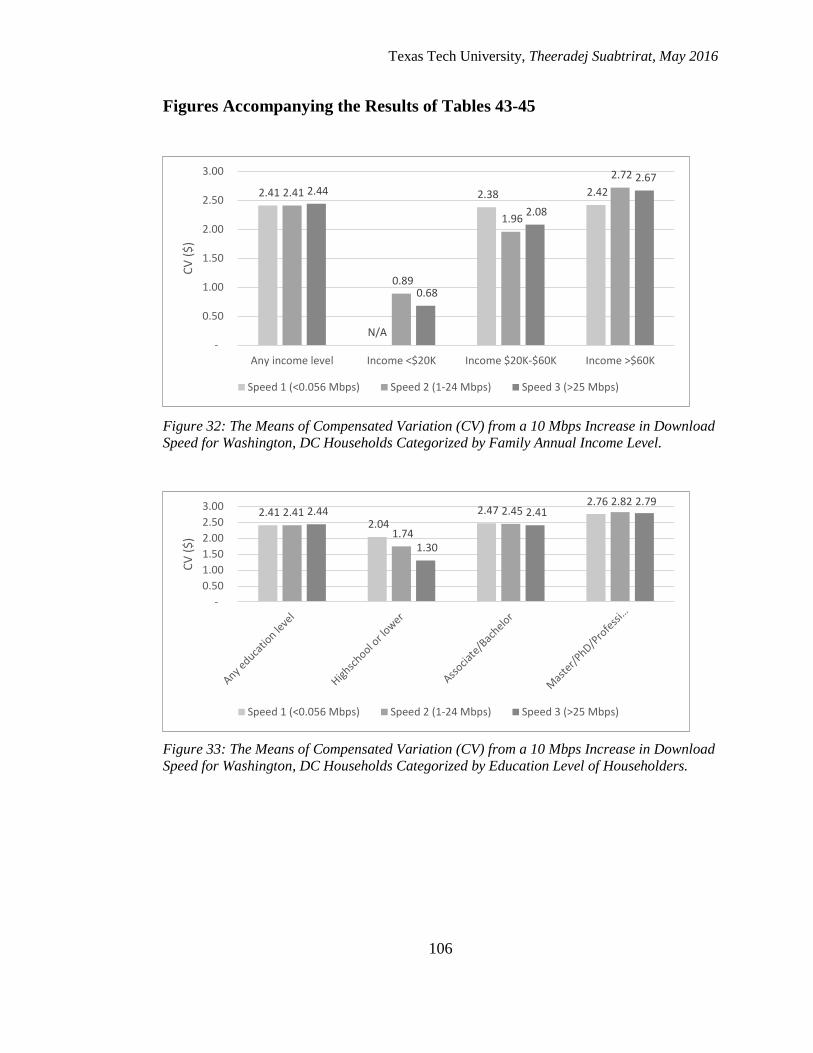
Texas Tech University, Theeradej Suabtrirat, May 2016
106
Figures Accompanying the Results of Tables 43-45
Figure 32: The Means of Compensated Variation (CV) from a 10 Mbps Increase in Download
Speed for Washington, DC Households Categorized by Family Annual Income Level.
Figure 33: The Means of Compensated Variation (CV) from a 10 Mbps Increase in Download
Speed for Washington, DC Households Categorized by Education Level of Householders.
2.41
N/A
2.38 2.42 2.41
0.89
1.96
2.72
2.44
0.68
2.08
2.67
-
0.50
1.00
1.50
2.00
2.50
3.00
Any income level Income <$20K Income $20K-$60K Income >$60K
CV
($
)
Speed 1 (<0.056 Mbps) Speed 2 (1-24 Mbps) Speed 3 (>25 Mbps)
2.41 2.04
2.47 2.76
2.41
1.74
2.45 2.82
2.44
1.30
2.41 2.79
-
0.50
1.00
1.50
2.00
2.50
3.00
CV
($
)
Speed 1 (<0.056 Mbps) Speed 2 (1-24 Mbps) Speed 3 (>25 Mbps)

Texas Tech University, Theeradej Suabtrirat, May 2016
107
Figure 34: The Means of Compensated Variation (CV) from a 10 Mbps Increase in Download
Speed for Washington, DC Households Categorized by Age Level of Householders.
Figure 35: Expected Adoption Increase from a 10 Mbps Increase in Download Speed for
Washington, DC Households Categorized by Levels of Family Annual Income, Education of
Householders, and Age of Householders.
2.41 2.54
2.42 2.35 2.41 2.49 2.41 2.30
2.44 2.61
2.42
2.07
-
0.50
1.00
1.50
2.00
2.50
3.00
Any age level Age 25-44 yrs Age 45-60 yrs Age 61-85 yrs
CV
($
)
Speed 1 (<0.056 Mbps) Speed 2 (1-24 Mbps) Speed 3 (>25 Mbps)
N/A
9.65%
17.54%
16.85%
39.43%
23.28%
22.90%
90.24%
90.90%
25.77%
0.00% 10.00% 20.00% 30.00% 40.00% 50.00% 60.00% 70.00% 80.00% 90.00% 100.00%
Income
Education
Age
Overall
Demographic Level 1 Demographic Level 2 Demographic Level 3

Texas Tech University, Theeradej Suabtrirat, May 2016
108
Figures Accompanying the Results of Tables 46-48
Figure 36: The Means of Compensated Variation (CV) from a 10 Mbps Increase in Download
Speed for New York City Households Categorized by Family Annual Income Level.
Figure 37: The Means of Compensated Variation (CV) from a 10 Mbps Increase in Download
Speed for New York City Households Categorized by Education Level of Householders.
5.19
4.29 4.80
5.71 5.18
2.82
4.66
6.00 5.42
3.06
4.70
5.96
-
1.00
2.00
3.00
4.00
5.00
6.00
7.00
Any income level Income <$20K Income $20K-$60K Income >$60K
CV
($
)
Speed 1 (<0.056 Mbps) Speed 2 (1-24 Mbps) Speed 3 (>25 Mbps)
5.19 4.77 5.33
5.95 5.18
4.10
5.51 6.15
5.42 4.48
5.52 6.19
- 1.00 2.00 3.00 4.00 5.00 6.00 7.00
CV
($
)
Speed 1 (<0.056 Mbps) Speed 2 (1-24 Mbps) Speed 3 (>25 Mbps)

Texas Tech University, Theeradej Suabtrirat, May 2016
109
Figure 38: The Means of Compensated Variation (CV) from a 10 Mbps Increase in Download
Speed for New York City Households Categorized by Age Level of Householders.
Figure 39: Expected Adoption Increase from a 10 Mbps Increase in Download Speed for New
York City Households Categorized by Levels of Family Annual Income, Education of
Householders, and Age of Householders.
5.19 5.08 5.24 5.15 5.18 5.50
5.20 4.64
5.42 5.74
5.43 4.88
-
1.00
2.00
3.00
4.00
5.00
6.00
7.00
Any age level Age 25-44 yrs Age 45-60 yrs Age 61-85 yrs
CV
($
)
Speed 1 (<0.056 Mbps) Speed 2 (1-24 Mbps) Speed 3 (>25 Mbps)
2.92%
18.58%
51.19%
40.37%
61.70%
40.19%
31.33%
98.00%
60.00%
18.27%
0.00% 20.00% 40.00% 60.00% 80.00% 100.00% 120.00%
Income
Education
Age
Overall
Demographic Level 1 Demographic Level 2 Demographic Level 3

Texas Tech University, Theeradej Suabtrirat, May 2016
110
CHAPTER V
POLICY IMPLICATIONS
This chapter focuses on policy implications from the econometric results of
this dissertation. Several solutions are proposed to encourage internet adoption and
improve digital literacy among certain groups of the U.S population who fall behind in
computer and internet use. The solutions are categorized into two groups: 1) solutions
supported by the results of this dissertation, and 2) solutions supported by the findings
of previous literature.
Solutions Supported by the Results of this Dissertation
This dissertation concludes that several factors increase the probability of
internet adoption: earning higher family income, attaining higher education levels,
having a residence in an urban area, and being employed. On the contrary, the factors
decreasing the probability of internet adoption include high prices of internet service,
older age, having disabilities that obstruct internet use, and lack of U.S. citizenship.
Solutions presented in this section aim at overcoming the following barriers: 1) digital
literacy, 2) cost, 3) irrelevance, 4) language, and 5) accessibility.
Overcoming Digital Literacy Barriers
Digital literacy is the ability to effectively use computers, communication
tools, and the Internet to find, evaluate, use, and create information (US Digital
Literacy 2015). This dissertation finds that households with low education attainment
tend to lag behind in digital literacy. Visser (2013, 106) finds that individuals lacking
digital literacy tend to be the ones who have less formal education, earn a low family
income, and live in underserved rural areas. The author further suggests that 1) public
libraries have been successful in offering digital literacy education for individuals with
the aforementioned characteristics; 2) successful training does not teach skills in
isolation but links them to certain specific outcomes (such as job seeking, financial
literacy, and legal issues research); and 3) formal classes and in-person assistance

Texas Tech University, Theeradej Suabtrirat, May 2016
111
should be given in combination so that individuals learn new skills in a formal class
and practice them in personal assisting sessions.
The FCC (2010, 174) finds that public libraries and community centers have
been providing digital literacy training to people with limited educational
opportunities. However, many public libraries and community centers report a lack of
computer equipment to serve their patrons. About 80% of libraries claimed that
patrons are often put on waiting lists and given a time limit of 30 or 60 minutes. Such
restrictions hinder patrons from using computers and the Internet at their leisure. The
FCC suggests supplying additional computer equipment to public libraries and
community centers to alleviate the problem.
Overcoming Cost Barriers
Householders who refuse to purchase home and mobile internet service
popularly cite “too expensive price” as their primary reason (NTIA 2014, 9).
Similarly, this dissertation concludes that 1) an increase in monthly price of internet
service tends to decrease the probability of home internet adoption; and 2) the demand
for home internet service is highly price-elastic. Reducing the monthly price of
internet connection should greatly boost internet adoption rates of low income
households.
The FCC plans to boost internet adoption among low-income households by
offering them a low-cost internet connection through the Lifeline Assistance and the
Link-Up America programs (FCC 2010, 168). These two programs are currently
providing phone services to low-income households at very affordable prices. For
example, the Lifeline Assistance by Verizon offers a mobile phone service for $24.74
per month and a landline service for $10.74 per month (Verizon 2015). The
implementation of these programs was highly successful; it boosted telephone
subscription of low-income households from 80% in 1984 to 89.7% in 2008. The FCC
suggests that the Congress should extend these two programs to home internet service
since they should be able to greatly boost home internet adoption among low-income
households, as they did with telephone service subscriptions.

Texas Tech University, Theeradej Suabtrirat, May 2016
112
Alternatively, the FCC suggests that a free internet connection could be made
available to American households through advertising-supported programs (FCC
2010, 172). Broadcast television (or free-to-air TV) is an example of successful
implementation of such program, providing American households with news,
information, shows, and programming. The National Broadband Plan suggests
licensing a frequency though an auction and requiring the licensees to offer a free or
very low cost internet service to households. However, the FCC is currently searching
for a successful business model for an advertising-supported internet connection.
Overcoming Irrelevance Barriers
Householders who refuse to use home and mobile internet cite “irrelevance to
daily lives” as their primary reason (FCC 2010, 174). The agency finds that such
householders have an average age of 61 years old. Similarly, this dissertation
concludes that the older age of householders are less likely to adopt home and mobile
internet services.
The FCC (2010, 179) suggests three ways to bring senior citizens into the
digital world: (1) show them how to use the Internet to discover tips for staying
healthy and locating nearby healthcare providers; 2) notify them about telemedicine
programs that enable health management at lower costs; and 3) introduce them to
social networking websites so that they can reconnect with their old friends and make
new friends without travelling from home. Previous studies find that senior citizens
are more likely to go online after seeing practical benefits of the Internet.
Overcoming Language Barriers
This dissertation concludes that there is an adoption gap among different races,
and that Hispanic households are found to fall behind other races in both home and
mobile internet adoption. This result is confirmed by previous literature such as
Livingston (2010, 7). The author finds that Hispanics fall behind Non-Hispanics in
terms of cell phone use (76% vs. 86%) and internet use (64% vs. 78%).
To fight against language barriers, the FCC (2010, 174) suggests that public
libraries and community centers should hire instructors with foreign language skills to

Texas Tech University, Theeradej Suabtrirat, May 2016
113
provide computer training to non-English speakers. Previous literature shows that the
lack of fluency with English and the scarcity of non-English websites are associated
with low levels of internet adoption. For example, only 20% of Hispanics who
participated in the FCC’s survey in Spanish replied that they have home internet. The
training provided in the learners’ native language (such as Spanish) or tailored for
learners who use English as their second language would effectively reduce cultural
and linguistic barriers between instructors and learners.
Overcoming Accessibility Barriers
People with disabilities are less likely to access the Internet since they face
many disability-related obstacles (FCC 2010, 181). This finding is similar to that of
this dissertation, which concludes that people with disabilities have lower probability
of home and mobile internet adoption.
The FCC makes three recommendations to make accessibility-supported
websites, hardware, and software available for people with disabilities. First, the
federal websites should be accessibly designed for people with various types of
disabilities. Second, the FCC plans to extend its Section 255 rules to require
manufacturers of end-user equipment to make their products compatible with
accessibility devices. For example, Apple has made its iOS to support hearing aid
devices through a Bluetooth connection (Apple Computer 2015). Samsung has created
the Eyecan+, an eye-ball tracking mouse that enables its users to click an object by
blinking their eyes (Wood 2014). Third, the Universal Service Fund should be
appropriated to projects with the following purposes: 1) projects to create assistive
technology that would enable individuals who are deaf or blind to use the Internet (up
to $10 million per year); and 2) projects to fund competitive awards for developers
who create innovative devices, software, and applications that promote internet
adoption (up to $10 million per year).

Texas Tech University, Theeradej Suabtrirat, May 2016
114
Solutions Supported by the Findings of Previous Literature
The following solutions are not directly supported by the results of this
dissertation but are relevant to the emphasis of this dissertation. These solutions are
strongly supported by the findings of previous literature for their ability to encourage
home and mobile internet adoption. Solutions presented in this section aim at: 1)
overcoming low internet adoption in low income areas, 2) overcoming insufficient
infrastructure in rural areas, and 3) expanding availability of information technology
employment.
Overcoming Low Internet Adoption in Low Income Areas
Despite prevalent availability of internet infrastructure, home and mobile
internet adoption tends to be too low in low income communities situated in urban and
suburban areas (Atkinson 2009, 3). Many ISPs choose not to recruit new customers in
such areas since the cost of doing so sometimes exceeds expected revenue. The cost
may involve digital literacy training and marketing expenses to explain the benefits of
the Internet to consumers. The author recommends that the National
Telecommunications and Information Administration (NTIA) should establish a
competition among ISPs and reward those that successfully recruit new customers. For
example, the winning ISP might be awarded $250 per new subscriber and a public
recognition at the White House. Cooperation from ISPs is very important since their
marketing campaign and customer service could persuade non-internet-using
households to purchase and start using internet service.
Overcoming Insufficient Infrastructure in Rural Areas
About 15 million Americans in rural areas do not have access to high-speed
internet service in their homes (Wheeler 2014). Moreover, about 41% of American
rural schools do not have access to high-speed internet. Modernizing the FCC’s E-rate
program will make high-speed internet available in rural communities. The FCC
proposes to increase the cap on American households’ contribution to the E-rate
program via telephone bill by 16 cents a month. The funding from a hike in the E-rate
will be spent on a one-time infrastructure investment needed by high-cost rural

Texas Tech University, Theeradej Suabtrirat, May 2016
115
libraries and schools. The FCC contends that an increase in E-rate is justified since the
E-Rate budget has not received an inflation adjustment for 13 years. Moreover, the
FCC has been remodeling the Universal Service Fund and the new Connect America
Fund to finance construction of high-speed internet networks in underserved rural
areas. These funds will invest about $20 billion over the next five years to create
internet connections with minimum download speeds of 10 Mbps for rural households.
Expanding Availability of Information Technology Employment
Information technology employment and telecommuting (work from home) are
found to be positively correlated with higher internet adoption rates (Tomer and Kane
2015, 7). Using a regression model, the authors show that internet adoption rates have
a positive relationship with: 1) the share of population living in urban area, 2) the
share of telecommuter (work-from-home workers), and 3) the share of workers in
service, technology, management, and education industries. These relationships are
statistically significant at 5% level. Therefore, creating telecommuting employment
and job opportunities in the aforementioned industries could be a good way to
encourage internet adoption since households will have an opportunity to earn income
by accumulating information technology skills.
Conclusion
This chapter relates the econometric results of this dissertation to the solutions
to encourage internet adoption and improve digital literacy of American households.
Solutions supported by the results of this dissertation suggests: 1) providing digital
literacy education to low education households; 2) reducing the monthly price of
internet service to low income households; 3) pointing out the benefits of the Internet
to senior citizens; 4) furnishing computer trainings in learners’ native language; and 5)
providing accessibility devices to people with disability. On the other hand, solutions
supported by the findings of previous literature suggest: 1) rewarding ISPs who
successfully recruit new customers in low income areas; 2) raising the fee of the E-rate

Texas Tech University, Theeradej Suabtrirat, May 2016
116
program and spending these funds on internet infrastructure in rural areas; and 3)
expanding availability of information technology employment. These solutions should
be able to effectively close the digital divide among non-internet using households.

Texas Tech University, Theeradej Suabtrirat, May 2016
117
BIBLIOGRAPHY
Ang, John. 2007. Discrete Choice Modeling with PROC MDC. The SouthEast SAS
Users Group Proceedings. http://analytics.ncsu.edu/sesug/2007/DM08.pdf
(accessed October 15, 2015).
Apple Computer. 2015. About Hearing Aid Compatibility Requirements for iPhone.
https://support.apple.com/en-us/HT202186 (accessed September 30, 2015).
Atkinson, Robert D. 2009. Policies to Increase Broadband Adoption at Home.
Information Technology and Innovation Foundation (November 2009).
http://www.itif.org/files/2009-demand-side-policies.pdf (accessed November
14, 2015).
Avila, Jonathan. 2014. Trends in Mobile Device Use by People with Disabilities.
Access IQ (March 2014).
http://www.accessiq.org/news/features/2014/03/trends-in-mobile-device-use-
by-people-with-disabilities (accessed March 8, 2016).
Beede, David N. 2014. Competition among U.S. Broadband Service Providers. Office
of the Chief Economist Issue Brief (December 2014).
http://esa.doc.gov/sites/default/files/competition-among-us-broadband-service-
providers.pdf (accessed September 24, 2015).
Cameron, Pravin K. and Colin A. Trivedi. 2010. Microeconometrics Using Stata:
Revised Edition. College Station, TX: Stata Press.
http://cameron.econ.ucdavis.edu/musbook/mus.html (accessed September 20,
2015).
Christensson, Per. 2009. Dial-up Definition. http://techterms.com/definition/dialup
(accessed September 14, 2015).
Computer and Communications Industry Association. 2013. Broadband Consumption
Survey. http://cdn.ccianet.org/wp-content/uploads/2013/10/Broadband-
Consumption-Survey-Exec-Summary.pdf (accessed February 15, 2016).
Consumer NZ. 2015. Internet Provider. https://www.consumer.org.nz/articles/internet-
providers (accessed September 24, 2015).
DSL Report. 2009. FCC: We're Halfway Done with National Broadband Plan. DSL
Report (September 2009). http://www.dslreports.com/shownews/FCC-Were-
Halfway-Done-With-National-Broadband-Plan-104715 (accessed April 20,
2015).

Texas Tech University, Theeradej Suabtrirat, May 2016
118
Duggan, Maeve, and Aaron Smith. 2013. Cell Internet Use 2013. Pew Research
Center (September 2013). http://www.pewinternet.org/2013/09/16/cell-
internet-use-2013/ (accessed September 27, 2015).
Dutz, Mark, Jonathan Orszag, and Robert Willig. 2009. The Substantial Consumer
Benefits of Broadband Connectivity for U.S. Households. Internet Innovation
Alliance (July 2009). http://internetinnovation.org/files/special-
reports/CONSUMER_BENEFITS_OF_BROADBAND.pdf (accessed
November 27, 2015).
Ericsson, Arthur D. Little, and Chalmers University of Technology. 2013.
Socioeconomic Effects of Broadband Speed. Ericsson (September 2013).
http://www.ericsson.com/res/thecompany/docs/corporate-
responsibility/2013/ericsson-broadband-final-071013.pdf (accessed February
13, 2016).
Federal Communication Commission. 2015. Household Broadband Guide.
http://www.fcc.gov/guides/household-broadband-guide (accessed January 18,
2015).
Federal Communication Commission. 2015b. Fourth International Broadband Data
Report. https://www.fcc.gov/document/fourth-international-broadband-data-
report-2015 (accessed January 25, 2015).
Federal Communication Commission. 2015c. Broadband Speed.
http://www.fcc.gov/encyclopedia/broadband-speed (accessed October 28,
2015).
Federal Communications Commission. 2010. National Broadband Plan: Connecting
America. https://transition.fcc.gov/national-broadband-plan/national-
broadband-plan.pdf (accessed September 14, 2015).
Federal Communications Commission. 2010b. Broadband Decisions: What Drives
Consumers to Switch–or Stick with–Their Broadband Internet Provider.
Federal Communications Commission Working Paper (December 2010).
https://apps.fcc.gov/edocs_public/attachmatch/DOC-303264A1.pdf (accessed
November 14, 2015).
File, Thom, and Camille Ryan. 2014. Computer and Internet Use in the United States
2013. American Community Survey Reports (November 2014).
http://www.census.gov/content/dam/Census/library/publications/2014/acs/acs-
28.pdf (accessed September 14, 2015).

Texas Tech University, Theeradej Suabtrirat, May 2016
119
Fox, Susannah, and Lee Rainie. 2014. The Web at 25 in the U.S. Pew Research Center
(February 2014). http://www.pewinternet.org/files/2014/02/PIP_25th-
anniversary-of-the-Web_0227141.pdf (accessed March 8, 2016).
Fung, Brian. 2015. Here’s How Data Caps Really Affect Your Internet Use,
According to Data. The Washington Post (July 14).
https://www.washingtonpost.com/news/the-switch/wp/2015/07/14/heres-how-
data-caps-really-affect-your-internet-use-according-to-data/ (accessed
September 24, 2015).
Greene, William H. 2008. Econometric Analysis. Upper Saddle River, NJ: Pearson
Prentice Hall.
Greenstein, Shane, and Ryan McDevitt. 2011. Evidence of a Modest Price Decline in
U.S. Broadband Services. Information Economics and Policy 23, no. 2: 200-
211. http://www.sciencedirect.com/science/article/pii/S0167624511000199
(accessed October 14, 2015).
Gurin, Joel. 2010. Internet Service: Would You Switch and Why?. Official FCC Blog.
https://www.fcc.gov/blog/internet-service-would-you-switch-and-why
(accessed October 28, 2015).
Hansen, Brianna. 2016. Mobile Productivity Survey. Wrike Inc.
https://www.wrike.com/blog/released-2016-mobile-productivity-report/
(accessed March 9, 2016).
Hill, R Carter, William E Griffiths, and Guay C Lim. 2008. Principles of
Econometrics. Hoboken, NJ: Wiley.
Hobbs, Joseph. 2008. World Regional Geography. Nelson Education.
International Labour Organization. 2001. The Digital Divide: Employment and
Development Implications. International Labour Review 140, no. 2: 113-117.
http://www.ilo.org/public/english/revue/download/pdf/intro012.pdf (accessed
March 6th, 2016).
Janke, James and David Trechter. 2014. Pierce County Broadband Internet Survey.
Survey Research Center Report of the University of Wisconsin at River Falls.
http://www.co.pierce.wi.us/Broadband%20survey%20report%20FINAL%20V
3-1.pdf (accessed January 6, 2016).
Jansen, Jim. 2010. Use of the Internet in Higher-Income Households. Pew Research
Center (November 2010). http://www.pewinternet.org/files/old-
media//Files/Reports/2010/PIP-Better-off-households-final.pdf (accessed
February 20, 2016).

Texas Tech University, Theeradej Suabtrirat, May 2016
120
Karlstrom, Anders and Edward Morey. 2003. Calculating the Exact Compensating
Variation in Logit and Nested-Logit Models with Income Effects: Theory,
Intuition, Implementation, and Application. Social Science Research Network
(May 2003). http://ssrn.com/abstract=562802 (accessed March 29, 2016).
Kehl, Danielle, Nick Russo, Robert Morgus, and Sarah Morris. 2014. The Cost of
Connectivity 2014. Open Technology Institute (October 2014).
https://www.newamerica.org/oti/the-cost-of-connectivity-2014/ (accessed
September 14, 2015).
Layton, Roslyn. 2014. The European Union’s Broadband Challenge. American
Enterprise Institute for Public Policy Research (February 2014).
https://www.aei.org/publication/the-european-unions-broadband-challenge/
(accessed September 14, 2015).
Lenhart, Amanda. 2015. Teen, Social Media and Technology Overview 2015. Pew
Research Center (April 2015).
http://www.pewinternet.org/files/2015/04/PI_TeensandTech_Update2015_040
9151.pdf (accessed March 15, 2016).
Lifetips. 2015. Five ISP Reliability Tips. http://isp.lifetips.com//cat/60536/isp-
reliability/index.html (accessed September 25, 2015).
Livingston, Gretchen. 2010. The Latino Digital Divide: the Native Born versus the
Foreign Born. Pew Research Center (July 2010).
http://www.pewhispanic.org/files/reports/123.pdf (accessed March 6, 2016).
Lopez, Mark Hugo, Ana Gonzalez-Barrera, and Eileen Patten. 2013. Closing the
Digital Divide: Latinos and Technology Adoption. Pew Hispanic Center
(March 2013). http://www.pewhispanic.org/2013/03/07/closing-the-digital-
divide-latinos-and-technology-adoption/ (accessed March 9, 2016.
MO Broadband Now. 2013. Survey on Residential Broadband.
http://mobroadbandnow.com/files/2013/06/Summary-Sheet-Residential-
Broadband-Survey-2013.pdf (accessed October 28, 2015).
McFadden, Daniel. 1995. Computing Willingness-to-Pay in Random Utility Models.
the University of California, Berkeley (December 1995).
http://citeseerx.ist.psu.edu/viewdoc/download?doi=10.1.1.18.1756&rep=rep1
&type=pdf (accessed March 30, 2016).
Murtagh, Rebecca. 2014. Mobile Now Exceeds PC: The Biggest Shift Since the
Internet Began. Search Engine Watch (July 2014).
http://searchenginewatch.com/sew/opinion/2353616/mobile-now-exceeds-pc-
the-biggest-shift-since-the-internet-began (accessed September 28, 2015).

Texas Tech University, Theeradej Suabtrirat, May 2016
121
National Telecommunications and Information Administration (NTIA) and Economics
and Statistics Administration (ESA). 2011. Exploring the Digital
Nation Computer and Internet Use at Home. U.S. Department of Commerce
(November 2011).
http://www.ntia.doc.gov/files/ntia/publications/exploring_the_digital_nation_c
omputer_and_internet_use_at_home_11092011.pdf (accessed September 3,
2015.
National Telecommunications and Information Administration (NTIA) and Economics
and Statistics Administration (ESA). 2013. Exploring the Digital Nation:
America's Emerging Online Experience. U.S. Department of Commerce (June
2013).
http://www.ntia.doc.gov/files/ntia/publications/exploring_the_digital_nation_-
_americas_emerging_online_experience.pdf (accessed September 15, 2015).
National Telecommunications and Information Administration (NTIA) and Economics
and Statistics Administration (ESA). 2014. Exploring the Digital Nation:
Embracing the Mobile Internet. U.S. Department of Commerce (October
2014).
http://www.ntia.doc.gov/files/ntia/publications/exploring_the_digital_nation_e
mbracing_the_mobile_internet_10162014.pdf (accessed September 17, 2015).
National Telecommunications and Information Administration (NTIA) and Federal
Communications Commission (FCC). 2014. Broadband Statistics Report:
Access to Broadband Technology by Speed. National Broadband Map (March
2015).
http://www.broadbandmap.gov/download/Technology%20by%20Speed.pdf
(accessed September 17, 2015).
National Telecommunications and Information Administration (NTIA). 2015. Internet
and Computer Use Studies and Data Files. http://www.ntia.doc.gov/data
(accessed September 15, 2015).
Nevo, Aviv. 2000. A Practitioner's Guide to Estimation of Random‐Coefficients Logit
Models of Demand. Journal of Economics & Management Strategy 9, no.4:
513-548.
http://faculty.wcas.northwestern.edu/~ane686/research/RAs_guide.pdf
(accessed March 29, 2016).
Nicholson, Walter, and Christopher Snyder. 2008. Microeconomic Theory: Basic
Principles and Extensions. Nelson Education.
Pinola, Melanie. 2013. How Do I Choose the Best Internet Service Provider?
http://lifehacker.com/how-do-i-choose-the-best-internet-service-provider-
480869389 (accessed March 6, 2015).

Texas Tech University, Theeradej Suabtrirat, May 2016
122
Price, Jason. 2015. Bundling Internet, TV and Phone: Is It Worth It?
http://www.biblemoneymatters.com/bundling-internet-tv-and-phone-is-it-
worth-it/ (accessed September 24, 2015).
Rosston, Gregory, Scott Savage, and Donald Waldman. 2011. Household Demand for
Broadband Internet Service. The Broadband.gov Task Force (February 2010).
http://www-siepr.stanford.edu/RePEc/sip/09-008.pdf (accessed February 13,
2015).
Saeedi, Maryam. 2015. Notes on Conditional Logit and Simulation. The Department
of Economics of the University of Minnesota.
http://www.econ.umn.edu/saeedi/numerical/logitexample.pdf (accessed
January 3, 2016).
SAS Institute Inc. 2014. SAS/ETS® 13.2 User’s Guide: The MDC Procedure. SAS
Institute Inc (August 2014).
https://support.sas.com/documentation/onlinedoc/ets/132/mdc.pdf (accessed
August 2014).
Scola, Nancy. 2014. If You Own a Smartphone, You Likely Live in or Near a City.
Next City (February 2014). https://nextcity.org/daily/entry/if-you-own-a-
smartphone-you-liekly-live-in-or-near-a-city (accessed March 8, 2015).
Segan, Sascha. 2015. How to Turn Your Phone into a Wi-Fi Hotspot. PC Magazine
(April 22). http://www.pcmag.com/article2/0,2817,2481374,00.asp (accessed
September 28, 2015.
Singleton, Micah. 2014. Data Caps Are a Long-Term Bet for Broadband Providers.
The Daily Dot (July 30). http://www.dailydot.com/technology/government-
finds-people-hate-data-caps (accessed September 14, 2015).
Singleton, Micah. 2015. The FCC Has Changed the Definition of Broadband. The
Verge (January 29). http://www.theverge.com/2015/1/29/7932653/fcc-
changed-definition-broadband-25mbps (accessed September 17, 2015).
Smith, Aaron. 2015. U.S. Smartphone Use in 2015. Pew Research Center (April
2015). http://www.pewinternet.org/2015/04/01/us-smartphone-use-in-2015/
(accessed September 26, 2015).
So, Ying and Warren F. Kuhfeld. 1995. Multinomial Logit Models. SAS User Group
International Conference Proceedings.
https://support.sas.com/techsup/technote/mr2010g.pdf (accessed September 5,
2015).

Texas Tech University, Theeradej Suabtrirat, May 2016
123
Tomer, Adie and Kane, Joseph. 2015. Broadband Adoption Rates and Gaps in U.S.
Metropolitan Areas. Brookings Metropolitan Policy Program (December
2015). http://www.brookings.edu/~/media/research/files/reports/2015/12/07-
broadband/broadband-tomer-kane-12315.pdf (accessed February 12, 2016).
UCLA Statistical Consulting Group. 2015. Stata Annotated Output: Logistic
Regression Analysis.
http://www.ats.ucla.edu/stat/stata/output/stata_logistic.htm (accessed
September 19, 2015).
U.S. Census Bureau. 2014. Computer and Internet Access in the United States 2012
Infographics. U.S. Census Bureau (February 2014).
http://www.census.gov/hhes/computer/files/2012/Computer_Use_Infographic_
FINAL.pdf (accessed April 5, 2016).
U.S. Digital Literacy. 2015. Digital and Media Literacy for Today’s Learners.
http://digitalliteracy.us (accessed October 10, 2015).
Verizon. 2015. Discounted Wireless through Lifeline Program Phone Service.
http://www.verizonwireless.com/wcms/consumer/explore/lifeline.html
(accessed September 29, 2015).
Visser, Marijke. 2013. Digital Literacy and Public Policy through the Library Lens.
Maine Policy Review 22, no. 1: 104-113.
http://digitalcommons.library.umaine.edu/cgi/viewcontent.cgi?article=1595&c
ontext=mpr (accessed November 14, 2015).
Wallsten, Scott, and Colleen Mallahan. 2010. Residential Broadband Competition in
the United States. Social Science Research Network (March 2010).
http://papers.ssrn.com/sol3/papers.cfm?abstract_id=1684236 (accessed
Febuary 3, 2016).
Wheeler, Tom. 2014. Closing the Digital Divide in Rural America.
https://www.fcc.gov/news-events/blog/2014/11/20/closing-digital-divide-rural-
america (accessed March 13, 2016).
Wood, Chris. 2014. Samsung Eye-Tracking Tech Lets Disabled Users Browse the
Web. GizMag (November 25). http://www.gizmag.com/samsung-eyecan-eye-
tracking-mouse/34927/ (accessed September 30, 2015).
Yu, Roger. 2012. Cable Companies Cap Data Use for Revenue. USA Today (October
1). http://www.usatoday.com/story/tech/2012/10/01/internet-data-
cap/1595683/ (accessed September 14, 2015).

Texas Tech University, Theeradej Suabtrirat, May 2016
124
Zickuhr, Kathryn, and Aaron Smith. 2012. Digital Differences. Pew Research Center
(April 2012). http://www.pewinternet.org/files/old-
media/Files/Reports/2012/PIP_Digital_differences_041312.pdf (accessed
February 29, 2016).