Copyright 2013 John Wiley & Sons, Inc.

Chapter 8 Supplement

Forecasting

8S-2

Forecasting Purposes and Methods

• Must forecast future to plan• An accurate estimate of demand is

crucial to the efficient operation of a system

• Not only demand can be forecasted– New technology– Economic conditions– Changes in lead time, scrap rates, and so on

8S-3

Primary Uses of Forecasting

1. To determine if sufficient demand exists

2. To determine long-term capacity needs

3. To determine midterm fluctuations in demand to avoid short-sighted decisions

4. To determine short-term fluctuations in demand for production planning, workforce scheduling, and materials planning

8S-4

Forecasting Methods

Figure 8S.1

8S-5

Qualitative Methods

• Life cycle

• Surveys

• Delphi

• Historical analogy

• Expert opinion

• Consumer panels

• Test marketing

8S-6

Quantitative Methods

• Causal– Input-output– Econometric– Box-Jenkins

• Time series analysis– Simple regression– Exponential smoothing– Moving average

8S-7

Choosing a Forecasting Method

1. Availability of representative data

2. Time and money limitations

3. Accuracy needed

8S-8

Time Series Analysis

• Time series is a set of values measured either at regular points in time or over sequential intervals of time

• Can be collected over short or long periods of time

8S-9

Components of Time Series

1. Trend T

2. Seasonal variation S

3. Cyclical variation C

4. Random variation R

8S-10

Common Trend Patterns

Figure 8S.2a

8S-11

Common Trend Patterns

Figure 8S.2b

8S-12

Common Trend Patterns

Figure 8S.2c

8S-13

Moving Averages

8S-14

Four-Period Moving Average of Intel’s Monthly Stock Closing Price

Figure 8S.3

8S-15

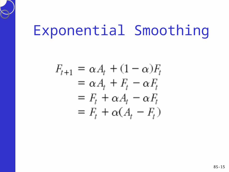
Exponential Smoothing

8S-16

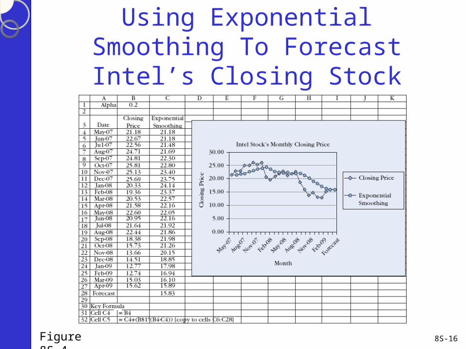
Using Exponential Smoothing To Forecast Intel’s Closing Stock Price

Figure 8S.4

8S-17

Simple Regression: The Linear Trend Multiplicative Model

Y = α + βX + ε

• Where:

• X = Independent variable

• Y = Dependent variable

• α and β are the parameter of the model

8S-18

Fitting Regression Line to Data

Figure 8S.5

8S-19

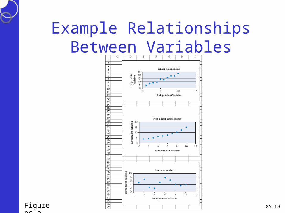
Example Relationships Between Variables

Figure 8S.8

8S-20

Least Squares Approach to Fitting Line to a Set of Data

Figure 8S.9

8S-21

Regression Analysis Assumptions

• The residuals are normally distributed

• The expected value of the residuals is zero

• The residuals are independent of one another

• The variance of the residuals is constant

8S-22

The Multiple Regression Model

• Simple regression uses one independent variable

• Using more than one independent variable is called multiple regression

• Form of the model is:

8S-23

Developing Regression Models

1. Identify candidate independent variables to include in the model

2. Transform the data

3. Select the variables to include in the model

4. Analyze the residuals