copyright © 2012 mcgraw-hill ryerson limited 11-1 powerpoint author: robert g. ducharme, macc, ca...
TRANSCRIPT
Copyright © 2012 McGraw-Hill Ryerson Limited
11-1
PowerPoint Author:
Robert G. Ducharme, MAcc, CAUniversity of Waterloo, School of Accounting and Finance
MANAGERIALACCOUNTINGNinth Canadian Edition GARRISON, CHESLEY, CARROLL, WEBB, LIBBY
MANAGERIALACCOUNTINGNinth Canadian Edition GARRISON, CHESLEY, CARROLL, WEBB, LIBBY
Reporting for Control
Chapter 11

11-2
Copyright © 2012 McGraw-Hill Ryerson Limited
Decentralization in Organizations
Benefits ofDecentralization Top management
freed to concentrateon strategy.
Top managementfreed to concentrate
on strategy.Lower-level managers
gain experience indecision-making.
Lower-level managersgain experience indecision-making. Decision-making
authority leads tojob satisfaction.
Decision-makingauthority leads tojob satisfaction.
Lower-level decisionsoften based on
better information.
Lower-level decisionsoften based on
better information.Lower level managers can respond quickly
to customers.
Lower level managers can respond quickly
to customers.LO 1

11-3
Copyright © 2012 McGraw-Hill Ryerson Limited
Decentralization in Organizations
Disadvantages ofDecentralization
Lower-level managersmay make decisionswithout seeing the
“big picture.”
Lower-level managersmay make decisionswithout seeing the
“big picture.”
May be a lack ofcoordination among
autonomousmanagers.
May be a lack ofcoordination among
autonomousmanagers.
Lower-level manager’sobjectives may not
be those of theorganization.
Lower-level manager’sobjectives may not
be those of theorganization. May be difficult to
spread innovative ideasin the organization.
May be difficult tospread innovative ideas
in the organization.
LO 1

11-4
Copyright © 2012 McGraw-Hill Ryerson Limited
Decentralization and Segment Reporting
A segmentsegment is any part or activity of an organization about which a manager
seeks cost, revenue, or profit data. A segment
can be . . .
Quick MartQuick Mart
An Individual Store
A Service Centre
A Sales Territory
LO 1
11-5
Copyright © 2012 McGraw-Hill Ryerson Limited
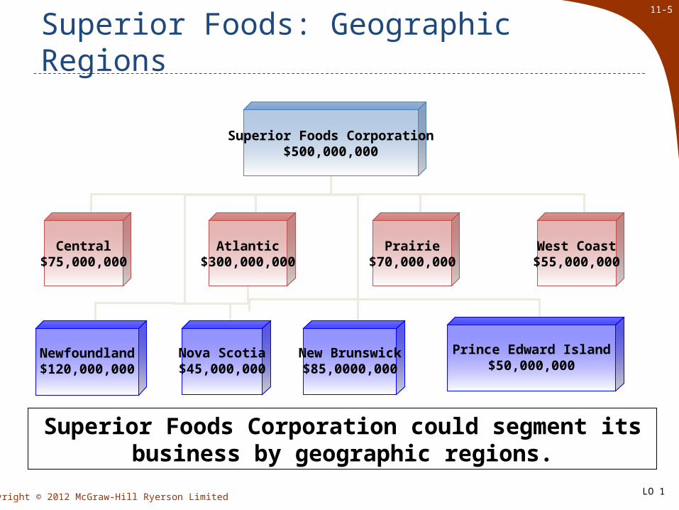
Superior Foods: Geographic Regions
Superior Foods Corporation could segment its business by geographic regions.
Superior Foods Corporation$500,000,000
Central$75,000,000
Atlantic$300,000,000
Prairie$70,000,000
West Coast$55,000,000
Nova Scotia$45,000,000
New Brunswick$85,0000,000
Prince Edward Island$50,000,000
Newfoundland$120,000,000
LO 1
11-6
Copyright © 2012 McGraw-Hill Ryerson Limited
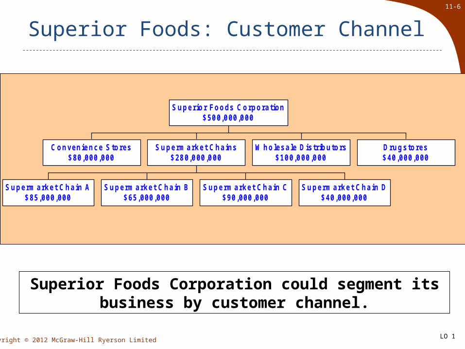
Superior Foods: Customer Channel
Convenience Stores$80,000,000
Supermarket Chain A$85,000,000
Supermarket Chain B$65,000,000
Supermarket Chain C$90,000,000
Supermarket Chain D$40,000,000
Supermarket Chains$280,000,000
W holesale Distributors$100,000,000
Drugstores$40,000,000
Superior Foods Corporation$500,000,000
Superior Foods Corporation could segment its business by customer channel.
LO 1
11-7
Copyright © 2012 McGraw-Hill Ryerson Limited
Keys to Segmented Income Statements
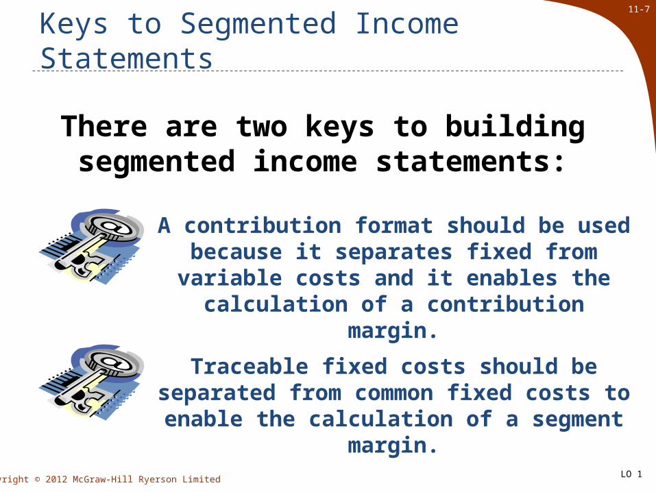
There are two keys to building segmented income statements:
A contribution format should be used because it separates fixed from variable costs
and it enables the calculation of a contribution margin.
Traceable fixed costs should be separated from common fixed costs to enable the
calculation of a segment margin.
LO 1
11-8
Copyright © 2012 McGraw-Hill Ryerson Limited
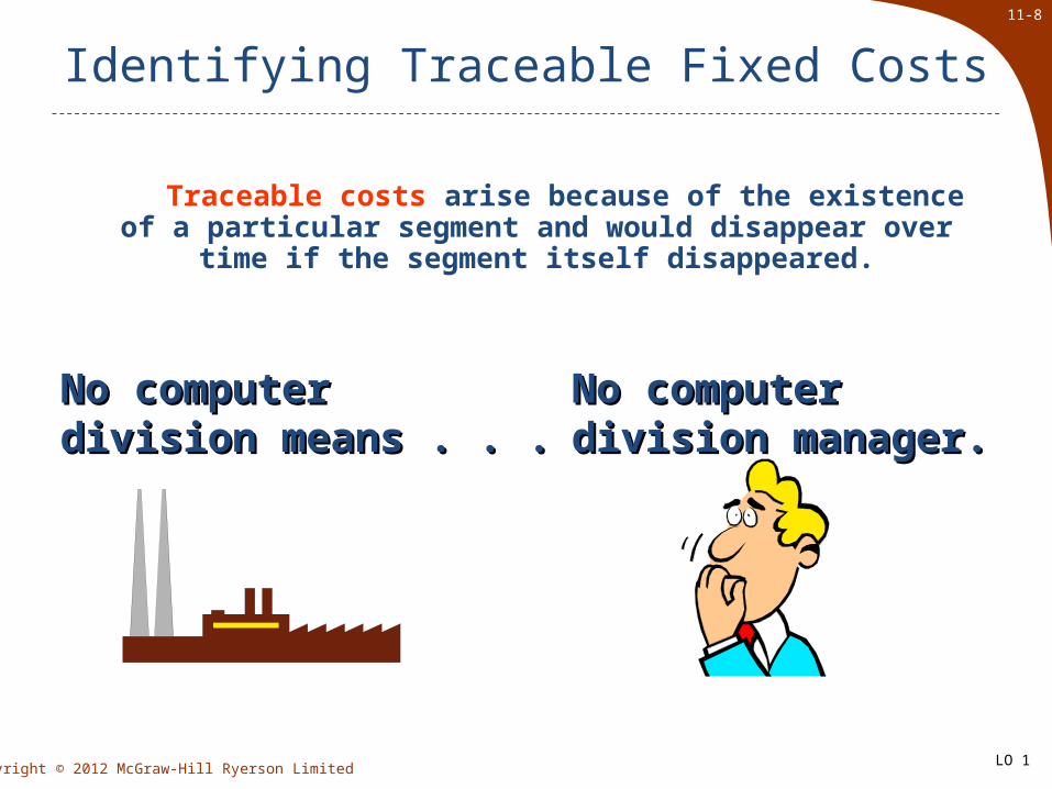
Identifying Traceable Fixed Costs
Traceable costs arise because of the existence of a particular segment and would disappear over
time if the segment itself disappeared.
No computer No computer division means . . .division means . . .
No computerNo computerdivision manager.division manager.
LO 1

11-9
Copyright © 2012 McGraw-Hill Ryerson Limited
Identifying Common Fixed Costs
Common costs arise because of the overall operation of the company and would not disappear if any particular segment were
eliminated.
No computer No computer division but . . .division but . . .
We still have aWe still have acompany president.company president.
LO 1
11-10
Copyright © 2012 McGraw-Hill Ryerson Limited
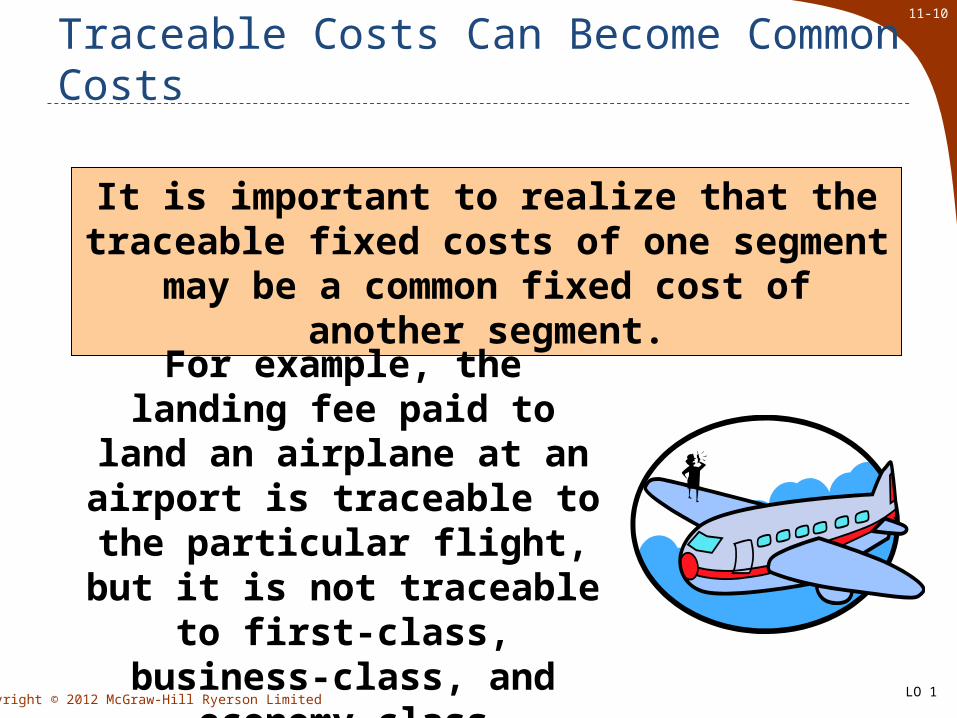
Traceable Costs Can Become Common Costs
It is important to realize that the traceable fixed costs of one segment may be a
common fixed cost of another segment.
For example, the landing fee paid to land an airplane at an
airport is traceable to the particular flight, but it is not
traceable to first-class, business-class, and
economy-class passengers.LO 1

11-11
Copyright © 2012 McGraw-Hill Ryerson Limited
Segment Margin
The segment margin, which is computed by subtracting the traceable fixed costs of a segment from its contribution margin, is the best gauge of
the long-run profitability of a segment.
TimeTime
Pro
fits
Pro
fits
LO 1
11-12
Copyright © 2012 McGraw-Hill Ryerson Limited
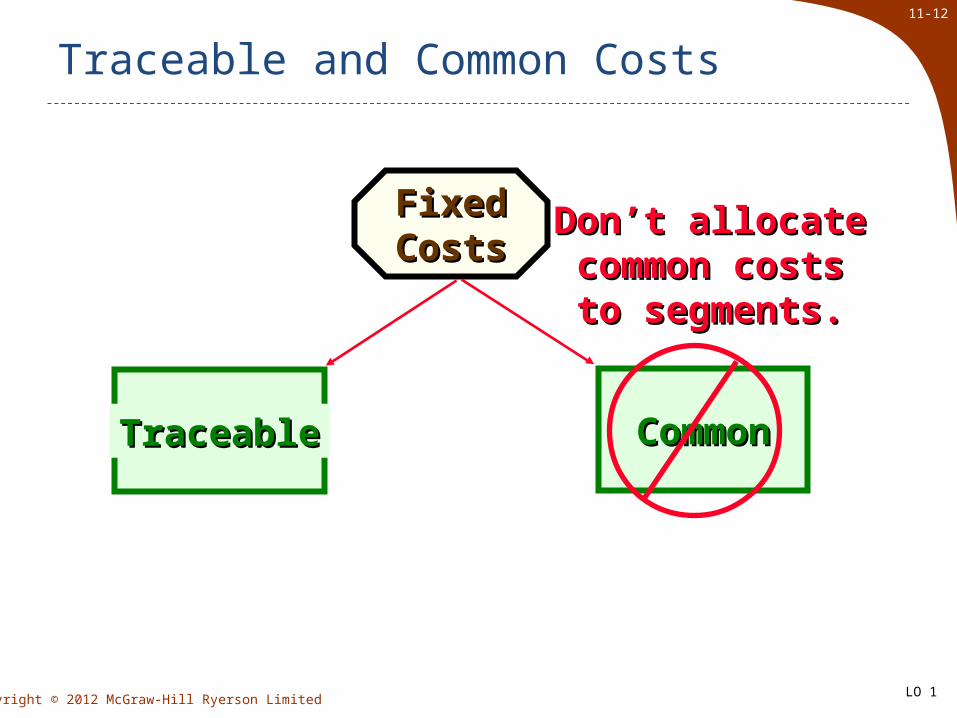
Traceable and Common Costs
FixedFixedCostsCosts
TraceableTraceable CommonCommon
Don’t allocateDon’t allocatecommon costs to common costs to
segments.segments.
LO 1

11-13
Copyright © 2012 McGraw-Hill Ryerson Limited
Activity-Based Costing
9-inch 12-inch 18-inch TotalWarehouse sq. ft. 1,000 4,000 5,000 10,000 Lease price per sq. ft. 4$ 4$ 4$ 4$ Total lease cost 4,000$ 16,000$ 20,000$ 40,000$
Pipe Products
Activity-based costing can help identify how costs shared by more than one segment are traceable to
individual segments. Assume that three products, 9-inch, 12-inch, and 18-inch pipe, share 10,000
square feet of warehousing space, which is leased at a price of $4 per square foot.
If the 9-inch, 12-inch, and 18-inch pipes occupy 1,000, 4,000, and 5,000 square feet, respectively, then ABC can be used to trace the warehousing costs to the
three products as shown.
LO 1
11-14
Copyright © 2012 McGraw-Hill Ryerson Limited
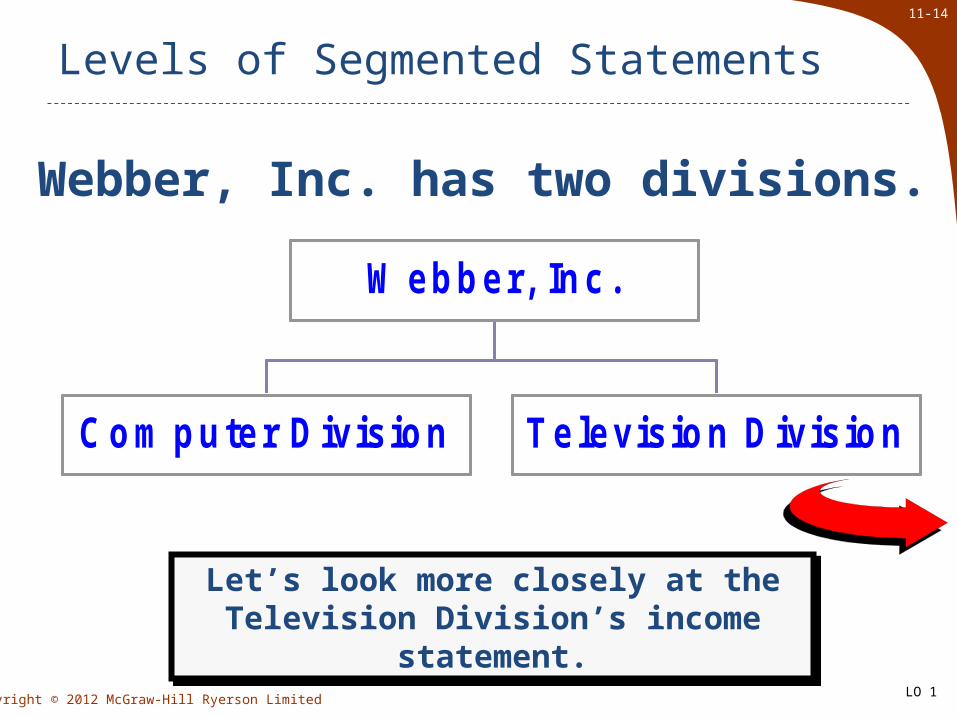
Levels of Segmented Statements
Let’s look more closely at the Television Division’s income statement.
Let’s look more closely at the Television Division’s income statement.
Webber, Inc. has two divisions.
Com puter Division Television Division
W ebber, Inc.
LO 1

11-15
Copyright © 2012 McGraw-Hill Ryerson Limited
Levels of Segmented Statements
Our approach to segment reporting uses the contribution format.
Income StatementContribution Margin Format
Television DivisionSales 300,000$ Variable COGS 120,000 Other variable costs 30,000 Total variable costs 150,000 Contribution margin 150,000 Traceable fixed costs 90,000 Division margin 60,000$
Cost of goodssold consists of
variable manufacturing
costs.
Cost of goodssold consists of
variable manufacturing
costs.
Fixed andvariable costsare listed in
separatesections.
Fixed andvariable costsare listed in
separatesections.
LO 1

11-16
Copyright © 2012 McGraw-Hill Ryerson Limited
Levels of Segmented Statements
Segment marginis Television’s
contributionto profits.
Segment marginis Television’s
contributionto profits.
Our approach to segment reporting uses the contribution format.
Income StatementContribution Margin Format
Television DivisionSales 300,000$ Variable COGS 120,000 Other variable costs 30,000 Total variable costs 150,000 Contribution margin 150,000 Traceable fixed costs 90,000 Division margin 60,000$
Contribution marginis computed by
taking sales minus variable costs.
Contribution marginis computed by
taking sales minus variable costs.
LO 1

11-17
Copyright © 2012 McGraw-Hill Ryerson Limited
Levels of Segmented Statements
Income StatementCompany Television Computer
Sales 500,000$ 300,000$ 200,000$ Variable costs 230,000 150,000 80,000 CM 270,000 150,000 120,000 Traceable FC 170,000 90,000 80,000 Division margin 100,000 60,000$ 40,000$
Common costsNet operating income
LO 1

11-18
Copyright © 2012 McGraw-Hill Ryerson Limited
Levels of Segmented Statements
Income StatementCompany Television Computer
Sales 500,000$ 300,000$ 200,000$ Variable costs 230,000 150,000 80,000 CM 270,000 150,000 120,000 Traceable FC 170,000 90,000 80,000 Division margin 100,000 60,000$ 40,000$
Common costs 25,000 Net operating income 75,000$
Common costs should not be allocated to the
divisions. These costs would remain even if one
of the divisions were eliminated.
Common costs should not be allocated to the
divisions. These costs would remain even if one
of the divisions were eliminated.
LO 1

11-19
Copyright © 2012 McGraw-Hill Ryerson Limited
Traceable Costs Can Become Common Costs
As previously mentioned, fixed costs that are traceable to one segment can become common if the company is divided into
smaller smaller segments.
Let’s see how this works using the Webber, Inc.
example!
LO 1

11-20
Copyright © 2012 McGraw-Hill Ryerson Limited
Traceable Costs Can Become Common Costs
ProductProductLinesLines
Webber’s Television Division
Regular Big Screen
TelevisionDivision
LO 1
11-21
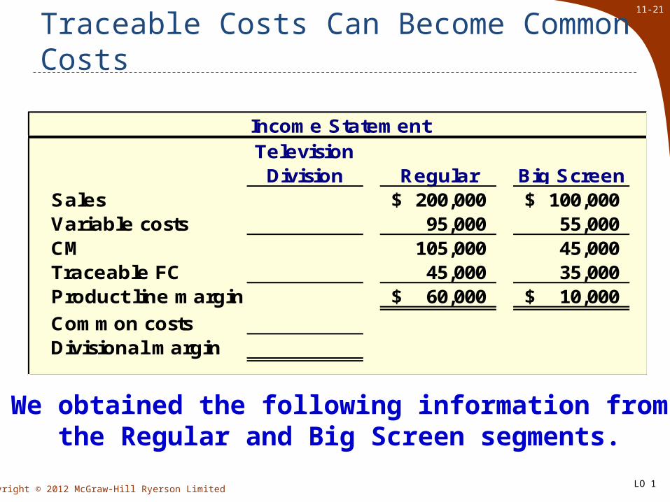
Copyright © 2012 McGraw-Hill Ryerson Limited
Traceable Costs Can Become Common Costs
We obtained the following information fromthe Regular and Big Screen segments.
Income StatementTelevision
Division Regular Big ScreenSales 200,000$ 100,000$ Variable costs 95,000 55,000 CM 105,000 45,000 Traceable FC 45,000 35,000 Product line margin 60,000$ 10,000$
Common costsDivisional margin
LO 1

11-22
Copyright © 2012 McGraw-Hill Ryerson Limited
Income StatementTelevision
Division Regular Big ScreenSales 300,000$ 200,000$ 100,000$ Variable costs 150,000 95,000 55,000 CM 150,000 105,000 45,000 Traceable FC 80,000 45,000 35,000 Product line margin 70,000 60,000$ 10,000$
Common costs 10,000 Divisional margin 60,000$
Traceable Costs Can Become Common Costs
Fixed costs directly tracedto the Television Division
$80,000 + $10,000 = $90,000
Fixed costs directly tracedto the Television Division
$80,000 + $10,000 = $90,000
LO 1
11-23
Copyright © 2012 McGraw-Hill Ryerson Limited
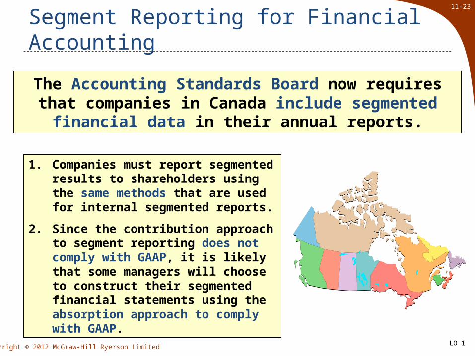
Segment Reporting for Financial Accounting
The Accounting Standards Board now requires that companies in Canada include segmented financial data in
their annual reports.
1. Companies must report segmented results to shareholders using the same methods that are used for internal segmented reports.
2. Since the contribution approach to segment reporting does not comply with GAAP, it is likely that some managers will choose to construct their segmented financial statements using the absorption approach to comply with GAAP.
LO 1

11-24
Copyright © 2012 McGraw-Hill Ryerson Limited
Some ProblemsSome Problems
Omission of some
costs in the
assignment process.
Use of inappropriate
methods for allocating
costs among segments.
Assignment to segments
of costs that are
really common costs of
the entire organization.
LO 1
Hindrances to Proper Cost Assignment

11-25
Copyright © 2012 McGraw-Hill Ryerson Limited
Omission of Costs
Costs assigned to a segment should include all costs attributable to that segment from the
company’s entire value chainvalue chain.
Product Customer R&D Design Manufacturing Marketing Distribution Service
Business FunctionsBusiness FunctionsMaking Up TheMaking Up The
Value ChainValue Chain
LO 1

11-26
Copyright © 2012 McGraw-Hill Ryerson Limited
Inappropriate Methods of Allocating Costs Among Segments
Segment1
Segment3
Segment4
Inappropriateallocation base
Segment2
Failure to tracecosts directly
LO 1
11-27
Copyright © 2012 McGraw-Hill Ryerson Limited
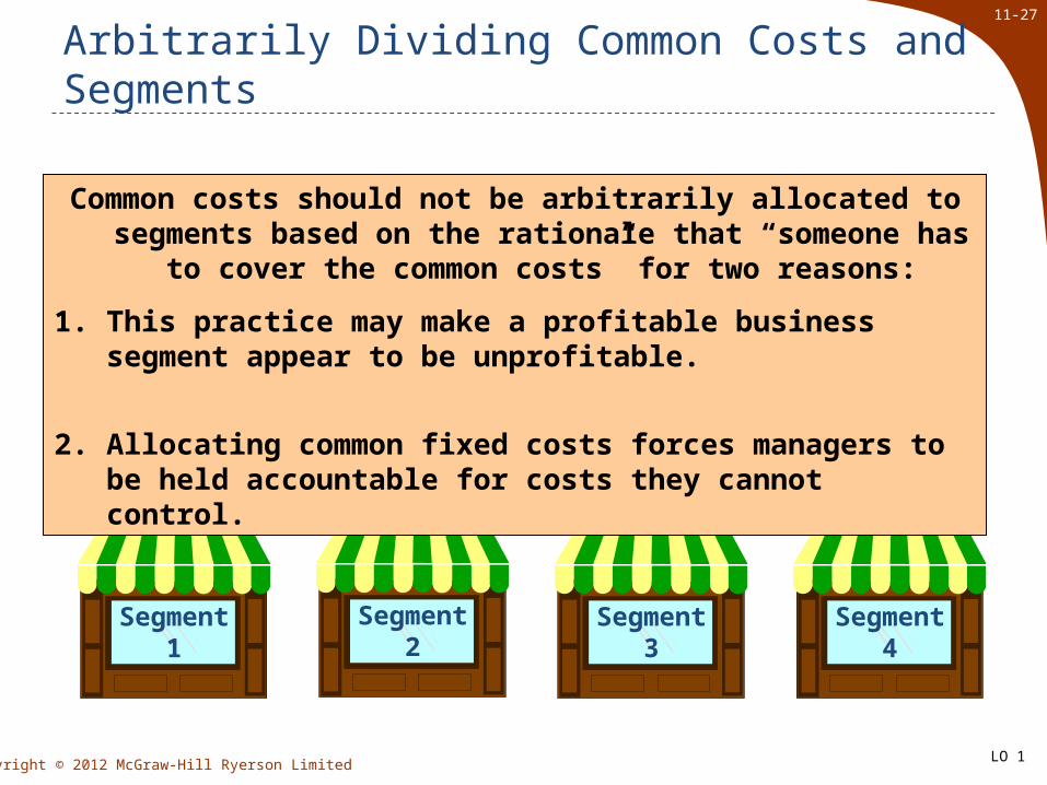
Arbitrarily Dividing Common Costs and Segments
Segment1
Segment3
Segment4
Segment2
Common costs should not be arbitrarily allocated to segments based on the rationale that “someone has to cover the
common costs” for two reasons:
1. This practice may make a profitable business segment appear to be unprofitable.
2. Allocating common fixed costs forces managers to be held accountable for costs they cannot control.
LO 1

11-28
Copyright © 2012 McGraw-Hill Ryerson Limited
Income StatementHaglund's Lakeshore Bar Restaurant
Sales 800,000$ 100,000$ 700,000$ Variable costs 310,000 60,000 250,000 CM 490,000 40,000 450,000 Traceable FC 246,000 26,000 220,000 Segment margin 244,000 14,000$ 230,000$
Common costs 200,000 Profit 44,000$
Quick Check
Assume that Hagland's Lakeshore prepared its segmented income statement as shown.
LO 1

11-29
Copyright © 2012 McGraw-Hill Ryerson Limited
Quick Check
How much of the common fixed cost of $200,000 can be avoided by eliminating the bar?a. None of it.b. Some of it.c. All of it.
LO 1

11-30
Copyright © 2012 McGraw-Hill Ryerson Limited
Quick Check
How much of the common fixed cost of $200,000 can be avoided by eliminating the bar?a. None of it.b. Some of it.c. All of it.
A common fixed cost cannot be eliminated by dropping one
of the segments.
LO 1

11-31
Copyright © 2012 McGraw-Hill Ryerson Limited
Quick Check
Suppose square feet is used as the basis for allocating the common fixed cost of $200,000. How much would be allocated to the bar if the bar occupies 1,000 square feet and the restaurant 9,000 square feet?a. $20,000b. $30,000c. $40,000d. $50,000
LO 1

11-32
Copyright © 2012 McGraw-Hill Ryerson Limited
Quick Check
Suppose square feet is used as the basis for allocating the common fixed cost of $200,000. How much would be allocated to the bar if the bar occupies 1,000 square feet and the restaurant 9,000 square feet?a. $20,000b. $30,000c. $40,000d. $50,000
The bar would be allocated 1/10 of the cost
or $20,000.
LO 1

11-33
Copyright © 2012 McGraw-Hill Ryerson Limited
Quick Check
If Hagland's allocates its common costs to the bar and the restaurant, what would be the reported profit of
each segment?
LO 1

11-34
Copyright © 2012 McGraw-Hill Ryerson Limited
Income StatementHaglund's Lakeshore Bar Restaurant
Sales 800,000$ 100,000$ 700,000$ Variable costs 310,000 60,000 250,000 CM 490,000 40,000 450,000 Traceable FC 246,000 26,000 220,000 Segment margin 244,000 14,000 230,000 Common costs 200,000 20,000 180,000 Profit 44,000$ (6,000)$ 50,000$
Allocations of Common Costs
Hurray, now everything adds up!!!
LO 1
11-35
Copyright © 2012 McGraw-Hill Ryerson Limited
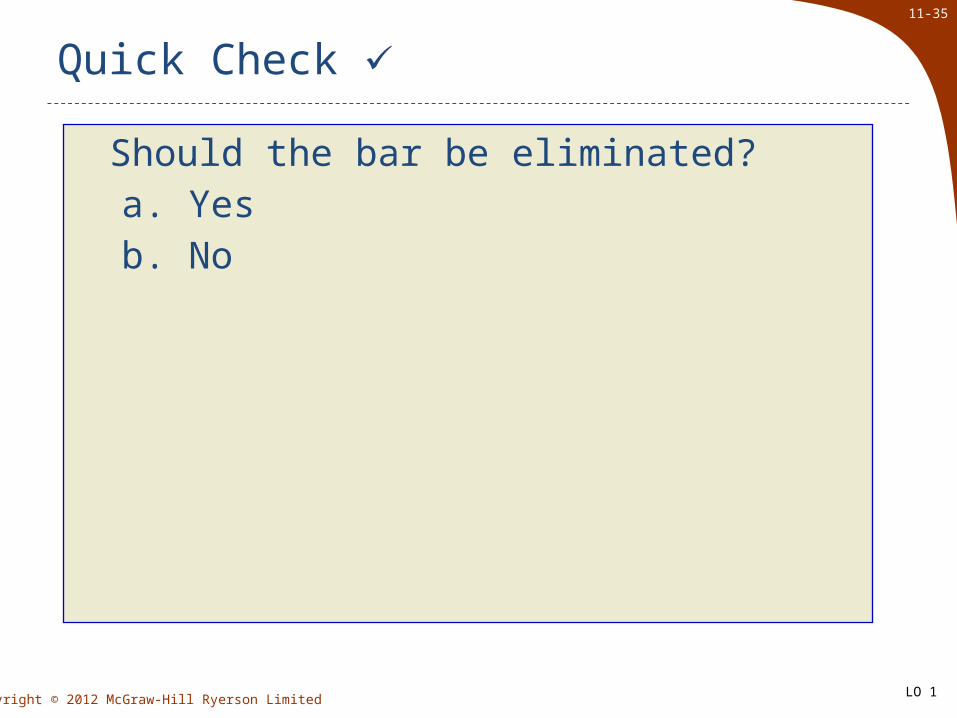
Quick Check
Should the bar be eliminated?a. Yesb. No
LO 1

11-36
Copyright © 2012 McGraw-Hill Ryerson Limited
Should the bar be eliminated?a. Yesb. No
Quick Check
Income StatementHaglund's Lakeshore Bar Restaurant
Sales 700,000$ 700,000$ Variable costs 250,000 250,000 CM 450,000 450,000 Traceable FC 220,000 220,000 Segment margin 230,000 230,000 Common costs 200,000 200,000 Profit 30,000$ 30,000$
The profit was $44,000 before eliminating the bar. If we eliminate
the bar, profit drops to $30,000!
LO 1

11-37
Copyright © 2012 McGraw-Hill Ryerson Limited
Cost, Profit, and Investments centres
Responsibilitycentre
Responsibilitycentre
CostcentreCost
centreProfitcentreProfitcentre
Investmentcentre
Investmentcentre
Cost, profit,and investmentcentres are allknown asresponsibilitycentres.
LO 2
11-38
Copyright © 2012 McGraw-Hill Ryerson Limited
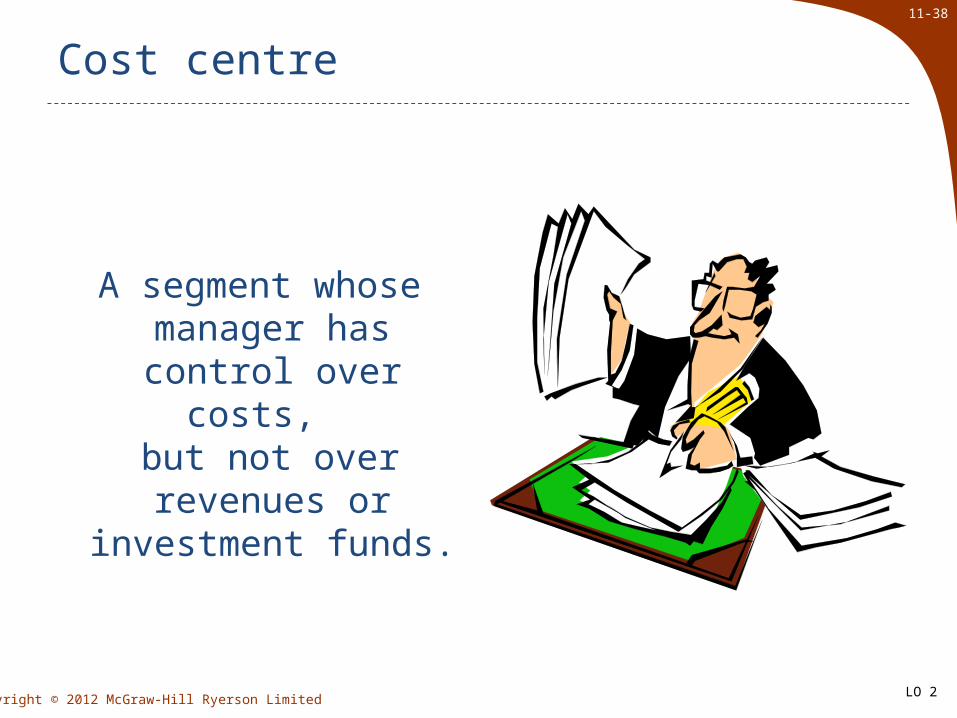
Cost centre
A segment whose manager has control
over costs, but not over revenues
or investment funds.
LO 2

11-39
Copyright © 2012 McGraw-Hill Ryerson Limited
Profit centre
A segment whose manager has control over both costs and
revenues, but no control over
investment funds.
Revenues
Sales
Interest
Other
Costs
Mfg. costs
Commissions
Salaries
Other
LO 2

11-40
Copyright © 2012 McGraw-Hill Ryerson Limited
Investment centre
A segment whose manager has control
over costs, revenues, and investments in
operating assets.
Corporate Headquarters
LO 2

11-41
Copyright © 2012 McGraw-Hill Ryerson Limited
Responsibility centres
Salty SnacksProduct M anger
Bottling P lantM anager
W arehouseM anager
DistributionM anager
BeveragesProduct M anager
ConfectionsProduct M anager
OperationsVice President
FinanceChief FInancial Officer
LegalGeneral Counsel
PersonnelVice President
Superior Foods CorporationCorporate Headquarters
President and CEO
Cost Centres
Investment Centres
Superior Foods Corporation provides an example of the various kinds of responsibility centres that exist in an
organization.LO 2
11-42
Copyright © 2012 McGraw-Hill Ryerson Limited
Responsibility centres
Salty SnacksProduct M anger
Bottling P lantM anager
W arehouseM anager
DistributionM anager
BeveragesProduct M anager
ConfectionsProduct M anager
OperationsVice President
FinanceChief FInancial Officer
LegalGeneral Counsel
PersonnelVice President
Superior Foods CorporationCorporate Headquarters
President and CEO
Superior Foods Corporation provides an example of the various kinds of responsibility centres that exist in an
organization.
Profit Centres
LO 2

11-43
Copyright © 2012 McGraw-Hill Ryerson Limited
Responsibility centres
Salty SnacksProduct M anger
Bottling P lantM anager
W arehouseM anager
DistributionM anager
BeveragesProduct M anager
ConfectionsProduct M anager
OperationsVice President
FinanceChief FInancial Officer
LegalGeneral Counsel
PersonnelVice President
Superior Foods CorporationCorporate Headquarters
President and CEO
Cost Centres
Superior Foods Corporation provides an example of the various kinds of responsibility centres that exist in an
organization.LO 2

11-44
Copyright © 2012 McGraw-Hill Ryerson Limited
Key Concepts/Definitions
A transfer price is the price charged when one segment of a company provides goods or
services to another segment of the company.
The fundamental objective in setting transfer prices is to
motivate managers to act in the best interests of the overall
company.
LO 3

11-45
Copyright © 2012 McGraw-Hill Ryerson Limited
Three Primary Approaches
There are three primary approaches to setting
transfer prices:
1. Negotiated transfer prices;
2. Transfers at the cost to the selling division; and
3. Transfers at market price.
LO 3
11-46
Copyright © 2012 McGraw-Hill Ryerson Limited
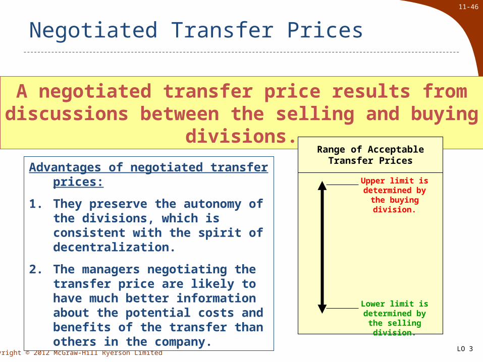
Negotiated Transfer Prices
A negotiated transfer price results from discussions between the selling and buying divisions.
Advantages of negotiated transfer prices:
1. They preserve the autonomy of the divisions, which is consistent with the spirit of decentralization.
2. The managers negotiating the transfer price are likely to have much better information about the potential costs and benefits of the transfer than others in the company.
Upper limit is determined by the buying division.
Lower limit is determined by the selling division.
Range of Acceptable Transfer Prices
LO 3
11-47
Copyright © 2012 McGraw-Hill Ryerson Limited
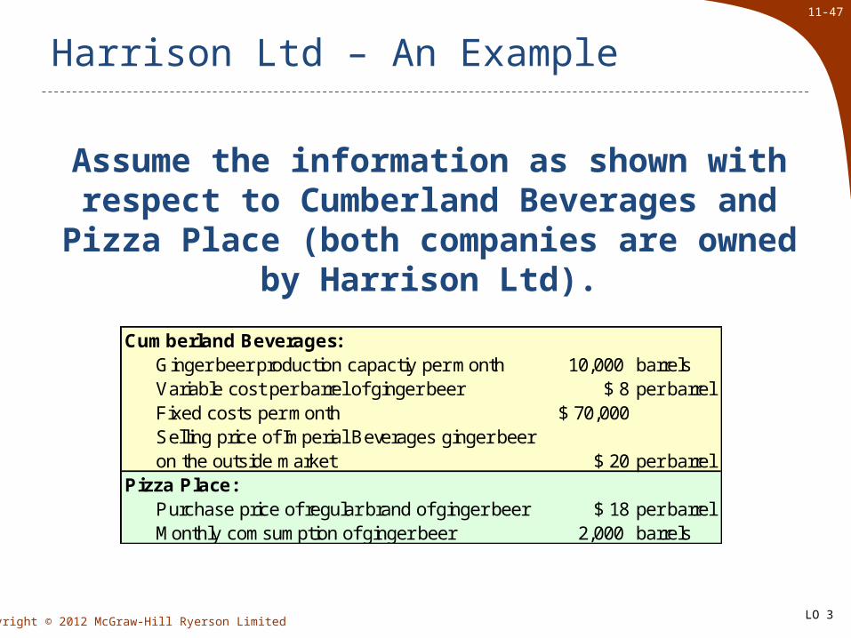
Harrison Ltd – An Example
Cumberland Beverages:Ginger beer production capactiy per month 10,000 barrelsVariable cost per barrel of ginger beer $ 8 per barrelFixed costs per month $ 70,000Selling price of Imperial Beverages ginger beer on the outside market $ 20 per barrel
Pizza Place:Purchase price of regular brand of ginger beer $ 18 per barrelMonthly comsumption of ginger beer 2,000 barrels
Assume the information as shown with respect to Cumberland Beverages and Pizza Place
(both companies are owned by Harrison Ltd).
LO 3

11-48
Copyright © 2012 McGraw-Hill Ryerson Limited
Harrison Ltd – An Example
The selling division’s (Cumberland Beverages) lowest acceptable transfer price is calculated as:
Variable cost Total contribution margin on lost salesper unit Number of units transferred
Transfer Price +
Transfer Price Cost of buying from outside supplier
The buying division’s (Pizza Place) highest acceptable transfer price is calculated as:
Let’s calculate the lowest and highest acceptable transfer prices under three scenarios.
Transfer Price Profit to be earned per unit sold (not including the transfer price)
If an outside supplier does not exist, the highest acceptable transfer price is calculated as:
LO 3

11-49
Copyright © 2012 McGraw-Hill Ryerson Limited
Harrison Ltd – An Example
If Cumberland Beverages has sufficient idle capacity (3,000 barrels) to satisfy Pizza Place’s demands (2,000 barrels), without sacrificing sales to other
customers, then the lowest and highest possible transfer prices are computed as follows:
$02,000
= $8Transfer Price +$8
Selling division’s lowest possible transfer price:
Transfer Price Cost of buying from outside supplier = $18Buying division’s highest possible transfer price:
Therefore, the range of acceptable transfer price is $8 – $18.
LO 3

11-50
Copyright © 2012 McGraw-Hill Ryerson Limited
Harrison Ltd – An Example
If Cumberland Beverages has no idle capacity (0 barrels) and must sacrifice other customer orders (2,000 barrels) to meet Pizza Place’s demands (2,000 barrels), then the lowest and highest possible transfer prices are computed
as follows:
( $20 - $8) × 2,0002,000
= $20Transfer Price +$8
Selling division’s lowest possible transfer price:
Transfer Price Cost of buying from outside supplier = $18Buying division’s highest possible transfer price:
Therefore, there is no range of acceptable transfer prices.
LO 3
11-51
Copyright © 2012 McGraw-Hill Ryerson Limited
Harrison Ltd – An Example
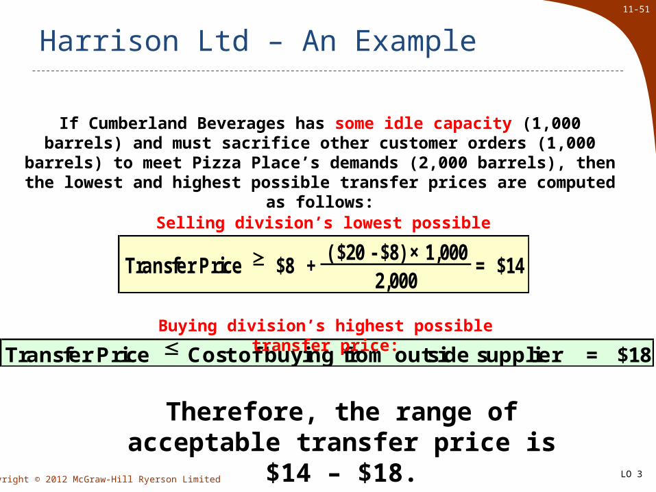
If Cumberland Beverages has some idle capacity (1,000 barrels) and must sacrifice other customer orders (1,000 barrels) to meet Pizza Place’s
demands (2,000 barrels), then the lowest and highest possible transfer prices are computed as follows:
Transfer Price Cost of buying from outside supplier = $18Buying division’s highest possible transfer price:
Therefore, the range of acceptable transfer price is $14 – $18.
Selling division’s lowest possible transfer price:
( $20 - $8) × 1,0002,000
= $14Transfer Price +$8
LO 3
11-52
Copyright © 2012 McGraw-Hill Ryerson Limited
Evaluation of Negotiated Transfer Prices
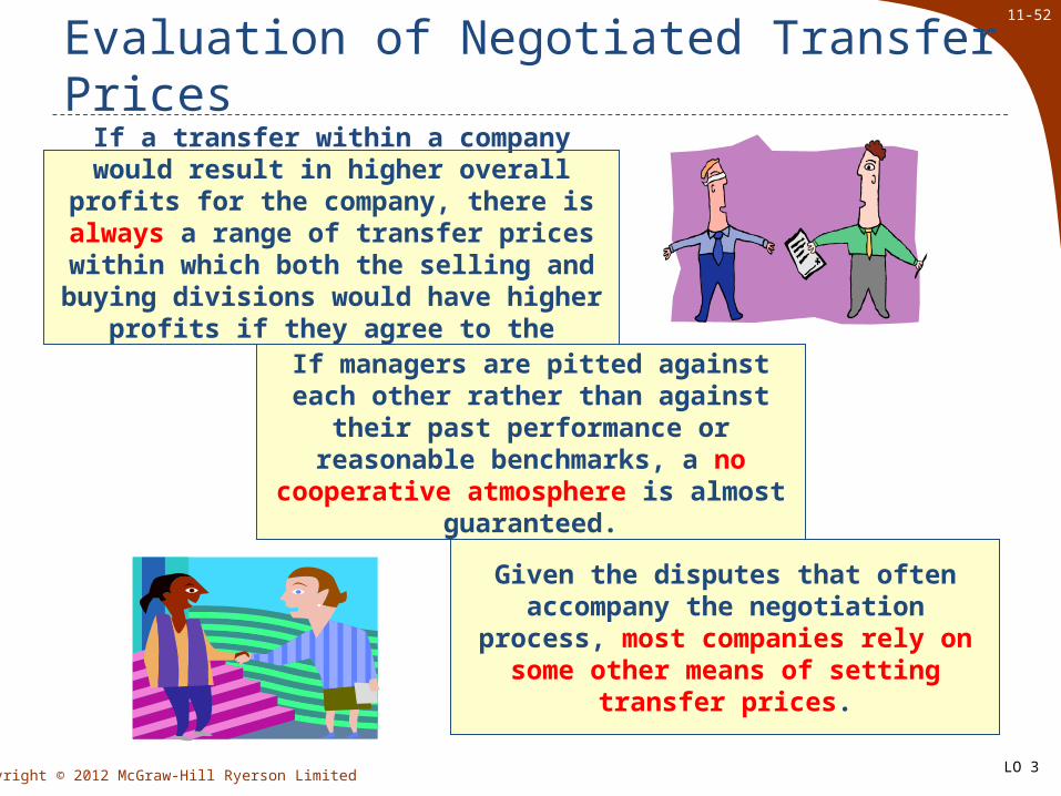
If a transfer within a company would result in higher overall profits for the company, there is always a range of transfer prices within which both the selling and buying
divisions would have higher profits if they agree to the transfer.
If managers are pitted against each other rather than against their past
performance or reasonable benchmarks, a no cooperative atmosphere is almost
guaranteed.
Given the disputes that often accompany the negotiation process, most companies
rely on some other means of setting transfer prices.
LO 3
11-53
Copyright © 2012 McGraw-Hill Ryerson Limited
Transfers at the Cost to the Selling Division
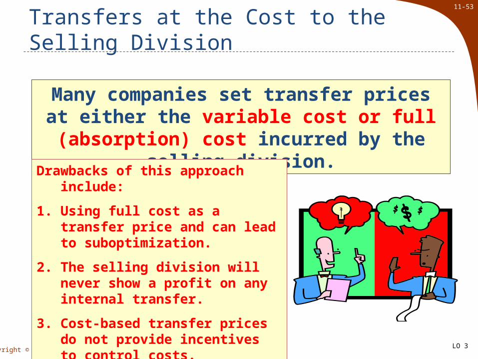
Many companies set transfer prices at either the variable cost or full (absorption) cost
incurred by the selling division.
Drawbacks of this approach include:
1. Using full cost as a transfer price and can lead to suboptimization.
2. The selling division will never show a profit on any internal transfer.
3. Cost-based transfer prices do not provide incentives to control costs.
LO 3

11-54
Copyright © 2012 McGraw-Hill Ryerson Limited
Transfers at Market Price
A market price (i.e., the price charged for an item on the open market) is often regarded as
the best approach to the transfer pricing problem.
1. A market price approach works best when the product or service is sold in its present form to outside customers and the selling division has no idle capacity.
2. A market price approach does not work well when the selling division has idle capacity.
LO 3

11-55
Copyright © 2012 McGraw-Hill Ryerson Limited
Divisional Autonomy and Sub optimization
The principles of decentralization suggest that companies should
grant managers autonomy to set transfer prices and to decide whether to sell internally or externally,
even if this may occasionally result in
suboptimal decisions.
This way top management allows subordinates to
control their own destiny.LO 3
11-56
Copyright © 2012 McGraw-Hill Ryerson Limited
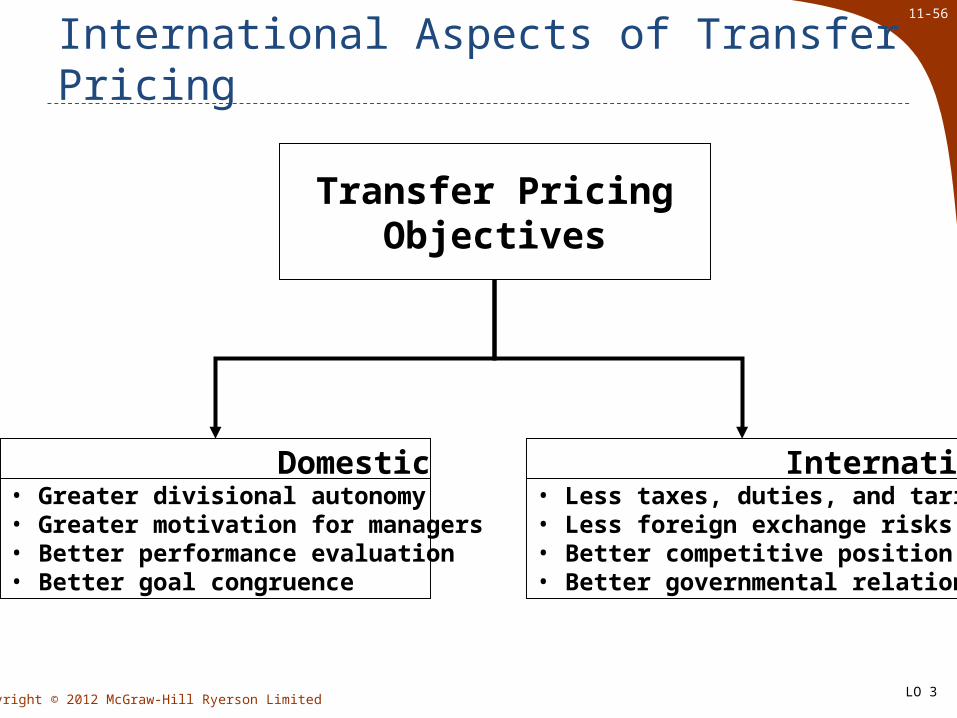
International Aspects of Transfer Pricing
Transfer Pricing Objectives
Domestic• Greater divisional autonomy• Greater motivation for managers• Better performance evaluation• Better goal congruence
International• Less taxes, duties, and tariffs• Less foreign exchange risks• Better competitive position• Better governmental relations
LO 3
11-57
Copyright © 2012 McGraw-Hill Ryerson Limited
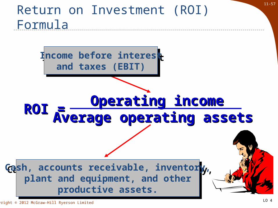
Return on Investment (ROI) Formula
ROI = ROI = Operating incomeOperating incomeAverage operating assets Average operating assets
Cash, accounts receivable, inventory,plant and equipment, and other
productive assets.
Cash, accounts receivable, inventory,plant and equipment, and other
productive assets.
Income before interestand taxes (EBIT)
Income before interestand taxes (EBIT)
LO 4

11-58
Copyright © 2012 McGraw-Hill Ryerson Limited
Net Book Value vs. Gross Cost
Most companies use the net book value of depreciable assets to calculate average
operating assets.
Acquisition costLess: Accumulated depreciationNet book value
LO 4
11-59
Copyright © 2012 McGraw-Hill Ryerson Limited
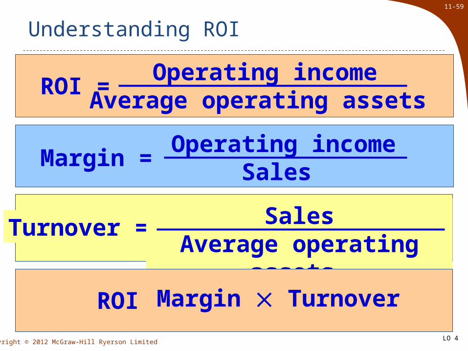
Understanding ROI
ROI = Operating income
Average operating assets
Margin = Operating income
Sales
Turnover = SalesAverage operating
assets ROI = Margin Turnover
LO 4

11-60
Copyright © 2012 McGraw-Hill Ryerson Limited
Increasing ROI
There are three ways to increase ROI . . .There are three ways to increase ROI . . .
IncreaseIncreaseSalesSales
ReduceReduceOperatingOperatingExpensesExpenses ReduceReduce
OperatingOperatingAssetsAssets
LO 4

11-61
Copyright © 2012 McGraw-Hill Ryerson Limited
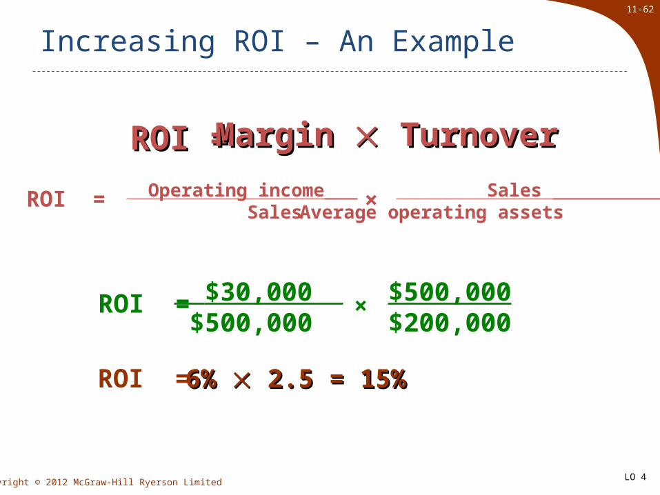
Increasing ROI – An Example
Regal Company reports the following:Regal Company reports the following:
Operating income $ 30,000Operating income $ 30,000
Average operating assets $ 200,000Average operating assets $ 200,000
Sales $ 500,000Sales $ 500,000
Operating expenses $ 470,000Operating expenses $ 470,000
ROI = ROI = Margin Margin Turnover Turnover
Operating income Sales
Sales Average operating assets×ROI =
What is Regal Company’s ROI?
LO 4
11-62
Copyright © 2012 McGraw-Hill Ryerson Limited
Increasing ROI – An Example
$30,000 $500,000
× $500,000$200,000
ROI =
6% 6% 2.5 = 15% 2.5 = 15%ROI =
ROI = ROI = Margin Margin Turnover Turnover
Operating income Sales
Sales Average operating assets×ROI =
LO 4

11-63
Copyright © 2012 McGraw-Hill Ryerson Limited
Increasing Sales Without an Increase in Operating Assets
Regal's manager was able to increase sales to $600,000, while operating expenses increased to $558,000.
Regal's operating income increased to $42,000.
There was no change in the average operating assets of the segment.
Let’s calculate the new ROI.Let’s calculate the new ROI.
LO 4

11-64
Copyright © 2012 McGraw-Hill Ryerson Limited
Increasing Sales Without an Increase in Operating Assets
$42,000 $600,000
× $600,000$200,000
ROI =
7% 7% 3.0 = 21% 3.0 = 21%ROI =
ROI increased from 15% to 21%.ROI increased from 15% to 21%.
ROI = ROI = Margin Margin Turnover Turnover
Operating income Sales
Sales Average operating assets×ROI =
LO 4

11-65
Copyright © 2012 McGraw-Hill Ryerson Limited
Decreasing Operating Expenses with no Change in Sales or Operating Assets
Assume that Regal's manager was able to reduce operating expenses by $10,000, without
affecting sales or operating assets. This would increase operating income to $40,000.
Let’s calculate the new ROI.Let’s calculate the new ROI.
Regal Company reports the following:Regal Company reports the following:
Operating income $ 40,000Operating income $ 40,000
Average operating assets $ 200,000Average operating assets $ 200,000
Sales $ 500,000Sales $ 500,000
Operating expenses $ 460,000Operating expenses $ 460,000
LO 4

11-66
Copyright © 2012 McGraw-Hill Ryerson Limited
Decreasing Operating Expenses with no Change in Sales or Operating Assets
$40,000 $500,000
× $500,000$200,000
ROI =
8% 8% 2.5 = 20% 2.5 = 20%ROI =
ROI increased from 15% to 20%.ROI increased from 15% to 20%.
ROI = ROI = Margin Margin Turnover Turnover
Operating income Sales
Sales Average operating assets×ROI =
LO 4

11-67
Copyright © 2012 McGraw-Hill Ryerson Limited
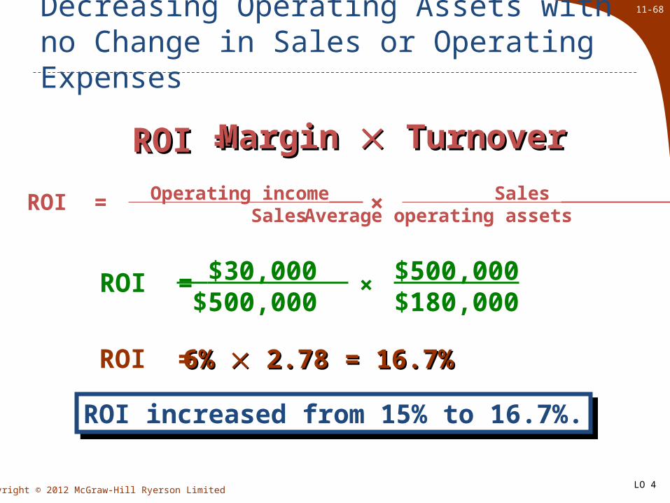
Decreasing Operating Assets with no Change in Sales or Operating Expenses
Assume that Regal's manager was able to reduce inventories by $20,000 using just-in-time
techniques, without affecting sales or operating expenses.
Let’s calculate the new ROI.Let’s calculate the new ROI.
Regal Company reports the following:Regal Company reports the following:
Operating income $ 30,000Operating income $ 30,000
Average operating assets $ 180,000Average operating assets $ 180,000
Sales $ 500,000Sales $ 500,000
Operating expenses $ 470,000Operating expenses $ 470,000
LO 4
11-68
Copyright © 2012 McGraw-Hill Ryerson Limited
Decreasing Operating Assets with no Change in Sales or Operating Expenses
$30,000 $500,000
× $500,000$180,000
ROI =
6% 6% 2.78 = 16.7% 2.78 = 16.7%ROI =
ROI increased from 15% to 16.7%.ROI increased from 15% to 16.7%.
ROI = ROI = Margin Margin Turnover Turnover
Operating income Sales
Sales Average operating assets×ROI =
LO 4
11-69
Copyright © 2012 McGraw-Hill Ryerson Limited
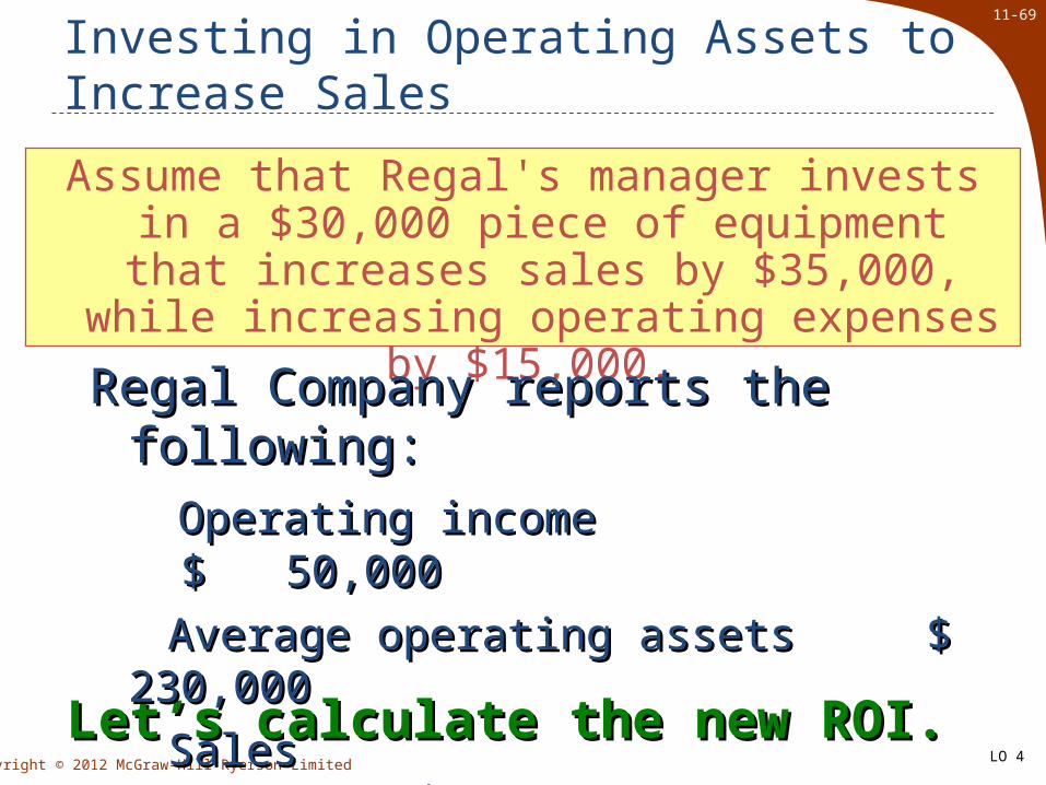
Investing in Operating Assets to Increase Sales
Assume that Regal's manager invests in a $30,000 piece of equipment that increases
sales by $35,000, while increasing operating expenses by $15,000.
Let’s calculate the new ROI.Let’s calculate the new ROI.
Regal Company reports the following:Regal Company reports the following:
Operating income $ 50,000Operating income $ 50,000
Average operating assets $ 230,000Average operating assets $ 230,000
Sales $ 535,000Sales $ 535,000
Operating expenses $ 485,000Operating expenses $ 485,000
LO 4
11-70
Copyright © 2012 McGraw-Hill Ryerson Limited
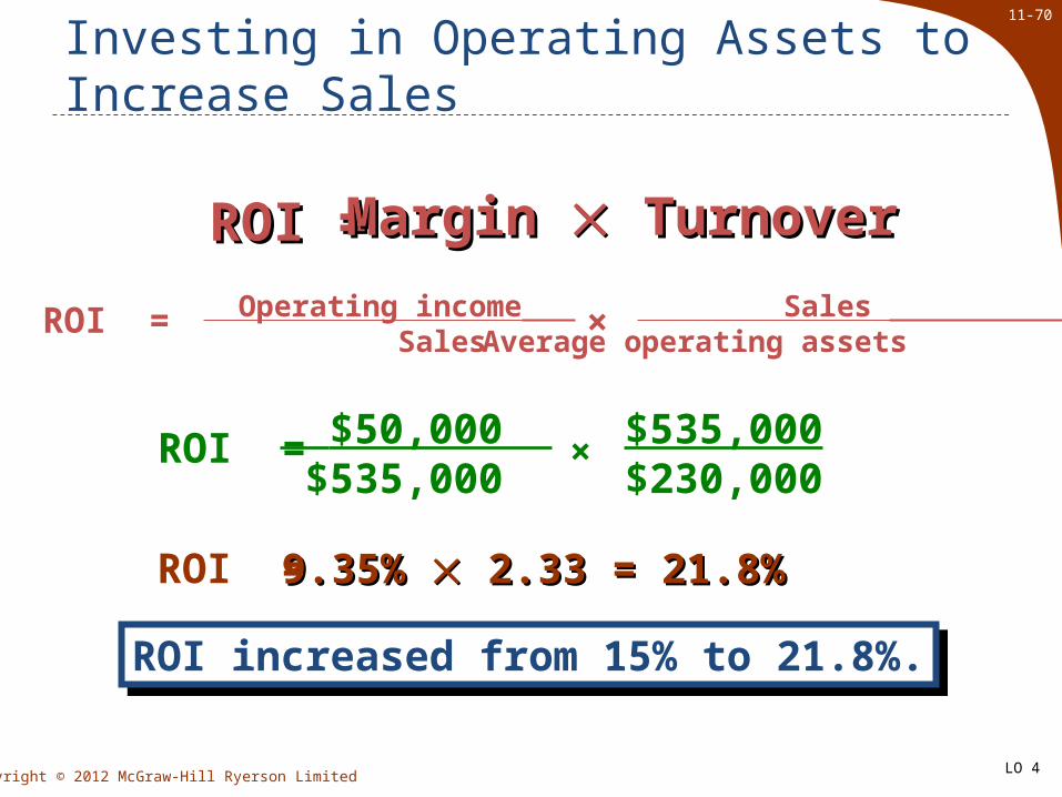
Investing in Operating Assets to Increase Sales
$50,000 $535,000
× $535,000$230,000
ROI =
9.35% 9.35% 2.33 = 21.8% 2.33 = 21.8%ROI =
ROI increased from 15% to 21.8%.ROI increased from 15% to 21.8%.
ROI = ROI = Margin Margin Turnover Turnover
Operating income Sales
Sales Average operating assets×ROI =
LO 4
11-71
Copyright © 2012 McGraw-Hill Ryerson Limited
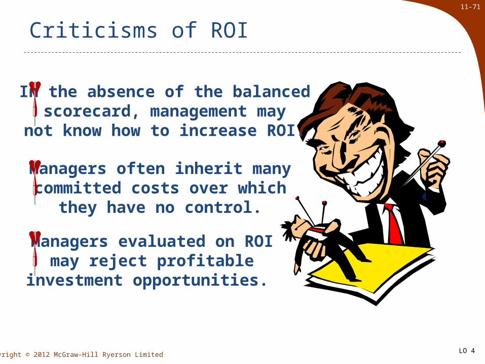
Criticisms of ROI
In the absence of the balancedscorecard, management may
not know how to increase ROI.
Managers often inherit manycommitted costs over which
they have no control.
Managers evaluated on ROImay reject profitable
investment opportunities.
LO 4

11-72
Copyright © 2012 McGraw-Hill Ryerson Limited
Residual Income - Another Measure of Performance
Operating incomeabove some minimum
return on operatingassets
LO 5
11-73
Copyright © 2012 McGraw-Hill Ryerson Limited
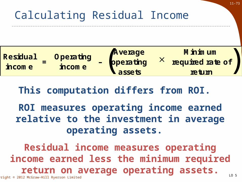
Calculating Residual Income
Residual income
=Operating
income–
Average operating
assets
Minimum
required rate of return( )
This computation differs from ROI.
ROI measures operating income earned relative to the investment in average operating assets.
Residual income measures operating income earned less the minimum required return on
average operating assets.
LO 5

11-74
Copyright © 2012 McGraw-Hill Ryerson Limited
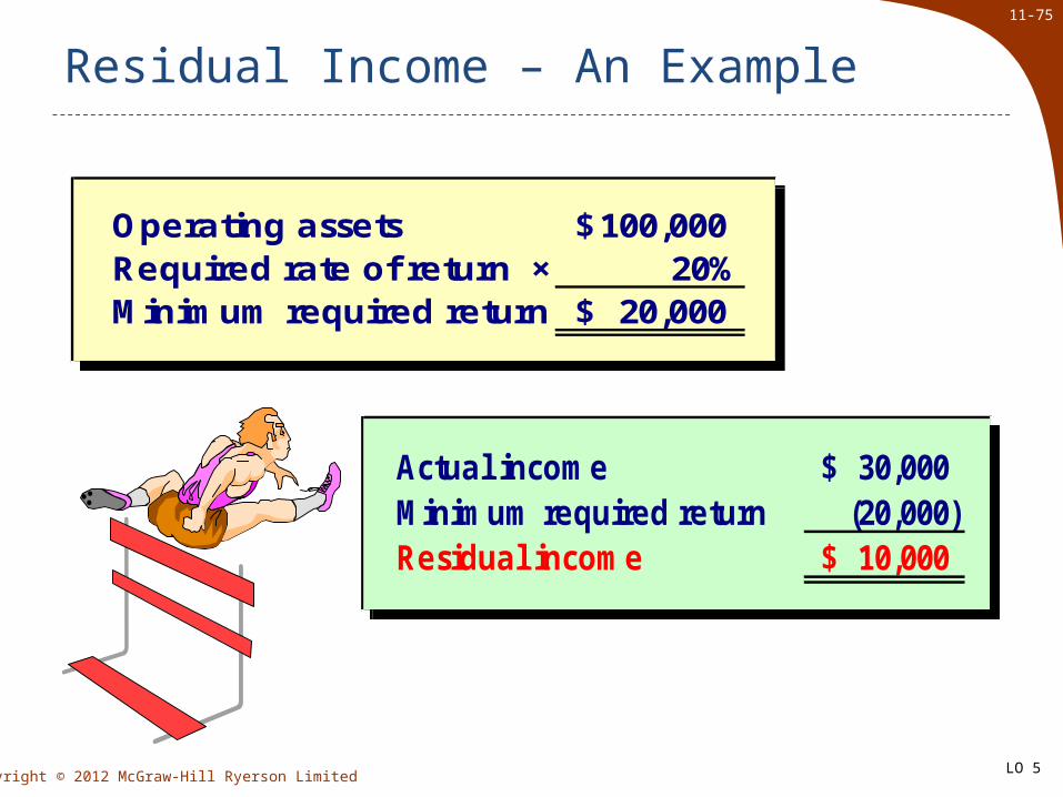
Residual Income – An Example
The Retail Division of Zephyr, Inc. has average operating assets of $100,000 and is required to earn a return of 20% on these assets.
In the current period, the division earns $30,000.
The Retail Division of Zephyr, Inc. has average operating assets of $100,000 and is required to earn a return of 20% on these assets.
In the current period, the division earns $30,000.
Let’s calculate residual income.Let’s calculate residual income.
LO 5
11-75
Copyright © 2012 McGraw-Hill Ryerson Limited
Residual Income – An Example
Operating assets 100,000$ Required rate of return × 20%Minimum required return 20,000$
Operating assets 100,000$ Required rate of return × 20%Minimum required return 20,000$
Actual income 30,000$ Minimum required return (20,000) Residual income 10,000$
Actual income 30,000$ Minimum required return (20,000) Residual income 10,000$
LO 5

11-76
Copyright © 2012 McGraw-Hill Ryerson Limited
Motivation and Residual Income
Residual income encourages managers to make profitable investments that would
be rejected by managers using ROI.
LO 5
11-77
Copyright © 2012 McGraw-Hill Ryerson Limited
Quick Check
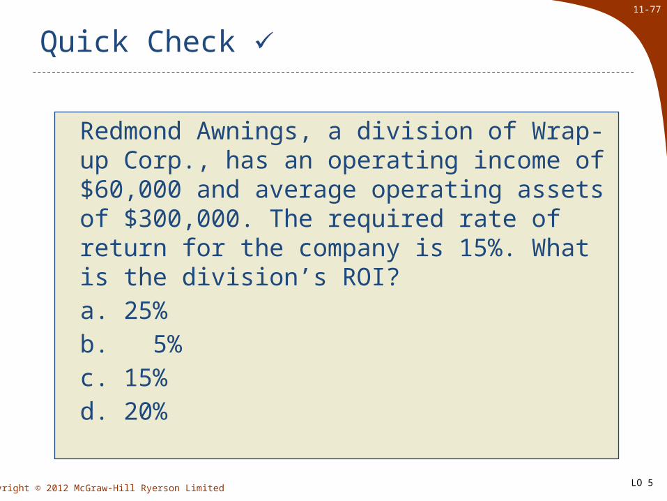
Redmond Awnings, a division of Wrap-up Corp., has an operating income of $60,000 and average operating assets of $300,000. The required rate of return for the company is 15%. What is the division’s ROI?a. 25%b. 5%c. 15%d. 20%
LO 5

11-78
Copyright © 2012 McGraw-Hill Ryerson Limited
Quick Check
Redmond Awnings, a division of Wrap-up Corp., has an operating income of $60,000 and average operating assets of $300,000. The required rate of return for the company is 15%. What is the division’s ROI?a. 25%b. 5%c. 15%d. 20%
ROI = OI / Average operating assets
= $60,000 / $300,000 = 20%
LO 5

11-79
Copyright © 2012 McGraw-Hill Ryerson Limited
Quick Check
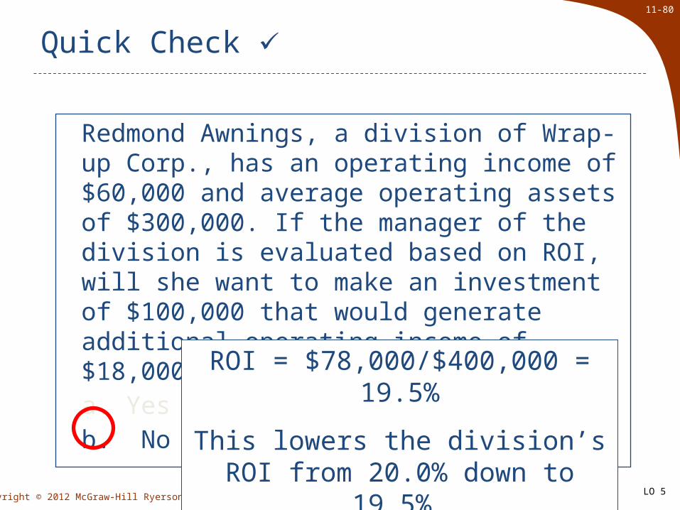
Redmond Awnings, a division of Wrap-up Corp., has an operating income of $60,000 and average operating assets of $300,000. If the manager of the division is evaluated based on ROI, will she want to make an investment of $100,000 that would generate additional operating income of $18,000 per year?a. Yesb. No
LO 5
11-80
Copyright © 2012 McGraw-Hill Ryerson Limited
Quick Check
Redmond Awnings, a division of Wrap-up Corp., has an operating income of $60,000 and average operating assets of $300,000. If the manager of the division is evaluated based on ROI, will she want to make an investment of $100,000 that would generate additional operating income of $18,000 per year?a. Yesb. No
ROI = $78,000/$400,000 = 19.5%
This lowers the division’s ROI from 20.0% down to 19.5%.
LO 5

11-81
Copyright © 2012 McGraw-Hill Ryerson Limited
Quick Check
The company’s required rate of return is 15%. Would the company want the manager of the Redmond Awnings division to make an investment of $100,000 that would generate additional operating income of $18,000 per year?a. Yesb. No
LO 5

11-82
Copyright © 2012 McGraw-Hill Ryerson Limited
Quick Check
The company’s required rate of return is 15%. Would the company want the manager of the Redmond Awnings division to make an investment of $100,000 that would generate additional operating income of $18,000 per year?a. Yesb. No
ROI = $18,000 / $100,000 = 18%
The return on the investment exceeds the minimum required rate
of return.
LO 5

11-83
Copyright © 2012 McGraw-Hill Ryerson Limited
Quick Check
Redmond Awnings, a division of Wrap-up Corp., has an operating income of $60,000 and average operating assets of $300,000. The required rate of return for the company is 15%. What is the division’s residual income?a. $240,000b. $ 45,000c. $ 15,000d. $ 51,000
LO 5

11-84
Copyright © 2012 McGraw-Hill Ryerson Limited
Quick Check
Redmond Awnings, a division of Wrap-up Corp., has an operating income of $60,000 and average operating assets of $300,000. The required rate of return for the company is 15%. What is the division’s residual income?a. $240,000b. $ 45,000c. $ 15,000d. $ 51,000
Operating income $60,000Required return (15% of $300,000) (45,000)Residual income $15,000
LO 5
11-85
Copyright © 2012 McGraw-Hill Ryerson Limited
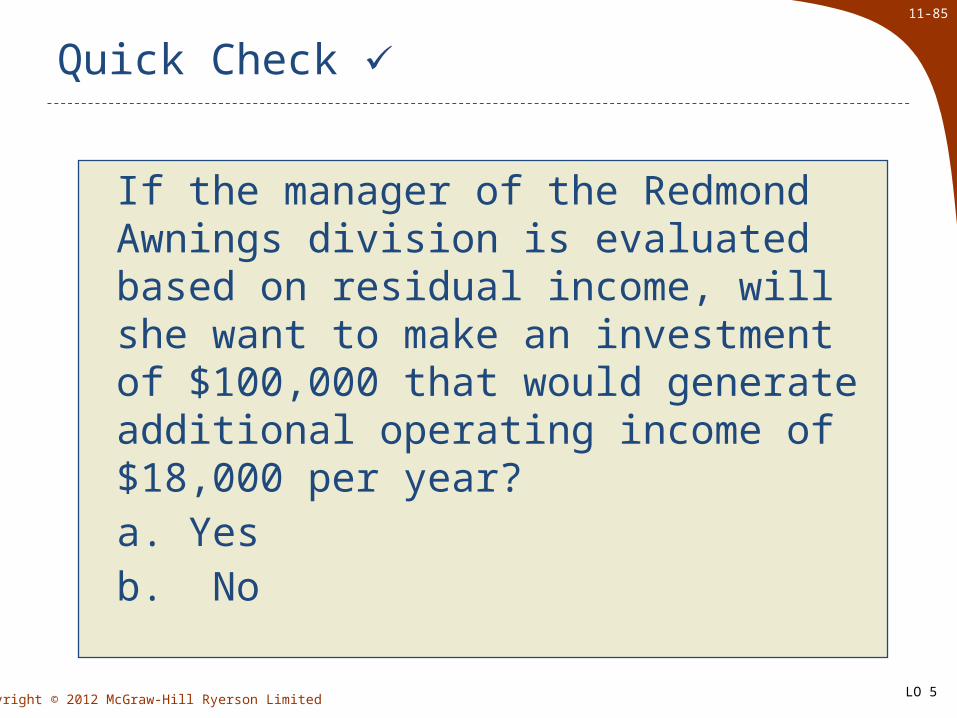
Quick Check
If the manager of the Redmond Awnings division is evaluated based on residual income, will she want to make an investment of $100,000 that would generate additional operating income of $18,000 per year?a. Yesb. No
LO 5

11-86
Copyright © 2012 McGraw-Hill Ryerson Limited
Quick Check
If the manager of the Redmond Awnings division is evaluated based on residual income, will she want to make an investment of $100,000 that would generate additional operating income of $18,000 per year?a. Yesb. No
Operating income $78,000Required return (15% of $400,000) (60,000)Residual income $18,000
Yields an increase of $3,000 in the residual income.
LO 5
11-87
Copyright © 2012 McGraw-Hill Ryerson Limited
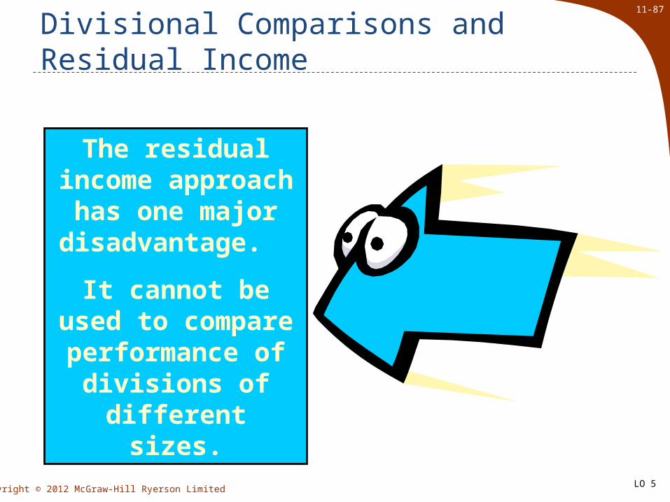
Divisional Comparisons and Residual Income
The residual income approach
has one major disadvantage.
It cannot be used to compare
performance of divisions of
different sizes.
LO 5

11-88
Copyright © 2012 McGraw-Hill Ryerson Limited
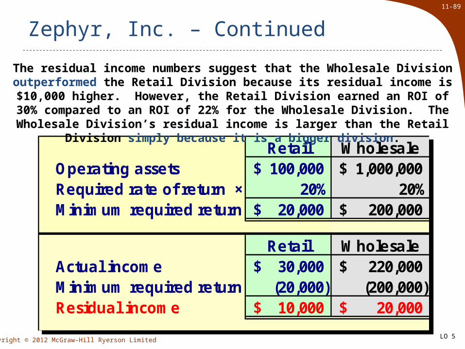
Zephyr, Inc. – Continued
Retail WholesaleOperating assets 100,000$ 1,000,000$ Required rate of return × 20% 20%Minimum required return 20,000$ 200,000$
Retail WholesaleActual income 30,000$ 220,000$ Minimum required return (20,000) (200,000) Residual income 10,000$ 20,000$
Retail WholesaleOperating assets 100,000$ 1,000,000$ Required rate of return × 20% 20%Minimum required return 20,000$ 200,000$
Retail WholesaleActual income 30,000$ 220,000$ Minimum required return (20,000) (200,000) Residual income 10,000$ 20,000$
Recall the following information for the Retail Division of Zephyr, Inc.
Assume the following information for the Wholesale
Division of Zephyr, Inc.
LO 5
11-89
Copyright © 2012 McGraw-Hill Ryerson Limited
Zephyr, Inc. – Continued
Retail WholesaleOperating assets 100,000$ 1,000,000$ Required rate of return × 20% 20%Minimum required return 20,000$ 200,000$
Retail WholesaleActual income 30,000$ 220,000$ Minimum required return (20,000) (200,000) Residual income 10,000$ 20,000$
Retail WholesaleOperating assets 100,000$ 1,000,000$ Required rate of return × 20% 20%Minimum required return 20,000$ 200,000$
Retail WholesaleActual income 30,000$ 220,000$ Minimum required return (20,000) (200,000) Residual income 10,000$ 20,000$
The residual income numbers suggest that the Wholesale Division outperformed the Retail Division because its residual income is $10,000 higher. However, the
Retail Division earned an ROI of 30% compared to an ROI of 22% for the Wholesale Division. The Wholesale Division’s residual income is larger than the
Retail Division simply because it is a bigger division.
LO 5

11-90
Copyright © 2012 McGraw-Hill Ryerson Limited
Criticisms of Residual Income
RI is based on historical accounting data which can lead to inflated amounts for residual income in
periods of rising prices (i.e.. values for capital assets).
RI does not indicate what earnings should be (need comparison of external benchmark or trends).
Calculating RI requires numerous adjustments to GAAP increasing
the cost of preparing information.
RI does not incorporate important leading non-financial indicators.
LO 5

11-91
Copyright © 2012 McGraw-Hill Ryerson Limited
The Balanced Scorecard
Management translates its strategy into performance measures that employees
understand and accept.
Management translates its strategy into performance measures that employees
understand and accept.
Performancemeasures
Customers
Learningand growth
Internalbusiness
processes
Financial
LO 6

11-92
Copyright © 2012 McGraw-Hill Ryerson Limited
The Balanced Scorecard: From Strategy to Performance Measures
Exhibit11-4
FinancialHas our financial
performance improved?
CustomerDo customers recognize that
we are delivering more value?
Internal Business ProcessesHave we improved key business processes so that we can deliver
more value to customers?
Learning and GrowthAre we maintaining our ability
to change and improve?
Performance Measures
What are ourfinancial goals?
What customers dowe want to serve andhow are we going towin and retain them?
What internal busi-ness processes arecritical to providing
value to customers?
Vision and
Strategy
LO 6

11-93
Copyright © 2012 McGraw-Hill Ryerson Limited
The Balanced Scorecard:Non-financial Measures
The balanced scorecard relies on non-financial measures in addition to financial measures for two reasons:
Financial measures are lag indicators that summarize the results of past actions. Non-financial measures are leading indicators of future financial performance.
Financial measures are lag indicators that summarize the results of past actions. Non-financial measures are leading indicators of future financial performance.
Top managers are ordinarily responsible for financial performance measures – not lower level managers. Non-financial measures are more likely to be understood and controlled by lower level managers.
Top managers are ordinarily responsible for financial performance measures – not lower level managers. Non-financial measures are more likely to be understood and controlled by lower level managers.
LO 6
11-94
Copyright © 2012 McGraw-Hill Ryerson Limited
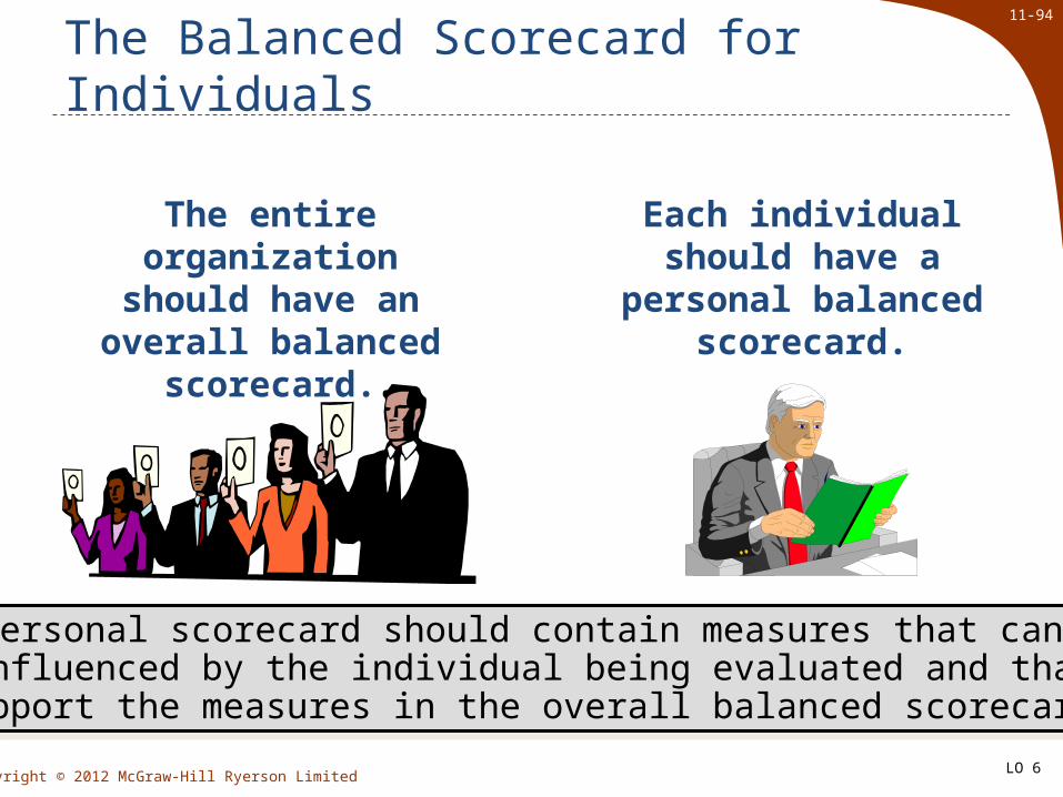
The Balanced Scorecard for Individuals
A personal scorecard should contain measures that can beinfluenced by the individual being evaluated and that
support the measures in the overall balanced scorecard.
A personal scorecard should contain measures that can beinfluenced by the individual being evaluated and that
support the measures in the overall balanced scorecard.
The entire organization should have an overall
balanced scorecard.
Each individual should have a personal
balanced scorecard.
LO 6

11-95
Copyright © 2012 McGraw-Hill Ryerson Limited
The balanced scorecard lays out concrete actions to attain desired outcomes.
A balanced scorecard should have measuresthat are linked together on a cause-and-effect basis.
If we improveone performance
measure . . .
Another desiredperformance measure
will improve.
The Balanced Scorecard
Then
LO 6

11-96
Copyright © 2012 McGraw-Hill Ryerson Limited
The Balanced Scorecardand Compensation
Incentive compensation should be linked to balanced scorecard
performance measures.
LO 6
11-97
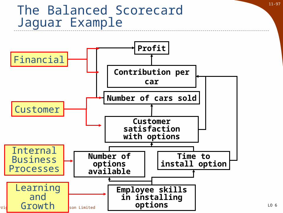
Copyright © 2012 McGraw-Hill Ryerson Limited
The Balanced ScorecardJaguar Example
Employee skills in installing options
Number ofoptions available
Time toinstall option
Customer satisfactionwith options
Number of cars sold
Contribution per car
Profit
Learningand Growth
Internal Business
Processes
Customer
Financial
LO 6

11-98
Copyright © 2012 McGraw-Hill Ryerson Limited
The Balanced ScorecardJaguar Example
Employee skills in installing options
Number ofoptions available
Time toinstall option
Customer satisfactionwith options
Number of cars sold
Contribution per car
Profit
Increase Options Time
Decreases
Strategies
Satisfaction Increases
Increase Skills
Results
LO 6

11-99
Copyright © 2012 McGraw-Hill Ryerson Limited
Employee skills in installing options
Number ofoptions available
Time toinstall option
Customer satisfactionwith options
Number of cars sold
Contribution per car
Profit
Satisfaction Increases
ResultsCars sold Increase
The Balanced ScorecardJaguar Example
LO 6

11-100
Copyright © 2012 McGraw-Hill Ryerson Limited
Employee skills in installing options
Number ofoptions available
Time toinstall option
Customer satisfactionwith options
Number of cars sold
Contribution per car
ProfitResults
The Balanced ScorecardJaguar Example
TimeDecreases
ContributionIncreases
Satisfaction Increases
LO 6

11-101
Copyright © 2012 McGraw-Hill Ryerson Limited
The Balanced ScorecardJaguar Example
Employee skills in installing options
Number ofoptions available
Time toinstall option
Customer satisfactionwith options
Number of cars sold
Contribution per car
ProfitResults
ContributionIncreases
ProfitsIncrease
If numberof cars sold
and contributionper car increase,
profits increase.
Cars Sold Increases
LO 6

11-102
Copyright © 2012 McGraw-Hill Ryerson Limited
Advantages of Graphic Feedback
When interpreting its performance, Jaguar will look forcontinual improvement. It is easier to spot trends or
unusual performance if these data are presented graphically.
Time to Install an Option
0
5
10
15
20
25
30
35
1 2 3 4 5 6 7 8 9 10
Week
Tim
e to
Inst
all i
n M
inu
tes
LO 6

11-103
Copyright © 2012 McGraw-Hill Ryerson Limited
Process time is the only value-added time.
Delivery Performance Measures
Wait TimeProcess Time + Inspection Time
+ Move Time + Queue Time
Delivery Cycle Time
Order Received
ProductionStarted
Goods Shipped
Throughput Time
LO 6

11-104
Copyright © 2012 McGraw-Hill Ryerson Limited
Delivery Performance Measures
ManufacturingCycle
Efficiency
Value-added time
Manufacturing cycle time=
Wait TimeProcess Time + Inspection Time
+ Move Time + Queue Time
Delivery Cycle Time
Order Received
ProductionStarted
Goods Shipped
Throughput Time
LO 6

11-105
Copyright © 2012 McGraw-Hill Ryerson Limited
Quick Check
A TQM team at Narton Corp has recorded the following average times for production:
Wait 3.0 days Move 0.5 days Inspection 0.4 days Queue 9.3 days Process 0.2 days
What is the throughput time?
a. 10.4 daysb. 0.2 daysc. 4.1 daysd. 13.4 days
A TQM team at Narton Corp has recorded the following average times for production:
Wait 3.0 days Move 0.5 days Inspection 0.4 days Queue 9.3 days Process 0.2 days
What is the throughput time?
a. 10.4 daysb. 0.2 daysc. 4.1 daysd. 13.4 days
LO 6

11-106
Copyright © 2012 McGraw-Hill Ryerson Limited
A TQM team at Narton Corp has recorded the following average times for production:
Wait 3.0 days Move 0.5 days Inspection 0.4 days Queue 9.3 days Process 0.2 days
What is the throughput time?
a. 10.4 daysb. 0.2 daysc. 4.1 daysd. 13.4 days
A TQM team at Narton Corp has recorded the following average times for production:
Wait 3.0 days Move 0.5 days Inspection 0.4 days Queue 9.3 days Process 0.2 days
What is the throughput time?
a. 10.4 daysb. 0.2 daysc. 4.1 daysd. 13.4 days
Quick Check
Throughput time = Process + Inspection + Move + Queue = 0.2 days + 0.4 days + 0.5 days + 9.3 days = 10.4 days
LO 6

11-107
Copyright © 2012 McGraw-Hill Ryerson Limited
Quick Check
A TQM team at Narton Corp has recorded the following average times for production:
Wait 3.0 days Move 0.5 days Inspection 0.4 days Queue 9.3 days Process 0.2 days
What is the Manufacturing Cycle Efficiency?
a. 50.0%b. 1.9%c. 52.0%d. 5.1%
A TQM team at Narton Corp has recorded the following average times for production:
Wait 3.0 days Move 0.5 days Inspection 0.4 days Queue 9.3 days Process 0.2 days
What is the Manufacturing Cycle Efficiency?
a. 50.0%b. 1.9%c. 52.0%d. 5.1%
LO 6

11-108
Copyright © 2012 McGraw-Hill Ryerson Limited
A TQM team at Narton Corp has recorded the following average times for production:
Wait 3.0 days Move 0.5 days Inspection 0.4 days Queue 9.3 days Process 0.2 days
What is the Manufacturing Cycle Efficiency?
a. 50.0%b. 1.9%c. 52.0%d. 5.1%
A TQM team at Narton Corp has recorded the following average times for production:
Wait 3.0 days Move 0.5 days Inspection 0.4 days Queue 9.3 days Process 0.2 days
What is the Manufacturing Cycle Efficiency?
a. 50.0%b. 1.9%c. 52.0%d. 5.1%
Quick Check
MCE = Value-added time ÷ Throughput time
= Process time ÷ Throughput time
= 0.2 days ÷ 10.4 days = 1.9%
LO 6

11-109
Copyright © 2012 McGraw-Hill Ryerson Limited
Quick Check
A TQM team at Narton Corp has recorded the following average times for production:
Wait 3.0 days Move 0.5 days Inspection 0.4 days Queue 9.3 days Process 0.2 days
What is the delivery cycle time? a. 0.5 daysb. 0.7 daysc. 13.4 daysd. 10.4 days
A TQM team at Narton Corp has recorded the following average times for production:
Wait 3.0 days Move 0.5 days Inspection 0.4 days Queue 9.3 days Process 0.2 days
What is the delivery cycle time? a. 0.5 daysb. 0.7 daysc. 13.4 daysd. 10.4 days
LO 6

11-110
Copyright © 2012 McGraw-Hill Ryerson Limited
A TQM team at Narton Corp has recorded the following average times for production:
Wait 3.0 days Move 0.5 days Inspection 0.4 days Queue 9.3 days Process 0.2 days
What is the delivery cycle time? a. 0.5 daysb. 0.7 daysc. 13.4 daysd. 10.4 days
A TQM team at Narton Corp has recorded the following average times for production:
Wait 3.0 days Move 0.5 days Inspection 0.4 days Queue 9.3 days Process 0.2 days
What is the delivery cycle time? a. 0.5 daysb. 0.7 daysc. 13.4 daysd. 10.4 days
Quick Check
Delivery cycle time = Wait time + Throughput time = 3.0 days + 10.4 days = 13.4 days
LO 6
11-111
Copyright © 2012 McGraw-Hill Ryerson Limited
ROI and the Balanced Scorecard
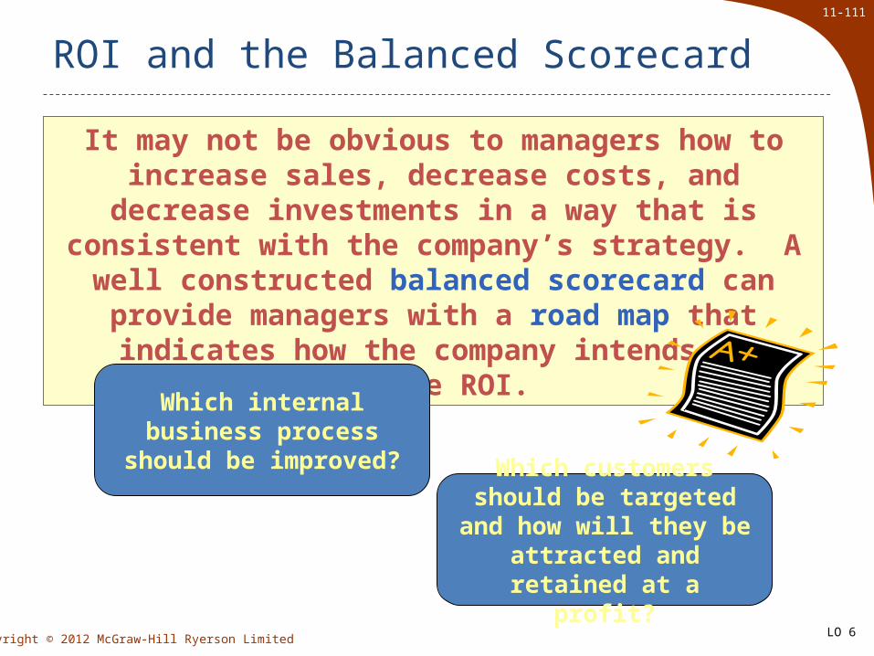
It may not be obvious to managers how to increase sales, decrease costs, and decrease investments in a way that is consistent with the company’s strategy. A
well constructed balanced scorecard can provide managers with a road map that indicates how the
company intends to increase ROI.
Which internal business process should be
improved?
Which customers should be targeted and how will
they be attracted and retained at a profit?
LO 6

11-112
Copyright © 2012 McGraw-Hill Ryerson Limited
Quality of Conformance
When the overwhelming majority of products produced conform to design
specifications and are free from defects.
LO 7

11-113
Copyright © 2012 McGraw-Hill Ryerson Limited
Prevention and Appraisal Costs
Prevention Costs
Support activities whose purpose is to
reduce the number of defects
Appraisal Costs
Incurred to identify defective products
before the products are shipped
LO 7

11-114
Copyright © 2012 McGraw-Hill Ryerson Limited
Internal and External Failure Costs
Internal Failure Costs
Incurred as a result of identifying defects
before they are shipped
External Failure Costs
Incurred as a result of defective products being delivered to
customers
LO 7
11-115
Copyright © 2012 McGraw-Hill Ryerson Limited
Examples of Quality Costs
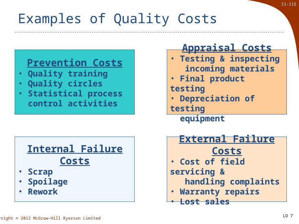
Prevention Costs• Quality training• Quality circles• Statistical process control activities
Appraisal Costs• Testing & inspecting incoming materials• Final product testing• Depreciation of testing equipment
Internal Failure Costs• Scrap• Spoilage• Rework
External Failure Costs• Cost of field servicing & handling complaints• Warranty repairs• Lost sales
LO 7

11-116
Copyright © 2012 McGraw-Hill Ryerson Limited
Distribution of Quality Costs
When quality of conformance is low, total quality cost is high and consists mostly of
internal and external failure.
Total quality costs drop rapidly as the quality of conformance increases.
Companies reduce their total quality costs by focusing their efforts on prevention and appraisal because the cost savings from reduced defects usually overwhelm the
costs of additional prevention and appraisal.
Total quality costs are minimized when the quality of conformance is slightly less
than 100%.LO 7

11-117
Copyright © 2012 McGraw-Hill Ryerson Limited
Quality cost reports provide an estimate of the financial
consequences of the
company’s current defect
rate.
Amount Percent* Amount Percent*Prevention costs:
Systems development 400,000$ 0.80% 270,000$ 0.54%Quality training 210,000 0.42% 130,000 0.26%Supervision of prevention activities 70,000 0.14% 40,000 0.08%Quality improvement 320,000 0.64% 210,000 0.42%
Total prevention cost 1,000,000 2.00% 650,000 1.30%
Appraisal costs:Inspection 600,000 1.20% 560,000 1.12%Reliability testing 580,000 1.16% 420,000 0.84%Supervision of testing and inspection 120,000 0.24% 80,000 0.16%Depreciation of test equipment 200,000 0.40% 140,000 0.28%
Total appraisal cost 1,500,000 3.00% 1,200,000 2.40%
Internal failure costs:Net cost of scrap 900,000 1.80% 750,000 1.50%Rework labor and overhead 1,430,000 2.86% 810,000 1.62%Downtime due to defects in quality 170,000 0.34% 100,000 0.20%Disposal of defective products 500,000 1.00% 340,000 0.68%
Total internal failure cost 3,000,000 6.00% 2,000,000 4.00%
External failure costs:Warranty repairs 400,000 0.80% 900,000 1.80%Warranty replacements 870,000 1.74% 2,300,000 4.60%Allowances 130,000 0.26% 630,000 1.26%Cost of field servicing 600,000 1.20% 1,320,000 2.64%
Total external failure cost 2,000,000 4.00% 5,150,000 10.30%Total quality cost 7,500,000$ 15.00% 9,000,000$ 18.00%
* As a percentage of total sales. In each year sales totaled $50,000,000.
Year 2 Year 1
Quality Cost ReportFor Years 1 and 2
LO 7
11-118
Copyright © 2012 McGraw-Hill Ryerson Limited
Quality Cost Reports in Graphic Form
$10
9
8
7
6
5
4
3
2
1Appraisal
0Prevention Prevention
1 2Year
Qu
alit
y C
ost
(in
mil
lio
ns)
Appraisal
Internal Failure
External Failure
Internal Failure
External Failure
20
18
16
14
12
10
8
6
4
2Appraisal
0Prevention Prevention
1 2Year
Qu
alit
y C
ost
as
a P
erce
nta
ge
of
Sal
es
Appraisal
Internal Failure
External Failure
Internal Failure
External Failure
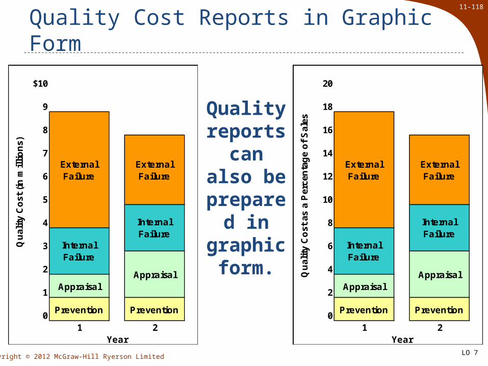
Quality reports
can also be
prepared in
graphic form.
LO 7

11-119
Copyright © 2012 McGraw-Hill Ryerson Limited
Uses of Quality Cost Information
Help managers see the financial significance of
defects.
Help managers identify the relative importance of the quality problems.
Help managers see whether their quality
costs are poorly distributed.
LO 7
11-120
Copyright © 2012 McGraw-Hill Ryerson Limited
Limitations of Quality Cost Information
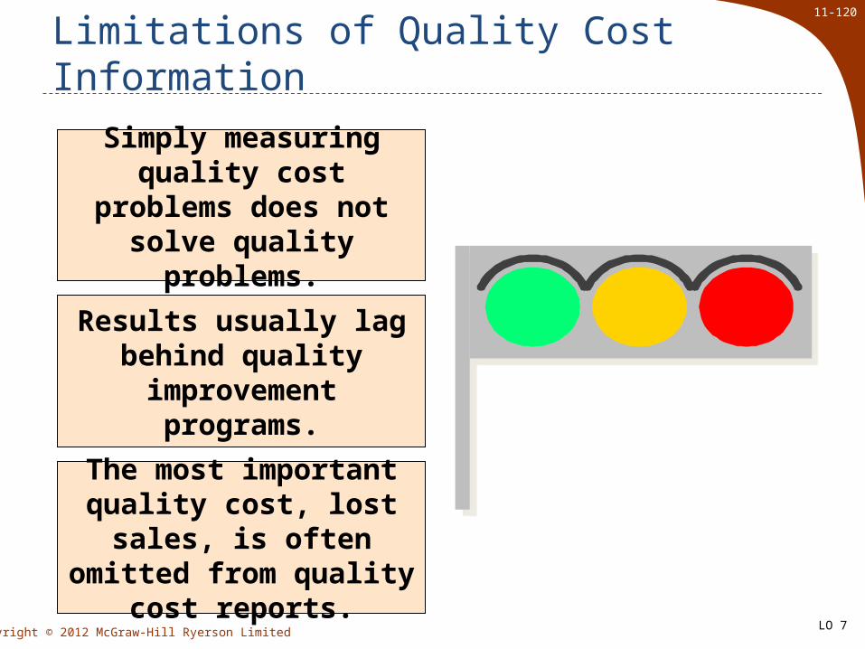
Simply measuring quality cost problems does not solve quality problems.
Results usually lag behind quality
improvement programs.
The most important quality cost, lost sales, is
often omitted from quality cost reports.
LO 7

11-121
Copyright © 2012 McGraw-Hill Ryerson Limited
ISO 9000 Standards
ISO 9000 standards have become international measures of quality.
To become ISO 9000 certified, a company must demonstrate:
1. A quality control system is in use, and the system clearly defines an expected level of quality.
2. The system is fully operational and is backed up with detailed documentation of quality control procedures.
3. The intended level of quality is being achieved on a sustained basis.
LO 7
11-122
Copyright © 2012 McGraw-Hill Ryerson Limited
Profitability Analysis
Appendix 11A
LO 8

11-123
Copyright © 2012 McGraw-Hill Ryerson Limited
Consider the following example for CardCo:Budget Actual
Sales in unitsDeluxe cards 14,000 17,000Standard cards 6,000 5,000
Price per unitDeluxe cards $18 $16Standard cards $ 9 $10
Market volumeDeluxe cards 75,000 85,000Standard cards 95,000 90,000
Variable cost per unitDeluxe cards $ 8 $ 8Standard cards $ 3 $ 3
LO 8
Sales Variance Analysis
11-124
Copyright © 2012 McGraw-Hill Ryerson Limited
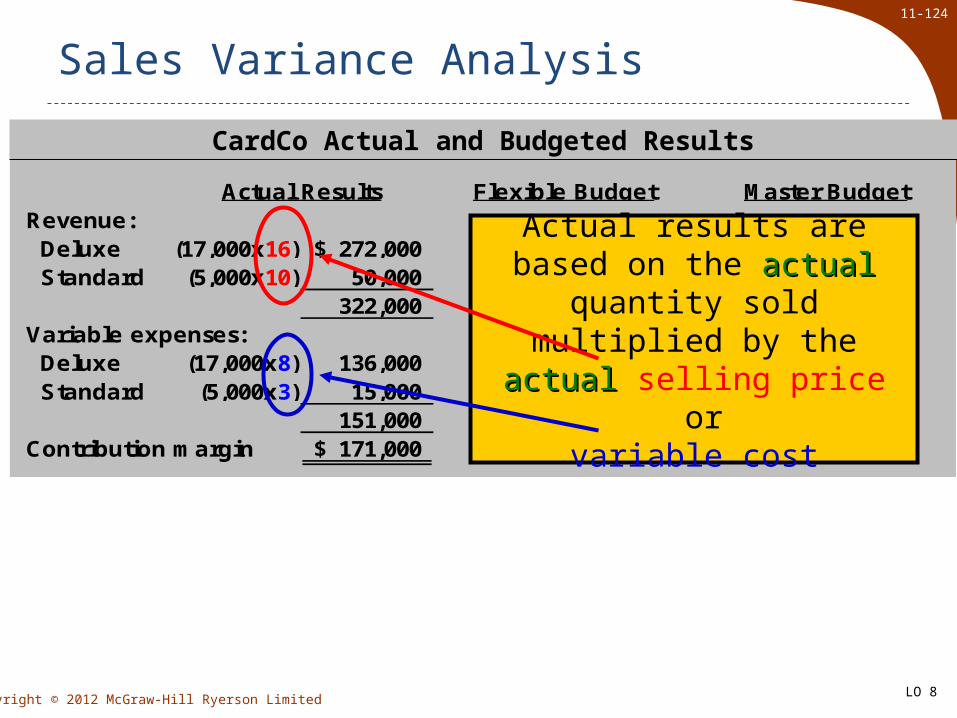
Revenue: Deluxe (17,000x16) 272,000$ Standard (5,000x10) 50,000
322,000 Variable expenses: Deluxe (17,000x8) 136,000 Standard (5,000x3) 15,000
151,000 Contribution margin 171,000$
Actual Results Flexible Budget Master Budget
Actual results are based on the actualactual quantity sold
multiplied by the actual actual selling price or
variable cost
CardCo Actual and Budgeted Results
LO 8
Sales Variance Analysis

11-125
Copyright © 2012 McGraw-Hill Ryerson Limited
Revenue: Deluxe (17,000x16) 272,000$ (17,000x18) 306,000$ Standard (5,000x10) 50,000 (5,000x9) 45,000
322,000 351,000 Variable expenses: Deluxe (17,000x8) 136,000 (17,000x8) 136,000 Standard (5,000x3) 15,000 (5,000x3) 15,000
151,000 151,000 Contribution margin 171,000$ 200,000$
Actual Results Flexible Budget Master Budget
Flexible budget results are based on the actualactual quantity
sold multiplied by the budgetedbudgeted selling price
orvariable cost
CardCo Actual and Budgeted Results
LO 8
Sales Variance Analysis
11-126
Copyright © 2012 McGraw-Hill Ryerson Limited
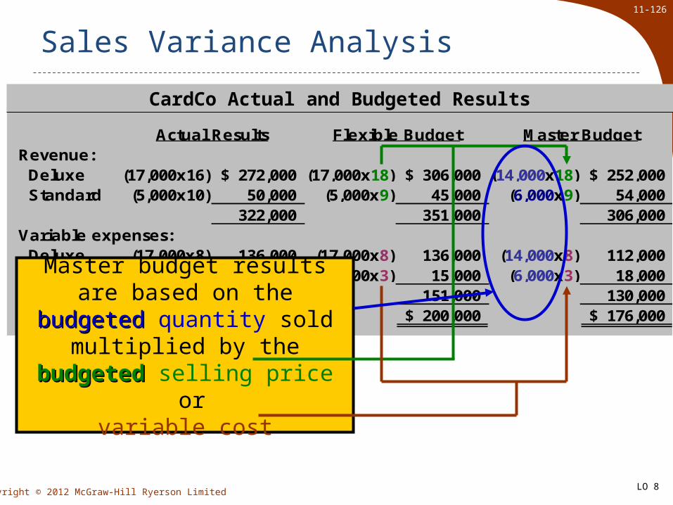
Revenue: Deluxe (17,000x16) 272,000$ (17,000x18) 306,000$ (14,000x18) 252,000$ Standard (5,000x10) 50,000 (5,000x9) 45,000 (6,000x9) 54,000
322,000 351,000 306,000 Variable expenses: Deluxe (17,000x8) 136,000 (17,000x8) 136,000 (14,000x8) 112,000 Standard (5,000x3) 15,000 (5,000x3) 15,000 (6,000x3) 18,000
151,000 151,000 130,000 Contribution margin 171,000$ 200,000$ 176,000$
Actual Results Flexible Budget Master Budget
Master budget results are based on the budgetedbudgeted quantity sold
multiplied by the budgetedbudgeted selling price
orvariable cost
CardCo Actual and Budgeted Results
LO 8
Sales Variance Analysis
11-127
Copyright © 2012 McGraw-Hill Ryerson Limited
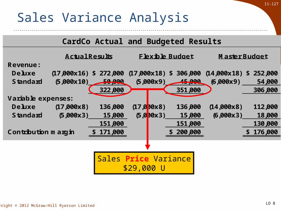
Revenue: Deluxe (17,000x16) 272,000$ (17,000x18) 306,000$ (14,000x18) 252,000$ Standard (5,000x10) 50,000 (5,000x9) 45,000 (6,000x9) 54,000
322,000 351,000 306,000 Variable expenses: Deluxe (17,000x8) 136,000 (17,000x8) 136,000 (14,000x8) 112,000 Standard (5,000x3) 15,000 (5,000x3) 15,000 (6,000x3) 18,000
151,000 151,000 130,000 Contribution margin 171,000$ 200,000$ 176,000$
Actual Results Flexible Budget Master Budget
Sales Price Variance$29,000 U
CardCo Actual and Budgeted Results
LO 8
Sales Variance Analysis

11-128
Copyright © 2012 McGraw-Hill Ryerson Limited
Revenue: Deluxe (17,000x16) 272,000$ (17,000x18) 306,000$ (14,000x18) 252,000$ Standard (5,000x10) 50,000 (5,000x9) 45,000 (6,000x9) 54,000
322,000 351,000 306,000 Variable expenses: Deluxe (17,000x8) 136,000 (17,000x8) 136,000 (14,000x8) 112,000 Standard (5,000x3) 15,000 (5,000x3) 15,000 (6,000x3) 18,000
151,000 151,000 130,000 Contribution margin 171,000$ 200,000$ 176,000$
Actual Results Flexible Budget Master Budget
orSales Price Variance = (Actual – Budgeted price) × Actual sales volume
Deluxe = ($16–$18) × 17,000 units = $34,000 U Standard = ($10–$9) × 5,000 units = $ 5,000 F
Total sales price variance = $29,000 U
$29,000U
CardCo Actual and Budgeted Results
LO 8
Sales Variance Analysis

11-129
Copyright © 2012 McGraw-Hill Ryerson Limited
Revenue: Deluxe (17,000x16) 272,000$ (17,000x18) 306,000$ (14,000x18) 252,000$ Standard (5,000x10) 50,000 (5,000x9) 45,000 (6,000x9) 54,000
322,000 351,000 306,000 Variable expenses: Deluxe (17,000x8) 136,000 (17,000x8) 136,000 (14,000x8) 112,000 Standard (5,000x3) 15,000 (5,000x3) 15,000 (6,000x3) 18,000
151,000 151,000 130,000 Contribution margin 171,000$ 200,000$ 176,000$
Actual Results Flexible Budget Master Budget
Sales Volume Variance$24,000 F
CardCo Actual and Budgeted Results
LO 8
Sales Variance Analysis

11-130
Copyright © 2012 McGraw-Hill Ryerson Limited
Revenue: Deluxe (17,000x16) 272,000$ (17,000x18) 306,000$ (14,000x18) 252,000$ Standard (5,000x10) 50,000 (5,000x9) 45,000 (6,000x9) 54,000
322,000 351,000 306,000 Variable expenses: Deluxe (17,000x8) 136,000 (17,000x8) 136,000 (14,000x8) 112,000 Standard (5,000x3) 15,000 (5,000x3) 15,000 (6,000x3) 18,000
151,000 151,000 130,000 Contribution margin 171,000$ 200,000$ 176,000$
Actual Results Flexible Budget Master Budget
CardCo Actual and Budgeted Results
orSales Volume Variance= (Actual – Budgeted quantity) × Budgeted CM
Deluxe = (17,000–14,000) × ($18–$8) units = $30,000 F Standard = (5,000–6,000) × ($9–$3) = $ 6,000 U
Total sales volume variance = $24,000 F
$24,000F
LO 8
Sales Variance Analysis

11-131
Copyright © 2012 McGraw-Hill Ryerson Limited
The Sales VolumeVolume Variance can further be broken down into the: Market VolumeVolume Variance
=
Market ShareShare Variance
=
Budgeted CM per
unit
Actual market volume
Budget market volume
–{ } ×
Budgeted CM per
unit×
Actual market share
–Expected
market share }{
×Expected
market share %
Actual sales
quantity–[ ]
LO 8
Sales Variance Analysis

11-132
Copyright © 2012 McGraw-Hill Ryerson Limited
For CardCo, the Sales VolumeVolume Variance of $24,000 F breakdown further as follows: Market VolumeVolume VarianceDeluxe = (85,000–75,000) × (14,000/75,000) × (18–8) = 18,667 F
Standard = (90,000–95,000) × (6,000/95,000) × (9–3) = 1,895 U
Total Market Volume Variance (1) 16,772 F16,772 F Market ShareShare VarianceDeluxe = [17,000–(85,000 × 14,000/75,000)] × (18–8) = 11,333 F
Standard = [5,000–(90,000 × 6,000/95,000)] × (9–3) = 4,105 U
Total Market Share Variance (2) 7,228 F7,228 F
Sales VolumeVolume Variance = (1) + (2) = 24,000 F
LO 8
Sales Variance Analysis

11-133
Copyright © 2012 McGraw-Hill Ryerson Limited
The Sales VolumeVolume Variance can also be broken down into the: Sales MixMix Variance
=
Sales QuantityQuantity Variance
=
Actual sales quantity
Actual sales quantity at
expected sales mix
Budgeted CM per unit
–{ }×
Actual sales quantity at
expected sales mix
– Anticipated sales quantity} Budgeted CM
per unit×{
LO 8
Sales Variance Analysis

11-134
Copyright © 2012 McGraw-Hill Ryerson Limited
For CardCo, the Sales VolumeVolume Variance of $24,000F is made up of: Sales MixMix VarianceDeluxe = [17,000–(22,000 × 14/20)] × (18–8)=16,000 F
Standard = [5,000–(22,000 × 6/20)] × (9–3) = 9,600 U
Total Sales Mix Variance (1) 6,400 F6,400 F Sales QuantityQuantity VarianceDeluxe = [(22,000 × 14/20)–14,000] × (18–8)=14,000 F
Standard = [(22,000 × 6/20)–6,000] × (9–3) = 3,600 F
Total Sales Quantity Variance (2) 17,600F17,600F
Sales VolumeVolume Variance = (1) + (2) = 24,000F
LO 8
Sales Variance Analysis

11-135
Copyright © 2012 McGraw-Hill Ryerson Limited
Marketing Expense
Appendix 11B
LO 9

11-136
Copyright © 2012 McGraw-Hill Ryerson Limited
Marketing Strategy
Transport Warehousing
SellingAdvertising
Credit
LO 9
Costs Factors to Consider in a Marketing Strategy
11-137
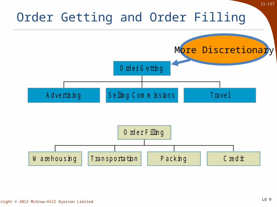
Copyright © 2012 McGraw-Hill Ryerson Limited
Order Getting and Order Filling
A d vertis in g S e llin g C om m iss ion s Trave l
O rd er G e tt in g
W areh ou s in g Tran sp orta tion P ack in g C red it
O rd er F illin g
More Discretionary
LO 9

11-138
Copyright © 2012 McGraw-Hill Ryerson Limited
End of Chapter 11