copyright © 2009 pearson education, inc. 6- 1 topic 3. chapters 6 & 7 supply of labor
Post on 20-Dec-2015
220 views
TRANSCRIPT

Copyright © 2009 Pearson Education, Inc. 6- 1
Topic 3. Chapters 6 & 7
Supply of Labor

Copyright © 2009 Pearson Education, Inc. 6- 2
Labor Force Participation Rates (LFPR)
Population (P) = Employment (E) + Unemployment (U) + Out of labor force (O)
LFPR = {(E+U) / P}*100Unemployment Rate (UR) = {U/(E+U)}*100

Copyright © 2009 Pearson Education, Inc. 6- 3
Table 6.1: Labor Force Participation Rates of Females in the United States over 16 Years of
Age, by Martial Status, 1900-2005 (percentage)

Copyright © 2009 Pearson Education, Inc. 6- 4
Table 6.2: Labor Force Participation Rates for Male in the United States, by Age,
1900-2005 (percentage)
Copyright © 2009 Pearson Education, Inc. 6- 5
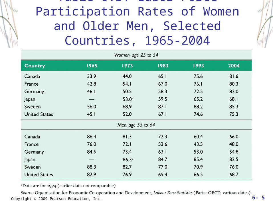
Table 6.3: Labor Force Participation Rates of Women and Older Men, Selected Countries, 1965-2004 (percentage)
Copyright © 2009 Pearson Education, Inc. 6- 6
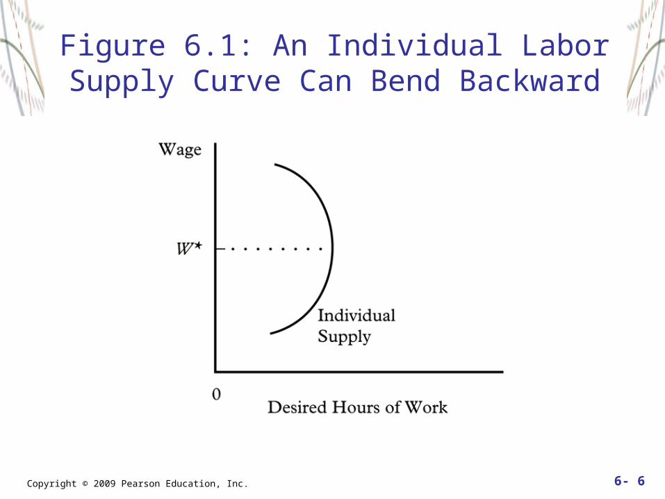
Figure 6.1: An Individual Labor Supply Curve Can Bend Backward

Copyright © 2009 Pearson Education, Inc. 6- 7
Figure 6.2: Two Indifference Curves for the Same Person
Copyright © 2009 Pearson Education, Inc. 6- 8
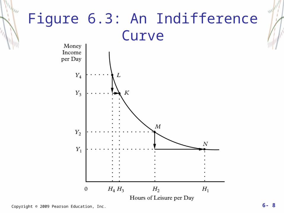
Figure 6.3: An Indifference Curve

Copyright © 2009 Pearson Education, Inc. 6- 9
Figure 6.4: Indifference Curves for Two Different People

Copyright © 2009 Pearson Education, Inc. 6- 10
Figure 6.5: Indifference Curve and Budget Constraint

Copyright © 2009 Pearson Education, Inc. 6- 11
Exercise 1: How to Draw a Budget Constraint (and an optimal choice of labor supply)?
1. You can supply up to 16 hours of labor a day. Your current hourly wage rate is $8 per hour (and no other income). Draw your budget line.
2. Draw an indifference curve showing that your optimal daily labor supply at this wage is 9 hours.

Copyright © 2009 Pearson Education, Inc. 6- 12
Figure 6.6: The Decision Not to Work is a “Corner Solution”

Copyright © 2009 Pearson Education, Inc. 6- 13
Exercise 2. How to Draw a Budget Constraint with an increase in non-labor income
1. You can supply up to 16 hours of labor a day. Your current hourly wage rate is $8 per hour (and no other income). Your rich aunt gives you $36 every day as an allowance;
2. Draw a budget constraint and an indifference curve showing that your optimal daily labor supply at this wage decreased from 9 hours to 8 hours.

Copyright © 2009 Pearson Education, Inc. 6- 14
Figure 6.7: Indifference Curves and Budget Constraint (with an increase in nonlabor
income)

Copyright © 2009 Pearson Education, Inc. 6- 15
Exercise 3: How to Draw a Budget Constraint with an increase in wage?
1. You can supply up to 16 hours of labor a day. Your current hourly wage rate is $8 per hour (and no other income) and you work 8 hours per day. Your wage increases to $12 per hour. Amend the budget constraint
2. Draw an indifference curve showing that your optimal daily labor supply at the new wage increases from 8 hours to 11 hours.

Copyright © 2009 Pearson Education, Inc. 6- 16
Figure 6.8: Wage Increase with Substitution Effect Dominating

Copyright © 2009 Pearson Education, Inc. 6- 17
Figure 6.9: Wage Increase with Income Effect Dominating

Copyright © 2009 Pearson Education, Inc. 6- 18
Figure 6.10a: Wage Increase with Substitution Effect Dominating: Isolating
Income and Substitution Effects

Copyright © 2009 Pearson Education, Inc. 6- 19
Figure 6.10b: Wage Increase with Substitution Effect Dominating: Isolating
Income and Substitution Effects

Copyright © 2009 Pearson Education, Inc. 6- 20
Figure 6.10c: Wage Increase with Substitution Effect Dominating: Isolating
Income and Substitution Effects

Copyright © 2009 Pearson Education, Inc. 6- 21
Figure 6.12: Reservation Wage with Fixed Time Costs of Working
Copyright © 2009 Pearson Education, Inc. 6- 22
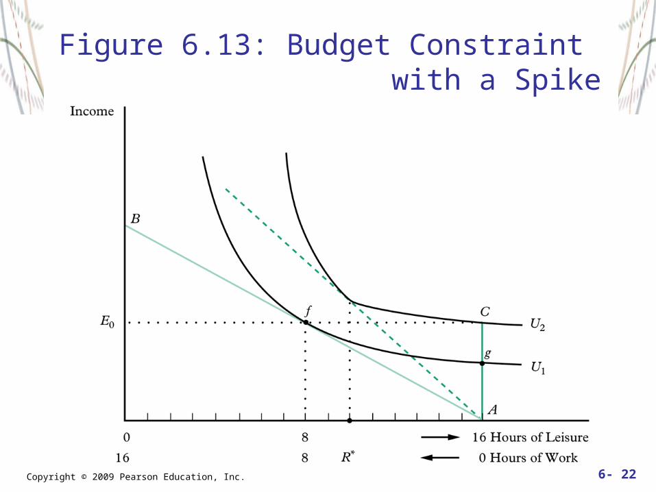
Figure 6.13: Budget Constraint with a Spike

Copyright © 2009 Pearson Education, Inc. 6- 23
Figure 6.14: Income and Substitution Effects for the Basic Welfare System

Copyright © 2009 Pearson Education, Inc. 6- 24
Figure 6.15: The Basic Welfare System: A Person Not Choosing Welfare

Copyright © 2009 Pearson Education, Inc. 6- 25
Figure 6.16: The Welfare System with a Work Requirement
Copyright © 2009 Pearson Education, Inc. 6- 26
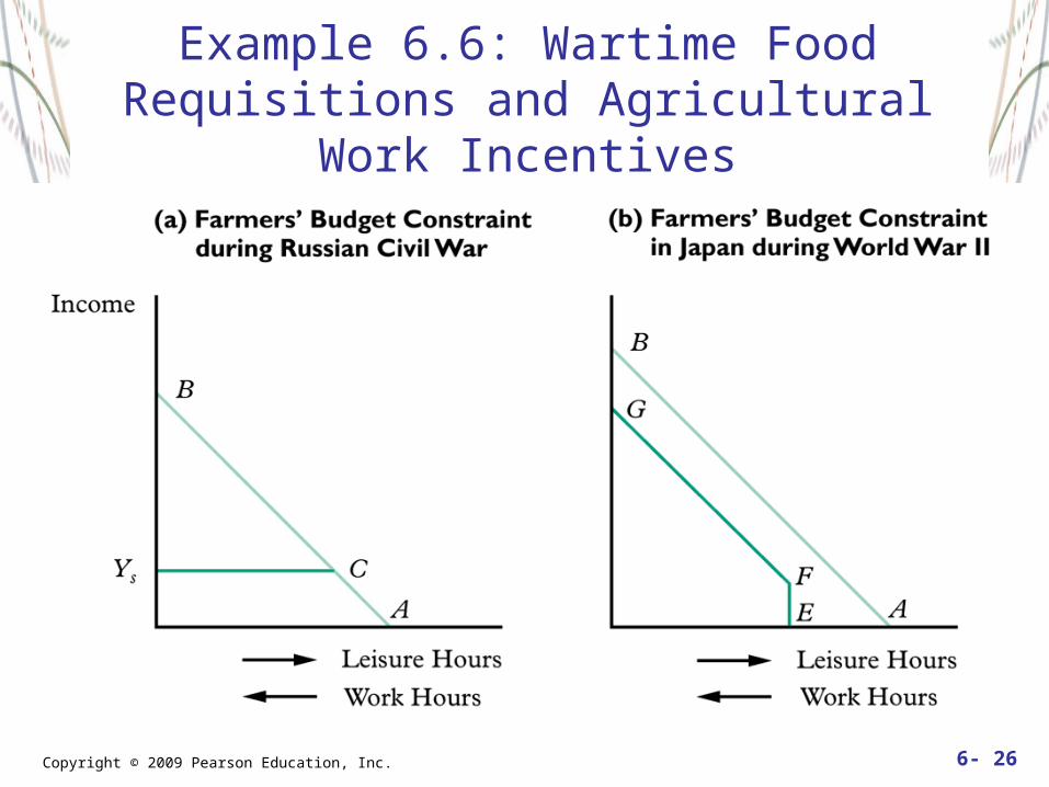
Example 6.6: Wartime Food Requisitions and Agricultural Work Incentives
Copyright © 2009 Pearson Education, Inc. 6- 27
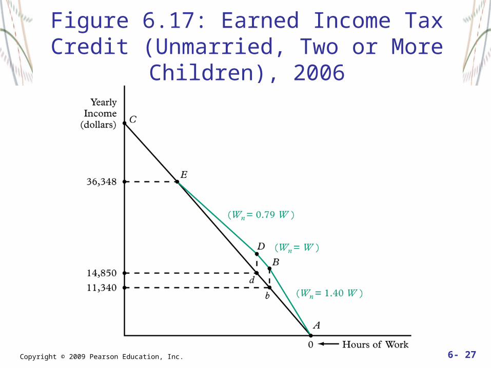
Figure 6.17: Earned Income Tax Credit (Unmarried, Two or More Children), 2006
Copyright © 2009 Pearson Education, Inc. 6- 28
Other Examples
Overtime payMoonlighting
Copyright © 2009 Pearson Education, Inc. 6- 29
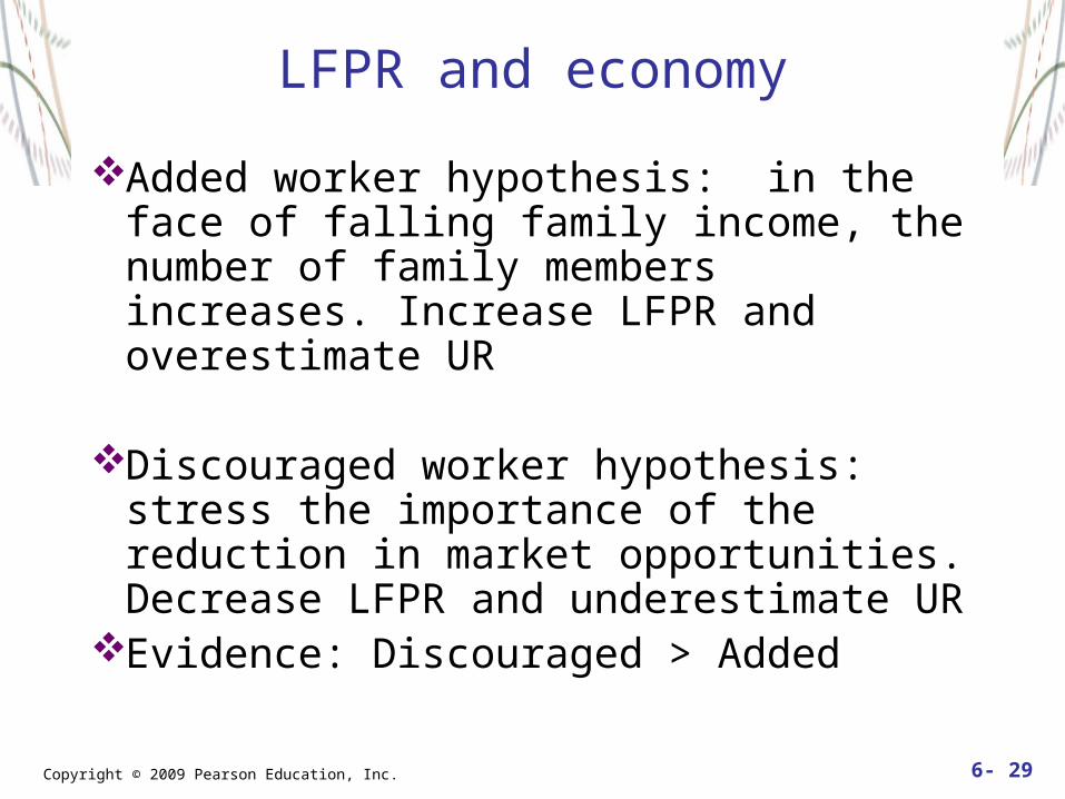
LFPR and economy
Added worker hypothesis: in the face of falling family income, the number of family members increases. Increase LFPR and overestimate UR
Discouraged worker hypothesis: stress the importance of the reduction in market opportunities. Decrease LFPR and underestimate UR
Evidence: Discouraged > Added

Copyright © 2009 Pearson Education, Inc. 6- 30
LFP Revisited
w* (reservation wage=slope of indifference curve)
w (market wage=slope of budget constraint) then work
w* > w then do not work, and vice versaExplain the trend of female LFPR (Table
6.2) using w* and w (education, affirmative action, fertility, divorce rate, technological change, etc)

Copyright © 2009 Pearson Education, Inc. 6- 31
Factors affecting the distribution of works in a household
Wage rateNumber of young kidsSubstitution of mother’s time (baby sitting, A
plus program, washing machines, etc.)Sudden increase in non-labor incomeThe future value of kids/spouse

Copyright © 2009 Pearson Education, Inc. 6- 32
Table 7.1: Weekly Hours Spent in Household Work, Paid Work, and Leisure Activities by
Men and Women over Age 18, 2005
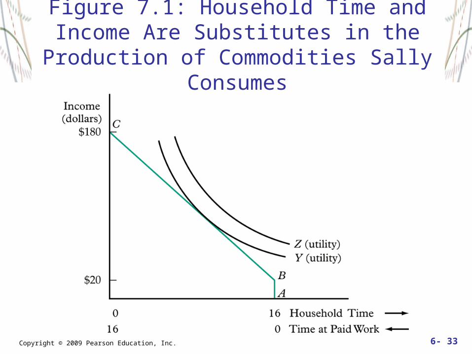
Copyright © 2009 Pearson Education, Inc. 6- 33
Figure 7.1: Household Time and Income Are Substitutes in the Production of
Commodities Sally Consumes

Copyright © 2009 Pearson Education, Inc. 6- 34
Table 7.2: Labor Force Participation Rates and Full-Time Employment, Mothers of Young Children, by Age of Child, 2006
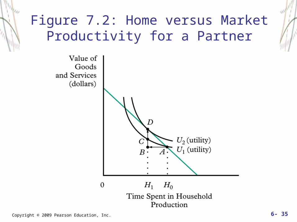
Copyright © 2009 Pearson Education, Inc. 6- 35
Figure 7.2: Home versus Market Productivity for a Partner

Copyright © 2009 Pearson Education, Inc. 6- 36
Figure 7.3: Life-Cycle Allocation of Time

Copyright © 2009 Pearson Education, Inc. 6- 37
Table 7.3: Assumed Social Security Benefits and Earnings for a Hypothetical Male, Age 62
(yearly wage = $40,000; Interest rate = 2%; life expectancy = 17 years)

Copyright © 2009 Pearson Education, Inc. 6- 38
Figure 7.4:
Choice of Optimum
Retirement Age for
Hypothetical Worker
(based on data in Table 7.3)

Copyright © 2009 Pearson Education, Inc. 6- 39
Figure 7.5: Labor Supply and Fixed Child-Care Costs: A Parent Initially
Out of the Labor Force
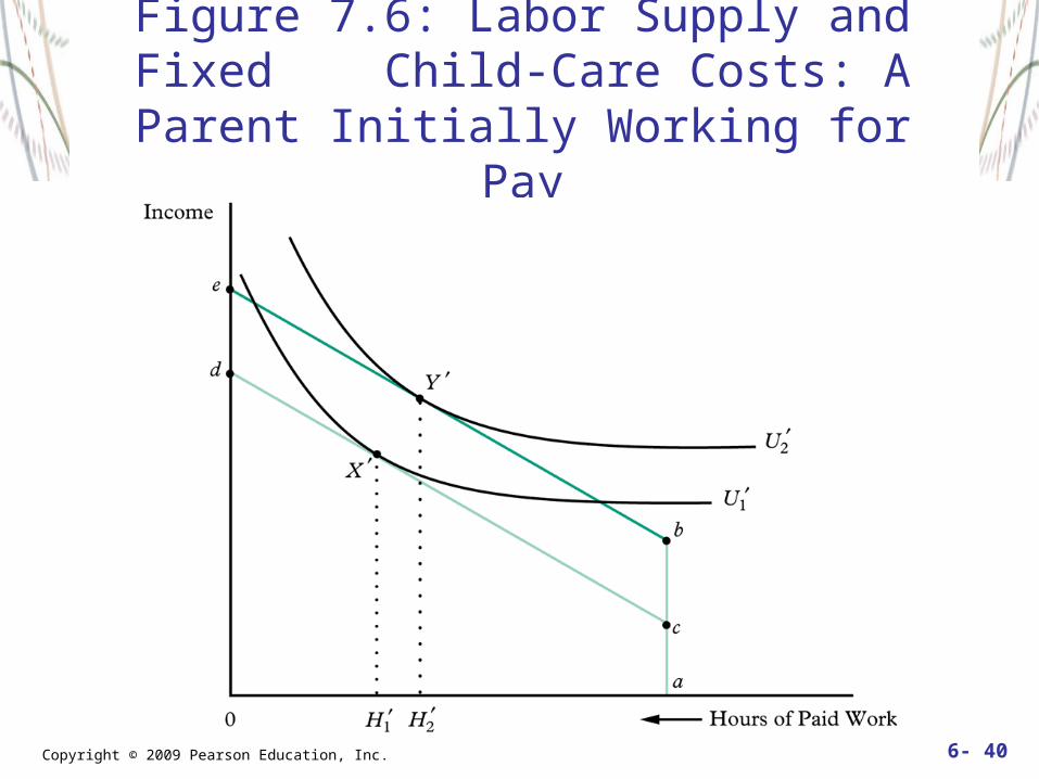
Copyright © 2009 Pearson Education, Inc. 6- 40
Figure 7.6: Labor Supply and Fixed Child-Care Costs: A Parent Initially
Working for Pay

Copyright © 2009 Pearson Education, Inc. 6- 41
Figure 7.7: Budget Constraints Facing a Single Parent before and after Child
Support Assurance Program Adopted

Copyright © 2009 Pearson Education, Inc. 6- 42
Figure 7.8: A Single Parent Who Joins the Labor Force after Child Support
Assurance Program Adopted