copyright ©2005 brooks/cole a division of thomson learning, inc. introduction to probability and...

Copyright ©2005 Brooks/ColeA division of Thomson Learning, Inc.

Introduction to Probability Introduction to Probability and Statisticsand Statistics

Twelfth EditionTwelfth Edition

Robert J. Beaver • Barbara M. Beaver • William Mendenhall

Presentation designed and written by: Presentation designed and written by: Barbara M. BeaverBarbara M. Beaver


Introduction to Probability Introduction to Probability and Statisticsand Statistics

Twelfth EditionTwelfth Edition

Chapter 3

Describing Bivariate Data

Some images © 2001-(current year) www.arttoday.com


Bivariate DataBivariate Data• When two variables are measured on a single

experimental unit, the resulting data are called bivariate data.bivariate data.

• You can describe each variable individually, and you can also explore the relationshiprelationship between the two variables.

• Bivariate data can be described with

– GraphsGraphs

– Numerical MeasuresNumerical Measures


Graphs for Qualitative Graphs for Qualitative VariablesVariables

• When at least one of the variables is qualitative, you can use comparative pie charts comparative pie charts or bar charts.or bar charts.

Variable #1 =

Variable #2 =

Do you think that men and women are treated equally in the workplace?

Do you think that men and women are treated equally in the workplace?

Opinion

Gender

WomenMen


Comparative Bar ChartsComparative Bar Charts

• Stacked Bar ChartStacked Bar Chart

Percent

OpinionGender

No OpinionDisagreeAgreeWomenMenWomenMenWomenMen

70

60

50

40

30

20

10

0

Percent

OpinionGender

No OpinionDisagreeAgreeWomenMenWomenMenWomenMen

70

60

50

40

30

20

10

0

• Side-by-Side Bar ChartSide-by-Side Bar ChartDescribe the relationship between opinion and gender:

More women than men feel that they are not treated equally in the workplace..

More women than men feel that they are not treated equally in the workplace..

Percent

Opinion No OpinionDisagreeAgree

120

100

80

60

40

20

0

GenderMenWomen

Percent

Opinion No OpinionDisagreeAgree

120

100

80

60

40

20

0

GenderMenWomen


Two Quantitative VariablesTwo Quantitative VariablesWhen both of the variables are quantitative, call one variable x and the other y. A single measurement is a pair of numbers (x, y) that can be plotted using a two-dimensional graph called a scatterplot.scatterplot.

y

x

(2, 5)

x = 2

y = 5


• What pattern pattern or form form do you see?

• Straight line upward or downward

• Curve or no pattern at all

• How strongstrong is the pattern?

• Strong or weak

• Are there any unusual observationsunusual observations?

• Clusters or outliers

Describing the ScatterplotDescribing the Scatterplot


Positive linear - strong Negative linear -weak

Curvilinear No relationship

ExamplesExamples


Numerical Measures for Numerical Measures for Two Quantitative VariablesTwo Quantitative Variables

• Assume that the two variables x and y exhibit a linear pattern linear pattern or formform.

• There are two numerical measures to describe

– The strength strength and direction direction of the relationship between x and y.

– The form form of the relationship.


The Correlation CoefficientThe Correlation Coefficient• The strength and direction of the relationship

between x and y are measured using the correlation coefficient, correlation coefficient, rr..

where

sx = standard deviation of the x’s

sy = standard deviation of the y’s

sx = standard deviation of the x’s

sy = standard deviation of the y’s

yx

xy

ss

sr

yx

xy

ss

sr

1

))((

nn

yxyx

s

iiii

xy 1

))((

nn

yxyx

s

iiii

xy


• Living area x and selling price y of 5 homes.

ExampleExample

Residence 1 2 3 4 5

x (hundred sq ft) 14 15 17 19 16

y ($000) 178 230 240 275 200

•The scatterplot indicates a positive linear relationship.

•The scatterplot indicates a positive linear relationship.


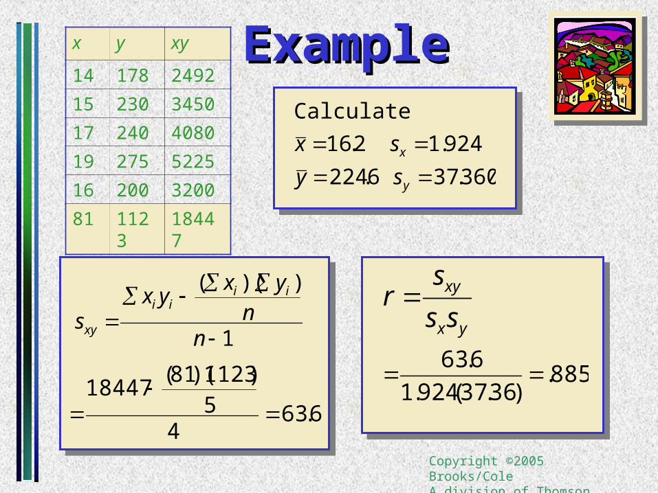
ExampleExamplex y xy

14 178 2492

15 230 3450

17 240 4080

19 275 5225

16 200 3200

81 1123 18447

360.37 6.224

924.1 2.16

Calculate

y

x

sy

sx

1

))((

nn

yxyx

s

iiii

xy

6.634

5)1123)(81(

18447

yx

xy

ss

sr

885.)36.37(924.1

6.63


Interpreting Interpreting rr

All points fall exactly on a straight line.

Strong relationship; either positive or negative

Weak relationship; random scatter of points

•-1 r 1

•r 0

•r 1 or –1

•r = 1 or –1

Sign of r indicates direction of the linear relationship.

APPLETAPPLETMY


The Regression LineThe Regression Line• Sometimes x and y are related in a particular way

—the value of y dependsdepends on the value of x.– y = dependent variable– x = independent variable

• The form of the linear relationship between x and y can be described by fitting a line as best we can through the points. This is the regression line, regression line,

yy = = aa + + bxbx..– a = y-intercept of the line– b = slope of the line

APPLETAPPLETMY


The Regression LineThe Regression Line• To find the slope and y-intercept of

the best fitting line, use:

xbya

s

srb

x

y

xbya

s

srb

x

y

• The least squares

• regression line is y = a + bx


x

y

s

srb

xby a

ExampleExamplex y xy

14 178 2492

15 230 3450

17 240 4080

19 275 5225

16 200 3200

81 1123 18447885.

3604.376.224

9235.12.16

r

sy

sx

y

x

Recall

189.179235.1

3604.37)885(.

86.53)2.16(189.176.224

xy 189.1786.53 :Line Regression


Predict:

ExampleExample

xy 189.1786.53

• Predict the selling price for another residence with 1600 square feet of living area.

)16(189.1786.53 $221,160or 16.221


Key ConceptsKey ConceptsI. Bivariate DataI. Bivariate Data

1. Both qualitative and quantitative variables

2. Describing each variable separately3. Describing the relationship between the variables

II. Describing Two Qualitative VariablesII. Describing Two Qualitative Variables1. Side-by-Side pie charts2. Comparative line charts3. Comparative bar chartsSide-by-SideStacked

4. Relative frequencies to describe the relationship between the two variables.


Key ConceptsKey ConceptsIII. Describing Two Quantitative VariablesIII. Describing Two Quantitative Variables

1. Scatterplots

Linear or nonlinear pattern

Strength of relationship

Unusual observations; clusters and outliers

2. Covariance and correlation coefficient

3. The best fitting line

Calculating the slope and y-intercept

Graphing the line

Using the line for prediction

copyright ©2005 brooks/cole a division of thomson learning, inc. introduction to probability and...

Documents