copyright © 2004 by limsoon wong gene finding & gene feature recognition by computational...
TRANSCRIPT

Cop
yrig
ht ©
200
4 by
Lim
soon
Won
g
Gene Finding & Gene Feature
Recognition by Computational
Analysis
Limsoon WongInstitute for Infocomm
ResearchNovember 2004

Copyright © 2004 by Limsoon Wong
Lecture Plan
• Gene structure basics• Gene finding overview• GRAIL• Indel & frame-shift in coding regions• Histone promoters: A cautionary case
study• Knowledge discovery basics• TIS recognition• Poly-A signal recognition• TSS recognition
Basic materials
Advanced materials

Cop
yrig
ht ©
200
4 by
Lim
soon
Won
g
Gene Structure Basics
A brief refresher
Some slides here are “borrowed” from Ken Sung

Copyright © 2004 by Limsoon Wong
Body
• Our body consists of a number of organs• Each organ composes of a number of
tissues• Each tissue composes of cells of the
same type

Copyright © 2004 by Limsoon Wong
Cell
• Performs two types of function– Chemical reactions necessary to maintain our
life– Pass info for maintaining life to next
generation
• In particular– Protein performs chemical reactions– DNA stores & passes info– RNA is intermediate between DNA & proteins
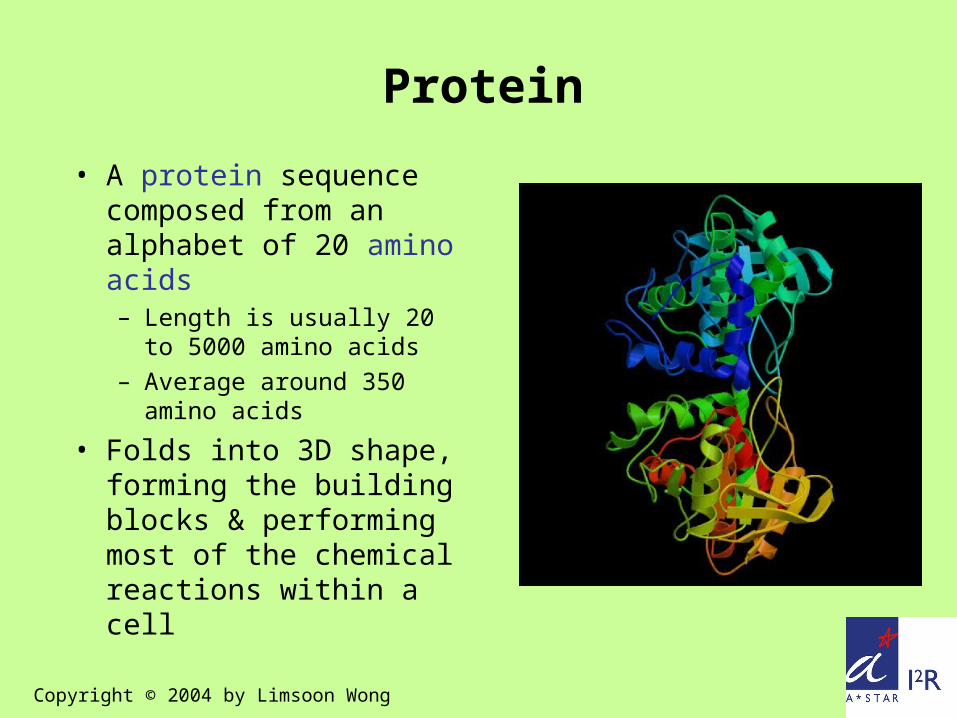
Protein
• A protein sequence composed from an alphabet of 20 amino acids– Length is usually 20 to
5000 amino acids – Average around 350
amino acids
• Folds into 3D shape, forming the building blocks & performing most of the chemical reactions within a cell
Copyright © 2004 by Limsoon Wong

Amino Acid
• Each amino acid consist of– Amino group– Carboxyl group– R group
Carboxyl group
Aminogroup
C
(the central carbon)R group
NH2
H
C C
R
OH
O
Copyright © 2004 by Limsoon Wong

Copyright © 2004 by Limsoon Wong
Classification of Amino Acids
• Amino acids can be classified into 4 types.
• Positively charged (basic)– Arginine (Arg, R)– Histidine (His, H)– Lysine (Lys, K)
• Negatively charged (acidic)– Aspartic acid (Asp, D)– Glutamic acid (Glu, E)

Copyright © 2004 by Limsoon Wong
Classification of Amino Acids• Polar (overall
uncharged, but uneven charge distribution. can form hydrogen bonds with water. they are called hydrophilic)– Asparagine (Asn, N)– Cysteine (Cys, C)– Glutamine (Gln, Q)– Glycine (Gly, G)– Serine (Ser, S)– Threonine (Thr, T)– Tyrosine (Tyr, Y)
• Nonpolar (overall uncharged and uniform charge distribution. cant form hydrogen bonds with water. they are called hydrophobic)– Alanine (Ala, A)– Isoleucine (Ile, I)– Leucine (Leu, L)– Methionine (Met, M)– Phenylalanine (Phe, F)– Proline (Pro, P)– Tryptophan (Trp, W)– Valine (Val, V)

N
H
C C
R’
OH
O
NH2
H
C C
R
O
H
Peptide bond
NH2
H
C C
R
OH
O
NH2
H
C C
R’
OH
O
+
Protein & Polypeptide Chain
• Formed by joining amino acids via peptide bond• One end the amino group, called N-terminus• The other end is the carboxyl group, called C-
terminus
Copyright © 2004 by Limsoon Wong
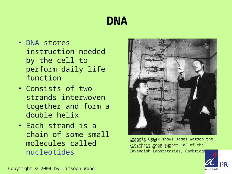
DNA
• DNA stores instruction needed by the cell to perform daily life function
• Consists of two strands interwoven together and form a double helix
• Each strand is a chain of some small molecules called nucleotides
Francis Crick shows James Watson the model of DNA in their room number 103 of the Austin Wing at the Cavendish Laboratories, Cambridge
Copyright © 2004 by Limsoon Wong
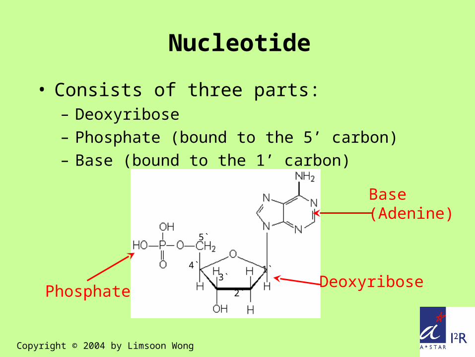
Base(Adenine)
DeoxyribosePhosphate
5`
4`3`
2`
1`
Nucleotide
• Consists of three parts:– Deoxyribose– Phosphate (bound to the 5’ carbon)– Base (bound to the 1’ carbon)
Copyright © 2004 by Limsoon Wong
A C G T U
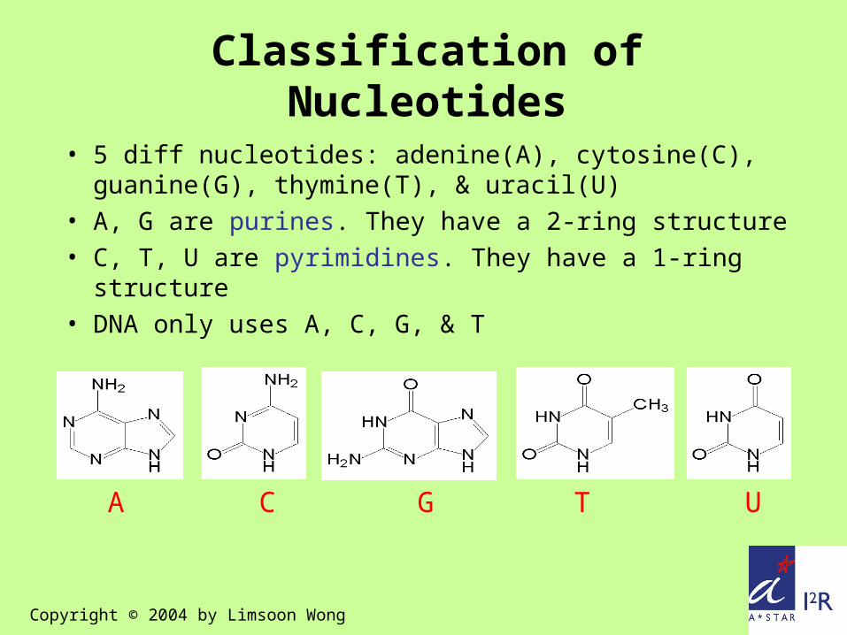
Classification of Nucleotides
• 5 diff nucleotides: adenine(A), cytosine(C), guanine(G), thymine(T), & uracil(U)
• A, G are purines. They have a 2-ring structure• C, T, U are pyrimidines. They have a 1-ring
structure• DNA only uses A, C, G, & T
Copyright © 2004 by Limsoon Wong

A
T
10Å
G
C
10Å
Watson-Crick rules
• Complementary bases:– A with T (two hydrogen-bonds)– C with G (three hydrogen-bonds)
Copyright © 2004 by Limsoon Wong

P P P P
5’3’
A C G T A
Orientation of a DNA
• One strand of DNA is generated by chaining together nucleotides, forming a phosphate-sugar backbone
• It has direction: from 5’ to 3’, because DNA always extends from 3’ end:– Upstream, from 5’ to 3’– Downstream, from 3’ to 5’
Copyright © 2004 by Limsoon Wong

Double Stranded DNA
• DNA is double stranded in a cell. The two strands are anti-parallel. One strand is reverse complement of the other
• The double strands are interwoven to form a double helix
Copyright © 2004 by Limsoon Wong

Copyright © 2004 by Limsoon Wong
Locations of DNAs in a Cell?
• Two types of organisms– Prokaryotes (single-celled organisms with no nuclei. e.g.,
bacteria)
– Eukaryotes (organisms with single or multiple cells. their cells have nuclei. e.g., plant & animal)
• In Prokaryotes, DNA swims within the cell• In Eukaryotes, DNA locates within the
nucleus

Copyright © 2004 by Limsoon Wong
Chromosome
• DNA is usually tightly wound around histone proteins and forms a chromosome
• The total info stored in all chromosomes constitutes a genome
• In most multi-cell organisms, every cell contains the same complete set of chromosomes – May have some small different due to
mutation
• Human genome has 3G base pairs, organized in 23 pairs of chromosomes

Copyright © 2004 by Limsoon Wong
Gene
• A gene is a sequence of DNA that encodes a protein or an RNA molecule
• About 30,000 – 35,000 (protein-coding) genes in human genome
• For gene that encodes protein– In Prokaryotic genome, one gene corresponds
to one protein– In Eukaryotic genome, one gene can
corresponds to more than one protein because of the process “alternative splicing”

Copyright © 2004 by Limsoon Wong
Complexity of Organism vs. Genome Size
• Human Genome: 3G base pairs
• Amoeba dubia (a single cell organism): 600G base pairs
Genome size has no relationship with the complexity of the organism
Copyright © 2004 by Limsoon Wong
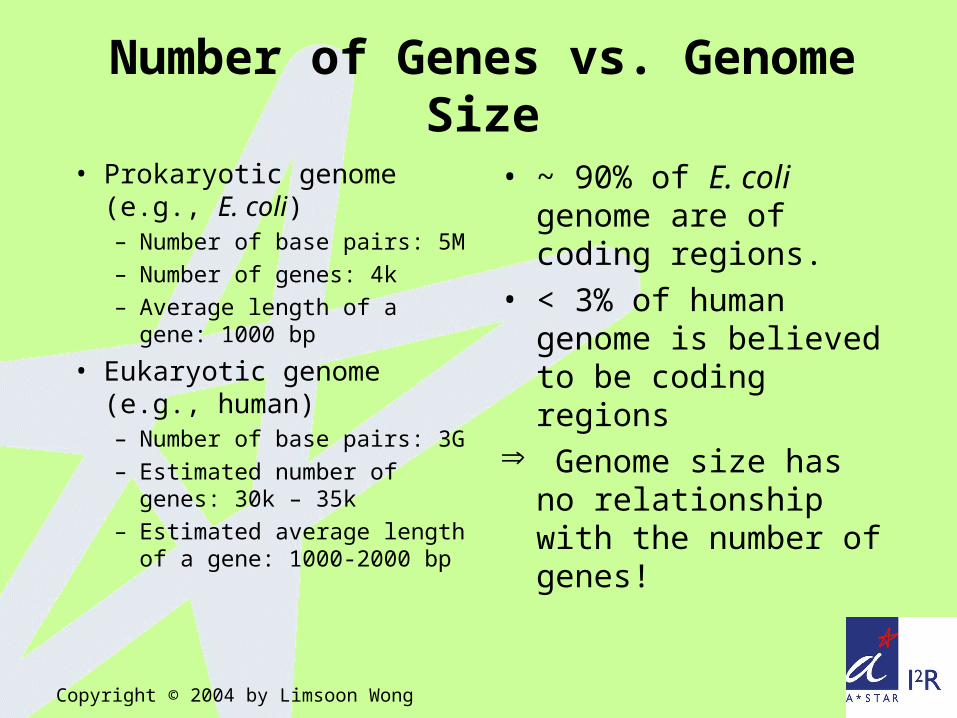
Number of Genes vs. Genome Size
• Prokaryotic genome (e.g., E. coli)– Number of base pairs: 5M– Number of genes: 4k– Average length of a gene:
1000 bp
• Eukaryotic genome (e.g., human)– Number of base pairs: 3G– Estimated number of
genes: 30k – 35k– Estimated average length
of a gene: 1000-2000 bp
• ~ 90% of E. coli genome are of coding regions.
• < 3% of human genome is believed to be coding regions
Genome size has no relationship with the number of genes!

Base(Adenine)
Ribose SugarPhosphate
5`
4`3`
2`
1`
RNA
• RNA has both the properties of DNA & protein– Similar to DNA, it can
store & transfer info– Similar to protein, it
can form complex 3D structure & perform some functions
• Nucleotide for RNA has of three parts:– Ribose Sugar (has an
extra OH group at 2’)– Phosphate (bound to 5’
carbon)– Base (bound to 1’
carbon)
Copyright © 2004 by Limsoon Wong
Copyright © 2004 by Limsoon Wong
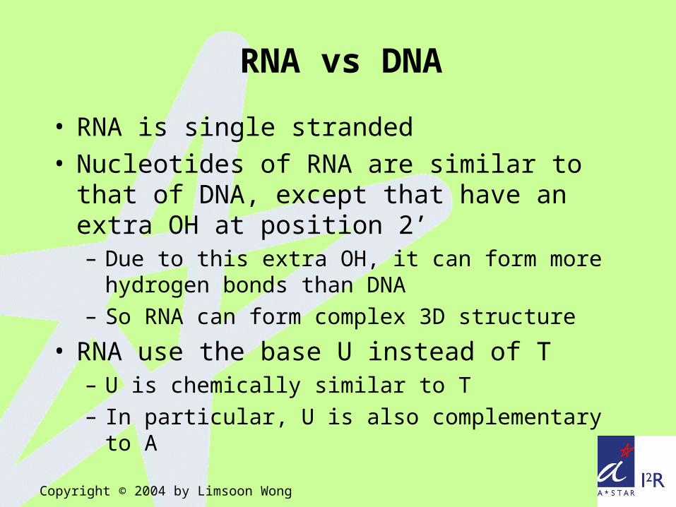
RNA vs DNA
• RNA is single stranded• Nucleotides of RNA are similar to that of
DNA, except that have an extra OH at position 2’– Due to this extra OH, it can form more
hydrogen bonds than DNA– So RNA can form complex 3D structure
• RNA use the base U instead of T– U is chemically similar to T– In particular, U is also complementary to A

Mutation
• Mutation is a sudden change of genome
• Basis of evolution• Cause of cancer• Can occur in DNA,
RNA, & Protein
Copyright © 2004 by Limsoon Wong

Central Dogma
• Gene expression consists of two steps– Transcription
DNA mRNA
– Translation mRNA Protein
Copyright © 2004 by Limsoon Wong

Copyright © 2004 by Limsoon Wong
Transcription
• Synthesize mRNA from one strand of DNA– An enzyme RNA
polymerase temporarily separates double-stranded DNA
– It begins transcription at transcription start site
– A A, CC, GG, & TU
– Once RNA polymerase reaches transcription stop site, transcription stops
• Additional “steps” for Eukaryotes– Transcription produces
pre-mRNA that contains both introns & exons
– 5’ cap & poly-A tail are added to pre-mRNA
– RNA splicing removes introns & mRNA is made
– mRNA are transported out of nucleus

Copyright © 2004 by Limsoon Wong
Translation
• Synthesize protein from mRNA
• Each amino acid is encoded by consecutive seq of 3 nucleotides, called a codon
• The decoding table from codon to amino acid is called genetic code
• 43=64 diff codons Codons are not 1-to-1
corr to 20 amino acids• All organisms use the
same decoding table• Recall that amino acids
can be classified into 4 groups. A single-base change in a codon is usually not sufficient to cause a codon to code for an amino acid in different group

Genetic Code• Start codon: ATG (code for M)• Stop codon: TAA, TAG, TGA
Copyright © 2004 by Limsoon Wong

Copyright © 2004 by Limsoon Wong
Ribosome
• Translation is handled by a molecular complex, ribosome, which consists of both proteins & ribosomal RNA (rRNA)
• Ribosome reads mRNA & the translation starts at a start codon (the translation start site)
• With help of tRNA, each codon is translated to an amino acid
• Translation stops once ribosome reads a stop codon (the translation stop site)
Copyright © 2004 by Limsoon Wong
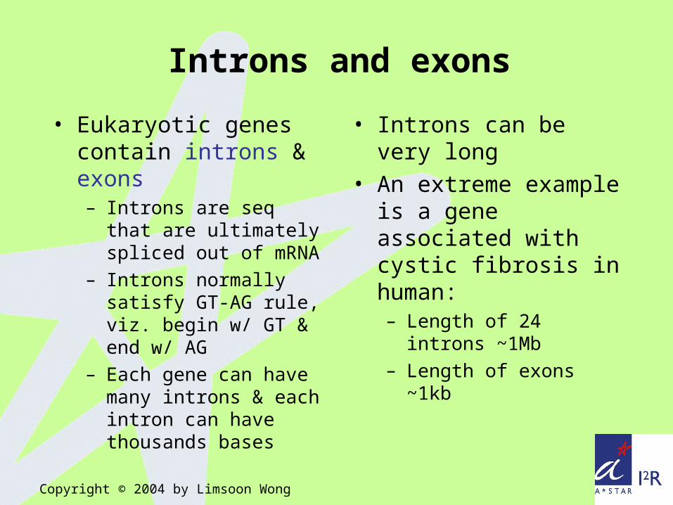
Introns and exons
• Eukaryotic genes contain introns & exons– Introns are seq that
are ultimately spliced out of mRNA
– Introns normally satisfy GT-AG rule, viz. begin w/ GT & end w/ AG
– Each gene can have many introns & each intron can have thousands bases
• Introns can be very long
• An extreme example is a gene associated with cystic fibrosis in human:– Length of 24 introns
~1Mb– Length of exons ~1kb

• Unlike eukaryotic genes, a prokaryotic gene typically consists of only one contiguous coding region
Typical Eukaryotic Gene Structure
Copyright © 2004 by Limsoon Wong
Image credit: Xu
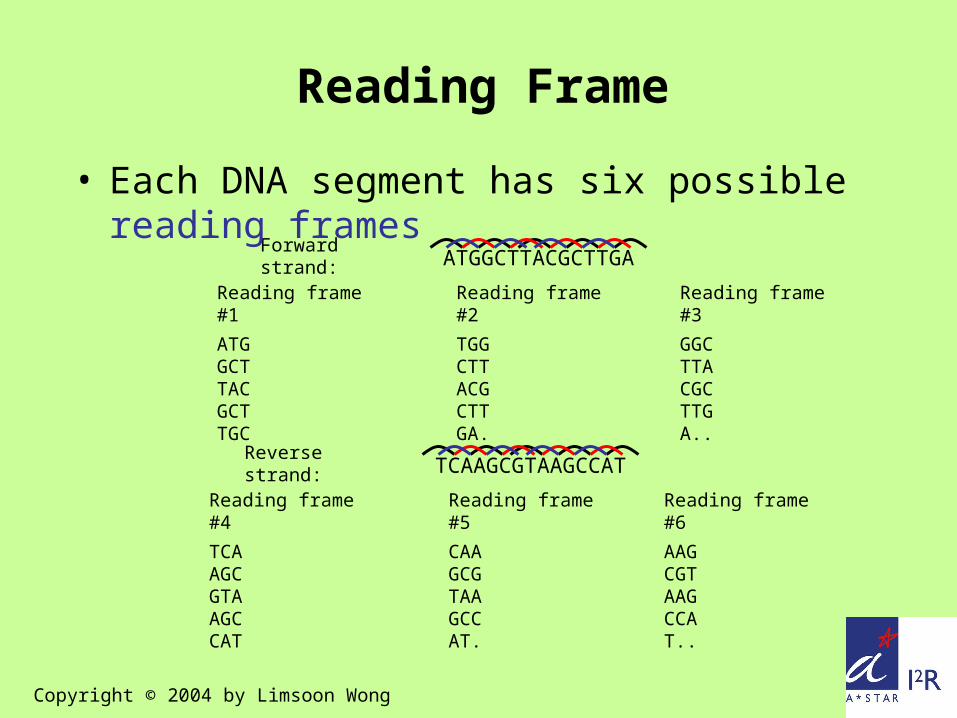
Reading frame #1
ATGGCTTACGCTTGC
Reading frame #2
TGGCTTACGCTTGA.
Reading frame #3
GGCTTACGCTTGA..
ATGGCTTACGCTTGAForward strand:
Reading frame #4
TCAAGCGTAAGCCAT
Reading frame #5
CAAGCGTAAGCCAT.
Reading frame #6
AAGCGTAAGCCAT..
TCAAGCGTAAGCCATReverse strand:
Reading Frame
• Each DNA segment has six possible reading frames
Copyright © 2004 by Limsoon Wong

stop stop
ORF
Open Reading Frame (ORF)
• ORF is a segment of DNA with two in-frame stop codons at the two ends and no in-frame stop codon in the middle
• Each ORF has a fixed reading frame
Copyright © 2004 by Limsoon Wong

Copyright © 2004 by Limsoon Wong
Coding Region
• Each coding region (exon or whole gene) has a fixed translation frame
• A coding region always sits inside an ORF of same reading frame
• All exons of a gene are on the same strand
• Neighboring exons of a gene could have different reading frames
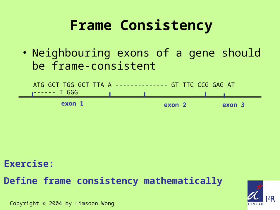
ATG GCT TGG GCT TTA A -------------- GT TTC CCG GAG AT ------ T GGG
exon 1 exon 3exon 2
Frame Consistency
• Neighbouring exons of a gene should be frame-consistent
Copyright © 2004 by Limsoon Wong
Exercise:
Define frame consistency mathematically

Cop
yrig
ht ©
200
4 by
Lim
soon
Won
g
Any Question?

Cop
yrig
ht ©
200
4 by
Lim
soon
Won
g
Overview of Gene Finding
Some slides here are “borrowed” from Mark Craven

What is Gene Finding?
• Find all coding regions from a stretch of DNA sequence, and construct gene structures from the identified exons
• Can be decomposed into– Find coding potential
of a region in a frame– Find boundaries betw
coding & non-coding regions
Copyright © 2004 by Limsoon Wong
Image credit: Xu
Copyright © 2004 by Limsoon Wong
Approaches
• Search-by-signal: find genes by identifying the sequence signals involved in gene expression
• Search-by-content: find genes by statistical properties that distinguish protein coding DNA from non-coding DNA
• Search-by-homology: find genes by homology (after translation) to proteins
• State-of-the-art systems for gene finding usually combine these strategies
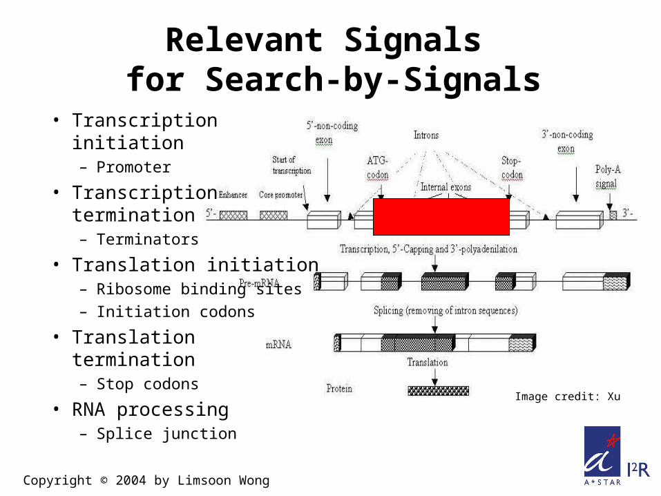
Relevant Signals for Search-by-Signals
• Transcription initiation– Promoter
• Transcription termination– Terminators
• Translation initiation– Ribosome binding sites– Initiation codons
• Translation termination– Stop codons
• RNA processing– Splice junction
Copyright © 2004 by Limsoon Wong
Image credit: Xu

Copyright © 2004 by Limsoon Wong
How Search-by-Signal Works
• There are 2 impt regions in a promoter seq–10 region, ~10bp before TSS–35 region, ~35bp before TSS
• Consensus for–10 region in E. coli is TATAAT, but few promoters actually have this seq
Recognize promoters by– weight matrices– probabilistic models– neural networks, …

How Search-by-Content Works
• Encoding a protein affects stats properties of a DNA seq– some amino acids used
more frequently– diff number of codons
for diff amino acids– for given protein,
usually one codon is used more frequently than others
Estimate prob that a given region of seq was “caused by” its being a coding seq
Copyright © 2004 by Limsoon Wong
Image credit: Craven

Copyright © 2004 by Limsoon Wong
How Search-by-Homology Works
• Translate DNA seq in all reading frames• Search against protein db• High-scoring matches suggest presence
of homologous genes in DNA You can use BLASTX for this

Copyright © 2004 by Limsoon Wong
Search-by-Content Example: Codon Usage Method
• Staden & McLachlan, 1982• Process a seq w/ “window” of length L• Assume seq falls into one of 7 categories,
viz.– Coding in frame 0, frame 1, …, frame 5– Non-coding
• Use Bayes’ rule to determine prob of each category
• Assign seq to category w/ max prob

Image credit: Craven

Image credit: Craven

Image credit: Craven
• Pr(codingi) is the same for each frame if window size fits same number of codons in each frame
• otherwise, consider relative number of codons in window in each frame

Image credit: Craven

Genbank or nr
candidate gene
BLAST search
sequence alignments with known genes,
alignment p-values
Image credit: Xu
Copyright © 2004 by Limsoon Wong
Search-by-Homology Example: Gene Finding Using
BLAST• High seq similarity typically implies
homologous genes Search for genes in yeast seq using
BLAST Extract Feature for gene identification

BLAST hits
sequence
• Searching all ORFs against known genes in nr db helps identify an initial set of (possibly incomplete) genes
Image credit: Xu
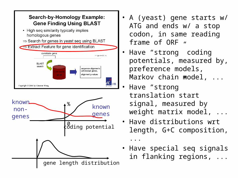
• A (yeast) gene starts w/ ATG and ends w/ a stop codon, in same reading frame of ORF
• Have “strong” coding potentials, measured by, preference models, Markov chain model, ...
• Have “strong” translation start signal, measured by weight matrix model, ...
• Have distributions wrt length, G+C composition, ...
• Have special seq signals in flanking regions, ...
known genes
0
%known non-
genes
coding potential
gene length distribution

Cop
yrig
ht ©
200
4 by
Lim
soon
Won
g
Any Question?
Cop
yrig
ht ©
200
4 by
Lim
soon
Won
g
GRAIL,An Important Gene Finding Program
• Signals assoc w/ coding regions • Models for coding regions• Signals assoc w/ boundaries • Models for boundaries• Other factors & information fusion
Some slides here are “borrowed” from Ying Xu

Coding Signal
• Freq distribution of dimers in protein sequence
• E.g., Shewanella– Ave freq is 5%– Some amino
acids prefer to be next to each other
– Some amino acids prefer to be not next to each other
Copyright © 2004 by Limsoon Wong
Exercise: What is shewanella?
Image credit: Xu

Copyright © 2004 by Limsoon Wong
Coding Signal
• Dimer preference implies dicodon (6-mers like AAA TTT) bias in coding vs non-coding regions
• Relative freq of a di-codon in coding vs non-coding– Freq of dicodon X (e.g, AAA AAA) in coding region, total
number of occurrences of X divided by total number of dicocon occurrences
– Freq of dicodon X (e.g, AAA AAA) in noncoding region, total number of occurrences of X divided by total number of dicodon occurrences
• Exercise: In human genome, freq of dicodon “AAA AAA” is ~1% in coding region vs ~5% in non-coding region. If you see a region with many “AAA AAA”, would you guess it is a coding or non-coding region?

Copyright © 2004 by Limsoon Wong
There are
43 = 64 codons
46 = 4096 dicodons
49 = 262144 tricodons
Why Dicodon (6-mer)?
• Codon (3-mer)-based models are not as info rich as dicodon-based models
• Tricodon (9-mer)-based models need too many data points
• To make stats reliable, need ~15 occurrences of each X-mer
For tricodon-based models, need at least 15*262144 = 3932160 coding bases in our training data, which is probably not going to be available for most genomes

Copyright © 2004 by Limsoon Wong
• Most dicodons show bias towards either coding or non-coding regions
Foundation for coding region identification
Dicodon freq are key signal used for coding region detection; all gene finding programs use this info
Regions consisting of dicodons that mostly tend to be in coding regions are
probably coding regions; otherwise non-coding regions
Coding Signal

Shewanella Bovine
Coding Signal
• Dicodon freq in coding vs non-coding are genome-dependent
Copyright © 2004 by Limsoon Wong
Image credit: Xu
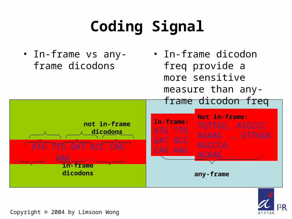
• In-frame vs any-frame dicodons
ATG TTG GAT GCC CAG AAG.....
in-frame dicodons
not in-frame dicodonsIn-frame:
ATG TTGGAT GCCCAG AAG
Not in-frame:
TGTTGG, ATGCCCAGAAG ., GTTGGAAGCCCA, AGAAG ..
any-frame
Coding Signal
• In-frame dicodon freq provide a more sensitive measure than any-frame dicodon freq
Copyright © 2004 by Limsoon Wong
Copyright © 2004 by Limsoon Wong
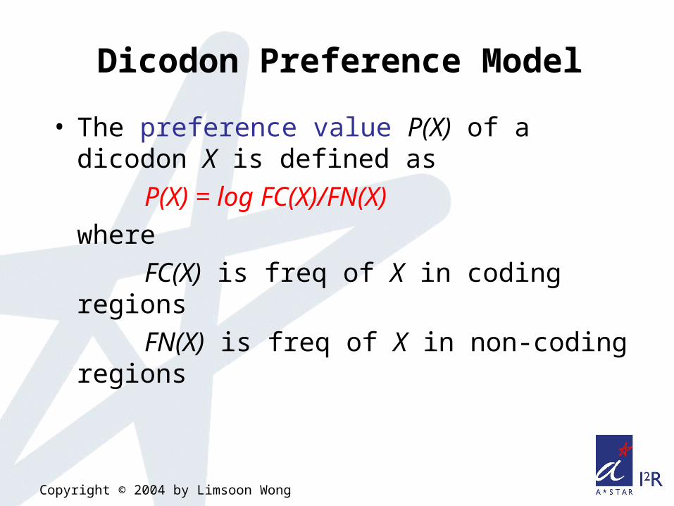
Dicodon Preference Model
• The preference value P(X) of a dicodon X is defined as
P(X) = log FC(X)/FN(X)where
FC(X) is freq of X in coding regionsFN(X) is freq of X in non-coding
regions

Copyright © 2004 by Limsoon Wong
Dicodon Preference Model’s Properties
• P(X) = 0 if X has same freq in coding and non-coding regions
• P(X) > 0 if X has higher freq in coding than in non-coding region; the larger the diff, the more positive the score is
• P(X) < 0 if X has higher freq in non-coding than in coding region; the larger the diff, the more negative the score is

Copyright © 2004 by Limsoon Wong
Dicodon Preference Model Example
• Suppose AAA ATT, AAA GAC, AAA TAG have the following freq:
FC(AAA ATT) = 1.4%FN(AAA ATT) = 5.2%
FC(AAA GAC) = 1.9%FN(AAA GAC) = 4.8%
FC(AAA TAG) = 0.0%FN(AAA TAG) = 6.3%
• ThenP(AAA ATT) = –0.57P(AAA GAC) = –0.40
P(AAA TAG) = –,treating STOP codons
differently
A region consisting of only these dicodons is probably a non-coding region

Copyright © 2004 by Limsoon Wong
Frame-Insensitive Coding Region Preference
Model• A frame-insensitive coding preference
Sis(R) of a region R can be defined as
Sis(R) = X is a dicodon in R P(X)
• R is predicted as coding region if Sis(R) > 0
• NB. This model is not commonly used

Copyright © 2004 by Limsoon Wong
In-Frame Dicodon Preference Model
• The in-frame + i preference value Pi(X) of a dicodon X is defined as
Pi(X) = log FCi(X)/FN(X)
• where FCi(X) is freq of X in coding regions
at in-frame + i positionsFN(X) is freq of X in non-coding
regions ATG TGC CGC GCT P0
P1
P2

Copyright © 2004 by Limsoon Wong
In-Frame Coding Region Preference
Model• The in-frame + i preference Si(R) of a region R
can be defined as
Si(R) = X is a dicodon at in-frame + i position in R Pi(X)
• R is predicted as coding if i=0,1,2 Si(R)/|R| > 0
• NB. This coding preference model is commonly used

• Calculate all ORFs of a DNA segment• For each ORF
– Slide thru ORF w/ increment of 10bp– Calculate in-frame coding region preference
score, in same frame as ORF, within window of 60bp
– Assign score to center of window
• E.g., forward strand in a particular frame...
preference scores
0
+5
-5
Coding Region Prediction: An Example Procedure
Copyright © 2004 by Limsoon Wong
Image credit: Xu

• Making the call: coding or non-coding and where the boundaries are
Need training set with known coding and non-coding regions to select threshold that includes as many known coding regions as possible, and at the same time excludes as many known non-coding regions as possible
coding region? where to draw the
boundaries?
where to draw the line?
Problem with Coding Region Boundaries
Copyright © 2004 by Limsoon Wong
Image credit: Xu

• Knowing boundaries of coding regions helps identify them more accurately
• Possible boundaries of an exon
• Splice junctions:– Donor site: coding region | GT– Acceptor site: CAG | TAG | coding region
• Translation start– in-frame ATG
{ translation start, acceptor site }
{ translation stop, donor site }
Types of Coding Region Boundaries
Copyright © 2004 by Limsoon Wong
Image credit: Xu

Copyright © 2004 by Limsoon Wong
• Splice junction sites and translation starts have certain distribution profiles
• For example, ...
Signals for Coding Region Boundaries

• If we align all known acceptor sites (with their splice junction site aligned), we have the following nucleotide distribution
• Acceptor site: CAG | TAG | coding region
Acceptor Site (Human Genome)
Copyright © 2004 by Limsoon Wong
Image credit: Xu

• If we align all known donor sites (with their splice junction site aligned), we have the following nucleotide distribution
• Donor site: coding region | GT
Donor Site (Human Genome)
Image credit: Xu
Copyright © 2004 by Limsoon Wong

Copyright © 2004 by Limsoon Wong
• For a weight matrix, information content of each column is calculated as
– X{A,C,G,T} F(X)*log (F(X)/0.25)
When a column has evenly distributed nucleotides, its information content is lowest
Only need to look at positions having high information content
What Positions Have “High” Information Content?

• Information contentcolumn –3 = – .34*log (.34/.25) – .363*log
(.363/.25) – .183* log (.183/.25) – .114* log (.114/.25) = 0.04
column –1 = – .092*log (.92/.25) – .03*log (.033/.25) – .803* log (.803/.25) – .073* log (.73/.25) = 0.30
Image credit: Xu
Information Content Around Donor Sites in Human
Genome
Copyright © 2004 by Limsoon Wong

• Weight matrix model – build a weight matrix for donor, acceptor,
translation start site, respectively– use positions of high information content
Weight Matrix Model for Splice Sites
Image credit: Xu
Copyright © 2004 by Limsoon Wong

Copyright © 2004 by Limsoon Wong
• Add up freq of corr letter in corr positions:
• Make prediction on splice site based on some threshold
AAGGTAAGT: .34 + .60 + .80 +1.0 + 1.0 + .52 + .71 + .81 + .46 = 6.24
TGTGTCTCA: .11 + .12 + .03 +1.0 + 1.0 + .02 + .07 + .05 + .16 = 2.56
Image credit: Xu
Splice Site Prediction: A Procedure

Copyright © 2004 by Limsoon Wong
Other Factors Considered by GRAIL
• G+C composition affects dicodon distributions
• Length of exons follows certain distribution• Other signals associated with coding
regions– periodicity – structure information – .....
• Pseudo genes• ........

Info Fusion by ANN in GRAIL
Image credit: Xu
Copyright © 2004 by Limsoon Wong

Copyright © 2004 by Limsoon Wong
Remaining Challenges in GRAIL
• Initial exon • Final exon• Indels & frame shifts

Cop
yrig
ht ©
200
4 by
Lim
soon
Won
g
Any Question?

Cop
yrig
ht ©
200
4 by
Lim
soon
Won
g
Indel & Frame-Shift in Coding Regions
• Problem definition• Indel & frameshift identification• Indel correction• An iterative strategy
Some slides here are “borrowed” from Ying Xu

Copyright © 2004 by Limsoon Wong
• Indel = insertion or deletion in coding region
• Indels are usually caused by seq errorsATG GAT CCA CAT …..
ATG GAT CA CAT …..
ATG GAT CTCA CAT …..
Indels in Coding Regions
Copyright © 2004 by Limsoon Wong

Copyright © 2004 by Limsoon Wong
Effects of Indels on Exon Prediction
• Indels may cause shifts in reading frames & affect prediction algos for coding regions
prefscores
exon
indel
Image credit: Xu

• Preferred reading frame is reading frame w/ highest coding score
• Diff DNA segments may have diff preferred reading frames
Segment a coding sequence into regions w/ consistent preferred reading frames corr well w/ indel positions
Indel identification problem can be solved as a sequence segmentation problem!
Key Idea for Detecting Frame-Shift
Copyright © 2004 by Limsoon Wong
Image credit: Xu

Copyright © 2004 by Limsoon Wong
Frame-Shift Detection by Sequence Segmentation
• Partition seq into segs so that– Chosen frames of adjacent segs are diff– Each segment has >30 bps to avoid small
fluctuations– Sum of coding scores in the chosen frames
over all segments is maximized
• This combinatorial optimization problem can be solved in 6 steps...

Copyright © 2004 by Limsoon Wong
Frame-Shift Detection: Step 1
• Given DNA sequence a1 … an
• Define key quantitiesC(i, r, 1) = max score on a1 … ai,
w/ the last segment in frame r C(i, r, 0) = C(i, r, 1) except that
the last seg may have <30 bps

Copyright © 2004 by Limsoon Wong
Frame-Shift Detection: Step 2
• Determine relationships among the quantities and the optimization problem, viz.
maxr{0, 1, 2}C(i, r, 1) is optimal solution
• Can calculate C(i, r, 0) & C(i, r, 1) from C(i–k, r, 0) & C(i – k, r, 1) for some k > 0

Copyright © 2004 by Limsoon Wong
Frame-Shift Detection: Step 2, C(i,r,0)
• To calculate C(i,r,0), there are 3 possible cases for each position i:– Case 1: no indel occurred at position i
– Case 2: ai is an inserted base
– Case 3: a base has been deleted in front of ai
C(i, r, 0) = max { Case 1, Case 2, Case 3 }

Copyright © 2004 by Limsoon Wong
• No indel occurs at position i. Then
C(i,r,0) = C(i–1,(2+r) mod 3,0) + P(1+r) mod 3 (ai–5…ai)
a1 a2 …… ai-5 ai-4 ai-3 ai-2 ai-1 ai
di-codon preference
Frame-Shift Detection: Step 2, Case 1

Copyright © 2004 by Limsoon Wong
a1 a2 …… ai-6 ai-5 ai-4 ai-3 ai-2 ai-1 ai
di-codon preference
Frame-Shift Detection: Step 2, Case 2
• ai-1 is an inserted base. Then
C(i,r,0) = C(i–2, (r+2) mod 3, 1) + P(1+r) mod 3 (ai–6...a i–2ai)

Copyright © 2004 by Limsoon Wong
a1 a2 …… ai-5 ai-4 ai-3 ai-2 ai-1 ai
add a neutral base “C”
Frame-Shift Detection: Step 2, Case 3
• A base has been deleted in front of ai. Then
C(i, r, 0) = C(i–1, (r+1) mod 3, 1) + Pr (ai–5… ai–1C) +
P(1+r) mod 3 (ai–4… ai–1Cai)

Copyright © 2004 by Limsoon Wong
C(i, r, 1) = C(i–30, r, 0) +
i–30 < j i–5 P(j+r) mod 3 (aj…aj+5)
a1 a2 …… ai-30 ai-30+1 …… ai
summed di-codon preference
coding score in frame r
Frame-Shift Detection: Step 2, C(i,r,1)
• To calculate C(i,r,1),
Exercise:This formula is not quite right. Fix it.

Copyright © 2004 by Limsoon Wong
Frame-Shift Detection: Step 2, Initiation
• Initial conditions,C (k, r, 0) = –, k < 6C (6, r, 0) = P(1+r) mod 3 (a1 … a6)
C(i, r, 1) = –, i < 30
• This is a dynamic programming (DP) algorithm; the equations are DP recurrences

Frame-Shift Detection: Step 3
• Calculation of maxr{0, 1, 2}C(i, r, 1) gives an optimal segmentation of a DNA sequence
• Tracing back the transition points---viz. case 2 & case 3---gives the segmentation results
frame 0 frame 1 frame 2
Copyright © 2004 by Limsoon Wong
Image credit: Xu

Frame-Shift Detection: Step 4• Determine of coding regions
– For given H1 and H2 (e.g., = 0.25 and 0.75), partition a DNA seq into segs so that each seg has >30 bases & coding values of each seg are consistently closer to one of H1 or H2 than the other
H1
H2
segmentation result
Copyright © 2004 by Limsoon Wong
Image credit: Xu

Frame-Shift Detection: Step 5
• Overlay “preferred reading-frame segs” & “coding segs” gives coding region predictions regions w/ indels
Copyright © 2004 by Limsoon Wong
Image credit: Xu

Copyright © 2004 by Limsoon Wong
• If an “insertion” is detected, delete the base at the transition point
• If a “deletion” is detected, add a neutral base “C” at transition point
Frame-Shift Detection: Step 6
• We still need to correct the identified indels...
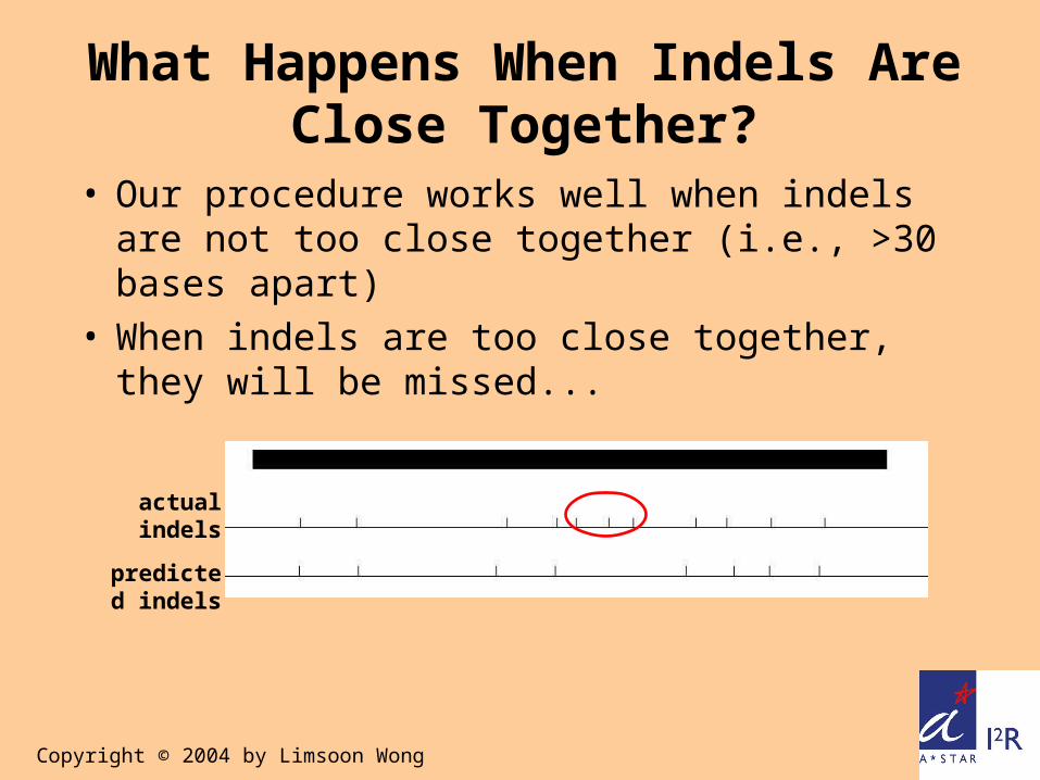
actual indels
predicted indels
What Happens When Indels Are Close Together?
• Our procedure works well when indels are not too close together (i.e., >30 bases apart)
• When indels are too close together, they will be missed...
Copyright © 2004 by Limsoon Wong
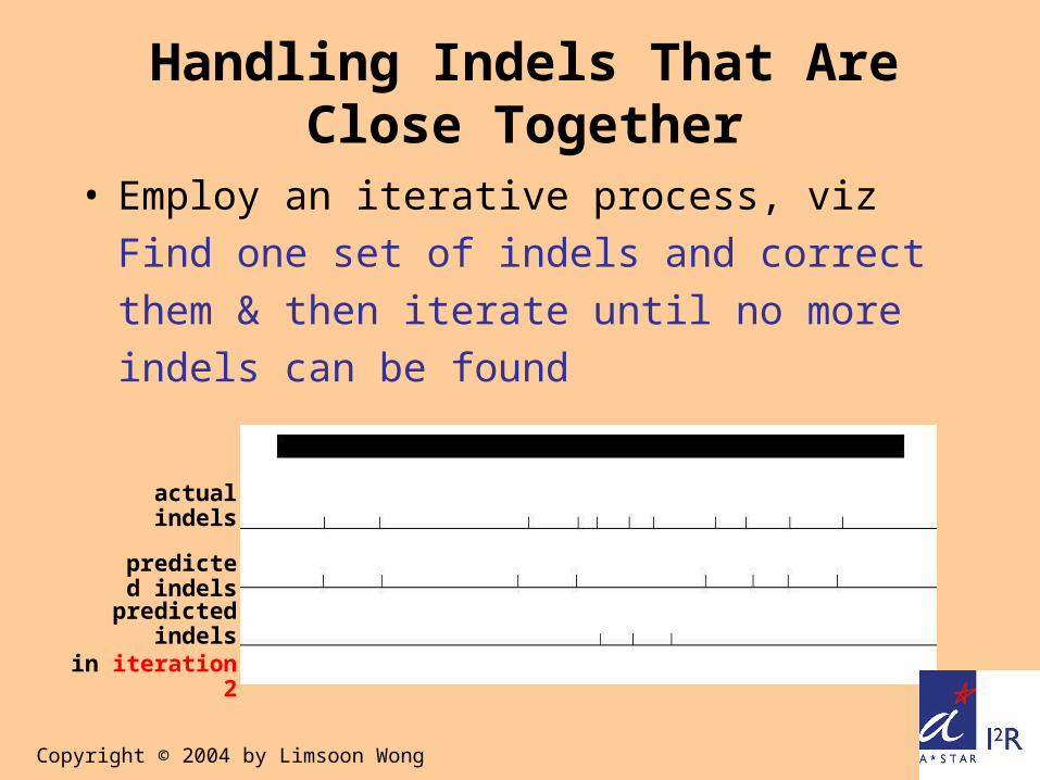
• Employ an iterative process, vizFind one set of indels and correct them & then iterate until no more indels can be found
actual indels
predicted indels
predicted indelsin iteration 2
Handling Indels That Are Close Together
Copyright © 2004 by Limsoon Wong

Cop
yrig
ht ©
200
4 by
Lim
soon
Won
g
Any Question?

Cop
yrig
ht ©
200
4 by
Lim
soon
Won
g
Modeling & Recognition of
Histone Promoters
Some slides here are “borrowed” from Rajesh Chowdhary
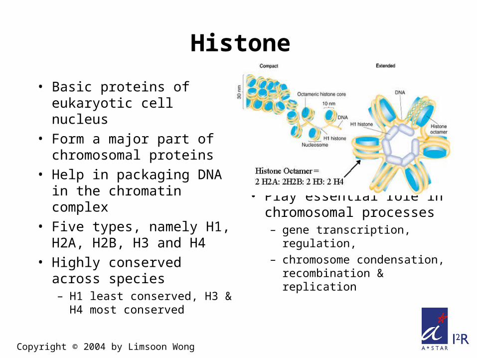
• Play essential role in chromosomal processes– gene transcription,
regulation, – chromosome
condensation, recombination & replication
Copyright © 2004 by Limsoon Wong
Histone
• Basic proteins of eukaryotic cell nucleus
• Form a major part of chromosomal proteins
• Help in packaging DNA in the chromatin complex
• Five types, namely H1, H2A, H2B, H3 and H4
• Highly conserved across species– H1 least conserved, H3
& H4 most conserved

Histone Transcription• TFs bound in core,
proximal, distal promoter & enhancer regions
• TFIID binds to TATA box & identifies TSS with help of TAFs & TBP
• RNA Pol-II supplemented by GTFs (A,B,D,E,F,H) recruited to core promoter to form Pre-initiation complex
• Transcription initiated– Basal/Activated, depending
on space & time
Copyright © 2004 by Limsoon Wong

Histone Promoter ModelingWerner 1999
• Three promoter types: Core, proximal and distal• Characterised by the presence of specific TFBSs
– CAAT box, TATA Box, Inr, & DPE– Order and mutual distance of TFBS modules is specific
& determine function
Copyright © 2004 by Limsoon Wong

Histone H1t Gene RegulationGrimes et al. 2003
• One gene can express in diff ways in diff cells
• Same binding site can have diff functions in diff cells
Copyright © 2004 by Limsoon Wong

Copyright © 2004 by Limsoon Wong
Why Model Histone promoters
• To understand histone’s regulatory mechanism – To characterise regulatory features from
known promoters– To identify promoter from uncharacterised
genomic sequence (promoter recognition)– To find other genes with similar regulatory
behaviour and gene-products – To define potential gene regulatory networks

Copyright © 2004 by Limsoon Wong
Difficulties of Histone Promoter Modeling
• Not a plain sequence alignment problem• Not all features are common among
different groups• Not only TFBSs’ presence, but their
location, order, mutual distance and orientation are critical to promoter function
• Not all TFs & TFBSs have been characterized yet
Copyright © 2004 by Limsoon Wong
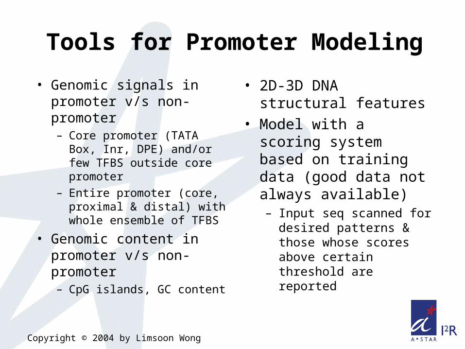
Tools for Promoter Modeling
• Genomic signals in promoter v/s non-promoter– Core promoter (TATA
Box, Inr, DPE) and/or few TFBS outside core promoter
– Entire promoter (core, proximal & distal) with whole ensemble of TFBS
• Genomic content in promoter v/s non-promoter – CpG islands, GC content
• 2D-3D DNA structural features
• Model with a scoring system based on training data (good data not always available)– Input seq scanned for
desired patterns & those whose scores above certain threshold are reported

Promoter Recognition Programs
• Programs have different objectives
• Use various combinations of genomic signals and content
• Typically analyse 5’ region [-1000,+500]
• Due to low accuracy, programs developed for sub-classes of promoters
Copyright © 2004 by Limsoon Wong
Image credit: Rajesh

Copyright © 2004 by Limsoon Wong
Steps for Building Histone Promoter Recognizer
• Exercise: What do you think these steps are?
Copyright © 2004 by Limsoon Wong
MEME
• MEME is a powerful and good method for finding motifs from biological sequences
• T. L. Bailey & C. Elkan, "Fitting a mixture model by expectation maximization to discover motifs in
biopolymers", ISMB, 2:28--36, 1994

H2A
Motifs Discovered by MEME in Histone Gene 5’ Region [-
1000,+500]
Copyright © 2004 by Limsoon Wong
Image credit: Rajesh

H2B
Motifs Discovered by MEME in Histone Gene 5’ Region [-
1000,+500]
Copyright © 2004 by Limsoon Wong
Image credit: Rajesh

Are These Really Motifs of H2A and H2B Promoters?
Copyright © 2004 by Limsoon Wong
H2B
H2A
• One could use the motifs discovered by MEME to detect H2A & H2B promoters
• But….it is strange that the motifs for H2A and H2B are generally the same, but in opposite orientation
• Exercise: Suggest a possible explanation Image credit: Rajesh

The Real Common Promoter Region of H2A & H2B is at [-
250,-1]!
Copyright © 2004 by Limsoon Wong
H2B
H2A
• MEME was overwhelmed by coding region & did not find the right motifs! Image credit: Rajesh
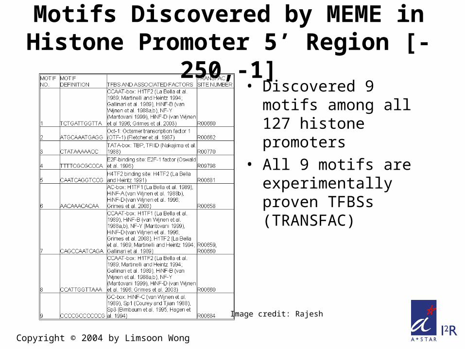
Motifs Discovered by MEME in Histone Promoter 5’ Region [-
250,-1]• Discovered 9 motifs
among all 127 histone promoters
• All 9 motifs are experimentally proven TFBSs (TRANSFAC)
Copyright © 2004 by Limsoon Wong
Image credit: Rajesh

Deriving Histone Promoter Models
• Divide H1 seqs into 5 subgroups
• Aligned seqs within each subgroup
• Consensus alignment matches biologically known H1 subgroup models
Can apply same approach to find promoter models for H2A, H2B, H3, H4...
Copyright © 2004 by Limsoon Wong
Image credit: Rajesh

Cop
yrig
ht ©
200
4 by
Lim
soon
Won
g
Any Question?

Cop
yrig
ht ©
200
4 by
Lim
soon
Won
g
Knowledge Discovery Basics
• Knowledge discovery in brief• K-Nearest Neighbour• Support Vector Machines• Bayesian Approach• Hidden Markov Models• Artificial Neural Networks Some slides are from a tutorial jointly taught with Jinyan Li
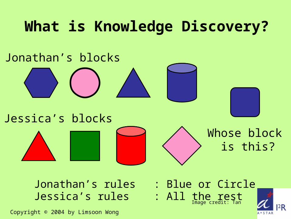
Jonathan’s rules : Blue or CircleJessica’s rules : All the rest
Whose block is this?
Jonathan’s blocks
Jessica’s blocks
What is Knowledge Discovery?
Copyright © 2004 by Limsoon Wong
Image credit: Tan
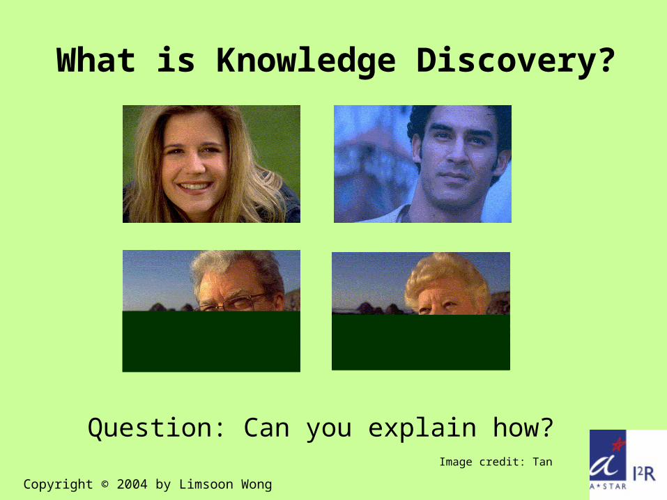
Question: Can you explain how?
What is Knowledge Discovery?
Copyright © 2004 by Limsoon Wong
Image credit: Tan

Copyright © 2004 by Limsoon Wong
Some classifiers/learning methods
Steps of Knowledge Discovery
• Training data gathering• Feature generation
– k-grams, colour, texture, domain know-how, ...
• Feature selection– Entropy, 2, CFS, t-test, domain know-how...
• Feature integration– SVM, ANN, PCL, CART, C4.5, kNN, ...

Copyright © 2004 by Limsoon Wong
Some Knowledge Discovery Methods
• K-Nearest Neighbour• Support Vector Machines• Bayesian Approach• Hidden Markov Models• Artificial Neural Networks

Copyright © 2004 by Limsoon Wong
• A common “distance” measure betw samples x and y is
where f ranges over features of the samples
How kNN Works
• Given a new case• Find k “nearest”
neighbours, i.e., k most similar points in the training data set
• Assign new case to the same class to which most of these neighbours belong

Neighborhood
5 of class
3 of class
=
Illustration of kNN (k=8)
Copyright © 2004 by Limsoon Wong
Image credit: Zaki

Enzyme inducers
Peroxisome proliferators
Copyright © 2004 by Limsoon Wong
Prediction of Compound Signature Based on Gene
Expression Profiles• Hamadeh et al, Toxicological
Sciences 67:232-240, 2002
• Store gene expression profiles corr to biological responses to exposures to known compounds whose toxicological and pathological endpoints are well characterized
• use kNN to infer effects of unknown compound based on gene expr profiles induced by it
Copyright © 2004 by Limsoon Wong
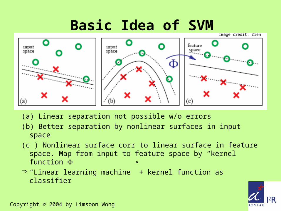
(a) Linear separation not possible w/o errors(b) Better separation by nonlinear surfaces in input space(c ) Nonlinear surface corr to linear surface in feature
space. Map from input to feature space by “kernel” function
“Linear learning machine” + kernel function as classifier
Basic Idea of SVMImage credit: Zien

• Hyperplane separating the x’s and o’s points is given by (W•X) + b = 0, with (W•X) = jW[j]*X[j]
Decision function is llm(X) = sign((W•X) + b))
Linear Learning Machines
Copyright © 2004 by Limsoon Wong

Copyright © 2004 by Limsoon Wong
• Solution is a linear combination of training points Xk with labels Yk
W[j] = kk*Yk*Xk[j],
with k > 0, and Yk = ±1
llm(X) = sign(kk*Yk* (Xk•X) + b)
Linear Learning Machines
“data” appears only in dot product!

• llm(X) = sign(kk*Yk* (Xk•X) + b)
• svm(X) = sign(kk*Yk* (Xk• X) + b)
svm(X) = sign(kk*Yk* K(Xk,X) + b)
where K(Xk,X) = (Xk• X)
Kernel Function
Copyright © 2004 by Limsoon Wong

Copyright © 2004 by Limsoon Wong
Kernel Function
• svm(X) = sign(kk*Yk* K(Xk,X) + b) K(A,B) can be computed w/o computing
• In fact replace it w/ lots of more
“powerful” kernels besides (A • B). E.g.,– K(A,B) = (A • B)d
– K(A,B) = exp(– || A B||2 / (2*)), ...

Copyright © 2004 by Limsoon Wong
How SVM Works
• svm(X) = sign(kk*Yk* K(Xk,X) + b)
• To find k is a quadratic programming problem
max: kk – 0.5 * k h k*h Yk*Yh*K(Xk,Xh)
subject to: kk*Yk=0
and for all k , C k 0
• To find b, estimate by averagingYh – kk*Yk* K(Xh,Xk)
for all h 0

Prediction of Gene Function From Gene Expression Data
Using SVM• Brown et al., PNAS
91:262-267, 2000
• Use SVM to identify sets of genes w/ a c’mon function based on their expression profiles
• Use SVM to predict functional roles of uncharacterized yeast ORFs based on their expression profiles
Copyright © 2004 by Limsoon Wong

Copyright © 2004 by Limsoon Wong
Bayes Theorem
• P(h) = prior prob that hypothesis h holds• P(d|h) = prob of observing data d given h holds• P(h|d) = posterior prob that h holds given
observed data d
Copyright © 2004 by Limsoon Wong
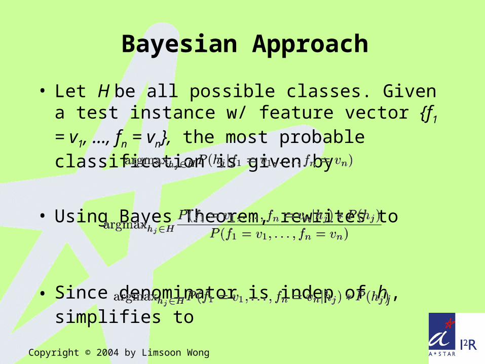
• Let H be all possible classes. Given a test instance w/ feature vector {f1 = v1, …, fn = vn}, the most probable classification is given by
• Using Bayes Theorem, rewrites to
• Since denominator is indep of hj, simplifies to
Bayesian Approach

Copyright © 2004 by Limsoon Wong
Naïve Bayes
• But estimating P(f1=v1, …, fn=vn|hj) accurately may not be feasible unless training data set is sufficiently large
• “Solved” by assuming f1, …, fn are indep
• Then
• where P(hj) and P(fi=vi|hj) can often be estimated reliably from typical training data set

Bayesian Design of Screens for Macromolecular
Crystallization• Hennessy et al., Acta Cryst
D56:817-827, 2000
• Xtallization of proteins requires search of expt settings to find right conditions for diffraction-quality xtals
• BMCD is a db of known xtallization conditions
• Use Bayes to determine prob of success of a set of expt conditions based on BMCD
Copyright © 2004 by Limsoon Wong

How HMM Works
• HMM is a stochastic generative model for sequences
• Defined by– finite set of states S– finite alphabet A– transition prob matrix T– emission prob matrix E
• Move from state to state according to T while emitting symbols according to E
sk
s1
…
s2
a1
a2
Copyright © 2004 by Limsoon Wong

Copyright © 2004 by Limsoon Wong
• In nth order HMM, T & E depend on all n previous states
• E.g., for 1st order HMM, given emissions X = x1, x2, …, & states S = s1, s2, …, the prob of this seq is
• If seq of emissions X is given, use Viterbi algo to get seq of states S such that
S = argmaxS Prob(X, S)
• If emissions unknown, use Baum-Welch algo
How HMM Works

Copyright © 2004 by Limsoon Wong
• Game:– You bet $1– You roll – Casino rolls – Highest number wins
$2
• Question: Suppose we played 2 games, and the sequence of rolls was 1, 6, 2, 6. Were we likely to be cheated?
Example: Dishonest Casino
• Casino has two dices:– Fair dice
• P(i) = 1/6, i = 1..6
– Loaded dice• P(i) = 1/10, i = 1..5• P(i) = 1/2, i = 6
• Casino switches betw fair & loaded die with prob 1/2. Initially, dice is always fair

“Visualization” of Dishonest Casino
Copyright © 2004 by Limsoon Wong

Copyright © 2004 by Limsoon Wong
1, 6, 2, 6? We were probably cheated...

Protein Families Modelling By HMM
• Baldi et al., PNAS 91:1059-1063, 1994
• HMM is used to model families of biological sequences, such as kinases, globins, & immunoglobulins
• Bateman et al., NAR 32:D138-D141, 2004
• HMM is used to model 6190 families of protein domains in Pfam
Copyright © 2004 by Limsoon Wong

What are ANNs?
• ANNs are highly connected networks of “neural computing elements” that have ability to respond to input stimuli and learn to adapt to the environment...
Copyright © 2004 by Limsoon Wong

Computing Element
• Behaves as a monotone function y = f(net), where net is cummulative input stimuli to the neuron
• net is usually defined as weighted sum of inputs
• f is usually a sigmoid
Copyright © 2004 by Limsoon Wong

How ANN Works
• Computing elements are connected into layers in a network
• The network is used for classification as follows:– Inputs xi are fed into
input layer– each computing element
produces its corr output– which are fed as inputs
to next layer, and so on– until outputs are
produced at output layer
• What makes ANN works is how the weights on the links are learned
• Usually achieved using “back propagation”
Copyright © 2004 by Limsoon Wong

vij
wjzj
Back Propagation• vji = weight on link
betw xi and jth computing element in 1st layer
• wj be weight of link betw jth computing element in 1st layer and computing element in last layer
• zj = output of jth computing element in 1st layer
• Then
Copyright © 2004 by Limsoon Wong

Back Propagation
• For given sample, y may differ from target output t by amt
• Need to propagate this error backwards by adjusting weights in proportion to the error gradient
• For math convenience, define the squared error as
To find an expression for weight adjustment, we differentiate E wrt vij and wj to obtain error gradients for these weightsvij
wjzj
Copyright © 2004 by Limsoon Wong

Copyright © 2004 by Limsoon Wong
Applying chain rule a few times and recalling definitions of y, zj, E, and f, we derive...

Back Propagation
vij
wjzj
Copyright © 2004 by Limsoon Wong

T-Cell Epitopes Prediction By ANN
• Honeyman et al., Nature Biotechnology 16:966-969, 1998
• Use ANN to predict candidate T-cell epitopes
Copyright © 2004 by Limsoon Wong
Image credit: Brusic

Cop
yrig
ht ©
200
4 by
Lim
soon
Won
g
Any Question?

Cop
yrig
ht ©
200
4 by
Lim
soon
Won
g
Translation Initiation Site Recognition
An introduction to the World’s simplest TIS recognition system

Translation Initiation Site
Copyright © 2004 by Limsoon Wong

Copyright © 2004 by Limsoon Wong
299 HSU27655.1 CAT U27655 Homo sapiensCGTGTGTGCAGCAGCCTGCAGCTGCCCCAAGCCATGGCTGAACACTGACTCCCAGCTGTG 80CCCAGGGCTTCAAAGACTTCTCAGCTTCGAGCATGGCTTTTGGCTGTCAGGGCAGCTGTA 160GGAGGCAGATGAGAAGAGGGAGATGGCCTTGGAGGAAGGGAAGGGGCCTGGTGCCGAGGA 240CCTCTCCTGGCCAGGAGCTTCCTCCAGGACAAGACCTTCCACCCAACAAGGACTCCCCT............................................................ 80................................iEEEEEEEEEEEEEEEEEEEEEEEEEEE 160EEEEEEEEEEEEEEEEEEEEEEEEEEEEEEEEEEEEEEEEEEEEEEEEEEEEEEEEEEEE 240EEEEEEEEEEEEEEEEEEEEEEEEEEEEEEEEEEEEEEEEEEEEEEEEEEEEEEEEEEE
A Sample cDNA
• What makes the second ATG the TIS?

Copyright © 2004 by Limsoon Wong
Approach
• Training data gathering• Signal generation
– k-grams, distance, domain know-how, ...
• Signal selection– Entropy, 2, CFS, t-test, domain know-how...
• Signal integration– SVM, ANN, PCL, CART, C4.5, kNN, ...

Copyright © 2004 by Limsoon Wong
Training & Testing Data
• Vertebrate dataset of Pedersen & Nielsen [ISMB’97]
• 3312 sequences• 13503 ATG sites• 3312 (24.5%) are TIS• 10191 (75.5%) are non-TIS• Use for 3-fold x-validation expts

Copyright © 2004 by Limsoon Wong
Signal Generation
• K-grams (ie., k consecutive letters)– K = 1, 2, 3, 4, 5, …– Window size vs. fixed position– Up-stream, downstream vs. any where in window– In-frame vs. any frame
0
0.5
1
1.5
2
2.5
3
A C G T
seq1
seq2
seq3

Copyright © 2004 by Limsoon Wong
299 HSU27655.1 CAT U27655 Homo sapiensCGTGTGTGCAGCAGCCTGCAGCTGCCCCAAGCCATGGCTGAACACTGACTCCCAGCTGTG 80CCCAGGGCTTCAAAGACTTCTCAGCTTCGAGCATGGCTTTTGGCTGTCAGGGCAGCTGTA 160GGAGGCAGATGAGAAGAGGGAGATGGCCTTGGAGGAAGGGAAGGGGCCTGGTGCCGAGGA 240CCTCTCCTGGCCAGGAGCTTCCTCCAGGACAAGACCTTCCACCCAACAAGGACTCCCCT
Signal Generation: An Example
• Window = 100 bases• In-frame, downstream
– GCT = 1, TTT = 1, ATG = 1…
• Any-frame, downstream– GCT = 3, TTT = 2, ATG = 2…
• In-frame, upstream– GCT = 2, TTT = 0, ATG = 0, ...

Copyright © 2004 by Limsoon Wong
Too Many Signals
• For each value of k, there are4k * 3 * 2 k-grams
• If we use k = 1, 2, 3, 4, 5, we have4 + 24 + 96 + 384 + 1536 + 6144
= 8188features!
• This is too many for most machine learning algorithms

Signal Selection (Basic Idea)
• Choose a signal w/ low intra-class dist
• Choose a signal w/ high inter-class dist
Copyright © 2004 by Limsoon Wong
Image credit: Slonim

Copyright © 2004 by Limsoon Wong
Signal Selection (eg., t-statistics)

Copyright © 2004 by Limsoon Wong
Signal Selection (eg., 2)

Copyright © 2004 by Limsoon Wong
Signal Selection (eg., CFS)
• Instead of scoring individual signals, how about scoring a group of signals as a whole?
• CFS– Correlation-based Feature Selection– A good group contains signals that are highly
correlated with the class, and yet uncorrelated with each other
Copyright © 2004 by Limsoon Wong
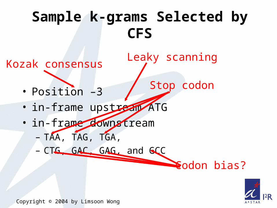
• Position –3• in-frame upstream ATG• in-frame downstream
– TAA, TAG, TGA, – CTG, GAC, GAG, and GCC
Kozak consensusLeaky scanning
Stop codon
Codon bias?
Sample k-grams Selected by CFS
Copyright © 2004 by Limsoon Wong
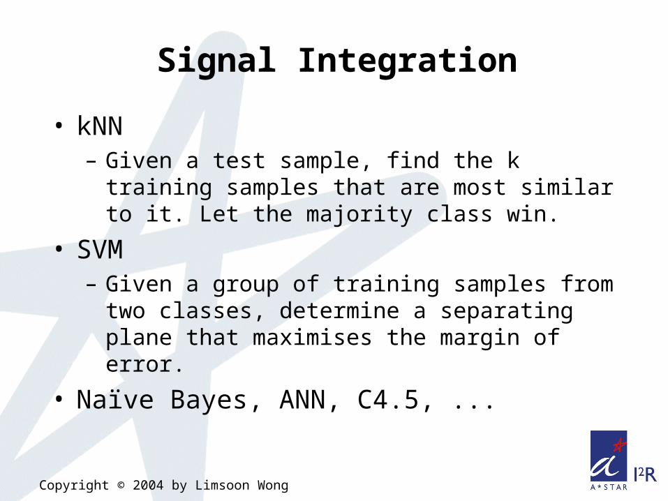
Signal Integration
• kNN– Given a test sample, find the k training
samples that are most similar to it. Let the majority class win.
• SVM– Given a group of training samples from two
classes, determine a separating plane that maximises the margin of error.
• Naïve Bayes, ANN, C4.5, ...
Copyright © 2004 by Limsoon Wong
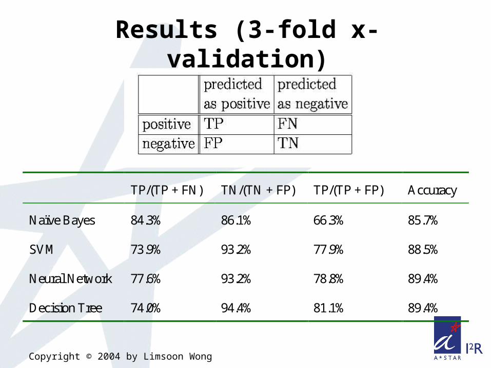
TP/(TP + FN) TN/(TN + FP) TP/(TP + FP) Accuracy
Naïve Bayes 84.3% 86.1% 66.3% 85.7%
SVM 73.9% 93.2% 77.9% 88.5%
Neural Network 77.6% 93.2% 78.8% 89.4%
Decision Tree 74.0% 94.4% 81.1% 89.4%
Results (3-fold x-validation)

Copyright © 2004 by Limsoon Wong
TP/(TP + FN) TN/(TN + FP) TP/(TP + FP) Accuracy
NB 84.3% 86.1% 66.3% 85.7%
SVM 73.9% 93.2% 77.9% 88.5%
NB+Scanning 87.3% 96.1% 87.9% 93.9%
SVM+Scanning 88.5% 96.3% 88.6% 94.4%
Improvement by Scanning
• Apply Naïve Bayes or SVM left-to-right until first ATG predicted as positive. That’s the TIS.
• Naïve Bayes & SVM models were trained using TIS vs. Up-stream ATG
Copyright © 2004 by Limsoon Wong
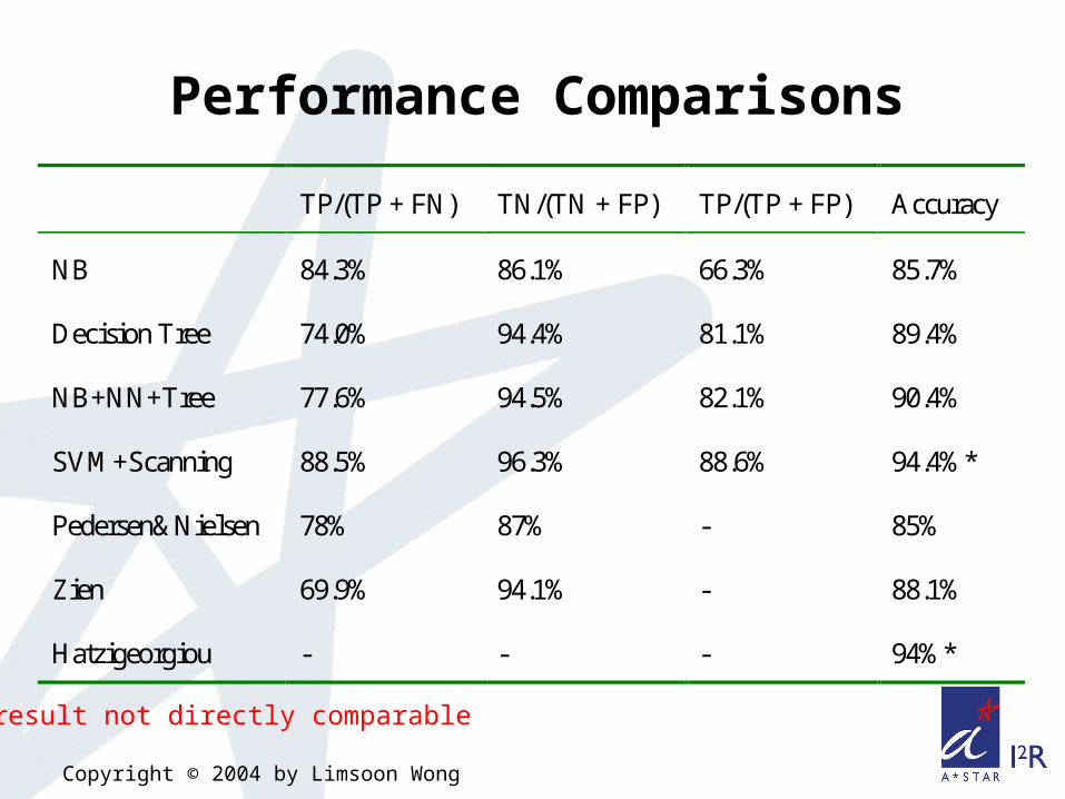
TP/(TP + FN) TN/(TN + FP) TP/(TP + FP) Accuracy
NB 84.3% 86.1% 66.3% 85.7%
Decision Tree 74.0% 94.4% 81.1% 89.4%
NB+NN+Tree 77.6% 94.5% 82.1% 90.4%
SVM+Scanning 88.5% 96.3% 88.6% 94.4%*
Pedersen&Nielsen 78% 87% - 85%
Zien 69.9% 94.1% - 88.1%
Hatzigeorgiou - - - 94%*
* result not directly comparable
Performance Comparisons

F
L
I
MV
S
P
T
A
Y
H
Q
N
K
D
E
C
WR
G
A
T
E
L
R
S
stop
How about using k-grams from the translation?
mRNAprotein
Copyright © 2004 by Limsoon Wong

Amino-Acid Features
Copyright © 2004 by Limsoon WongImage credit: Liu
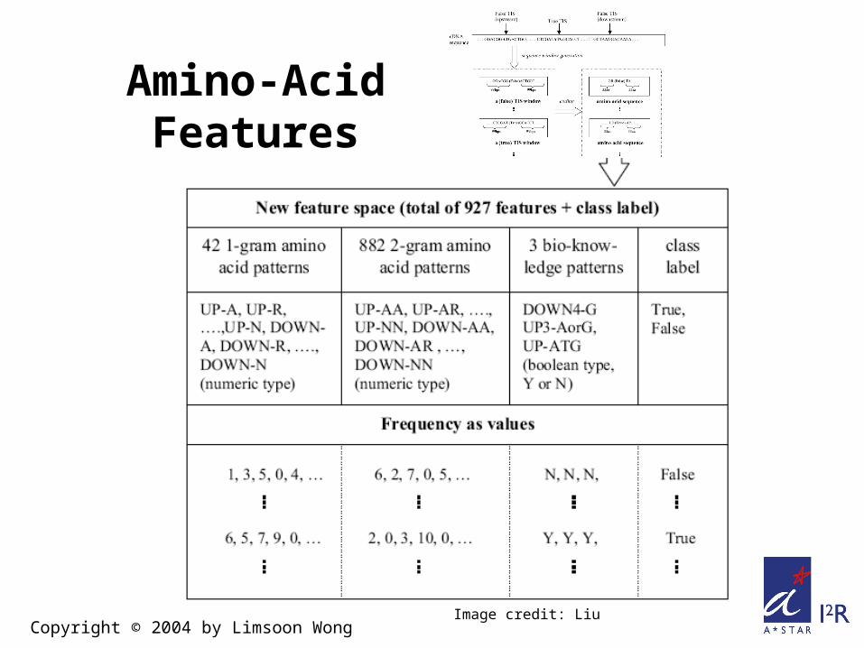
Amino-Acid Features
Copyright © 2004 by Limsoon WongImage credit: Liu

Copyright © 2004 by Limsoon Wong
Amino Acid K-grams Discovered (by entropy)

Copyright © 2004 by Limsoon Wong
Independent Validation Sets
• A. Hatzigeorgiou:– 480 fully sequenced human cDNAs– 188 left after eliminating sequences similar to
training set (Pedersen & Nielsen’s)– 3.42% of ATGs are TIS
• Our own:– well characterized human gene sequences
from chromosome X (565 TIS) and chromosome 21 (180 TIS)

Validation Results (on Hatzigeorgiou’s)
• Using top 100 features selected by entropy and trained on Pedersen & Nielsen’s dataset
Copyright © 2004 by Limsoon Wong

ATGpr
Ourmethod
Validation Results (on Chr X & Chr 21)
• Using top 100 features selected by entropy and trained on Pedersen & Nielsen’s
Copyright © 2004 by Limsoon Wong
Image credit: Liu

Cop
yrig
ht ©
200
4 by
Lim
soon
Won
g
Any Question?
Cop
yrig
ht ©
200
4 by
Lim
soon
Won
g
Human Polyadenylation Signal Prediction
Some slides are “borrowed” from Huiqing Liu

Copyright © 2004 by Limsoon Wong
Cleavage & Polyadenylation of Pre-mRNAs in Mammalian
Cells
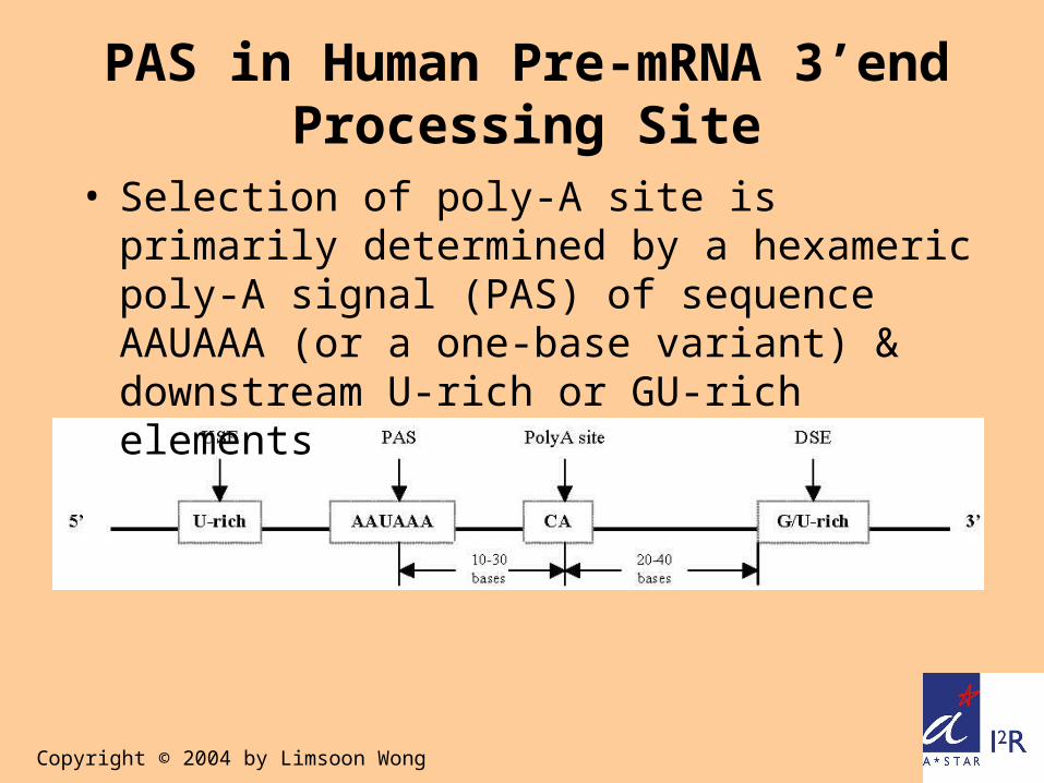
PAS in Human Pre-mRNA 3’end Processing Site
• Selection of poly-A site is primarily determined by a hexameric poly-A signal (PAS) of sequence AAUAAA (or a one-base variant) & downstream U-rich or GU-rich elements
Copyright © 2004 by Limsoon Wong
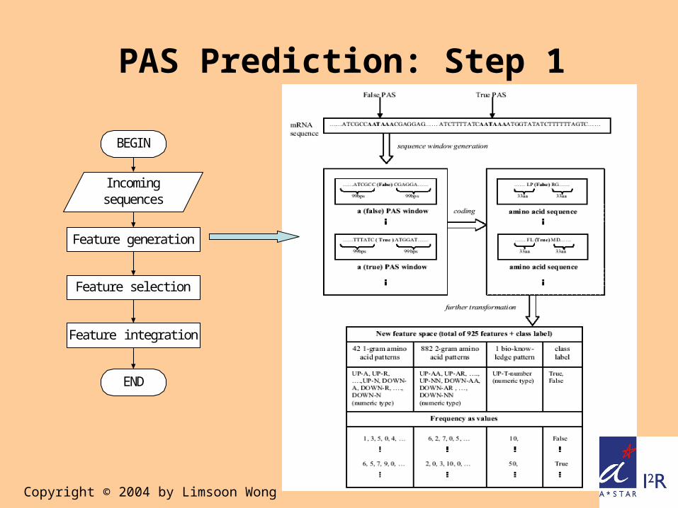
PAS Prediction: Step 1
Feature generati on
I ncomi ngsequences
Feature sel ecti on
Feature i ntegrati on
END
BEGI N
Copyright © 2004 by Limsoon Wong

PAS Prediction: Step 2
discard all the features without cut points.
Entropy Measure for Feature Selection
Fayyad & Irani, IJCAI, 1993
Feature generati on
I ncomi ngsequences
Feature sel ecti on
Feature i ntegrati on
END
BEGI N
Copyright © 2004 by Limsoon Wong

PAS Prediction: Step 3
Copyright © 2004 by Limsoon Wong
SVM in Weka
Feature generati on
I ncomi ngsequences
Feature sel ecti on
Feature i ntegrati on
END
BEGI N

Copyright © 2004 by Limsoon Wong
Data Set I (From Erpin)
• Training set: 2327 seqs– 1632 “unique” & 695
“strong” poly(A) sites
• All seq trimmed to contain 206 bases, having a false or true PAS in the center
• Positive testing set: – 982 seq w/ annotated
PASes from EMBL
• Negative testing set:– 982 CDS seqs– 982 seqs of 1st intron– 982 randomized UTR
seqs using same 1st order Markov model as human 3’ UTRs
– 982 randomized UTR seqs of same mono nucleotide composition as human 3’ UTRs

Copyright © 2004 by Limsoon Wong
Data Set II (mRNA data)
• Positive set: – 312 human mRNA seqs
from RefSeq release 1– Each contains a
“poly(A)-signal” feature tag carrying an “evidence=experimental” label
– 767 human mRNA sequences from RefSeq containing a “poly(A)-site” feature tag carrying an “evidence=experimental” label. Similar sequences have been removed
• Negative set: – Generated by scanning
“AATAAA” at coding region (exclude those near the end of seq)

Experimental Results
• Preliminary test: In order to compare with the performance of Erpin and Polyadq, we also adjust prediction accuracy on 982 true PASes at around 56%.
Copyright © 2004 by Limsoon Wong

All the numbers regarding to the performance of Erpin and Polyadq are copied or derived from Legendre & Gautheret 2003
Experimental Results
• Testing results on Erpin using validation sets
Copyright © 2004 by Limsoon Wong

It is clear that both upstream and dowstream are well-characterized by G/U rich segments (consistent w/ reported motifs)
Experimental Results
• Top ranked features
Copyright © 2004 by Limsoon Wong

Cop
yrig
ht ©
200
4 by
Lim
soon
Won
g
Any Question?

Cop
yrig
ht ©
200
4 by
Lim
soon
Won
g
Recognition of Transcription Start
Sites
An introduction to the World’s best TSS
recognition system: A heavy tuning approach

Copyright © 2004 by Limsoon Wong
Transcription Start Site

Copyright © 2004 by Limsoon Wong
-200 to +50window size
Model selected based on desired sensitivity
Structure of Dragon Promoter Finder
Image credit: Bajic

GC-rich submodel
GC-poor submodel
(C+G) =#C + #GWindow Size
Copyright © 2004 by Limsoon Wong
Each model has two submodels based on GC
content
Image credit: Bajic

K-gram (k = 5) positional weight matrix
p
e
i
Data Analysis Within Submodel
Copyright © 2004 by Limsoon WongImage credit: Bajic

Pentamer at ith
position in input
jth pentamer atith position in training window
Frequency of jthpentamer at ith positionin training window
Window size
Promoter, Exon, Intron Sensors
• These sensors are positional weight matrices of k-grams, k = 5 (aka pentamers)
• They are calculated as s below using promoter, exon, intron data respectively
Copyright © 2004 by Limsoon Wong

Tuning parameters
tanh(x) =ex e-x
ex e-x
sIE
sI
sEtanh(net)
Simple feedforward ANN trained by the Bayesian regularisation method
wi
net = si * wi
Tunedthreshold
Data Preprocessing & ANN
Copyright © 2004 by Limsoon Wong

without C+G submodels
with C+G submodels
Accuracy Comparisons
Copyright © 2004 by Limsoon Wong
Image credit: Bajic

Cop
yrig
ht ©
200
4 by
Lim
soon
Won
g
Any Question?

Copyright © 2004 by Limsoon Wong
Acknowledgements
I “borrowed” a lot of materials in this lecture from
• Xu Ying, Univ of Georgia• Mark Craven, Univ of Wisconsin• Ken Sung, NUS• Rajesh Chowdhary, I2R• Jinyan Li, I2R• Huiqing Liu, I2R

Copyright © 2004 by Limsoon Wong
Primary References• Y. Xu et al. “GRAIL: A Multi-agent neural network system
for gene identification”, Proc. IEEE, 84:1544--1552, 1996• R. Staden & A. McLachlan, “Codon preference and its use
in identifying protein coding regions in long DNA sequences”, NAR, 10:141--156, 1982
• Y. Xu, et al., "Correcting Sequencing Errors in DNA Coding Regions Using Dynamic Programming", Bioinformatics, 11:117--124, 1995
• Y. Xu, et al., "An Iterative Algorithm for Correcting DNA Sequencing Errors in Coding Regions", JCB, 3:333--344, 1996
• R. Chowdhary et al., “Modeling 5' regions of histone genes using Bayesian Networks”, APBC 2005, accepted
Copyright © 2004 by Limsoon Wong
Primary References• H. Liu et al., "Data Mining Tools for Biological Sequences",
JBCB, 1:139--168, 2003• H. Liu et al., "An in-silico method for prediction of
polyadenylation signals in human sequences", GIW, 14:84--93, 2003
• V. B. Bajic et al., "Dragon Gene Start Finder: An advanced system for finding approximate locations of the start of gene transcriptional units", Genome Research, 13:1923--1929, 2003

Copyright © 2004 by Limsoon Wong
Other Useful Readings• L. Wong. The Practical Bioinformatician. World Scientific,
2004• T. Jiang et al. Current Topics in Computational Molecular
Biology. MIT Press, 2002• R. V. Davuluri et al., "Computational identification of
promoters and first exons in the human genome", Nat. Genet., 29:412--417, 2001
• J. E. Tabaska et al., "Identifying the 3'-terminal exon in human DNA", Bioinformatics, 17:602--607, 2001
• J. E. Tabaska et al., "Detection of polyadenylation signals in human DNA sequences", Gene, 23:77--86, 1999
• A. G. Pedersen & H. Nielsen, “Neural network prediction of translation initiation sites in eukaryotes”, ISMB, 5:226--233, 1997

Copyright © 2004 by Limsoon Wong
Other Useful Readings• C. Burge & S. Karlin. “Prediction of Complete Gene
Structures in Human Genomic DNA”, JMB, 268:78--94, 1997• V. Solovyev et al. "Predicting internal exons by
oligonucleotide composition and discriminant analysis of spliceable open reading frames", NAR, 22:5156--5163, 1994
• V. Solovyev & A. Salamov. “The Gene-Finder computer tools for analysis of human and model organisms genome sequences", ISMB, 5:294--302, 1997
• T. A. Down & T. J. P. Hubbard. “Computational Detection and Location of Transcription Start Sites in Mammalian Genomic DNA”, Genome Research, 12:458--461, 2002
• T. L. Bailey & C. Elkan, "Fitting a mixture model by expectation maximization to discover motifs in biopolymers", ISMB, 2:28--36, 1994

Copyright © 2004 by Limsoon Wong
Other Useful Readings• A. Zien et al., “Engineering support vector machine kernels that
recognize translation initiation sites”, Bioinformatics, 16:799--807, 2000
• A. G. Hatzigeorgiou, “Translation initiation start prediction in human cDNAs with high accuracy”, Bioinformatics, 18:343--350, 2002
• V.B.Bajic et al., “Computer model for recognition of functional transcription start sites in RNA polymerase II promoters of vertebrates”, J. Mol. Graph. & Mod., 21:323--332, 2003
• J.W.Fickett & A.G.Hatzigeorgiou, “Eukaryotic promoter recognition”, Genome Research, 7:861--878, 1997
• A.G.Pedersen et al., “The biology of eukaryotic promoter prediction---a review”, Computer & Chemistry, 23:191--207, 1999
• M.Scherf et al., “Highly specific localisation of promoter regions in large genome sequences by PromoterInspector”, JMB, 297:599--606, 2000
Copyright © 2004 by Limsoon Wong
Other Useful Readings• M. A. Hall, “Correlation-based feature selection machine
learning”, PhD thesis, Univ. of Waikato, New Zealand, 1998• U. M. Fayyad, K. B. Irani, “Multi-interval discretization of
continuous-valued attributes”, IJCAI, 13:1022-1027, 1993• H. Liu, R. Sentiono, “Chi2: Feature selection and discretization
of numeric attributes”, IEEE Intl. Conf. Tools with Artificial Intelligence, 7:338--391, 1995
• C. P. Joshi et al., “Context sequences of translation initiation codon in plants”, PMB, 35:993--1001, 1997
• D. J. States, W. Gish, “Combined use of sequence similarity and codon bias for coding region identification”, JCB, 1:39--50, 1994
• G. D. Stormo et al., “Use of Perceptron algorithm to distinguish translational initiation sites in E. coli”, NAR, 10:2997--3011, 1982
• Legendre & Gautheret, “Sequence determinants in human polyadenylation site selection”, BMC Genomics, 4(1):7, 2003