copyright © 2002 by o. mikhail, graphs are © by pearson education, inc. slide 1 a two-period...
TRANSCRIPT

Copyright © 2002 by O. Mikhail , Graphs are © by Pearson Education, Inc. Slide 1
A Two-Period Model: The Consumption-Saving Decision
and Ricardian Equivalence
Chapter 6

Copyright © 2002 by O. Mikhail , Graphs are © by Pearson Education, Inc. Slide 2
Introduction
Inter-temporal decisions (across periods) and their implications on the influence of government deficits.
An important implication of the models is the Ricardian Equivalence theorem.
The Ricardian Equivalence Theorem: Under certain conditions, the size of the government’s deficit is irrelevant. The timing of taxation does not matter for economic activity.
HH decision is DYNAMIC.

Copyright © 2002 by O. Mikhail , Graphs are © by Pearson Education, Inc. Slide 3
Decisions
Intra-temporal STATIC (chap 4-5)
c: consumption
N: labor supply
s: equals zero
Inter-temporal DYNAMIC (chap 6)
c: consumption today
c’: consumption tomorrow
s: saving today
Note

Copyright © 2002 by O. Mikhail , Graphs are © by Pearson Education, Inc. Slide 4
Model
Two-period model: First period: current period. Second period: future period.
Real Interest Rate (r) to borrow/lend, i.e., to transfer goods across periods.
r : determines the relative price of future consumption in terms of present consumption = 1 / 1 + r
Consumption-smoothing behavior: important to understand how consumers respond to changes in government policies.
For simplicity, leave out production and investment until chap 7 income is exogenous, forget the intra-temporal decision.

Copyright © 2002 by O. Mikhail , Graphs are © by Pearson Education, Inc. Slide 5
Notation
Use primes to denote next (future) period variables. e.g., c’ : future consumption
Lowercase variables to denote individual level. e.g., c : individual consumption
Uppercase variables to denote aggregate level. e.g., C : aggregate consumption

Copyright © 2002 by O. Mikhail , Graphs are © by Pearson Education, Inc. Slide 6
Assumptions
Consumer starts current period with no assets and ends future period with no assets (no bequests).
Consumer and government can issue bonds. All bonds are indistinguishable
one interest rate for all bonds. No risk associated with holing bonds (no default risk,
no risk) no expectation. Bonds are traded directly on the credit market (no need
for financial intermediaries, no banks) r on borrowing is the same as r on lending.
Income is exogenous forget intra-temporal decision.

Copyright © 2002 by O. Mikhail , Graphs are © by Pearson Education, Inc. Slide 7
Consumer Budget
Current period budget:
c + s = y – t
(y – t) is disposable income (after-tax income)
s > 0 lender (buys bonds)
s < 0 borrower (sells bonds)
Future period budget:
c’ = y’ – t’ + (1+r) s

Copyright © 2002 by O. Mikhail , Graphs are © by Pearson Education, Inc. Slide 8
Consumer Problem
Max Utility
subject to
current period budget and Future period budget.

Copyright © 2002 by O. Mikhail , Graphs are © by Pearson Education, Inc. Slide 9
Derivation of the Lifetime Budget
c + s = y – t Current Budgetc’ = y’ – t’ + (1+r) s Future BudgetFrom future budget solve for s s = (c’–y’+t’)/(1+r)Plug into current budgetc + (c’–y’+t’)/(1+r) = y – t Rearrange to get the LIFETIME BUDGET
c + c’/(1+r) = y + y’/(1+r) – t – t’/(1+r)PV(c) = PV(y) – PV(t) = Lifetime wealth
Let LIFETIME WEALTH (we) be the RHS of the Lifetime Budget.

Copyright © 2002 by O. Mikhail , Graphs are © by Pearson Education, Inc. Slide 10
Consumer Optimization
Given: r, y, y’, t and t’
Choose: c, c’ and consequently s

Copyright © 2002 by O. Mikhail , Graphs are © by Pearson Education, Inc. Slide 11
Figure 6-1 Consumer’s Lifetime Budget Constraint
c’ = – (1+r) c + we (1+r)
Slope = - (1+r)
Endowment Point No Savings

Copyright © 2002 by O. Mikhail , Graphs are © by Pearson Education, Inc. Slide 12
Figure 6-2 A Consumer’s Indifference Curves
consumption not leisure
What are the assumptions used to draw the Indifference curves?
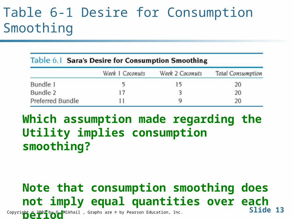
Copyright © 2002 by O. Mikhail , Graphs are © by Pearson Education, Inc. Slide 13
Table 6-1 Desire for Consumption Smoothing
Which assumption made regarding the Utility implies consumption smoothing?
Note that consumption smoothing does not imply equal quantities over each period

Copyright © 2002 by O. Mikhail , Graphs are © by Pearson Education, Inc. Slide 14
Figure 6-3 A Consumer Who Is a Lender
BD: Savings
Endowment

Copyright © 2002 by O. Mikhail , Graphs are © by Pearson Education, Inc. Slide 15
Figure 6-4 A Consumer Who Is a Borrower
Endowment
BD: Borrowing

THE GAME
Changes in:
• Current income
• Future income
• Real interest rate

GAME I an Increase in CURRENT Income

Copyright © 2002 by O. Mikhail , Graphs are © by Pearson Education, Inc. Slide 18
GAME I : An increase in CURRENT income
Intra-Temporal: an increase in income (same as an increase in dividend income or a reduction in taxes) pure income effect c and labor
Inter-Temporal: What will be the effect on c, c’ and s ?

Copyright © 2002 by O. Mikhail , Graphs are © by Pearson Education, Inc. Slide 19
Figure 6-5 The Effects of an Increase in Current Income for a Lender
E1E2
yOld
Endowment
New Endowment
Same Slope r did not change

Copyright © 2002 by O. Mikhail , Graphs are © by Pearson Education, Inc. Slide 20
Figure 6-5 The Effects of an Increase in Current Income for a Lender - Continued
AD is yAF is c
FD is s
Smooth consumption + c, c’ normal goods c, c’ increase

Copyright © 2002 by O. Mikhail , Graphs are © by Pearson Education, Inc. Slide 21
Figure 6-6 Percentage Deviations from Trend in GDP and Consumption, 1982-1999
More variableMore variable
SmootherSmoother

Copyright © 2002 by O. Mikhail , Graphs are © by Pearson Education, Inc. Slide 22
Excess Variability of Consumption
The observed fact that measured consumption is more volatile than theory appears to predict.
Proposed reasons: Capital market imperfections Change in market prices

GAME II an Increase in FUTURE Income

Copyright © 2002 by O. Mikhail , Graphs are © by Pearson Education, Inc. Slide 24
GAME II : An increase in FUTURE income
Intra-Temporal : when it happens, treat it as an increase in current income.
Inter-Temporal : increase present consumption to smooth the consumption pattern, by borrowing.

Copyright © 2002 by O. Mikhail , Graphs are © by Pearson Education, Inc. Slide 25
Figure 6-7 An Increase in Future Income
FD is s
AD is y’
AF is c’
c1c2 is c

GAME III Temporary vs. Permanent
and the Permanent Income hypothesis

Copyright © 2002 by O. Mikhail , Graphs are © by Pearson Education, Inc. Slide 27
Permanent vs. Temporary increase in income
Temporary increase in income Ex: Winning a lottery. Expect to increase current c by small amount.
Permanent increase in income Ex: Promotion, salary raise. Expect to increase current c by a larger amount.

Copyright © 2002 by O. Mikhail , Graphs are © by Pearson Education, Inc. Slide 28
Friedman’s Permanent Income Hypothesis
A primary determinant for current consumption is permanent income, which is closely related to lifetime wealth.
Therefore, changes in temporary income have little influence on current consumption. Changes to permanent income have much larger effect on current consumption.
Do you remember the Keynesian consumption function?

Copyright © 2002 by O. Mikhail , Graphs are © by Pearson Education, Inc. Slide 29
Why Important?
Tax Cut
If consumers perceive the tax cut to be temporary then …..
If consumers perceive the tax cut to be permanent then …..

Copyright © 2002 by O. Mikhail , Graphs are © by Pearson Education, Inc. Slide 30
Model incorporates Temporary vs. Permanent
How?
Temporary: increase in current income.
Permanent: increase in current and future income.

Copyright © 2002 by O. Mikhail , Graphs are © by Pearson Education, Inc. Slide 31
Figure 6-8 Temporary Versus Permanent Increases in Income
Original
HL Temporary increase in y
Permanent case no saving c1c3 = y2 – y1

Copyright © 2002 by O. Mikhail , Graphs are © by Pearson Education, Inc. Slide 32
Figure 6-9 Stock Prices and Nondurable Consumption, 1947-1999
More VolatileMore VolatilePositive Correlation ?Positive Correlation ?

Copyright © 2002 by O. Mikhail , Graphs are © by Pearson Education, Inc. Slide 33
Figure 6-10 Scatter Plot of Percentage Deviations from Trend in Nondurable Consumption Versus Percentage Deviations from Trend in a Stock Price Index
Positive CorrelationPositive Correlation

GAME IV
A change in the Real Interest Rate

Copyright © 2002 by O. Mikhail , Graphs are © by Pearson Education, Inc. Slide 35
NOTATION
Real interest rate r
Nominal interest rate R

Copyright © 2002 by O. Mikhail , Graphs are © by Pearson Education, Inc. Slide 36
Change in the REAL INTEREST RATE
will change the relative price (1/1+r) of leisure and consumption.
r future consumption is cheaper relative to current consumption.
r income and substitution effects r budget steeper [slope = - (1+r)]

Copyright © 2002 by O. Mikhail , Graphs are © by Pearson Education, Inc. Slide 37
Example
Let y = $20 and y’ = $0, no taxes. r = 50%save $10, c = $10 c’= $15
r = 100%save $10, c = $10 c’= $20
The Point: r future consumption is cheaper relative to current consumption.

Copyright © 2002 by O. Mikhail , Graphs are © by Pearson Education, Inc. Slide 38
Figure 6-11 An Increase in the Real Interest Rate
c’ = – (1+r) c + we (1+r)
The budget pivot around the Endowment point
Copyright © 2002 by O. Mikhail , Graphs are © by Pearson Education, Inc. Slide 39
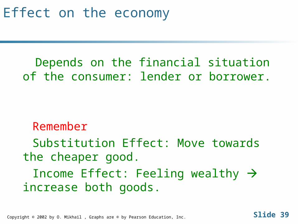
Effect on the economy
Depends on the financial situation of the consumer: lender or borrower.
Remember
Substitution Effect: Move towards the cheaper good.
Income Effect: Feeling wealthy increase both goods.

Copyright © 2002 by O. Mikhail , Graphs are © by Pearson Education, Inc. Slide 40
Figure 6-12 An Increase in the Real Interest Rate for a Lender
AD : Substitution Effect
DB : Income Effect

Copyright © 2002 by O. Mikhail , Graphs are © by Pearson Education, Inc. Slide 41
Figure 6-13 An Increase in the Real Interest Rate for a Borrower
AD : Substitution Effect
DB : Income Effect

Copyright © 2002 by O. Mikhail , Graphs are © by Pearson Education, Inc. Slide 42
Intertemporal Substitution Effect
For both (lender/borrower), a higher real interest rate lowers the relative price of future consumption in terms of current consumption substitution of future consumption for current consumption increase in savings

Copyright © 2002 by O. Mikhail , Graphs are © by Pearson Education, Inc. Slide 43
Table 6-2 and Table 6-3

Copyright © 2002 by O. Mikhail , Graphs are © by Pearson Education, Inc. Slide 44
Figure 6-14 Example with Perfect Complements
Preferences
Extreme consumption smoothing, the consumer desire c and c’ in fixed proportions.

The Point

Copyright © 2002 by O. Mikhail , Graphs are © by Pearson Education, Inc. Slide 46
Figure 6-15 A Consumer’s Demand for Current Consumption Goods, cd, as a Function of Current Income
GAME I
Consumption increases with income
Slope < 1 because of consumption-smoothing motive, some income is always saved.

Copyright © 2002 by O. Mikhail , Graphs are © by Pearson Education, Inc. Slide 47
Figure 6-16 A Shift in a Consumer’s Demand for Current Consumption
Shifters are GAME II and GAME IV
y’ (+) and r (-)

Copyright © 2002 by O. Mikhail , Graphs are © by Pearson Education, Inc. Slide 48
Government
Current Budget: G = T + B
Future Budget: G’ + (1+r) B = T’
Collapse into a single PV budget
G + G’/(1+r) = T + T’/(1+r)
PV(G) = PV(T)

Copyright © 2002 by O. Mikhail , Graphs are © by Pearson Education, Inc. Slide 49
Competitive Equilibrium
Describe the competitive Equilibrium for this ECN.

Copyright © 2002 by O. Mikhail , Graphs are © by Pearson Education, Inc. Slide 50
Ricardian Equivalence Theorem
A change in the timing of taxes by the government is neutral, i.e., has no real effects.
This implies that government deficits do not matter.
By saving/borrowing, the consumer offsets the government action.

Copyright © 2002 by O. Mikhail , Graphs are © by Pearson Education, Inc. Slide 51
The Ricardian Equivalence Theorem
If current (G) and future government spending (G’) are held constant, then a change in current taxes (t) with an equal and opposite change in the present value of future taxes (PV(t’)) leaves the equilibrium real interest rate (r) and the consumptions of individuals unchanged.

Copyright © 2002 by O. Mikhail , Graphs are © by Pearson Education, Inc. Slide 52
Four Assumptions
Taxes change by the same amount for all consumers, in the present and the future.
Any debt issued by the government is paid during the lifetimes of the people alive when the debt was issued.
Taxes are lump sum. Perfect credit markets.

Ricardian Equivalence Numerical Example p. 198

Copyright © 2002 by O. Mikhail , Graphs are © by Pearson Education, Inc. Slide 54
Figure 6-17 Ricardian Equivalence with a Cut in Current Taxes for a Lender
Original
Post tax cut
Same Unchanged

Copyright © 2002 by O. Mikhail , Graphs are © by Pearson Education, Inc. Slide 55
Credit Market Imperfections
Role of credit market imperfections and the Ricardian Equivalence

Copyright © 2002 by O. Mikhail , Graphs are © by Pearson Education, Inc. Slide 56
Figure 6-18 A Consumer Facing Different Lending and Borrowing Rates

Copyright © 2002 by O. Mikhail , Graphs are © by Pearson Education, Inc. Slide 57
Figure 6-19 Effects of a Tax Cut for a Consumer with Different Borrowing and Lending Rates

The Ricardian Equivalence v.s.
President Bush in 1992

Copyright © 2002 by O. Mikhail , Graphs are © by Pearson Education, Inc. Slide 59
Figure 6-20 Deviations from Trend in Consumption, 1947-1999
Is there any evidence?