copernicus global land operations cryosphere and …...mask (white=volcanic soil) obtained after...
TRANSCRIPT
Copernicus Global Land Operations – Lot 2 Date Issued: 18.10.2018 Issue: I1.10
Copernicus Global Land Operations
“Cryosphere and Water” ”CGLOPS-2”
Framework Service Contract N° 199496 (JRC)
ALGORITHM THEORETHICAL BASIS DOCUMENT
WATER BODIES
PROBA-V 300M
VERSION 1
Issue I1.10
Organization name of lead contractor for this deliverable: VITO
Book Captain: I. Reusen (VITO)
Contributing Authors: L. Bertels (VITO)
D. Wolfs (VITO)

Copernicus Global Land Operations – Lot 2 Date Issued: 18.10.2018 Issue: I1.10
Document-No. CGLOPS2_ATBD_WB300m_V1
© C-GLOPS2 consortium
Issue: I1.10 Date: 18.10.2018 Page: 2 of 53
Copernicus Global Land Operations – Lot 2 Date Issued: 18.10.2018 Issue: I1.10
Document-No. CGLOPS2_ATBD_WB300m_V1
© C-GLOPS2 consortium
Issue: I1.10 Date: 18.10.2018 Page: 3 of 53
Dissemination Level PU Public X
PP Restricted to other programme participants (including the Commission Services)
RE Restricted to a group specified by the consortium (including the Commission Services)
CO Confidential, only for members of the consortium (including the Commission Services)

Copernicus Global Land Operations – Lot 2 Date Issued: 18.10.2018 Issue: I1.10
Document-No. CGLOPS2_ATBD_WB300m_V1
© C-GLOPS2 consortium
Issue: I1.10 Date: 18.10.2018 Page: 4 of 53
Document Release Sheet
Copernicus Global Land Operations – Lot 2 Date Issued: 18.10.2018 Issue: I1.10
Document-No. CGLOPS2_ATBD_WB300m_V1
© C-GLOPS2 consortium
Issue: I1.10 Date: 18.10.2018 Page: 5 of 53
Change Record
Issue/Rev Date Page(s) Description of Change Release
06.09.2017 All First issue I1.00
I1.00 01.08.2018 All Revision after review meeting I1.10

Copernicus Global Land Operations – Lot 2 Date Issued: 18.10.2018 Issue: I1.10
Document-No. CGLOPS2_ATBD_WB300m_V1
© C-GLOPS2 consortium
Issue: I1.10 Date: 18.10.2018 Page: 6 of 53
TABLE OF CONTENTS
1 Background of the document ............................................................................................. 12
1.1 Executive Summary ............................................................................................................... 12
1.2 Scope and Objectives............................................................................................................. 12
1.3 Content of the document....................................................................................................... 12
1.4 Related documents ............................................................................................................... 12
1.4.1 Applicable documents ................................................................................................................................ 12
1.4.2 Input ............................................................................................................................................................ 12
1.4.3 Output ......................................................................................................................................................... 13
1.4.4 External Documents .................................................................................................................................... 13
2 Review of Users Requirements ........................................................................................... 14
3 Methodology Description .................................................................................................. 16
3.1 Overview .............................................................................................................................. 16
3.2 The retrieval Algorithm ......................................................................................................... 17
3.2.1 Outline ........................................................................................................................................................ 17
3.2.2 Basic underlying assumptions ..................................................................................................................... 19
3.2.3 Related and previous applications .............................................................................................................. 19
3.2.4 Alternative methodologies currently in use ............................................................................................... 21
3.2.5 Input data.................................................................................................................................................... 21
3.2.6 Output product ........................................................................................................................................... 25
3.2.7 Methodology............................................................................................................................................... 26
3.2.8 Limitations .................................................................................................................................................. 51
3.3 Quality Assessment ............................................................................................................... 52
3.4 Risk of failure and Mitigation measures ................................................................................. 52
4 References ........................................................................................................................ 53
Copernicus Global Land Operations – Lot 2 Date Issued: 18.10.2018 Issue: I1.10
Document-No. CGLOPS2_ATBD_WB300m_V1
© C-GLOPS2 consortium
Issue: I1.10 Date: 18.10.2018 Page: 7 of 53
List of Figures
Figure 1: General overview of the Water Bodies Detection Algorithm. .......................................... 16
Figure 2: Outline of the Water Bodies Detection Algorithm. ........................................................... 18
Figure 3: Location in Northern South-Sudan (10°0’N, 31°80’E). a) False water bodies were
detected because of dark soils. b) By applying the extra check on the MWEM most of the
commission errors could be prevented. .................................................................................. 20
Figure 4: Location in Southern Spain (38°40N, 7°4’W). a) Due to the strict Water Bodies Potential
Mask parts of the lake were not detected as water. b) The MWEM overrules the WBPM and as
such reduces the omission errors. ......................................................................................... 21
Figure 5: a) This Google Earth image shows an area over the Alps (Upper left corner: 48°08’25” N,
5°40’0” E). b) The permanent glacier mask for the same area in (a). ..................................... 23
Figure 6: a) Google Earth image showing part of northern Ethiopia and southern Eritrea with the
dark volcanic soils manually delineated (red polygons). b) Dekad MC10_20140521 for the
same area with the derived dark volcanic soils shape file overlaid. c) The final volcanic soil
mask (white=volcanic soil) obtained after rasterizing the shape file. ....................................... 24
Figure 7: a) The high resolution Maximum Water Extent product of JRC’s Global Surface Water
dataset shows where in the last 32 years water was ever detected (blue colored). b) The
PROBA-V 300 m resolution Maximum Water Extent Mask is derived from the Maximum Water
Extent product of JRC’s Global Surface Water dataset. Both images have the PROBA-V 300
m raster overlaid (red). The shown water reservoir is located in India (25°25’N, 77°55’E). ..... 25
Figure 8: MC10 algorithm flow. ..................................................................................................... 28
Figure 9: Decision tree for MC10 observation type classification. .................................................. 29
Figure 10: a) Part of the 90 m spatial resolution GLSDEM over Rift Valley in Ethiopia. b) The
detected lowest points for this area are colored yellow. The larger sized colored areas are
areas of equally low elevation which correspond to some smaller lakes in the region. ........... 31
Figure 11: Expanding the initially detected lowest point by systematically rising an imaginary water
level in steps of 1 m. The corresponding 90 m spatial resolution pixels are indicated by the
dots at the bottom. ................................................................................................................. 32
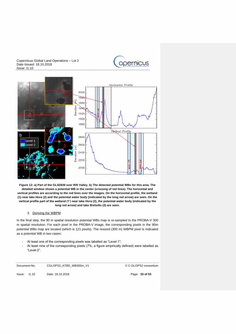
Figure 12: a) Part of the GLSDEM over Rift Valley. b) The detected potential WBs for this area.
The detailed window shows a potential WB in the center (crossing of red lines). The horizontal
and vertical profiles are according to the red lines over the images. On the horizontal profile,
the wetland (1) near lake Hora (2) and the potential water body (indicated by the long red
arrow) are seen. On the vertical profile part of the wetland (1’) near lake Hora (2), the potential
water body (indicated by the long red arrow) and lake Bishoftu (3) are seen. ......................... 33
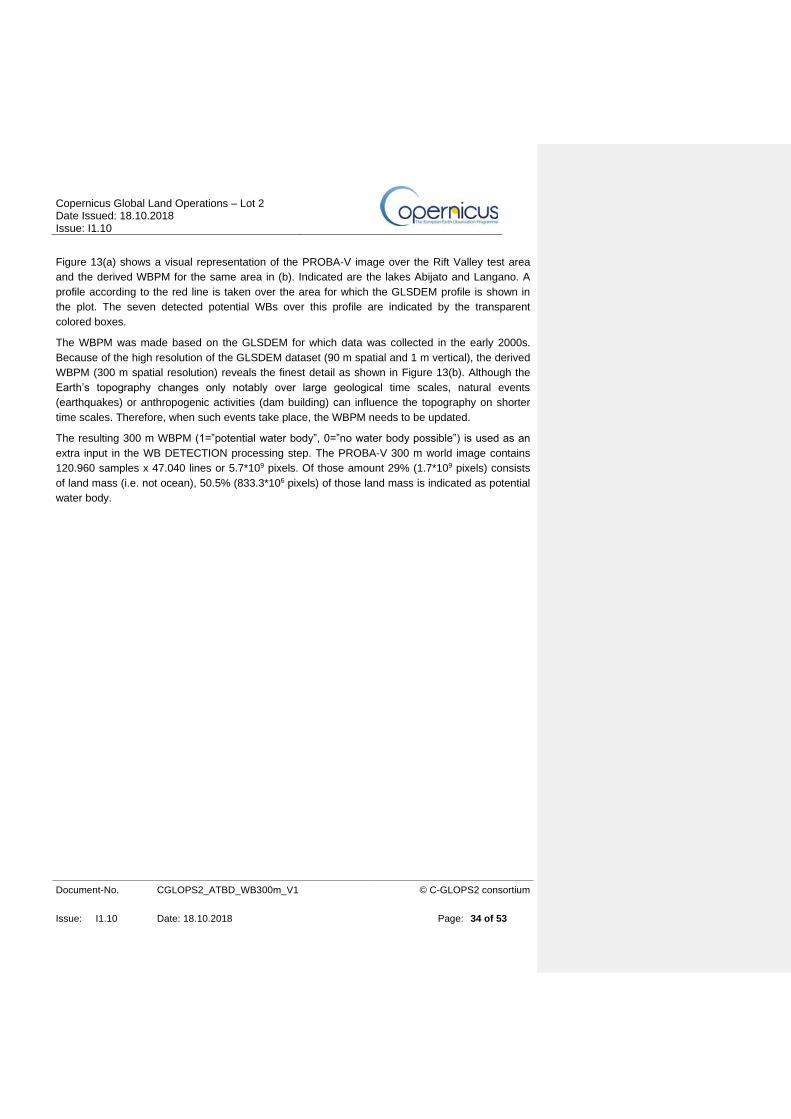
Figure 13: a) Part of image MC10_20131021 taken over the Rift Valley in Ethiopia (SWIR, NIR and
Red bands assigned to the RGB channels resp.). b) The WBPM for the same area in (a)
Copernicus Global Land Operations – Lot 2 Date Issued: 18.10.2018 Issue: I1.10
Document-No. CGLOPS2_ATBD_WB300m_V1
© C-GLOPS2 consortium
Issue: I1.10 Date: 18.10.2018 Page: 8 of 53
(white=potential water body, black=no water body possible). The plot shows the vertical
GLSDEM profile according to the red line. Marked with the blue boxes are the seven potential
WBs. The arrows indicate the location of lake Abijato (1) and lake Langano (2). ................... 35
Figure 14: The HSV color space. .................................................................................................. 36
Figure 15: The first part of the WBDA comprises invalid data filtering. .......................................... 37
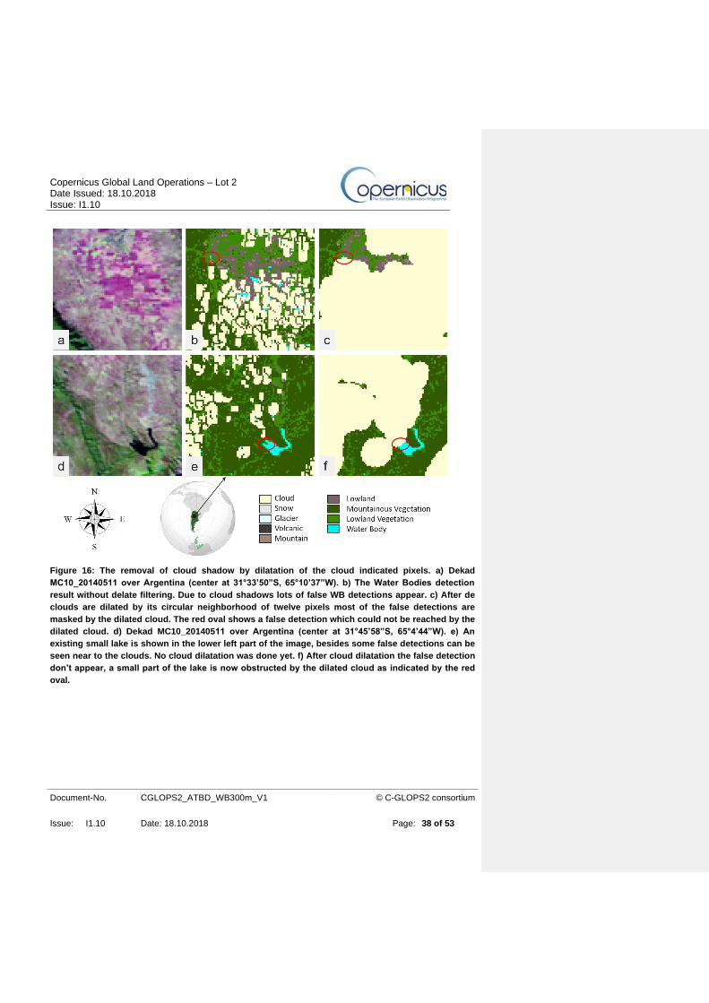
Figure 16: The removal of cloud shadow by dilatation of the cloud indicated pixels. a) Dekad
MC10_20140511 over Argentina (center at 31°33’50”S, 65°10’37”W). b) The Water Bodies
detection result without delate filtering. Due to cloud shadows lots of false WB detections
appear. c) After de clouds are dilated by its circular neighborhood of twelve pixels most of the
false detections are masked by the dilated cloud. The red oval shows a false detection which
could not be reached by the dilated cloud. d) Dekad MC10_20140511 over Argentina (center
at 31°45’58”S, 65°4’44”W). e) An existing small lake is shown in the lower left part of the
image, besides some false detections can be seen near to the clouds. No cloud dilatation was
done yet. f) After cloud dilatation the false detection don’t appear, a small part of the lake is
now obstructed by the dilated cloud as indicated by the red oval. .......................................... 38
Figure 17: The second part of the WBDA comprises Incompatibility Masking. .............................. 39
Figure 18: The last part of the WBDA comprises actual Water Body Detection based on threshold
levels on the HUE and VALUE bands. The thresholds consist of two parabolic functions. ..... 40
Figure 19: 2D scatter plot of the Vietnam test area showing the final threshold levels. Land pixels
are indicated by the dark grey dots, reference WBs (obtained from Landsat 8) are indicated by
the colored plus symbols for different ranges of water surface ratios. A further refinement of
the thresholds is not possible because WB pixels and land pixels are intermixed. ................. 43
Figure 20: Location of the Landsat scenes used to define the detection method. .......................... 44
Figure 21: Workflow for the extraction of reference water bodies using Landsat-8 scenes. An as
much as possible cloud free scene is searched for the required geographical location and time
period. After pre-processing and HSV color transform of the Landsat-8 scene, WB detection
was done using a Decision Tree Classifier (DTC). The obtained Landsat-8 WBs are
subsequently used to calculate the Water Surface Ratio using the spatial information from the
PROBA-V image. ................................................................................................................... 45
Figure 22: Decision Tree Classifier for WB detection on Landsat-8 images. A check on different
bands and on cloud cover removes incompatible pixels from the scene. A check on HUE and
VALUE is used to detect water bodies. .................................................................................. 46
Figure 23: 2D scatter plot of the WB frequency (WBf) and the number of continuous temporal WB
observations (mctWBs) for the Rift Valley test area calculated for the 31 available dekads. The
Water Body Occurrence levels are indicated by the different colored areas. .......................... 51

Copernicus Global Land Operations – Lot 2 Date Issued: 18.10.2018 Issue: I1.10
Document-No. CGLOPS2_ATBD_WB300m_V1
© C-GLOPS2 consortium
Issue: I1.10 Date: 18.10.2018 Page: 9 of 53
List of Tables
Table 1: GCOS requirements for areas of water bodies as Lakes and Land cover Essential Climate
Variables (GCOS-200, 2016) ................................................................................................. 15
Table 2: Thresholds for water body detection are applied on the HUE and VALUE, which are
obtained after HSV color transformation of the SWIR, NIR and Red bands, on the NDVI and
on the VALUE as an additional check besides the NDVI threshold check (NV). ..................... 19
Table 3: Spectral characteristics of the PROBA-V bands .............................................................. 22
Table 4: Status Map bit mapping of the PROBA-V data ................................................................ 22
Table 5: Output product legend. .................................................................................................... 26
Table 6: Output QUAL product legend. The colored entries are the occurrence values. ............... 26
Table 7: Status Map (SM) bit mapping. ......................................................................................... 30
Table 8: Landsat-8 scenes used to define the PROBA-V water bodies detection thresholds. ....... 44
Table 9: The results for eight different settings of the threshold levels. The overall accuracy (OA),
omission errors (OE) and the commission errors (CE) are listed in percentage. The OEs are
given for six ranges of minimum WSR . The figures are calculated over the 22 test regions for
the period Oct2013 – May2014. The green indicated entries show the best results and are the
final threshold levels. ............................................................................................................. 48
Table 10: Omission and commission errors are caused by several reasons. ................................ 52

Copernicus Global Land Operations – Lot 2 Date Issued: 18.10.2018 Issue: I1.10
Document-No. CGLOPS2_ATBD_WB300m_V1
© C-GLOPS2 consortium
Issue: I1.10 Date: 18.10.2018 Page: 10 of 53
List of Acronyms
ACCAm Automatic Cloud Cover Assessment - modified
ATBD Algorithm Theoretical Basis Document
DEM Digital Elevation Model
DTC Decision Tree Classifier
ECV Essential Climate Variables
ESA European Space Agency
GCOS Global Climate Observing System
GIO GMES Initial Operations
GL Global Land
GLIMS Global Land Ice Measurements from Space
GLSDEM Global Land Survey Digital Elevation Model
GMES Global Monitoring for Environment and Security
GSW Global Surface Water
GWW Global Water Watch
HSV Hue, Saturation and Value colour system
IFOV Instantaneous Field Of View
LC Land Cover
MC Mean Compositing
MC10 10-day mean compositing synthesis
NDVI Normalized Difference Vegetation Index
MWE-GSW Maximum Water Extent product of JRC’s Global Surface Water
MWEM Maximum Water Extent Mask
NIR Near Infrared
NMOD Number of valid Observations used in 10-daily compositing period
NOBS Number of satellite overpasses within the 10-daily compositing period
NSIDC National Snow and Ice Data Centre
PGM Permanent Glaciers Mask
PROBA-V Vegetation instrument on board of PROBA satellite
QUAL Quality Layer
RGB Red, Green and Blue colour system
S1-TOC The PROBA-V daily Top-Of-Canopy synthesis products
SM Status Map
SMAC Simplified Model for Atmospheric Correction
SPOT Satellite Pour l’Observation de la Terre
SRTM Shuttle Radar Topography Mission
SVP Service Validation Plan
SWIR Short Wavelength Infrared
SZA Solar Zenith Angle
TOA Top of Atmosphere
TOC Top of Canopy
Copernicus Global Land Operations – Lot 2 Date Issued: 18.10.2018 Issue: I1.10
Document-No. CGLOPS2_ATBD_WB300m_V1
© C-GLOPS2 consortium
Issue: I1.10 Date: 18.10.2018 Page: 11 of 53
UNFCCC United Nations Framework Convention on Climate Change
USGS United States Geological Survey
VITO Vlaamse Instelling voor Technologisch Onderzoek (Flemish Institute for Technological Research), Belgium
VSM Volcanic Soils Mask
WB Water Body
WBDA Water Bodies Detection Algorithm
WBO Water Bodies Occurrence
WBPM Water Bodies Potential Mask
WBPV PROBA-V Water Bodies product
WSR Water Surface Ratio
2D Two dimensional
Copernicus Global Land Operations – Lot 2 Date Issued: 18.10.2018 Issue: I1.10
Document-No. CGLOPS2_ATBD_WB300m_V1
© C-GLOPS2 consortium
Issue: I1.10 Date: 18.10.2018 Page: 12 of 53
1 BACKGROUND OF THE DOCUMENT
1.1 EXECUTIVE SUMMARY
The Copernicus Land Service continuously monitors the status of land territories to generate geo-
information at both local and global scale. Its Global Land component provides several bio-
geophysical products describing the status of the land surface on a global scale and its evolution.
Production and delivery of the parameters are to take place in a timely manner and are
complemented by the constitution of long time series.
This Algorithm Theoretical Basis Document (ATBD) describes the method for detecting Water
Bodies (WB) using PROBA-V at 333m resolution on a global scale. The method for deriving the
thresholds and the evaluation of the performance of the algorithm are based on the approach
developed by Pekel et al., 2014 and on the methods developed for the PROBA-V 1 km product as
described in GIOGL1_ATBD_WB1km-PROBAV-V2.
1.2 SCOPE AND OBJECTIVES
The scope of this document is to describe the theoretical basis and justification that underpins the
implementation of the Copernicus Global Land Water Bodies product . It details the methodology
applied on the PROBA-V 333m data. Moreover, it provides an evaluation of the algorithm
performance and a description of the limitations.
1.3 CONTENT OF THE DOCUMENT
This ATBD is structured as follows:
• Chapter 1 (this chapter) introduces the product
• Chapter 2 reviews the user requirements
• Chapter 3 describes the methodology used to generate the Water Bodies product
• Chapter 4 lists the references used in this document
1.4 RELATED DOCUMENTS
1.4.1 Applicable documents
AD1: Annex I – Technical Specifications JRC/IPR/2015/H.5/0026/OC to Contract Notice 2015/S
151-277962 of 7th August 2015
AD2: Appendix 1 – Copernicus Global land Component Product and Service Detailed Technical
requirements to Technical Annex to Contract Notice 2015/S 151-277962 of 7th August 2015
1.4.2 Input
Document ID Descriptor
Copernicus Global Land Operations – Lot 2 Date Issued: 18.10.2018 Issue: I1.10
Document-No. CGLOPS2_ATBD_WB300m_V1
© C-GLOPS2 consortium
Issue: I1.10 Date: 18.10.2018 Page: 13 of 53
CGLOPS2_SSD Service Specifications of the Global Component of
the Copernicus Land Service.
1.4.3 Output
Document ID Descriptor
CGLOPS2_PUM_WB300m_V1 Product User Manual for version 1 of the 300 m
Water Bodies product from PROBA-V.
CGLOPS2_QAR_WB300m_V1 Validation Report describing the results of the
scientific quality assessment for version 1 of the 300
m Water Bodies product from PROBA-V.
1.4.4 External Documents
Document ID Descriptor
PROBA-V http://proba-v.vgt.vito.be/
PROBA-V PUM
Products User Manual of PROBA-V data, available on
http://proba-v.vgt.vito.be/sites/proba-v.vgt.vito.be/files/probav-
products_user_manual_v2.2_0.pdf
Commenté [BL1]: RID 1408: document updated
Copernicus Global Land Operations – Lot 2 Date Issued: 18.10.2018 Issue: I1.10
Document-No. CGLOPS2_ATBD_WB300m_V1
© C-GLOPS2 consortium
Issue: I1.10 Date: 18.10.2018 Page: 14 of 53
2 REVIEW OF USERS REQUIREMENTS
According to the applicable document [AD2], the user’s requirements relevant for Water Bodies
PROBA-V 300 m are:
• Definition: permanent and seasonal water bodies, natural and man-made, independently
of their size. Include but are not restricted to the lakes of the Global terrestrial Network for
lakes.
• Geometric properties:
o Location accuracy shall be 1/3rd of the at-nadir instantaneous field of view.
o Pixel co-ordinates shall be given for center of pixel
• Geographical coverage:
o Geographic projection: regular latitude/longitude
o Geodetical datum: WGS84
o Coordinate position: center pixel
o Pixel size: 1/336° - accuracy: min 10 digits
o Global window coordinates:
▪ upper left: 180°W - 75°N
▪ bottom right: 180°E - 56°S
• Ancillary information:
o the per-pixel date of the individual measurements or the start-end dates of the
period actually covered
o quality indicators, with explicit per-pixel identification of the cause of anomalous
parameter result
• Accuracy requirements:
o Baseline: wherever applicable the bio-geophysical parameters should meet the
internationally agreed accuracy standards laid down in the document “Systematic
Observation Requirements for Satellite-Based Products for Climate”. Additional
details to the satellite based component of the Implementation Plan for the Global
Observing System for Climate in Support of the UNFCCC are available in the
document WMO (GCOS-#200, 2016) (see Table 1).
o Target: considering data usage by that part of the user community focused on
operational monitoring at (sub-) national scale, accuracy standards may apply not
on averages at global scale, but at a finer geographic resolution and in any event at
least at biome level.
Commenté [BL2]: RID 1383

Copernicus Global Land Operations – Lot 2 Date Issued: 18.10.2018 Issue: I1.10
Document-No. CGLOPS2_ATBD_WB300m_V1
© C-GLOPS2 consortium
Issue: I1.10 Date: 18.10.2018 Page: 15 of 53
Regarding this latter accuracy requirement, the water surface biophysical variable
corresponds to different Essential Climate Variables (ECV), i.e. the “land cover” and the
“lakes”.
Table 1: GCOS requirements for areas of water bodies as Lakes and Land cover Essential Climate
Variables (GCOS-200, 2016)
Variable Horizontal
resolution
Temporal
resolution
Accuracy Stability
Areas of
lakes
Equivalent
to 250m
Monthly 5% (maximum error of
omission and commission
in lake area maps);
location accuracy better
than 1/3 of instantaneous
field-of-view (IFOV) with
250m target IFOV
5% (maximum error of
omission and
commission in lake area
maps); location accuracy
better than 1/3 of
instantaneous IFOV with
250m target IFOV
Maps of
land-cover
type
250m 1 year 15% (maximum error of
omission and commission
in mapping individual
classes); location accuracy
better than 1/3 of
instantaneous field-of-view
(IFOV) with 250m target
IFOV
15% (maximum error of
omission and
commission in mapping
individual classes);
location accuracy better
than 1/3 of instantaneous
field-of-view (IFOV) with
250m target IFOV
Copernicus Global Land Operations – Lot 2 Date Issued: 18.10.2018 Issue: I1.10
Document-No. CGLOPS2_ATBD_WB300m_V1
© C-GLOPS2 consortium
Issue: I1.10 Date: 18.10.2018 Page: 16 of 53
3 METHODOLOGY DESCRIPTION
3.1 OVERVIEW
The Global Land Water Bodies 300 m Version 1 product is a 10-daily synthesis product derived
from Top of Canopy (TOC) PROBA-V 333 m data. The product consists of 2 layers, the basic
Water Bodies (WB) layer which tells which pixels contain water and which not, and the Quality
Layer (QUAL) which tells something about the water body’s occurrences and as such can be used
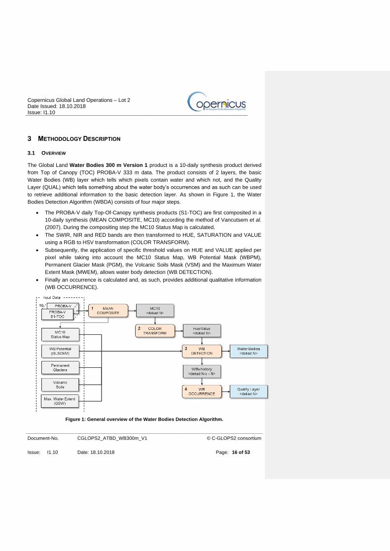
to retrieve additional information to the basic detection layer. As shown in Figure 1, the Water
Bodies Detection Algorithm (WBDA) consists of four major steps.
• The PROBA-V daily Top-Of-Canopy synthesis products (S1-TOC) are first composited in a
10-daily synthesis (MEAN COMPOSITE, MC10) according the method of Vancutsem et al.
(2007). During the compositing step the MC10 Status Map is calculated.
• The SWIR, NIR and RED bands are then transformed to HUE, SATURATION and VALUE
using a RGB to HSV transformation (COLOR TRANSFORM).
• Subsequently, the application of specific threshold values on HUE and VALUE applied per
pixel while taking into account the MC10 Status Map, WB Potential Mask (WBPM),
Permanent Glacier Mask (PGM), the Volcanic Soils Mask (VSM) and the Maximum Water
Extent Mask (MWEM), allows water body detection (WB DETECTION).
• Finally an occurrence is calculated and, as such, provides additional qualitative information
(WB OCCURRENCE).
Figure 1: General overview of the Water Bodies Detection Algorithm.
Copernicus Global Land Operations – Lot 2 Date Issued: 18.10.2018 Issue: I1.10
Document-No. CGLOPS2_ATBD_WB300m_V1
© C-GLOPS2 consortium
Issue: I1.10 Date: 18.10.2018 Page: 17 of 53
3.2 THE RETRIEVAL ALGORITHM
3.2.1 Outline
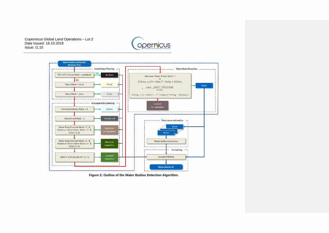
A schematic overview of the Water Body Detection Algorithm (WBDA) is shown by the decision
tree in Figure 2.
Developing the WBDA involved three main steps which are described in the following paragraphs:
• Invalid data filtering
• Incompatibility masking
• Water body detection
Although WB detection is based on thresholds on the HUE and VALUE, the description of the
different steps of the Decision Tree is given in their actual sequence.
Copernicus Global Land Operations – Lot 2 Date Issued: 18.10.2018 Issue: I1.10
Figure 2: Outline of the Water Bodies Detection Algorithm.
Copernicus Global Land Operations – Lot 2 Date Issued: 18.10.2018 Issue: I1.10
3.2.2 Basic underlying assumptions
Water bodies have specific spectral features that mostly distinguish them from the other Earth
surface objects. The red, NIR and SWIR bands are HSV-color transformed. After that a threshold
on the HUE and VALUE bands are applied for the detection of water bodies. To avoid confusion
with other objects on the Earth’s surface which have identical spectral properties as water bodies,
additional data layers are used: the permanent glacier mask, volcanic soil mask, water body
potential mask and maximum water extent mask are used to reduce commission errors.
3.2.3 Related and previous applications
The water bodies detection algorithm for the PROBA-V 300 m collection is related to the water
bodies detection algorithm developed for the PROBA-V 1 km and SPOT/VGT collection. Two
additional changes have been implemented.
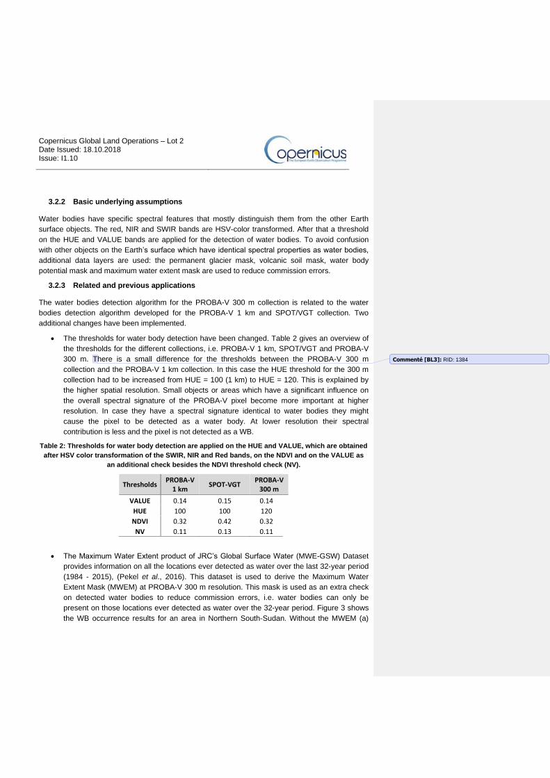
• The thresholds for water body detection have been changed. Table 2 gives an overview of
the thresholds for the different collections, i.e. PROBA-V 1 km, SPOT/VGT and PROBA-V
300 m. There is a small difference for the thresholds between the PROBA-V 300 m
collection and the PROBA-V 1 km collection. In this case the HUE threshold for the 300 m
collection had to be increased from HUE = 100 (1 km) to HUE = 120. This is explained by
the higher spatial resolution. Small objects or areas which have a significant influence on
the overall spectral signature of the PROBA-V pixel become more important at higher
resolution. In case they have a spectral signature identical to water bodies they might
cause the pixel to be detected as a water body. At lower resolution their spectral
contribution is less and the pixel is not detected as a WB.
Table 2: Thresholds for water body detection are applied on the HUE and VALUE, which are obtained
after HSV color transformation of the SWIR, NIR and Red bands, on the NDVI and on the VALUE as
an additional check besides the NDVI threshold check (NV).
Thresholds PROBA-V
1 km SPOT-VGT
PROBA-V 300 m
VALUE 0.14 0.15 0.14
HUE 100 100 120
NDVI 0.32 0.42 0.32
NV 0.11 0.13 0.11
• The Maximum Water Extent product of JRC’s Global Surface Water (MWE-GSW) Dataset
provides information on all the locations ever detected as water over the last 32-year period
(1984 - 2015), (Pekel et al., 2016). This dataset is used to derive the Maximum Water
Extent Mask (MWEM) at PROBA-V 300 m resolution. This mask is used as an extra check
on detected water bodies to reduce commission errors, i.e. water bodies can only be
present on those locations ever detected as water over the 32-year period. Figure 3 shows
the WB occurrence results for an area in Northern South-Sudan. Without the MWEM (a)
Commenté [BL3]: RID: 1384

Copernicus Global Land Operations – Lot 2 Date Issued: 18.10.2018 Issue: I1.10
Document-No. CGLOPS2_ATBD_WB300m_V1
© C-GLOPS2 consortium
Issue: I1.10 Date: 18.10.2018 Page: 20 of 53
false detections occur due to dark soils. With the MWEM (b) the false detections don’t
occur and commission errors will be drastically reduced. To reduce omission errors, the
mask overrules the Water Bodies Potential Mask (WBPM). The WBPM, which was derived
from the Global Land Survey Digital Elevation Model (GLSDEM) (USGS, 2008), indicates
on which locations water bodies might be present. Because the GLSDEM was a snapshot
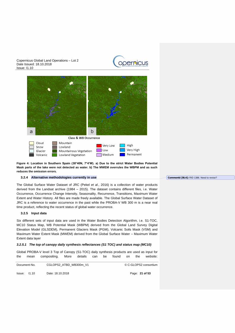
in time it might be too strict in some cases. Figure 4 shows the WB occurrence results for
an area in Spain. Without the MWEM (a) the water reservoir is poorly detected. With the
MWEM (b) the water reservoir is detected in its full size and omission errors will be
drastically reduced.
Figure 3: Location in Northern South-Sudan (10°0’N, 31°80’E). a) False water bodies were detected
because of dark soils. b) By applying the extra check on the MWEM most of the commission errors
could be prevented.
Copernicus Global Land Operations – Lot 2 Date Issued: 18.10.2018 Issue: I1.10
Document-No. CGLOPS2_ATBD_WB300m_V1
© C-GLOPS2 consortium
Issue: I1.10 Date: 18.10.2018 Page: 21 of 53
Figure 4: Location in Southern Spain (38°40N, 7°4’W). a) Due to the strict Water Bodies Potential
Mask parts of the lake were not detected as water. b) The MWEM overrules the WBPM and as such
reduces the omission errors.
3.2.4 Alternative methodologies currently in use
The Global Surface Water Dataset of JRC (Pekel et al., 2016) is a collection of water products
derived from the Landsat archive (1984 – 2015). The dataset contains different files, i.e. Water
Occurrence, Occurrence Change Intensity, Seasonality, Recurrence, Transitions, Maximum Water
Extent and Water History. All files are made freely available. The Global Surface Water Dataset of
JRC is a reference to water occurrence in the past while the PROBA-V WB 300 m is a near real
time product, reflecting the recent status of global water occurrence.
3.2.5 Input data
Six different sets of input data are used in the Water Bodies Detection Algorithm, i.e. S1-TOC,
MC10 Status Map, WB Potential Mask (WBPM) derived from the Global Land Survey Digital
Elevation Model (GLSDEM), Permanent Glaciers Mask (PGM), Volcanic Soils Mask (VSM) and
Maximum Water Extent Mask (MWEM) derived from the Global Surface Water – Maximum Water
Extent data layer
3.2.5.1 The top of canopy daily synthesis reflectances (S1 TOC) and status map (MC10)
Global PROBA-V level 3 Top of Canopy (S1-TOC) daily synthesis products are used as input for
the mean compositing. More details can be found on the website:
Commenté [BL4]: RID 1386. Need to revise?

Copernicus Global Land Operations – Lot 2 Date Issued: 18.10.2018 Issue: I1.10
Document-No. CGLOPS2_ATBD_WB300m_V1
© C-GLOPS2 consortium
Issue: I1.10 Date: 18.10.2018 Page: 22 of 53
https://earth.esa.int/web/guest/data-access/browse-data-products/-/article/proba-v-1km-synthesis-
products-s1-toa-s1-toc-and-s10-toc.
The PROBA-V S1-TOC synthesis product ensures a daily coverage between Lat. 35° N and 75° N,
and between 35° S and 56° S, and a full coverage every two days around the equator (between
35°S and 35°N). The S1 Level 3 Top of Canopy (atmospheric corrections applied) daily synthesis
product is provided at 333 m spatial resolution. Surface reflectance is available for four spectral
bands corresponding to the selected measurement (Table 3). The atmospheric correction is
performed using SMAC 4.0 (Rahman and Dedieu, 1994). Standard input data layers includes
Normalized Difference Vegetation Index (NDVI), geometric viewing and illumination conditions,
reference to date and time of observations four reflectance bands (Table 3) and a status map
containing identification of snow, ice, shadow, clouds, land/sea for every pixel (Table 4). The data
is stored in a szip compressed hdf5 file.
Table 3: Spectral characteristics of the PROBA-V bands
Spectral band Wavelength
BLUE 0.447 – 0.493 µm
RED 0.610 – 0.690 µm
NIR 0.770 – 0.893 µm
SWIR 1.570 – 1.650 µm
Table 4: Status Map bit mapping of the PROBA-V data
Bit Name Description
1 -3 Observation
000: clear
010: undefined
011: cloud
100: snow/ice
4 Land/sea mask 0: sea
1: land
5 SWIR quality flag 0: invalid data
1: valid data
6 NIR quality flag 0: invalid data
1: valid data
7 RED quality flag 0: invalid data
1: valid data
8 (Most significant) BLUE quality flag 0: invalid data
1: valid data
Besides the mean compositing of the reflectance bands, a status map is constructed. It is used as
an extra check in the WB detection algorithm to filter out invalid pixels.

Copernicus Global Land Operations – Lot 2 Date Issued: 18.10.2018 Issue: I1.10
Document-No. CGLOPS2_ATBD_WB300m_V1
© C-GLOPS2 consortium
Issue: I1.10 Date: 18.10.2018 Page: 23 of 53
3.2.5.2 The Water Bodies Potential Mask (WBPM)
Pixels in hilly terrain having low reflectance values due to shadow or dark vegetation are often
confused with WBs. To minimize these commission errors, a Water Bodies Potential Mask
(WBPM) is derived from the Global Land Survey Digital Elevation Model (GLSDEM) (USGS, 2008).
3.2.5.3 The Permanent Glaciers Mask (PGM)
To avoid commission errors due to confusion with permanent glaciers, which often have similar
spectral properties than WBs, a Permanent Glacier Mask (PGM) was constructed. The most recent
permanent glacier data was downloaded from the National Snow and Ice Data Centre (NSIDC,
December 2016) as a shape file which was subsequently rasterized to the PROBA-V image world
size in order to obtain the Permanent Glacier Mask (PGM). When a pixel is indicated as permanent
glacier, it cannot be a water body. Figure 5(a) shows a Google Earth image over the Alps, the
corresponding PGM is shown in (b).
Because the extent of glaciers worldwide are strongly influenced by climate (global warming), the
PGM needs to be frequently updated. An update of the permanent glacier data becomes frequently
available at the NSIDC.
Figure 5: a) This Google Earth image shows an area over the Alps (Upper left corner: 48°08’25” N,
5°40’0” E). b) The permanent glacier mask for the same area in (a).
3.2.5.4 The Volcanic Soils Mask (VSM)
Locations comprised of dark volcanic soils which are spread over wider flat areas are easily
confused with water bodies. To account for these potential commission errors, a Volcanic Soil
Mask (VSM) was made. The geographical locations obtained from the Holocene Volcano List, set-
up by the Global Volcanism Program of the Smithsonian Institution, National Museum of Natural
History (http://www.volcano.si.edu/), were used to locate volcanoes and their dark volcanic soils.
Volcanic soils can be easily located on Google Earth using the information from the Holocene
Volcano List. As shown in Figure 6(a), these areas were manually delineated on the Google Earth
Commenté [BL5]: RID 1387

Copernicus Global Land Operations – Lot 2 Date Issued: 18.10.2018 Issue: I1.10
Document-No. CGLOPS2_ATBD_WB300m_V1
© C-GLOPS2 consortium
Issue: I1.10 Date: 18.10.2018 Page: 24 of 53
image (February 2015). The polygons were exported to shape files as shown in (b) and
subsequently rasterized to a VSM (c). Small errors made during delineation disappear when
rasterizing to the lower resolution PROBA-V pixel size. The geological situation in the volcanic
areas of southern America, i.e. Chili and Peru, is very complex and delineating the volcanic soils in
these areas was not always easy. It is therefore very well possible that some smaller regions in this
area are still missing in the VSM. On the other hand future eruptions might produce new dark
volcanic soils leading to false detected WBs. In both cases an update of the VSM is needed.
Figure 6: a) Google Earth image showing part of northern Ethiopia and southern Eritrea with the dark
volcanic soils manually delineated (red polygons). b) Dekad MC10_20140521 for the same area with
the derived dark volcanic soils shape file overlaid. c) The final volcanic soil mask (white=volcanic
soil) obtained after rasterizing the shape file.
3.2.5.5 The Maximum Water Extent Mask (MWEM)
The Maximum Water Extent product of JRC’s Global Surface Water (MWE-GSW) dataset is used
to create the Maximum Water Extent Mask (MWEM). This dataset provides information on all the
Commenté [BL6]: RID: 1387

Copernicus Global Land Operations – Lot 2 Date Issued: 18.10.2018 Issue: I1.10
Document-No. CGLOPS2_ATBD_WB300m_V1
© C-GLOPS2 consortium
Issue: I1.10 Date: 18.10.2018 Page: 25 of 53
locations ever detected as water over the last 32-year period. The GSW dataset has a spatial
resolution of 1/4000° and therefore needs to be resampled to the PROBA-V 300 m, 1/336° spatial
resolution. For each PROBA-V 300 m pixel, the corresponding pixels in the MWE_GSM are
searched for. A pixel is set in the MWEM if at least one of the corresponding pixels was found to
have ever contained water in the MWE-GSM product (Figure 7a, b).
Figure 7: a) The high resolution Maximum Water Extent product of JRC’s Global Surface Water
dataset shows where in the last 32 years water was ever detected (blue colored). b) The PROBA-V
300 m resolution Maximum Water Extent Mask is derived from the Maximum Water Extent product of
JRC’s Global Surface Water dataset. Both images have the PROBA-V 300 m raster overlaid (red). The
shown water reservoir is located in India (25°25’N, 77°55’E).
3.2.6 Output product
The water bodies product consists of two layers:
• The Water Bodies (WB)
The values of the digital numbers in the first band (WB) are summarized in Table 5. The
values are kept consistent with the version 1, 1 km product over Africa.
Copernicus Global Land Operations – Lot 2 Date Issued: 18.10.2018 Issue: I1.10
Document-No. CGLOPS2_ATBD_WB300m_V1
© C-GLOPS2 consortium
Issue: I1.10 Date: 18.10.2018 Page: 26 of 53
Table 5: Output product legend.
Value Label
0 Sea
70 Water
251 No data
255 No water
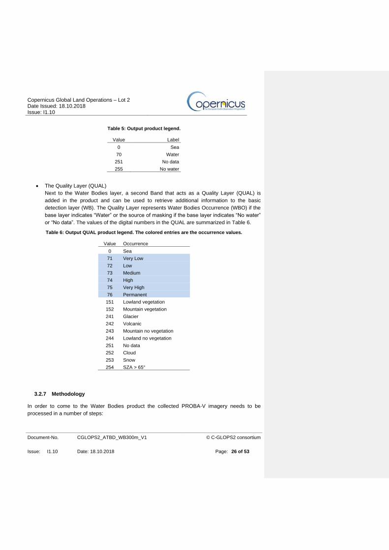
• The Quality Layer (QUAL)
Next to the Water Bodies layer, a second Band that acts as a Quality Layer (QUAL) is
added in the product and can be used to retrieve additional information to the basic
detection layer (WB). The Quality Layer represents Water Bodies Occurrence (WBO) if the
base layer indicates “Water” or the source of masking if the base layer indicates “No water”
or “No data”. The values of the digital numbers in the QUAL are summarized in Table 6.
Table 6: Output QUAL product legend. The colored entries are the occurrence values.
Value Occurrence
0 Sea
71 Very Low
72 Low
73 Medium
74 High
75 Very High
76 Permanent
151 Lowland vegetation
152 Mountain vegetation
241 Glacier
242 Volcanic
243 Mountain no vegetation
244 Lowland no vegetation
251 No data
252 Cloud
253 Snow
254 SZA > 65°
3.2.7 Methodology
In order to come to the Water Bodies product the collected PROBA-V imagery needs to be
processed in a number of steps:
Copernicus Global Land Operations – Lot 2 Date Issued: 18.10.2018 Issue: I1.10
Document-No. CGLOPS2_ATBD_WB300m_V1
© C-GLOPS2 consortium
Issue: I1.10 Date: 18.10.2018 Page: 27 of 53
3.2.7.1 Mean compositing
The MC10 composites (SWIR, NIR, RED, BLUE) are obtained using the mean compositing (MC)
method (Vancutsem et al., 2007) applied on the PROBA-V S1 daily reflectance values over a 10-
days window. The mean compositing algorithm improves the radiometric quality of the temporal
synthesis by averaging the reflectances and therefore reduces the random component of the
noise. Figure 8 depicts the processing flow of the MC10 algorithm.
The mean composite is calculated, pixel by pixel, across the four spectral bands simultaneously.
For each pixel location, the input data over a time period of 10 days is handled sequentially.
The Mean Compositing step keeps track of the number of observations used to perform the
compositing operation. The first number of observations (NOBS) represents the original number of
overpasses available during the compositing period, irrespectively of the actual radiation values or
observation status.
The compositing algorithm always tries to return the most optimal result. To achieve this, only the
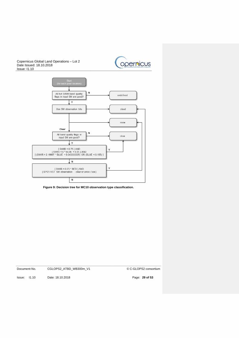
most optimal observations are used. The observation type is determined as shown in Figure 9. If
one or more radiometric bands quality flags in the S1-TOC SM show a bad quality, the new
observation type will be undefined. Next, the observation bits of the S1-TOC are taken into
account. If the observation of the S1-TOC is not ‘clear’, the observation is copied. The original
cloud detection of the PROBA-V collection 0 data, proved to do an under detection of clouds.
Hence, for each pixel with a ‘clear’ observation in the S1-TOC SM, an additional classification is
done base on the method of Vancutsemet al., 2007. The thresholds values have been adapted to
reflect the spectral difference between the SPOT-VGT 1km collection used in the reference
method and the PROBA-V 333m collection. To determine if the classified observation is a better
observation type or not, the following convention is used: clear observation pixels are considered
to be more optimal then snow. Snow pixels are considered to be more optimal then cloud pixels.
Cloud pixels are more optimal then undefined observation pixels. If for example the algorithm
would detect within a given dekad a total of 7 observations with 3 cloudy and 4 clear pixels, only
the latter 4 are used in the compositing. As such, only identical observation type pixels of the
most optimal type are accumulated in the sum and contribute to a second set of ‘number of
observations’, indicating the total observations of the most optimal observation type. This number
of observations (NMOD) is used to calculate the composite mean value.
Both NOBS and NMOD are stored in their own dataset in the MC10 file.
Commenté [BL7]: RID 1338

Copernicus Global Land Operations – Lot 2 Date Issued: 18.10.2018 Issue: I1.10
Document-No. CGLOPS2_ATBD_WB300m_V1
© C-GLOPS2 consortium
Issue: I1.10 Date: 18.10.2018 Page: 28 of 53
Figure 8: MC10 algorithm flow.
Copernicus Global Land Operations – Lot 2 Date Issued: 18.10.2018 Issue: I1.10
Document-No. CGLOPS2_ATBD_WB300m_V1
© C-GLOPS2 consortium
Issue: I1.10 Date: 18.10.2018 Page: 29 of 53
Figure 9: Decision tree for MC10 observation type classification.

Copernicus Global Land Operations – Lot 2 Date Issued: 18.10.2018 Issue: I1.10
Document-No. CGLOPS2_ATBD_WB300m_V1
© C-GLOPS2 consortium
Issue: I1.10 Date: 18.10.2018 Page: 30 of 53
Once all daily input data of a pixel is calculated, the status map is generated and the mean
composite value for all four spectral bands is calculated.
In addition to the mean reflectances for each band, the NMOD and the NOBS, the Mean
Compositing step also provides a status map (SM) (Table 7) for each pixel. The status map mimics
the bit positions as used in the PROBA-V input data Status Map.
Table 7: Status Map (SM) bit mapping.
Bit Name Description
1 -3 Observation
000: clear
010: undefined
011: cloud
100: snow/ice
4 Land/sea mask 0: sea
1: land
5 Mean composite SWIR quality flag 0: no mean composite
1: valid mean composite
6 Mean composite NIR quality flag 0: no mean composite
1: valid mean composite
7 Mean composite RED quality flag 0: no mean composite
1: valid mean composite
8 (Most
significant) Mean composite BLUE quality flag
0: no mean composite
1: valid mean composite
The observation status (bits 1 to 3) is based upon the most optimal observation used for the mean
composite.
The land/sea mask bit (bit 4) is an exact copy of the PROBA-V land/sea mask.
Bits 5, 6, 7 and 8 are quality flags for the mean composite spectral bands. The quality flag is set to
1 when a mean composite could be calculated and is set to 0 in case no compositing is done. The
latter only occurs when there was no valid observation to be used in the compositing (NMOD
equals 0).

Copernicus Global Land Operations – Lot 2 Date Issued: 18.10.2018 Issue: I1.10
Document-No. CGLOPS2_ATBD_WB300m_V1
© C-GLOPS2 consortium
Issue: I1.10 Date: 18.10.2018 Page: 31 of 53
3.2.7.2 Construction of the Water Bodies Potential Mask
This mask was derived from the GLSDEM, which has a 90 m horizontal and 1 m vertical resolution,
in three steps:
1. Search for the lowest points in the terrain.
A pixel is a candidate lowest point and a potential water body when the pixel elevation is lower
than or equal to its eight neighbours. Therefore, the 8 pixels neighbourhood of each GLSDEM
pixel is evaluated. Figure 10a shows part of the GLSDEM over the Rift Valley in Ethiopia, in
Figure 10b the detected lowest points are shown (in yellow).
Figure 10: a) Part of the 90 m spatial resolution GLSDEM over Rift Valley in Ethiopia. b) The detected
lowest points for this area are colored yellow. The larger sized colored areas are areas of equally low
elevation which correspond to some smaller lakes in the region.
2. Filtering and expanding the detected lowest points.
The next step in generating the WBPM is expanding the detected lowest points depending on the
topography. For each detected lowest point, an imaginary water level is raised in steps of 1m till
the maximum rise of 5m or the flooding1 condition is reached. As long as the edge of the potential
WB is not flooded, its area is extended according to the raised level, i.e. all neighbouring pixels
having the additional elevation are added to the potential WB area. This is schematically shown in
1 Flooding means detection of a pixel in the expanded area with an elevation lower than the actual rise level,
e.g. if the imaginary water level is raised to 405 m and there is a pixel in the expanded area which has an
elevation of 404 m, than the flooding condition is reached.

Copernicus Global Land Operations – Lot 2 Date Issued: 18.10.2018 Issue: I1.10
Document-No. CGLOPS2_ATBD_WB300m_V1
© C-GLOPS2 consortium
Issue: I1.10 Date: 18.10.2018 Page: 32 of 53
a two dimensional representation in Figure 11. The initial detected lowest point contains two pixels.
Rising the water level 1 m will expand the potential WB with an additional 5 pixels. Because no
flooding occurs the water level is increased again with 1 m. Now, 3 additional pixels are added to
the potential WB. Further, rising the water level will start flooding the WB because the first pixel
elevation right to the expanded WB is now lower. The pixels initially detected as lowest point and
surrounded by eight neighbours of equal height are marked as ”Level-1” in the potential WBs map.
The other initially detected lowest points and the expanded pixels are marked as “Level-2”. The
two levels are used in the last step when resizing the potential WBs map to the PROBA-V
resolution to obtain the final WBPM.
Figure 11: Expanding the initially detected lowest point by systematically rising an imaginary water
level in steps of 1 m. The corresponding 90 m spatial resolution pixels are indicated by the dots at
the bottom.
Figure 12 shows a detail from an area over Rift Valley. The horizontal and vertical profile plots are
taken according to the red lines in the images. The focus location of the plots is placed in the
center of a detected potential WB as shown by the crossing red lines in the detail images. In the
plots, this location is marked by the vertical red line. As seen in the detail window on the horizontal
profile, one additional potential WB was detected marked (1). On the vertical profile two additional
potential WBs were detected marked (1’) and (3).
Copernicus Global Land Operations – Lot 2 Date Issued: 18.10.2018 Issue: I1.10
Document-No. CGLOPS2_ATBD_WB300m_V1
© C-GLOPS2 consortium
Issue: I1.10 Date: 18.10.2018 Page: 33 of 53
Figure 12: a) Part of the GLSDEM over Rift Valley. b) The detected potential WBs for this area. The
detailed window shows a potential WB in the center (crossing of red lines). The horizontal and
vertical profiles are according to the red lines over the images. On the horizontal profile, the wetland
(1) near lake Hora (2) and the potential water body (indicated by the long red arrow) are seen. On the
vertical profile part of the wetland (1’) near lake Hora (2), the potential water body (indicated by the
long red arrow) and lake Bishoftu (3) are seen.
3. Deriving the WBPM
In the final step, the 90 m spatial resolution potential WBs map is re-sampled to the PROBA-V 300
m spatial resolution. For each pixel in the PROBA-V image, the corresponding pixels in the 90m
potential WBs map are located (which is 121 pixels). The resized (300 m) WBPM pixel is indicated
as a potential WB in two cases:
- At least one of the corresponding pixels was labelled as “Level-1”;
- At least nine of the corresponding pixels (7%, a figure empirically defined) were labelled as
“Level-2”.
Copernicus Global Land Operations – Lot 2 Date Issued: 18.10.2018 Issue: I1.10
Document-No. CGLOPS2_ATBD_WB300m_V1
© C-GLOPS2 consortium
Issue: I1.10 Date: 18.10.2018 Page: 34 of 53
Figure 13(a) shows a visual representation of the PROBA-V image over the Rift Valley test area
and the derived WBPM for the same area in (b). Indicated are the lakes Abijato and Langano. A
profile according to the red line is taken over the area for which the GLSDEM profile is shown in
the plot. The seven detected potential WBs over this profile are indicated by the transparent
colored boxes.
The WBPM was made based on the GLSDEM for which data was collected in the early 2000s.
Because of the high resolution of the GLSDEM dataset (90 m spatial and 1 m vertical), the derived
WBPM (300 m spatial resolution) reveals the finest detail as shown in Figure 13(b). Although the
Earth’s topography changes only notably over large geological time scales, natural events
(earthquakes) or anthropogenic activities (dam building) can influence the topography on shorter
time scales. Therefore, when such events take place, the WBPM needs to be updated.
The resulting 300 m WBPM (1=”potential water body”, 0=”no water body possible”) is used as an
extra input in the WB DETECTION processing step. The PROBA-V 300 m world image contains
120.960 samples x 47.040 lines or 5.7*109 pixels. Of those amount 29% (1.7*109 pixels) consists
of land mass (i.e. not ocean), 50.5% (833.3*106 pixels) of those land mass is indicated as potential
water body.

Copernicus Global Land Operations – Lot 2 Date Issued: 18.10.2018 Issue: I1.10
Document-No. CGLOPS2_ATBD_WB300m_V1
© C-GLOPS2 consortium
Issue: I1.10 Date: 18.10.2018 Page: 35 of 53
Figure 13: a) Part of image MC10_20131021 taken over the Rift Valley in Ethiopia (SWIR, NIR and Red
bands assigned to the RGB channels resp.). b) The WBPM for the same area in (a) (white=potential
water body, black=no water body possible). The plot shows the vertical GLSDEM profile according to
the red line. Marked with the blue boxes are the seven potential WBs. The arrows indicate the
location of lake Abijato (1) and lake Langano (2).
3.2.7.3 Colorimetric transformation
The Global Water Watch (GWW) algorithm (Pekel et al., 2005) was originally developed and
optimized for a window extending from Senegal (17.7° West) to India (85° East) and from the
equator to the Mediterranean sea (37.4°North) in the framework of the Global Watch project (Pekel
et al., 2005). Later on, the methodology was improved and adapted to MODIS and validated over
Africa (Pekel et al., 2014).
The approach is based on a transformation of the RGB (Red, Green and Blue) color space into
HSV (Hue, Saturation and Value) that decouples chromaticity and luminance (Figure 14). The HSV
color space is also commonly used in image processing. It is a nonlinear transformation of the
RGB color space using equations 1, 2 and 3 presented in Figure 14, with R mapped to SWIR
band, G to NIR band and B to the RED band. The Hue (H) is defined as the dominant wavelength

Copernicus Global Land Operations – Lot 2 Date Issued: 18.10.2018 Issue: I1.10
Document-No. CGLOPS2_ATBD_WB300m_V1
© C-GLOPS2 consortium
Issue: I1.10 Date: 18.10.2018 Page: 36 of 53
of the perceived color. It is the visual perceptual property corresponding to the categories called
yellow, blue, green, etc. Hue is considered as an angle between a reference line and the color
point, going from 0° to 360°. The Saturation (S) is defined as the degree of purity of the color and
may be intuitively considered as the amount of white mixed in a color. This component represents
the radial distance from the cone center going from 0 to 1. The nearer the point is to the center, the
lighter is the color. The Value (V), which is a brightness approximation, represents the height of the
axis of the HSV cone, going from 0 to 1. This axis describes the gray levels.
𝑉 = 𝑚𝑎𝑥(𝑅, 𝐺, 𝐵) (1)
𝑆 =𝑉−𝑚𝑖𝑛(𝑅,𝐺,𝐵)
𝑉 (2)
𝐻 =
{
(60° ∗
𝐺−𝐵
𝑉−𝑚𝑖𝑛(𝑅,𝐺,𝐵)+ 360°)𝑚𝑜𝑑 360° 𝑖𝑓 𝑉 = 𝑅
60° ∗𝐵−𝑅
𝑉−𝑚𝑖𝑛(𝑅,𝐺,𝐵)+ 120° 𝑖𝑓 𝑉 = 𝐺
60° ∗𝑅−𝐺
𝑉−𝑚𝑖𝑛(𝑅,𝐺,𝐵)+ 240° 𝑖𝑓 𝑉 = 𝐵
(3)
Figure 14: The HSV color space.
This color space presents three interesting properties: (i) it is intuitive as it represents the colors as
interpreted by human brain; (ii) the chromaticity (H and S) and Value (V) are decoupled, reducing
the problem of brightness level inconsistencies of the pixel perceived color (i.e. spatially and
temporally) resulting from various observation conditions. This property is fundamental, as the
automatic detection technique has to be independent of all effects affecting the received spectral
signal. Practically, a way to solve this issue is to collapse the 3-dimensional space into a 2-
dimensional sub-space keeping only the Hue and Value components of the perceived color.
Among the 2 components, (iii) H represents a qualitative spectral index.
By analyzing the distribution of the pixels in the Hue - Value space, the pixels can be classified as
“water” and as “no water” based on thresholds (see Pekel et al., 2014).

Copernicus Global Land Operations – Lot 2 Date Issued: 18.10.2018 Issue: I1.10
Document-No. CGLOPS2_ATBD_WB300m_V1
© C-GLOPS2 consortium
Issue: I1.10 Date: 18.10.2018 Page: 37 of 53
3.2.7.4 Invalid data filtering
Figure 15: The first part of the WBDA comprises invalid data filtering.
The first part of the Water Body Detection Algorithm (WBDA) comprises invalid data filtering
(Figure 15). The status of each image pixel is defined by the Status Map of MC10. Pixels indicated
as “undefined” in the MC10 Status Map are classified here as “No Data”.
A low sun elevation causes elongated shadows which are observed in the remote sensing imagery
as darkened Earth surfaces. These might be detected as water bodies when their VALUE drops
below the threshold level. A check on the Solar Zenith Angle (SZA) prohibits the detection of
invalid WBs, i.e. when a pixel has a SZA larger than 65° no WB detection is done and the pixel is
classified as “No Data”.
The next step in the WBDA is filtering the clouds, the cloud shadows and snow, using the
information from the MC10 Status Map. Pixels indicated as “Cloud” or “Snow” are not considered in
the WB detection algorithm.
Cloud shadows on the Earth’s surface often cause the VALUE to drop below the threshold and are
as such regularly classified as WBs. Therefore, to avoid confusion due to cloud shadow in the
immediate neighbourhood of the initial defined cloud pixel, an additional dilate filtering is
performed. In case a pixel is indicated as “Cloud” in the MC10 status map, its surrounding twelve
neighbouring pixels (the circular neighbourhood with radius 2 pixels, i.e. they total twelve pixels)
are considered as “Cloud” as well and are therefore not taken into account for WB detection.
Figure 16 shows the result of cloud shadow masking over two locations in Argentina having a dark
soil background (a, b). Before cloud dilation was performed numerous false detected water bodies
can be seen (b,d). These false detections are caused by the cloud’s shadow. The cloud dilatation,
by a circular neighbourhood of twelve pixels around the cloud pixels, most false detections are
prohibited. The circular neighbourhood of twelve pixels was empirical defined and is a trade-off
between commission and omission errors (c,f).
Commenté [BL8]: RID 1389
Copernicus Global Land Operations – Lot 2 Date Issued: 18.10.2018 Issue: I1.10
Document-No. CGLOPS2_ATBD_WB300m_V1
© C-GLOPS2 consortium
Issue: I1.10 Date: 18.10.2018 Page: 38 of 53
Figure 16: The removal of cloud shadow by dilatation of the cloud indicated pixels. a) Dekad
MC10_20140511 over Argentina (center at 31°33’50”S, 65°10’37”W). b) The Water Bodies detection
result without delate filtering. Due to cloud shadows lots of false WB detections appear. c) After de
clouds are dilated by its circular neighborhood of twelve pixels most of the false detections are
masked by the dilated cloud. The red oval shows a false detection which could not be reached by the
dilated cloud. d) Dekad MC10_20140511 over Argentina (center at 31°45’58”S, 65°4’44”W). e) An
existing small lake is shown in the lower left part of the image, besides some false detections can be
seen near to the clouds. No cloud dilatation was done yet. f) After cloud dilatation the false detection
don’t appear, a small part of the lake is now obstructed by the dilated cloud as indicated by the red
oval.
Copernicus Global Land Operations – Lot 2 Date Issued: 18.10.2018 Issue: I1.10
Document-No. CGLOPS2_ATBD_WB300m_V1
© C-GLOPS2 consortium
Issue: I1.10 Date: 18.10.2018 Page: 39 of 53
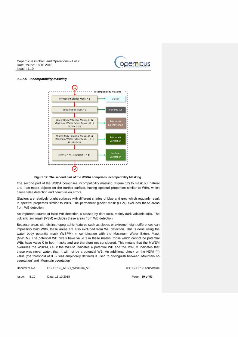
3.2.7.5 Incompatibility masking
Figure 17: The second part of the WBDA comprises Incompatibility Masking.
The second part of the WBDA comprises incompatibility masking (Figure 17) to mask out natural
and man-made objects on the earth’s surface, having spectral properties similar to WBs, which
cause false detection and commission errors.
Glaciers are relatively bright surfaces with different shades of blue and grey which regularly result
in spectral properties similar to WBs. The permanent glacier mask (PGM) excludes these areas
from WB detection.
An important source of false WB detection is caused by dark soils, mainly dark volcanic soils. The
volcanic soil mask (VSM) excludes these areas from WB detection.
Because areas with distinct topographic features such as slopes or extreme height differences can
impossibly hold WBs, these areas are also excluded from WB detection. This is done using the
water body potential mask (WBPM) in combination with the Maximum Water Extent Mask
(MWEM). The potential WB pixels have value 1 in these masks; those which cannot be potential
WBs have value 0 in both masks and are therefore not considered. This means that the MWEM
overrules the WBPM, i.e. if the WBPM indicates a potential WB and the MWEM indicates that
these was never water, than it will not be a potential WB. An additional check on the NDVI (4)
value (the threshold of 0.32 was empirically defined) is used to distinguish between ‘Mountain no
vegetation’ and ‘Mountain vegetation’.
Copernicus Global Land Operations – Lot 2 Date Issued: 18.10.2018 Issue: I1.10
Document-No. CGLOPS2_ATBD_WB300m_V1
© C-GLOPS2 consortium
Issue: I1.10 Date: 18.10.2018 Page: 40 of 53
𝑁𝐷𝑉𝐼 = 𝜌𝑁𝐼𝑅−𝜌𝑅𝐸𝐷
𝜌𝑁𝐼𝑅+𝜌𝑅𝐸𝐷 (4)
Finally, vegetated surfaces, e.g. large overhanging trees or floating plants, prohibit the detection of
WBs underneath. Besides, vegetated surfaces often cause confusion with WBs. Therefore, the
NDVI is used to identify the vegetated areas. Pixels having an NDVI value higher or equal to 0.32
(the threshold was empirically defined) and having a WBPM pixel set (locating lowland areas
where holding a WB is possible) are considered to be “Lowland Vegetation”.
Some WBs have a high NDVI value (due to algae load or adjacency effect of the surrounding
vegetation) and are as such classified as “Lowland Vegetation”. To avoid these omission errors an
additional check on VALUE is added, this threshold level is denoted as NV. If the VALUE of a pixel
which is designated as “Lowland Vegetation”, is less than 0.11 (a value empirically defined) it is
considered as “Water” depending on the thresholds of HUE and VALUE.
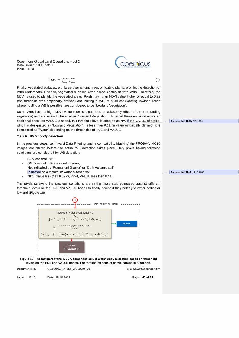
3.2.7.6 Water body detection
In the previous steps, i.e. ‘Invalid Data Filtering’ and ‘Incompatibility Masking’ the PROBA-V MC10
images are filtered before the actual WB detection takes place. Only pixels having following
conditions are considered for WB detection:
- SZA less than 65°;
- SM does not indicate cloud or snow;
- Not indicated as “Permanent Glacier” or “Dark Volcanic soil”
- Indicated as a maximum water extent pixel;
- NDVI value less than 0.32 or, if not, VALUE less than 0.11.
The pixels surviving the previous conditions are in the finals step compared against different
threshold levels on the HUE and VALUE bands to finally decide if they belong to water bodies or
lowland (Figure 18)
Figure 18: The last part of the WBDA comprises actual Water Body Detection based on threshold
levels on the HUE and VALUE bands. The thresholds consist of two parabolic functions.
Commenté [BL9]: RID 1333
Commenté [BL10]: RID 1336
Copernicus Global Land Operations – Lot 2 Date Issued: 18.10.2018 Issue: I1.10
Document-No. CGLOPS2_ATBD_WB300m_V1
© C-GLOPS2 consortium
Issue: I1.10 Date: 18.10.2018 Page: 41 of 53
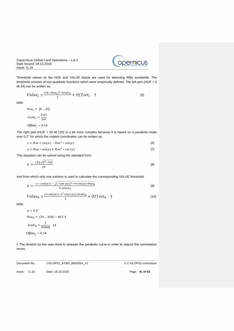
Threshold values on the HUE and VALUE bands are used for detecting WBs worldwide. The
threshold consists of two quadratic functions which were empirically defined. The left part (HUE = 0
till 34) can be written as:
𝑉𝑎𝑙𝑢𝑒𝐿 ≤(34−𝐻𝑢𝑒𝐿)
2∗𝑆𝑐𝑎𝑙𝑒𝐿
2+ 𝑂𝑓𝑓𝑠𝑒𝑡𝐿 † (5)
With:
𝐻𝑢𝑒𝐿 = [0…34]
𝑆𝑐𝑎𝑙𝑒𝐿 =0.41
342
14.0=LOffset
The right part (HUE = 34 till 120) is a bit more complex because it is based on a parabola rotate
over 0.2° for which the rotated coordinates can be written as:
𝑥 = 𝐻𝑢𝑒 ∗ cos(𝛼) − 𝐻𝑢𝑒2 ∗ 𝑠𝑖𝑛(𝛼) (6)
𝑦 = 𝐻𝑢𝑒 ∗ 𝑠𝑖𝑛(𝛼) + 𝐻𝑢𝑒2 ∗ cos (𝛼) (7)
This equation can be solved using the standard form:
𝑥 =−𝑏±√𝑏2−4𝑎𝑐
2𝑎 (8)
And from which only one solution is used to calculate the corresponding VALUE threshold:
𝑥 =−(−cos(𝛼)) − √(−cos (𝛼))2−4∗𝑠𝑖𝑛(𝛼)∗𝐻𝑢𝑒𝑅
2∗𝑠𝑖𝑛(𝛼) (9)
𝑉𝑎𝑙𝑢𝑒𝑅 ≤(𝑥∗𝑠𝑖𝑛(𝛼)+ 𝑥2∗cos (𝛼))∗𝑆𝑐𝑎𝑙𝑒𝑅
2+ 𝑂𝑓𝑓𝑠𝑒𝑡𝑅 † (10)
With:
𝛼 = 0.2°
𝐻𝑢𝑒𝑅 = [34…360] − 48.5 ‡
𝑆𝑐𝑎𝑙𝑒𝑅 =1
95000 ‡‡
14.0=ROffset
† The division by two was done to sharpen the parabolic curve in order to reduce the commission
errors.
Copernicus Global Land Operations – Lot 2 Date Issued: 18.10.2018 Issue: I1.10
Document-No. CGLOPS2_ATBD_WB300m_V1
© C-GLOPS2 consortium
Issue: I1.10 Date: 18.10.2018 Page: 42 of 53
‡ The value 48.5 was empirically defined; it is used to broaden the parabolic curve (higher values
will broaden the curve).
‡‡ The value 95000 in the scale factor was empirically defined; it defines the height of the
parabolic curve (higher values will lower the curve).
The parabolic thresholds consists of a left and a right part. The OffsetL and OffsetR directly
influence the “minimum level” of the parabolic function. They must at all times have identical values
otherwise there will be a ‘jump’ in the function. The maximum HUE is always in the right part and is
contained in the HueR parameter. This one immediately defines the max HUE value. In other
words these parameters directly define the shape and level of the parabolic function as inherent
defined by the math functions.
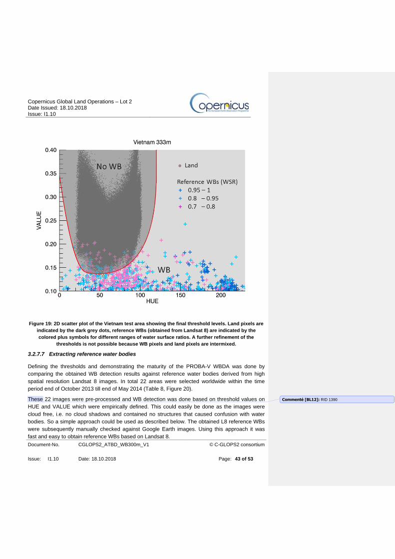
Figure 19 shows the 2D scatter plots of the Vietnam test areas. The 2D scatter plot has the HUE
on the x-axis and VALUE on the y-axis. The location of the pixels from the reference WBs are
indicated by the colored plus symbols and this for three ranges of Water Surface Ratio (WSR), i.e.
blue for WSR = 0.95 to 1, cyan for WSR = 0.8 to 0.95 and magenta for WSR = 0.7 to 0.8. The
other WSR ranges are not indicated as they would overrule the figure. The non-WB pixels, which
are denoted as land, are indicated by the dark grey dot symbols. The final thresholds levels are
indicated by the red lines. Although the final thresholds are tuned to detect as much WBs as
possible, not all WBs can be detected because they are intermixed with land pixels.
Commenté [BL11]: RID 1330
Copernicus Global Land Operations – Lot 2 Date Issued: 18.10.2018 Issue: I1.10
Document-No. CGLOPS2_ATBD_WB300m_V1
© C-GLOPS2 consortium
Issue: I1.10 Date: 18.10.2018 Page: 43 of 53
Figure 19: 2D scatter plot of the Vietnam test area showing the final threshold levels. Land pixels are
indicated by the dark grey dots, reference WBs (obtained from Landsat 8) are indicated by the
colored plus symbols for different ranges of water surface ratios. A further refinement of the
thresholds is not possible because WB pixels and land pixels are intermixed.
3.2.7.7 Extracting reference water bodies
Defining the thresholds and demonstrating the maturity of the PROBA-V WBDA was done by
comparing the obtained WB detection results against reference water bodies derived from high
spatial resolution Landsat 8 images. In total 22 areas were selected worldwide within the time
period end of October 2013 till end of May 2014 (Table 8, Figure 20).
These 22 images were pre-processed and WB detection was done based on threshold values on
HUE and VALUE which were empirically defined. This could easily be done as the images were
cloud free, i.e. no cloud shadows and contained no structures that caused confusion with water
bodies. So a simple approach could be used as described below. The obtained L8 reference WBs
were subsequently manually checked against Google Earth images. Using this approach it was
fast and easy to obtain reference WBs based on Landsat 8.
Commenté [BL12]: RID 1390

Copernicus Global Land Operations – Lot 2 Date Issued: 18.10.2018 Issue: I1.10
Document-No. CGLOPS2_ATBD_WB300m_V1
© C-GLOPS2 consortium
Issue: I1.10 Date: 18.10.2018 Page: 44 of 53
Table 8: Landsat-8 scenes used to define the PROBA-V water bodies detection thresholds.
Figure 20: Location of the Landsat scenes used to define the detection method.
Landsat 8 scene Dekad Lat Lon ns nl
1 Argentina1 LC82270862014111LGN00 20140421 -36.40625000 -63.94196429 299 239
2 Argentina2 LC82310932014011LGN00 20140111 -46.29910714 -73.83482143 376 257
3 Australia LC81110782014131LGN00 20140511 -24.94196429 118.49553571 267 236
4 Bangladesh LC81380442014112LGN00 20140421 24.17410714 87.74553571 244 240
5 Bolivia LC82330692013310LGN00 20131101 -11.95089286 -66.85267857 232 239
6 Brazil LC82220742014028LGN00 20140121 -19.17410714 -51.55803571 248 237
7 Canada LC80180272014151LGN00 20140521 48.53125000 -80.06696429 332 246
8 China LC81210382014121LGN00 20140501 32.79910714 116.05803571 271 240
9 Congo LC81740662014140LGN00 20140521 -7.62053571 25.22767857 235 238
10 India LC81460422014072LGN00 20140311 27.04910714 76.05803571 249 240
11 Mali LC81950502013332LGN00 20131121 15.51339286 -2.25446429 234 239
12 Mexico LC80270422014118LGN00 20140421 27.04017857 -100.12053571 260 238
13 Poland LC81870222014087LGN00 20140401 55.60267857 21.60267857 393 250
14 RiftValley1 LC81680542013335LGN00 20131201 9.72767857 38.20089286 232 238
15 RiftValley2 LC81680552013335LGN00 20131201 8.28125000 37.89732143 231 238
16 RiftValley3 LC81680562013335LGN00 20131201 6.83482143 37.59375000 230 238
17 Rusia LC81770212014129LGN00 20140501 56.99553571 37.60267857 426 248
18 SouthAfrica LC81690802014121LGN00 20140501 -27.77232143 28.12946429 277 246
19 Spain LC82010332014121LGN00 20140501 39.95089286 -5.66517857 306 239
20 Turkey LC81730332013306LGN00 20131101 39.95982143 37.65625000 299 240
21 USA LC80430342014134LGN00 20140511 38.54017857 -121.87946429 281 242
22 Vietnam LC81240512014062LGN00 20140301 14.08482143 107.11160714 241 242
SPOT-VGTUpper Left CoordinateN° Area
2013/ 14
Copernicus Global Land Operations – Lot 2 Date Issued: 18.10.2018 Issue: I1.10
Document-No. CGLOPS2_ATBD_WB300m_V1
© C-GLOPS2 consortium
Issue: I1.10 Date: 18.10.2018 Page: 45 of 53
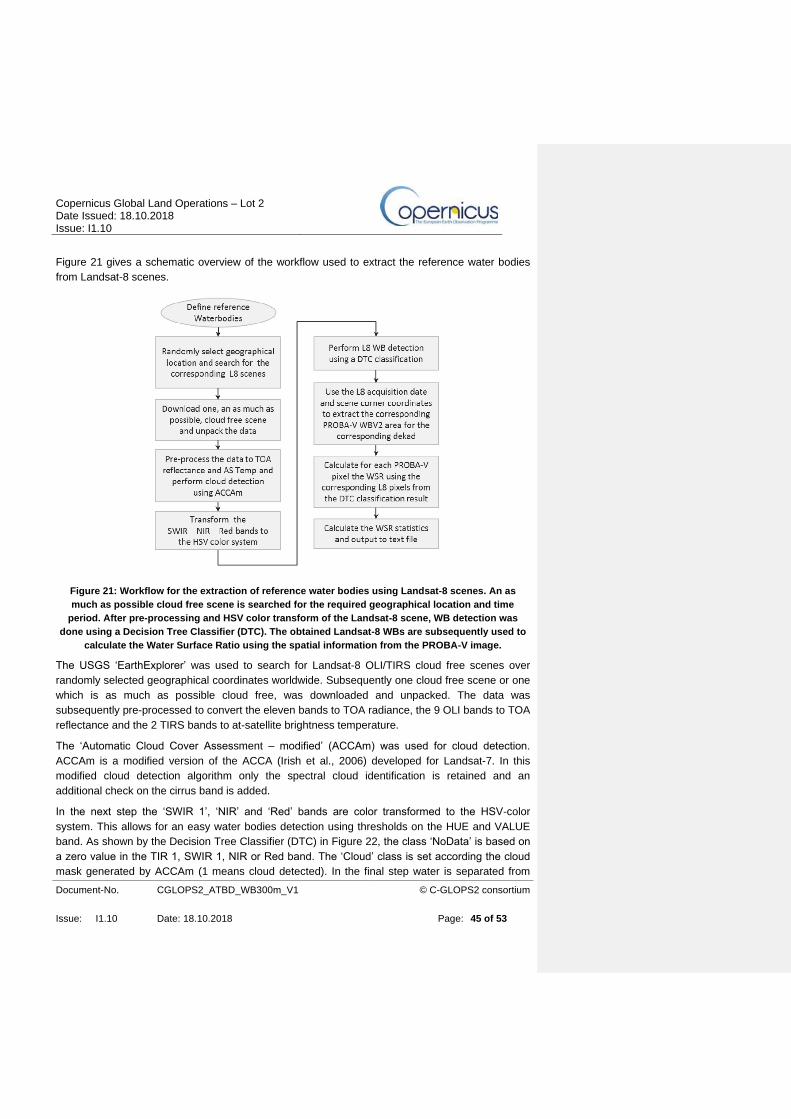
Figure 21 gives a schematic overview of the workflow used to extract the reference water bodies
from Landsat-8 scenes.
Figure 21: Workflow for the extraction of reference water bodies using Landsat-8 scenes. An as
much as possible cloud free scene is searched for the required geographical location and time
period. After pre-processing and HSV color transform of the Landsat-8 scene, WB detection was
done using a Decision Tree Classifier (DTC). The obtained Landsat-8 WBs are subsequently used to
calculate the Water Surface Ratio using the spatial information from the PROBA-V image.
The USGS ‘EarthExplorer’ was used to search for Landsat-8 OLI/TIRS cloud free scenes over
randomly selected geographical coordinates worldwide. Subsequently one cloud free scene or one
which is as much as possible cloud free, was downloaded and unpacked. The data was
subsequently pre-processed to convert the eleven bands to TOA radiance, the 9 OLI bands to TOA
reflectance and the 2 TIRS bands to at-satellite brightness temperature.
The ‘Automatic Cloud Cover Assessment – modified’ (ACCAm) was used for cloud detection.
ACCAm is a modified version of the ACCA (Irish et al., 2006) developed for Landsat-7. In this
modified cloud detection algorithm only the spectral cloud identification is retained and an
additional check on the cirrus band is added.
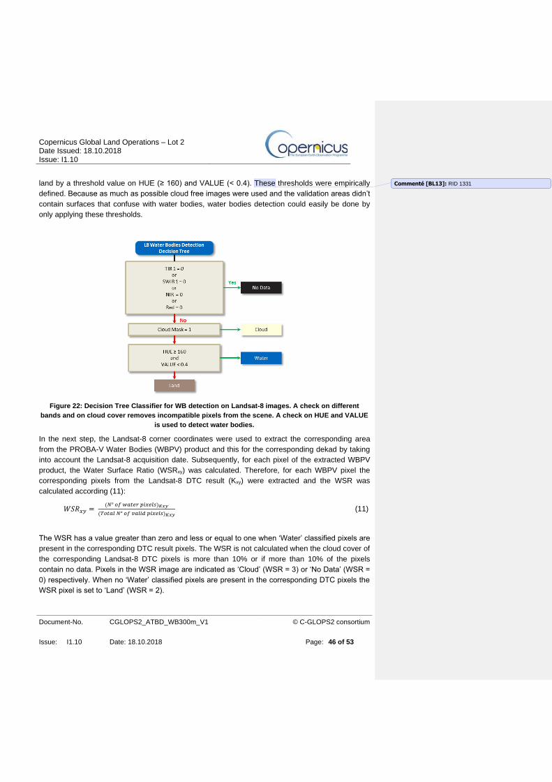
In the next step the ‘SWIR 1’, ‘NIR’ and ‘Red’ bands are color transformed to the HSV-color
system. This allows for an easy water bodies detection using thresholds on the HUE and VALUE
band. As shown by the Decision Tree Classifier (DTC) in Figure 22, the class ‘NoData’ is based on
a zero value in the TIR 1, SWIR 1, NIR or Red band. The ‘Cloud’ class is set according the cloud
mask generated by ACCAm (1 means cloud detected). In the final step water is separated from
Copernicus Global Land Operations – Lot 2 Date Issued: 18.10.2018 Issue: I1.10
Document-No. CGLOPS2_ATBD_WB300m_V1
© C-GLOPS2 consortium
Issue: I1.10 Date: 18.10.2018 Page: 46 of 53
land by a threshold value on HUE (≥ 160) and VALUE (< 0.4). These thresholds were empirically
defined. Because as much as possible cloud free images were used and the validation areas didn’t
contain surfaces that confuse with water bodies, water bodies detection could easily be done by
only applying these thresholds.
Figure 22: Decision Tree Classifier for WB detection on Landsat-8 images. A check on different
bands and on cloud cover removes incompatible pixels from the scene. A check on HUE and VALUE
is used to detect water bodies.
In the next step, the Landsat-8 corner coordinates were used to extract the corresponding area
from the PROBA-V Water Bodies (WBPV) product and this for the corresponding dekad by taking
into account the Landsat-8 acquisition date. Subsequently, for each pixel of the extracted WBPV
product, the Water Surface Ratio (WSRxy) was calculated. Therefore, for each WBPV pixel the
corresponding pixels from the Landsat-8 DTC result (Kxy) were extracted and the WSR was
calculated according (11):
𝑊𝑆𝑅𝑥𝑦 = (𝑁° 𝑜𝑓 𝑤𝑎𝑡𝑒𝑟 𝑝𝑖𝑥𝑒𝑙𝑠)𝐾𝑥𝑦
(𝑇𝑜𝑡𝑎𝑙 𝑁° 𝑜𝑓 𝑣𝑎𝑙𝑖𝑑 𝑝𝑖𝑥𝑒𝑙𝑠)𝐾𝑥𝑦 (11)
The WSR has a value greater than zero and less or equal to one when ‘Water’ classified pixels are
present in the corresponding DTC result pixels. The WSR is not calculated when the cloud cover of
the corresponding Landsat-8 DTC pixels is more than 10% or if more than 10% of the pixels
contain no data. Pixels in the WSR image are indicated as ‘Cloud’ (WSR = 3) or ‘No Data’ (WSR =
0) respectively. When no ‘Water’ classified pixels are present in the corresponding DTC pixels the
WSR pixel is set to ‘Land’ (WSR = 2).
Commenté [BL13]: RID 1331
Copernicus Global Land Operations – Lot 2 Date Issued: 18.10.2018 Issue: I1.10
Document-No. CGLOPS2_ATBD_WB300m_V1
© C-GLOPS2 consortium
Issue: I1.10 Date: 18.10.2018 Page: 47 of 53
In the final step a confusion matrix (CMX) is calculated as described by Roy and Boschetti (2009)
and Padila et al. 2014. From these CMX the overall accuracy (OA), commission error (CE) and
omission error (OE) is calculated. The OE is calculated per minimum WSR range (WSRm), i.e.
0.95, 0.8, 0.7, 0.6 and 0.5 and per test area.
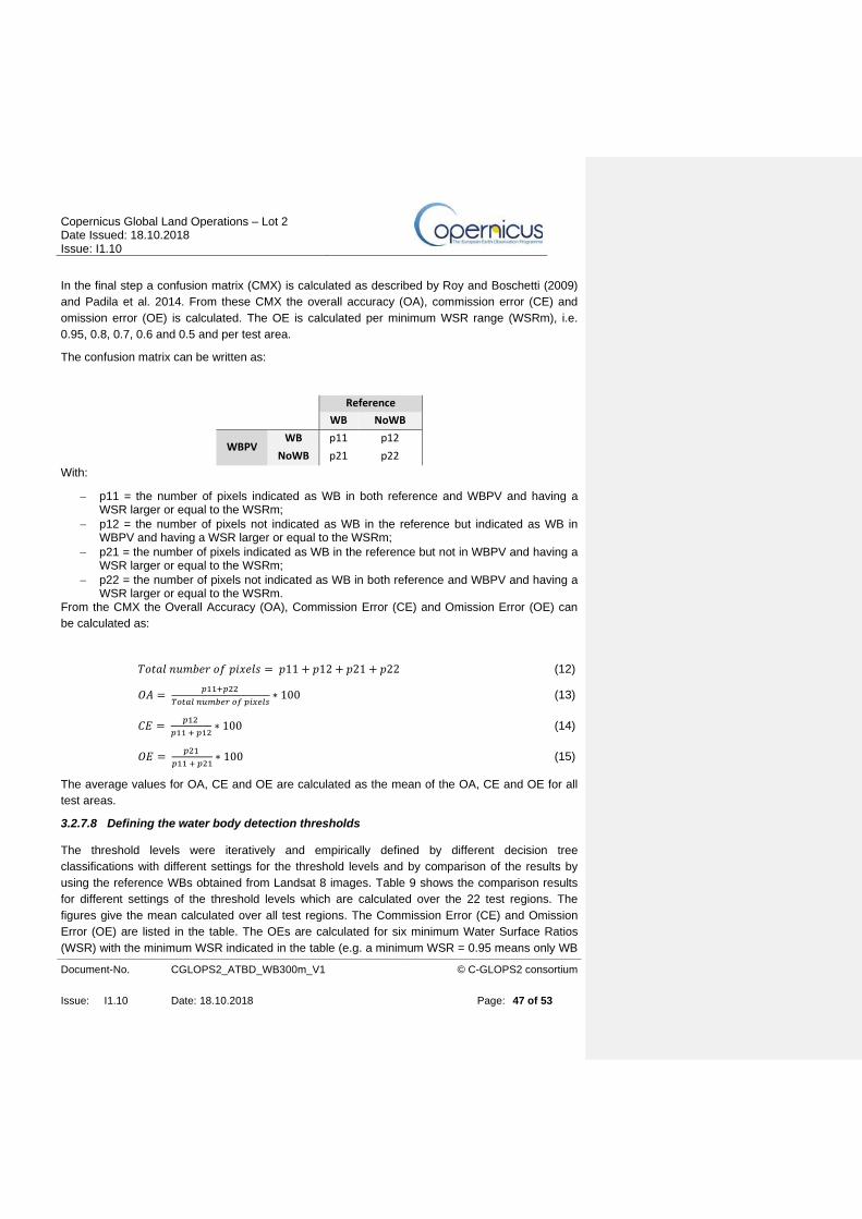
The confusion matrix can be written as:
Reference
WB NoWB
WBPV WB p11 p12
NoWB p21 p22
With:
− p11 = the number of pixels indicated as WB in both reference and WBPV and having a WSR larger or equal to the WSRm;
− p12 = the number of pixels not indicated as WB in the reference but indicated as WB in WBPV and having a WSR larger or equal to the WSRm;
− p21 = the number of pixels indicated as WB in the reference but not in WBPV and having a WSR larger or equal to the WSRm;
− p22 = the number of pixels not indicated as WB in both reference and WBPV and having a WSR larger or equal to the WSRm.
From the CMX the Overall Accuracy (OA), Commission Error (CE) and Omission Error (OE) can
be calculated as:
𝑇𝑜𝑡𝑎𝑙 𝑛𝑢𝑚𝑏𝑒𝑟 𝑜𝑓 𝑝𝑖𝑥𝑒𝑙𝑠 = 𝑝11 + 𝑝12 + 𝑝21 + 𝑝22 (12)
𝑂𝐴 = 𝑝11+𝑝22
𝑇𝑜𝑡𝑎𝑙 𝑛𝑢𝑚𝑏𝑒𝑟 𝑜𝑓 𝑝𝑖𝑥𝑒𝑙𝑠∗ 100 (13)
𝐶𝐸 = 𝑝12
𝑝11 + 𝑝12∗ 100 (14)
𝑂𝐸 = 𝑝21
𝑝11 + 𝑝21∗ 100 (15)
The average values for OA, CE and OE are calculated as the mean of the OA, CE and OE for all
test areas.
3.2.7.8 Defining the water body detection thresholds
The threshold levels were iteratively and empirically defined by different decision tree
classifications with different settings for the threshold levels and by comparison of the results by
using the reference WBs obtained from Landsat 8 images. Table 9 shows the comparison results
for different settings of the threshold levels which are calculated over the 22 test regions. The
figures give the mean calculated over all test regions. The Commission Error (CE) and Omission
Error (OE) are listed in the table. The OEs are calculated for six minimum Water Surface Ratios
(WSR) with the minimum WSR indicated in the table (e.g. a minimum WSR = 0.95 means only WB
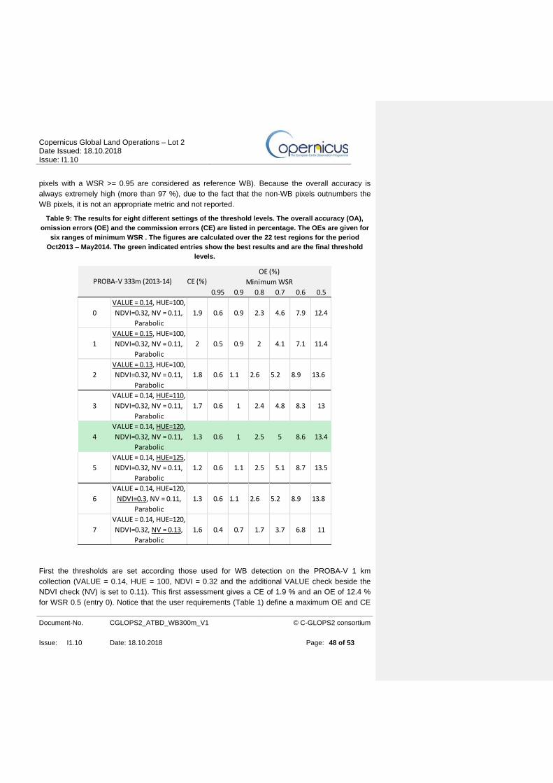
Copernicus Global Land Operations – Lot 2 Date Issued: 18.10.2018 Issue: I1.10
Document-No. CGLOPS2_ATBD_WB300m_V1
© C-GLOPS2 consortium
Issue: I1.10 Date: 18.10.2018 Page: 48 of 53
pixels with a WSR >= 0.95 are considered as reference WB). Because the overall accuracy is
always extremely high (more than 97 %), due to the fact that the non-WB pixels outnumbers the
WB pixels, it is not an appropriate metric and not reported.
Table 9: The results for eight different settings of the threshold levels. The overall accuracy (OA),
omission errors (OE) and the commission errors (CE) are listed in percentage. The OEs are given for
six ranges of minimum WSR . The figures are calculated over the 22 test regions for the period
Oct2013 – May2014. The green indicated entries show the best results and are the final threshold
levels.
First the thresholds are set according those used for WB detection on the PROBA-V 1 km
collection (VALUE = 0.14, HUE = 100, NDVI = 0.32 and the additional VALUE check beside the
NDVI check (NV) is set to 0.11). This first assessment gives a CE of 1.9 % and an OE of 12.4 %
for WSR 0.5 (entry 0). Notice that the user requirements (Table 1) define a maximum OE and CE
0.95 0.9 0.8 0.7 0.6 0.5
0
VALUE = 0.14, HUE=100,
NDVI=0.32, NV = 0.11,
Parabolic
1.9 0.6 0.9 2.3 4.6 7.9 12.4
1
VALUE = 0.15, HUE=100,
NDVI=0.32, NV = 0.11,
Parabolic
2 0.5 0.9 2 4.1 7.1 11.4
2
VALUE = 0.13, HUE=100,
NDVI=0.32, NV = 0.11,
Parabolic
1.8 0.6 1.1 2.6 5.2 8.9 13.6
3
VALUE = 0.14, HUE=110,
NDVI=0.32, NV = 0.11,
Parabolic
1.7 0.6 1 2.4 4.8 8.3 13
4
VALUE = 0.14, HUE=120,
NDVI=0.32, NV = 0.11,
Parabolic
1.3 0.6 1 2.5 5 8.6 13.4
5
VALUE = 0.14, HUE=125,
NDVI=0.32, NV = 0.11,
Parabolic
1.2 0.6 1.1 2.5 5.1 8.7 13.5
6
VALUE = 0.14, HUE=120,
NDVI=0.3, NV = 0.11,
Parabolic
1.3 0.6 1.1 2.6 5.2 8.9 13.8
7
VALUE = 0.14, HUE=120,
NDVI=0.32, NV = 0.13,
Parabolic
1.6 0.4 0.7 1.7 3.7 6.8 11
PROBA-V 333m (2013-14) CE (%)
OE (%)
Minimum WSR
Copernicus Global Land Operations – Lot 2 Date Issued: 18.10.2018 Issue: I1.10
Document-No. CGLOPS2_ATBD_WB300m_V1
© C-GLOPS2 consortium
Issue: I1.10 Date: 18.10.2018 Page: 49 of 53
of 15%. The VALUE threshold is subsequently increased to 0.15 which results in an increased CE
(entry 1), and decreased to 0.13 which results in increased OEs (entry 2). Because the CE or OE
errors increase, these settings were not retained. Increasing the HUE threshold to 110 and 120
(entry 3 and 4 vs entry 0) decreases the commission error with a slight increase of omission error.
Further increasing the HUE threshold to 125 (entry 5) slightly improves the commission error but
also the omission errors increases and therefore this option was not retained. Subsequently the
NDVI threshold was decreased to 0.3 (entry 6 vs entry 4) resulting in both increased CE and OEs.
Finally the NV value was increased showing better OEs, however the CE increased (entry 7 vs
entry 4). The last two settings were therefore not retained, so the final settings are according entry
4, which are identical to the settings for the PROBA-V 1 km collection except for the HUE threshold
which is increased to 120.
3.2.7.9 Water body occurrence estimation
To qualify the occurrence of the detected WBs, a Water Body Occurrence (WBO) is calculated for
each detected WB pixel in each dekad. This measure gives an idea about the permanency or
seasonality of the detected WBs. The WBO is added as a Quality Layer (QUAL) in the final output
product. To obtain a WBO map for each dekad, per pixel statistics are calculated by temporal-
sequential processing of the available dekads. If more than sixty-four2 cloud free MC10 composite
observations are available, only the last 64 cloud free observations including the actual observation
are used for calculating the statistics. This means that for the first dekads (observation started Oct.
2013) there are none or only a few dekads available for statistics.
The per-pixel temporal-sequential statistics are calculated over the available observation dekads
(max 64) and can be summarized as:
− Total number of temporal cloud free observations (ntObs)*
− Total number of temporal WB detections (ntWBs)
− Maximum number of continuous temporal WB detections (mctWBs)
* Note that after some time when many dekads are available ntObs will become fixed to 64.
From these statistics, the frequency of detected WBs can be calculated as:
( )( )
( )%100ntObsnsobservatiolcloudfreeroftemporaTotalnumbe
ntWBsonslWBdetectiroftemporaTotalnumbe=WBf (16)
As shown in Figure 23, the calculated WB frequency (WBf) and the maximum number of
continuous temporal WB detections (mctWBs) can be visualized in a 2D scatter plot which, in his
turn, is used for defining the occurrence threshold levels. The different occurrence levels are
2 To get an idea of the WB occurrence the observation period over which the statistics are calculated has to be long enough. An observation period over two years requires 72 dekads. However, for computational reason only 64 dekads are observed, information which can be stored in one “long word” (64 bits). This can be justified by the fact that per pixel not each dekad holds valid data due to cloud or cloud shadow, snow or an invalid SZA. This results in an observation period for most, if not all, of the pixels of more than 2 years.
Copernicus Global Land Operations – Lot 2 Date Issued: 18.10.2018 Issue: I1.10
Document-No. CGLOPS2_ATBD_WB300m_V1
© C-GLOPS2 consortium
Issue: I1.10 Date: 18.10.2018 Page: 50 of 53
indicated by the different colored regions in the figure. The slope and position of the four threshold
lines, marked L, M, H and VH, define the WBO threshold levels and are designed as such in the
first phase. These thresholds were defined independently of the calibration areas. They were
merely defined by common sense reasoning, i.e. WBs that appear with a high frequency (WBf) or
with long continuous observation periods (mctWBs) are most likely stable WBs that exist for a
longer period and therefore have a higher occurrence than those with lower frequency (WBf) of
shorter continuous observation periods (mctWBs). The advantage of defining the thresholds in this
way is that they can be easily adapted if needed. The defined occurrence threshold levels can be
expressed as:
𝑉𝑒𝑟𝑦 𝐿𝑜𝑤 = (𝑚𝑐𝑡𝑊𝐵𝑠 > 0) & (𝑚𝑐𝑡𝑊𝐵𝑠 < (2 + 𝛼𝐿 ∗𝑊𝐵𝑓)) (17)
𝐿𝑜𝑤 = (𝑚𝑐𝑡𝑊𝐵𝑠 ≥ (2 + 𝛼𝐿 ∗ 𝑊𝐵𝑓)) & (𝑚𝑐𝑡 𝑊𝐵𝑠 < (3 + 𝛼𝑀 ∗𝑊𝐵𝑓)) (18)
𝑀𝑒𝑑𝑖𝑢𝑚 = (𝑚𝑐𝑡𝑊𝐵𝑠 ≥ (3 + 𝛼𝑀 ∗𝑊𝐵𝑓)) & (𝑚𝑐𝑡 𝑊𝐵𝑠 < (4 + 𝛼𝐻 ∗ 𝑊𝐵𝑓)) (19)
𝐻𝑖𝑔ℎ = (𝑚𝑐𝑡𝑊𝐵𝑠 ≥ (4 + 𝛼𝐻 ∗ 𝑊𝐵𝑓)) & (𝑚𝑐𝑡 𝑊𝐵𝑠 < (5 + 𝛼𝑉𝐻 ∗𝑊𝐵𝑓)) (20)
𝑉𝑒𝑟𝑦 𝐻𝑖𝑔ℎ = 𝑚𝑐𝑡𝑊𝐵𝑠 ≥ (5 + 𝛼𝑉𝐻 ∗ 𝑊𝐵𝑓) (21)
𝑃𝑒𝑟𝑚𝑎𝑛𝑒𝑛𝑡 = 𝑊𝐵𝑓 ≥ 95 (22)
Where αx is the slope of the threshold line x, e.g.
𝛼𝑉𝐻 =5−0
0−60 (23)
The red line (o1) shows the minimum WBf in relation to the mctWBs. The slope depends on the
maximum number of observations (ntObs) made which in this case is thirty-one3 when all dekads
have valid data.
The plot shows that a certain pixel is classified as a ‘Very High’ WBO if it is identified as WB in at
least five consecutive dekads (point ‘m’ in the plot). Note that this number is independent of the
ntObs. As an example, if a pixel was detected as a WB in three consecutive dekads (with nObs =
31) its WBf will be 9.7 % and therefore will have a WBO “Medium” (point “a”). If this pixel would
have subsequently four additional WB detections in separate single dekads its WBf will rise to 22.6
% and its WBO will increase to “High” (point “b”).
Note also that if pixels have a WBf of at least 95% their WBO will be “Permanent”.
3 31 MC10 images were used, from 21 Oct. 2013 till 21 Aug. 2014.
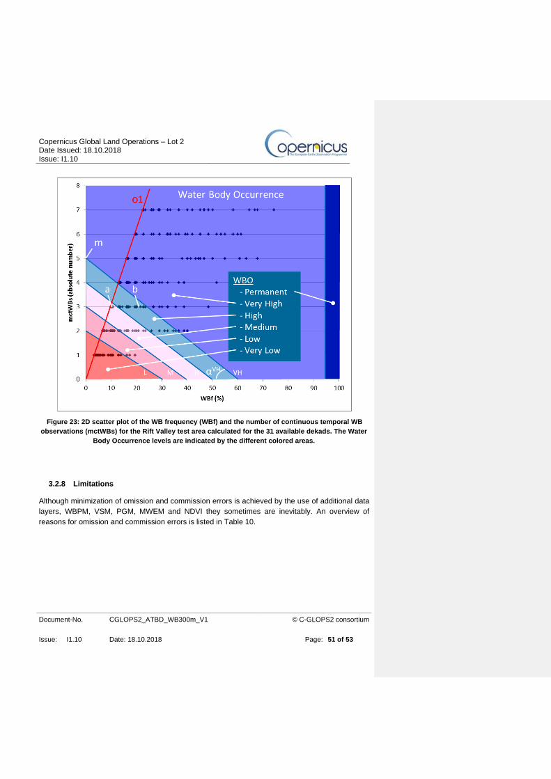
Copernicus Global Land Operations – Lot 2 Date Issued: 18.10.2018 Issue: I1.10
Document-No. CGLOPS2_ATBD_WB300m_V1
© C-GLOPS2 consortium
Issue: I1.10 Date: 18.10.2018 Page: 51 of 53
Figure 23: 2D scatter plot of the WB frequency (WBf) and the number of continuous temporal WB
observations (mctWBs) for the Rift Valley test area calculated for the 31 available dekads. The Water
Body Occurrence levels are indicated by the different colored areas.
3.2.8 Limitations
Although minimization of omission and commission errors is achieved by the use of additional data
layers, WBPM, VSM, PGM, MWEM and NDVI they sometimes are inevitably. An overview of
reasons for omission and commission errors is listed in Table 10.

Copernicus Global Land Operations – Lot 2 Date Issued: 18.10.2018 Issue: I1.10
Document-No. CGLOPS2_ATBD_WB300m_V1
© C-GLOPS2 consortium
Issue: I1.10 Date: 18.10.2018 Page: 52 of 53
Table 10: Omission and commission errors are caused by several reasons.
Omission errors due to:
1 Small sized WBs in the order of the size of one PROBA-V pixel;
2 WBs with spectral properties that fall outside the defined thresholds;
3 New WBs not covered by the MWEM (32 years, 1984-2015).
Commission errors due to:
1 Cloud shadow caused by thin undetected clouds especially over dark dense vegetation and in mountainous areas;
2 Dark soils especially volcanic soils (which are not masked by the VSM);
3 Dark areas caused by anthropogenic activity, e.g. heavy industry;
4 Dark areas caused by shadow, e.g. high buildings in large cities;
5 Anthropogenic structures with spectral signatures equal to WBs, e.g. some agricultural fields, build-up areas;
6 Natural surfaces with spectral signatures very close to WBs, e.g. salt lakes;
To minimize confusion the user should use the product with attention to the QUAL which reflects
the history of detected WBs.
3.3 QUALITY ASSESSMENT
See CGLOPS2_QAR_WB300m_V1 upon public release.
3.4 RISK OF FAILURE AND MITIGATION MEASURES
In case the quality of the PROBA-V sensor degrades, the spectral response correction needs to be
adapted and the defined thresholds for Water Body detection need to be updated if necessary.
Copernicus Global Land Operations – Lot 2 Date Issued: 18.10.2018 Issue: I1.10
Document-No. CGLOPS2_ATBD_WB300m_V1
© C-GLOPS2 consortium
Issue: I1.10 Date: 18.10.2018 Page: 53 of 53
4 REFERENCES
GCOS-200 (2016). Systematic Observation Requirements for Satellite-based Products for Climate
Supplemental details to the satellite-based component of the Implementation Plan for the
Global Observing System for Climate in Support of the UNFCCC - 2016 Update, WMO,
Geneva, Switzerland. http://www.wmo.int/pages/prog/gcos/Publications/gcos-200.pdf
Irish, R. R., Barker, J. L., Goward, S. N., & Arvidson, T. J., (2006). Characterization of the Landsat-
7 ETM Automated Cloud-Cover Assessment (ACCA) algorithm. Photogrammetric
Engineering & Remote Sensing, 72, 1179−1188.
NSIDC (2014): Global Land Ice Measurements from Space (GLIMS) glacier database. Compiled
and made available by the international GLIMS community and the National Snow and Ice
Data Center, Boulder CO, U.S.A. (DOI:10.7265/N5V98602).
http://glims.colorado.edu/glacierdata/
Pekel, J.-F., Bogaert, P., Adans, S., Rasson, J. P., & Defourny, P., (2005). STEREO : GlobalWatch
- Détection, Traitement automatique de séries temporelles optiques pour la cartographie et la
et la détection de changement. Intermediary report n°2 (Vol. Intermedia).
Pekel, J.-F., Vancutsem, C., Bastin, L., Clerici, M., Vanbogaert, E., Bartholomé, E., & Defourny, P.,
(2014). A near real-time water surface detection method based on HSV transformation of
MODIS multi-spectral time series data. Remote Sensing of Environment, 140, 704–716.
(doi:10.1016/j.rse.2013.10.008)
Pekel, J.-F., Cottam, A., Gorelick, N., Belward, A.S., (2016). High-resolution mapping of global
surface water and its long-term changes. Nature 540, 418-422. (doi:10.1038/nature20584)
Rahman, H. and Dedieu, G., (1994). SMAC: a simplified method for the atmospheric correction of
satellite measurements in the solar spectrum. International Journal of Remote Sensing,
15(1): 123-143
Roy, D.P.; Boschetti, L. Southern Africa validation of the MODIS, L3JRC, and GlobCarbon burned-
area products. IEEE Trans. Geosci. Remote Sens. 2009, 47, 1032–1044
USGS (2008), GLSDEM, 90m scene GLSDEM_p123r024_utmz13, Global Land Cover Facility,
University of Maryland, College Park, Maryland. (http://glcf.umd.edu/data/glsdem/)
Vancutsem, C., Pekel, J.‐F., Bogaert, P., & Defourny, P. (2007). Mean Compositing, an alternative
strategy for producing temporal syntheses. Concepts and performance assessment for
SPOT VEGETATION time series. International Journal of Remote Sensing, 28(22), 5123–
5141. doi:10.1080/01431160701253212
Commenté [BL14]: RID 1391