coordinated control of multiple uavs: theory and flight

HAL Id: hal-01061122https://hal-onera.archives-ouvertes.fr/hal-01061122

Submitted on 5 Sep 2014

HAL is a multi-disciplinary open accessarchive for the deposit and dissemination of sci-entific research documents, whether they are pub-lished or not. The documents may come fromteaching and research institutions in France orabroad, or from public or private research centers.

L’archive ouverte pluridisciplinaire HAL, estdestinée au dépôt et à la diffusion de documentsscientifiques de niveau recherche, publiés ou non,émanant des établissements d’enseignement et derecherche français ou étrangers, des laboratoirespublics ou privés.

Coordinated Control of Multiple UAVs : Theory andFlight Experiment.

Y. Watanabe

To cite this version:Y. Watanabe. Coordinated Control of Multiple UAVs : Theory and Flight Experiment.. AIAA Guid-ance Navigation & Control (GNC) Conference, Aug 2013, BOSTON, United States. �hal-01061122�

https://hal-onera.archives-ouvertes.fr/hal-01061122

https://hal.archives-ouvertes.fr

Coordinated Control of Multiple UAVs :

Theory and Flight Experiment

Yoko Watanabe∗∗

ONERA - The French Aerospace Laboratory, Toulouse 31055, France

This paper proposes a nonlinear control law to realize a coordinated flight of multipleUAVs and evaluates its performance through flight experiments of small fixed-wing UAVplatforms. Assuming all-to-all communication, a decentralized coordination control systemis designed based on a virtual leader approach. The proposed control design uses a po-tential function defined on a phase distribution of multi agents. Two advantages of thiscoordination controller are; i) it can be applied to make different coordination configura-tions, ii) it is applicable to any number of UAVs, and so it can easily treat an event ofaddition/deletion of UAV units in a coordination team. The proposed coordination controllaw is proven to be locally asymptotically stable by using Lyapunov indirect method, andits large domain of attraction is observed in simulation. Furthermore, the controller is im-plemented onboard ONERA fixed-wing UAV platforms and tested with a mission scenariowhich includes four different coordination configurations.

I. Introduction

Coordinated operation of multiple unmanned aerial vehicles (UAVs) has aroused many researchers’ in-terest in recent years, due to its great potential for increases in overall mission performance and robustnesswithout augmenting a capacity of each UAV unit. The followings are some examples showing advantages ofmulti-UAV operation over mono-UAV one. For a surveillance mission, even though each vehicle can carrya limited number/type of sensors, data fusion of several of them distributed over an operation site in adesired configuration can provide further information and a wider sensing coverage. Communication relaycan be established between vehicles to extend a range of datalink connection with a ground control station.System robustness can be improved by making redundancy so that a functional failure of one UAV amonga team does not necessarily lead a mission failure. There is also an aerodynamic benefit to reduce a powerconsumption of each aircraft when flying in formation1.

Various strategies for multi-agent coordination have been investigated in robotics community since manyyears. Especially, formation control of multiple robots, aircrafts, underwater vehicles or satellites has beenintensively studied2. There are two objectives in a coordination control problem. One is to make each agentmaintain a desired geometric configuration with respect to others. The other is to make an entire teamachieve a mission objective such as reference trajectory tracking. Two main approaches for such coordinationcontrol are i) leader-follower approach and ii) virtual structure approach. In the leader-follower approach, anagent designated as a leader takes charge of a mission objective and the other agents designated as followersmaintain a desired configuration with respect to the leader. A big advantage of using this approach lies inits facility of implementation. As shown in Figure 1, the leader-follower coordination control architecturedoes not have any feedback loop from followers to the leader (C and D blocks in the figure denote a localcontroller and an agent dynamics respectively, for each agent.). This is why most of the existing work ofsuccessful UAV formation flight adopt this approach. Bayraktar et al.3 and Dong et al.4 realized a formationflight between two fixed-wing airplanes and between two helicopters respectively, by updating a follower’sflight plan using a current leader’s position in real-time on ground control station. In the work of Gu et al.5,three airplanes flew in formation by transmitting a leader’s position directly to the two followers by radiocommunication. Johnson et al.6 developed a vision-based system onboard a follower aircraft to localize a

∗Research Engineer, Systems Control and Flight Dynamics Department, [email protected]

1 of 25

American Institute of Aeronautics and Astronautics

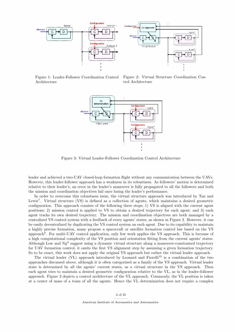
Figure 1: Leader-Follower Coordination ControlArchitecture

Figure 2: Virtual Structure Coordination Con-trol Architecture

Figure 3: Virtual Leader-Follower Coordination Control Architecture

leader and achieved a two-UAV closed-loop formation flight without any communication between the UAVs.However, this leader-follower approach has a weakness in its robustness. As followers’ motion is determinedrelative to their leader’s, an error in the leader’s maneuver is fully propagated to all the followers and boththe mission and coordination objectives fail once losing the leader’s performance.

In order to overcome this robustness issue, the virtual structure approach was introduced by Tan andLewis7. Virtual structure (VS) is defined as a collection of agents, which maintains a desired geometricconfiguration. This approach consists of the following three steps; 1) VS is aligned with the current agentpositions; 2) mission control is applied to VS to obtain a desired trajectory for each agent; and 3) eachagent tracks its own desired trajectory. The mission and coordination objectives are both managed by acentralized VS control system with a feedback of every agents’ states, as shown in Figure 2. However, it canbe easily decentralized by duplicating the VS control system on each agent. Due to its capability to maintaina highly precise formation, many propose a spacecraft or satellite formation control law based on the VSapproach8. For multi-UAV control application, only few work applies the VS approach. This is because ofa high computational complexity of the VS position and orientation fitting from the current agents’ states.Although Low and Ng9 suggest using a dynamic virtual structure along a maneuver-constrained trajectoryfor UAV formation control, it omits the first VS alignment step by assuming a given formation trajectory.So to be exact, this work does not apply the original VS approach but rather the virtual leader approach.

The virtual leader (VL) approach introduced by Leonard and Fiorelli10 is a combination of the twoapproaches discussed above, although it is often categorized as a family of the VS approach. Virtual leaderstate is determined by all the agents’ current states, as a virtual structure in the VS approach. Theneach agent tries to maintain a desired geometric configuration relative to the VL, as in the leader-followerapproach. Figure 3 depicts a control architecture of the VL approach. Commonly, the VL position is takenat a center of mass of a team of all the agents. Hence the VL determination does not require a complex

2 of 25


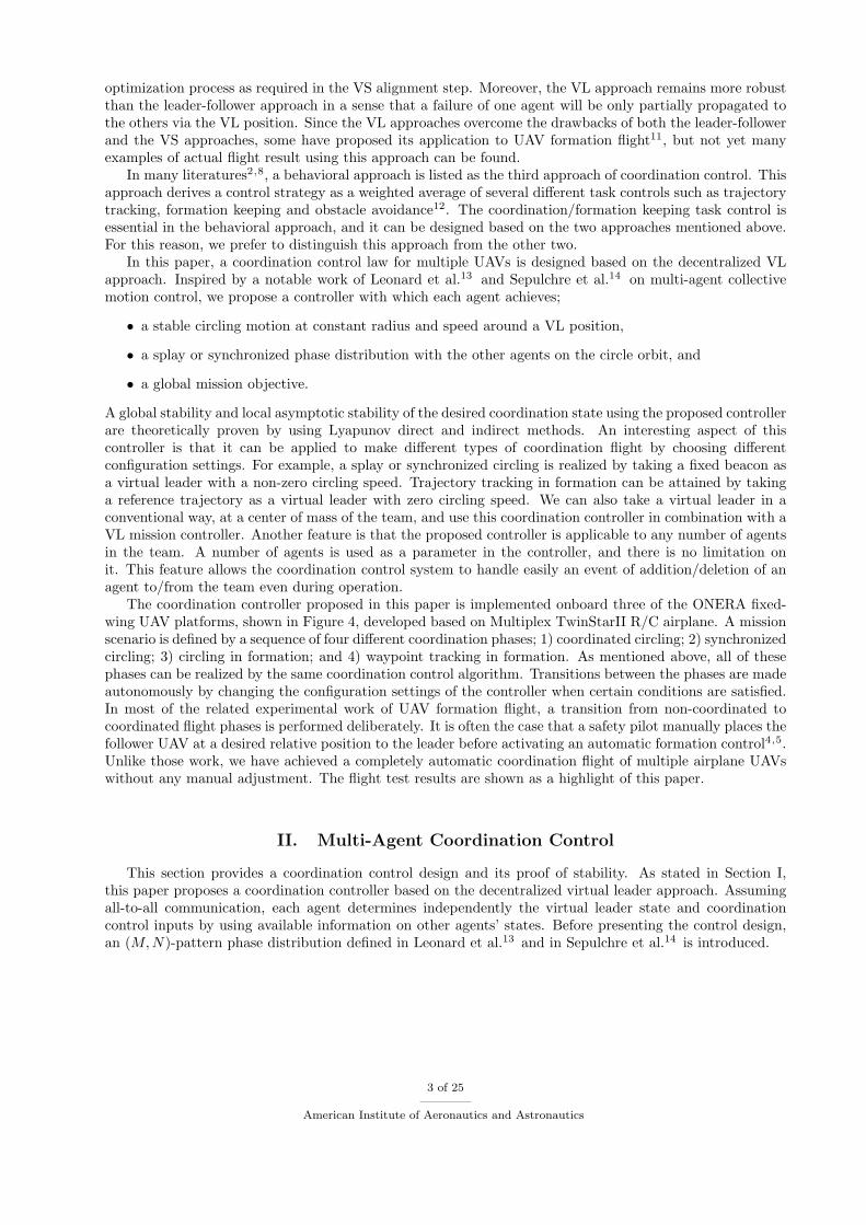
optimization process as required in the VS alignment step. Moreover, the VL approach remains more robustthan the leader-follower approach in a sense that a failure of one agent will be only partially propagated tothe others via the VL position. Since the VL approaches overcome the drawbacks of both the leader-followerand the VS approaches, some have proposed its application to UAV formation flight11, but not yet manyexamples of actual flight result using this approach can be found.

In many literatures2,8, a behavioral approach is listed as the third approach of coordination control. Thisapproach derives a control strategy as a weighted average of several different task controls such as trajectorytracking, formation keeping and obstacle avoidance12. The coordination/formation keeping task control isessential in the behavioral approach, and it can be designed based on the two approaches mentioned above.For this reason, we prefer to distinguish this approach from the other two.

In this paper, a coordination control law for multiple UAVs is designed based on the decentralized VLapproach. Inspired by a notable work of Leonard et al.13 and Sepulchre et al.14 on multi-agent collectivemotion control, we propose a controller with which each agent achieves;

• a stable circling motion at constant radius and speed around a VL position,

• a splay or synchronized phase distribution with the other agents on the circle orbit, and

• a global mission objective.

A global stability and local asymptotic stability of the desired coordination state using the proposed controllerare theoretically proven by using Lyapunov direct and indirect methods. An interesting aspect of thiscontroller is that it can be applied to make different types of coordination flight by choosing differentconfiguration settings. For example, a splay or synchronized circling is realized by taking a fixed beacon asa virtual leader with a non-zero circling speed. Trajectory tracking in formation can be attained by takinga reference trajectory as a virtual leader with zero circling speed. We can also take a virtual leader in aconventional way, at a center of mass of the team, and use this coordination controller in combination with aVL mission controller. Another feature is that the proposed controller is applicable to any number of agentsin the team. A number of agents is used as a parameter in the controller, and there is no limitation onit. This feature allows the coordination control system to handle easily an event of addition/deletion of anagent to/from the team even during operation.

The coordination controller proposed in this paper is implemented onboard three of the ONERA fixed-wing UAV platforms, shown in Figure 4, developed based on Multiplex TwinStarII R/C airplane. A missionscenario is defined by a sequence of four different coordination phases; 1) coordinated circling; 2) synchronizedcircling; 3) circling in formation; and 4) waypoint tracking in formation. As mentioned above, all of thesephases can be realized by the same coordination control algorithm. Transitions between the phases are madeautonomously by changing the configuration settings of the controller when certain conditions are satisfied.In most of the related experimental work of UAV formation flight, a transition from non-coordinated tocoordinated flight phases is performed deliberately. It is often the case that a safety pilot manually places thefollower UAV at a desired relative position to the leader before activating an automatic formation control4,5.Unlike those work, we have achieved a completely automatic coordination flight of multiple airplane UAVswithout any manual adjustment. The flight test results are shown as a highlight of this paper.

II. Multi-Agent Coordination Control

This section provides a coordination control design and its proof of stability. As stated in Section I,this paper proposes a coordination controller based on the decentralized virtual leader approach. Assumingall-to-all communication, each agent determines independently the virtual leader state and coordinationcontrol inputs by using available information on other agents’ states. Before presenting the control design,an (M,N)-pattern phase distribution defined in Leonard et al.13 and in Sepulchre et al.14 is introduced.

3 of 25


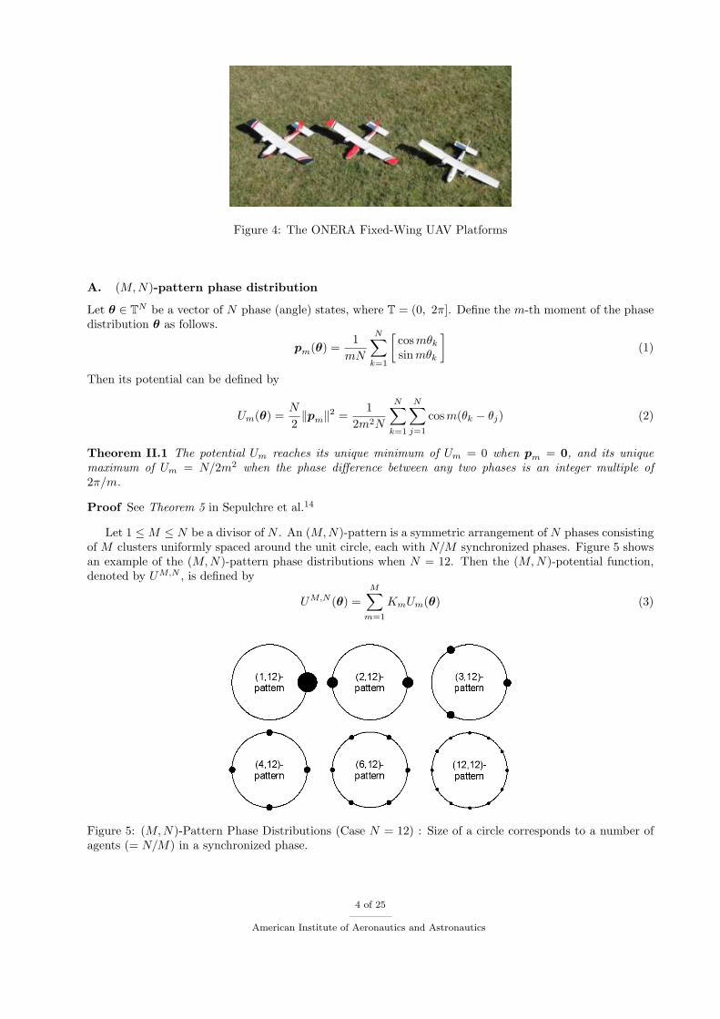
Figure 4: The ONERA Fixed-Wing UAV Platforms

A. (M,N)-pattern phase distribution

Let θ ∈ TN be a vector of N phase (angle) states, where T = (0, 2π]. Define the m-th moment of the phasedistribution θ as follows.

pm(θ) =1

mN

N∑

k=1

[cosmθk

sin mθk

](1)

Then its potential can be defined by

Um(θ) =N

2‖pm‖2 =

12m2N

N∑

k=1

N∑

j=1

cosm(θk − θj) (2)

Theorem II.1 The potential Um reaches its unique minimum of Um = 0 when pm = 0, and its uniquemaximum of Um = N/2m2 when the phase difference between any two phases is an integer multiple of2π/m.

Proof See Theorem 5 in Sepulchre et al.14

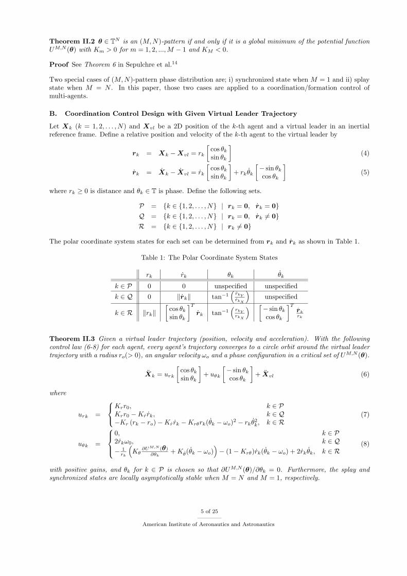
Let 1 ≤ M ≤ N be a divisor of N . An (M, N)-pattern is a symmetric arrangement of N phases consistingof M clusters uniformly spaced around the unit circle, each with N/M synchronized phases. Figure 5 showsan example of the (M, N)-pattern phase distributions when N = 12. Then the (M, N)-potential function,denoted by UM,N , is defined by

UM,N (θ) =M∑

m=1

KmUm(θ) (3)

Figure 5: (M,N)-Pattern Phase Distributions (Case N = 12) : Size of a circle corresponds to a number ofagents (= N/M) in a synchronized phase.

4 of 25


Theorem II.2 θ ∈ TN is an (M,N)-pattern if and only if it is a global minimum of the potential functionUM,N (θ) with Km > 0 for m = 1, 2, ...,M − 1 and KM < 0.

Proof See Theorem 6 in Sepulchre et al.14

Two special cases of (M,N)-pattern phase distribution are; i) synchronized state when M = 1 and ii) splaystate when M = N . In this paper, those two cases are applied to a coordination/formation control ofmulti-agents.

B. Coordination Control Design with Given Virtual Leader Trajectory

Let Xk (k = 1, 2, . . . , N) and Xvl be a 2D position of the k-th agent and a virtual leader in an inertialreference frame. Define a relative position and velocity of the k-th agent to the virtual leader by

rk = Xk −Xvl = rk

[cos θk

sin θk

](4)

rk = Xk − Xvl = rk

[cos θk

sin θk

]+ rkθk

[− sin θk

cos θk

](5)

where rk ≥ 0 is distance and θk ∈ T is phase. Define the following sets.

P = {k ∈ {1, 2, . . . , N} | rk = 0, rk = 0}Q = {k ∈ {1, 2, . . . , N} | rk = 0, rk 6= 0}R = {k ∈ {1, 2, . . . , N} | rk 6= 0}

The polar coordinate system states for each set can be determined from rk and rk as shown in Table 1.

Table 1: The Polar Coordinate System States

rk rk θk θk

k ∈ P 0 0 unspecified unspecified

k ∈ Q 0 ‖rk‖ tan−1(

rkY

rkX

)unspecified

k ∈ R ‖rk‖[

cos θk

sin θk

]T

rk tan−1(

rkY

rkX

) [− sin θk

cos θk

]Trk

rk

Theorem II.3 Given a virtual leader trajectory (position, velocity and acceleration). With the followingcontrol law (6-8) for each agent, every agent’s trajectory converges to a circle orbit around the virtual leadertrajectory with a radius ro(> 0), an angular velocity ωo and a phase configuration in a critical set of UM,N (θ).

Xk = urk

[cos θk

sin θk

]+ uθk

[− sin θk

cos θk

]+ Xvl (6)

where

urk =

Krr0, k ∈ PKrr0 −Kr rk, k ∈ Q−Kr (rk − ro)−Kr rk −Krθrk(θk − ωo)2 − rkθ2

k, k ∈ R(7)

uθk =

0, k ∈ P2rkω0, k ∈ Q− 1

rk

(Kθ

∂UM,N (θ)∂θk

+ Kθ(θk − ωo))− (1−Krθ)rk(θk − ωo) + 2rkθk, k ∈ R

(8)

with positive gains, and θk for k ∈ P is chosen so that ∂UM,N (θ)/∂θk = 0. Furthermore, the splay andsynchronized states are locally asymptotically stable when M = N and M = 1, respectively.

5 of 25


Proof With the controller (6-8), the relative distance dynamics of the k-th agent become

rk =

Krr0, k ∈ PKrr0 −Kr rk, k ∈ Q−Kr (rk − ro)−Kr rk −Krθrk(θk − ωo)2, k ∈ R

The relative phase dynamics are not specified for k ∈ P, θk = ω0 for k ∈ Q, and

θk = − 1r2k

(Kθ

∂UM,N (θ)∂θk

+ Kθ(θk − ωo))− (1−Krθ)

rk

rk(θk − ωo)

for k ∈ R. Define the system state by

x =

rrθθ

where r = [ r1 · · · rN ]T and θ = [ θ1 · · · θN ]T , and its domain by D = (R+N × RN × TN × RN ). Thedynamic system of the state x has the following limit cycle.

{rk = r0, rk = 0, θk = ω0 ∀ k ∈ {1, 2, ..., N}θ of an (M,N)-pattern phase distribution

(9)

Define a potential function as below.

V M,N (x) =1

2Kθ

N∑

k=1

{Kr (rk − ro)

2 + r2k + r2

k(θk − ωo)2}

+ UM,N (θ) (10)

where UM,N (θ) defined in (3). This function is lower-bounded by KMN/2M2, which is attained uniquelyat the limit cycle (9). A time-derivative of this potential function V M,N (x) is derived as follows.

V M,N (x) =N∑

k=1

θk∂UM,N (θ)

∂θk+

Kr

Kθ

N∑

k=1

(rk − ro) rk +1

Kθ

N∑

k=1

(rk(rk + rk(θk − ωo)2) + r2

k(θk − ωo)θk

)

= −Kr

Kθ

∑

k/∈Pr2k −

Kθ

Kθ

∑

k∈R(θk − ωo)2 + ω0

∑

k/∈P

∂UM,N (θ)∂θk

+∑

k∈Pθk

∂UM,N (θ)∂θk

The last two terms vanish as

∂UM,N (θ)∂θk

= 0 for ∀ k ∈ P,∑

k/∈P

∂UM,N (θ)∂θk

=N∑

k=1

∂UM,N (θ)∂θk

= 0

Hence, we have

V M,N (x) = −Kr

Kθ

∑

k/∈Pr2k −

Kθ

Kθ

∑

k∈R(θk − ωo)2 ≤ 0 (11)

In result, the potential function V M,N (x) defined in (10) is a Lyapunov function and the limit cycle (9) isstable. Let S be a set of all points in the system domain where V M,N (x) = 0, i.e.,

S ={

x ∈ D ∣∣ rk = 0 for ∀k, θk = ω0 for ∀k /∈ P}

(12)

A point in an invariant set in S first needs to satisfy rk = 0 for ∀k, which implies rk = r0 for ∀k (and hencethe sets P and Q are null). At the same time, it also needs to satisfy θk = 0 for ∀k, which implies the criticalset of the (M,N)-potential function UM,N (θ). Therefore, the largest invariant set in S can be given by

M ={

x ∈ S∣∣ rk = r0,

∂UM,N (θ)∂θk

= 0 for ∀k}

6 of 25


From LaSalle’s invariant set theorem15, every trajectory starting in D approaches to the invariant set M.In other words,

rk → r0, rk → 0, θk → ω0 for ∀ k ∈ {1, 2, ..., N}and the phase configuration θ converges to one in the critical set of UM,N (θ) as t →∞.

Now we prove an asymptotical stability of the splay and synchronized state by using Lyapunov indirectmethod. Let δx be a small disturbance from the state in the limit cycle (9)) denoted by

x∗ =

r010θ∗

ω01

where 1 =

1...1

, 0 =

0...0

, θ∗ =

θ∗1...

θ∗N

Then its dynamics can be linearized as below.

δx = F (θ∗)δx =

O I O O−KrI −KrI O O

O O O IO O −Kθ

r20

A(θ∗) −Kθ

r20

I

δx (13)

where (i, j)-element of the matrix A(θ∗) in (13) is defined by

Aij(θ∗) =∂2UM,N (θ)

∂θi∂θj

∣∣∣θ=θ∗

= β∗ij − α∗i δij ,i = 1, 2, . . . , Nj = 1, 2, . . . , N

where δij is the Kronecker delta and

α∗i =1N

M∑m=1

Km

N∑

k=1

cos m(θ∗k − θ∗i ), β∗ij =1N

M∑m=1

Km cosm(θ∗j − θ∗i )

Note that, since β∗ij = β∗ji, the matrix A(θ∗) is symmetric and so has N real eigenvalues denoted byλAj (j = 1, 2, . . . , N). The matrix F (θ∗) has eigenvalues at

λr± =−Kr ±

√K2

r − 4Kr

2(14)

with multiplicity N associated with the relative distance dynamics, and also at

λθj± =−Kθ ±

√K2

θ− 4r2

0KθλAj

2r20

, j = 1, 2, . . . , N (15)

with multiplicity 1 associated with the phase dynamics. The eigenvalues λr± have a strictly negative realpart for any Kr > 0 and Kr > 0. Recall that λAj is real. A real part of λθj− is strictly negative for anyKθ > 0 and Kθ > 0. A real part of λθj+ is strictly positive for λAj < 0, zero for λAj = 0 and strictlynegative for λAj > 0. Consider the cases of θ∗ being the splay and the synchronized state.

i) Splay state (M = N) : Without loss of generality, the splay phase distribution can be representedas θ∗k = 2πk/N for k = 1, 2, . . . , N . With this θ∗, the matrix A(θ∗) becomes a cyclic matrix given by

A(θ∗) =

c0 c1 · · · cN−2 cN−1

cN−1 c0 c1 cN−2

... cN−1 c0. . .

...

c2. . . . . . c1

c1 c2 · · · cN−1 c0

where

c0 =1N

N∑m=1

Km −KN , ci =1N

N∑m=1

Km cos mi2π

N, i = 1, 2, . . . , N − 1

7 of 25


This cyclic matrix has the following eigenvalues and eigenvectors16.

λAj =N−1∑

k=0

ckeijk 2πN (16)

vAj = [ 1 eij 2πN ei2j 2π

N . . . ei(N−1)j 2πN ]T (17)

for j = 1, 2, . . . , N . By substituting ck into (16), λAj is expanded as follows.

λAj = c0 +1N

N−1∑

k=1

N∑m=1

Km cosmk2π

Ncos jk

2π

N

= c0 +1

2N

N−1∑

k=1

N∑m=1

Km cos (m + j)k2π

N+

12N

N−1∑

k=1

N∑m=1

Km cos (m− j)k2π

N

= c0 +1

2N

N∑

l=1

(Kl + Kl)

(N∑

k=1

cos lk2π

N− 1

)

where

Kl ={

N + l − j, 1 ≤ l ≤ jl − j, j + 1 ≤ l ≤ N

, Kl ={−l + j, 1 ≤ l ≤ j − 1

N − l + j, j ≤ l ≤ N

As we haveN∑

k=1

cos lk2π

N=

{0, 1 ≤ l ≤ N − 1N, l = N

the eigenvalues λAj becomes

λAj ={

12 (Kj + KN−j − 2KN ) > 0, j = 1, . . . , N − 10, j = N

(18)

ii) Synchronized state (M = 1) : For the synchronized phase distribution, θ∗i = θ∗j for ∀i 6= j. Hence,the matrix A(θ∗) becomes

A(θ∗) = K1

(1N

11T − I

)

By solving the characteristic equation, an eigenvalue at 0 with an eigenvector vA = 1, and (N − 1)eigenvalues at −K1 > 0 with eigenvectors vA satisfying 1T vA = 0 are obtained.

From the discussion above, in the both cases of the splay and synchronized states, the matrix A(θ∗) has onezero eigenvalue and the other (N − 1) eigenvalues strictly positive. Also in the both cases, the eigenvectorassociated with the zero eigenvalue is vA = 1. This corresponds to a steady rotation within the same limitcycle (9). All the other positive eigenvalues of A(θ∗) lead the eigenvalues λθj± in (15) to have a negativereal part. From the Lyapunov indirect method, the limit cycle (9) of the splay and synchronized states islocally asymptotically stable when using the proposed controller (6-8) with M = N and M = 1 respectively.

C. Coordination Control Design with Virtual Leader at Center of Mass

In Section II.B, a coordination controller is designed with a virtual leader trajectory determined indepen-dently from the agents’ motion. However, in formation control problem, it is common to take a virtual leaderat a center of mass of the team of agents. In this case, the VL position and velocity are given by

Xvl =1N

N∑

j=1

Xj , Xvl =1N

N∑

j=1

Xj (19)

This section modifies the coordination controller in Theorem II.3 by replacing a VL acceleration Xvl by itsdesired one, and analysis stability of the limit cycle (9) with the modified controller.

8 of 25


Theorem II.4 Define virtual leader position and velocity by (19), and suppose a controller Xvl = ud givesa desired VL motion. With the control law (20) for each agent, a circle orbit around the VL with a radiusro, an angular velocity ωo and a phase configuration in a critical set of UM,N (θ) is stable. Furthermore, thesplay state is locally asymptotically stable when M = N .

Xk = urk

[cos θk

sin θk

]+ uθk

[− sin θk

cos θk

]+ ud (20)

where urk and uθk given in (7-8).

Proof Consider a domain D′ = {x ∈ D | rk > 0 ∀ k}. In this domain, with the controller (20), the relativedistance and phase dynamics of the k-th agent become

rk = −Kr (rk − ro)−Kr rk −Krθrk(θk − ωo)2 +[

cos θk

sin θk

]T (ud − Xvl

)

θk = − 1r2k

(Kθ

∂UM,N (θ)∂θk

+ Kθ(θk − ωo))− (1−Krθ)

rk

rk(θk − ωo) +

1rk

[− sin θk

cos θk

]T (ud − Xvl

)

Since ud − Xvl = 0 when urk = uθk = 0 for ∀ k, this system also has a limit cycle described in (9) whichis included in the domain D′. On this limit cycle, the VL motion follows the dynamics of Xvl = ud. Definea potential function as in (10), which has its unique minimum at the limit cycle (9). By using the relativedistance and phase dynamics above, its time derivative is derived as follows.

V M,N (x) = −Kr

Kθ

N∑

k=1

r2k −

Kθ

Kθ

N∑

k=1

(θk − ωo)2 +1

Kθ

(N∑

k=1

rk − ωo

N∑

k=1

rk

[− sin θk

cos θk

])T

(ud − Xvl) (21)

From the definitions (4-5) and (19), the last term in (21) vanishes. Hence,

V M,N (x) = −Kr

Kθ

N∑

k=1

r2k −

Kθ

Kθ

N∑

k=1

r2k(θk − ωo)2 ≤ 0 (22)

and the limit cycle (9) is stable.Similarly to the previous section, an asymptotical stability of the splay state (when M = N) is proven

by using Lyapunov indirect method. Let δx be a small disturbance from the state in the limit cycle (9) withthe splay phase distribution. Then its dynamics can be linearized as below.

δx = F (θ∗)δx =

O I O O−KrI + Cr −KrI + Cr Cθ Cθ

O O O IDr Dr −Kθ

r20

A(θ∗) + Dθ −Kθ

r20

I + Dθ

δx (23)

Define N ×N matrices C and S whose (i, j)-elements are

Cij =1N

cos(

(j − i)2π

N

), Sij =

1N

sin(

(j − i)2π

N

),

i = 1, 2, . . . , Nj = 1, 2, . . . , N

Then, the matrices C∗ and D∗ (∗ = r, r, θ, θ) in F (θ∗) are given by

Cr = (Kr + ω20)C, Dr =

1r0

(Kr + ω20)S

Cr = KrC + 2ω0S, Dr =1r0

(KrS − 2ω0C)

Cθ = −r0

(Kθ

r20

λA1 + ω20

)S, Dθ =

(Kθ

r20

λA1 + ω20

)C

Cθ = 2r0ω0C −Kθ

r0S, Dθ =

1r0

(2r0ω0S +

Kθ

r0C)

9 of 25


where λA1 = 12 (K1 + KN−1− 2KN ) > 0 given in (18). Let λ be an eigenvalue of the matrix F (θ∗) and v be

its corresponding eigenvector. Then, λ and v can be obtained by solving the following equations.

(λ2 + Krλ + Kr)vr = (λCr + Cr)vr + (λCθ + Cθ)vθ (24)

(λ2 +Kθ

r20

λ)vθ +Kθ

r20

A(θ∗)vθ = (λDr + Dr)vr + (λDθ + Dθ)vθ (25)

where v = [ vTr λvT

r vTθ λvT

θ ]T . When N = M = 2, we have

C =12

[1 −1−1 1

], S = O, A(θ∗) = λA1C

By solving the equations (24, 25) with those matrices, the eigenvalues of the matrix F (θ∗) are obtained asλ = 0, −Kθ/r2

0, λr± with multiplicity 1, and λ = ±iω0 with multiplicity 2. When N = M > 2, the matricesC and S have the following characteristics;

CS = SC =12S, C2 = −S2 =

12C (26)

which leads the relationship D∗ = 2SC∗/r0. By using this relationship in the equations (24, 25), theeigenvalues are derived by λ = 0, −Kθ/r2

0, λθj± for j = 2, 3, . . . , N − 2 with multiplicity 1, λ = λr± withmultiplicity N − 2, and λ = ±iω0, λrθ± with multiplicity 2, where

λrθ± =−(Kr + Kθ

r20

)±√

(Kr + Kθ

r20

)2 − 8(Kr + Kθ

r20

λA1)

4(27)

In any case, all the eigenvalues of the matrix F (θ∗) have a strictly negative real part except λ = 0 andλ = ±iω0. While the zero eigenvalue corresponds to a steady rotation within the same limit cycle, theeigenvalues λ = ±iω0 correspond to a translational shift of the limit cycle which was not appeared in theprevious case because the VL motion was given independently from the state x. From Lyapunov indirectmethod, the limit cycle (9) of the splay state is proven to be locally asymptotically stable with the proposedcontroller (20) with M = N .

D. Phase Constraint

In the previous two subsections, we have seen that the controllers (6, 20) stabilize a team of multi-agentson a circle orbit around a VL position with a radius r0 and an angular velocity ω0, and that the splay andsynchronized phase distributions are asymptotically stable. Whereas a relative phase configuration amongall the agents is controlled to be a desired one with those controllers, an absolute phase trajectory cannotbe specified. For example, in a case of ω0 = 0 and M = N , the agents will be equally distributed on acircle orbit around a virtual leader, but an orientation of the configuration is arbitrary. In this subsection,we impose a phase constraint on one of the agents in the team so that its phase trajectory tracks a givenreference.

First, consider the case in which the virtual leader motion is known.

Corollary II.5 Let θd be a phase reference where θd = ω0. The following controller (28) stabilizes the limitcycle (9), with a phase trajectory of the j-th agent converging to θd.

Xk = urk

[cos θk

sin θk

]+

(uθk −

δjk

rjKθd

sin (θj − θd)) [− sin θk

cos θk

]+ Xvl (28)

where urk and uθk are given by (7, 8). Furthermore, the splay state is locally asymptotically stable whenM = N .

Proof Define a new potential function by

WM,N (x) = V M,N (x) +Kθd

Kθ(1− cos (θj − θd)) (29)

10 of 25


where V M,N (x) is given by (10). WM,N (x) is lower-bounded by KMN/2M2, which is attained uniquely atthe limit cycle (9) with θj = θd. A time derivative of WM,N (x) can be derived as follows.

WM,N (x) = −Kr

Kθ

N∑

k=1

r2k −

Kθ

Kθ

N∑

k=1

r2k(θk − ωo)2 ≤ 0

Therefore, WM,N (x) is a Lyapunov function and the limit cycle with θj = θd is stable.An asymptotical stability of the splay state can be also proven. Consider a small disturbance δx from

the desired splay state with the phase constraint θj = θd. Its dynamics can be linearized as below.

δx = G(θ∗)δx =

O I O O−KrI −KrI O O

O O O IO O −Kθ

r20

A(θ∗)− Kθd

r20

ejeTj −Kθ

r20

I

δx (30)

The eigenvalues of G(θ∗) associated with the relative distance dynamics remains the same as those of F (θ∗)given in (14). Those associated with the relative phase dynamics need to satisfy

(λ2 +Kθ

r20

λ)vθ +Kθ

r20

A(θ∗)vθ +Kθd

r20

ejeTj vθ = 0 (31)

Without loss of generality, we can take j = 1 and θd = 2π/N . Suppose vθ =∑N

k=1 αkvAk6= 0, where vAk

given in (17). By using the fact of∑N

k=1 vAk/N = e1, the equation above becomes

N∑

k=1

((λ2 +

Kθ

r20

λ +Kθ

r20

λAk)αk +

Kθd

r20

α

)vAk

= 0 (32)

where α =∑N

k=1 αk/N and λAkgiven by (18). This is satisfied when αk for k = 1, 2, . . . , N is chosen so that

every coefficients in (32) are zero. When α = 0, the following condition is required for any k = 1, 2, . . . , N .

αk = 0 or λ2 +Kθ

r20

λ +Kθ

r20

λAk= 0

This happens only when αN−i = −αi 6= 0 (i < N/2) and all the other αk’s are zero. Such α’s give eigenvaluesof λ = λθi± with multiplicity 1. Now suppose α 6= 0. By taking αN = 1 without loss of generality, we have

λ2 +Kθ

r20

λ +Kθd

r20

α = 0 (33)

αk =Kθd

α

Kθdα−KθλAk

=α

α−K ′θλAk

, k = 1, 2, . . . , N − 1 (34)

where K ′θ = Kθ/Kθd

> 0. By substituting this αk in the definition of α and by multiplying it by∏N−1

i=1 (α−K ′

θλAi), α can be obtained by solving the following Nth-order polynomial equation.

(Nα− 1)

(N−1∏

i=1

(α−K ′θλAi)

)− α

N−1∑

k=1

N−1∏

i=1,i 6=k

(α−K ′θλAi)

= N

(αN +

N−1∑

i=0

(−1)N−ifiαi

)= 0 (35)

where the coefficients fi > 0 for all i = 0, 1, . . . , N − 1 since K ′θ > 0 and λAk

> 0 for k = 1, 2, . . . , N − 1.The equation (35) has (N + 1)/2 solutions for odd N and (N/2 + 1) solutions for even N since αk = αN−k,and they are all strictly positive. The eigenvalues of G(θ∗) associated with each solution α can be obtainedfrom (33), and they have a strictly negative real part since α > 0. Therefore, the splay state with θj = θd

is locally asymptotically stable. It should be noted that the zero eigenvalue disappeared because the phaseconstraint will be violated after the steady rotation.

Now we consider the case in which the VL position is given by a center of mass of the team of multi-agents.

11 of 25


Corollary II.6 VL position and velocity are defined by (19). The following controller (36) stabilizes thelimit cycle (9) with θj = θd and the VL motion following Xd = ud.

Xk = urk

[cos θk

sin θk

]+

(uθk −

δjk

rjKθd

sin (θj − θd)) [− sin θk

cos θk

]+ ud (36)

where urk and uθk are given by (7, 8). Furthermore, the splay state is locally asymptotically stable whenM = N .

Proof Consider a domain D′ = {x ∈ D | rk > 0 ∀ k} which includes the limit cycle. Define a potentialfunction as in (29). Similarly to the proofs of Theorem II.4 and Corollary II.5, WM,N (x) is a Lyapunovfunction and the limit cycle with θj = θd is stable.

Consider the case M = N . Dynamics of the small disturbance from the desired splay state with thephase constraint θj = θd can be linearized as follows.

δx = G(θ∗)δx =

O I O O−KrI + Cr −KrI + Cr Cθ Cθ

O O O IDr Dr −Kθ

r20

A(θ∗)− Kθd

r20

ejeTj + Dθ −Kθ

r20

I + Dθ

δx (37)

where C∗ and D∗ (∗ = r, r, θ, θ) are defined in Section II.C, and

Cθ = Cθ − Kθd

r0Seje

Tj , Dθ = Dθ +

Kθd

r20

CejeTj

Without loss of generality, we take j = 1 and θd = 2π/N .When N = M = 2, the matrix G(θ∗) has eigenvalues of λ = λr±,

λθd± =−Kθ ±

√K2

θ− 2r2

0Kθd

2r20

with multiplicity 1 and λ = ±iω0 with multiplicity 2. When N = M > 2, recall that we have relationshipsof (26) and D∗ = 2SC∗/r0 which holds for the new matrices Cθ and Dθ. The eigenvalues associated purelywith the relative distance dynamics (i.e., vθ = 0) remain the same as those of the matrix F (θ∗), which isλ = λr± with multiplicity N − 2. The eigenvalues associated purely with the relative phase dynamics needto satisfy the equation (31) as well as (λCθ + Cθ)vθ = 0. The two equations give the eigenvalues of λθi±defined in (15) when vθ = vAi − vAN−i

for 2 ≤ i < N/2. Now consider the eigenvalues associated withthe coupled distance-phase dynamics. From the properties of C and S given in (26), we obtain the equationCvr = vr/2 which leads to vr = α1vA1 + αN−1vAN−1 6= 0. Suppose vθ =

∑Nk=1 βkvAk

, then λ, α1, αN−1

and βk’s can be derived by solving((λ2 − ω2

0)− i2λω0

)(α1 − ir0β1)vA1 +

((λ2 − ω2

0) + i2λω0

)(αN−1 + ir0βN−1)vAN−1 = 0 (38)

N∑

k=1

((λ2 +

Kθ

r20

λ +Kθ

r20

λAk)βk +

Kθd

r20

β)vAk

=i

r0(λ2 + Krλ + Kr)(α1vA1 − αN−1vAN−1) (39)

where β =∑N

k=1 βk/N . (38) is satisfied either i) when λ = iω0 and βN−1 = iαN−1/r0, ii) when λ = −iω0

and β1 = −iα1/r0, or iii) when β1 = −iα1/r0 and βN−1 = iαN−1/r0. (39) is satisfied if γk = 0 for ∀ k,where

γk = (λ2 +Kθ

r20

λ +Kθ

r20

λAk)βk +

Kθd

r20

β +

− i

r0(λ2 + Krλ + Kr)α1, k = 1

+ ir0

(λ2 + Krλ + Kr)αN−1, k = N − 10, otherwise

When β = 0, the two equations are satisfied only in the case of iii) with β1 = −βN−1 and βk = 0 fork = 2, 3, . . . , N − 2, N . In this case, the eigenvalues are given by λ = λrθ± in (27). Now suppose β 6= 0. Inthe case of i),

Kθd

r20

β =i

r0

(2ω2

0 −Kr − Kθ

r20

λA1 − iω0(Kr +Kθ

r20

))

αN−1

12 of 25


By substituting this into the equation γk = 0 for k = 1, 2, . . . , N − 2, N and using the definition of β, all thecoefficients βk’s and α1 are solved in function of αN−1. In the similar way, an eigenvector for λ = −iω0 canbe derived in the case of ii). In the case of iii), we have α1 = −αN−1 and

Kθd

r20

β =i

r0

((λ2 + Krλ + Kr) + (λ2 +

Kθ

r20

λ +Kθ

r20

λA1))

α1

By substituting this into the equation γk = 0, βk can be written by

βk = − i

r0

(λ2 + Krλ + Kr) + (λ2 + Kθ

r20

λ + Kθ

r20

λA1)

λ2 + Kθ

r20

λ + Kθ

r20

λAk

α1, k = 2, 3, . . . , N − 2, N

From the definition of β, λ is obtained by solving

((λ2 + Krλ + Kr) + (λ2 +

Kθ

r20

λ +Kθ

r20

λA1))(

Nr20

Kθd

+N−2,N∑

k=2

1

λ2 + Kθ

r20

λ + Kθ

r20

λAk

)+ 2 = 0 (40)

Since λAk= λAN−k

> 0 and all the gains are strictly positive, this equation becomes a stable (or Hurwitz)polynomial of order 2(N/2+2) for even N and of order 2((N−1)/2+2) for odd N . That is, all the solutionsλ have a strictly negative real part. In summary, when N = M > 2, the matrix G(θ∗) has eigenvalues ofλθi± for i = 2, . . . , N/2− 1 or (N − 1)/2, λrθ±, ±iω0 and the (N + 4) or (N + 3) solutions of the equation(40) with multiplicity 1, and of λr± with multiplicity (N − 2).

Again in any case, all the eigenvalues of G(θ∗) have a negative real part except λ = ±iω0. From Lyapunovindirect method, the splay state with θj = θd is locally asymptotically stable.

III. Numerical Simulation

This section demonstrates numerical simulation results which validate the theorems and the corollariesintroduced in Section II. Four examples with different coordination configurations are presented.

A. Example 1 : Splay circling around a fixed beacon

In the first example, a virtual leader is given by a fixed beacon at a known position Xvl = 0 (m). By usingthe control law (6), five agents are controlled to keep a splay state (M = N) around this fixed beacon withcircling radius r0 = 50 (m) and angular velocity ω0 = 0.3 (rad/sec). The initial position and velocity for eachagent are given by normally distributed random values, with standard deviations of 50 (m) and 1 (m/sec)respectively. Control gains used in this simulation are;

Kr = 1, Kr = 3√

Kr, Kθ =r20

2Kr, Kθ = 1.4r2

0

√Kr, Krθ = 1,

and Km = 1 for m = 1, 2, . . . , N −1 and KN = −1. With those gains, the relative distance dynamics aroundthe limit cycle have a natural frequency of 1 and a damping ratio 1.5. The relative phase dynamics havea natural frequency 1 and a damping ratio 0.7. Figure 6(a) shows trajectory profile for each agent. It isseen that their states converge to the desired splay state at t = 13 (sec). Figure 6(b) is a time history ofthe potential functions UM,N (θ) and V M,N (x) defined in (3) and (10). The difference V M,N (x)−UM,N (θ)represents a sum of the distance and angular velocity tracking errors. The Lyapunov function V M,N (x)converges to its minimum value −KN/2N , which is attained uniquely at the desired splay state.

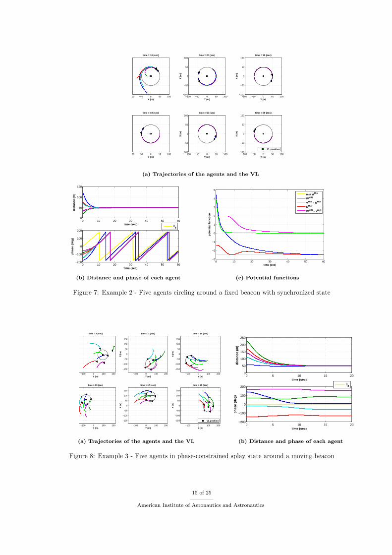
B. Example 2 : Synchronized circling around a fixed beacon with phase constraint

The second example uses the same settings as the first example, except that the desired phase configurationis a synchronized circling (M = 1). In addition, the phase constraint θd(t) = ω0t (rad) is imposed on theagent 1. Each agent motion is controlled by the controller (28) with the control gain Kθd

= Kθ. Figure7 shows trajectory profiles, relative distance and phase of each agent to the fixed beacon position, and thepotential functions UM,N (θ), V M,N (x) and WM,N (x) defined in (29). The difference WM,N (x)− V M,N (x)

13 of 25


corresponds to the phase reference tracking error of the agent 1. From the phase plot, one can see that aphase trajectory of the agent 1 (in blue) converges to its reference (in yellow). At the same time, the phasesof the other agents get to be synchronized and also converge to the reference. This convergence can beobserved clearly also in the plot of WM,N (x) which goes to its minimum.

C. Example 3 - Splay state around a moving beacon with phase constraint

The third example also uses the controller (28) with the phase constraint θd = 0 (rad) on the agent 1. Thedesired state in this example is a splay state (M = N) around a moving beacon with a radius r0 = 50 (m)and zero angular velocity ω0 = 0 (rad/sec). Let Xref , Xref and Xref be a reference position, velocity andacceleration for the beacon. Then, motion of the beacon is controlled to track this reference, independentlyfrom the agents’ motion, by using the following PD controller.

Xvl = −Kp(Xvl −Xref )−Kd(Xvl − Xref ) + Xref , Kp = 1, Kd = 3 (41)

In the simulation, the circle reference trajectory

Xref (t) = 100[

cos 0.4tsin 0.4t

](42)

is chosen. The initial position and velocity of the beacon are all zero. Figure 8(a) illustrates trajectoriesof the five agents and the moving beacon. Figure 8(b) shows profiles of distance and phase of each agentrelative to the beacon. The agents’ states are converging to the desired phase-constrained splay state.

D. Example 4 : Splay state around a center of mass with phase constraint

In the three examples presented above, the VL motion was completely known, and so are the relative distanceand phase dynamics of each agent. In this fourth example, the VL position and velocity are given by a centerof mass of the agents, i.e., by (19). Here we take over the same simulation settings as used in Example 3. Adesired VL acceleration ud is determined in the same manner as in (41) with the circle reference trajectory(42). It should be noted that the real VL acceleration Xvl does not necessary coincide with ud. Each agentmotion is controlled by the controller (36) with the phase constraint θ1 = θd = 0 (rad). The simulationresults are shown in Figure 9. Every agents’ states converge to the phase-constrained splay state, and inaddition, the motion of their center of mass (=virtual leader) follows its desired one. Figure 9(d) comparesthe VL desired and real accelerations (ud in red dashed vs. Xvl in blue solid), and shows that the differencebetween the two vanishes.

−100 −50 0 50 100−100

−50

0

50

100

Y (m)

time = 3 (sec)

−100 −50 0 50 100−100

−50

0

50

100

Y (m)

X (

m)

time = 7 (sec)

−100 −50 0 50 100−100

−50

0

50

100

Y (m)

X (

m)

time = 10 (sec)

−100 −50 0 50 100−100

−50

0

50

100

Y (m)

time = 13 (sec)

−100 −50 0 50 100−100

−50

0

50

100

Y (m)

X (

m)

time = 17 (sec)

−100 −50 0 50 100−100

−50

0

50

100

Y (m)

X (

m)

time = 20 (sec)

VL position 0 5 10 15 20−0.5

0

0.5

1

1.5

2

2.5

3

time (sec)

pote

ntia

l fun

ctio

n

min VM,N

VM,N

VM,N − UM,N

UM,N

(a) Trajectories of the agents and the VL (b) Potential functions

Figure 6: Example 1 - Five agents circling around a fixed beacon with splay state

14 of 25


−100 −50 0 50 100−100

−50

0

50

100

Y (m)

time = 10 (sec)

−100 −50 0 50 100−100

−50

0

50

100

Y (m)

X (

m)

time = 20 (sec)

−100 −50 0 50 100−100

−50

0

50

100

Y (m)

X (

m)

time = 30 (sec)

−100 −50 0 50 100−100

−50

0

50

100

Y (m)

time = 40 (sec)

−100 −50 0 50 100−100

−50

0

50

100

Y (m)

X (

m)

time = 50 (sec)

−100 −50 0 50 100−100

−50

0

50

100

Y (m)

X (

m)

time = 60 (sec)

VL position

(a) Trajectories of the agents and the VL

0 10 20 30 40 50 600

50

100

150

time (sec)

dis

tan

ce (

m)

0 10 20 30 40 50 60−200

−100

0

100

200

time (sec)

ph

ase

(deg

)

θd

0 10 20 30 40 50 60−3

−2

−1

0

1

2

3

4

5

time (sec)

pote

ntia

l fun

ctio

n

min WM,N

WM,N

VM,N − UM,N

UM,N

WM,N − VM,N

(b) Distance and phase of each agent (c) Potential functions

Figure 7: Example 2 - Five agents circling around a fixed beacon with synchronized state

−100 0 100 200Y (m)

time = 3 (sec)

−100 0 100 200

−150

−100

−50

0

50

100

150

Y (m)

X (

m)

time = 7 (sec)

−100 0 100 200

−150

−100

−50

0

50

100

150

Y (m)

X (

m)

time = 10 (sec)

−100 0 100 200Y (m)

time = 13 (sec)

−100 0 100 200

−150

−100

−50

0

50

100

150

Y (m)

X (

m)

time = 17 (sec)

−100 0 100 200

−150

−100

−50

0

50

100

150

Y (m)

X (

m)

time = 20 (sec)

VL position

0 5 10 15 200

50

100

150

200

250

time (sec)

dis

tan

ce (

m)

0 5 10 15 20−200

−100

0

100

200

time (sec)

ph

ase

(deg

)

θ

d

(a) Trajectories of the agents and the VL (b) Distance and phase of each agent

Figure 8: Example 3 - Five agents in phase-constrained splay state around a moving beacon

15 of 25


−100 0 100Y (m)

time = 7 (sec)

−100 0 100−150

−100

−50

0

50

100

150

Y (m)

X (

m)

time = 13 (sec)

−100 0 100−150

−100

−50

0

50

100

150

Y (m)

X (

m)

time = 20 (sec)

−100 0 100Y (m)

time = 27 (sec)

−100 0 100−150

−100

−50

0

50

100

150

Y (m)X

(m

)

time = 33 (sec)

−100 0 100−150

−100

−50

0

50

100

150

Y (m)

X (

m)

time = 40 (sec)

VL position


0 5 10 15 20 25 30 35 400

20

40

60

80

time (sec)

dis

tan

ce (

m)

0 5 10 15 20 25 30 35 40−200

−100

0

100

200

time (sec)

ph

ase

(deg

)

θd

0 5 10 15 20 25 30 35 40−0.5

0

0.5

1

1.5

2

2.5

3

3.5

4

time (sec)

pote

ntia

l fun

ctio

n

min WM,N

WM,N

VM,N − UM,N

UM,N

WM,N − VM,N


0 5 10 15 20 25 30 35 40−40

−20

0

20

40

Acc

eler

atio

n in

X(m

/sec

2 )

0 5 10 15 20 25 30 35 40−50

0

50

100

150

Acc

elra

tio

n in

Y

(m/s

ec2 )

time (sec)

VL accelerationu

d

(d) Desired and real VL accelerations

Figure 9: Example 4 - Five agents in phase-constrained splay state around their center of mass

16 of 25


E. Conclusion of Numerical Simulation

The proposed coordination controller has been tested through simulations with different configurations;

• different numbers of agents (N)

• the splay, synchronized and other (M, N)-pattern phase distributions

• with zero and non-zero angular velocities

• with or without phase constraint

• the VL position at a fixed/moving beacon and at a center of mass of the agents

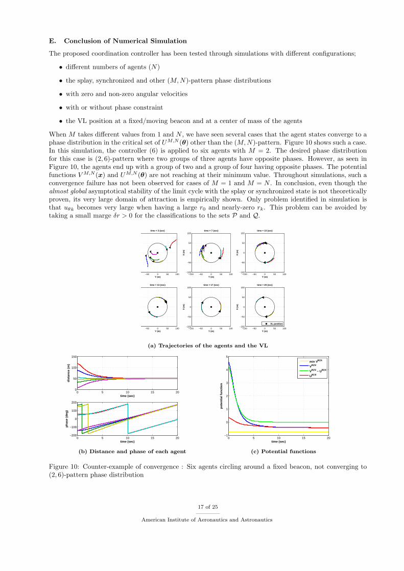
When M takes different values from 1 and N , we have seen several cases that the agent states converge to aphase distribution in the critical set of UM,N (θ) other than the (M,N)-pattern. Figure 10 shows such a case.In this simulation, the controller (6) is applied to six agents with M = 2. The desired phase distributionfor this case is (2, 6)-pattern where two groups of three agents have opposite phases. However, as seen inFigure 10, the agents end up with a group of two and a group of four having opposite phases. The potentialfunctions V M,N (x) and UM,N (θ) are not reaching at their minimum value. Throughout simulations, such aconvergence failure has not been observed for cases of M = 1 and M = N . In conclusion, even though thealmost global asymptotical stability of the limit cycle with the splay or synchronized state is not theoreticallyproven, its very large domain of attraction is empirically shown. Only problem identified in simulation isthat uθk becomes very large when having a large r0 and nearly-zero rk. This problem can be avoided bytaking a small marge δr > 0 for the classifications to the sets P and Q.

−50 0 50 100Y (m)

time = 3 (sec)

−100 −50 0 50 100−100

−50

0

50

100

Y (m)

X (

m)

time = 7 (sec)

−100 −50 0 50 100−100

−50

0

50

100

Y (m)

X (

m)

time = 10 (sec)

−50 0 50 100Y (m)

time = 13 (sec)

−100 −50 0 50 100−100

−50

0

50

100

Y (m)

X (

m)

time = 17 (sec)

−100 −50 0 50 100−100

−50

0

50

100

Y (m)

X (

m)

time = 20 (sec)

VL position


0 5 10 15 200

50

100

150

time (sec)

dis

tan

ce (

m)

0 5 10 15 20−200

−100

0

100

200

time (sec)

ph

ase

(deg

)

0 5 10 15 20−1

0

1

2

3

4

5

time (sec)

pote

ntia

l fun

ctio

n

min VM,N

VM,N

VM,N − UM,N

UM,N


Figure 10: Counter-example of convergence : Six agents circling around a fixed beacon, not converging to(2, 6)-pattern phase distribution

17 of 25


IV. Coordinated Flight of Multiple UAVs

In this section, the coordination controllers designed in Section II and validated in Section III is appliedto a mission of coordinated flight of multiple fixed-wing UAVs. The section first defines the entire missionscenario, then describes how to realize the onboard coordination control system architecture.

A. Mission Scenario

A global objective of the mission defined in this work is to make multiple UAVs track a flight plan, given bya sequence of waypoints (WP1 → WP2 → · · ·), in formation. The mission scenario consists of the followingfive phases.

• Phase 0 - Take-off : Each UAV is launched at any timing and follows the automatic take-off procedureuntil it reaches at a given fixed point (WP0). During this take-off phase, an UAV operates withoutany coordination with other UAVs.

• Phase 1 - Coordinated circling : Once a UAV reaches within a certain distance to the point WP0,it starts to make a circling motion around a fixed point (defined by WP0) with a constant speed andradius while making a splay state configuration with other UAVs who are already in Phase 1 (if any).It is achieved by applying the control law (6) with M = N where N is a number of UAVs in Phase 1and is re-counted at each communication update. The VL position is given by the fixed circle centerposition. This phase is considered as a waiting phase for all UAVs in the team to be launched in theair and to be ready for the formation flight.

• Phase 2 - Synchronized circling : After all UAVs in the team are in Phase 1, either an operatoror a decision-making algorithm can trigger a transition from the waiting phase to the formation phase.For a purpose of bringing all the UAVs close each other before making a formation, each UAV iscommanded to make a synchronized state configuration on the circle orbit. The transition from Phase1 to Phase 2 is realized simply by changing a value of M from N to 1 in the control law (6).

• Phase 3 - Circling in formation : When all the UAVs in the team assemble within a certaindistance on the circle, they start to make a formation by applying the control law (20), or (36) if onewish to impose a phase constraint, with M = N and ω0 = 0. r0 > 0 determines a formation distancebetween adjacent UAVs. In this phase, the VL position are defined by a mean of the UAV positionsas in (19). A control law for the VL motion (i.e., Xvl = ud) is designed independently from thecoordination control law so that it makes the same circling motion as in Phase 1 and 2.

• Phase 4 - Waypoint tracking in formation : A departing point is defined on the circle in functionof the circle position (WP0) and the first waypoint of the track (WP1). When the team of the UAVsreaches at this departing point, it quits the circle and departs for tracking a given sequence of thewaypoints (WP1 → WP2 → · · ·) while keeping the formation. The transition from Phase 3 to 4 isrealized by switching the control law for the VL motion from circling to waypoint tracking withoutany change in the coordination control law.

B. Decentralized Flight Control System Architecture

The coordination control system architecture is designed based on the one already developed onboard ourfixed-wing UAV platform for mono-use, which is illustrated in Figure 11(a). The system consists of the threecomponents; i) mission/waypoint management which deals with flight mode and waypoint changes, ii) guid-ance law which calculates speed, heading and altitude commands to achieve a given flight mode/waypoint,and iii) control law which calculates UAV actuator inputs from the guidance commands. This nominalcontrol system architecture is modified as shown in Figure 11(b) so that it allows coordination control withother UAVs. Note that a navigation filter which estimates the UAV current state from available onboardsensors and its feed-back loops to each component in the control system are omitted in those figures.

The coordination control law is incorporated in the system in a decentralized manner. That is, eachUAV receives states of every other UAVs in the team via communication, manages the coordination phase,and calculates the VL position and the coordination control commands by its own. As our coordinationcontroller is designed to compute the 2D acceleration command, it is converted to the horizontal velocity

18 of 25


(a) Mono-use (b) Coordination control

Figure 11: UAV Onborad Flight Control System Architecture

(speed+heading) command by integration. The altitude command is maintained constant at its desiredvalue. Besides the coordination control law, an anti-collision controller is added to assure UAV flight safety.It is very important to have this component especially for Phase 2, in which the UAVs try to get together.The anti-collision controller is designed based on an artificial potential method, and is activated only whenthe UAV gets closer to another UAV than a certain safety minimum distance. The guidance commands forcoordination and for anti-collision are combined into one, and then sent to the flight controller.

C. 6 DoF Flight Simulation

A 6 DoF flight simulator has been developed by ONERA/DCSD to mainly test performances of new guidanceand control laws and flight management systems before implementing them onboard our UAV platform fortheir in-flight validation. This simulator is realized as a C++ program and it includes;

• a simple flight dynamics model of a fixed-wing aircraft

• measurement models of onboard sensors (GPS, INS, barometer, etc.)

• flight safety and mission management system

• navigation filter for localization

• guidance law for available flight modes

• flight controller

• 3D OpenGL graphics and interactive user interface

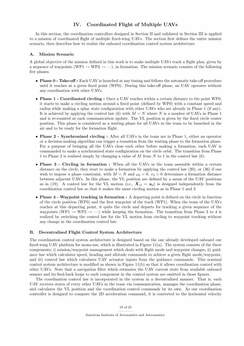
In this work, the simulator is first extended to simulate multiple UAVs at the same time. Then the coordina-tion control architecture shown in Figure 11(b) is implemented in it. The mission scenario for coordinationcontrol is pre-defined in the program, and transitions between the phases listed in Section IV.A are managedby a coordination phase management function. Figure 12 is a screen shot of the interface of this simulator,on which three fixed-wing UAVs are flying in formation. The interface accepts user’s input for flight modechanges, and a transition from Phase 1 to 2 is triggered by a user in the simulation.

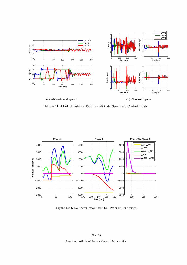
Figure 13 is a cutoff animation of the 6 DoF flight simulation for the entire mission scenario with threeUAVs. It shows the transitions of the coordination phases until the mission of waypoint tracking in formation(Phase 4) is achieved. In this simulation, a phase constraint of θj = 0 is imposed on one of the UAVs, wholocates the closest to the zero-phase position relative to the VL. Figure 14 presents the resulting altitude,speed, and control inputs (throttle, aileron, elevator and rudder) of each UAV. The speed plot shows thateach UAV regulates a speed within its limit to coordinate with the other UAVs during Phase 1 and Phase2. Figure 15 is a profile of the potential functions for each coordination phase. At each phase, the (M,N)-pattern potential function UM,N (θ) (in red) tends to converge to its global minimum (in yellow), whichmeans that the desired phase distribution is attained. In the formation flight (Phase 3 and 4), the formationtracking error (in green) and the reference phase tracking error (in magenta) are also converging to zero.

19 of 25


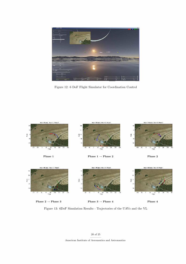
Figure 12: 6 DoF Flight Simulator for Coordination Control

Phase 1 Phase 1 → Phase 2 Phase 2

Phase 2 → Phase 3 Phase 3 → Phase 4 Phase 4

Figure 13: 6DoF Simulation Results - Trajectories of the UAVs and the VL

20 of 25


0 50 100 150 200 250 30020

25

30

35

40

Alt

itu

de

(m)

0 50 100 150 200 250 30030

40

50

60

70

time (sec)

Sp

eed

(km

/h)

UAV 1UAV 2UAV 3

0 100 200 3000

1

2

3

4

5

time (sec)

Th

rott

le

0 100 200 300−4

−2

0

2

4

time (sec)

Ele

vato

r (d

eg)

0 100 200 300−4

−2

0

2

4

time (sec)

Ru

dd

er (

deg

)

0 100 200 300−4

−2

0

2

4

time (sec)

Aile

ron

(d

eg)

UAV 1UAV 2UAV 3

(a) Altitude and speed (b) Control inputs

Figure 14: 6 DoF Simulation Results - Altitude, Speed and Control inputs

0 50 100−3000

−2000

−1000

0

1000

2000

3000

4000

Phase 1

Pot

entia

l Fun

ctio

ns

100 120 140 160 180−3000

−2000

−1000

0

1000

2000

3000

4000

Phase 2

time (sec)200 250 300

−3000

−2000

−1000

0

1000

2000

3000

4000

Phase 3 & Phase 4

min WM,N

WM,N

VM,N − UM,N

UM,N

WM,N − VM,N

Figure 15: 6 DoF Simulation Results - Potential Functions

21 of 25


D. UAV Platform and Onboard System

After the validation through 6 DoF flight simulation, the proposed coordination controller has been imple-mented and tested onboard the ONERA ReSSAC MOUSSE fixed-wing UAV platforms (Figure 4). Thisplatform is developed based on the R/C airplane Multiplex Twinstar II. Its specifications are summarizedin Table 2.

Table 2: Specifications

Empty weight 0.8 (kg)Take-off weight 2 (kg)Fuselage length 1 (m)Wingspan 1.4 (m)Motor electric×2Payload 0.5 (kg)Payload power supply 10 (W)Flight duration 40 (min)

Figure 16: Onboard Hardware

Figure 16 shows the onboard hardware system of the UAV. It is equipped with Xsens MTi inertialmeasurement units and µblox LEA-6H GPS. Two ARM7 micro processors (AT91SAM7) are embedded on theUAV; i) Processor CS (Switch Computer) takes charge of the radio command from a security pilot of the UAV,and ii) Processor CC (Control Computer) is dedicated to automatic flight navigation, guidance and control.The two processors are communicating each other via CAN bus datalink. The onboard hardware systemincludes a XBee wireless module which is used for communications with ground control station to downlinkthe flight state for data recording, and also with other UAVs to exchange the state data for coordinationcontrol. Figure 17 illustrates the onboard system architecture of the ReSSAC MOUSSE UAV. The softwareimplementation on the processors CS and CC is done in C++ program. The flight avionics system (onthe processor CC) consists of functions of flight management, mission management, communication, flightnavigation, guidance and control. All of these functions run in sequence with a periodic cycle of 50 (Hz). Inthis work, functions of the coordination phase management and of the coordination control are added in thissequence. They are programmed to perform only at 10 (Hz), once in every 5 iterations of the main-loop.The wireless communication function is also added in the sequence so that data exchange with other UAVsperforms at 8.5 (Hz), once in every 6 iterations.

The ground control station (GCS) for multi UAVs has been also developed for this work. The developedGCS program is executed in Linux system on a laptop computer, and it communicates with all the UAVsin operation via wireless connection at 8.5 (Hz). On its interface, trajectories of every UAVs are displayedin a main 3D scene window, and several important states (position, velocity, attitude, flight mode, batterylevel etc.) of each UAV are shown separately in other windows. All the state data received from UAVs arerecorded on the GCS. Although we are not currently using the uplink connection from the GCS to UAVs,there is a possibility to add it to send some commands and requests directly from the GCS without passingthrough radio command of the safety pilot.

E. Flight Experiment

Several flight experiments have been successfully conducted to perform the entire mission scenario definedin Section IV.A by three of our UAVs. Here presented the results obtained from the flight test on 22ndJuly, 2013. In this flight, three UAVs achieved a completely automatic flight in coordination from Phase0 (automatic take-off) to Phase 4 (waypoint tracking in formation) except the transition from Phase 1 toPhase 2 triggered by an operator on ground via radio command. The flight plan is given by four waypointpositions; WP0 defines the waiting zone (Phase 1-3), and WP1, WP2 and WP3 define the formation flightcircuit (Phase 4). During the waiting and transition phases (Phase 1-2), the UAVs are controlled to makea circling motion with a radius r0 = 60 (m) and a constant speed V0 = 55 (km/h), which gives an angularvelocity ω0 = 0.25 (rad/sec). For the formation flight phases (Phase 2-4), the formation distance between thetwo UAVs is set at 30 (m), and a phase constraint θj = 0 is imposed so that the UAVs aligns in North-South

22 of 25


Figure 17: Onboard System Architecture

directions. In the flight, three UAVs flew at three different altitudes, 50, 70 and 90 (m) for security reason.The coordination between the three is made only for their horizontal 2D positions.

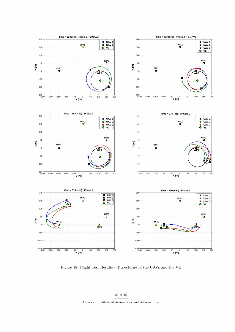
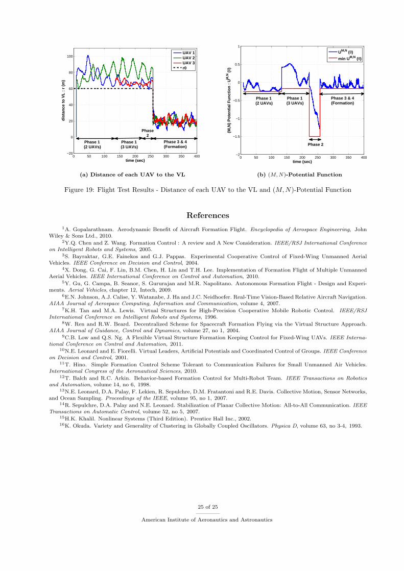
Figure 18 is a cut-off animation of the flight, which illustrates the transitions of the coordination phases.In each figure, positions of the UAVs, the VL, and the waypoints are shown. First, two UAVs made acoordinated circling, then the third one joined them on the circle (Phase 1). Triggered by an operator, thethree UAVs got close each other on the circle (Phase 2) before making a formation (Phase 3). Finally, theyleft for the mission of waypoint tracking while maintaining a formation (Phase 4). Figure 19(a) is a timeprofile of the distance of each UAV to the VL shown with its desired value r0. Figure 19(b) compares thereal and minimum value of the (M, N)-potential function UM,N (θ). For each phase of the coordination, thepotential function goes to its minimum. It means that the UAVs attains a desired phase distribution (splayor synchronized states). The commanded formation distance of 30 (m) is maintained with a precision of ±10(m). This precision can be still improved by synchronizing GPS measurements on every UAVs, by takinginto account a time delay of communication, by better regulating the control gains etc.

V. Conclusion

This paper proposed the decentralized coordination controller for multiple UAVs based on the virtualleader approach. The controller design uses a potential function on phase distribution, which attains itsglobal minimum at the desired splay/synchronized state. The first part of this paper provided a stabilityanalysis of the proposed coordination controller and its validation through numerical simulations. Then, thesecond half described the application of the controller to a fully autonomous formation flight of multipleUAVs. As a highlight of this paper, the flight experiment results of three UAVs formation were presented.In some flight tests, incoherent decisions between the UAVs were observed due to communication failure. Inorder to overcome this consensus issue of the decentralized system, a supervision function which monitors acoordination phase management state of every UAV should be added to the system.

Acknowledgments

The author appreciates Alexandre Amiez, Paul Chavent and Pierre Escalas in the ONERA ReSSAC UAVresearch team for their efforts to develop our UAV platforms and the onboard hardware/software systems.Without their work, the flight experiments would not have been conducted.

23 of 25


−250 −200 −150 −100 −50 0 50 100 150 200−150

−100

−50

0

50

100

150

200

Y (m)

X (

m)

time = 82 (sec) : Phase 1 − 2 UAVs

UAV 1UAV 2VL

WP1

WP0

WP3

WP2

−250 −200 −150 −100 −50 0 50 100 150 200−150

−100

−50

0

50

100

150

200

Y (m)

X (

m)

time = 193 (sec) : Phase 1 − 3 UAVs

UAV 1UAV 2UAV 3VL

WP0

WP1

WP2

WP3

−250 −200 −150 −100 −50 0 50 100 150 200−150

−100

−50

0

50

100

150

200

Y (m)

X (

m)

time = 254 (sec) : Phase 2

UAV 1UAV 2UAV 3VL

WP1

WP2

WP3

WP0

−250 −200 −150 −100 −50 0 50 100 150 200−150

−100

−50

0

50

100

150

200

Y (m)

X (

m)


UAV 1UAV 2UAV 3VL

WP1

WP2

WP3

WP0

−250 −200 −150 −100 −50 0 50 100 150 200−150

−100

−50

0

50

100

150

200

Y (m)

X (

m)


UAV 1UAV 2UAV 3VL

WP1

WP3

WP0

WP2

−250 −200 −150 −100 −50 0 50 100 150 200−150

−100

−50

0

50

100

150

200

Y (m)

X (

m)


UAV 1UAV 2UAV 3VL

WP1

WP2

WP3

WP0

Figure 18: Flight Test Results - Trajectories of the UAVs and the VL

24 of 25


0 50 100 150 200 250 300 350 400−20

0

20

40

60

80

100

time (sec)

dis

tan

ce t

o V

L :

r (

m)

UAV 1UAV 2UAV 3r0

Phase 1(2 UAVs)

Phase 1(3 UAVs)

Phase2

Phase 3 & 4(Formation)

0 50 100 150 200 250 300 350 400−2

−1.5

−1

−0.5

0

0.5

1

time (sec)

(M,N

) P

ote

nti

al F

un

ctio

n :

UM

,N (

θ)

UM,N (θ)

min UM,N (θ)

Phase 1(2 UAVs)

Phase 2

Phase 1(3 UAVs)

Phase 3 & 4(Formation)

(a) Distance of each UAV to the VL (b) (M, N)-Potential Function

Figure 19: Flight Test Results - Distance of each UAV to the VL and (M,N)-Potential Function

References

1A. Gopalarathnam. Aerodynamic Benefit of Aircraft Formation Flight. Encyclopedia of Aerospace Engineering, JohnWiley & Sons Ltd., 2010.

2Y.Q. Chen and Z. Wang. Formation Control : A review and A New Consideration. IEEE/RSJ International Conferenceon Intelligent Robots and Systems, 2005.

3S. Bayraktar, G.E. Fainekos and G.J. Pappas. Experimental Cooperative Control of Fixed-Wing Unmanned AerialVehicles. IEEE Conference on Decision and Control, 2004.

4X. Dong, G. Cai, F. Lin, B.M. Chen, H. Lin and T.H. Lee. Implementation of Formation Flight of Multiple UnmannedAerial Vehicles. IEEE International Conference on Control and Automation, 2010.

5Y. Gu, G. Campa, B. Seanor, S. Gururajan and M.R. Napolitano. Autonomous Formation Flight - Design and Experi-ments. Aerial Vehicles, chapter 12, Intech, 2009.

6E.N. Johnson, A.J. Calise, Y. Watanabe, J. Ha and J.C. Neidhoefer. Real-Time Vision-Based Relative Aircraft Navigation.AIAA Journal of Aerospace Computing, Information and Communication, volume 4, 2007.

7K.H. Tan and M.A. Lewis. Virtual Structures for High-Precision Cooperative Mobile Robotic Control. IEEE/RSJInternational Conference on Intelligent Robots and Systems, 1996.

8W. Ren and R.W. Beard. Decentralized Scheme for Spacecraft Formation Flying via the Virtual Structure Approach.AIAA Journal of Guidance, Control and Dynamics, volume 27, no 1, 2004.

9C.B. Low and Q.S. Ng. A Flexible Virtual Structure Formation Keeping Control for Fixed-Wing UAVs. IEEE Interna-tional Conference on Control and Automation, 2011.

10N.E. Leonard and E. Fiorelli. Virtual Leaders, Artificial Potentials and Coordinated Control of Groups. IEEE Conferenceon Decision and Control, 2001.

11T. Hino. Simple Formation Control Scheme Tolerant to Communication Failures for Small Unmanned Air Vehicles.International Congress of the Aeronautical Sciences, 2010.

12T. Balch and R.C. Arkin. Behavior-based Formation Control for Multi-Robot Team. IEEE Transactions on Roboticsand Automation, volume 14, no 6, 1998.

13N.E. Leonard, D.A. Palay, F. Lekien, R. Sepulchre, D.M. Fratantoni and R.E. Davis. Collective Motion, Sensor Networks,and Ocean Sampling. Proceedings of the IEEE, volume 95, no 1, 2007.

14R. Sepulchre, D.A. Palay and N.E. Leonard. Stabilization of Planar Collective Motion: All-to-All Communication. IEEETransactions on Automatic Control, volume 52, no 5, 2007.

15H.K. Khalil. Nonlinear Systems (Third Edition). Prentice Hall Inc., 2002.16K. Okuda. Variety and Generality of Clustering in Globally Coupled Oscillators. Physica D, volume 63, no 3-4, 1993.

25 of 25


coordinated control of multiple uavs: theory and flight

Documents