coordinate systems and georeference of norwegian …...map system. the projection origin is at a...

International Cartographic Association, Commission on Cartographic Heritage into the Digital Proceedings 12th ICA Conference Digital Approaches to Cartographic Heritage, Venice, 26-28 April 2017

Editor Evangelos Livieratos AUTH CartoGeoLab, 2017, ISSN 2459-3893

Aristotle University of Thessaloniki

[146] Laboratory of Cartography & Geographical Analysis

Gábor Timár1, Csilla Galambos2, Sidsel Kvarteig3, Előd Biszak4, Sándor Baranya5, Nils Rüther6

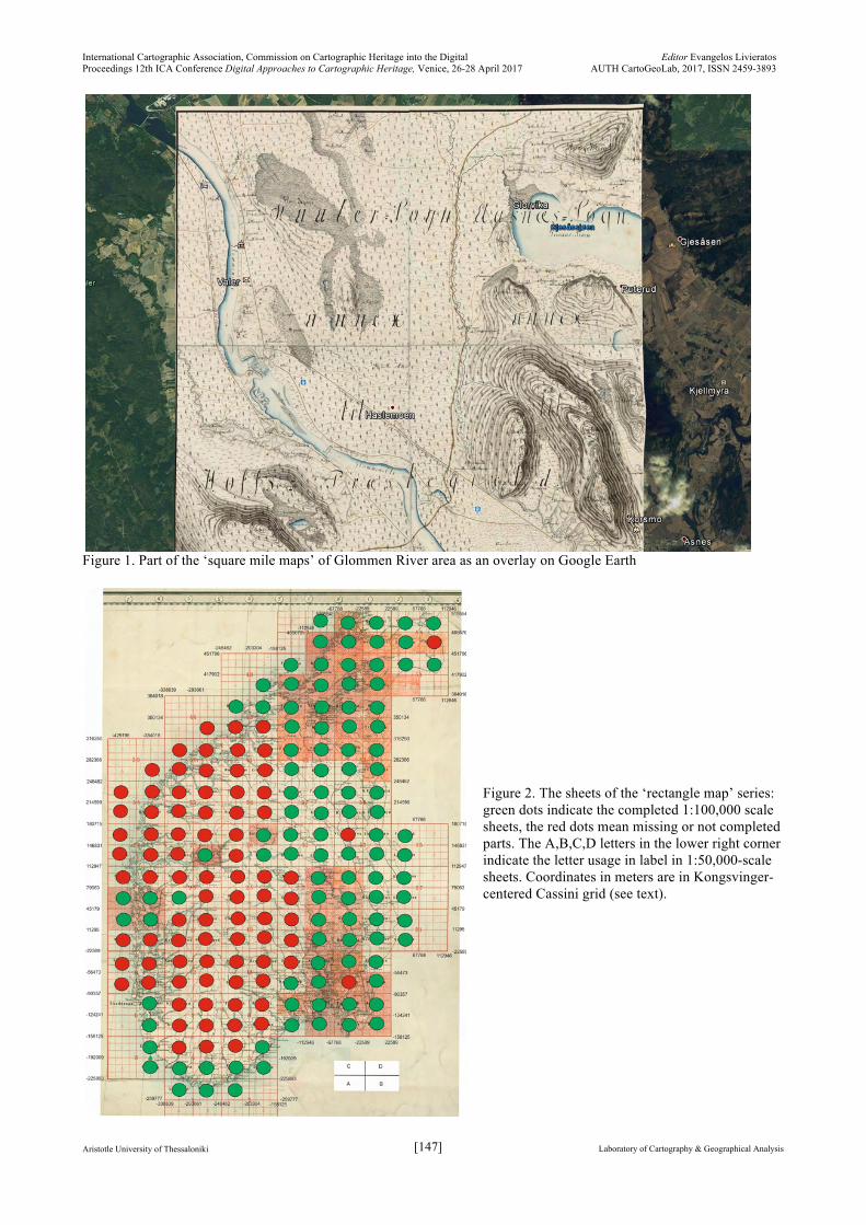
Coordinate systems and georeference of Norwegian historical topographic maps Key words: Norway, historical maps, topographic maps, 18th century, 19th century, georeference Summary The metadata of the Norwegian historical topographic maps are given, in order to make its georeference possible, using just their corners points as control points. The earliest systematic topographic map product is the square mile-maps (kvadratmil kart). They cover the southern leg of the Swedish border region of Norway as it was in the end of 18th century. The flagpole of the Kongsvinger fortress is the origin of the Cassini projection. The field extents of the sheets are 1*1 Old Norwegian mile; this is the origin of the name of the map system. The projection origin is at a sheet corner. The quality of the geodetic control is quite inhomogeneous. This map-series was followed by the rectangle-maps (rektangelkart). This system again covers only a part of Norway, mostly the area of the square mile maps plus Trondelag and the southern coast and the Bergen area. The scale is 1:100,000-survey time is the end of the 19th century and the first decade of the 20th one. The projection is still the Kongsvinger-centered Cassini type. The geodetic basis is much more precise than the one of its predecessor. With the relatively low scale, horizontal errors are practically eliminated. The terrain extent of the sheets is 4*3 Old Norwegian mile. The next and last studied series are the degree maps (Gradteigskart). In the beginning of the 20th century, the Norwegian mapping authority switched to application of the Gauss-Krüger (transverse Mercator) projection grids. The still missing, non-mapped parts, then almost the whole country was covered by the degree maps, in Gauss-Krüger zones. Corner GCPs can make the georeference and their geodetic coordinates (latitude and longitude) in the NGO datum, then re-project them to the respective Gauss-Krüger zone coordinates. Introduction The history of Norwegian topographic cartography starts with the mapping of the Swedish border area in the second half of the 18th century (Harsson, 2011). For the high-scale survey, an established geodetic network was needed. Its astronomical control was missing for a while. Astronomical expeditions to Norway to observe the 1761 and 1769 Venus transits helped to ‘hire’ experts to provide astronomical observations. A well-established triangulation network was constructed afterwards, making the area between the Glommen River and the Swedish border the best-surveyed part of Norway (for very interesting details, see the works of Pettersen, 2009; 2014). The later discussed square mile maps were compiled on the basis of this network (Fig. 1). A century later, that time already under Swedish rule, a new, 1:100,000-scale map product of Norway was decided to make. Not surprisingly, the ‘rectangle maps’ series was started to compile again in this, better surveyed part of the country, later completed with other economically important parts, e.g. the southern coasts and the largest western ports (Fig. 2). However the resulted maps were republished in corrected form but in the same sheet system and projection till mid-1900s, the international trend appeared also in Norway and around the independence time, the country decided to apply the conformal transverse Mercator projection of Gauss. The last ‘historical’ map product before the present-day maps were the degree maps, already in this projection, covering first the so far not mapped area, then majority (but not the all) of the coverage of the rectangle maps. Parameters needed for geo-reference of all above historical maps are estimated, and based on them, the geo-referenced mosaic of rectangle maps have been published in MAPIRE.

1 Dept. of Geophysics and Space Science, Eötvös University, Budapest 2 Dept. of Geological and Geophysical Collections, Geological and Geophysical Institute of Hungary, Budapest 3 Kartverket – Norwegian Map Authority, Hønefoss 4 Arcanum Database Ltd., Budapest 5 Dept. of Hydraulic and Water Resources Engineering, Budapest University of Technology and Economics 6 Dept. of Civil and Environmental Engineering, Norwegian University of Science and Engineering, Trondheim





Figure 1. Part of the ‘square mile maps’ of Glommen River area as an overlay on Google Earth

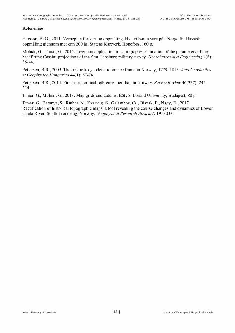
Figure 2. The sheets of the ‘rectangle map’ series: green dots indicate the completed 1:100,000 scale sheets, the red dots mean missing or not completed parts. The A,B,C,D letters in the lower right corner indicate the letter usage in label in 1:50,000-scale sheets. Coordinates in meters are in Kongsvinger-centered Cassini grid (see text).





The georeferencing process and its result During the georeferencing process we define ground control points (GCPs) in the scanned map. We give their position in the scanned image, as well as their map coordinates. The minimum number of the GCPs is three, however if we’d like to see the transformation errors, we shall have at least a fourth one, too. The goereferencing software estimates the parameters of the image-to-map linear transformation. The error represents the average distance in pixel units between the computed and given map coordinates at all GCPs. In case of modern maps, we can accept a fit with better than 2-3 pixels of error, however in case of a historical map this error margin can go up to 10-15 pixels. Higher error values indicate any theoretical error (most probably the selection of wrong projection) or a misplaced GCP, with given erroneous coordinates. Sometimes we use map products, consisting of many sheets in a uniform system, covering a whole country or region. Georeferencing such a map system we avoid to use real terrain objects as GCPs, if possible. GCPs are selected at the corners of the map frame or at the crossing or crosshairs of coordinate lines or latitude/longitude lines. The borders of a unique sheet of such a system are usually coordinate lines in some system. If the shape of the sheet is rectangle, then they are north-south and east-west grid lines in the original projection of the sheet (square mile maps, kvadratmil kart and rectangle maps, rektangelkart). If the shape of the sheet is a degree trapezoid then the frame borders run on latitude and longitude lines (degree maps, gradteigskart). While georeferencing a rectangle-shaped sheet, we choose practically the four corner points of the sheet. In this case, beyond the definition of the coordinate system, we shall know the location of the sheets in this very system. This location if defined by

• the location of the projection origin in the system of the sheets (the origin is in which sheet at what position, or it is in a corner of which sheets)

• the terrain extents of the sheets. If the sheet labels are given systematically, with consequent row and column numbers, the coordinates of the corners can be easily given by simple addition and multiplication based on the above information. In other cases, an overview map is needed or to be created, to give the location of the individual sheets in the projection plane, thus defining the coordinates of its corners. We shall be well aware that most of the historical maps are made before the introduction of the metric system. In Hungary, the basis of the map coordinates was the Viennese fathom, while in Norway; it was the alen-based Old Norwegian mile (gamle norsk mil). If only the latitude and longitude lines are given in the map, the georeferencing process needs an extra step. In the first step, the corner points or latitude/longitude crossings are defined as GCPs with their ellipsoidal latitudes and longitudes. Not to be surprised, if at first it leads to relatively high errors as the map is not in this coordinate system (the latitude and longitude lines form no parallel and perpendicular line sets). In the second step, we re-compute these figures into the genuine projection of the map, using our GIS software applied for the georeferenced. The errors shall be pretty low after this last step. The result of the georeference is a map with a coordinate system, which is correctly defined. This enables us to draw the scanned map image in all known projection system. For example, it can be shown as a layer in OpenStreetMap database. This way, the old, mapped terrain status can be compared to the modern one, and e.g. precise GPS coordinates can be tagged for the information items of the old map. Moreover, if more historical maps cover the same area from different time, they can be also fit to each other, providing a kind of ‘time machine’ in our application. The historical topographic maps of Norway Square mile maps (kvadratmil kart) Their scale is around 1:10,000. They cover the southern leg (up to the southern border of Trondelag) of the Swedish border region of Norway in its status in the end of 18th century (1779-1812; Pettersen, 2014). The Kongsvinger fortress flagpole is the origin in the Cassini projection (Pettersen, 2009). The field extents of the sheets are 1*1 Old Norwegian mile (gamle norsk mil); this is the origin of the name





of the map system. Corner GCPs based on an overview map and counting the corners northern and eastern distance from the projection origin in miles can provide Georeference. The quality of the geodetic control is quite inhomogeneous: in the middle parts and around the modern city of Oslo it is quite precise (Fig. 3). However, in the astronomically less-controlled southern parts, the errors can be as high as 2-3 kilometers. For better results in the best-controlled part of the maps, a 160-meter northward shift has to be applied on the NGO datum definition, which is pretty suitable for the geo-reference of even for these old maps.

Figure 3. Kristiania (now Oslo) in the ‘square map’ sheet, as on overlay in Google Earth, after the 160-meter northward correction (see text).

Fig. 4. Lower part of Gaula River in the 1:50,000-scale version of the ‘rectangle maps’, from 1868, in Google Earth background.

Rectangle maps (Rektangelkart) This system again covers only a part of Norway, mostly the area of the square mil maps plus Trondelag and the economically important southern part/coast of the country and the area of Bergen (Harsson, 2011. The scale is 1:100,000-survey time is the end of the 19th century and the first decade of the 20th one. The projection is still the Kongsvinger-centered Cassini type. The geodetic basis is much more precise than the one of its predecessor. With the relatively low scale, horizontal errors are practically eliminated. The terrain extents of the sheets are 4*3 Old Norwegian mile. The projection origin is 2 miles to east and 1 mile to south of the northwestern corner of the containing sheet. Georeference is made based on projection coordinates of the corner GCPs (see coordinate figures in Fig. 2). Larger scale working version of this map product (e.g. in 1:50,000 scale; Fig. 5) was completed for some parts of the mapped area. Degree maps (Gradteigskart) In the beginning of the 20th century, the Norwegian mapping authority switched to application of the Gauss-Krüger (transverse Mercator) projection grids. Production of the rectangle maps has been stopped. The still missing, non-mapped parts of the country were covered by the 1:100,000 scale degree map system in Gauss-Krüger zones. Later it was extended to the most parts covered earlier by the rectangular maps, providing an almost full cover of Norway. The terrain extents of the sheets are not uniform: it varies with the geographic latitude. Corner GCPs can make the georeferenced and their geodetic coordinates (latitude and longitude) in the NGO datum, then re-project them to the respective Gauss-Krüger zone coordinates. Georeferenced product in MAPIRE At the time of this report and presentation, the ‘rectangle maps’ (Rektangelkart) series has been published in the MAPIRE as a georeferenced mosaic, showing the physical picture of eastern Norway and some western coast area in the time of the change of 19th and 20th centuries (Figs. 5 & 6). The





results are applied in virtual reconstruction of the environment prior to the dam buildings as well as the original dynamics of the rivers (Timár et al., 2017), however the possible fields of the applications has a much wider range in geography and economy.

Fig. 5. The Norwegian rectangle map series in the MAPIRE

Fig. 6. Georeferenced mosaic of Trondheim area in the MAPIRE Acknowledgements Map samples are published by the Kartverket and used here with their permission. The research was carried out in the frame of EEA/156/M4-0002 project.





References Harsson, B. G., 2011. Verneplan for kart og oppmåling. Hva vi bør ta vare på I Norge fra klassisk oppmåling gjennom mer enn 200 år. Statens Kartverk, Hønefoss, 160 p.

Molnár, G., Timár, G., 2015. Inversion application in cartography: estimation of the parameters of the best fitting Cassini-projections of the first Habsburg military survey. Geosciences and Engineering 4(6): 36-44.

Pettersen, B.R., 2009. The first astro-geodetic reference frame in Norway, 1779–1815. Acta Geodaetica et Geophysica Hungarica 44(1): 67-78.

Pettersen, B.R., 2014. First astronomical reference meridian in Norway. Survey Review 46(337): 245-254.

Timár, G., Molnár, G., 2013. Map grids and datums. Eötvös Loránd University, Budapest, 88 p.

Timár, G., Baranya, S., Rüther, N., Kvarteig, S., Galambos, Cs., Biszak, E., Nagy, D., 2017. Rectification of historical topographic maps: a tool revealing the course changes and dynamics of Lower Gaula River, South Trondelag, Norway. Geophysical Research Abstracts 19: 8033.

coordinate systems and georeference of norwegian …...map system. the projection origin is at a...

Documents