Acta Geod Geophys (2014) 49:37–55DOI 10.1007/s40328-013-0038-0

Coordinate estimation accuracy of static precise pointpositioning using on-line PPP service, a case study

K. Dawidowicz · G. Krzan

Received: 3 September 2013 / Accepted: 14 December 2013 / Published online: 9 January 2014© Akadémiai Kiadó, Budapest, Hungary 2014

Abstract Precise Point Positioning (PPP) is a combination of the original absolute posi-tioning concept and differential positioning techniques. In PPP we use observation datafrom a single receiver and additional information of GNSS biases and errors derived frompermanent networks. Since PPP was developed based only on GPS observations, the accu-racy, availability and reliability of positioning is quite dependent on the number of visiblesatellites. One possible way to increase the availability of satellites is to integrate GPS andGLONASS observations. Nowadays such integration in PPP is available.

The PPP technique has an essential advantage over differential methods. The user needsonly a single receiver to obtain accurate position. Unfortunately, current commercial soft-ware does not provide processing of measurements taken using the PPP technique. Thisrequires using scientific software or one of several on-line PPP services.

This paper presents an analysis of the position determination accuracy in PPP mode. Weprocessed 6 consecutive days of GPS+GLONASS data using the on-line PPP-CSRS serviceto determine how the accuracy of derived three-dimensional positional coordinates dependson the length of the observing session, the characteristics of horizon visibility on points andthe observations used in post-processing (GPS or GPS+GLONAS, L1 or L1+L2).

The PPP-CSRS results show that horizontal accuracies of about 5 cm and vertical accu-racies of 10 cm are achievable provided 0.5 hours of open sky, low multipath dual frequencyGPS-only data. The accuracies clearly decrease for points measured under conditions oflimited availability of satellites. Unexpectedly, adding GLONASS observations generallydoes not improve the results in this case.

Keywords PPP · CSRS · GPS · GLONASS · Static measurements accuracy

1 Introduction

The Global Navigation Satellite System (GNSS) generally provides two techniques: abso-lute or differential (relative) positioning. Classical absolute positioning does not provide

K. Dawidowicz (B) · G. KrzanUniversity of Warmia and Mazury, Oczapowskiego 1, 10-719 Olsztyn, Polande-mail: karol.dawidowicz@uwm.edu.pl

38 Acta Geod Geophys (2014) 49:37–55

the accuracy required for surveying tasks. Highly accurate results can be obtained usingDifferential GNSS (DGNSS). At least two simultaneously operating receivers are requiredfor differential positioning (Hofmann-Wellenhof et al. 2008; Parkinson and Spilker 1996;Seeber 2003).

Currently, in many countries differential techniques are also supported by well-developedreference station infrastructure (Dawidowicz 2013; Snay and Soler 2008; Nejat and Kiamehr2013). Due to the high costs of establishing and maintaining a network of permanent sta-tions, as well as the fact that highly precise satellite orbits, clock corrections or atmosphericproducts are made available by such centers as the International GNSS Service (IGS), theCenter for Orbit Determination for Europe (CODE) or the Jet Propulsion Laboratory (JPL),many research programs studying the Precise Point Positioning (PPP) technique have beenundertaken in recent years (Alcay et al. 2012a, 2012b; Rizos et al. 2012).

PPP, which is a relatively new category is a combination of the absolute positioning con-cept and differential positioning techniques. It is based on the processing of observationsfrom a single GNSS receiver and employs a number of corrections (Kouba and Héroux 2001;Rizos et al. 2012; Zumberge et al. 1997). In PPP, observations from a base station are notused and the absence of differentiation of observations necessitates using precise satelliteorbits and clock corrections in the post-processing as well as modeling iono- and tropo-spheric refractions, solid earth and ocean tides, antenna phase-center offsets and variations,carrier-phase wind-up, relativistic effects, etc. (Rizos et al. 2012). To determine these fac-tors, continuous satellite observations or laboratory tests are needed.

The mathematical model of static or kinematic PPP is widely described in the literature,i.e.: Choy 2011; Cai and Gao 2007; Elsobeiey and El-Rabbany 2011; Gao et al. 2005. Theobservational equations for code (1) and phase (2) measurements are:

P = ρ + cdtr + cdtb + �trp + �ion + ε (1)

Φ = ρ + cdtr + cdtb + λN + �trp − �ion + ε (2)

where P is the pseudo-range between satellite and receiver, Φ is the difference betweenthe phases of signals in the moment t , ρ is the geometric distance between satellite andreceiver, c is the speed of light, dtr is the difference between time of signal transmissionand signal reception, dtb is the difference between satellite and receiver clock biases, �trp

is the tropospheric delay, �ion is the ionospheric delay, λ is the wavelength, N is the phaseambiguity and ε means other errors.

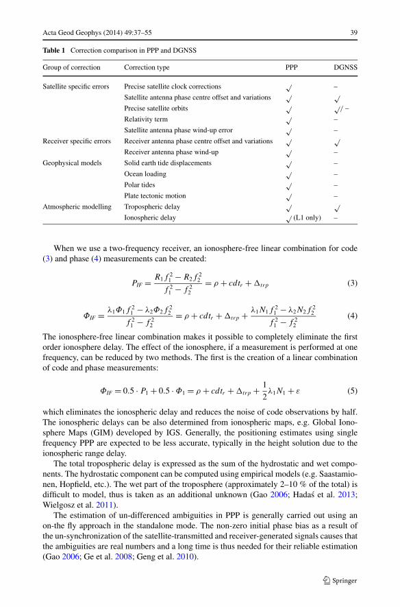
In PPP, the symbol ε includes many more bases and errors than in DGNSS. The completecomparison of the corrections that need to be applied in PPP and DGNSS is presented inTable 1 (Rizos et al. 2012).

Orbital errors in the PPP are reduced using precise orbits.Because the GNSS satellite clocks are difficult to model, appropriate corrections have to

be applied. This data can be obtained, for example, from the IGS (Gao and Kongzhe 2004;Kouba and Héroux 2001).

The most common method to eliminate first-order, ionospheric error is to use a combi-nation of dual frequency observations (Cai and Gao 2007; Elsobeiey and El-Rabbany 2011;Moreno et al. 2011).

Single frequency PPP is one of the most challenging research topics. The effect ofthe ionosphere remains the dominant error source for GNSS data processing on a singlefrequency. The difference between single frequency and dual frequency processing is themethod in which the ionospheric delay can be mitigated.

Acta Geod Geophys (2014) 49:37–55 39

Table 1 Correction comparison in PPP and DGNSS

Group of correction Correction type PPP DGNSS

Satellite specific errors Precise satellite clock corrections √ –

Satellite antenna phase centre offset and variations √ √Precise satellite orbits √ √

/ –

Relativity term √ –

Satellite antenna phase wind-up error √ –

Receiver specific errors Receiver antenna phase centre offset and variations √ √Receiver antenna phase wind-up √ –

Geophysical models Solid earth tide displacements √ –

Ocean loading √ –

Polar tides √ –

Plate tectonic motion √ –

Atmospheric modelling Tropospheric delay √ √Ionospheric delay √ (L1 only) –

When we use a two-frequency receiver, an ionosphere-free linear combination for code(3) and phase (4) measurements can be created:

PIF = R1f21 − R2f

22

f 21 − f 2

2

= ρ + cdtr + �trp (3)

ΦIF = λ1Φ1f2

1 − λ2Φ2f2

2

f 21 − f 2

2

= ρ + cdtr + �trp + λ1N1f21 − λ2N2f

22

f 21 − f 2

2

(4)

The ionosphere-free linear combination makes it possible to completely eliminate the firstorder ionosphere delay. The effect of the ionosphere, if a measurement is performed at onefrequency, can be reduced by two methods. The first is the creation of a linear combinationof code and phase measurements:

ΦIF = 0.5 · P1 + 0.5 · Φ1 = ρ + cdtr + �trp + 1

2λ1N1 + ε (5)

which eliminates the ionospheric delay and reduces the noise of code observations by half.The ionospheric delays can be also determined from ionospheric maps, e.g. Global Iono-sphere Maps (GIM) developed by IGS. Generally, the positioning estimates using singlefrequency PPP are expected to be less accurate, typically in the height solution due to theionospheric range delay.

The total tropospheric delay is expressed as the sum of the hydrostatic and wet compo-nents. The hydrostatic component can be computed using empirical models (e.g. Saastamio-nen, Hopfield, etc.). The wet part of the troposphere (approximately 2–10 % of the total) isdifficult to model, thus is taken as an additional unknown (Gao 2006; Hadas et al. 2013;Wielgosz et al. 2011).

The estimation of un-differenced ambiguities in PPP is generally carried out using anon-the fly approach in the standalone mode. The non-zero initial phase bias as a result ofthe un-synchronization of the satellite-transmitted and receiver-generated signals causes thatthe ambiguities are real numbers and a long time is thus needed for their reliable estimation(Gao 2006; Ge et al. 2008; Geng et al. 2010).

40 Acta Geod Geophys (2014) 49:37–55

Additional biases and errors that have to be estimated in the PPP include:

– the Sagnac effect caused by the Earth’s rotation during the transmission of the signal,– phase wind up, due to the relative motion and rotation of the satellite and receiver,– relativity error, which is a function of the satellite motion and the Earth’s gravity,– inter-frequency bias, appears when using a single frequency.

PPP was developed based on only GPS observations. The accuracy, availability and re-liability of positioning are, however, quite dependent on the number of visible satellites.In environments of urban canyons, nearby buildings and trees, the number of visible GPSsatellites is often insufficient for accurate position determination. Even if there are sufficientGPS satellites available, the PPP accuracy and reliability may still be insufficient due topoor satellite geometry. One possible way to increase the availability, reliability and accu-racy is to integrate GPS and GLONASS observations. Nowadays, such integration in PPP isavailable.

Since the International GLONASS Experiment (IGEX-98) and the GLONASS ServicePilot Project (IGLOS) conducted in 1998 and 2000, respectively (Weber et al. 2005), theprecise GLONASS orbit and clock data have become available. Currently, four IGS anal-ysis centers are routinely providing GLONASS precise orbit products with an accuracylevel of about 10–15 cm. They are the Center of Orbit Determination in Europe (CODE),Information—Analytical Center (IAC), European Space Operations Center (ESOC) andBundesamt für Kartographie und Geodäsie (BKG). Two data analysis centers (IAC andESOC) provide post-mission GLONASS satellite clock data with an accuracy level of about1.5 ns (Oleynik et al. 2006; Rizos et al. 2012). This provides opportunities to use GLONASSobservations to improve precise point positioning accuracy. Although the GPS/GLONASSobservations processing creates some additional difficulties, e.g. a system time differenceunknown parameter should be introduced for observation processing. A receiver clock errorcan be described as:

dt = t − tsys (6)

where tsys denotes either GPS system time (tGPS) for GPS observations or GLONASS sys-tem time (tGLONASS) for GLONASS observations. Since the receiver clock error is related toa system time, the combined GPS and GLONASS processing includes two receiver clockoffset unknown parameters, one for the receiver clock offset with respect to the GPS timeand one for the receiver clock offset with respect to the GLONASS time. Additionally, inGPS/GLONASS observations processing, ambiguity parameters equal to the number of ob-served GPS and GLONASS satellites. The problem of combined GPS/GLONASS process-ing was described in detail, for example, in: Alcay et al. (2012a, 2012b), Bruyninx (2007),Dodson et al. (1999), Cai and Gao (2007).

The main focus of this study was an investigation on the coordinates estimation accuracyof static Precise Point Positioning using on-line PPP services. Seven days GNSS obser-vations were made at 3 points with different characteristics of horizon visibility. Recentlyseveral PPP software packages have been developed by different research centers and it hasbeen proven that centimeter-level point positioning is achievable in post-processed, staticdual-frequency mode (e.g. Choy 2011; Gao and Kongzhe 2004; Zumberge et al. 1997).It was found (Ebner and Featherstone 2008) that post-processed PPP offers very compa-rable accuracies to the DGNSS technique. Comparing free PPP post-processing servicesresults from 1-hour and longer observations with coordinates derived from a Bernese soft-ware (Grinter and Janssen 2012) it was proven that we can obtain solutions not significantlydiffering.

Acta Geod Geophys (2014) 49:37–55 41

In our study, we shortened the minimum time of observation to 30 min. Shortening theobservation time hinders the resolution of integer ambiguities and also provides less data forestimating the parameters associated with tropospheric refraction. Additionally, we analyzeaccuracy depending on satellites visibility on points—two receivers collected observationsunder conditions of limited satellite availability. Comparison also include the analysis of re-sult differences between GPS only and combined GPS/GLONASS observations processingas well as the analysis of the position determination accuracy using one and two measure-ment frequencies.

For processing, the Canadian Spatial Reference System—Precise Point Positioning(CSRS-PPP) service was chosen.

2 Research area

Web-based PPP services are a practical alternative for software used for the post-processingof satellite observations by a user. Additionally, since current commercial software pack-ages do not provide the processing of measurements done using PPP, it is necessary to usescientific software or one of several online services. These services differ in processing al-gorithms, the origin of the error models used as well as the form of making the processingresults available. The most popular PPP services are briefly described below.

APPS provided by JPL California Institute of Technology (https://apps.gdgps.net/),which uses models of orbits and clock errors from its own system. The service allows usersto perform the post-processing of static and kinematic observations at two frequencies; ob-servations from the GLONASS system are not used in post-processing.

CSRS-PPP provided by Natural Resources Canada (http://www.geod.nrcan.gc.ca/),which uses models of orbits and clock errors developed by the IGS services. CSRS-PPPallows post-processing static and kinematic observations and uses observations from theGPS and GLONASS systems.

Examples of other systems include: GAPS (http://gaps.gge.unb.ca/indexv2.php),AUSPOS—Online GPS Processing Service (http://ga.gov.au/bin/gps.pl), Trimble Center-Point RTX (http://trimblertx.com/).

For our analysis the Canadian Spatial Reference System—Precise Point Positioning(CSRS-PPP) service was chosen. We chose the CSRS-PPP service due to the fact that ob-servations files can be uploaded from the website or through the PPP Direct software. Addi-tionally CSRS-PPP is one of the few services which allows L1-only data processing. Afterpost-processing, the user receives not only the coordinates and their sigmas in the ITRF2008or NAD83 system, but also diagrams of the visibility of satellites, the temporal convergenceof coordinates, the estimated tropospheric delay and clock offset as well as detailed obser-vational data from each measurement epoch, etc. Additionally, as was mentioned earlier,CSRS-PPP allows post-processing observations from the GPS and GLONASS system.

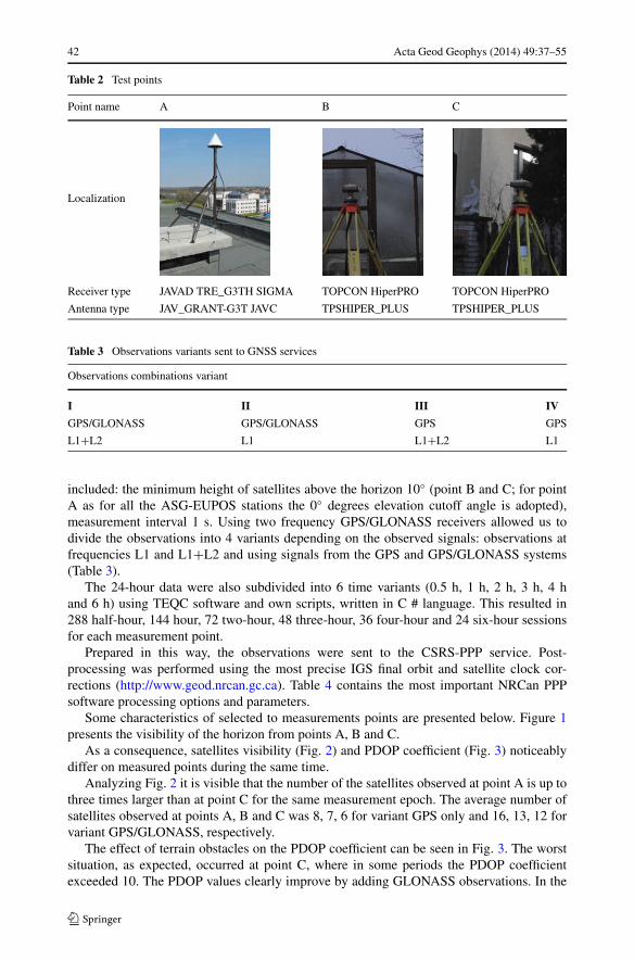
Seven days of static measurements from three GNSS stations are used in this reportto evaluate the accuracy of position determination in PPP-CSRS services. As a point A,the ASG-EUPOS reference station KROL in Olsztyn was adopted, assuming that this isthe point with optimal observing conditions without any obstructions. Points B and C aremarked in an urban area, where trees or buildings limit the number of observed satellitesand increase the risk of multipath (Table 2).

Measurements were carried out for seven days (from 20 to 26 November 2012) usingGPS/GLONASS receivers. The sessions started and ended at 17:00, thus we finally obtainedsix 24-hour measurement data. The GNSS parameters we adopted for measurement sessions

42 Acta Geod Geophys (2014) 49:37–55

Table 2 Test points

Point name A B C

Localization

Receiver type JAVAD TRE_G3TH SIGMA TOPCON HiperPRO TOPCON HiperPRO

Antenna type JAV_GRANT-G3T JAVC TPSHIPER_PLUS TPSHIPER_PLUS

Table 3 Observations variants sent to GNSS services

Observations combinations variant

I II III IV

GPS/GLONASS GPS/GLONASS GPS GPS

L1+L2 L1 L1+L2 L1

included: the minimum height of satellites above the horizon 10◦ (point B and C; for pointA as for all the ASG-EUPOS stations the 0◦ degrees elevation cutoff angle is adopted),measurement interval 1 s. Using two frequency GPS/GLONASS receivers allowed us todivide the observations into 4 variants depending on the observed signals: observations atfrequencies L1 and L1+L2 and using signals from the GPS and GPS/GLONASS systems(Table 3).

The 24-hour data were also subdivided into 6 time variants (0.5 h, 1 h, 2 h, 3 h, 4 hand 6 h) using TEQC software and own scripts, written in C # language. This resulted in288 half-hour, 144 hour, 72 two-hour, 48 three-hour, 36 four-hour and 24 six-hour sessionsfor each measurement point.

Prepared in this way, the observations were sent to the CSRS-PPP service. Post-processing was performed using the most precise IGS final orbit and satellite clock cor-rections (http://www.geod.nrcan.gc.ca). Table 4 contains the most important NRCan PPPsoftware processing options and parameters.

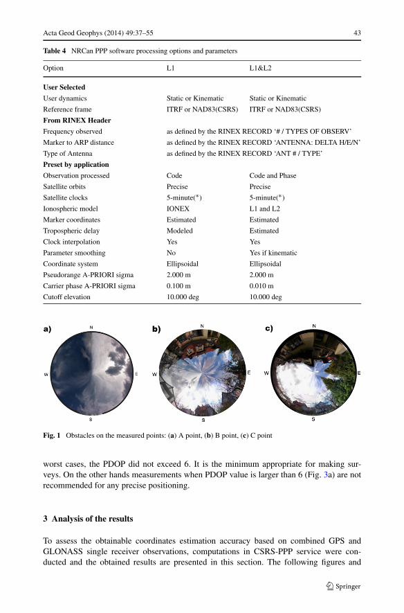
Some characteristics of selected to measurements points are presented below. Figure 1presents the visibility of the horizon from points A, B and C.

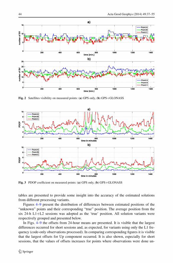
As a consequence, satellites visibility (Fig. 2) and PDOP coefficient (Fig. 3) noticeablydiffer on measured points during the same time.

Analyzing Fig. 2 it is visible that the number of the satellites observed at point A is up tothree times larger than at point C for the same measurement epoch. The average number ofsatellites observed at points A, B and C was 8, 7, 6 for variant GPS only and 16, 13, 12 forvariant GPS/GLONASS, respectively.

The effect of terrain obstacles on the PDOP coefficient can be seen in Fig. 3. The worstsituation, as expected, occurred at point C, where in some periods the PDOP coefficientexceeded 10. The PDOP values clearly improve by adding GLONASS observations. In the

Acta Geod Geophys (2014) 49:37–55 43

Table 4 NRCan PPP software processing options and parameters

Option L1 L1&L2

User Selected

User dynamics Static or Kinematic Static or Kinematic

Reference frame ITRF or NAD83(CSRS) ITRF or NAD83(CSRS)

From RINEX Header

Frequency observed as defined by the RINEX RECORD ‘# / TYPES OF OBSERV’

Marker to ARP distance as defined by the RINEX RECORD ‘ANTENNA: DELTA H/E/N’

Type of Antenna as defined by the RINEX RECORD ‘ANT # / TYPE’

Preset by application

Observation processed Code Code and Phase

Satellite orbits Precise Precise

Satellite clocks 5-minute(∗) 5-minute(∗)

Ionospheric model IONEX L1 and L2

Marker coordinates Estimated Estimated

Tropospheric delay Modeled Estimated

Clock interpolation Yes Yes

Parameter smoothing No Yes if kinematic

Coordinate system Ellipsoidal Ellipsoidal

Pseudorange A-PRIORI sigma 2.000 m 2.000 m

Carrier phase A-PRIORI sigma 0.100 m 0.010 m

Cutoff elevation 10.000 deg 10.000 deg

Fig. 1 Obstacles on the measured points: (a) A point, (b) B point, (c) C point

worst cases, the PDOP did not exceed 6. It is the minimum appropriate for making sur-veys. On the other hands measurements when PDOP value is larger than 6 (Fig. 3a) are notrecommended for any precise positioning.

3 Analysis of the results

To assess the obtainable coordinates estimation accuracy based on combined GPS andGLONASS single receiver observations, computations in CSRS-PPP service were con-ducted and the obtained results are presented in this section. The following figures and

44 Acta Geod Geophys (2014) 49:37–55

Fig. 2 Satellites visibility on measured points: (a) GPS only, (b) GPS+GLONASS

Fig. 3 PDOP coefficient on measured points: (a) GPS only, (b) GPS+GLONASS

tables are presented to provide some insight into the accuracy of the estimated solutionsfrom different processing variants.

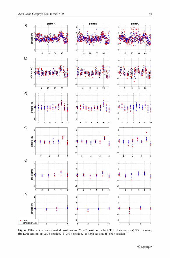
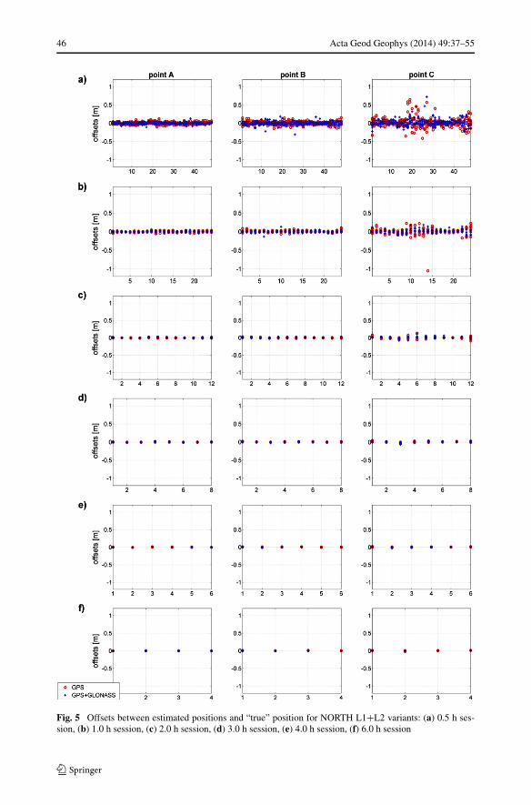
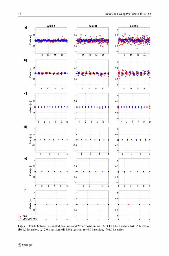
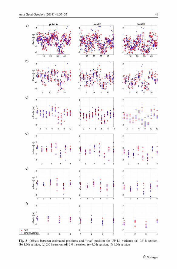
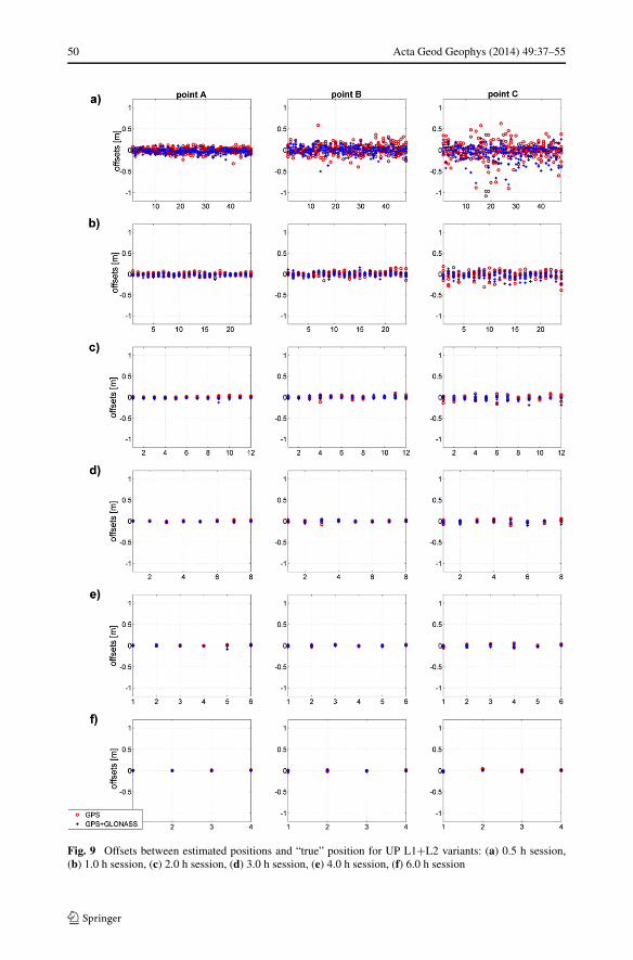
Figures 4–9 present the distribution of differences between estimated positions of the“unknown” points and their corresponding “true” position. The average position from thesix 24-h L1+L2 sessions was adopted as the ‘true’ position. All solution variants wererespectively grouped and presented below.

In Figs. 4–9 the offsets from 24-hour means are presented. It is visible that the largestdifferences occurred for short sessions and, as expected, for variants using only the L1 fre-quency (code-only observations processed). In comparing corresponding figures it is visiblethat the largest offsets for Up component occurred. It is also shown, especially for shortsessions, that the values of offsets increases for points where observations were done un-

Acta Geod Geophys (2014) 49:37–55 45

Fig. 4 Offsets between estimated positions and “true” position for NORTH L1 variants: (a) 0.5 h session,(b) 1.0 h session, (c) 2.0 h session, (d) 3.0 h session, (e) 4.0 h session, (f) 6.0 h session

46 Acta Geod Geophys (2014) 49:37–55

Fig. 5 Offsets between estimated positions and “true” position for NORTH L1+L2 variants: (a) 0.5 h ses-sion, (b) 1.0 h session, (c) 2.0 h session, (d) 3.0 h session, (e) 4.0 h session, (f) 6.0 h session

Acta Geod Geophys (2014) 49:37–55 47

Fig. 6 Offsets between estimated positions and “true” position for EAST L1 variants: (a) 0.5 h session,(b) 1.0 h session, (c) 2.0 h session, (d) 3.0 h session, (e) 4.0 h session, (f) 6.0 h session

48 Acta Geod Geophys (2014) 49:37–55

Fig. 7 Offsets between estimated positions and “true” position for EAST L1+L2 variants: (a) 0.5 h session,(b) 1.0 h session, (c) 2.0 h session, (d) 3.0 h session, (e) 4.0 h session, (f) 6.0 h session

Acta Geod Geophys (2014) 49:37–55 49

Fig. 8 Offsets between estimated positions and “true” position for UP L1 variants: (a) 0.5 h session,(b) 1.0 h session, (c) 2.0 h session, (d) 3.0 h session, (e) 4.0 h session, (f) 6.0 h session

50 Acta Geod Geophys (2014) 49:37–55

Fig. 9 Offsets between estimated positions and “true” position for UP L1+L2 variants: (a) 0.5 h session,(b) 1.0 h session, (c) 2.0 h session, (d) 3.0 h session, (e) 4.0 h session, (f) 6.0 h session

Acta Geod Geophys (2014) 49:37–55 51

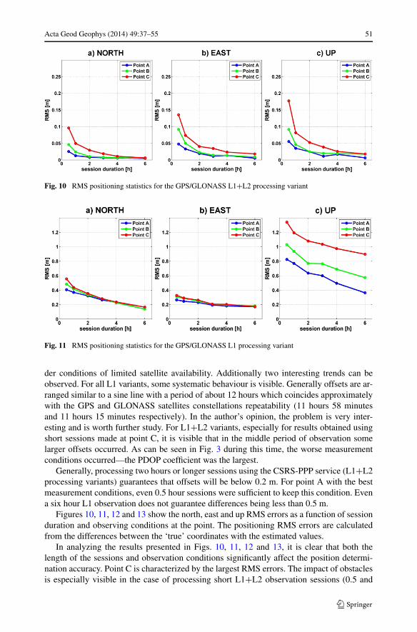
Fig. 10 RMS positioning statistics for the GPS/GLONASS L1+L2 processing variant

Fig. 11 RMS positioning statistics for the GPS/GLONASS L1 processing variant

der conditions of limited satellite availability. Additionally two interesting trends can beobserved. For all L1 variants, some systematic behaviour is visible. Generally offsets are ar-ranged similar to a sine line with a period of about 12 hours which coincides approximatelywith the GPS and GLONASS satellites constellations repeatability (11 hours 58 minutesand 11 hours 15 minutes respectively). In the author’s opinion, the problem is very inter-esting and is worth further study. For L1+L2 variants, especially for results obtained usingshort sessions made at point C, it is visible that in the middle period of observation somelarger offsets occurred. As can be seen in Fig. 3 during this time, the worse measurementconditions occurred—the PDOP coefficient was the largest.

Generally, processing two hours or longer sessions using the CSRS-PPP service (L1+L2processing variants) guarantees that offsets will be below 0.2 m. For point A with the bestmeasurement conditions, even 0.5 hour sessions were sufficient to keep this condition. Evena six hour L1 observation does not guarantee differences being less than 0.5 m.

Figures 10, 11, 12 and 13 show the north, east and up RMS errors as a function of sessionduration and observing conditions at the point. The positioning RMS errors are calculatedfrom the differences between the ‘true’ coordinates with the estimated values.

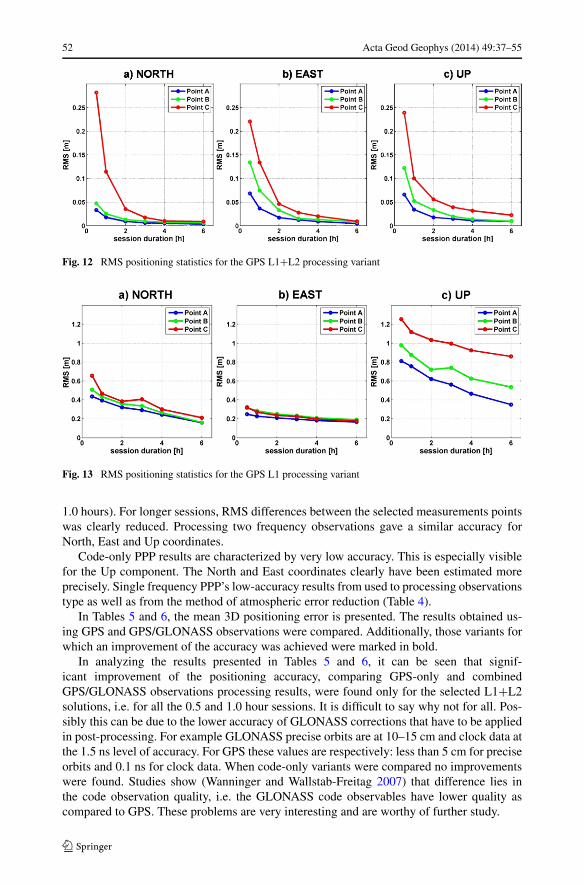
In analyzing the results presented in Figs. 10, 11, 12 and 13, it is clear that both thelength of the sessions and observation conditions significantly affect the position determi-nation accuracy. Point C is characterized by the largest RMS errors. The impact of obstaclesis especially visible in the case of processing short L1+L2 observation sessions (0.5 and

52 Acta Geod Geophys (2014) 49:37–55

Fig. 12 RMS positioning statistics for the GPS L1+L2 processing variant

Fig. 13 RMS positioning statistics for the GPS L1 processing variant

1.0 hours). For longer sessions, RMS differences between the selected measurements pointswas clearly reduced. Processing two frequency observations gave a similar accuracy forNorth, East and Up coordinates.

Code-only PPP results are characterized by very low accuracy. This is especially visiblefor the Up component. The North and East coordinates clearly have been estimated moreprecisely. Single frequency PPP’s low-accuracy results from used to processing observationstype as well as from the method of atmospheric error reduction (Table 4).

In Tables 5 and 6, the mean 3D positioning error is presented. The results obtained us-ing GPS and GPS/GLONASS observations were compared. Additionally, those variants forwhich an improvement of the accuracy was achieved were marked in bold.

In analyzing the results presented in Tables 5 and 6, it can be seen that signif-icant improvement of the positioning accuracy, comparing GPS-only and combinedGPS/GLONASS observations processing results, were found only for the selected L1+L2solutions, i.e. for all the 0.5 and 1.0 hour sessions. It is difficult to say why not for all. Pos-sibly this can be due to the lower accuracy of GLONASS corrections that have to be appliedin post-processing. For example GLONASS precise orbits are at 10–15 cm and clock data atthe 1.5 ns level of accuracy. For GPS these values are respectively: less than 5 cm for preciseorbits and 0.1 ns for clock data. When code-only variants were compared no improvementswere found. Studies show (Wanninger and Wallstab-Freitag 2007) that difference lies inthe code observation quality, i.e. the GLONASS code observables have lower quality ascompared to GPS. These problems are very interesting and are worthy of further study.

Acta Geod Geophys (2014) 49:37–55 53

Table 5 Mean 3D positioning error for L1+L2 variants

Session duration [h] Mean 3D positioning error [m]

Point A Point B Point C

GPS GPS+GLONASS GPS GPS+GLONASS GPS GPS+GLONASS

0.5 0.101 0.078 0.187 0.138 0.431 0.243

1.0 0.053 0.050 0.095 0.072 0.203 0.121

2.0 0.026 0.032 0.048 0.035 0.081 0.072

3.0 0.020 0.017 0.027 0.026 0.051 0.055

4.0 0.015 0.022 0.021 0.025 0.039 0.037

6.0 0.011 0.010 0.014 0.020 0.026 0.026

Table 6 Mean 3D positioning error for L1 variants

Session duration [h] Mean 3D positioning error [m]

Point A Point B Point C

GPS GPS+GLONASS GPS GPS+GLONASS GPS GPS+GLONASS

0.5 0.954 0.917 1.146 1.179 1.452 1.488

1.0 0.882 0.889 1.019 1.064 1.241 1.304

2.0 0.729 0.749 0.843 0.877 1.128 1.166

3.0 0.662 0.685 0.846 0.841 1.098 1.093

4.0 0.555 0.577 0.710 0.752 0.992 1.024

6.0 0.419 0.435 0.590 0.619 0.903 0.928

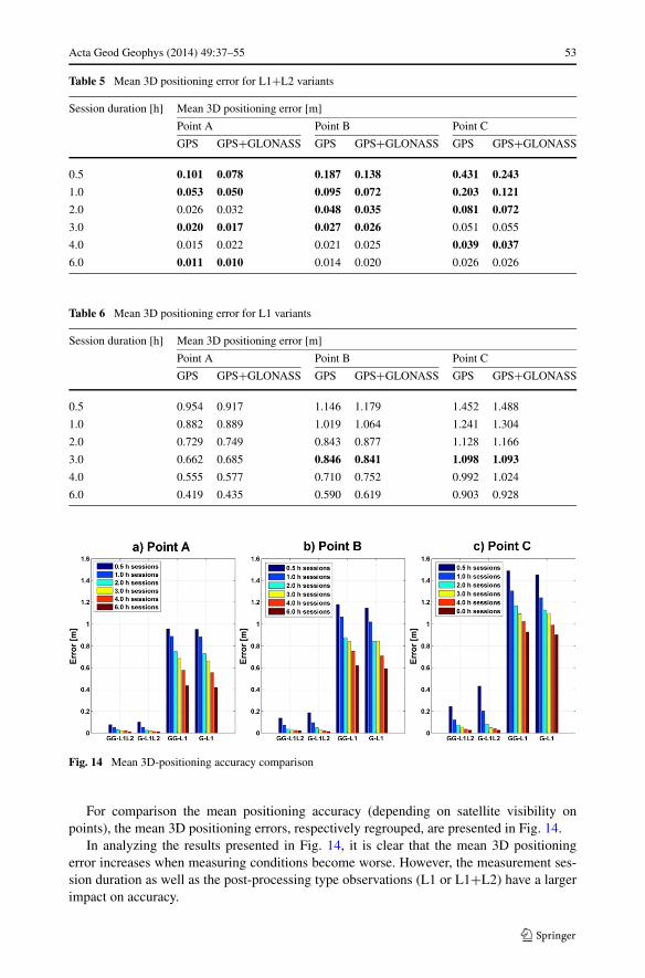
Fig. 14 Mean 3D-positioning accuracy comparison

For comparison the mean positioning accuracy (depending on satellite visibility onpoints), the mean 3D positioning errors, respectively regrouped, are presented in Fig. 14.

In analyzing the results presented in Fig. 14, it is clear that the mean 3D positioningerror increases when measuring conditions become worse. However, the measurement ses-sion duration as well as the post-processing type observations (L1 or L1+L2) have a largerimpact on accuracy.

54 Acta Geod Geophys (2014) 49:37–55

4 Conclusions

In this paper, we analyzed the accuracy of the position determination using single-receiverGNSS measurements taken on points with different observing conditions. The compar-ison also includes the analysis of result differences between GPS only and combinedGPS/GLONASS observations processing as well as an analysis of the position determi-nation accuracy using one and two measurement frequencies. The analysis was based onseven days of data from three GNSS stations. To process the observations, the PPP-CSRSservice was chosen.

The results show that both the length of sessions and observing conditions significantlyaffect the position determination accuracy. The impact of obstacles is especially visible inthe case of processing short observation sessions. For longer sessions, the influence of ob-serving conditions on the accuracy of the position determination was clearly reduced.

Code-only PPP results are characterized by very low accuracy. This is especially visiblefor the Up component. The North and East coordinates have been estimated more precisely.When observations were performed at one frequency in 30 minutes sessions, the precisionof 0.30–0.50 m was achieved for the horizontal coordinates and 0.80–1.30 m for the Upcomponent (RMS). The values improved slightly when the session duration became longerand clearly depend on observing conditions. Adding signals from the GLONASS systemto the post-processing of observation generally worsened the results obtained in all threepoints. This may be due to the lower accuracy of GLONASS code observables as comparedto GPS. Additionally, for all L1 variants some systematic behavior is visible. The calculatedoffsets, in most cases, are arranged similar to a sine line with a period of about 12 hours. Inthe author’s opinion these two problems are worth further study.

In analyzing the results of L1+L2 observations processing, it is clear that under good ob-servation conditions (an unobscured horizon), it is possible to achieve a precision of severalcentimeters after 2 hours of observation. The error for the northing coordinate obtained in thepost-processing of L1+L2 observations is approximately twice smaller than the easting andthe elevation. This occurs in each time variant and it is manifest mainly at point A with thebest measurement conditions and slightly less at point B. In analyzing the results obtainedusing short sessions made at point C, it is clear that in the middle period of observation(the biggest PDOP coefficient values) some larger offsets between estimated positions and“true” position for all coordinates occurred. In comparing GPS-only and GPS/GLONASSsolutions, noticeable improvements for the selected solutions (i.e. for all 0.5 and 1.0 hoursessions) were observed. This is especially true at points with limited horizon visibility(B, C). On the basis of these results, it can be concluded that using GPS/GLONASS obser-vations in PPP may be especially important in processing short static sessions conductedunder conditions of limited satellite availability.

References

Alcay S, Inal C, Yigit CO (2012a) Contribution of GLONASS observations on precise point positioning. In:FIG working week 2012, Rome, Italy, 6–10 May 2012

Alcay S, Inal C, Yigit CO, Yetkin M (2012b) Comparing GLONASS-only with GPS-only and hybrid posi-tioning in various length of baselines. Acta Geod Geophys Hung 47(1):1–12

Bruyninx C (2007) Comparing GPS-only with GPS+GLONASS positioning in a regional permanent GNSSnetwork. GPS Solut 11(2):97–106

Cai C, Gao Y (2007) Precise point positioning using combined GPS and GLONASS observations. J GlobPosition Syst 6(1):13–22

Acta Geod Geophys (2014) 49:37–55 55

Choy S (2011) High accuracy precise point positioning using a single frequency GPS receiver. J Appl Geod5:59–69

Dawidowicz K (2013) Impact of different GNSS antenna calibration models on height determination in theASG-EUPOS network—a case study. Surv Rev 45(332):386–394

Dodson AH, Moore T, Baker FD, Swann JW (1999) Hybrid GPS+GLONASS. GPS Solut 3(1):32–41Ebner R, Featherstone WE (2008) How well can online GPS PPP post-processing services be used to establish

geodetic survey control networks? J Appl Geod 2(3):149–157Elsobeiey M, El-Rabbany A (2011) Impact of second-order ionospheric delay on GPS precise point position-

ing. J Appl Geod 5:37–45Gao Y (2006) Precise point positioning and its challenges, aided-GNSS and signal tracking. Inside GNSS

1(8):16–18Gao Y, Kongzhe C (2004) Performance analysis of precise point positioning using real-time orbit and clock

products. J Glob Position Syst 3(1–2):95–100Gao Y, Abdel-Salam M, Chen K, Wojciechowski A (2005) Point real-time kinematic positioning. In: A win-

dow on the future of geodesy. International association of geodesy symposia, vol 128, pp 77–82Ge M, Gendt G, Rothacher M, Shi C, Geng J, Liu J (2008) Resolution of GPS carrier-phase ambiguities in

PPP with daily observations. J Geod 82(7):389–399Geng J, Meng X, Dodson AH, Teferle FN (2010) Integer ambiguity resolution in precise point positioning:

method comparison. J Geod 84(9):569–581Grinter T, Janssen V (2012) Post-processed precise point positioning: a viable alternative? In: Proc

APAS2012, Wollongong, Australia, 19–21 March, pp 83–92Hadas T, Kaplon J, Bosy J, Sierny J, Wilgan K (2013) Near-real-time regional troposphere models for

the GNSS precise point positioning technique. Meas Sci Technol 24(5). doi:10.1088/0957-0233/24/5/055003

Hofmann-Wellenhof B, Lichtenegger H, Wasle E (2008) GNSS–GPS, GLONASS, Galileo & more. Springer,Wien

Kouba J, Héroux P (2001) Precise point positioning using IGS orbit and clock products. GPS Solut 5(2):12–28

Moreno B, Radicella SC, de Lacy S, Herraiz M, Rodriguez-Caderot G (2011) On the effects of the ionosphericdisturbances on precise point positioning at equatorial latitudes. GPS Solut 15:381–390

Nejat D, Kiamehr R (2013) An investigation on accuracy of DGPS network-based positioning in moun-tainous regions, a case study in Alborz network. Acta Geod Geophys 48:39–51. doi:10.1007/s40328-012-0003-3

Oleynik EG, Mitrikas VV, Revnivykh SG, Serdukov AI, Dutov EN, Shiriaev VF (2006) High-accurateGLONASS orbit and clock determination for the assessment of system performance. In: Proceedings ofION GNSS 2006, Fort Worth, TX, September 26–29

Parkinson B, Spilker JJ (1996) Global positioning system: theory and applications, vol I. American Instituteof Aeronautics and Astronautics, Inc, Washington

Rizos C, Janssen V, Roberts C, Grinter T (2012) Precise point positioning: is the era of differential GNSSpositioning drawing to an end? In: FIG working week 2012, Rome, Italy

Seeber G (2003) Satellite geodesy. de Gruyter, BerlinSnay RA, Soler T (2008) Continuously operating reference station (CORS): history, applications, and future

enhancements. J Surv Eng 134(4):95–104Wanninger L, Wallstab-Freitag S (2007) Combined processing of GPS, GLONASS and SBAS code phase and

carrier phase measurements. In: Proc ION GNSS 2007, Fort Worth, Tx, September 25–28, pp 866–875Weber R, Slater JA, Fragner E, Glotov V, Habrich H, Romero I, Schaer S (2005) Precise GLONASS orbit

determination within the IGS/IGLOS pilot project. Adv Space Res 36:369–375Wielgosz P, Cellmer S, Rzepecka Z, Paziewski J, Grejner-Brzezinska D (2011) Troposphere modeling for

precise GPS rapid static positioning in mountainous areas. Meas Sci Technol 22(4):45101–45109Zumberge JF, Heflin MB, Jefferson DC, Watkins MM, Webb FH (1997) Precise point positioning for the

efficient and robust analysis of GPS data from large networks. J Geophys Res 3(102):5005–5017