Cooperative Planning for Coupled Multi-Agent Systems under TimedTemporal Specifications

Alexandros Nikou, Dimitris Boskos, Jana Tumova and Dimos V. Dimarogonas

Abstract— This paper presents a fully automated procedurefor controller synthesis for multi-agent systems under coupledconstraints. Each agent has dynamics consisting of two terms:the first one models the coupled constraints and the other oneis an additional control input. We aim to design these inputsso that each agent meets an individual high-level specificationgiven as a Metric Interval Temporal Logic (MITL). First,a decentralized abstraction that provides a time and spacediscretization of the multi-agent system is designed. Second,by utilizing this abstraction and techniques from formal veri-fication, we provide an algorithm that computes the individualruns which provably satisfy the high-level tasks. The overallapproach is demonstrated in a simulation example.

I. INTRODUCTION

Cooperative control of multi-agent systems has tradition-ally focused on designing distributed control laws in orderto achieve global tasks such as consensus, formation andrendez-vous ([1]–[5]) and at the same time fulfill propertiessuch as network connectivity ([6], [7]). Over the last fewyears, multi-agent control under complex high-level specifi-cations has been gaining significant attention. In particular,coordination of multi-robot teams under qualitative temporaltasks constitutes an emerging application in this field. In thiswork, we aim to additionally introduce specific time boundsinto these tasks, in order to include specifications such as“Visit region A within 5 time units” or “Periodically surveyregions A1, A2, A3, avoid region X and always keep thelongest time between two consecutive visits to A1 below 20time units”.

The specification language that has primarily been usedto express the tasks is Linear Temporal Logic (LTL) (see,e.g., [8]). LTL has been proven a valuable tool for controllersynthesis, because it provides a compact mathematical for-malism for specifying desired behaviors of a system. There isa rich body of literature containing algorithms for verificationand synthesis of multi-agent systems under temporal logicspecifications ([9], [10]). A common approach in multi-agentplanning under LTL specifications is the consideration of acentralized, global task for the team, which is then decom-posed into local tasks to be accomplished by the individualagents (see [11], [12]). A three-step hierarchical procedure toaddress this problem is described as follows ([13]): first, therobot dynamics is abstracted into a discrete transition systemusing sampling or cell decomposition methods based on

The authors are with the ACCESS Linnaeus Center, School of ElectricalEngineering, KTH Royal Institute of Technology, SE-100 44, Stockholm,Sweden and with the KTH Center for Autonomous Systems. Email:anikou, boskos, tumova, dimos@kth.se. This workwas supported by the H2020 ERC Starting Grant BUCOPHSYS, theSwedish Research Council (VR) and the Knut och Alice WallenbergFoundation.

triangular, rectangular or other partitions. Second, invokingideas from formal verification, a discrete plan that meetsthe high-level task is synthesized. Third, the discrete planis translated into a sequence of continuous controllers forthe original system.

Time constraints in the system modeling have been con-sidered e.g., in [14]–[16]. Both the aforementioned, as wellas most existing works on multi-agent planning, considertemporal properties which treat time in a qualitative manner.However, for real applications, a multi-agent team might berequired to perform a specific task within a certain timebound, rather than at some arbitrary time in the future, i.e. ina quantitative manner. Timed specifications have been con-sidered in [17]–[21]. However, all these works are restrictedto single agent planning and they are not extendable to multi-agent systems in a straightforward way.

The multi-agent case has been considered in [22], wherethe vehicle routing problem was addressed, under MetricTemporal Logic (MTL) specifications. The correspondingapproach does not rely on automata-based verification, as it isbased on a construction of linear inequalities and the solutionof a Mixed-Integer Linear Programming (MILP) problem.An automata-based solution was proposed in our previouswork [23], where Metric Interval Temporal Logic (MITL)formulas were introduced in order to synthesize controllerssuch that every agent fulfills an individual specification andthe team of agents fulfill a global specification.

In [23], the abstraction of the dynamics was given andan upper bound of the time that each agent needs to finisha transition from one region to another was assumed. Fur-thermore, potential coupled constraints between the agentswere not taken into consideration. In this work, we aim toaddress the aforementioned issues. The dynamics of eachagent consists of two parts: the first part is a consensus typeterm representing the coupling between the agent and itsneighbors, and the second one is an additional control inputwhich will be exploited for high-level planning. Hereafter, itwill be called a free input. A decentralized abstraction pro-cedure is provided, which leads to an individual TransitionSystem (TS) for each agent and provides the basis for high-level planning. Additionally, this abstraction is associated toa time quantization which allows us to assign precise timedurations to the transitions of each agent.

There is a rich literature on abstractions for dynamical sys-tems (see e.g., [24]–[27]). Multi-agent abstractions have beenaddressed in [28]–[32]. Motivated by [32], we start from thedynamics of each agent and we construct a TS for each agentin a decentralized manner. An individual task is assigned toeach agent and we aim to design the free inputs so that each

agent performs the desired individual task within specifictime bounds. To the best of the authors’ knowledge, this isthe first time that a fully automated framework for multi-agent systems consisting of both constructing an abstractionand conducting high-level timed temporal logic planning isconsidered. Hence, this works lies in the intersection of thefields of multi-agent systems, abstractions and timed formalverification.

The contribution of this paper is to provide an automaticcontroller synthesis method of a general framework of cou-pled multi-agent systems under high-level tasks with timedconstraints. Compared to the existing works on multi-agentplanning under temporal logic specifications, the proposedapproach yields the first solution to the problem of planningof dynamically coupled multi-agent systems under timedtemporal specifications in a distributed way.

The remainder of the paper is structured as follows. InSec. II a description of the necessary mathematical tools, thenotations and the definitions are given. Sec. III provides thedynamics of the system and the formal problem statement.Sec. IV discusses the technical details of the solution. Sec. Vis devoted to a simulation example. Finally, the conclusionsand the future work directions are discussed in Sec. VI.

II. NOTATION AND PRELIMINARIES

A. NotationWe denote by R,Q+,N the set of real, nonnegative

rational and natural numbers including 0, respectively. Also,define T∞ = T ∪ ∞ for a set T ⊆ R. Given a set S,we denote by |S| its cardinality and by 2S the set of all itssubsets. For a subset S of Rn, we denote by cl(S), int(S)and ∂S = cl(S)\int(S) its closure, interior and boundary,respectively and \ is used for set subtraction. The notation‖x‖ is used for the Euclidean norm of a vector x ∈ Rn and‖A‖ = max‖Ax‖ : ‖x‖ = 1 for the induced norm of amatrix A ∈ Rm×n. Given a matrix A, the spectral radius ofA is denoted by λmax(A) = max|λ| : λ ∈ σ(A), whereσ(A) is the set of all the eigenvalues of A.

B. Multi-Agent SystemsConsider a set of agents I = 1, 2, . . . , N operating in

Rn. The topology of the multi-agent network is modeledthrough a static undirected graph G = (I, E), where I isthe set of nodes (agents) and E ⊆ i, j : i, j ∈ I, i 6= jis the set of edges (denoting the communication capabilitybetween neighboring respective agents). For each agent, itsneighbors’ set N (i) is defined as N (i) = j1, . . . , jNi =j ∈ I : i, j ∈ E where Ni = |N (i)|.

Given a vector xi = (x1i , . . . , x

ni ) ∈ Rn, the component

operator c(xi, k) = xki ∈ R, k = 1, . . . , n gives theprojection of xi onto its k-th component (see [33]). Similarly,for the stack vector x = (x1, . . . , xN ) ∈ RNn the componentoperator is defined as c(x, k) = (c(x1, k), . . . , c(xN , k))∈ RN , k = 1, . . . , n. By using the component operator, thenorm of a vector x ∈ RNn can be computed as ‖x‖ =∑n

k=1 ‖c(x, k)‖2 1

2 .The Laplacian matrix L(G) ∈ RN×N of the graph G

is defined as L(G) = D(G)D(G)τ where D(G) is the

N × |E| incidence matrix ([33]). The graph Laplacian L(G)is positive semidefinite and symmetric. By considering anordering 0 = λ1(G) ≤ λ2(G) ≤ . . . ≤ λN (G) = λmax(G) ofthe eigenvalues of L(G) then we have that λ2(G) > 0 iff Gis connected ([33]).

We denote by x ∈ R|E|n the stack column vector of thevectors xi − xj , i, j ∈ E with the edges ordered as in thecase of the incidence matrix. Thus, the following holds:

x = D(G)τx. (1)

C. Cell DecompositionsIn the subsequent analysis a discrete partition of the

workspace into cells will be considered which is formalizedthrough the following definition.

Definition 1. A cell decomposition S = S``∈I of a setD ⊆ Rn, where I ⊆ N is a finite or countable index set, isa family of uniformly bounded convex sets S`, ` ∈ I suchthat int(S`) ∩ int(Sˆ) = ∅ for all `, ˆ ∈ I with ` 6= ˆ and∪`∈IS` = D.

Example 1. An example of a cell decomposition with I =1, 2, 3, 4, 5, 6 and S = S``∈I = S1, S2, S3, S4, S5, S6is depicted in Fig. 1. This cell decomposition will be usedas reference for the following examples.

S1 S2 S3

S4S5S6

Fig. 1: An example of a cell decomposition with |I| = 6cells

D. Time Sequence, Timed Run and Weighted TransitionSystem

In this section we review some basic definitions fromcomputer science that are required in the sequel.

An infinite sequence of elements of a set X is calledan infinite word over this set and it is denoted by χ =χ(0)χ(1) . . . The i-th element of a sequence is denoted byχ(i).

Definition 2. ([34]) A time sequence τ = τ(0)τ(1) . . . is aninfinite sequence of time values τ(j) ∈ T = Q+, satisfyingthe following properties:• Monotonicity: τ(j) < τ(j + 1) for all j ≥ 0.• Progress: For every t ∈ T, there exists j ≥ 1, such thatτ(j) > t.

An atomic proposition p is a statement that is either True(>) or False (⊥).

Definition 3. ([34]) Let AP be a finite set of atomic proposi-tions. A timed word w over the set AP is an infinite sequencewt = (w(0), τ(0))(w(1), τ(1)) . . . where w(0)w(1) . . . is aninfinite word over the set 2AP and τ(0)τ(1) . . . is a timesequence with τ(j) ∈ T, j ≥ 0.

Definition 4. A Weighted Transition System (WTS) is a tuple(S, S0, Act,−→, d, AP,L) where S is a finite set of states;S0 ⊆ S is a set of initial states; Act is a set of actions; −→⊆S×Act×S is a transition relation; d :−→→ T is a map thatassigns a positive weight (time values in this framework) toeach transition; AP is a finite set of atomic propositions;and L : S → 2AP is a labeling function. For simplicity, thenotation s

α−→ s′ is used to denote that (s, α, s′) ∈−→ fors, s′ ∈ S and α ∈ Act. Furthermore, for every s ∈ S andα ∈ Act the operator Post(s, α) = s′ ∈ S : (s, α, s′) ∈−→ is defined.

Definition 5. A timed run of a WTS is an infinite sequencert = (r(0), τ(0))(r(1), τ(1)) . . ., such that r(0) ∈ S0, andfor all j ≥ 1, it holds that r(j) ∈ S and (r(j), α(j), r(j +1)) ∈−→ for a sequence of actions α(1)α(2) . . . with α(j) ∈Act,∀ j ≥ 1. The time stamps τ(j), j ≥ 0 are inductivelydefined as

1) τ(0) = 0.2) τ(j + 1) = τ(j) + d(r(j), r(j + 1)), ∀ j ≥ 1.

Every timed run rt generates a timed word w(rt) =(w(0), τ(0)) (w(1), τ(1)) . . . over the set 2AP where w(j) =L(r(j)), ∀ j ≥ 0 is the subset of atomic propositions thatare true at state r(j).

E. Metric Interval Temporal Logic

The syntax of Metric Interval Temporal Logic (MITL) overa set of atomic propositions AP is defined by the grammar

ϕ := p | ¬ϕ | ϕ1∧ϕ2 | ©I ϕ | ♦Iϕ | Iϕ | ϕ1 UI ϕ2 (2)

where p ∈ AP , and ©, ♦, and U are the next,eventually, always and until temporal operator, respectively.I ⊆ T is a non-empty time interval in one of the followingforms: [i1, i2], [i1, i2), (i1, i2], (i1, i2), [i1,∞], (i1,∞) wherei1, i2 ∈ T with i1 < i2. MITL can be interpreted either incontinuous or point-wise semantics [35]. The latter approachis utilized, since the consideration of point-wise (event-base) type semantics renders a framework that includesTransition Systems and automata construction, namely ourcurrent approach, more natural. The MITL formulas areinterpreted over timed runs such as the ones produced bya WTS (Def. 5).

Definition 6. ([35], [36]) Given a timed word wt =(w(0), τ(0))(w(1), τ(1)) . . . and an MITL formula ϕ, wedefine (wt, i) |= ϕ, for i ≥ 0 (read wt satisfies ϕ at positioni) as follows:

(wt, i) |= p⇔ p ∈ w(i)

(wt, i) |= ¬ϕ⇔ (wt, i) 6|= ϕ

(wt, i) |= ϕ1 ∧ ϕ2 ⇔ (wt, i) |= ϕ1 and (wt, i) |= ϕ2

(wt, i) |=©I ϕ⇔ (wt, i+ 1) |= ϕ and τ(i+ 1)− τ(i) ∈ I(wt, i) |= ♦Iϕ⇔ ∃j ≥ i, s.t. (wt, j) |= ϕ, τ(j)− τ(i) ∈ I(wt, i) |= Iϕ⇔ ∀j ≥ i, τ(j)− τ(i) ∈ I ⇒ (wt, j) |= ϕ

(wt, i) |= ϕ1 UI ϕ2 ⇔ ∃j ≥ i, s.t. (wt, j) |= ϕ2,

τ(j)− τ(i) ∈ I and (wt, k) |= ϕ1 for every i ≤ k < j.

It has been proved that MITL is decidable in both finiteand infinite words [37] and in both pointwise and contin-uous semantics [38]. The model checking and satisfiabilityproblems are EXPSPACE-complete.

s0 s1 s2

1.0

2.0

1.5

0.5

Fig. 2: An example of a WTS

Example 2. Consider the WTS T with S =s0, s1, s2, S0 = s0, Act = ∅,−→= (s0, ∅, s1),(s1, ∅, s2), (s1, ∅, s0), (s2, ∅, s1), d((s0, ∅, s1)) =1.0, d((s1, ∅, s2)) = 1.5, d((s1, ∅, s0)) = 2.0,d((s2, ∅, s1)) = 0.5, AP = green, L(s0) =green, L(s1) = L(s2) = ∅ depicted in Fig. 2.

Let two timed runs of the system: rt1 =(s0, 0.0)(s1, 1.0)(s0, 3.0)(s1, 4.0) . . . , rt2 =(s0, 0.0)(s1, 1.0)(s2, 2.5)(s1, 3.0) . . . and two MITLformulas ϕ1 = ♦[2,5]green, ϕ2 = [0,5]green.According to the MITL semantics, it can be seen that thetimed run rt1 satisfies the formula ϕ1 (we formally writert1 |= ϕ1), since at the time stamp 3.0 ∈ [2, 5] we have thatL(s0) = green so the atomic proposition green occursat least once in the given interval. On the other hand, thetimed run rt2 does not satisfy the formula ϕ2 (we formallywrite rt2 6|= ϕ2) since the atomic proposition green does notalways hold at every time stamp of the runs (it holds onlyat the time stamp 0.0).

F. Timed Buchi Automata

Timed Buchi Automata (TBA) were introduced in [34]. Inthis work, the notation from [39], [40] is partially adopted.Let C = c1, . . . , c|C| be a finite set of clocks. The set ofclock constraints Φ(C) is defined by the grammar

φ := > | ¬φ | φ1 ∧ φ2 | c ./ ψ (3)

where c ∈ C is a clock, ψ ∈ T is a clock constant and./ ∈ <,>,≥,≤,=. An example of clock constraints for aset of clocks C = c1, c2 can be Φ(C) = c < c1∨c > c2.A clock valuation is a function ν : C → T that assigns avalue to each clock. A clock ci has valuation νi for i ∈1, . . . , |C|, and ν = (ν1, . . . , ν|C|). By ν |= φ is denotedthe fact that the valuation ν satisfies the clock constraint φ.

Definition 7. A Timed Buchi Automaton is a tuple A =(Q,Qinit, C, Inv,E, F,AP,L) where Q is a finite set oflocations; Qinit ⊆ Q is the set of initial locations; C isa finite set of clocks; Inv : Q → Φ(C) is the invariant;E ⊆ Q × Φ(C) × 2C × Q gives the set of edges; F ⊆ Qis a set of accepting locations; AP is a finite set of atomicpropositions; and L : Q → 2AP labels every state with asubset of atomic propositions.

A state of A is a pair (q, ν) where q ∈ Q and ν satisfiesthe invariant Inv(q), i.e., ν |= Inv(q). The initial stateof A is (q(0), (0, . . . , 0)), where q(0) ∈ Qinit. Given two

states (q, ν) and (q′, ν′) and an edge e = (q, γ,R, q′), thereexists a discrete transition (q, ν)

e−→ (q′, ν′) iff ν |= γ,ν′ |= Inv(q′), and R is the reset set, i.e., ν′i = 0 for ci ∈ Rand ν′i = νi for ci /∈ R. Given a δ ∈ T, there exists atime transition (q, ν)

δ−→ (q′, ν′) iff q = q′, ν′ = ν + δ(δ is summed component-wise) and ν′ |= Inv(q). Wewrite (q, ν)

δ−→ e−→ (q′, ν′) if there exists q′′, ν′′ such that(q, ν)

δ−→ (q′′, ν′′) and (q′′, ν′′)e−→ (q′, ν′) with q′′ = q.

An infinite run of A starting at state (q(0), ν) is an infinitesequence of time and discrete transitions (q(0), ν(0))

δ0−→(q(0)′, ν(0)′)

e0−→ (q(1), ν(1))δ1−→ (q(1)′, ν(1)′) . . ., where

(q(0), ν(0)) is an initial state. This run produces the timedword w = (L(q(0)), τ(0))(L(q(1)), τ(1)) . . . with τ(0) = 0and τ(i+1) = τ(i)+δi, ∀ i ≥ 1. The run is called acceptingif q(i) ∈ F for infinitely many times. A timed word isaccepted if there exists an accepting run that produces it.The problem of deciding the emptiness of the language of agiven TBA A is PSPACE-complete [34]. In other words, anaccepting run of a given TBA A can be synthesized, if oneexists.

Any MITL formula ϕ over AP can be algorithmicallytranslated to a TBA with the alphabet 2AP , such that thelanguage of timed words that satisfy ϕ is the language oftimed words produced by the TBA ([37], [41], [42]).

Example 3. The TBA A with Q = q0, q1, q2, Qinit =q0, C = c, Inv(q0) = Inv(q1) = Inv(q2) = ∅, E =(q0, c ≤ c2, ∅, q0), (q0, c ≤ c1∨c > c2, c, q2), (q0, c ≥c1 ∧ c ≤ c2, c, q1), (q1,>, c, q1), (q2,>, c, q2), F =q1, AP = green,L(q0) = L(q2) = ∅,L(q1) =green that accepts all the timed words that satisfy theformula ϕ = ♦[c1,c2]green is depicted in Fig. 3. Thisformula will be used as reference for the following examplesand simulations.

q0 q1

q2

>, c := 0

>, c := 0

c ≤ c2, ∅

c ≥ c1 ∧ c ≤ c2c := 0

c < c1 ∨ c > c2c := 0

green

Fig. 3: A TBA A that accepts the runs that satisfy formulaϕ = ♦[c1,c2]green.

An example of a timed run of this TBA is(q0, 0)

δ=α1−→ (q0, α1)e=(q0,c≥c1∧c≤c2,c,q1)−→ (q1, 0) . . .

with c1 ≤ α1 ≤ c2, which generates the timedword wt = (L(q0), 0)(L(q0), α1)(L(q1), α1) . . . =(∅, 0)(∅, α1)(green, α1) . . . that satisfies the formula ϕ.

The timed run (q0, 0)δ=α2−→ (q0, α2)

e=(q0,c≤c1∨c>c2,c,q2)−→ (q2, 0) . . . with α2 < c1, generatesthe timed word wt = (L(q0), 0)(L(q0), α2)(L(q2), α2) . . . = (∅, 0)(∅, α2)(∅, α2) . . . that does notsatisfy the formula ϕ.

III. PROBLEM FORMULATION

A. System Model

We focus on multi-agent systems with coupled dynamicsof the form

xi = −∑

j∈N (i)

(xi − xj) + vi, xi ∈ Rn, i ∈ I. (4)

where vi ∈ Rn, i ∈ I. The dynamics (4) consists of twoparts; the first part is a consensus protocol representing thecoupling between the agent and its neighbors, and the secondone is a control input which will be exploited for high-levelplanning and is called free input. In this work, it is assumedthat the free inputs are bounded by a positive constant vmax.Namely, ‖vi(t)‖ ≤ vmax, ∀ i ∈ I, t ≥ 0.

Assumption 1. We assume that the communication graphG = (I, E) of the system is undirected and static i.e., everyagent preserves the same neighbors for all times.

Notice that the system (4) can be also expressed in theform c(x, k) = −L(G) c(x, k) + c(v, k), k ∈ 1, . . . , nwhere x, v ∈ RNn are obtained by invoking the definitionof the component operator from Sec. II-B.

B. Specification

Our goal is to control the multi-agent system (4) sothat each agent obeys a given individual specification. Inparticular, it is required to drive each agent to a sequenceof desired subsets of the workspace Rn within certain timelimits and provide certain atomic tasks there. Atomic tasksare captured through a finite set of services Σi, i ∈ I. Hence,it is desired to relate the position xi of each agent i ∈ I in theworkspace with the services that are offered at xi. Initially,a labeling function

Λi : Rn → 2Σi (5)

is introduced for each agent i ∈ I which maps each statexi ∈ Rn to the subset of services Λi(xi) which hold trueat xi i.e., the subset of services that agent i can provide inposition xi. It should be noted that although the term labelingfunction it is used, these functions should not be confusedwith the labeling functions of a WTS as in Definition 4. Theunion of all the labeling functions as Λ(x) =

⋃i∈I Λi(x) is

also defined.Without loss of generality, we assume that Σi∩Σj = ∅, for

all i, j ∈ I, i 6= j which means that the agents do not shareany services. Let us now introduce the following assumptionwhich is important for defining the problem properly.

Assumption 2. There exists a partition S = S``∈I of theworkspace which forms a cell decomposition according toDefinition 1 and respects the labeling function Λ i.e., forall S` ∈ S it holds that Λ(x) = Λ(x′),∀ x, x′ ∈ S`. This

assumption intuitively and again without loss of generality,means that the same services hold at all the points that belongto the same cell of the partition.

Define now for each agent i ∈ I a labeling function

Li : S → 2Σi (6)

which denotes the fact that when agent i visits a region S` ∈S, it chooses to provide a subset of services that are beingoffered there i.e., it chooses to satisfy a subset of Li(S`).

The trajectory of each agent i is denoted byxi(t), t ≥ 0, i ∈ I. The trajectory xi(t), i ∈ Iis associated with a unique sequence rtxi =(ri(0), τi(0))(ri(1), τ1(1))(ri(2), τi(2)) . . . of regions thatthe agent i crosses, where for all j ≥ 0, ri(j) ∈ S` for some` ∈ I, Λi(xi(t)) = Li(ri(j)),∀ t ∈ [τi(j), τi(j + 1)) andri(j) 6= ri(j + 1). The equality Λi(·) = Li(·), i ∈ Iis feasible due to assumption 2. The timed wordwtxi = (wi(0), τi(0))(wi(1), τi(1))(wi(2), τi(2)) . . ., wherewi(j) = Li(ri(j)), j ≥ 0, i ∈ I, is associated uniquely withthe trajectory xi(t) and represents the sequence of servicesthat can be provided by the agent i following the trajectoryxi(t), t ≥ 0.

We define the timed service word as

wtxi = (βi(z0), τi(z0))(βi(z1), τi(z1))(βi(z2), τi(z2)) . . .(7)

where z0 = 0 < z1 < z2 < . . . is a sequence of integers,and for all j ≥ 0 it holds that βi(zj) ⊆ Li(ri(zj)) andτ(zj) ∈ [τi(zj), τi(zj + 1)). The timed service word is asequence of services that are actually provided by agent iand it is compliant with the trajectory xi(t), t ≥ 0.

The specification task ϕi given in MITL formulas over theset of services Σi as in Definition 6, captures requirementson the services to be provided by agent i for each i ∈ I.We say that a trajectory xi(t) satisfies a given formula ϕiin MITL over the set of atomic propositions Σi if and onlyif there exits a timed service word, as defined in (7), thatcomplies with xi(t) and satisfies ϕi according to Definition6.

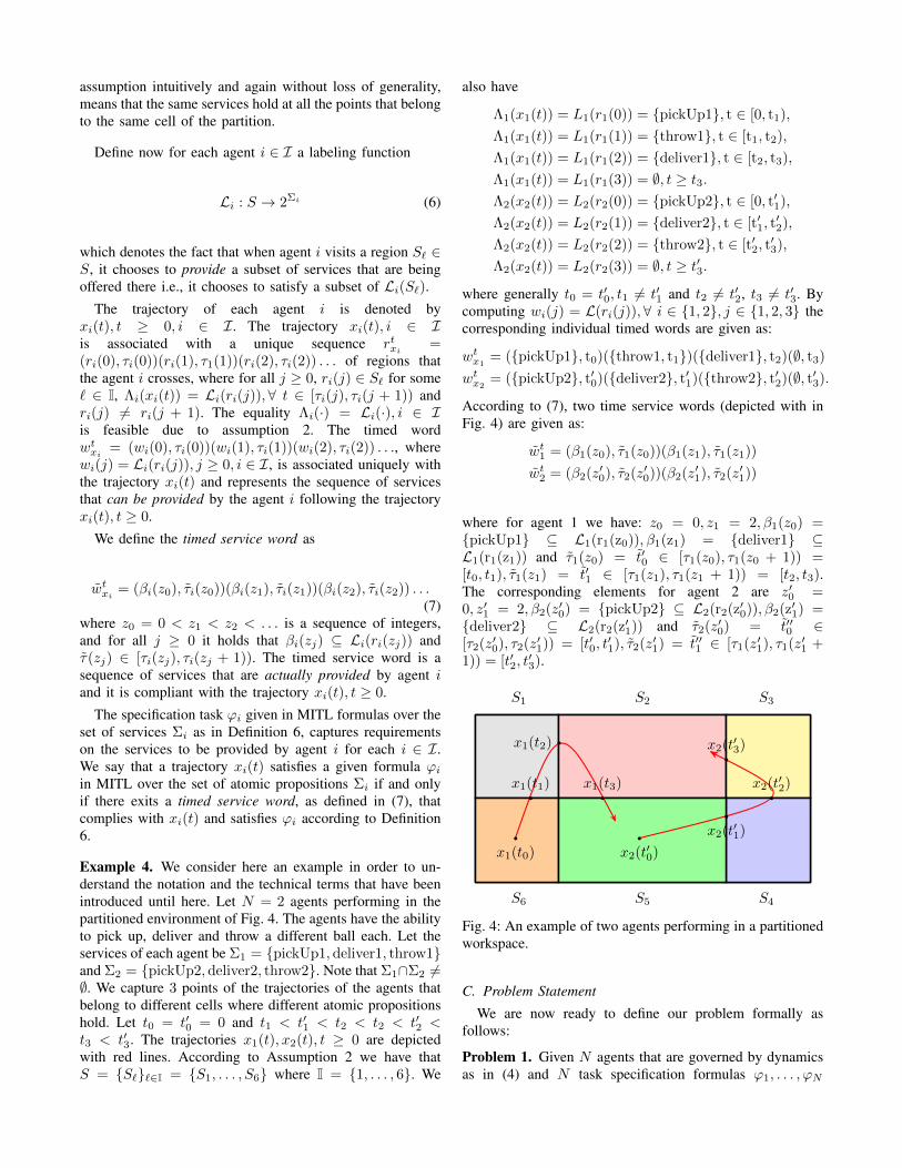
Example 4. We consider here an example in order to un-derstand the notation and the technical terms that have beenintroduced until here. Let N = 2 agents performing in thepartitioned environment of Fig. 4. The agents have the abilityto pick up, deliver and throw a different ball each. Let theservices of each agent be Σ1 = pickUp1,deliver1, throw1and Σ2 = pickUp2,deliver2, throw2. Note that Σ1∩Σ2 6=∅. We capture 3 points of the trajectories of the agents thatbelong to different cells where different atomic propositionshold. Let t0 = t′0 = 0 and t1 < t′1 < t2 < t2 < t′2 <t3 < t′3. The trajectories x1(t), x2(t), t ≥ 0 are depictedwith red lines. According to Assumption 2 we have thatS = S``∈I = S1, . . . , S6 where I = 1, . . . , 6. We

also have

Λ1(x1(t)) = L1(r1(0)) = pickUp1, t ∈ [0, t1),

Λ1(x1(t)) = L1(r1(1)) = throw1, t ∈ [t1, t2),

Λ1(x1(t)) = L1(r1(2)) = deliver1, t ∈ [t2, t3),

Λ1(x1(t)) = L1(r1(3)) = ∅, t ≥ t3.Λ2(x2(t)) = L2(r2(0)) = pickUp2, t ∈ [0, t′1),

Λ2(x2(t)) = L2(r2(1)) = deliver2, t ∈ [t′1, t′2),

Λ2(x2(t)) = L2(r2(2)) = throw2, t ∈ [t′2, t′3),

Λ2(x2(t)) = L2(r2(3)) = ∅, t ≥ t′3.

where generally t0 = t′0, t1 6= t′1 and t2 6= t′2, t3 6= t′3. Bycomputing wi(j) = L(ri(j)),∀ i ∈ 1, 2, j ∈ 1, 2, 3 thecorresponding individual timed words are given as:

wtx1= (pickUp1, t0)(throw1, t1)(deliver1, t2)(∅, t3)

wtx2= (pickUp2, t′0)(deliver2, t′1)(throw2, t′2)(∅, t′3).

According to (7), two time service words (depicted with inFig. 4) are given as:

wt1 = (β1(z0), τ1(z0))(β1(z1), τ1(z1))

wt2 = (β2(z′0), τ2(z′0))(β2(z′1), τ2(z′1))

where for agent 1 we have: z0 = 0, z1 = 2, β1(z0) =pickUp1 ⊆ L1(r1(z0)), β1(z1) = deliver1 ⊆L1(r1(z1)) and τ1(z0) = t′0 ∈ [τ1(z0), τ1(z0 + 1)) =[t0, t1), τ1(z1) = t′1 ∈ [τ1(z1), τ1(z1 + 1)) = [t2, t3).The corresponding elements for agent 2 are z′0 =0, z′1 = 2, β2(z′0) = pickUp2 ⊆ L2(r2(z′0)), β2(z′1) =deliver2 ⊆ L2(r2(z′1)) and τ2(z′0) = t′′0 ∈[τ2(z′0), τ2(z′1)) = [t′0, t

′1), τ2(z′1) = t′′1 ∈ [τ1(z′1), τ1(z′1 +

1)) = [t′2, t′3).

x1(t0)

x1(t1)

x1(t2)

x1(t3) x2(t′2)

x2(t′1)

x2(t′0)

x2(t′3)

S1 S2 S3

S4S5S6

Fig. 4: An example of two agents performing in a partitionedworkspace.

C. Problem Statement

We are now ready to define our problem formally asfollows:

Problem 1. Given N agents that are governed by dynamicsas in (4) and N task specification formulas ϕ1, . . . , ϕN

expressed in MITL over the sets of services Σ1, . . . ,ΣN ,respectively, the partition S = S``∈I as in Assumption2 and the labeling functions Λ1, . . . ,ΛN and L1, . . . ,LN ,as in (5), (6) respectively, assign control laws to the freeinputs v1, . . . , vN such that each agent fulfills its individualspecification, given the bound vmax.

Remark 1. In our preliminary work on the multi-agentcontroller synthesis framework under MITL specifications[23], the multi-agent system was considered to have fully-actuated dynamics. The only constraints on the system weredue to the presence of time constrained MITL formulas. Inthe current framework, we have two types of constraints.Primarily, due to the coupled dynamics of the system, whichconstrain the motion of each agent, and, secondly, the timedconstraints that are inherently imposed from the time boundsof the MITL formulas. Thus, there exist formulas that cannotbe satisfied either due to the coupling constraints or thetime constraints of the MITL formulas. These constraints,make the procedure of the controller synthesis in the discretelevel substantially different and more elaborate than thecorresponding multi-agent LTL frameworks in the literature([9]–[12]).

Remark 2. It should be noted here that, in this work,the couplings and the dependencies between the agents aretreated by the dynamics of the form (4) and not in the discretelevel by coupling also in the services of each agent (i.e.,Σi ∩ Σj 6= ∅, ∀i, j ∈ I). Hence, even though the agentsdo not share atomic propositions, it is the constraint to theirmotion due to the dynamic couplings with the neighbors thatrestrict them to fulfill the desired high-level tasks. Treatingthe coupling through individual atomic propositions in thediscrete level as well, constitutes another problem which isfar from trivial and a topic of current work.

Remark 3. The motivation for introducing the cell decom-position S = S``∈I in this Section, is that it is requiredto know which services hold in each part of the workspace.As will be witnessed through the problem solution, this isnecessary since the abstraction of the workspace may not becompliant with the initial given cell decomposition, so newpartitions and cell decompositions might be required.

IV. PROPOSED SOLUTION

In this section, a systematic solution to Problem 1 isintroduced. Our overall approach builds on abstracting thesystem in (4) into a set of WTSs and further the fact thatthe timed runs in the i-th WTS project onto the trajectoriesof agent i while preserving the satisfaction of the individualMITL formulas ϕi, i ∈ I. We take the following steps:

1) Initially, the boundedness of the agents’ relative posi-tions is proved, in order to guarantee boundedness ofthe coupling terms −

∑j∈N (i)(xi−xj). This property,

is required for the derivation of the symbolic models.(Sec. IV-A).

2) We utilize decentralized abstraction techniques forthe multi-agent system, i.e., discretization of both theworkspace and the time such that the motion of eachagent is modeled by a WTS Ti, i ∈ I (Sec. IV-B).

3) In view of the definition of WTS, the run of eachagent is defined such as to be consistent in viewof the coupling constraints with the neighbors. Thecomputation of the product of each individual WTSis thus also required (Sec. IV-C).

4) A five-step automated procedure for controller synthe-sis which serves as a solution to Problem 1 is providedin Sec. IV-D.

5) Finally, the computational complexity of the proposedapproach is discussed in Sec. IV-E.

The next sections provide the proposed solution in detail.

A. Boundedness Analysis

Theorem 1. Consider the multi-agent system (4). Assumethat the network graph is connected (i.e. λ2(G) > 0) andlet vi, i ∈ I satisfy ‖vi(t)‖ ≤ vmax, ∀ i ∈ I, t ≥ 0.Furthermore, let a positive constant R > K2vmax whereK2 = 2

√N(N−1)‖D(G)τ‖

λ22(G)

> 0 and where D(G) is thenetwork adjacency matrix. Then, for each initial conditionxi(0) ∈ Rn, there exists a time T > 0 such that x(t) ∈X , ∀t ≥ T , where X = x ∈ RNn : ‖x‖ ≤ R and x(t)was was defined in (1).

Proof. Consider the following candidate Lyapunov functionV : RNn → R

V (x) =1

2

N∑i=1

∑j∈N (i)

‖xi − xj‖2 = ‖x‖2 > 0. (8)

The time derivative of V along the trajectories of (4), canbe computed as

V (x) = [∇V (x)]τx

=

n∑k=1

∂V

∂xk1xk1

+ . . .+

n∑k=1

∂V

∂xkNxkN

=

n∑k=1

c

(∂V

∂x, k

)τc(x, k)

=

n∑k=1

c

(∂V

∂x, k

)τ[−L(G) c(x, k) + c(v, k)]

(9)

where c(∂V∂x , k) =[∂V∂xk1

. . . ∂V∂xkN

]τ. By computing the

partial derivative of the Lyapunov function with respect tovector xi, i ∈ I we get ∂V

∂xi=∑j∈N (i)(xi − xj), i ∈ I

from which we have that c(∂V∂x , k

)τ= c(x, k)τ L(G), k =

1, ..., n. Thus, by substituting the last in (9) we get

V (x) =

n∑k=1

c(x, k)τ L(G) [−L(G) c(x, k) + c(v, k)]

= −n∑k=1

c(x, k)τ [L(G)]

2c(x, k)

+

n∑k=1

c(x, k)τ [L(G)]

2c(v, k)

≤ −

n∑k=1

c(x, k)τ [L(G)]

2c(x, k))

+∥∥∥∥∥

n∑k=1

c(x, k)τ L(G) c(v, k)

∥∥∥∥∥ . (10)

For the first term of (10) we have thatn∑k=1

c(x, k)τ L(G)2 c(x, k))

=

n∑k=1

‖L(G) c(x, k)‖2 .

For the second term of (10) we have that∥∥∥∥∥n∑k=1

c(x, k)τ L(G) c(ν, k)

∥∥∥∥∥=

∥∥∥∥∥n∑k=1

c(x, k)τ D(G) D(G)τ c(ν, k)

∥∥∥∥∥≤

n∑k=1

‖D(G)τ c(x, k)‖ ‖D(G)τ‖ ‖c(ν, k)‖

= ‖D(G)τ‖n∑k=1

‖c(x, k)‖ ‖c(ν, k)‖ . (11)

By using the Cauchy-Schwarz inequality in (11) we get∥∥∥∥∥n∑k=1

c(x, k)τ L(G) c(v, k)

∥∥∥∥∥≤ ‖D(G)τ‖

(n∑k=1

‖c(x, k)‖2) 1

2(

n∑k=1

‖c(v, k)‖2) 1

2

= ‖D(G)τ‖ ‖x‖‖v‖ ≤ ‖D(G)τ‖ ‖x‖√N‖v‖∞

where ‖v‖∞ = max ‖vi‖ : i = 1, . . . , N ≤ vmax. Thus, bycombining the previous inequalities, (10) is written

V (x) ≤ −n∑k=1

‖L(G)c(x, k)‖2

+√N ‖D(G)τ‖ ‖x‖vmax.

(12)In order to proceed the following Lemma is required.

Lemma 1. Let x⊥ be the projection of the vector x ∈ RNnto the orthogonal complement of the subspace H = x ∈RNn : x1 = . . . = xN. Then, the following hold:

‖L(G) c(x, k)‖ ≥ λ2(G) ‖c(x⊥, k)‖, ∀ k ∈ I (13)

‖x⊥‖ ≥ 1√2(N − 1)

‖x‖. (14)

Proof. See the Appendix of [43].

By exploiting Lemma 1, (12) is written

V (x) ≤ −λ22(G)

n∑k=1

∥∥c(x⊥, k)∥∥2

+√N ‖D(G)τ‖ ‖x‖vmax

= −λ22(G) ‖x⊥‖2 +

√N ‖D(G)τ‖ ‖x‖vmax

≤ − λ22(G)

2(N − 1)‖x‖2 +

√N ‖D(G)τ‖ ‖x‖vmax

≤ −K1‖x‖ (‖x‖ −K2vmax) . (15)

where K1 =λ22(G)

2(N−1) > 0. By using the followingimplication x = Dτ (G)x ⇒ ‖x‖ = ‖D(G)τx‖ ≤‖D(G)τ‖‖x‖, apparently, we have that 0 < V (x) = ‖x‖2 ≤‖D(G)τ‖2‖x‖2 and V (x) < 0 when ‖x‖ ≥ R > K2vmax.Thus, there exists a finite time T > 0 such that the trajectorywill enter the compact set X = x ∈ RNn : ‖x‖ ≤ R andremain there for all t ≥ T with R > K2vmax. This can beextracted from the following.

Let us define the compact set Ω =x ∈ RNn : K2vmax < R ≤ ‖x‖ ≤ M

, where

M = V (x(0)) = ‖x(0)‖2. Without loss of generalityit is assumed that it holds M > R. Let us define thecompact sets:

S1 =x ∈ RNn : ‖x‖ ≤ M

,

S2 =x ∈ RNn : ‖x‖ ≤ K2vmax

.

From the equivalences ∀ x ∈ S1 ⇔ V (x) = ‖x‖2 ≤M2,∀ x ∈ S2 ⇔ V (x) = ‖x‖2 ≤ K2

2v2max, we have that

the boundaries ∂S1, ∂S2 of sets S1, S2 respectively, are twolevel sets of the Lyapunov function V . By taking the aboveinto consideration we have that ∂S2 ⊂ ∂S1. Hence, we getfrom (15) that there exist constant γ > 0 such that:

V (x) ≤ −γ < 0,∀ x ∈ Ω = S1\S2. (16)

Consequently, the trajectory has to enter the interior of theset of S2 in finite time T > 0 and remain there for all timet ≥ T .

It should be noticed that the relative boundedness of theagents’ positions guarantees a global bound on the couplingterms −

∑j∈N (i)(xi − xj), as defined in (4). This bound

will be later exploited in order to capture the behavior of thesystem in X = x ∈ RNn : ‖x‖ ≤ R, by a discrete stateWTS.

B. Abstraction

In this section we provide the abstraction technique that isadopted in order to capture the dynamics of each agent intoTransition Systems. We work completely in discrete level,which is necessary in order to solve the Problem 1.

Firstly, some additional notation is introduced. Given anindex set I and an agent i ∈ I with neighbors j1, . . . , jNi , themappings pri : IN → INi+1, pri : IN → I are defined, whereIN = I× . . .× I︸ ︷︷ ︸

N−products

. The first one assigns to each N -tuple l =

(l1, . . . , lN ) ∈ IN the Ni + 1 tuple li = (li, lj1 , . . . , ljNi ) ∈INi+1 which denotes the indices of the cells where the agenti and its neighbors belong. The second one assigns to each

N -tuple l = (l1, . . . , lN ) ∈ IN the position li ∈ I of theagent i, i.e., the cell that the agent i occupies at the moment.

Consider a particular configuration S = Sll∈I, whereagent i occupies the cell Sli . We denote here with S thecell decomposition which is the outcome of the abstractiontechnique that is adopted for the problem solution that willbe presented in this Section. This is not necessarily the samethe cell decomposition S from Assumption 2 and Problem 1.Let δt be a time step. Through the aforementioned space andtime discretization S− δt we aim to capture the reachabilityproperties of the continuous system (4), in order to createa WTS of each agent. The WTS will later on serve in thesynthesis of plans that fulfill the high-level specifications andthat map onto the desired free inputs vi, i ∈ I.

We proceed by describing the abstraction procedure. Ifthere exists a free input for each state in Sli that navigates theagent i into the cell Sl′i precisely in time δt, regardless of thelocations of the agent i’s neighbors within their current cells,then a transition from li to l′i is enabled in the WTS. Thisforms the well-possessedness of transitions which will beexplained hereafter. A mathematical derivation can be foundin [32].

Sli xi

Slj1xj1

Slj2xj2Sl′i

System (i) System (ii)

Sli xi

Slj1xj1

Slj2xj2

xi(δt) xi(δt)

Fig. 5: Illustration of a space-time discretization which iswell posed for system (i) but non-well posed for system (ii).

We next illustrate the concept of a well-posed abstraction,namely, a discretization which generates for each agenta Transition System in accordance with the discussionabove and the Def. 4. Consider a cell decomposition S =Sll∈I=1,...,12 as depicted in Fig. 5 and a time step δt.The tails and the tips of the arrows in the figure depictthe initial cell and the endpoints of agent’s i trajectories attime δt respectively. In both cases in the figure we focus onagent i and consider the same cell configuration for i and itsneighbors. However, different dynamics are considered forCases (i) and (ii). In Case (i), it can be observed that for thethree distinct initial positions in cell Sli , it is possible to driveagent i to cell Sl′i at time δt. We assume that this is possiblefor all initial conditions in this cell and irrespectively of theinitial conditions of i’s neighbors in their cells and the inputsthey choose. It is also assumed that this property holds for allpossible cell configurations of i and for all the agents of thesystem. Thus we have a well-posed discretization for system(i). On the other hand, for the same cell configuration andsystem (ii), the following can be observed. For three distinctinitial conditions of i the corresponding reachable sets at

δt, which are enclosed in the dashed circles, lie in differentcells. Thus, it is not possible given this cell configurationof i to find a cell in the decomposition which is reachablefrom every point in the initial cell and we conclude thatdiscretization is not well-posed for system (ii).

We present at this point the sufficient conditions that relatethe dynamics of the multi-agent system (4), the time step δtand the diameter dmax = sup‖x − y‖ : x, y ∈ Sl, l ∈ I ofthe cell decomposition S, and guarantee the existence of theaforementioned well-posed transitions from each cell. Basedon [32] (Section III, inequality (3), Section IV, inequalities(28, 29)), the sufficient conditions that the dynamics of ageneral class of system in the form

xi = fi(xi,xj) + vi, i ∈ I (17)

where xj = (xj1 , . . . , xjNi ) ∈ RNin, should fulfill in orderto have well-posed abstractions are the following:(C1) There exists M > vmax > 0 such that ‖fi(xi,xj)‖ ≤M, ∀i ∈ I,∀ x ∈ RNn : pri(x) = (xi,xj) and x ∈ X , byapplying the projection operator pri for I = Rn.(C2) There exists a Lipschitz constant L1 > 0 such that

‖fi(xi,xj)− fi(xi,yj)‖ ≤ L1‖(xi,xj)− (xi,yj)‖,∀ i ∈ I, xi, yi ∈ Rn,xj ,yj ∈ RNin. (18)

(C3) There exists a Lipschitz constant L2 > 0 such that

‖fi(xi,xj)− fi(yi,xj)‖ ≤ L2‖(xi,xj)− (yi,xj)‖,∀ i ∈ I, xi, yi ∈ Rn,xj ,yj ∈ RNin. (19)

From (4) and (17) we get fi(xi,xj) = −∑j∈N (i)(xi−xj).

By checking all the conditions one by one for fi(xi,xj) asin (4), we have:

(C1) For every i ∈ I,∀ x ∈ RNn : x ∈ X and pri(x) =(xi,xj) we have that

‖fi(xi,xj)‖ =

∥∥∥∥∥∥−∑

j∈N (i)

(xi − xj)

∥∥∥∥∥∥ ≤∑

j∈N (i)

‖xi − xj‖

≤∑

(i,j)∈E

‖xi − xj‖ = ∆x ≤ R. (20)

Thus, M = R. We have also that ‖D(G)τ‖ =√λmax(D(G)D(G)τ ) =

√λmax(G) and λ2(G) ≤

NN−1 minNi : i ∈ I from [44]. For N > 2 it holds thatλ2(G) < N . From Theorem (1) we have that R > K2vmax ⇔M > K2vmax. It holds that M > vmax since

K2 =2√N(N − 1) ‖D(G)τ‖

λ22(G)

=2√N(N − 1)

√λmax(G)√

λ32(G)

√λ2(G)

≥ 2√N(N − 1)√N3

√λmax(G)

λ2(G)≥ 2√N(N − 1)√N3

> 1.

(C2) We have that

‖fi(xi,xj)− fi(xi,yj)‖

=∥∥∥− ∑

j∈N (i)

(xi − xj) +∑

j∈N (i)

(xi − yj)∥∥∥

≤√Ni ‖(xi,xj)− (xi,yj)‖

≤ max√Ni : i = 1, . . . , N ‖(xi,xj)− (xi,yj)‖.

Thus, the condition (C2) holds and the Lipschitz constant isL1 = max

√Ni : i = 1, . . . , N > 0, where the inequality

(∑ρi=1 αi)

2 ≤ ρ(∑ρ

i=1 α2i

)is used.

(C3) By using the same methodology with the proof of (C2)we conclude that L2 = maxNi : i = 1, . . . , N > 0.

Based on the sufficient condition for well posed abstrac-tions in [32], the acceptable values of dmax and δt are givenas

dmax ∈(

0,(1− λ)2v2

max

4ML

](21)

δt ∈

[(1− λ)vmax −

√(1− λ)2v2

max − 4MLdmax

2ML,

(1− λ)vmax +√

(1− λ)2v2max − 4MLdmax

2ML

](22)

where the parameter λ stands for reachability purposes andL = max3L2 + 4L1

√Ni, i ∈ I with the dynamics bound

M and the Lipschitz constants L1, L2 as previously deduced.

Remark 4. Notice that when dmax in (21) is chosen suffi-ciently small, it is also possible due to the lower bound on theacceptable δt in (22) to select a correspondingly small valueof the sampling time and capture with higher accuracy theproperties of the continuous trajectories. However, this willresult in a finer discretization and increase the complexity ofthe symbolic models.

Remark 5. Assume that a cell-decomposition of diameterdmax and a time step δt which guarantee well-posed transi-tions, namely, which satisfy (21) and (22), have been chosen.It is also possible to chose any other cell-decomposition withdiameter dmax ≤ dmax since, by (22), the range of acceptableδt increases.

We showed that the dynamics of the system (4) satisfyall the sufficient conditions (C1)-(C3), thus we have a well-posed space-time discretization S− δt. Recall now Assump-tion 2. It remains to establish the compliance of the celldecomposition S = S``∈I, which is given in the statementof Problem 1, with the cell decomposition S = Sll∈I,which is the outcome of the abstraction. By the term ofcompliance, we mean that:

Sl ∩S` ∈ S ∪∅, for each Sl ∈ S, S` ∈ S and l ∈ I, ` ∈ I.(23)

In order to address this problem, we define:

S = Sll∈I = Sl ∩ S` : l ∈ I, ` ∈ I\∅ (24)

which forms a cell decomposition which is compliant withthe cell decomposition S from Problem 1 and serves as theabstraction solution of this problem. This can be deductedas follows: By taking all the combinations of intersectionsSl ∩ S`,∀ l ∈ I,∀ ` ∈ I and enumerating them by indexesof the set I, the cells Sll∈I are constructed for which thefollowing holds: ∀ ` ∈ I,∃ l ∈ I such that Sl = Sl ∩ S` = ∅and int(Sˆ) ∩ int(Sˆ′) 6= ∅ for all ˆ′ ∈ I\ˆ. After allthe intersections we have ∪l∈ISl = X . The diameter ofthe cell decomposition S = Sll∈I is defined as dmax =

sup‖x− y‖ : x, y ∈ Sl, l ∈ I ≤ dmax. Hence, according tothe discussion above, we have a well-posed abstraction. SeeExample 5 for an illustration of these deviations.

For the solution to Problem 1, the WTS which correspondsto the cell configuration S, the diameter dmax and the timestep δt will be exploited. Thus, the WTS of each agent isdefined as follows:

Definition 8. The motion of each agent i ∈ I in theworkspace is modeled by a WTS Ti = (Si, S

initi , Acti,−→i,

di, APi, Li) where

• Si = I, the set of states of each agent is the set ofindices of the cell decomposition.

• Sinit0 ⊆ Si, is a set of initial states.

• Acti = INi+1, the set of actions representing whereagent i and its neighbors are located.

• For a pair (li, li, l′i) we have that (li, li, l

′i) ∈−→i iff

lili−→i l

′i is well-posed for each li, l

′i ∈ Si and li =

(li, lj1 , . . . , ljNi ) ∈ Acti.• di :−→i→ T, is a map that assigns a positive weight

(duration) to each transition. The duration of eachtransition is exactly equal to δt > 0.

• AP i = Σi, is the set of atomic propositions which areinherent properties of the workspace.

• Li : Si → 2APi , is the labeling function that maps theevery state s ∈ Si into the services that can be providedin this state.

The aforementioned Definition is crucial since from thedynamical system (4) we created through the abstractionprocedure individual WTSs of each agent i ∈ I whichcapture the motion of each agent and let us work completelyin discrete level in order to design the controllers that satisfythe Problem 1.

Every WTS Ti, i ∈ I generates timedruns and timed words of the form rti =(ri(0), τi(0))(ri(1), τi(1))(ri(2), τi(2)) . . . , wti =(Li(ri(0)), τi(0))(Li(ri(1)), τi(1))(Li(ri(2)), τi(2)) . . .respectively, over the set 2APi according to Def. 5 withτi(j) = j · δt,∀ j ≥ 0. It is necessary now to provide therelation between the time words that are generated by theWTSs Ti, i ∈ I with the time service words produced bythe trajectories xi(t), i ∈ I, t ≥ 0.

Remark 6. By construction, each time word produced by theWTS Ti is a service time word associated with the trajectoryxi(t) of the system (4). Hence, if we find a timed word ofTi satisfying a formula ϕi given in MITL, we also found for

each agent i a desired timed word of the original system,and hence trajectories xi(t) that are solution to the Problem(1). (i.e., the produced timed words of Ti are compliant withthe service time words of the trajectories xi(t).)

Example 5. Assume that S = S``∈1,...,6 as given inExample 1 depicted in Fig. 5 by red rectangles, is the cell de-composition of Problem 1. Let also S = Sll∈I=1,...,6 de-picted in Fig. 7 with light blue cells, be a cell decompositionwhich serves as potential solution of this Problem satisfyingall the abstraction properties that have been mentioned in thisSection. It can be observed that the two cell decompositionsare not compliant according to (23). However, by using (24),a new cell decomposition S = Sll∈I=1,...,15 (depictedin Fig. 7), that is compliant S, can be obtained and formsthe final cell decomposition solution. Let also dmax, dmax bethe diameters of the cell decompositions S, S respectively.It holds that dmax ≤ dmax which is in accordance with theRemark 5.

S1S2 S3

S4S5S6

S3

S4

S2

S5S5

S1dmax

Fig. 6: An example with a given cell decompositionS = Sll∈1,...,6 and a non-compliant solution S =Sll∈I=1,...,6.

S1S2 S3 S4 S5

S6S7S8S9S10

S11 S12 S13 S14 S15

dmax

Fig. 7: The resulting compliant cell decomposition S =Sll∈I=1,...,15 of Example 5.

C. Runs Consistency

Due to the fact that the dynamics of the system havecouplings between the agents, it is necessary to define timedruns that can be performed from each individual agent. Eventhough we have the individual WTS of each agent, the runsthat the later generates may not be performed by an agentdue to the constrained motion that is imposed by the couplingterms. Hence, we need to provide a tool that synchronizes the

agents at each time step δt and is able to determine which ofthe generated runs of the individual WTS can be performedby the agent (i.e., they are consistent runs). In order toaddress the aforementioned issue, we provide a centralizedproduct WTS which captures the behavior of the coupledmulti-agent system as a team, and the generated product run(see Def. 10) can later be projected onto consistent individualruns. The following two definitions deal with the productWTS and consistent runs respectively.

Definition 9. The product WTS Tp = (Sp, Sinitp ,−→p) is

defined as follows:• Sp = IN .• (s1, . . . , sN ) ∈ Sinit if si ∈ Sinit

i for all i ∈ I.• (l, l′) ∈−→p iff l′i ∈ Posti(li, pri(l)),∀ i ∈ I,∀ l =

(l1, . . . , lN), l′ = (l′1, . . . , l′N).

• dp :−→p→ T : As in the individual WTS’s case, thetransition weight is dp(·) = δt.

The action labels, the atomic propositions and the labelingfunction in Tp are insignificant. Hence, without loss ofgenerality, there were omitted from the tuple.

Definition 10. Given the timed run

rtp = ((r1p(0), . . . , rNp (0)), τp(0))((r1

p(1), . . . , rNp (1)), τp(1)) . . .

of the WTS Tp, the induced set of projected runs

rti = (rip(0), τp(0))(rip(1), τp(1)) . . . : i ∈ I

of the WTSs T1, . . . , TN , respectively will be called consis-tent runs. Since the duration of each agent’s transition is δtit holds that τp(j) = j · δt, j ≥ 0.

Therefore, through the product WTS Tp, we can alwaysgenerate individual consistent runs for each agent. It remainsto provide a systematic approach of how to determineconsistent runs r1, . . . , rN which are associated with thecorresponding service time words wt1, . . . , w

tN (note that with

tilde we denote the outcome of our solution approach) and,according to the Lemma 6, their corresponding complianttrajectories x1(t), . . . , xN (t) will satisfy the correspondingMITL formulas ϕ1, . . . , ϕN . and they are the solution toProblem 1.

Example 6. An example that explains the notation thathas been introduced until now is the following: Consideran agent (Fig. 8) moving in the workspace with N (i) =1, 2, S = S``∈I=1,...,6 is the given cell decompo-sition from Problem 1, S = Sll∈I=1,...,28 is the celldecomposition that is the outcome of the abstraction andatomic propositions p1, . . . , p6 = orange, green, blueyellow, red, grey. The red arrows represent both the tran-sitions of the agent i and its neighbors. The dashed linesindicate the edges in the network graph. For the atomicpropositions we have that Li(14) = p1, Li(17) =p5, Li(10) = p2, Li(20) = p4, Lj1(28) = p6 =Lj1(27), Lj1(24) = p5, Lj1(22) = p4, Lj2(2) =p1, Lj2(12) = p2 = Lj2(5), Lj2(9) = p3. Notealso the diameter of the cells dmax = dmax. For the cell

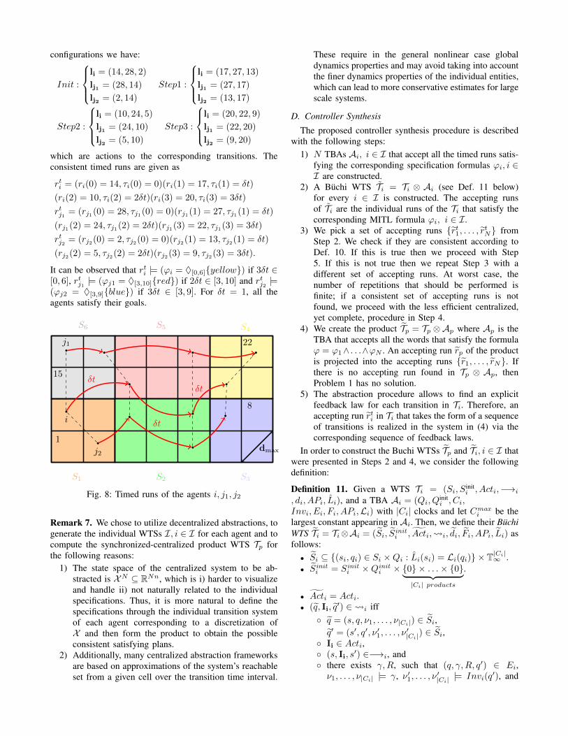
configurations we have:

Init :

li = (14, 28, 2)

lj1 = (28, 14)

lj2 = (2, 14)

Step1 :

li = (17, 27, 13)

lj1 = (27, 17)

lj2 = (13, 17)

Step2 :

li = (10, 24, 5)

lj1 = (24, 10)

lj2 = (5, 10)

Step3 :

li = (20, 22, 9)

lj1 = (22, 20)

lj2 = (9, 20)

which are actions to the corresponding transitions. Theconsistent timed runs are given as

rti = (ri(0) = 14, τi(0) = 0)(ri(1) = 17, τi(1) = δt)

(ri(2) = 10, τi(2) = 2δt)(ri(3) = 20, τi(3) = 3δt)

rtj1 = (rj1(0) = 28, τj1(0) = 0)(rj1(1) = 27, τj1(1) = δt)

(rj1(2) = 24, τj1(2) = 2δt)(rj1(3) = 22, τj1(3) = 3δt)

rtj2 = (rj2(0) = 2, τj2(0) = 0)(rj2(1) = 13, τj2(1) = δt)

(rj2(2) = 5, τj2(2) = 2δt)(rj2(3) = 9, τj2(3) = 3δt).

It can be observed that rti |= (ϕi = ♦[0,6]yellow) if 3δt ∈[0, 6], rtj1 |= (ϕj1 = ♦[3,10]red) if 2δt ∈ [3, 10] and rtj2 |=(ϕj2 = ♦[3,9]blue) if 3δt ∈ [3, 9]. For δt = 1, all theagents satisfy their goals.

i

j2

j1

dmax

22

8

15

1

S5 S4

S3S2S1

S6

δt

δt

δt

Fig. 8: Timed runs of the agents i, j1, j2

Remark 7. We chose to utilize decentralized abstractions, togenerate the individual WTSs I, i ∈ I for each agent and tocompute the synchronized-centralized product WTS Tp forthe following reasons:

1) The state space of the centralized system to be ab-stracted is XN ⊆ RNn, which is i) harder to visualizeand handle ii) not naturally related to the individualspecifications. Thus, it is more natural to define thespecifications through the individual transition systemof each agent corresponding to a discretization ofX and then form the product to obtain the possibleconsistent satisfying plans.

2) Additionally, many centralized abstraction frameworksare based on approximations of the system’s reachableset from a given cell over the transition time interval.

These require in the general nonlinear case globaldynamics properties and may avoid taking into accountthe finer dynamics properties of the individual entities,which can lead to more conservative estimates for largescale systems.

D. Controller Synthesis

The proposed controller synthesis procedure is describedwith the following steps:

1) N TBAs Ai, i ∈ I that accept all the timed runs satis-fying the corresponding specification formulas ϕi, i ∈I are constructed.

2) A Buchi WTS Ti = Ti ⊗ Ai (see Def. 11 below)for every i ∈ I is constructed. The accepting runsof Ti are the individual runs of the Ti that satisfy thecorresponding MITL formula ϕi, i ∈ I.

3) We pick a set of accepting runs rt1, . . . , rtN fromStep 2. We check if they are consistent according toDef. 10. If this is true then we proceed with Step5. If this is not true then we repeat Step 3 with adifferent set of accepting runs. At worst case, thenumber of repetitions that should be performed isfinite; if a consistent set of accepting runs is notfound, we proceed with the less efficient centralized,yet complete, procedure in Step 4.

4) We create the product Tp = Tp ⊗Ap where Ap is theTBA that accepts all the words that satisfy the formulaϕ = ϕ1∧ . . .∧ϕN . An accepting run rp of the productis projected into the accepting runs r1, . . . , rN. Ifthere is no accepting run found in Tp ⊗ Ap, thenProblem 1 has no solution.

5) The abstraction procedure allows to find an explicitfeedback law for each transition in Ti. Therefore, anaccepting run rti in Ti that takes the form of a sequenceof transitions is realized in the system in (4) via thecorresponding sequence of feedback laws.

In order to construct the Buchi WTSs Tp and Ti, i ∈ I thatwere presented in Steps 2 and 4, we consider the followingdefinition:

Definition 11. Given a WTS Ti = (Si, Siniti , Acti,−→i

, di, APi, Li), and a TBA Ai = (Qi, Qiniti , Ci,

Invi, Ei, Fi, APi,Li) with |Ci| clocks and let Cmaxi be the

largest constant appearing in Ai. Then, we define their BuchiWTS Ti = Ti⊗Ai = (Si, S

initi , Acti, i, di, Fi, APi, Li) as

follows:• Si ⊆ (si, qi) ∈ Si ×Qi : Li(si) = Li(qi) × T|Ci|∞ .• Sinit

i = Siniti ×Qinit

i × 0 × . . .× 0︸ ︷︷ ︸|Ci| products

.

• Acti = Acti.• (q, Ii, q

′) ∈ i iff q = (s, q, ν1, . . . , ν|Ci|) ∈ Si,q′ = (s′, q′, ν′1, . . . , ν

′|Ci|) ∈ Si,

Ii ∈ Acti, (s, Ii, s

′) ∈−→i, and there exists γ,R, such that (q, γ,R, q′) ∈ Ei,ν1, . . . , ν|Ci| |= γ, ν′1, . . . , ν

′|Ci| |= Invi(q

′), and

for all i ∈ 1, . . . , |Ci|

ν′i =

0, if ci ∈ Rνi + di(s, s

′), if ci 6∈ R andνi + di(s, s

′) ≤ Cmaxi

∞, otherwise.

Then, di(q, q′) = di(s, s′).

• Fi = (si, qi, ν1, . . . , ν|Ci|) ∈ Qi : qi ∈ Fi.• Li(si, qi, ν1, . . . , ν|Ci|) = Li(si).

The Buchi WTS Tp is constructed in a similar way. EachBuchi WTS Ti, i ∈ I is in fact a WTS with a Buchiacceptance condition Fi. A timed run of Ti can be writtenas rti = (qi(0), τi(0))(qi(1), τi(1)) . . . using the terminologyof Def. 5. It is accepting if qi(i) ∈ Fi for infinitely manyi ≥ 0. An accepting timed run of Ti projects onto a timedrun of Ti that satisfies the local specification formula ϕi byconstruction. Formally, the following lemma, whose prooffollows directly from the construction and and the principlesof automata-based LTL model checking (see, e.g., [45]),holds:

Lemma 2. Consider an accepting timed run rti =(qk(0), τi(0))(qi(1), τi(1)) . . . of the Buchi WTS Tk definedabove, where qi(k) = (ri(k), si(k), νi,1, . . . , νi,Mi) denotesa state of Ti, for all k ≥ 1. The timed run rti projectsonto the timed run rti = (ri(0), τi(0))(ri(1), τi(1)) . . .of the WTS Ti that produces the timed word w(rti) =(Li(ri(0)), τi(0))(Li(ri(1)), τi(1)) . . . accepted by the TBAAi via its run ρi = si(0)si(1) . . .. Vice versa, if thereexists a timed run rtk = (rk(0), τk(0))(rk(1), τk(1)) . . .of the WTS Tk that produces a timed word w(rtk) =(Lk(rk(0)), τi(0))(Li(ri(1)), τi(1)) . . . accepted by the TBAAi via its run ρi = si(0)si(1) . . . then there exist theaccepting timed run rti = (qi(0), τi(0))(qi(1), τi(1)) . . . ofTi, where qi(i) denotes (ri(k), si(k), νi,1(i), . . . , νi,Mi(k))

in Ti.

Proposition 1. By following the procedure described in Sec.IV-D a sequence of controllers v1, . . . , vN can be designed(if there is a solution according to Steps 1-5) that guaranteesthe satisfaction of the formulas ϕ1, . . . , ϕN of the agents1, . . . , N respectively, governed by dynamics as in (4).

E. Complexity

Our proposed framework can handle all the expressivity ofthe MITL formulas according to the semantics of Definition6. Denote by |ϕ| the length of an MITL formula ϕ. ATBA Ai, i ∈ I can be constructed in space and time2O(|ϕi)|, i ∈ I. So by denoting with ϕmax = max|ϕi, i ∈ Ithe MITL formula with the longest length we have thatthe complexity of Step 1 is 2O(|ϕmax)|. The model checkingof Step 2 costs O(|Ti| · 2|ϕi|), i ∈ I where |Ti| is thelength of the WTS Ti i.e., the number of its states. Thus,O(|Ti| · 2|ϕi|) = O(|Si| · 2|ϕi|) = O(|I| · 2|ϕi|). The worstcase of Step 2 costs O(|Tmax| · 2|ϕmax|) where |Tmax| is thenumber of the states of the WTS which corresponds to thelongest formula ϕmax. Due to the fact that all the WTSs in

Step 2 have the same number of states, it holds that the worstcase complexity of Step 2 costs O(|I| · 2|ϕmax|). By denotingwith Riter the finite number of repetitions of Step 3, we havethe best case complexity as O(Riter·|I|·2|ϕmax|), since the Step3 is more efficient than Step 4. The worst case complexity ofour proposed framework is when Step 4 is followed, whichis O(|I|N · 2|ϕmax|) where |I| is the number of cells of thecell decomposition S.

x axis-10 -5 0 5 10

yaxis

-10

-8

-6

-4

-2

0

2

4

6

8

10

Agent 1

Agent 2

Agent 3

Set X

Goal Ag.1

Goal Ag.2

Goal Ag.3

Fig. 9: Space discretization, goal regions and reachable setsfor each agent in a time horizon of 11δt steps

V. SIMULATION RESULTS

For a simulation example, a system of three agents withxi ∈ R2, i ∈ I = 1, 2, 3, E = 1, 2, 2, 3,N (1) =2 = N (3),N (2) = 1, 3 is considered. Their dynamicsare given as x1 = x2 − x1 + v1, x2 = x1 + x3 − 2x2 + v2

and x3 = x2 − x3 + v3. The simulation parameters are setto R = 10,M = 20, vmax = 10, L1 =

√2, L2 = 2, δt = 0.2.

The time step δt is chosen during the abstraction processaccording to the formulas (21), (22) and it is not chosenwith reference to satisfaction of the MITL formulas. Theworkspace [−10, 10] × [−10, 10] ⊆ R2 is partitioned intocells and the initial agents’ positions are set to (−6, 0), (0, 6)and (6, 0) respectively. The specification formulas are setto ϕ1 = ♦[0.5,1.7]green, ϕ2 = ♦[1.0,1.4]orange, ϕ3 =♦[0.7,1.8]black respectively and their corresponding TBAsare given in Fig. 3. The abstraction presented in this pa-per, the reachable cells of each agent as well as the goalregions are depicted in Fig. 9. It can be observed that notall the individual runs satisfy the desired specification. Byapplying the five-step controller synthesis procedure that waspresented in Sec. IV, the individual run of each agent satisfythe formulas ϕ1, ϕ2 and ϕ3 in 6δt, 6δt and 5δt respectively.The simulation is performed in a horizon of 11δt steps (asthe steps that explained in the Example 6). The product WTS

has 45 × 104 states. The simulations were carried out inMATLAB Environment on a desktop with 8 cores, 3.60GHzCPU and 16GB of RAM.

VI. CONCLUSIONS AND FUTURE WORK

A systematic method of both abstraction and controllersynthesis of dynamically coupled multi-agent path-planninghas been proposed, in which timed constraints of fulfillinga high-level specification are imposed to the system. Thesolution involves initially a boundedness analysis and sec-ondly the abstraction of each agent’s motion into WTSs andautomata construction. The simulation example demonstratesour solution approach. Future work includes further compu-tational improvement of the abstraction method and morecomplicated high-level tasks being imposed to the agents inorder to exploit the expressiveness of MITL formulas.

REFERENCES

[1] W. Ren and R. Beard, “Consensus Seeking in Multi-Agent SystemsUnder Dynamically Changing Interaction Topologies,” IEEE Transac-tions on Automatic Control, vol. 50, no. 5, pp. 655–661, 2005.

[2] R. Olfati-Saber and R. Murray, “Consensus Problems in Networks ofAgents with Switching Topology and Time-Delays,” IEEE Transac-tions on Automatic Control, vol. 49, no. 9, pp. 1520–1533, 2004.

[3] A. Jadbabaie, J. Lin, and S. Morse, “Coordination of Groups ofMobile Autonomous Agents Using Nearest Neighbor Rules,” IEEETransactions on Automatic Control, vol. 48, no. 6, pp. 988–1001, 2003.

[4] G. Shi and K. Johansson, “Robust Consensus for Continuous-TimeMulti-Agent Dynamics,” SIAM Journal on Control and Optimization,vol. 51, no. 5, pp. 3673–3691, 2013.

[5] H. Tanner, A. Jadbabaie, and G. Pappas, “Flocking in Fixed andSwitching Networks,” IEEE Transactions on Automatic Control,vol. 52, no. 5, pp. 863–868, 2007.

[6] M. Egerstedt and X. Hu, “Formation Constrained Multi-Agent Con-trol,” IEEE Transactions on Robotics and Automation, vol. 17, no. 6,pp. 947–951, 2001.

[7] M. Zavlanos and G. Pappas, “Distributed Connectivity Control ofMobile Networks,” IEEE Transactions on Robotics, vol. 24, no. 6,pp. 1416–1428, 2008.

[8] S. Loizou and K. Kyriakopoulos, “Automatic Synthesis of Multi-AgentMotion Tasks Based on LTL Specifications,” 43rd IEEE Conferenceon Decision and Control (CDC 2004), vol. 1, pp. 153–158, 2004.

[9] M. Guo and D. Dimarogonas, “Multi-Agent Plan Reconfiguration Un-der Local LTL Specifications,” The International Journal of RoboticsResearch, vol. 34, no. 2, pp. 218–235, 2015.

[10] S. Karaman and E. Frazzoli, “Linear Temporal Logic Vehicle Routingwith Applications to Multi-UAV Mission Planning,” InternationalJournal of Robust and Nonlinear Control, vol. 21, no. 12, pp. 1372–1395, 2011.

[11] Y. Chen, Ding, X. Chu, A. Stefanescu, and C. Belta, “Formal Approachto the Deployment of Distributed Robotic Teams,” IEEE Transactionson Robotics, vol. 28, no. 1, pp. 158–171, 2012.

[12] M. Kloetzer, X. C. Ding, and C. Belta, “Multi-Robot Deploymentfrom LTL Specifications with Reduced Communication,” 50th IEEEConference on Decision and Control (CDC 2011), pp. 4867–4872,2011.

[13] H. Kress-Gazit, G. Fainekos, and G. Pappas, “Temporal-Logic-Based Reactive Mission and Motion Planning,” IEEE Transactionson Robotics, vol. 25, no. 6, pp. 1370–1381, 2009.

[14] A. Ulusoy, S. Smith, X. Ding, C. Belta, and D. Rus, “Optimalityand Robustness in Multi-Robot Path Planning with Temporal LogicConstraints,” The International Journal of Robotics Research, vol. 32,no. 8, pp. 889–911, 2013.

[15] M. Quottrup, T. Bak, and R. Zamanabadi, “Multi-Robot Planning:A Timed Automata Approach,” IEEE International Conference onRobotics and Automation (ICRA 2004), vol. 5, pp. 4417–4422, 2004.

[16] A. Ulusoy, S. Smith, X. Ding, C. Belta, and D. Rus, “Optimal Multi- Robot Path Planning with Temporal Logic Constraints,” IEEE/RSJInternational Conference on Intelligent Robots and Systems (IROS2011), pp. 3087–3092, 2011.

[17] J. Liu and P. Prabhakar, “Switching Control of Dynamical Systemsfrom Metric Temporal Logic Specifications,” IEEE International Con-ference on Robotics and Automation (ICRA 2014), pp. 5333–5338,2014.

[18] V. Raman, A. Donze, D. Sadigh, R. Murray, and S. Seshia, “ReactiveSynthesis from Signal Temporal Logic Specifications,” 18th Inter-national Conference on Hybrid Systems: Computation and Control(HSCC 2015), pp. 239–248, 2015.

[19] Y. Zhou, D. Maity, and J. S. Baras, “Timed Automata Approach forMotion Planning Using Metric Interval Temporal Logic,” EuropeanControl Conference (ECC 2016), 2016.

[20] J. Fu and U. Topcu, “Computational Methods for Stochastic Controlwith Metric Interval Temporal Logic Specifications,” 54th IEEE Con-ference on Decision and Control (CDC 2015), pp. 7440–7447, 2015.

[21] B. Hoxha and G. Fainekos, “Planning in Dynamic EnvironmentsThrough Temporal Logic Monitoring,” 2016.

[22] S. Karaman and E. Frazzoli, “Vehicle Routing Problem with MetricTemporal Logic Specifications,” 47th IEEE Conference on Decisionand Control (CDC 2008), pp. 3953–3958, 2008.

[23] A. Nikou, J. Tumova, and D. Dimarogonas, “Cooperative Task Plan-ning of Multi-Agent Systems Under Timed Temporal Specifications,”American Control Conference (ACC 2016), pp. 13–19, 2016.

[24] R. Alur, T. Henzinger, G. Lafferriere, and G. Pappas, “DiscreteAbstractions of Hybrid Systems,” Proceedings of the IEEE, vol. 88,no. 7, pp. 971–984, 2000.

[25] M. Zamani, G. Pola, M. Mazo, and P. Tabuada, “Symbolic Modelsfor Nonlinear Control Systems without Stability Assumptions,” IEEETransactions on Automatic Control, vol. 57, no. 7, 2012.

[26] E. A. Gol and C. Belta, “Time-Constrained Temporal Logic Controlof Multi-Affine Systems,” Nonlinear Analysis: Hybrid Systems, 2013.

[27] J. Liu and N. Ozay, “Finite Abstractions With Robustness Marginsfor Temporal Logic-Based Control Synthesis,” Nonlinear Analysis:Hybrid Systems, vol. 22, pp. 1–15, 2016.

[28] M. Zamani, M. Mazo, and A. Abate, “Finite Abstractions of Net-worked Control Systems,” 53rd IEEE Conference on Decision andControl (CDC 2014), pp. 95–100, 2014.

[29] M. Rungger and M. Zamani, “Compositional Construction of Approxi-mate Abstractions,” 18th International Conference on Hybrid Systems:Computation and Control (HSCC 2015), pp. 68–77, 2015.

[30] E. Dallal and P. Tabuada, “On Compositional Symbolic ControllerSynthesis Inspired by Small-Gain Theorems,” 54th IEEE Conferenceon Decision and Control (CDC), pp. 6133–6138, 2015.

[31] G. Pola, P. Pepe, and M. D. D. Benedetto, “Symbolic Models forNetworks of Control Systems,” IEEE Transactions on AutomaticControl, 2016.

[32] D. Boskos and D. Dimarogonas, “Decentralized Abstractions ForMulti-Agent Systems Under Coupled Constraints,” 54th IEEE Con-ference on Decision and Control (CDC 2015), pp. 282–287, 2015.

[33] M. Mesbahi and M. Egerstedt, “Graph Theoretic Methods in Multia-gent Networks,” 2010.

[34] R. Alur and D. Dill, “A Theory of Timed Automata,” TheoreticalComputer Science, vol. 126, no. 2, pp. 183–235, 1994.

[35] D. D. Souza and P. Prabhakar, “On the Expressiveness of MTL inthe Pointwise and Continuous Semantics,” International Journal onSoftware Tools for Technology Transfer, vol. 9, no. 1, pp. 1–4, 2007.

[36] J. Ouaknine and J. Worrell, “On the Decidability of Metric TemporalLogic,” 20th Annual IEEE Symposium on Logic in Computer Science(LICS’05), pp. 188–197, 2005.

[37] R. Alur, T. Feder, and T. A. Henzinger, “The Benefits of RelaxingPunctuality,” Journal of the ACM (JACM), vol. 43, no. 1, pp. 116–146, 1996.

[38] M. Reynolds, “Metric Temporal Logics and Deterministic TimedAutomata,” 2010.

[39] P. Bouyer, “From Qualitative to Quantitative Analysis of TimedSystems,” Memoire dhabilitation, Universite Paris, vol. 7, pp. 135–175, 2009.

[40] S. Tripakis, “Checking Timed Buchi Automata Emptiness on Simu-lation Graphs,” ACM Transactions on Computational Logic (TOCL),vol. 10, no. 3, 2009.

[41] O. Maler, D. Nickovic, and A. Pnueli, “From MITL to Timed Au-tomata,” International Conference on Formal Modeling and Analysisof Timed Systems, pp. 274–289, 2006.

[42] D. Nickovic and N. Piterman, “From MTL to Deterministic TimedAutomata,” Formal Modeling and Analysis of Timed Systems, 2010.

[43] D. Boskos and D. Dimarogonas, “Robust Connectivity Analysis forMulti-Agent Systems,” 54th IEEE Conference on Decision and Con-trol (CDC 2015), pp. 6767–6772, 2015.

[44] M. M. Fiedler, “Algebraic Connectivity of Graphs,” CzechoslovakMathematical Journal, vol. 23, no. 2, pp. 298–305, 1973.

[45] C. Baier, J. Katoen, and K. G. Larsen, Principles of Model Checking.MIT Press, 2008.