Cooperation versus Dominance

Hierarchies in Animal Groups

Jasvir Kaur Grewal

Oriel College

University of Oxford

A thesis submitted for the degree of

MSc in Mathematical Modelling and Scientific Computing

September 2012

Acknowledgements

Firstly, I would like to thank my three amazing supervisors – Marian

Dawkins, Cameron Hall, and Mason Porter – for their invaluable help

and guidance during the writing of this dissertation. I doubt that I would

have enjoyed this project as much as if I have done it without them. Also,

I would like to thank Kathryn Gillow for her help over the year. Most

importantly, I would like to thank my family for their endless support.

Abstract

While some communities of animals living in groups may develop systems

of cooperation or mutual altruism, many other animal societies are charac-

terised by dominance hierarchies. This thesis is concerned with describing

the development of cooperation and dominance hierarchies amongst ani-

mal groups.

By using a game-theoretic framework, I develop and investigate simple

models to describe social interactions amongst animals. In particular, I

consider the situation in which the animals differ from each other by some

asymmetry and I analyse the effect of such individual differences on the

models.

Unlike earlier work in this field, which tended to focus on cooperation

or dominance hierarchies in isolation, I develop a model that allows both

cooperation and dominance hierarchies to arise. Additionally, this work

is novel in that it makes a connection between the Hawk–Dove model and

the formation of a dominance hierarchy.

I begin my analysis with a static analysis of the asymmetric Hawk–Dove

game, using the concept of an evolutionary stable strategy. This is fol-

lowed by the application of replicator dynamics to the problem. My anal-

ysis shows that neither of these standard approaches allow cooperation as

an outcome, which motivates me to develop new but tractable dynamic

models.

The final model presented allows both cooperation and dominance re-

lations in different circumstances, and I discuss how it can be used to

model the formation of a dominance hierarchy. Finally, I investigate how

much asymmetry is required in order to make qualitative differences in

the relative frequencies of cooperation and dominance hierarchies.

Contents

1 Introduction 1

2 Background Material 4

2.1 Classical Game Theory . . . . . . . . . . . . . . . . . . . . . . . . . . 4

2.2 Zoological Background . . . . . . . . . . . . . . . . . . . . . . . . . . 7

2.3 Evolutionary Game Theory . . . . . . . . . . . . . . . . . . . . . . . 8

3 Modelling the Problem 12

4 Two Standard Approaches 17

4.1 Static Analysis . . . . . . . . . . . . . . . . . . . . . . . . . . . . . . 17

4.2 Dynamic Analysis . . . . . . . . . . . . . . . . . . . . . . . . . . . . . 20

5 Incorporating Strategy Updates 25

5.1 Simulations . . . . . . . . . . . . . . . . . . . . . . . . . . . . . . . . 27

5.2 Dominance of a Smaller Animal . . . . . . . . . . . . . . . . . . . . . 30

5.3 Limitations of the Model . . . . . . . . . . . . . . . . . . . . . . . . . 31

5.4 Modification of the Model . . . . . . . . . . . . . . . . . . . . . . . . 32

6 Incorporating Uncertainty 34

6.1 Updating the Asymmetry Estimates . . . . . . . . . . . . . . . . . . . 35

6.2 Simulations . . . . . . . . . . . . . . . . . . . . . . . . . . . . . . . . 36

6.3 Bayesian Updating . . . . . . . . . . . . . . . . . . . . . . . . . . . . 39

7 Hierarchy Formation 42

7.1 Calculating the Hierarchy Order . . . . . . . . . . . . . . . . . . . . . 42

i

8 Discussion 46

9 Conclusion 49

Appendix 51

Bibliography 53

ii

Chapter 1

Introduction

Examples of animals living in groups are seen frequently in nature. The benefits that

animals gain by living together include the dilution of predation risk and increased

foraging success [7]. However, the limited availability of resources such as water,

food, and space implies that members of animal groups must formulate methods with

which to divide the restricted resources amongst themselves. This will often result in

animals competing with other group members over the limited resources.

In such situations, animals need to decide what type of behaviour to exhibit

when interacting with their competitors. Research in ethology, the study of animal

behaviour, has shown that there are various types of behaviour that animals routinely

exhibit when in the situation of competing for a resource. As explained in [55],

competing animals sometimes first exchange ‘displays’ of strength, which involve little

energy consumption or injury risk and hence are of relatively low cost to the animal.

Then, if no animal withdraws from the competition, there is an escalation in behaviour

and the animals become more aggressive. The animal who wins a fight (which occurs

after both animals escalate) or whose opponent has withdrawn wins the resource.

The allocation of resources will have a significant effect on each animal’s fitness,

and in particular, their Darwinian fitness. Broadly speaking, Darwinian fitness refers

to an animal’s survival and reproductive success [28]. In situations of limited re-

sources, there will be a ‘survival of the fittest’ scenario in which the more successful

traits (or phenotypes) will be passed onto offspring.

In this thesis, I aim to make a contribution to the understanding of two contrast-

ing styles of animal interaction: cooperation and dominance hierarchies. Cooperation

refers to situations where animals voluntarily share resources. Interestingly, research

has shown that cooperation between members of animal groups occurs in many differ-

ent types of species, ranging from honeybees [67] to vervet monkeys [63]. For example,

vampire bats have been observed to regurgitate blood that they have obtained in or-

der to give it to a hungry member of their colony [73]. However, cooperation seems

1

paradoxical when considering Darwin’s theory of ‘survival of the fittest’. Surely an

animal that cooperates with its opponents lowers its own Darwinian fitness?

One alternative to cooperation is dominance hierarchies, where the dominant in-

dividuals obtain a larger share of the resources than inferior individuals. These occur

commonly in animal groups and examples of such social structures include dominance

hierarchies observed in crayfish [44] or pecking orders in flocks of chickens [33]. Ani-

mals benefit from being members of stable dominance hierarchies due to the reduction

in the number of costly fights. Fighting carries a risk of injury as well as energetic

costs, so it is preferable for animals to avoid fighting [58]. Additionally, there are

situations (such as being in the presence of a predator) in which animals are better

off being part of a dominance hierarchy than being alone [43].

Many of the aforementioned studies of animal behaviour have noted regular fea-

tures observed in the formation of dominance hierarchies. First, there are often high

levels of aggression amongst animals when they are first brought together to form a

group. Additionally, the levels of aggression tend to drop as the experiment progresses

– for instance, in [44], the levels of fighting had reduced significantly within a hour of

the experiment. In this thesis, I explore how cooperation and dominance hierarchies

can both result from repeated interactions between members of animal groups.

The members of animal groups vary by characteristics such as age, gender, and

size, so it is also important to incorporate individual asymmetries in models. For

convenience, I consider only one asymmetry – the size difference between animals. I

choose to consider this asymmetry over other possible alternatives because research

suggests that it is a key factor in animal contests over a large range of different

species [27, 53, 72]. As explained in [1] and [50], larger animals usually win escalated

contests, and hence relative body-size is one of the most important determinants of

the outcome of a fight.

One would expect that changing the degree of asymmetry would also change the

relative frequencies of cooperation versus dominance hierarchies – an animal that

is much larger than its opponent (and hence more likely to win in a fight) will be

aggressive more frequently than a smaller animal [13]. In my analysis, I examine

the effect of varying the asymmetry on the relative frequencies of cooperation versus

dominance hierarchies.

The aim of this thesis is to derive a model that accounts for the individual asymme-

tries of animals and allows both cooperation and dominance hierarchies as outcomes

2

in different circumstances. Since there are various different strategies that can be

used when animals conflict over resources, my aim is to explain the circumstances in

which each strategy may be adopted. The standard approach to such evolutionary

problems is to use game theory, which provides a convenient framework in which to

analyse the different behaviours that animals can display.

In Chapter 2, I briefly outline background material from game theory, focussing

on evolutionary game theory. I also survey some of the recent research that in rel-

evant to the development of models of cooperation and dominance hierarchies. In

Chapter 3, I formulate the problem of competition for resources amongst asymmetric

individuals in the language of game theory. Standard approaches to analysing evolu-

tionary games include static and dynamic analyses, which are described in Chapter 4.

However, I will show that the desired result cannot be reached using these standard

techniques. Hence, I develop and create novel simple models to investigate the exis-

tence of cooperation and dominance hierarchies in Chapters 5 and 6. In Chapter 7, I

then consider how the results of such models can be used to model the formation of a

dominance hierarchy. Chapter 8 contains a discussion of results, and then I conclude

and suggest possible extensions to this work in Chapter 9.

3

Chapter 2

Background Material

2.1 Classical Game Theory

Consider a situation with two or more entities who must decide how to strategically

interact with each other in the setting of a ‘game’ with set outcomes and strategies.

The study of such strategic interactions is called game theory. Game theory is often

used in the setting of ethology [6, 38, 75], as game theory can translate a complex ani-

mal conflict situation into a convenient mathematical format where optimal solutions,

if they exist, can be determined.

Game theory has been applied in a wide variety of settings including economics

[26], politics [10], computer science [36], and football [22]. Its wide applicability

to many decision-making processes and the way in which it can simplify seemingly

complex problems into a form (called a ‘game’) that is much easier to analyse makes

game theory very useful.

A well-known example of such a game is referred to as the ‘prisoner’s dilemma’

[4]. Imagine a pair of friends (A and B) who have been arrested over some crime

and now must separately make the decision of whether to confess (‘defect’ from each

other) or not confess (‘cooperate’ with each other). For the purpose of the game, I

also assume that they have no way of communicating with each other.

Each individual is offered the same deal by the police: if one of the pair confesses

that the pair committed the crime, whilst the other remains silent, then the confessor

will get a significantly reduced prison sentence of 1 year and the other individual will

get a sentence of 10 years. In the case that both friends confess, each will receive a

prison sentence of 8 years; in the case that both do not confess, each will receive a

sentence of 4 years.

In the standard language of game theory, the two people are called the ‘players’

of the game, the decisions that the players can make are called ‘strategies’, and the

4

rewards that players can receive are called ‘payoffs’ (which are negative in the case

of prison sentences).

Using a game-theoretic model of this scenario, an individual can strategically

analyse which decision should be made. Game theory makes the assumption that

each player is perfectly rational and selfish (that is, each tries to maximise his/her

payoff). The different cases of the situation can be modelled succinctly using the

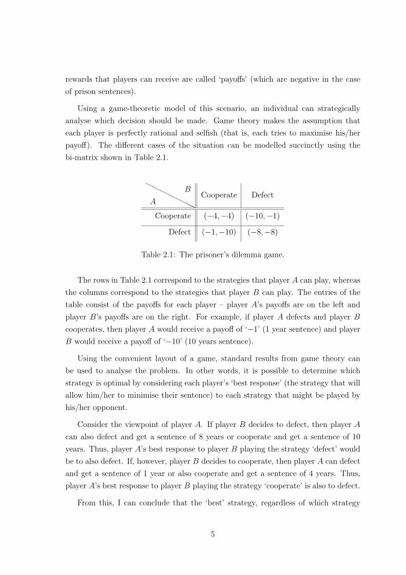
bi-matrix shown in Table 2.1.

HHHHHH

HHA

BCooperate Defect

Cooperate (−4,−4) (−10,−1)

Defect (−1,−10) (−8,−8)

Table 2.1: The prisoner’s dilemma game.

The rows in Table 2.1 correspond to the strategies that player A can play, whereas

the columns correspond to the strategies that player B can play. The entries of the

table consist of the payoffs for each player – player A’s payoffs are on the left and

player B’s payoffs are on the right. For example, if player A defects and player B

cooperates, then player A would receive a payoff of ‘−1’ (1 year sentence) and player

B would receive a payoff of ‘−10’ (10 years sentence).

Using the convenient layout of a game, standard results from game theory can

be used to analyse the problem. In other words, it is possible to determine which

strategy is optimal by considering each player’s ‘best response’ (the strategy that will

allow him/her to minimise their sentence) to each strategy that might be played by

his/her opponent.

Consider the viewpoint of player A. If player B decides to defect, then player A

can also defect and get a sentence of 8 years or cooperate and get a sentence of 10

years. Thus, player A’s best response to player B playing the strategy ‘defect’ would

be to also defect. If, however, player B decides to cooperate, then player A can defect

and get a sentence of 1 year or also cooperate and get a sentence of 4 years. Thus,

player A’s best response to player B playing the strategy ‘cooperate’ is also to defect.

From this, I can conclude that the ‘best’ strategy, regardless of which strategy

5

the opponent might play is to defect.1 However, both individuals are assumed to

be perfectly rational and selfish, so any players’ opponent will also decide that the

best strategy to play is to defect. This is the interesting feature of the prisoner’s

dilemma. Both players decide to play their ‘best’ strategy of defect, which will lead

to an outcome where each serves a longer sentence than if they had both cooperated.

However, a small amendment of the one-round prisoner’s dilemma scenario above

gives interesting results. Now consider the case of an iterated prisoner’s dilemma,

where the game is played by the same two players more than once. This fundamentally

changes the outcome because players can use the information obtained from previous

rounds to help them decide which strategy to play.

Interestingly, when considering an iterated prisoner’s dilemma, cooperation can

occur. Because a player will know the strategies that its opponent has played pre-

viously, defecting will cause more harm, as this will encourage its opponent to also

defect in future rounds. Thus, both might cooperate and this will earn them signifi-

cantly better payoffs than any other strategy would over the N rounds of the game.

Note, importantly, that I assume the number of rounds, N , of the prisoner’s dilemma

to be played is unknown to both players. If N were known, backwards induction

implies that defecting would still be the optimal strategy [4].

Thus, cooperation can exist as an optimal strategy in the iterated prisoner’s

dilemma, even if defection is always optimal in a one-off encounter. A famous exam-

ple of this is the ‘tit for tat’ strategy [4], which was discovered during a computer

tournament for a winning strategy of the iterated prisoner’s dilemma. An individual

that plays the tit for tat strategy cooperates in the first round of the game; in further

rounds the player simply copies the strategy that was last employed by its opponent.

This example is important because it highlights how considering repeated inter-

actions (which would certainly be the case in a group of animals) might lead to coop-

eration. Additionally, behaviour similar to the tit for tat strategy has been observed

in a variety of different species (see, for example, [30] and [47]).

1Using standard game-theory terminology, the set of strategies in which both players play their

optimal strategy and the corresponding payoffs is a ‘Nash equilibrium’.

6

2.2 Zoological Background

The paradoxical nature of resource-sharing (an animal that shares the resource is

lowering its Darwinian fitness) makes it a popular subject within biology. This has

led to the development of a variety of theories on how and when resource-sharing

occurs amongst animals. While a comprehensive review is beyond the scope of this

thesis, I will motivate my use of game theory and related models by describing some

of the broad themes in current research on resource-sharing.

First, a lot of research has been carried out to find the reasons why cooperation ac-

tually occurs in practice. Studies investigating the occurrence of cooperation between

animals have suggested four main explanations: reciprocity, by-product mutualism,

kin selection, and group selection [24].

Reciprocity is what can be seen in the prisoner’s dilemma - cooperation occurs

with the hope that an opponent will also cooperate in the future. By-product mu-

tualism refers to cooperation occurring when an animal, whilst benefiting itself, also

unintentionally benefits its opponent. Kin selection is cooperation due to the animals

being related. Finally, group selection explains that cooperation occurs for the good

of the group [24].

Various approaches have been developed to model cooperation. I have already

discussed how a game-theoretic approach can be used to model the evolution of co-

operation – a ‘tit for tat’ strategy can lead to cooperation in the iterated prisoner’s

dilemma. However, such a model has limited use, because cooperation will only be

reached if the competitors start by cooperating. As discussed earlier, when animals

first meet, there are usually high levels of aggression, so starting with a cooperative

strategy would be an unreasonable feature to include in my model.

Dominance hierarchies play an significant role in phenotypic evolution because

more dominant animals have greater access to important resources than subordinate

members of an animal group. The hierarchies can be classified as being egalitarian

(benefits are equally shared between the animals) or despotic (animals higher in the

hierarchy receive more benefits than those lower) [70].

Many models have also been developed for the formation of a dominance hierarchy

in animal groups (see, for example, [12] and [54]). Unlike earlier work in this field,

which tended to focus on cooperation or dominance hierarchies in isolation, I seek a

model that allows both cooperation and dominance hierarchies to arise.

7

It is interesting to note that there are two phases of hierarchy development – a

formation phase (when a group of animals meets for the first time), and a maintenance

phase (when the hierarchy has been formed but there may be changes for reasons such

as the introduction of a new animal). When constructing a model for a dominance

hierarchy, it is important to create a model that incorporates both phases of the

hierarchy development in what Broom refers to as a ‘unified’ model [12].

The discussion of a maintenance phase also highlights another important feature –

dominance hierarchies are not permanent and might change over time [48]. Another

interesting aspect of animal behaviour is that, although rare, some species display

female dominance, where every adult female dominates every adult male [56]. Addi-

tionally, research has shown that lower ranking animals may form alliances in order

to gain a competitive advantage against other animals [15].

The aim of this thesis is to develop a simple model for the formation of dominance

hierarchies and the occurrence of cooperation in animal groups. In this section, I have

listed some characteristics of animal behaviour. Although the model which I develop

in this thesis will not show all of these different observations, the discussion provides

motivation for a number of interesting possible extensions. I will tackle my problem

within the framework of evolutionary game theory, which I discuss in the next section.

2.3 Evolutionary Game Theory

I want to model how the interactions between animals living in groups can result in

cooperation and dominance hierarchies. Earlier, I explained that game theory can

be used to model the strategic interactions between ‘players’. In particular, I work

within the field of evolutionary game theory, which studies the strategic interactions

between members of evolving populations of organisms such as animals or plants.

Although evolutionary game theory has now been studied for several decades, even

the classical theory is still able to provide new and exciting insights [3]. Evolutionary

game theory is motivated by the expectation that more successful strategies will

prevail over time, as compared to strategies that give lower payoffs. The evolutionary

equivalent of the classical game theory assumption that players are rational is that

survival of the fittest will lead towards players optimising their reproductive success

[37].

8

A common criticism of evolutionary game theory involves questioning how the

players of such evolutionary games (in my case, animals) can be reasonably expected

to make rational decisions for themselves. However, as Maynard Smith explained in

[64], evolutionary game theory does not rely on the assumption that animals try to

maximise their payoffs. Rather, the optimisation of the game-theoretic model can

provide a way of determining the result that nature would obtain.

It is important to note that there are a few key differences between game theory

and evolutionary game theory. Most importantly, the players in an evolutionary game

do not make conscious decisions unlike in classical game theory. Instead, the players

inherit their behaviour from their forebears [52].

Additionally, recall the prisoner’s dilemma example from Section 2.1 and remem-

ber that the payoffs in the matrix corresponded to the jail sentences that each player

would have to serve. In the context of evolutionary game theory, the payoffs in an

evolutionary game will now represent changes in Darwinian fitness. In this way, a

strategy can be measured relative to other strategies to see how much it can benefit

an animal’s reproductive success.

By providing an alternative way in which to model the evolution of a population,

evolutionary game theory has led to some significant advances in the study of animal

behaviour [35]. In the 1970s, Maynard Smith created a framework in which to model

animal conflicts. He formulated the ‘Hawk–Dove’ game, which models the situation

in which two animals are contesting over some resource of value V and any injury

obtained will cause a decrease in Darwinian fitness by an amount C.

Maynard Smith assumed that animals can behave in one of two ways – like a

‘Dove’ or like a ‘Hawk’ [64]. An animal that behaves like a Dove first displays but

then retreats at once if its opponent escalates. An animal that behaves like a Hawk

always escalates and continues until it is injured or its opponent retreats.

If both animals behave like Doves, then they each gain an equal share of the

resource. If one animal behaves like a Dove, whilst the other behaves like a Hawk,

then whichever animal is playing the Hawk strategy wins the whole resource. Note

that in this case, there is a dominance relation. As explained in [16], a dominance

relation exists between two individuals when one attacks or threatens to attack the

other, whereas the other shows little or no aggression. Finally, in the case in which

both animals play the Hawk strategy, there will be a fight. Maynard Smith assumed

that in this situation each animal has 50% chance of injury and 50% chance of winning

9

the fight (by injuring its opponent). Hence, the expected payoff that each animal

would receive in the Hawk–Hawk case would be V−C2

.

Similar to how the prisoner’s dilemma was summarised into a game matrix, the

corresponding game for the Hawk–Dove model is given in Table 2.2.

HHHHH

HHHA

BDove Hawk

Dove

(V

2,V

2

)(0,V )

Hawk (V ,0)

(V − C

2,V − C

2

)Table 2.2: The Hawk–Dove game.

Maynard Smith also introduced a concept with which to analyse such an evolu-

tionary game, similar to how the prisoner’s dilemma example could be analysed for

Nash equilibria. He introduced the term ‘evolutionary stable strategy’, which is a

strategy such that if all members of a population adopted the strategy, then a mu-

tant strategy could not invade the population. In other words, no mutant strategy

can prevail when all animals in the group adopt the evolutionary stable strategy.

I will use the Hawk–Dove model as a foundation for my work. My problem

is different in that I do not assume that each animal has an equal probability of

winning a fight as I want to account for asymmetries in animal groups. Instead of the

symmetric game shown in Table 2.2, my problem will correspond to an asymmetric

game, which I will present in Chapter 3. Thus, I need to consider a slightly modified

definition for an evolutionary stable strategy that describes a strategy for each player.

I use similar notation to that in [64], where πi(X, Y ) is the payoff to animal i

when animal A plays strategy X and animal B plays strategy Y .

Definition: A strategy pair (I∗, J∗) is called an evolutionary stable strategy (ESS) if

πA(I∗, J) > πA(I, J) for all I 6= I∗

and

πB(I, J∗) > πB(I, J) for all J 6= J∗.

10

Essentially, each strategy in the pair has to give a strictly better payoff than what

would be achieved by using another available strategy [2]. Note that an evolutionary

stable strategy does not guarantee that a population will tend to that strategy. The

definition of an evolutionary stable strategy requires the majority of a population to

be playing that strategy, and such a strategy could be ‘inaccessible’ [51]. Nevertheless,

it is still a useful concept as it can provide insight into the possible evolutionary states

that a population can obtain.

In my problem, I can use evolutionary game theory to understand how the strate-

gies played by members of animal groups ‘evolve’ over time. By considering which

behaviours survive the process of ‘natural selection’, I then should be able to deter-

mine whether cooperation or dominance hierarchies result.

I differ from existing work in the field by the way in which I will make a connection

between the Hawk–Dove model and the formation of a dominance hierarchy. In the

next chapter, using the Hawk–Dove model, I will show that an appropriate idealisation

of animals interactions can be expressed as an asymmetric game.

Additionally, one can analyse games through the use of ordinary differential equa-

tions [40]. One of the most popular methods used to investigate evolutionary games

is the replicator dynamics model [68, 71], which studies how the frequencies of each

possible strategy evolve, assuming that an animal passes on its ‘behaviour type’ to

its offspring. I study replicator dynamics in further detail in Chapter 4.

Here, I note an important result related to my problem involving ‘mixed’ evolu-

tionary stable strategies. A pure evolutionary stable strategy pair for an asymmetric

game is an ESS in which each player adopts only one strategy throughout its lifetime.

A mixed ESS can be achieved in one of two ways. The first way is by having players

adopting strategies at random. The second way is by interpreting each player to be

a population of players (who play the same strategy during their lifetimes) in which

more than one type of strategist exist.

When considering symmetric games, in which one can switch players A and B

without changing the problem, it is often the case that there exist ‘mixed’ evolutionary

stable strategies. However, Selten proved in 1980 that asymmetric games have no

mixed ESSs [62]. Selten showed that any ESS of asymmetric animal conflicts can

only consist of pure strategies if the animals know the size of the asymmetry [64].

This is useful because it reduces the number of possible points in the strategy space

that need to be examined for ESSs.

11

Chapter 3

Modelling the Problem

I outline the assumptions that I shall make in the modelling of the problem. I follow

the assumptions made by Maynard Smith in [64]. However, because the problem

that I am considering differs from Maynard Smith’s classical Hawk–Dove model by

the introduction of an asymmetry, I will also need a further simplifying assumption

(Assumption 2).

Assumptions:

1. There is a limited amount of the resource that is being contested.

Dominance becomes an important concept only when the resource for which

competitors are competing is limited [32, 44]. Thus, I make this assumption so

that dominance hierarchies can actually form.

2. The sizes of the animals in the group are fixed.

Although, this might seem at first to be an unreasonable assumption, research

suggests that a change in the body-size of animals need not have a significant

effect on animal behaviour. For example, Abbot, Dunbrack, and Orr, whilst

conducting experiments with fish, found that even when subordinate fish later

became up to 50% larger than the dominant fish, they still did not contest the

order [1]. The authors suggested that the risk of injury and the low probability of

the size differences changing meant that the fish concerned used the experience

of previous encounters to settle contests rather than fighting. As I will show in

Chapter 5, the more advanced models in this thesis have the property that a

stable dominance relation can develop where the weaker individual is dominant.

3. There is only asexual reproduction.

This assumption is usually made in evolutionary game theory so that the evo-

lution of strategies can be analysed easily. Since animals are assumed to pass

12

on their behaviour onto their offspring, the assumption of asexual reproduction

means that the success of different behaviour types can be tracked easily.

4. The resource is divisible.

I assume this so that cooperation (in the form of sharing the resource) can occur.

Discussion concerning games over indivisible resources can be found in [64].

In such cases, if both animals play the Dove strategy, then whichever animal

‘displays’ the longest wins the resource. Also, concepts such as displaying costs

(which I do not consider in this thesis) become more important when examining

games over indivisible resources.

5. The probability of repeated interactions between group members is

high.

I make this assumption because otherwise the benefits of being in a hierarchy

will not be sufficient to warrant the costs associated of being in the order [21].

Thus, I make the assumption to ensure that a dominance hierarchy can occur.

6. The contests are always between a pair of animals A and B.

Experiments have shown that pairwise contests occur and also that hierarchies

are formed in animal groups from such pairwise interactions [23, 29, 44].

I want to model how animals interact with each other. As in the classical Hawk–

Dove model, I suppose that each animal can choose one of two strategies to play:

Hawk or Dove. Although, it would be more realistic to also consider additional

strategies, for convenience I consider only these two possibilities because they reflect

the main types of behaviour displayed by animals [9, 18, 65]. An obvious extension

would be to study additional strategies, such as the ‘retaliator’, who displays first

and then escalates if its opponent escalates [64].

As I showed in Chapter 2, when considering a situation in which animals A and B

can play the strategies Dove or Hawk, there are three possible results: both animals

can share the resource, one can withdraw from the contest after the series of displays

(leaving the resource to its opponent), or both animals can escalate the situation into

a fight.

In the final scenario, an actual fight occurs and (as in [64]) I assume that each

animal will continue fighting until injured and forced to retreat. Thus, two outcomes

are possible: either A wins the fight or B wins the fight. Furthermore, there will be

13

associated costs of fighting which I need to take into account. In [64], Maynard Smith

assumed that during a fight, one of the two animals will be injured and be forced to

retreat. However, when two animals fight, both the winner and loser will obtain some

injury (although to different extents).

I denote the cost of fighting for the loser of a fight to be cL ≥ 0 and the cost

of fighting for the winner of a fight to be cW ≥ 0. I expect the injuries obtained to

include a base cost of being in a fight, which I denote as c0L for the loser and c0W for

the winner. I also expect injuries to include an additional cost that is dependent on

the size difference (which, for simplicity, I choose to be a linear dependence) between

the winning animal and the losing animal, which I denote as c1L for the loser and c1W

for the winner. Thus, I take the costs to be of the form

cL = c0L + c1L y,

cW = c0W − c1W y,

c0L, c1L, c0W , c1W ≥ 0,

where

y = size of winner− size of loser.

I also assume that the resource for which the two animals are competing has a to-

tal value of 1. I show the corresponding payoff matrix for the problem that I am

considering in Table 3.1.

HHHHH

HHHA

BDove Hawk

Dove (12,12) (0,1)

Hawk (−cL, 1− cW )

(1,0) or

(1− cW , −cL)

Table 3.1: The game.

One should note that in the Hawk–Hawk box, there are two possible payoffs for

each animal. The entries in the brackets at the top of the box correspond to when

animal B wins the fight, and the entries in the brackets at the bottom correspond to

when animal A wins the fight.

14

I now consider the probability for an animal to win a fight. Once such a probability

is determined, it can be used to find the expected payoffs that an animal will receive in

the Hawk–Hawk box. This will allow me to analyse the game using concepts such as

an ESS. In [64], Maynard Smith considered the animals to have an equal probability

of winning a fight. However, I am considering animals with different body sizes, and

I should also incorporate such an asymmetry into the probability of winning a fight.

Suppose that the size ‘s’ of an animal is normalised so that s ∈ [0, 1]. I define the

size difference to be

z = size of animal A− size of animal B,

and note that z lies in the range [−1, 1]. Using this definition of the asymmetry gives

the game shown in Table 3.2.

HHHH

HHHHA

BDove Hawk

Dove (12,12) (0,1)

Hawk (−c0L + c1L z, 1− c0W − c1W z)

(1,0) or

(1− c0W + c1W z, −c0L − c1L z)

Table 3.2: Incorporating size asymmetry into the game.

I assume that the probability that animal A wins the fight, pAwins, to be of the

form

pAwins=

1

2z +

1

2. (3.1)

This is an acceptable choice because as z increases (i.e., as the size of animal

A increases compared to animal B), the probability that animal A will win a fight

increases. Additionally, when the animals are of equal size (i.e., z = 0) both animals

have an equal probability of winning the fight. Because the following condition must

be satisfied

pAwins= 1− pBwins

,

the probability that animal B wins the fight pBwinsis of the form

pBwins=

1

2− 1

2z. (3.2)

15

Using the probability of winning a fight and the functional forms of the costs of

fighting, I can calculate the expected payoff for each animal in the situation of an

escalated contest. I use the abbreviations ‘H’ for Hawk and ‘D’ for Dove. I also

use the notation EFi (X, Y ) to represent the expected payoff from being in a fight for

animal i in which animal A plays strategy X and animal B plays strategy Y . The

expected payoff for animal A when there is a fight is then

EFA(H,H) = pAwins

× (payoff for winning) + pBwins× (payoff for losing)

=

(z + 1

2

)(1− c0W + c1W z

)+

(1− z

2

)(− c0L + c1L z

)= αz2 + βz + γ, (3.3)

where

α :=1

2

(c1W − c1L), β :=

1

2

(1− c0W + c1W + c0L + c1L), γ :=

1

2(1− c0W − c0L).

Similarly,

EFB(H,H) = αz2 − βz + γ (3.4)

is the expected payoff for animal B. This yields the game given in Table 3.3.

HHHHHH

HHA

BDove Hawk

Dove (12,12) (0,1)

Hawk (1,0) (αz2 + βz + γ, αz2 − βz + γ)

Table 3.3: The expected game.

There are two standard techniques with which to study evolutionary games –

a static analysis and a dynamic analysis [71]. In the next chapter, I first consider

the static analysis, which involves using the concept of an ESS. I can see from the

expected game that, for fixed values of the parameters α, β, and γ, varying the size

of the asymmetry will change the payoffs expected from a fight. Thus, varying z will

yield different strategy pairs as ESSs. I then consider a dynamic analysis of the game.

One would expect the strategies that give better payoffs to prevail over time, and a

dynamic analysis incorporates this idea by modelling the changes in the frequencies

of each type of strategist in a population.

16

Chapter 4

Two Standard Approaches

4.1 Static Analysis

A static analysis involves investigating the existence of any ESSs of the game, using a

game-theoretic approach similar to that when considering best-responses in classical

game theory.1 In this section, I use such a simple analysis to gain more understanding

into the problem and to motivate further development of the model.

I will use the notation of X–Y to represent the situation in which animal A plays

strategy X and animal B plays strategy Y . By considering the definition of an ESS, I

can see that the strategy pairs Dove–Hawk and Hawk–Dove satisfy the ESS condition

for certain values of the parameters appearing in the Hawk–Hawk box in Table 3.3.

More precisely, I obtain these results whenever the parameter choices give a positive

expected payoff of fighting for one animal and a negative expected payoff of fighting

for the other. Whichever animal expects to achieve a negative payoff in the case of a

fight is then the animal that plays the Dove strategy in the strategy pair that forms

the ESS.

These two potential ESSs provide some insight into how a dominance hierarchy

can be formed in a group of animals. As discussed earlier, a dominance relation exists

between two individuals when one attacks or threatens to attack the other, whereas

the other shows little or no aggression.

Using this concept of a dominance relation, I interpret the Dove–Hawk ESS as

indicating that animal B dominates animal A, whereas the Hawk–Dove ESS cor-

responds to animal B being dominated by animal A. If I were to combine all of

1Recall from Chapter 2 the discussion on Nash equilibria. At a Nash equilibrium of strategy

choices, each player gains payoffs that are at least as high as the payoffs that would be gained from

playing any other strategy. At a strict Nash equilibrium of strategy choices, each player gains payoffs

that are strictly better than payoffs that could be gained from playing any other strategy. In fact,

as discussed in [60], an ESS is a strict Nash equilibrium.

17

the dominance relations between members in the group, then a dominance hierarchy

could be formed.

Figure 4.1 illustrates how changing the parameters affects the outcomes of the

game. Fixing the parameters c1W , c0L, and c1L whilst varying c0W , Figure 4.1 shows

that different strategy pairs are ESSs as one varies the size of the asymmetry.

Figure 4.1: The graph displays the possible ESSs of the game when fixing the param-

eters c1W = 0.1, c0L = 0.7, and c1L = 0.2 and varying c0W .

The point at which all the areas meet in Figure 4.1 represents the choice of pa-

rameters for which the payoffs for both players in the Hawk–Hawk box are 0. That

is,

αz2 + βz + γ = αz2 − βz + γ = 0.

The orange area corresponds to the values of parameters that give both players a

positive expected payoff for fighting, whereas the red area represents the values of

parameters that give both players a negative expected payoff. The yellow area of

the figure corresponds to the situation in which the expected payoff for player A is

negative, but the expected payoff for player B is positive. Finally, the blue area

corresponds to the values of parameters that give a negative expected payoff for

18

player B but a positive expected payoff for player A. As would be expected, the

figure illustrates that as the costs of fighting increase, fighting (this happens in the

Hawk–Hawk case) becomes less likely.

In Figure 4.2, I show how changing the parameter c1L, whilst fixing the other

cost parameters, affects the ESSs of the game. The transition points between the

yellow and orange regions in the figure correspond to values of z and c1L that give

αz2 + βz + γ = 0, whereas the transition points between the orange and blue regions

correspond to values of z and c1L that give αz2 − βz + γ = 0.

Figure 4.2: Possible ESSs of the game when fixing the parameters c0W = 0.1, c0L =

0.3, and c1W = 0.2 and varying c1L.

An important feature to note from these graphs is that as the cost parameters

increase, there is a shrinking of the window of values of z in which the Hawk–Hawk

strategy pair is an ESS. This range results because the incentive for the smaller animal

to fight decreases when the potential level of injury increases. The other important

feature to note in the figure above is that cooperation never appears as an ESS.

In fact, regardless of the parameter values, cooperation (i.e., the animals sharing

the resource) will never be a result in this static analysis. This can be understood if

19

I consider the ESS concept. A Dove–Dove situation will never be an ESS, because

an animal can always improve its payoff by playing Hawk against an opponent who

plays Dove.

To summarise, the static analysis carried out in this chapter shows that using the

concept of an ESS is not enough to give cooperation as an outcome. However, it does

provide insight into how a dominance hierarchy can arise in animal groups through

the ESSs of Dove–Hawk and Hawk–Dove.

Nevertheless, one should note that in cases where there is more than one ESS,

the static analysis that I have carried out provides no information concerning which

strategy pair has the greatest likelihood of occurring. Furthermore, one should also

note that the static analysis provides no information into how the evolutionary stable

strategies are reached.

Thus, I must now look for other methods that allow cooperation to be a result of

such evolutionary games in a way that will allow me to determine how cooperation

and dominance hierarchies can be obtained in practice. It might be useful to consider

how the frequencies of each type of strategy played changes as time increases. For

this reason, I now consider what is known as the replicator dynamic [71].

4.2 Dynamic Analysis

According to Darwin, natural selection (or survival of the fittest) in a population is

the ‘preservation of favourable individual differences’ and ‘the destruction of those

which are injurious’ [20]. Thus, one would expect animals who play strategies that

give higher payoffs to be more successful than those who play alternative strategies.

It is this argument that motivates replicator dynamics.

In 1978, Taylor and Jonker formulated an intuitive way in which to model the

growth of strategies [68]. Their model is based on calculating how well each ‘replicator’

(a strategy) performs, as compared to the mean performance of all strategies. A key

assumption in replicator dynamics is that the offspring of each type of strategist

consists only of individuals that also play the same strategy [8]. In other words, the

offspring of an animal which plays Hawk should consist of animals which also play

Hawk. This assumption is the same as the asexual reproduction assumption made by

Maynard Smith in [64] that I discussed earlier.

20

By formulating the problem as a dynamic model, the game can be be analysed

by using the standard techniques of linear stability analysis. This also highlights an

advantage of the replicator dynamics model compared to the static analysis techniques

– one can see how equilibria are reached.

Every ESS is an asymptotically stable equilibrium of the dynamics [60]. However,

it should be noted that asymptotically stable equilibria are not necessarily ESSs. In

particular, there are special cases where an ESS corresponds to an asymptotically

stable equilibrium – for instance, games involving two players, in which each player

has a choice of two strategies to play [61]. Note, the game that I am considering

satisfies this. Thus, I now consider how replicator dynamics can be applied to the

problem.

4.2.1 General replicator dynamics

I set up the dynamical system for an asymmetric game as in [8]. Consider conflicts

between members of two distinct populations (1 and 2). Denote F1, ..., Fn as the

pure strategies available to population 1 and G1, ..., Gm as the strategies available to

population 2. If a Fi-strategist interacts with a Gj-strategist, the payoffs are denoted

as aij for the Fi-strategist and bji for the Gj-strategist, where i ∈ {1, ..., n} and

j ∈ {1, ...,m}. Hence, the payoffs can be written in terms of two matrices A and B.

Let xi be the relative frequency of Fi-strategists in population 1 and let yj be

the relative frequency of Gj-strategists in population 2. The vector x = (x1, ..., xn)

then describes population 1 and the vector y = (y1, ..., ym) describes population 2.

Additionally, I normalise the size of populations 1 and 2 so that x ∈ Sn and y ∈ Sm,

where Sa denotes the simplex

Sa = {u = (u1, ..., ua) :a∑

k=1

xk = 1, xk ≥ 0}.

Using this notation, note that the mean payoff for a member of population 1 is

given by φ = xTAy and the mean payoff for a member of population 2 is given by

ψ = yTBx.

First, consider Fi-strategists from population 1 and assume that reproduction is

assumed to be a continuous process - rather than a discrete process between gen-

erations. The replicator dynamics model assumes that the rate of increase of Fi-

strategists is equal to the extent to which the increase in Darwinian fitness gained

21

by playing strategy i outperforms the average increase in fitness for the population.

That is,xi

xi=[(Ay)i− xTAy

].

Similarly, I can obtain an equation for Gj-strategists in population 2. One should note

that the derivatives are with respect to time – I am investigating how the frequencies

of the strategies change over time.

Thus the replicator dynamics model is

xi = xi[(Ay)i− φ], for i = 1, ..., n. (4.1)

yj = yj[(Bx)j− ψ

], for j = 1, ...,m. (4.2)

4.2.2 Replicator dynamics for the game

I now apply the model to the problem that is studied in this thesis. The payoffs

matrices under consideration are

A =

(12

01 αz2 + βz + γ

)and B =

(12

01 αz2 − βz + γ

).

The corresponding replicator equations for strategists of population 1 and strategists

of population 2 are

xi = xi[(Ay)i− φ], for i = 1, 2, (4.3)

yj = yj[(Bx)j− ψ

], for j = 1, 2, (4.4)

respectively, where i, j = 1, 2 correspond to the strategies Dove and Hawk, respec-

tively.

Now consider the number of Doves in populations 1 and 2. I take x1 = x and

y1 = y for x, y ∈ [0, 1]. Because x1 + x2 = 1 and y1 + y2 = 1, the rate of change of

the number of Dove-strategists in populations 1 and 2 is given by

x = x(x− 1)

[(1

2− δA

)y + δA

], (4.5)

y = y(y − 1)

[(1

2− δB

)x+ δB

], (4.6)

respectively, where

δA := EFA(H,H) = αz2 + βz + γ, δB := EF

B(H,H) = αz2 − βz + γ.

22

I seek the strategy pair equilibrium to which the populations tend. Thus, I find

the equilibria points of Equations (4.5) and (4.6); these points satisfy x = 0 and

y = 0. From a biological perspective, these points correspond to the situation in

which the populations are no longer evolving. In particular, I seek the evolutionary

end-points of the system, so I determine whether the fixed points are asymptotically

stable.

The system of Equations (4.5) and (4.6) has the following nine equilibria:

(0, 0), (1, 0), (0, 1), (1, 1),(δB

δB − 12

, 0

),

(δB

δB − 12

, 1

),

(0,

δA

δA − 12

),

(1,

δA

δA − 12

),

(δB

δB − 12

,δA

δA − 12

).

In the problem that I am considering, only equilibria in [0, 1]× [0, 1] are relevant,

so I do not need to address the equilibria which become singularities at parameters

values such as δA = 0.5. To determine whether any fixed points are asymptotically

stable, I calculate the corresponding eigenvalues of the Jacobian:(2x− 1)((12− δA)y + δA) (x2 − x)(1

2− δA)

(y2 − y)(12− δB) (2y − 1)((1

2− δB)x+ δB)

.

Note that cooperation (i.e., the equilibrium (0,0), which corresponds to the case

in which all members of populations 1 and 2 play Dove) is not asymptotically stable.

The eigenvalues in this scenario are both 0.5, so it is clear that this point can never be

an asymptotically stable equilibrium (and thus is also not an ESS) for the replicator

dynamics (4.5, 4.6).

Now, consider the other equilibria. The point (1,1) is asymptotically stable when

both δA and δB are positive. This makes intuitive sense, as when there are positive

expected payoffs from fighting, one would expect both populations to consist only of

Hawks.

Similar to the static analysis, I see that dominance relations can exist due to the

asymptotic stability of the equilibria (0,1) and (1,0). Additionally, as determined

in the static analysis, (1,0), which corresponds to the scenario in which members of

population 1 play Hawk and members of population 2 play Dove, is asymptotically

stable when δA < 0. Similarly, (0,1) is asymptotically stable when δB < 0.

23

To summarise, in this section I have shown that the static analysis, as well as

the replicator dynamics model applied to the game do not allow cooperation as an

outcome of the problem concerned. However, I can use the replicator model as a

motivation to develop my own models. I saw by conducting a static analysis that the

ESSs of a game could be found easily. However, the main disadvantage of such an

approach was that one cannot determine how a population will reach that point in

the strategy space – an issue that is not present when using the replicator dynamics

model. Thus, I move away from a static approach and focus on developing a new

dynamical model for the problem.

It is also important to note that both of the analyses considered in this chapter

did not allow animals to change their behaviour. Instead, animals were thought to

be preprogrammed with strategy choices [64]. This is another significant limitation

of the models, as it is unrealistic to expect an animal to repeat the same behaviour

throughout its entire lifetime, especially when playing an unsuccessful strategy. One

would expect players to adapt their strategies using the experience of previous en-

counters. This argument motivates me to consider a model in which animals are

allowed to change their behaviour between interactions with an opponent.

24

Chapter 5

Incorporating Strategy Updates

The replicator dynamics model in Chapter 4 described how the frequencies of each

type of strategist evolved in a population. Essentially, I was studying the strategies

rather than the players. Similarly, in my new model, I want to see how the strategies

evolve over time and whether this will lead to cooperation or dominance relations.

However, I want to differ my approach from the replicator dynamics model. In-

stead of considering the number of strategists in a population, I will consider pairwise

contests. By using the outcomes of these pairwise interactions between the animals,

I obtain a model for the temporal evolution of the behaviour of a population. Addi-

tionally, recall that the replicator dynamics model made the assumption that animals

pass on their behaviour type (i.e., their strategy) to their offspring. Now, I will con-

sider situations in which animals adjust their own behaviour over time. Note that

this also means that the asexual reproduction assumption, which was discussed in

Chapter 3, is no longer required.

In this chapter, I consider a model in which the probabilities of each animal

adopting the strategy Hawk is allowed to change each round. I investigate a model in

which each animal’s probability of playing a certain strategy in the next interaction

is proportional to the payoff that would have been gained by playing that strategy

(as compared to the expected payoff from playing the game).

As I demonstrated in the static analysis in Chapter 4, it is possible to achieve a

dominance hierarchy when each pairwise contest eventually leads to either a Dove–

Hawk or a Hawk–Dove ESS during the N rounds of the game (each round is a single

interaction). Cooperation is achieved when both animals play the Dove strategy,

thereby cooperating by sharing the resource equally between them.

I again consider a contest between two animals A and B. Because I want to

consider how the strategy of each animal in a pairwise contest changes over the

N interactions, I introduce the terms pA and pB, which denote, respectively, the

probabilities that A and B play Hawk. That is, pA = 1 corresponds to A always

25

playing Hawk, and pA = 0 corresponds to A never playing Hawk (and thus always

playing Dove).

Recall the game in Table 3.3. Let EGi (pX , pY ) represent the expected payoff for

player i from playing the game when player A plays Hawk with probability pX and

player B plays Hawk with probability pY . The expected payoff for player A from

playing the game is then

EGA(pA, pB) = pApBδA + (1− pB)

(1

2+

1

2pA

)(5.1)

and the expected payoff from playing the game for player B is

EGB(pA, pB) = pApBδB + (1− pA)

(1

2+

1

2pB

), (5.2)

where recall that

δA = αz2 + βz + γ, δB = αz2 − βz + γ.

I introduce the notation p(n)i to represent the probability that player i plays Hawk

in the nth round, and S(n)i to represent the strategy that player i plays in the nth round.

I also assume that the players have complete information - including the knowledge

of their opponent’s probability of playing Hawk in the next round. This comes from

the fact that I am assuming that the animals know the size of the asymmetry z. This

assumption is quite unrealistic, so I will remove it later.

I wish to relate p(n+1)i to p

(n)i by taking into account that a player might update

its behaviour based on the payoffs gained in the previous round. For example, if

player A played the Hawk strategy, then the probability might update by adding an

amount that is proportional to how much better the payoff for playing Hawk against

the strategy adopted by B in the previous round (πA(Hawk, S(n)B )) was, as compared

to the expected payoff in the last round (EGA(p

(n)A , p

(n)B )). That is, I take

p(n+1)A = p

(n)A + k ×

(πA(Hawk, S

(n)B )− EG

A(p(n)A , p

(n)B )),

where k ≥ 0 is the level of responsiveness of the animal (i.e., how quickly the animal

responds to what happened in the previous round). Similarly, for a player that played

the Dove strategy, I might have an update rule of(1− p(n+1)

A

)=(

1− p(n)A

)− k ×

(πA(Dove, S

(n)B )− EG

A(p(n)A , p

(n)B )),

26

so

p(n+1)A = p

(n)A + k ×

(πA(Dove, S

(n)B )− EG

A(p(n)A , p

(n)B )).

Hence, both cases satisfy

p(n+1)A = p

(n)A + k ×

(πA(S

(n)A , S

(n)B )− EG

A(p(n)A , p

(n)B )). (5.3)

Similarly, for player B, I have

p(n+1)B = p

(n)B + k ×

(πB(S

(n)A , S

(n)B )− EG

B(p(n)A , p

(n)B )). (5.4)

To ensure that the probabilities remain to values in [0, 1], for each player i, I take

p(n+1)i = g

(p(n)i + k ×

(πi(S

(n)A , S

(n)B )− EG

i (p(n)A , p

(n)B ))),

where g is the sigmoid function (shown in Figure 5.1) defined by

g =1

1 + exp(−20 (f − 12)).

Figure 5.1: A graph showing the sigmoid function that I use in the Model (5.3, 5.4)

to bound the probabilities pA and pB to [0, 1].

5.1 Simulations

I simulate the proposed model in MATLAB to gain insight into how the behaviour

of the animals can evolve and whether cooperation or dominance relations occur.

27

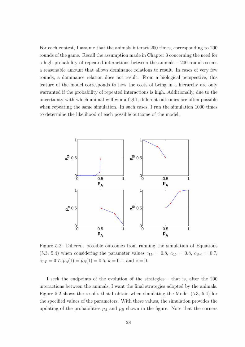
For each contest, I assume that the animals interact 200 times, corresponding to 200

rounds of the game. Recall the assumption made in Chapter 3 concerning the need for

a high probability of repeated interactions between the animals – 200 rounds seems

a reasonable amount that allows dominance relations to result. In cases of very few

rounds, a dominance relation does not result. From a biological perspective, this

feature of the model corresponds to how the costs of being in a hierarchy are only

warranted if the probability of repeated interactions is high. Additionally, due to the

uncertainty with which animal will win a fight, different outcomes are often possible

when repeating the same simulation. In such cases, I run the simulation 1000 times

to determine the likelihood of each possible outcome of the model.

0 0.5 10

0.5

1

pA

pB

0 0.5 10

0.5

1

pA

pB

0 0.5 10

0.5

1

pA

pB

0 0.5 10

0.5

1

pA

pB

Figure 5.2: Different possible outcomes from running the simulation of Equations

(5.3, 5.4) when considering the parameter values c1L = 0.8, c0L = 0.8, c1W = 0.7,

c0W = 0.7, pA(1) = pB(1) = 0.5, k = 0.1, and z = 0.

I seek the endpoints of the evolution of the strategies – that is, after the 200

interactions between the animals, I want the final strategies adopted by the animals.

Figure 5.2 shows the results that I obtain when simulating the Model (5.3, 5.4) for

the specified values of the parameters. With these values, the simulation provides the

updating of the probabilities pA and pB shown in the figure. Note that the corners

28

of each graph correspond to the different end-points of the N rounds of the game:

the corners (0,0), (1,0), (0,1) and (1,1) correspond to Dove–Dove, Hawk–Dove, Dove–

Hawk, and Hawk–Hawk, respectively.

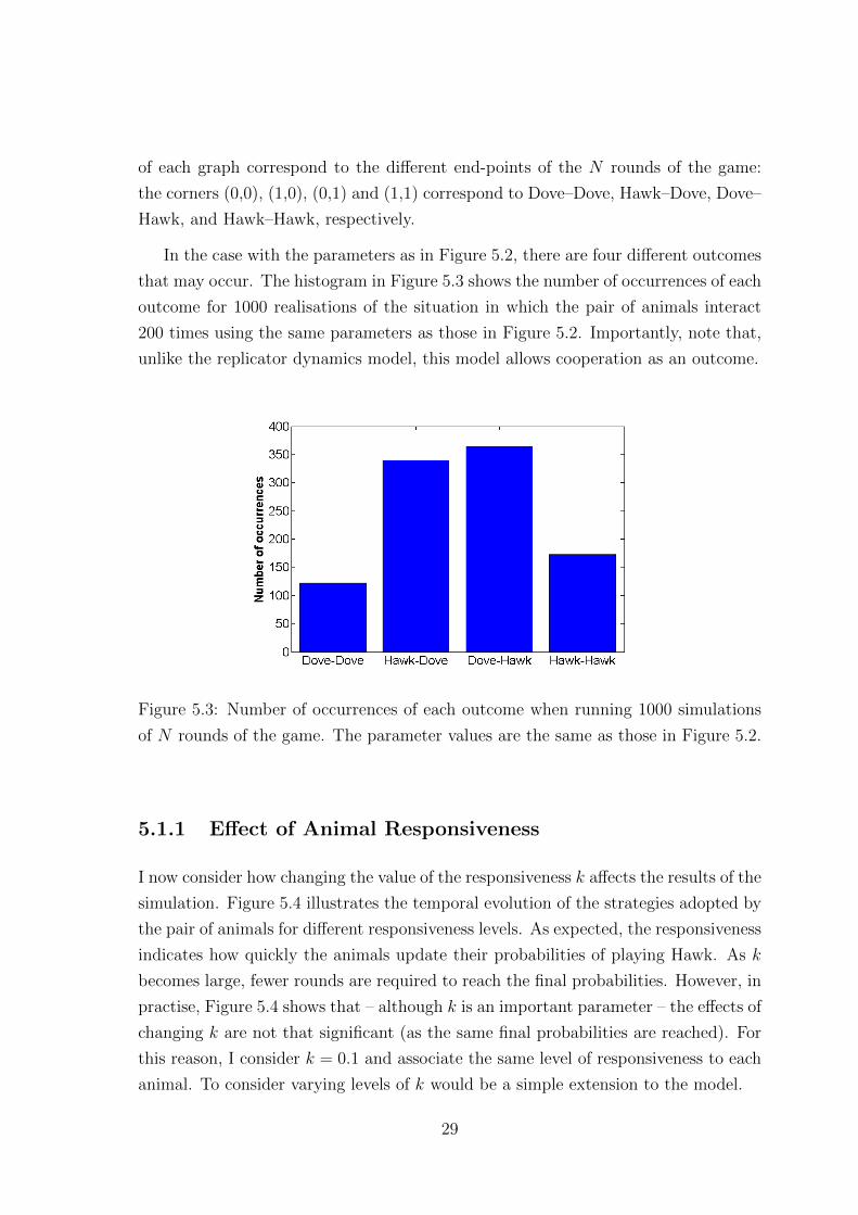
In the case with the parameters as in Figure 5.2, there are four different outcomes

that may occur. The histogram in Figure 5.3 shows the number of occurrences of each

outcome for 1000 realisations of the situation in which the pair of animals interact

200 times using the same parameters as those in Figure 5.2. Importantly, note that,

unlike the replicator dynamics model, this model allows cooperation as an outcome.

Figure 5.3: Number of occurrences of each outcome when running 1000 simulations

of N rounds of the game. The parameter values are the same as those in Figure 5.2.

5.1.1 Effect of Animal Responsiveness

I now consider how changing the value of the responsiveness k affects the results of the

simulation. Figure 5.4 illustrates the temporal evolution of the strategies adopted by

the pair of animals for different responsiveness levels. As expected, the responsiveness

indicates how quickly the animals update their probabilities of playing Hawk. As k

becomes large, fewer rounds are required to reach the final probabilities. However, in

practise, Figure 5.4 shows that – although k is an important parameter – the effects of

changing k are not that significant (as the same final probabilities are reached). For

this reason, I consider k = 0.1 and associate the same level of responsiveness to each

animal. To consider varying levels of k would be a simple extension to the model.

29

0 5 10 15 200

0.2

0.4

0.6

0.8

1

Time (interaction number)

Pro

ba

bili

ty o

f p

layi

ng

Ha

wk

Animal AAnimal B

0 5 10 15 200

0.2

0.4

0.6

0.8

1

Time (interaction number)

Pro

ba

bili

ty o

f p

layi

ng

Ha

wk

Animal AAnimal B

0 5 10 15 200

0.2

0.4

0.6

0.8

1

Time (interaction number)

Pro

ba

bili

ty o

f p

layi

ng

Ha

wk

Animal AAnimal B

0 5 10 15 200

0.2

0.4

0.6

0.8

1

Time (interaction number)

Pro

ba

bili

ty o

f p

layi

ng

Ha

wk

Animal AAnimal B

k=0.01

k=0.001

k=0.1

k=0.0001

Figure 5.4: Effects of varying responsiveness k for the parameters c1L = 0.3, c0L = 0.3,

c1W = 0.2, c0W = 0.2, pA(1) = pB(1) = 0.5, and z = 0.5.

5.2 Dominance of a Smaller Animal

In situations, when the smaller of the two animals wins an escalated contest early in

the N interactions, there are occasions where this results in an unexpected dominance

relation in which the smaller animal dominates. Importantly, this is not a flaw in the

model, as such occurrences are seen in nature (though they are rare) [41, 72].

The graph shown in the left panel of Figure 5.5 displays what would be expected

in a pair of animals with the size difference z = 0.5. That is, the larger animal A,

dominates animal B. The graph shown in the right panel of Figure 5.5 shows another

outcome that occurs but one that would not necessarily be expected: in this case,

animal B dominates animal A.

30

0 0.5 10

0.2

0.4

0.6

0.8

1

pA

p B

0 0.5 10

0.2

0.4

0.6

0.8

1

pA

p B

Figure 5.5: The left panel shows the expected dominance relation – the larger animal

dominates the smaller animal. The right panel shows that the smaller animal can

sometimes get lucky and win early on in the N rounds causing it to be the dominant

animal in the pair. The parameters used for these simulations are c1L = 0.3, c0L = 0.3,

c1W = 0.2, c0W = 0.2, pA(1) = pB(1) = 0.5, and z = 0.5.

5.3 Limitations of the Model

Recall the discussion in Chapter 1 concerning the levels of aggression that animals

show when initially grouped together. For this reason, I consider the case where

pA(1) = pB(1) = 1. In this situation, the simulations suggest that the only result

possible is continuous fighting – neither cooperation nor dominance relations occur.

HHHHH

HHHA

BDove Hawk

Dove (0.5,0.5) (0,1)

Hawk (1,0) (−0.25,−0.25)

Table 5.1: The expected game when considering parameter values c1L = 0.8, c0L =

0.8, c1W = 0.7, c0W = 0.7, pA(1) = pB(1) = 0.5, and z = 0. Importantly, note that

the expected payoffs in the Hawk–Hawk box are negative – this could correspond to

situations in which the costs of fighting are high, such as in lethal combat in animals

which might occur when the resource has a significant value [42].

This raises questions with the model, as in the case of the parameter values under

31

consideration, persistent fighting will just decrease the Darwinian fitness of both

animals. The game being played is shown in Table 5.1 and note that both entries in

the Hawk–Hawk box are negative. Thus, for both of the animals, it would be better

to simply withdraw from the contest by playing Dove instead. Although, this may

allow the animal’s opponent to win the entire resource, by playing the less aggressive

strategy, the animal will be able to ensure its Darwinian fitness does not decrease.

Thus, my model needs to incorporate the fact that an animal would not persistently

play a strategy that gives negative expected payoffs.

In the model that I have proposed, the reason why an animal stays at pA = 1 is

because the expected payoff is approximately equal to the payoff from the last round.

This is what prevents the player from switching to a better strategy. Thus, I need to

improve the model by modifying the way in which the behaviours are updated.

5.4 Modification of the Model

To summarise, good features of this model include that cooperation and dominance

relations are both possible outcomes. It also displays other realistic features such

as the way that smaller animals can sometimes become the dominant animal in a

pair, as well as that the outcomes of most pairwise contests are reached quite quickly.

However, there are also problems with this model. In cases where I am considering

parameter values that give a negative expected payoff from playing the game, the

model does not account for the fact that an animal would not stay at an outcome

that will always decrease its Darwinian fitness.

I gave an example where both animals were sticking to the strategy Hawk, even

though both were receiving negative expected returns. In such situations, it is more

realistic that an animal will just cooperate/withdraw from a fight. That way, although

the animal can only receive either half of the resource or even none of it, at least the

animal’s Darwinian fitness will not decrease. This motivates me to consider the cases

of positive and negative expected game returns separately.

I amend the model so that, for animal i, if

EGi (p

(n)A , p

(n)B ) < 0,

then animal i will play Dove (that is, pi(n+1) = 0) because it will always be better to

play Dove and get zero payoff then play Hawk and get a negative payoff. Figure 5.6

32

shows the simulation results obtained by using the amended model. When considering

the same parameters values as those used to create Figure 5.3, Figure 5.6 shows that

persistent fighting no longer occurs.

Figure 5.6: Number of occurrences of each outcome when running 1000 simulations

of the N rounds of the game with the modified model.

In the next model, I move away from the idea that an animal updates its behaviour

according to the difference between the payoff size received in the previous round and

the expected payoff. I need to account for situations in which there are negative

expected payoffs, as I showed in this chapter that there were cases in which the

animal would continue behaving in a way that was harmful for itself as long as the

payoffs were the expected ones. However, by considering the cases of positive and

negative expected game payoffs separately, more realistic outcomes were achieved.

Additionally, recall that the previous model assumed that the size of the asymme-

try z, was known to the animals. It is unrealistic to assume that all animals know the

size difference between themselves and their opponents. Instead, I will incorporate

uncertainty into my model and study a situation in which each animal estimates the

value of the asymmetry. It makes sense to incorporate uncertainty into the model

when trying to achieve cooperation as an outcome – surely, if animals are certain of

the size differences, then the biggest animal will be less likely to cooperate. By adding

uncertainty into the model, I might be able to achieve cooperation. This motivates

my next model (see Chapter 6), in which each animal’s behaviour is determined by

using its estimate for the asymmetry.

33

Chapter 6

Incorporating Uncertainty

I now consider the more realistic situation involving incomplete information, in which:

• the animals do not know each other’s probabilities of playing Hawk, and

• the animals do not know the true size of the asymmetry.

By using the downfall of the previous model as motivation, I consider how the

strategies adopted by animals evolve when faced with negative expected payoffs. I

showed in the static analysis that the ESSs depended on the sign of the expected

payoffs from fighting. In the context of animal behaviour, the negative payoffs could

correspond to situations in which the costs of fighting are high, such as in lethal

combat in animals which might occur when the resource has a significant value [42].

As the value of the resource increases, the relative costs of fighting decrease, as

the animals are prepared to fight more for the resource. Hence, what should be seen

in my model is that as the costs of fighting decrease, there should be an increased

likelihood that the behaviour of each animal evolves to Hawk. Alternatively, as the

costs of fighting increases (which might also be interpreted in my model as a decrease

in the value that the animals attach to the resource), the frequencies of fighting should

decrease.

In the case of negative expected payoffs from fighting, I need to determine the

optimal strategy for an animal to play. I have discussed that it is more beneficial for

an animal’s fitness that it play Dove in such a scenario rather than playing Hawk.

However, what is stopping an animal from waiting for its opponent to switch to the

cooperative strategy before obtaining the whole resource for itself by playing Hawk?

This is a similar problem to the iterated prisoner’s dilemma game that I consid-

ered in Chapter 2. Cooperation could be reached when each prisoner was scared of

defecting in case it triggered the other prisoner to defect as well. In the evolutionary

game that I am considering, if an animal plays the more aggressive strategy of Hawk

34

in the current round of the game, it must be careful of risking retaliation in later

rounds. Thus, by each animal being scared of receiving negative payoffs in the future,

they would rather play Dove than risk playing Hawk.

With this in mind, I now modify how the probability that each animal has of

playing Hawk updates after a round of the game. I need to determine the optimal

strategies to be played when the expected payoffs from fighting are positive, negative,

or zero.

From the static analysis, I have already seen that in cases where the expected

payoffs from fighting are positive, then the Hawk strategy is the best response to any

choice of strategy that its opponent might play. When the expected fighting payoffs

are zero, I again set the best strategy choice as Hawk. This is because if Dove is

played, then the animal can either receive a payoff of 0 or 0.5, whereas if Hawk is

played, it can receive a payoff of 0 or 1. Finally, when the entry is negative, I use the

earlier motivation as the reason why the Dove strategy is played.

Again, I use increment steps in order to change the strategy towards what the

animals thinks the optimal strategy is at each stage. Recall that δi denotes player i’s

expected payoff for fighting. Now, I find the probability that animal i plays Hawk by

using

p(n+1)i = p

(n)i + k ×

{0− p(n)i , if δi < 0,

1− p(n)i , if δi ≥ 0,(6.1)

for i = A,B. Thus, in situations in which the expected payoff for fighting is positive,

the probability for the next round will increase, whilst in situations where the expected

payoff for fighting is negative, the probability will decrease. I now incorporate the

idea that animals will not know the size of the asymmetry between themselves and

their opponent.

6.1 Updating the Asymmetry Estimates

I consider a scenario in which the true difference in body-size between the players

is not known initially. Each player starts by playing Hawk, and then by using the

results of the game, they update their perceptions of the real size difference. By using

such updated beliefs, I will be able to model how the behaviours of the animals evolve

over the rounds of the game. Recall that the size of asymmetry is important because

35

it has a significant effect on the expected payoffs from fighting. The probability that

each animal has of winning a fight depends on this value, which in turn affects the

estimated expected payoff from fighting and hence also the strategy to be played.

The asymmetry estimates are updated as follows:

z(n+1)i = z

(n)i + kz ×

1− z(n)i , if A wins a fight,

−1− z(n)i , if A loses a fight,

0, if no fight occurs,

(6.2)

where z(n)i is player i’s estimated value of the asymmetry z to be used in deciding the

strategy choice for round n. The parameter kz denotes the level of responsiveness of

an animal to updating the estimates of z (recall that the parameter k, which is seen

in Equation (6.1), denotes the level of responsiveness of an animal to updating the

probability of playing Hawk). The updating rate kz is the same for each animal.

6.2 Simulations

I assume that each animal initially estimates that the size difference between the

pair to be 0. Furthermore, changing this simplifying assumption would be an easy

modification to make in the proposed model. Each player starts with the same initial

estimate and then updates its estimates at the same rate and by using the same

information. This implies that when simulating the game, I should expect the animals

to have identical estimates in each round.

I run simulations of the new model for the situation in which the animals have

N = 200 interactions corresponding to N rounds of the game. Figure 6.1 shows the

results that I obtain by using the parameters values c0W = 0.1, c0L = 0.9, c1W = 0.1,

c1L = 0.4, z = 0.1, k = 0.1, and kz = 0.1.

The graph on the left of Figure 6.1 shows the evolution of the probabilities pA

and pB, whereas the graph on the right of the figure displays the updating of the

asymmetry estimates. I see that after N interactions, A plays the strategy Hawk,

whereas B plays the strategy Dove (i.e., there is a dominance relation).

36

0 50 100 150 2000

0.2

0.4

0.6

0.8

1

Time (interaction number)

Pro

ba

bil

ity

of

pla

yin

g H

aw

k

0 50 100 150 200−1

−0.5

0

0.5

1

Time (interaction number)E

sti

ma

te f

or

the

siz

e d

iffe

ren

ce

z

Animal AAnimal B

Animal AAnimal B

Figure 6.1: The left panel shows the changes in probabilities pA and pB over the N

rounds of the game. The right panel shows the updating of the estimates for the

asymmetry.

0 50 100 150 2000

0.2

0.4

0.6

0.8

1

Time (interaction number)

Pro

bab

ilit

y o

f p

layin

g H

aw

k

0 50 100 150 200−1

−0.5

0

0.5

1

Time (interaction number)

Esti

mate

fo

r th

e s

ize d

iffe

ren

ce z

Animal AAnimal B

Animal AAnimal B

Figure 6.2: Demonstration that the smaller animal can sometimes get lucky and win

early on in the N rounds causing it to be the dominant animal in the pair.

37

As with the previous model, Figure 6.2 (which uses the same parameter values as

in Figure 6.1) shows that this model also exhibits the realistic feature that there are

occasions where the smaller animal in a pair dominates. This happens if the smaller

animal wins early in the rounds, which causes its opponent (and itself) to believe that

the smaller animal is bigger than its true size.

0 50 100 150 2000

0.2

0.4

0.6

0.8

1

Time (interaction number)

Pro

ba

bil

ity

of

pla

yin

g H

aw

k

0 50 100 150 200−1

−0.5

0

0.5

1

Time (interaction number)

Es

tim

ate

fo

r th

e s

ize

dif

fere

nc

e z

Animal AAnimal B

Animal AAnimal B

Figure 6.3: Demonstration that the model can produce cooperation as a result.

Cooperation between animals should be expected when the costs of fighting are

high and the size difference between the animals is thought to be small (so that it

would be better to avoid a fight rather than risk injury). Figure 6.3 shows that this

model allows cooperation as an outcome. The parameters used for this simulation are

c0W = 0.6, c0L = 1, c1W = 0.5, c1L = 0.6, z = 0.2, k = 0.1, and kz = 0.1. The bump

in the probability of animal A playing Hawk (seen in the left panel of Figure 6.3)

occurs because A wins the first few fights. However, the updated value of estimated

z still gives a negative expected payoff, so the probability decreases towards zero –

cooperation.

One should note that in some of the results, the final estimate of z does not

correspond to the imposed size difference between the players. A good example of

this is given in Figure 6.2, where the final estimate is z = −0.1, whereas the true

asymmetry value is z = 0.1. One might expect that such an estimate would be closer

to the imposed size difference when there is more information available on which the

players can base their beliefs – that is, when more fights occur. Figure 6.4 shows the

38

results obtained when considering parameter values that give low costs of fighting

(and hence persistent aggressive behaviour).

0 50 100 150 2000

0.2

0.4

0.6

0.8

1

Time (interaction number)

Pro

bab

ility

of

pla

yin

g H

awk

0 50 100 150 200−1

−0.5

0

0.5

1

Time (interaction number)

Est

imat

e fo

r th

e si

ze d

iffe

ren

ce z

Animal AAnimal B

Animal AAnimal B

Figure 6.4: When the parameters chosen correspond to low fighting costs, differences

between the asymmetry estimates and the true value of the asymmetry can still occur.

The parameter values used in this simulation are c0W = 0.05, c0L = 0.1, c1W = 0.05,

c1L = 0.1, z = 0.3, k = 0.1, and kz = 0.1.

Additionally, Figure 6.4 further motivates me to consider another updating rule

for the estimates of the asymmetry. It is important to have a good updating rule

for the estimates of the asymmetry, as the estimated size difference between a pair

of animals plays a big role in my modelling of strategy choices. Thus, I now seek to

improve this part of the model. To update more accurately, I will now incorporate

Bayesian updating into the model.

6.3 Bayesian Updating

Recall that z is the size difference defined as

z = size of animal A− size of animal B.

I revisit a situation in which animals A and B each estimate the size difference z

and update their estimates after each round of the game. In the previous model, I

39

updated z simply by increasing it slightly in cases in which animal A wins a fight

and decreasing it slightly when A loses a fight. Another method that can be used to

update the size difference estimates from the outcomes of the game is called ‘Bayesian

updating’ in which beliefs about the true value of the size difference z can be expressed

as a probability and are updated if new information becomes available [31].

Bayesian updating entails using conditioning to update prior beliefs by using any

new information obtained about the uncertain hypothesis. The animals express their

beliefs about the size of z in terms of a probability P (Hypothesis). New evidence

then yields a new estimate: P (Hypothesis|Evidence).

Bayesian updating uses Bayes’ rule, which is

P (Hypothesis|Evidence) =P (Hypothesis ∩ Evidence)

P (Evidence)

=P (Evidence|Hypothesis) × P (Hypothesis)

P (Evidence).

The P (Hypothesis|Evidence) term is called the ‘posterior’ and the P (Hypothesis)

term is called the ‘prior’. Bayesian updating involves iterating the rule above by

updating the prior belief with the posterior belief. For each value of z, I calculate

P (z|fight outcome) =P (z ∩ fight outcome)

P (fight outcome)

=P (fight outcome|z) × P (z)

P (fight outcome), (6.3)

which gives a probability distribution for z. By finding the peak of the posterior, I

can determine the most likely value of z, and I will use this as the updated estimate

of z. In the simulations, I take the prior probability distributions to be Gaussian

distributions centred at the initial estimates of z.

Figure 6.5 shows the results obtained by simulating a situation with low costs of

fighting (which yields more fighting and thus more information with which to update

asymmetry estimates). Pseudo-code for simulating the model consisting of Equation

(6.1) and Bayesian updating is given in the Appendix. Figure 6.5 shows the evolution

of the probability distribution for the value of z as the number of interactions between

a pair of animals increases. As N increases, since more fights occur, the peak of the

posterior also grows, as the animals gradually become more confident about their

beliefs of the true value of z. This is the case because each fight provides additional

information with which to update estimates. As before, the peak may not narrow

40

(i.e. animals may not reach certainty) if costs are high and they stop fighting after a

smaller number of rounds.

Figure 6.5: Bayesian update of z over the N rounds. The parameter values are

c0W = 0.02, c0L = 0.05, c1W = 0.02, c1L = 0.03, z = 0.5, and k = 0.1.

To summarise, by adding uncertainty into the problem, I have developed a model

that allows both dominance relations and cooperation as outcomes of pairwise con-

tests. In this chapter, I used Bayesian updating to help model how an animal’s

behaviour can change between the different rounds of a game. A possible criticism of

this method is that it is unreasonable to assume that animals will update their beliefs

according to Bayes’ rule. However, research has shown that animals are ‘capable’ of

Bayesian updating [69].

All that is left to do is to model how a dominance hierarchy of an animal group

can be formed using such interactions. I discuss this topic in Chapter 7.

41

Chapter 7

Hierarchy Formation

I now construct a dominance hierarchy in an animal group by examining the outcomes

of a round-robin style tournament, in which each animal plays the game with every

other animal. One can interpret this as a game on a complete network, in which

each animal is a node and each edge indicates a game between the associated set of

animals. If I consider a group consisting of M animals, this implies that there are12M(M − 1) pairwise interactions. I also assume that such encounters are repeated

N times, so there are 12M(M − 1) plays of the game during each of N rounds.

Although there is limited amount of resource available, I assume that there is still

enough to satisfy the amount required for a set up of a dominance hierarchy, whilst

also being sufficiently large so that the costs of fighting in the game remain fixed.

7.1 Calculating the Hierarchy Order

I discussed in Chapter 4 how a dominance hierarchy could be constructed using

all dominance relations or cooperative relations between all pairs from the group.

However, as the following example illustrates, there is difficulty in ordering animals

into a hierarchy if the dominance relations are not transitive.

7.1.1 Example

Consider a group of 4 animals and suppose that the resulting strategy pairs given by

the model are those shown in Table 7.1. Summarising these results in the form of a

picture (where an arrow A → B indicates that B dominates A and a line with no

direction indicates that there is no dominance relation), Figure 7.1 shows that not

all of the dominance relations are transitive. For instance, 1 dominates 2 and 1 is

indifferent in ranking to 4, but 2 dominates 4.

42

1 2 3 4

1 - H-D D-H D-D

2 - - D-H H-D

3 - - - H-D

4 - - - -

Table 7.1: The strategy pairs resulting from N rounds of the game, where ‘D’ repre-

sents a Dove strategy and ‘H’ represents a Hawk strategy.

Figure 7.1: Illustration of the dominance relations given in Table 7.1.

Recall the notation introduced in Chapter 5 – p(n)i denotes the strategy played by

animal i in the nth round. A basic way to form the dominance hierarchy, even when

the relations are not transitive, is by assigning the value p(N)A − p(N)

B to the strategy

pair end-points obtained from the simulations. This provides me with a measure that

I can use when modelling the rankings of the animals. Table 7.2 shows the values

that I assign to each strategy pair.

Strategy pair Assigned Value

Dove–Dove 0

Dove–Hawk −1

Hawk–Dove 1

Hawk–Hawk 0

Table 7.2: The values that I assign to each possible final strategy pair.

43

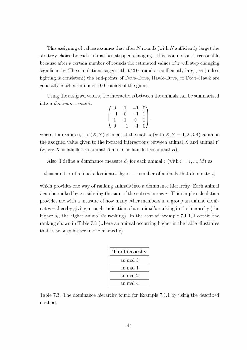
This assigning of values assumes that afterN rounds (withN sufficiently large) the

strategy choice by each animal has stopped changing. This assumption is reasonable

because after a certain number of rounds the estimated values of z will stop changing

significantly. The simulations suggest that 200 rounds is sufficiently large, as (unless

fighting is consistent) the end-points of Dove–Dove, Hawk–Dove, or Dove–Hawk are

generally reached in under 100 rounds of the game.

Using the assigned values, the interactions between the animals can be summarised

into a dominance matrix 0 1 −1 0−1 0 −1 11 1 0 10 −1 −1 0

,

where, for example, the (X, Y ) element of the matrix (with X, Y = 1, 2, 3, 4) contains

the assigned value given to the iterated interactions between animal X and animal Y

(where X is labelled as animal A and Y is labelled as animal B).

Also, I define a dominance measure di for each animal i (with i = 1, ...,M) as

di = number of animals dominated by i − number of animals that dominate i,

which provides one way of ranking animals into a dominance hierarchy. Each animal

i can be ranked by considering the sum of the entries in row i. This simple calculation

provides me with a measure of how many other members in a group an animal domi-

nates – thereby giving a rough indication of an animal’s ranking in the hierarchy (the

higher di, the higher animal i’s ranking). In the case of Example 7.1.1, I obtain the

ranking shown in Table 7.3 (where an animal occurring higher in the table illustrates

that it belongs higher in the hierarchy).

The hierarchy

animal 3

animal 1

animal 2

animal 4

Table 7.3: The dominance hierarchy found for Example 7.1.1 by using the described

method.

44

The dominance measure that I have used is called the Netto score in [39] and it

is important to note that this method of ranking the animals will not always lead to

an unambiguous hierarchy, such as the one shown in Table 7.3. How should a model

account for cases in which there is a draw in the dominance measure between two or

more animals?

One way in which these draws can be eliminated from the hierarchy is by calcu-

lating the power, as explained in [46]. One should note that since such calculations

depend on taking powers of a dominance matrix, the matrix needs to be constructed

in a slightly different way from before in order for the power to be meaningful (more

details can be found in [46]).

However, from a biological perspective, a draw in the dominance measure may

correspond to cases where there are no stable dominance relations between the draw-

ing animals. Thus, in such a situation one animal does not rank higher or lower than

another animal as they might keep fighting. One example of how this might occur,

is when the size of the asymmetry between the animals is small.

To summarise, I have used the Hawk–Dove model as a tool with which to build

a dominance hierarchy. In this section, I have discussed one way of modelling a

dominance hierarchy. It is important to note that different dominance hierarchies

can be achieved using different ranking methods.

Similar to issues in other fields, such as determining how to design voting systems

[11] or how to rank sports teams [14], there is debate over which type of dominance

ranking procedure is best. In the context of animal dominance, some comparative

study has already been conducted in order to investigate the relative performance of

various different ranking methods (see, for example, [5]).

Earlier, I discussed the Netto score, but there are superior measures to use in

the modelling of a dominance hierarchy with the use of dominance matrices [39] or

without the use of dominance matrices [49]. One example (which also uses dominance

matrices) is the David’s score in [39], which is an extension of the method that I have

discussed in this chapter. However, these more advanced methods are beyond the

scope of this thesis and more information can be found in [5] and [39].

45

Chapter 8

Discussion

I have shown that my model allows both cooperation and dominance relations as out-

comes and have considered the modelling of the formation of a dominance hierarchy.

In this chapter, I investigate how much asymmetry is required to make qualitative

differences in the relative frequencies of cooperation versus dominance hierarchies.

My model depends on the expected payoff from fighting, which itself depends

on the value of the asymmetry. Thus, one would expect that the asymmetry plays

a significant role in determining which model outcomes are possible. Figures 8.1–

8.2 display the effect that changing the parameters has on the possible outcomes of

the model, where I have used the same colours as in Chapter 4. The orange region

corresponds to the parameter values that give the Hawk–Hawk end-point, the light

blue region corresponds to the parameter values that give the Hawk–Dove endpoint,

and the yellow region corresponds to the parameter values that give the Dove–Hawk

end-point. The dark blue region in the figures corresponds to the parameter values

that give Dove–Dove (cooperation) as a result.

In Figures 8.1 and 8.2, note that for each value of the cost parameter considered,

there is a window of values for the asymmetry in which cooperation can occur. This

window increases as the cost parameter on the vertical axis increases. From a bi-

ological perspective, this corresponds to the fact that an animal is more willing to

cooperate when the injury risks are higher. Additionally, it can be seen from com-

paring the two panels in each figure that increasing the fixed cost parameters also (as

expected) increases the relative frequency of cooperation versus dominance relations.

My model gives the desired results and has features that correspond to what would

be expected biologically. Naturally, now that a reasonable model has been developed,

one would want to test it using real data, though an important issue arises (see the

discussion below). The parameters in my final model are:

• the asymmetry z;

46

• the responsiveness of the animal k; and

• the cost parameters c0L, c1L, c0W , and c1W .

To test my model, I require reasonable values for the above parameters to use in the

simulation of a dominance hierarchy. Research suggests that body-size distributions

tend to be right-skewed log-normal distributions [17, 45]. Thus, for the simulations,

one could draw the body-sizes of each animal from such a distribution and then

calculate the size of the asymmetry between each pair of animals.

Also, research into the responsiveness of animals to environmental stimuli has

been carried out with many different species [74]. However, something that prevents

me from having a testable hypothesis is a lack of data concerning the values of the

cost parameters. How could such parameters be meaningfully measured?

This is a limitation of the model, but it should be noted that this is also a limita-

tion of this entire field. Due to the difficulty in measuring factors such as the costs of

fighting, models depending on these parameters cannot be tested easily against obser-

vational research. However, this problem can be reduced by considering ‘surrogate’

cost parameters.

Since longer fights imply that it ‘costs’ more for an animal to be involved, one

commonly used surrogate parameter is the ‘duration of an escalated contest’ [34].

Other examples include calculations involving the heartbeat rate of the animals in-

volved [59]. Thus, a natural extension to my model would be to use such surrogate

parameters to facilitate testing its predictions against observations.

Despite such limitations, there are also good features of the proposed model. In

particular, it provides a sound foundation that can easily be built upon. For example,

one might want to make a modification to incorporate more realistic characteristics

such as changing animal sizes.

Furthermore, the model that I have developed is ‘unified’ in the sense that was

discussed in Chapter 2. Not only does it model the formation of a dominance hier-

archy, but it also easily incorporates other features such as the introduction of a new

animal to the group. In such a scenario, there is usually a high level of ‘in-group’

aggression shown to the new individual [19, 57]. This is represented in my hierarchy

model by the way that the individual will have to compete with every member in

order for the individuals to obtain information about their relative fighting abilities.

47

Figure 8.1: Effects that the asymmetry has on the relative frequency of cooperation

versus dominance hierarchies, whilst varying the cost parameter c1L. The parameter

values used for the left panel are c0L = 0.2, c0W = 0.1, and c1W = 0.1. The parameter

values used for the right panel are c0L = 0.9, c0W = 0.7, and c1W = 0.6. The orange,

light blue, yellow, and dark blue regions correspond to the parameter values that give

Hawk–Hawk, Hawk–Dove, Dove–Hawk, and Dove–Dove end-points, respectively.

Figure 8.2: Effects that the asymmetry has on the relative frequency of cooperation

versus dominance hierarchies, whilst varying the cost parameter c0W . The parameter

values used for the left panel are c0L = 0.1, c1W = 0.1, and c1L = 0.2. The parameter

values used for the right panel are c0L = 0.3, c1W = 0.3, and c1L = 0.5. The regions

are coloured as those in Figure 8.1.

48

Chapter 9

Conclusion

The aim of this thesis was to develop a simple model for the occurrence of cooperation

and dominance hierarchies in animal groups, whilst accounting for possible individual

asymmetries between members. To do so, I first investigated the standard approaches

that already existed in this field. By conducting a static analysis, which involved the

concept of an evolutionary stable strategy, and a dynamic analysis, which involved

the replicator dynamics model, I showed that such models did not allow cooperation

to occur. This motivated me to develop a new model.

My final model incorporates the fact that it is unlikely for animals to persistently

risk injury in situations in which fighting would give a negative expected payoff. I

also incorporated the feature that animals are unlikely to know the true value of size

asymmetries. By playing the game and by being involved in fights, animals gain

more information with which they can update their asymmetry estimates. The final

proposed model allowed cooperation and dominance relations to result from pairwise

interactions between animals. Using the results of these interactions, I then discussed

how a dominance hierarchy could be formed.

The biggest limitation of the model is a lack of real data available concerning

the values of the cost parameters that feature in the game, but this is a weakness

of the field and not the model. The evolution of the behaviour that animals display

will depend on the relative size of costs and benefits that are associated to adopting

the different behaviours. Therefore, the cost parameters are justified and cannot be

removed from the model because they have a critical role in the modelling of the

animals’ behaviour. As discussed in Chapter 8, ‘surrogate’ cost parameters can be

used to provide a testable hypothesis. This is an advantage with a game-theoretic

model – they easily provide explicit predictions to be tested [66].

There are also many other possible extensions to this thesis. For instance, I only

considered one type of asymmetry between animals. Another interesting asymmetry

to consider would be to incorporate the feature that animals need not necessarily

49

value a resource in the same way. Further extensions could include relaxing some

of the assumptions made in the model. For example, it would be interesting to

relax the pairwise contests assumption and consider bystander effects – an animal

that observes other animals’ contests will have more information. This has been

considered in some hierarchy models, such as [25], but it would be interesting to

see the effects that bystanders have on the relative frequencies of cooperation versus

dominance hierarchies. Additionally, the modelling of the formation of a dominance

hierarchy could be extended by considering other forms of tournaments beyond a

round-robin style tournament.

To conclude, I have studied how game theory can be applied to the problem of

cooperation versus dominance hierarchies in animals to provide a framework in which

different types of animal behaviour can be easily analysed. I developed a novel model

and explored how the asymmetry of body-size differences can play a significant role

in determining the outcomes of interactions between members of animal groups. I

also made an original connection between the modelling the formation of a dominance

hierarchy and the Hawk–Dove model. Most importantly, this model provides a solid

foundation upon which to build future work.

50

Appendix: Pseudo-code for

Simulating Model (6.1)

In this appendix, I give the pseudo-code for simulating the Model (6.1) using Bayesian

updating. Consider the situation in which there are N interactions between two

animals A and B. The cost parameters of fighting are c0L, c1L, c0W , and c1W . Also,

the responsiveness of the animals is k and the true size difference is z.

1. Calculate the probability that each animal has of winning a fight (pAwinsand

pBwins) by using (Equations (3.1) and (3.2))

pAwins=

1

2z +

1

2and pBwins

=1

2− 1

2z.

2. Set the initial estimates of the size difference,

z(1)A and z

(1)B

, for animal A and animal B, respectively.

3. Set the initial probabilities of playing Hawk,

pA(1) and pB(1)

, for animal A and animal B, respectively.

4. The animals play a round of the game. Determine the strategies that each

animal adopts by using pA(1) and pB(1). If a fight occurs (both animals play

Hawk), then determine the winner of the fight by using pAwinsand pBwins

. Record

the results of this round of the game, and in particular record the winner of a

fight if one occurs.

5. For i = 2, ..., N (the 2nd to N th interactions)

• Use the outcomes of the previous round of the game to calculate the next

estimates for the size difference – z(i)A and z

(i)B – by using Bayes’ rule (Equa-

tion (6.3)).

51

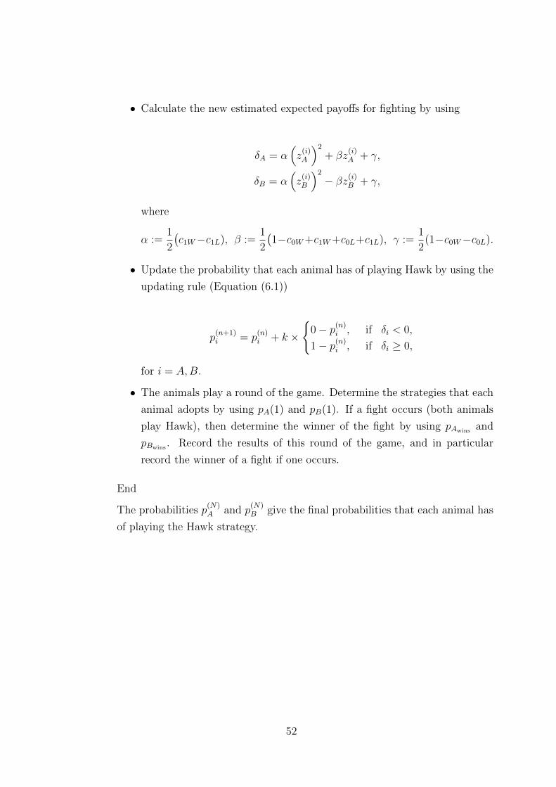
• Calculate the new estimated expected payoffs for fighting by using

δA = α(z(i)A

)2+ βz

(i)A + γ,

δB = α(z(i)B

)2− βz(i)B + γ,

where

α :=1

2

(c1W−c1L), β :=

1

2

(1−c0W +c1W +c0L+c1L), γ :=

1

2(1−c0W−c0L).

• Update the probability that each animal has of playing Hawk by using the

updating rule (Equation (6.1))

p(n+1)i = p

(n)i + k ×

{0− p(n)i , if δi < 0,

1− p(n)i , if δi ≥ 0,

for i = A,B.

• The animals play a round of the game. Determine the strategies that each

animal adopts by using pA(1) and pB(1). If a fight occurs (both animals

play Hawk), then determine the winner of the fight by using pAwinsand

pBwins. Record the results of this round of the game, and in particular

record the winner of a fight if one occurs.

End

The probabilities p(N)A and p

(N)B give the final probabilities that each animal has

of playing the Hawk strategy.

52

Bibliography

[1] Abbott, J.C., Dunbrack, R.L. and Orr, C.D. The Interaction of Size and Experience

in Dominance Relationships of Juvenile Steelhead Trout (Salmo gairdneri). Behaviour,

Vol. 92, pp. 241–253, 1985.

[2] Accinelli, E. and Sanchez Carrera, E.J. On evolutionarily stable strategies and replicator

dynamics in asymmetric two-population games. Department of Economics - dECON,

Working papers 1010, 2010.

[3] Adami, C. and Hintze, A. Winning isn’t everything: Evolutionary stability of Zero

Determinant strategies. arXiv:1208.2666v1, 2012.

[4] Axelrod, R. and Hamilton, W.D. The Evolution of Cooperation. Science, New Series,

Vol. 211(2289), pp. 1390–1396, 1981.

[5] Bang, A., Deshpande, S., Sumana, A. and Gadagkar, R. Choosing an appropriate index

to construct dominance hierarchies in animal societies: a comparison of three indices.

Animal Behaviour, Vol. 79, pp. 631–636, 2010.

[6] Benson-Amram, S., Heinen, V.K., Dryer, S.L. and Holekamp, K.E. Numerical assess-

ment and individual call discrimination by wild spotted hyenas (Crocuta crocuta). Ani-

mal Behaviour, Vol. 82, pp. 743–752, 2011.

[7] Blumstein, D.T. Group living. Encyclopedia of evolution, Oxford University Press, pp.

448–450, 2002.

[8] Bomze, I.M., Schuster, P. and Sigmund, K. The role of Mendelian genetics in strategic

models on animal behaviour. Journal of Theoretical Biology, Vol. 101(1), pp. 19–38,

1983.

[9] Braddock, J.C and Braddock, Z.I. Aggressive Behavior among Females of the Siamese

Fighting Fish, Betta splendens. Physiological Zoology, Vol. 28(2), pp. 152–172, 1955.

[10] Brams, S.J. Game Theory and Politics. Dover Publications, 2004.

[11] Brams, S.J. Mathematics and Democracy: Designing Better Voting and Fair-Division

Procedures. Princeton University Press, 2007.

[12] Broom, M. A unified model of dominance hierarchy formation and maintenance. Jour-

nal of Theoretical Biology, Vol. 219, pp. 63–72, 2002.

53

[13] Caldwell, R.L. and Dingle, J. The influence of size differential on agonistic encounters

in the mantis shrimp, Gonodactylus viridis. Behaviour, Vol. 69, pp. 255–264, 1979.

[14] Cassady, C.R., Maillart, L.M. and Salman, S. Ranking Sports Teams: A Customizable

Quadratic Assignment Approach. Interfaces, Vol. 35(6), pp. 497–510, 2005.

[15] Chapais, B. Alliances as a means of competition in primates: evolutionary, develop-

mental and cognitive aspects. Yearbook of Physical Anthropology, Vol. 38, pp. 115–136,

1995.

[16] Chase, I.D., Tovey, C., Spangler-Martin, D. and Manfredonia, M. Individual differences

versus social dynamics in the formation of animal dominance hierarchies. Proceedings

of the National Academy of Sciences USA, Vol. 99, pp. 5744–5749, 2002.

[17] Clauset, A. How large should whales be? arXiv:1207.1478v1, 2012.

[18] Clutton-Brock, T.H., Albon, S.D., Gibson, R.M. and Guinness, F.E. The logical stag:

Adaptive aspects of fighting in red deer (Cervus elaphus L.). Animal Behaviour, Vol. 27

(1), pp. 211–225, 1979.

[19] Cords, M. Friendship among Adult Female Blue Monkeys (Cercopithecus mitis). Be-

haviour, Vol. 139, pp. 291–314, 2002.

[20] Darwin, C. Natural Selection. Bibliolis Books, pp. 27–32, 2010.

[21] Dawkins, M.S. Do assymmetries destabilize the Prisoner’s Dilemma and make recip-

rocal altruism likely? Animal Behaviour, Vol. 80, pp. 339–341, 2010.

[22] Dobson, S. and Goddard, J. The Economics of Football. Cambridge University Press,

pp. 106–130, 2nd Edition, 2011.

[23] Drews, C. The concept and definition of dominance in animal behaviour. Behaviour,

Vol. 125, pp. 283–313, 1993.

[24] Dugatkin, L.A. The Evolution of Cooperation. BioScience, Vol. 47(6), pp. 355–362,

1997.

[25] Dugatkin, L.A. and Earley, R.L. Group fusion: the impact of winner, loser, and by-

stander effects on hierarchy formation in large groups. Behavioral Ecology, Vol. 14(3),

pp. 367–373, 2003.

[26] Eichberger, J. Game Theory for Economists. Academic Press, 1993.

[27] Foster, W.A. Duelling aphids: intraspecific fighting in Astegopteryx minuta (Ho-

moptera: Hormaphididae). Animal Behaviour, Vol. 51, pp. 645–655, 1996.

54

[28] Freeman, S. Biological Science. Prentice Hall, pp. 418–419, 1st Edition, 2002.

[29] Gadagkar, R. Dominance hierarchy and division of labour in the social wasp, Ropalidida

marginata (Lep.)(Hymenoptera: Vespidae). Current Science, Vol. 49(20), pp. 772–775,

1980.

[30] Godard, R. Tit for tat among neighboring hooded warblers. Behavioral Ecology and

Sociobiology, Vol. 33, pp. 45–50, 1993.

[31] Greenberg, E. Introduction to Bayesian Econometrics. Cambridge University Press,

pp. 24–25, 2007.

[32] Greenberg, N., Chen, T. and Crews, D. Social Status, gonadal state, and the adrenal

stress response in the lizard, Anolis carolinensis. Hormones and Behavior, Vol. 18, pp.

1–11, 1984.

[33] Guhl, A.M. The social order of chickens. Scientific American, Vol. 194(2), pp. 42–46,

1956.

[34] Hack, M.A. The energetic costs of fighting in the house cricket, Acheta domesticus L.

Behavioral Ecology, Vol. 8, pp. 28–36, 1997.

[35] Haigh, J. Taking Chances: Winning with Probability. Oxford University Press, pp.

116–123, 2003.

[36] Halpern, J.Y. Computer Science and Game Theory: A Brief Survey, A Palgrave Dic-

tionary of Economics, 2008.

[37] Hammerstein, P. and Selten, R. Chapter 28 in Handbook of Game Theory with Eco-

nomic Applications. Elsevier, Vol. 2, pp. 929–993, 1994.

[38] Hansen, A.J. Fighting Behavior in Bald Eagles: A Test of Game Theory. Ecology, Vol.

67, pp. 787–97, 1986.

[39] Hemelrijk, C.K., Wantia, J. and Gygax, L. The construction of dominance order:

comparing performance of five methods using an individual-based model. Behaviour, Vol.

142, pp. 1037–1058, 2005.

[40] Hofbauer, J. and Sigmund, K. Evolutionary Game Dynamics. Bulletin of the American

Mathematical Society, Vol. 40(4), pp. 479–519, 2003.

[41] Hughes, M. Size assessment via a visual signal in snapping shrimp. Behavioral Ecology

and Sociobiology, Vol. 38, pp. 51–57, 1996.

55

[42] Innocent, T.M., West, S.A., Sanderson, J.L., Hyrkkanen, N. and Reece, S.E. Lethal

combat over limited resources: testing the importance of competitors and kin. Behavioral

Ecology, Vol. 22(5), pp. 923–931, 2011.

[43] Ioannou, C.C., Guttal, V. and Couzin, I.D. Predatory Fish Select for Coordinated

Collective Motion in Virtual Prey. Science 1218919, 2012.

[44] Issa, F.A., Adamson, D.J. and Edwards, D.H. Dominance hierarchy formation in ju-

venile crayfish procambarus clarkii. Journal of Experimental Biology, Vol. 202(24), pp.

3497–3506, 1999.

[45] Kozlowski, J. and Gawelczyk, A.T. Why are species body size distributions usually

skewed to the right? Functional Ecology, Vol. 16, pp. 419–432, 2002.

[46] Litke, R.E. Dominance matrices for determining winners of debate tournaments. The

Speech Teacher, Vol. 15(4), pp. 295–298, 1966.

[47] Milinski, M. Tit for tat in sticklebacks and the evolution of cooperation. Nature, Vol.

325, pp. 433–435, 1987.

[48] Nelissen, M.H.J. Structure of the Dominance Hierarchy and Dominance Determining

”Group Factors” in Melanochromis auratus (Pisces, Cichlidae). Behaviour, Vol. 94, pp.

85–107, 1985.

[49] Neumann, C., Duboscq, J., Dubuc, C., Ginting, A., Irwan, A.M., Agil, M., Widdig,

A. and Engelhardt, A. Assessing dominance hierarchies: validation and advantages of

progressive evaluation with Elo-rating. Animal Behaviour, Vol. 82, pp. 911–921, 2011.

[50] Nijman, V. and Heuts, B.A. Effect of environmental enrichment upon resource holding

power in fish in prior residence situations. Behavioural Processes, Vol. 49, pp. 77–83,

2000.

[51] Nowak, M. An evolutionarily stable strategy may be inaccessible. Journal of Experi-

mental Biology, Vol. 142(2), pp. 237–241, 1990.

[52] Osborne, M.J. and Rubinstein, A. A Course in Game Theory. The MIT Press, pp.

48–52, 1999.

[53] Ottronen, M. The effect of body size on the outcome of fights in burying beetles

(Necrophorus). Annales Zoologici Fennici, Vol. 25, pp. 191–201, 1988.

[54] Pagel, M. and Dawkins, M.S. Peck orders and group size in laying hens: futures con-

tracts for non-aggression. Behavioural Processes, Vol. 40, pp. 13–25, 1997.

56

[55] Potegal, M. and Knutson, J.F. The Dynamics of Aggression: Biological and Social

Processes in Dyads and Groups. Lawrence Erlbaum Associates, pp. 73–111, 1994.

[56] Radespiel, U. and Zimmerman, E. Female dominance in captive gray mouse lemurs

(Microcebus murinus). American Journal of Primatology, Vol. 54(4), pp. 181–92, 2001.

[57] Rajecki, D.W, Ivins, B. and Rein, B. Social Discrimination and Aggressive Pecking in

Domestic Chicks. Journal of Comparative and Phonological Psychology, Vol. 90(5), pp.

442–452, 1960.

[58] Reebs, S.G. Aggression in Fishes. University de Moncton, Canada, 2008.

[59] Rovero, F., Hughes, R.N., Whiteley, N.M. and Chelazzi, G. Estimating the energetic

cost of fighting in shore crabs by noninvasive monitoring of heartbeat rate. Animal Be-

haviour, Vol. 59, pp. 705–713, 1999.

[60] Samuelson, L. Evolutionary Games and Equilibrium Selection. The MIT Press, pp.

1–81, 1998.

[61] Samuelson, L. and Zhang, J. Evolutionary Stability in Asymmetric Games. Journal of

Economic Theory, Vol. 57, pp. 363–391, 1992.

[62] Selten, R. A Note on Evolutionary Stable Strategies in Asymmetric Animal Conflicts.

Journal of Theoretical Biology, Vol. 84, pp. 93–101, 1980.

[63] Seyfarth R.M. and Cheney, D.L. Grooming, alliances and reciprocal altruism in vervet

monkeys. Nature, Vol. 308, pp. 541–543, 1984.

[64] Smith, J.M. Evolution and the Theory of Games. Cambridge University Press, pp.

1–54, 1982.

[65] Stamps, J.A. The Relationship between Resource Competition, Risk, and Aggression in

a Tropical Territorial Lizard. Ecology, Vol. 58(2), pp. 349–358, 1977.

[66] Stuart-Fox, D. Testing game theory models: fighting ability and decision rules in

chameleon contests. Proceedings of the Royal Society of London, Series B, Vol. 273,

pp. 1555–1561, 2006.

[67] Tarpy, D.R., Gilley, D.C. and Seeley, T.D. Levels of selection in a social insect: a

review of conflict and cooperation during honey bee (Apis mellifera) queen replacement.

Behavioral Ecology and Sociobiology, Vol. 55, pp. 513–523, 2004.

[68] Taylor, P.D. and Jonker, L.B. Evolutionarily stable strategies and game dynamics.

Mathematical Biosciences, Vol. 40, pp. 145–156, 1978.

57

[69] Valone, T.J. Are animals capable of Bayesian updating? An empirical review. Oikos,

Vol. 112, pp. 252–259, 2006.

[70] Vehrencamp, S.L. A model for the evolution of despotic versus egalitarian societies.

Animal Behaviour, Vol. 31, pp. 667–682, 1983.

[71] Weibull, J.W. Evolutionary Game Theory. The MIT Press, pp. 1–93, 1997.

[72] Wells, M.S. Effects of body size and resource value on fighting behaviour in a jumping

spider. Animal Behaviour, Vol. 36, pp. 321–326, 1988.

[73] Wilkinson, G.S. Reciprocal food sharing in the vampire bat. Nature, Vol. 308, pp. 181–

184, 1984.

[74] Wolf, M., van Doorn, G.S. and Weissing, F.J. Evolutionary emergence of responsive

and unresponsive personalities. Proceedings of the National Academy of Sciences USA,

Vol. 105(41), pp. 15825–15830, 2008.

[75] Yasukawa, K. and Bick, E.I. Dominance hierarchies in dark-eyed junkos (Junco hye-

malis): a test of a game-theory model. Animal Behaviour, Vol. 31, pp. 439–448, 1983.

58