cooperating tools for wireless sensor networks343921/fulltext01.pdfit 10 018 examensarbete 30 hp maj...
TRANSCRIPT

IT 10 018
Examensarbete 30 hpMaj 2010
Cooperating Tools for Wireless Sensor Networks
Qian Li
Institutionen för informationsteknologiDepartment of Information Technology


Teknisk- naturvetenskaplig fakultet UTH-enheten Besöksadress: Ångströmlaboratoriet Lägerhyddsvägen 1 Hus 4, Plan 0 Postadress: Box 536 751 21 Uppsala Telefon: 018 – 471 30 03 Telefax: 018 – 471 30 00 Hemsida: http://www.teknat.uu.se/student
Abstract
Cooperating Tools for Wireless Sensor Networks
Qian Li
Wireless Sensor Network (WSN) simulators, testbeds, and environment simulatorsare indispensable tools for WSN research. Existing WSN tools were developed withdifferent purposes without the intention of cooperation. Nevertheless, thedevelopment of a WSN technology (e.g, a middleware, a protocol, or an application)usually requires the cooperation among multiple tools. This calls upon a breaking ofthe incompatible barriers between any pair of tools.
In this thesis, I propose the Common Input and Output integration approach (theCIO approach). This approach attempts to define a standard configuration file formatcontaining input and output data common to WSN tools. In hope that by supportingthis standard configuration file format, tools can cooperate. The WiseML [23] formatdefined by the WISEBED [29] project is fully in compliance with the requirement ofthe CIO format. Therefore, it is chosen as a concrete representation of the CIOformat.
To evaluate the CIO approach, I developed a bidirectional online converter for one ofthe WSN simulators - COOJA [42]. The converter is capable of converting betweenthe WiseML format and COOJA's native CSC format on-the-fly. It provides not onlythe support for both the input and output of the WiseML format but also thefunctionality of converting the text format temperature log file generated by testbedsto WiseML format.
While I was working on this work, a number of other international organizationswere also adding WiseML supports to their own tools. We exchanged our WiseMLfiles and observed gratifying results: (1) WSN simulators can load each other'sWiseML files and reproduce the same network topologies and scenarios in their ownsimulation frameworks; (2) The WiseML format scenarios generated by testbeds andenvironment simulators can be directly inserted into a WiseML file, and take effectduring simulations; (3) The time and space overheads of the converter is acceptableand proportional to the complexity of a simulation. A WiseML file of a few hundredsKB and a format converting time of a few hundreds milliseconds can meet therequirements of most of the simulations. For example, a WiseML file containing 800motes without scenario and trace sections has a size of approximately 200 KB, and aformat converting time of around 500 milliseconds.
Tryckt av: Reprocentralen ITCIT 10 018Examinator: Anders JanssonÄmnesgranskare: Justin PearsonHandledare: Thiemo Voigt / Fredrik Österlind


Acknowledgements
This work was funded by the European project Cooperating Objects Net-
work of Excellence [3]. It was carried out at the Networked Embedded
Systems group at the Swedish Institute of Computer Science and at the
Information Technology Center at Uppsala University.
The author wish to thank Thiemo Voigt and Fredrik Osterlind for their
conscientious and methodical supervision, to acknowledge Justin Pearson
for his comments and suggestions for this thesis.
i


Contents
Contents i
1 Introduction 1
1.1 Motivation . . . . . . . . . . . . . . . . . . . . . . . . . . . . 1
1.2 Problem Statement . . . . . . . . . . . . . . . . . . . . . . . 3
1.3 Approaches . . . . . . . . . . . . . . . . . . . . . . . . . . . 4
1.4 Delimitations . . . . . . . . . . . . . . . . . . . . . . . . . . 5
1.5 Scientific Contributions . . . . . . . . . . . . . . . . . . . . . 5
1.6 Thesis Structure . . . . . . . . . . . . . . . . . . . . . . . . . 6
2 Background 7
2.1 Wireless Sensor Networks . . . . . . . . . . . . . . . . . . . 7
2.2 Wireless Sensor Network Tools . . . . . . . . . . . . . . . . . 9
2.2.1 Wireless Sensor Network Simulators . . . . . . . . . . 10
2.2.2 Wireless Sensor Network Testbeds . . . . . . . . . . . 11
2.2.3 Environment Simulators . . . . . . . . . . . . . . . . 12
2.3 WiseML . . . . . . . . . . . . . . . . . . . . . . . . . . . . . 12
2.4 COOJA . . . . . . . . . . . . . . . . . . . . . . . . . . . . . 14
3 Related Work 17
4 Design 21
4.1 Integration Approaches . . . . . . . . . . . . . . . . . . . . . 21
4.2 Data structure design . . . . . . . . . . . . . . . . . . . . . . 24
4.3 Program structure design . . . . . . . . . . . . . . . . . . . . 24
5 Implementation 27
5.1 Implementation decisions . . . . . . . . . . . . . . . . . . . . 27
5.1.1 Adaptation v.s. Converter . . . . . . . . . . . . . . . 27
i

CONTENTS
5.1.2 Interaction with COOJA . . . . . . . . . . . . . . . . 28
5.1.3 Assumptions regarding WiseML schema . . . . . . . 29
5.2 Assisting data structures . . . . . . . . . . . . . . . . . . . . 30
5.2.1 Internal assisting data structures . . . . . . . . . . . 30
5.2.2 External assisting data structures . . . . . . . . . . . 33
5.3 Package Structure . . . . . . . . . . . . . . . . . . . . . . . . 34
6 Evaluation 37
6.1 Experimental setup . . . . . . . . . . . . . . . . . . . . . . . 37
6.2 Micro-benchmarks . . . . . . . . . . . . . . . . . . . . . . . 38
6.2.1 Code size . . . . . . . . . . . . . . . . . . . . . . . . 39
6.2.2 Space complexity . . . . . . . . . . . . . . . . . . . . 40
6.2.3 Time complexity . . . . . . . . . . . . . . . . . . . . 41
6.2.4 Conclusion . . . . . . . . . . . . . . . . . . . . . . . . 46
6.3 Cooperation evaluation . . . . . . . . . . . . . . . . . . . . . 47
6.3.1 Validation of COOJA generated WiseML files . . . . 48
6.3.2 Cooperating WSN simulators and environment simu-
lators . . . . . . . . . . . . . . . . . . . . . . . . . . . 48
6.3.3 Cooperating WSN simulators . . . . . . . . . . . . . 49
6.3.4 Cooperating WSN simulators and testbeds . . . . . . 51
7 Future Work 55
8 Conclusion 57
Bibliography 59
A Example configuration files 67
A.1 example.csc . . . . . . . . . . . . . . . . . . . . . . . . . . . 67
A.2 example.wiseml . . . . . . . . . . . . . . . . . . . . . . . . . 71
A.3 example.cooja . . . . . . . . . . . . . . . . . . . . . . . . . . 73
List of Figures 77
ii

Chapter 1
Introduction
This chapter introduces the problem this thesis tries to solve and summa-
rizes the solutions. It begins with the discussion of the significance of the
cooperation among Wireless Sensor Network (WSN) tools. Next, it states
the problem faced when we try to integrate these tools. Then, the Common
Input and Output integration approach is proposed. Finally, the definition
of limitations, the scientific contributions and the structure of this thesis
are presented.
1.1 Motivation
Wireless sensor network tools are indispensable to wireless sensor network
researchers. Without them, the development of a WSN technology can be
immensely frustrating. To start with, wireless sensor nodes are tiny devices
with constrained resources, such as, energy, computing power, and storage.
A sensor node is typically dedicated to one application, only this application,
the underlying middleware and the necessary system software are installed,
programs, like, debuggers, are not available. This makes debugging directly
with sensor nodes a formidable challenge. Secondly, a Wireless sensor net-
work application often needs to interact with its environment. However,
some environments are not always available, such as, an earthquake [5] or a
tsunami [13], some are difficult for a human to access, for example, on top
of a volcano [55] or under a deep ocean [32]. In the above situations, test-
ing a program in its real environment is almost impossible. Finally, to the
research community, we often just want to evaluate a program (e.g., a mid-
1

CHAPTER 1. INTRODUCTION
dleware or a protocol), but do not want to put it into practice. Using tools,
such as, WSN simulators and environment simulators can save considerable
amount of time, money, and effort, compared to real world deployment.
WSN tools can ease the development of a WSN technology. A WSN sim-
ulator usually provides easy-to-use graphical user interfaces and powerful
debugging mechanisms, such as, break points, watch variables, and execu-
tion tracing, which make program debugging much easier. A WSN simu-
lator is able to test programs under simulated hostile environments. But
WSN simulators are inaccurate due to the simplifying assumptions made
[38]. A testbed consists of real sensor nodes, hence, is accurate. But WSN
testbeds still cannot solve the problem of realistic program testing, because
the number of nodes in a testbed and the deployment environment of it are
different from those of the real networks. An environment simulator sim-
ulates the environment basing on mathematical models. Rare and hostile
environments can be obtained by simulation.
However, a specific tool only serves specific purposes, to meet the require-
ments of an all-rounded research, the cooperation among multiple tools is
needed. For instance, due to the complexity of environment simulation, this
functionality is not included in traditional WSN simulators, instead, it is
realized by dedicated software, that is, environment simulators. A testbed
can gather data from the real world, therefore, provide real life scenarios.
Therefore a WSN simulator needs an environment simulator or a testbed to
provide scenarios for it. WSN simulators work on different levels (instruc-
tion, network, application, etc.), and sometimes, are dedicated for different
operating systems. If we want to compare the performance of an algorithm
on two different operating systems, say, TinyOS and Contiki, we need the
cooperation of two simulators, in this example, TOSSIM and COOJA. Of-
ten, we need to test the performance of a target technology at different levels
at different stages of its development. For example, we want to get good
performance with respect to the sensor node itself as well as the communi-
cation with other nodes, we need the cooperation of two WSN simulators,
one works on the instruction level and another on the network level.
In conclusion, the cooperation among WSN tools is crucial to the devel-
opment of WSN technologies. However, the current situation is that the
existing WSN tools were not developed with the intention of cooperation,
to make them work together, a great deal of translation work must be done
2

1.2. PROBLEM STATEMENT
manually and the result is not satisfactory. Thus, it has become a seri-
ous and pressing problem to find out an efficient way to make WSN tools
cooperate.
1.2 Problem Statement
The problem handicapping the cooperation among existing WSN tools is
the incompatibility of their configuration file formats. Different tools save
their input and output data to different format configuration files. Most of
existing tools can only load from and save to their own configuration file
formats. It is impossible for one tool to directly use the input/output data
generated by another tool without format conversion. Scenarios generated
by testbeds and environment simulators cannot be directly used by WSN
simulators, they have to be converted into the formats that the WSN sim-
ulators can understand. The same applies to the communication between
WSN simulators. To cooperate with N tools, a tool has to use N converters
to convert N different configuration file formats to its own format. This
approach is low efficient, inflexible, and inextensible. Before introduce the
solution, I distinguish different types of incompatibility and dig deeper into
each type. The incompatibilities can be further divided into three cate-
gories: input incompatibility, output incompatibility, and input and output
incompatibility.
Input incompatibility means that the input data format and the language
used to describe the input data vary from one tool to another. This seriously
hinders the free information exchange among WSN tools. For instance, to
compare the performance of an application on three different middlewares,
three different simulators supporting desired middlewares are needed. A
user has to prepare three different format input files to each simulator even
if the content of the input is the same. This increases the workload of a
WSN researcher.
Output incompatibility denotes that the output of different WSN tools are
represented in different formats. Frequently, a WSN researcher needs to
compare the output from different WSN simulators. For example, examin-
ing the trace files generated by different WSN simulators to compare the
energy consumption of the same program on different platforms. This will
cause serious problems, when the formats of the trace files do not conform
to one standard format.
3

CHAPTER 1. INTRODUCTION
Input and output incompatibility means that the format of the output data
of a WSN tool differs from the input data format required by another tool.
This blocks the information flow from one tool to another. By way of
illustration, let us consider the following scenario. A user wants to test the
correctness of a WSN protocol under a forest fire scenario. A fire simulator
[4] needs to be employed to generate the fire scenario, which should be
used as input to a WSN simulator capable of testing the protocol. But
the generated scenario by the fire simulator is stored in a database, and
the employed WSN simulator is only able to take in data in pure text
format. Even if the fire simulator generates pure text data, the formats
of the text data can differ significantly. The incompatibility of input and
output formats makes information exchange between the fire simulator and
the WSN simulator difficult.
1.3 Approaches
To eradicate the incompatibility problem, I propose the Common Input
and Output integration approach (the CIO approach). The essence of this
approach is a standard configuration file format. This format contains both
input and output data common to WSN tools. Different from previously
defined formats, this configuration file format only contains common data,
tool specific data is not included. During the carrying out of this work,
another project WISEBED [18] was working on the integration of different
WSN testbeds and also aiming to let testbeds provide real life scenarios for
simulation. Therefore, they defined the WiseML [23] format. The WiseML
format is fully in compliance with the requirements of the CIO format and
has gained support from a number of tools. Hence, in my thesis, I use the
WiseML format as a concrete representation of the CIO format.
The Common Input and Output integration approach roots out all the
incompatibilities between configuration files generated by different WSN
tools. First, it removes input incompatibility. A certain network configu-
ration can be expressed with this standard format, and then be used with
multiple WSN simulators without any change. Second, it gets rid of output
incompatibility. All WSN simulators save their results in the same format,
hence, it is much easier to discover the similarities and differences between
output data. Finally, it eliminates the input output incompatibility. En-
vironment simulators and WSN testbeds save their results in the WiseML
4

1.4. DELIMITATIONS
format, which can directly be loaded by WSN simulators without format
conversion.
The Common Input and Output integration approach is not the only choice.
Alternative approaches, such as, source code integration and integrating via
webservices, are discussed in more detail in Chapter 4.1.
1.4 Delimitations
The goal of this work is to evaluate the Common Input and Output integra-
tion approach, but not to fully implement the WiseML standard. In light
of this goal, implementing the fundamental portions of the WiseML schema
suffice. Some features that do not affect the final evaluation results are not
implemented.
Due to the constraint of time, the Common Input and Output integration
approach is implemented as offline, although the online approach is more
appealing. By offline, I mean cooperating WSN tools cannot execute at the
same time, a consumer tool must wait until a configuration file is generated
by a producer tool and the configuration file is exchanged manually. By
contrast, online denotes the parallel execution of different WSN tools and
automatic on-the-fly configuration data exchange.
1.5 Scientific Contributions
One scientific contribution of my thesis is the unique taxonomy for a number
of possible integration approaches. The ultimate goal of this thesis is to
explore a viable solution to the problem of integrating WSN tools. To serve
this goal, I investigated into a number of possible integration approaches,
and gave them a unique taxonomy. Interested readers can refer to Chapter
4.1 for a more detailed description.
Another contribution of my thesis is the Common Input and Output inte-
gration approach. This approach tries to define a standard configuration file
format which only includes input and output data common to WSN tools,
tool specific data is not included. This effectively confines the number of
input and output data within a controllable range. However, previous stud-
ies [24] only concentrated on defining an all-embracing configuration file
format, which encompasses every possible input and output data used by
5

CHAPTER 1. INTRODUCTION
existing WSN tools. This proved not feasible, because the number of in-
put and output data to be included is so huge that enumerating them is
impossible.
I see the evaluation of the Common Input and Output approach as a con-
tribution. Because I have noticed a number of related work that are also
working on the CIO approach. For example, the WISEBED [18] project
defined the WiseML [23] format, which is a CIO format. A number of orga-
nizations [52], [34], [39] have already added WiseML support to their tools.
But none of them has evaluated the CIO approach. I did so. The evaluation
results show that by supporting the WiseML format, different types of tools
can cooperate at acceptable time and space overheads.
1.6 Thesis Structure
This thesis is organized as follows. In Chapter 2, a set of background knowl-
edge pertaining to the CIO approach is introduced. Chapter 3 presents
related work. Chapter 4 discusses the design of the data and program
structures of the WiseML converter. In Chapter 5, I describe implemen-
tation decisions, specific data structures and the package structure of the
converter. The evaluation results are revealed in Chapter 6. Chapter 7
looks into the future, and identifies possible directions for future research.
Finally, Chapter 8 concludes the thesis.
6

Chapter 2
Background
This chapter is intended to familiarize the reader with a set of fundamental
concepts pertaining to this thesis. First, Wireless Sensor Networks (WSNs)
and their applications are discussed from a broader perspective. Next, a
series of tools assisting the development of a WSN technology are investi-
gated. It is followed by the introduction to WiseML [23] – the configuration
language employed by this work, and COOJA [42] – a WSN simulator, to
which I added the WiseML support.
2.1 Wireless Sensor Networks
A Wireless Sensor Network consists of, usually, from dozens to a few thou-
sands wireless devices (called sensor nodes) capable of interacting with their
environment by sensing or controlling physical parameters, such as, sound,
light, temperature and humidity. As shown in Figure 2.1, there are three
integral components in a WSN: (1) an assembly of sensor nodes, (2) one or
more sinks, and (3) an interconnecting network.
Wireless sensor nodes are small wireless devices. The volume of sensor nodes
varies from cubic nanometers to cubic decimeters [48]. Sensor nodes are
typically constrained on resources, such as, energy, memory and processor
capacity. A sensor node is usually comprised of a power unit, a processing
unit, one or more sensing units, a transceiver, an antenna, and some optional
components, such as a location finding system, a power generator, and an
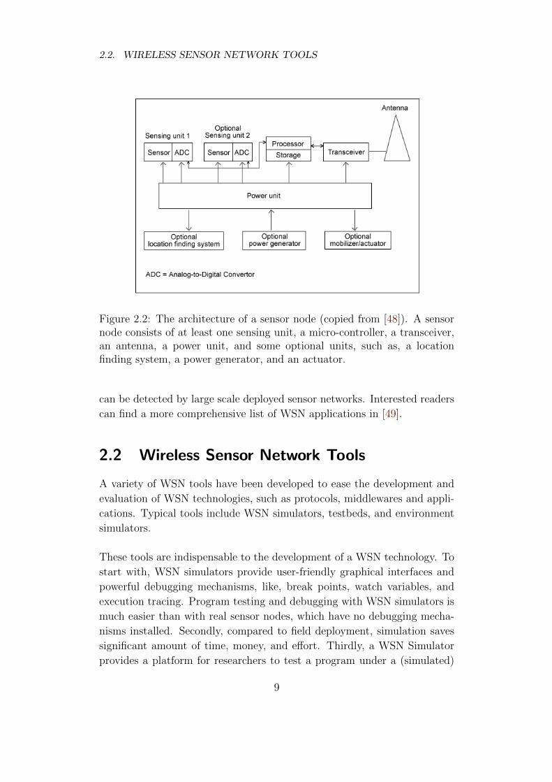
actuator, as depicted in Figure 2.2.
7

CHAPTER 2. BACKGROUND
Figure 2.1: The architecture of a typical Wireless Sensor Network. TheWSN consists of a collection of sensor nodes interconnected by wirelesslinks and is connected to the Internet via a sink or gateway.
Sensor nodes are data sources, while a sink is the entity where the data is
gathered. A sink can be a normal node in the network, an entity outside
the sensor network, or a gateway to another network such as the Internet
[35].
To accomplish their tasks, sensor nodes have to cooperate. Most often,
they communicate via radio. 802.15.4 [33] or IEEE ZigBee [57] is a typical
standard for low data rate and high loss rate radio channels used by WSNs.
Other wireless medium include optical, sound, and inductive medium.
WSNs support a broad spectrum of applications, ranging from vehicle track-
ing to environmental monitoring, from battlefield surveillance to homeland
security, from remote patient monitoring to home automation, and from
habitat monitoring to catastrophe detection. For example, WSNs may be
deployed outdoors to detect toxins and to trace the sources of contamina-
tion. Tiny sensors can be embedded into a patient’s body to continuously
monitor her physical conditions. Volcano eruption, earthquake, and tsunami
8
2.2. WIRELESS SENSOR NETWORK TOOLS
Figure 2.2: The architecture of a sensor node (copied from [48]). A sensornode consists of at least one sensing unit, a micro-controller, a transceiver,an antenna, a power unit, and some optional units, such as, a locationfinding system, a power generator, and an actuator.
can be detected by large scale deployed sensor networks. Interested readers
can find a more comprehensive list of WSN applications in [49].
2.2 Wireless Sensor Network Tools
A variety of WSN tools have been developed to ease the development and
evaluation of WSN technologies, such as protocols, middlewares and appli-
cations. Typical tools include WSN simulators, testbeds, and environment
simulators.
These tools are indispensable to the development of a WSN technology. To
start with, WSN simulators provide user-friendly graphical interfaces and
powerful debugging mechanisms, like, break points, watch variables, and
execution tracing. Program testing and debugging with WSN simulators is
much easier than with real sensor nodes, which have no debugging mecha-
nisms installed. Secondly, compared to field deployment, simulation saves
significant amount of time, money, and effort. Thirdly, a WSN Simulator
provides a platform for researchers to test a program under a (simulated)
9

CHAPTER 2. BACKGROUND
hostile environment. Forth, environment simulators simulate the environ-
ment, provide scenarios for WSN testbeds and simulators. With the help
of environment simulators, we can easily repeat our experiments under the
same scenarios, test our programs under hard-to-obtain scenarios, such as,
an earthquake or a tsunami. Finally, a testbed is more accurate and can
gather real life scenarios for WSN simulators.
2.2.1 Wireless Sensor Network Simulators
A WSN simulator simulates sensor nodes, communication channels and sen-
sor networks by means of software. WSN simulators play an indispensable
role in the early stages of the development of a WSN technology. First, WSN
simulators are often equipped with easy-to-use graphical user interfaces and
powerful debugging mechanisms (e.g. break points, watch variables, and ex-
ecution tracing) to ease and speed up program development. Second, testing
programs by simulation reduces the cost incurred by purchasing real hard-
ware and real world deployment. Third, simulation saves time. Setting up a
simulated environment is much faster than field deployment. Forth, A WSN
simulator can provide a simulated hostile environment, such as, on top of
a volcano or under a deep ocean, for researchers to test their programs. In
contrast, testing programs under such environments in real world is almost
impossible. Finally, in the real world, a scenario is not repeatable. But with
simulation, the experiment can be conducted many times under the same
scenario.
Existing WSN simulators were built with different purposes, hence, work on
different abstraction levels, for different operating systems, and have vary-
ing functionalities. This brings the necessity to classify them. According to
at which level a simulator works, WSN simulators can be classified into four
categories: instruction level, operating system level, network level, and ap-
plication level simulators. No simulator can simulate every level accurately
without any simplifying assumptions due to the difficulties in construction
and the unacceptable computational costs. Existing simulators all have
varying degrees of emphasis on different levels. For example, MSPsim [28] is
a pure instruction-level emulator, which emulates MSP430 microcontroller-
equipped sensor boards, but does not support nodes communications and
mobility. ATEMU [45] and Avrora [51] emulate the operation of individ-
ual sensor nodes equipped with AVR microcontrollers in an instruction by
instruction manner, but simulate the interactions between nodes in a real-
10
2.2. WIRELESS SENSOR NETWORK TOOLS
istic manner. TOSSIM [40] is a simulator dedicated to TinyOS. It captures
TinyOS behavior at a very low level but makes several simplifying assump-
tions in terms of node architecture and radio medium. COOJA [43] is a
simulator for the Contiki [27] operating system. It works on the OS level,
but also provides instruction-level emulation.
As a WSN simulator often makes a variety of simplifying assumptions, this
simplifies the construction of a simulator but, in the meanwhile, incurs
fidelity loss. A program passes the test of a simulator doesn’t guarantee
that it can run in a real environment without errors. This is proved by
[38], which summarizes 6 commonly used assumptions by simulators: (1)
the world is flat; (2) a radio’s transmission area is circular; (3) all radios
have equal range; (4) if I can hear you, you can hear me; (5) if I can
hear you at all, I can hear you perfectly; (6) signal strength is a simple
function of distance. Hence, simulators are only suitable for early stages of
WSN technologies development. The later stages of a development involves
the assessment of the realistic performance, error resilience and other non-
functional properties of the target technology.
2.2.2 Wireless Sensor Network Testbeds
A WSN testbed can provide more accurate evaluation of a target software
over a simulator. WSN testbeds are widely used in the later stages of the
development of a WSN technology. A WSN testbed is a platform deployed
in a controlled environment to support the development and evaluation of
WSN technologies. A WSN testbed usually consists of a moderate number
of real sensor nodes installed with middlewares, protocols, and applications.
Auxiliary hardware and software are provided for debugging and system
management, such as, system-wide reprogramming [30].
The difference between a WSN testbed and a WSN simulator is that the
former employs real sensor nodes and is deployed in a real environment,
whereas, the latter involves no hardware and real world deployment, every-
thing is simulated by software. Compared to a field deployment, a WSN
testbed usually consists of smaller number of nodes, has auxiliary hardware
and software and is sometimes deployed in a different environment (espe-
cially when the real deploy environment is hard to obtain or access). A WSN
testbed confines the number of sensor nodes to a degree that the debugging,
sensor nodes reprogramming, and other system analysis can be conducted in
a controlled and efficient way. A WSN testbed often incorporates hardware
11

CHAPTER 2. BACKGROUND
and software facilities to enable program debugging, node reprogramming,
and scenario simulation etc. A WSN testbed cannot root out the problem
of realistic program testing, because, its deployment environment is often
different from that of the real sensor network.
The following are some example WSN testbeds. MoteLab [56] is an open
source WSN testbed developed by Harvard University. Users can upload
and dispatch jobs to the sensor nodes in the testbed and download results
through an easy-to-use web-based interface. TWIST [30] is a scalable and
reconfigurable indoor WSN testbed. In addition to traditional testbed ser-
vices, it also provides several novel features: incorporating heterogeneous
node platforms into one experiment, active control of node power supply,
and supporting both flat and hierarchical sensor networks. Sensei-UU [46]
is a WSN testbed that supports mobile sensor nodes. It utilizes robot tech-
nology to localize mobile nodes.
2.2.3 Environment Simulators
An environment simulator is a simulator that simulates one or more facets
of a deployment environment of a WSN. It outputs the changes of the status
of the simulated object. For example, a fire simulator [4] can simulate the
trend and temperature of a large wild forest fire. Volcano simulators [16]
simulate the eruption of a volcano. Ocean wave simulators [31] simulate the
direction and strength of ocean waves. Earthquake simulators [5] simulate
the changes of related environmental factors during an earthquake. Mobility
simulators generate position changes of nodes over time. The generated
scenario information can be used as input of a WSN simulator or a testbed
to test the performance of a target technology under certain scenarios.
2.3 WiseML
Having decided the content of the standard configuration file, the next step
is to choose an appropriate configuration language to describe the config-
uration file. A desired configuration language should satisfy the following
requirements: (1) Ease of use. This can always be a criterion to evaluate
a programming language. No one would refuse a language whose syntax
is unambiguous and close to natural language. (2) Flexibility and exten-
sibility. These two properties appear especially important in the case of
12

2.3. WISEML
WSN tools integration. Since the number and type of simulation parame-
ters and results approximate to innumerable, and are subject to change, a
language that allows its users to define, add, remove, or modify configura-
tion parameters freely gains favor. (3) Supported by major programming
languages. If a configuration language is not supported by popular program-
ming languages (e.g., C/C++ and Java), then parsing and storing data can
be very challenging. Supportive libraries or packages of a programming lan-
guage can significantly simplify the process of configuration file processing.
(4) Platform independent. Simulators are usually written in different lan-
guages, work on heterogeneous software and hardware platforms. For the
ease of information exchange, configuration files should be independent of
platforms.
WiseML [22], standing for WIreless SEnsor network Markup Language,
meets all the requirements stated above and is the configuration language
used to describe the Common Input and Output format. There are still
other WSN simulators that support WiseML, such as, Shawn [39] and WS-
NGE [34]. WiseML is defined by the WISEBED project. It is an XML
(eXtensible Markup Language) [17] based language confined by WiseML
schema [23]. It inherits all the properties of XML. For example, WiseML
data is stored in plain text format, which makes it platform independent;
Almost all of the major programming languages provide support for XML,
hence, WiseML; XML enables its users to define their own tags and syntax
with ease. This makes WiseML a highly flexible and extensible language, in
that, the only thing to change to modify it is the WiseML schema. WiseML
also have the advantage of the ease of use of markup languages. However,
WiseML also has its weakness. It assumes there are common node types
and applications. However, in fact, it is extremely difficult to find out a
node type or an application supported by all WSN tools. The format of a
WiseML file is not optimal for implementation. For example, the scenario
section could use a hierarchical structure to make the implemented system
more efficient (See Chapter 6.2.3 for a detailed explanation).
A configuration file written in WiseML is called a WiseML file. The WiseML
schema defines that a WiseML file should contain both input and output
data common to WSN tools. A WiseML file consists of three sections: the
setup section (static input), the scenario section (dynamic input), and the
trace section (output). The setup section contains the static information
relating to the simulation as a whole (e.g., the duration of a simulation,
the coordinate type of a WSN etc.), the node properties (e.g., position,
13

CHAPTER 2. BACKGROUND
node type, etc.), as well as link properties (e.g., encrypted, rssi, etc.). The
scenario section specifies the dynamic changes of the nodes’ and links’ prop-
erties during the simulation. It describes, for example, at which time a node
or a link fails and at which time a node moves. The scenario information
can be obtained from a user’s manual input, from an environment simula-
tor, or from a testbed. Unlike the first two sections, the trace section is
used to store simulation results. It records the sensor readings and topol-
ogy changes and so on in chronological order. A file written in WiseML is
supposed to has an extension of .wiseml. Please refer to Appendix A for an
example WiseML file generated by COOJA.
2.4 COOJA
COOJA [42] is a discrete event WSN simulator to which I added WiseML
support. It is a WSN simulator dedicated to the Contiki OS [27]. It fea-
tures cross-level, cross-platform simulation, deployable code simulation, and
extensibility. It supports five different types of motes working on three dif-
ferent levels (instruction level, OS level, and application level). Deployable
code (the code running on a real sensor node) can be compiled by COOJA
into a simulation, which makes it much easier to compare, between COOJA
and testbeds, the execution results of deployable codes. COOJA is platform
independent because of its programming language - JAVA. Extensibility is
achieved by the deployment of plugins and interfaces. Plugins are inde-
pendent programs that add new functions to COOJA. They interact with
the current simulation and extend the power of COOJA. Plugins can be
added to or removed from COOJA with ease. Sensor node properties, such
as, position, temperature sensor, humidity sensor, etc., are implemented as
interfaces. Interfaces of a node can also be added or removed. This gives
COOJA flexibility and extensibility. Figure 2.3 is captured from COOJA.
The GUI consists of four windows (which correspond to four plugins) – the
control panel, the visualizer, the log listener, and the timeline window. In
this simulation, five contiki nodes and five sky nodes are running simultane-
ously, they are distinguished by color managed by the mote type interface.
The numbers to the right of each node are their positions managed by the
position interface, and the colored rectangle piles to the left of each node
represent LEDs equipped by each node, they are managed by the LED
interface.
14

2.4. COOJA
Figure 2.3: The COOJA simulator screenshot. Four sub-windows corre-spond to four plugins: the control panel, the visualizer, the log listener, andthe timeline. Sensor nodes with their positions and LEDs are visualized inthe visualizer.
COOJA stores its configuration information into an XML file with an exten-
sion of .csc. This configuration file contains information with regard to each
node and link (e.g., node types, node interfaces, positions, and link prop-
erties etc.) and information regarding the whole simulation, such as, the
plugins used in one simulation. Please refer to example.csc in Appendix A
for an example.
15


Chapter 3
Related Work
Some efforts have been made during the past decade to integrate existing
WSN tools with various motivations. Previous work mainly focused on one
of the following aspects: the unification of WSN simulators, the integra-
tion of WSN testbeds, the coupling of environment simulators with WSN
simulators and testbeds or the integration of different types of WSN tools.
COOJA [43] integrates multiple WSN simulators by unifying their source
codes. It integrates two instruction level emulators – MSPsim [41] and
Avrora [12] into its own simulation framework. MSPsim is an emulator
for MSP430 [8] microcontroller-equipped sensor boards, and Avrora is an
emulator for AVR [1] microcontroller-equipped boards. By integrating in-
struction level emulators, COOJA is able to simulate on three different
levels: instruction level, OS level, and application level.
MiXim [36] combines and extends several OMNeT++ [10] based WSN sim-
ulators. It incorporates the mobility and connectivity functionalities of the
Mobility Framework (MF) [26], radio propagation models of CHannel SIM-
ulator (ChSim) [53], and the protocol libraries of the MAC simulator [7], the
Positif framework [11], and the Mobility Framework. The base of MiXiM
supports environment models, nodes connectivity and mobility, signal re-
ception and collision, experiment setup, and a protocol library containing
a rich set of communication protocols. MiXiM also introduces a number of
extensions to enrich its functionalities. The full support of 3D, models for
walls and obstacles, different frequencies and transmission media, to name
but a few.
Park et al. [44] integrated a network level simulator (SensorSim) with a
17
CHAPTER 3. RELATED WORK
node level simulator (ESyPS) via the tight integration approach. The node
level simulator is capable of providing power profiling for each running task
as well as detailed power statistics for the CPU, radio, sensors, and other
peripherals of a sensor node. And the network simulator features support-
ing a number of communication protocols, noise models, realistic scenarios
simulation, and target tracking. By combining these two simulators, the
authors can obtain more precise estimation of the energy consumption of a
sensor node or a task in a sensor network under a specific scenario.
Work [43], [36], and [44] stated above integrate multiple tools into one
by unifying their source codes. This technique is classified as the tight
integration approach according to the taxonomy presented in Chapter 4.1.
This integration approach can only be applied to the simulators written in
the same programming language. This requirement limits the number and
type of simulators that can be integrated.
Bonnmotion [52] integrates itself with a number of other WSN or network
simulators by supporting multiple output formats. These formats are ob-
tained by offline translations. This integration approach is classified as the
simple offline loose integration approach in Chapter 4.1. Bonnmotion is a
mobility scenario generation and analysis tool. It provides mobility sce-
narios for WSN or network simulators. The current version supports five
mobility models: the Random Waypoint model, the Gauss-Markov model,
the Manhattan Grid model, the Reference Point Group Mobility model,
and the Disaster Area model. The generated scenario can be used with
multiple simulators, including ns-2 [9], GloMoSim/QualNet [25], COOJA,
and MiXiM.
NetTopo [47] integrates simulation and real sensing from a testbed into
one framework. Simulated sensor nodes and real nodes of a testbed are
incorporated into one virtual WSN, and communicate with each other. The
integrated testbed provides real-life scenario to the simulation, and validates
the target technology in a realistic and accurate manner. On the other hand,
the simulator enables large-scale WSN simulation with little cost. This
solution effectively attacks the monetary problem related with large-scale
deployed WSN testbeds and the inaccurate problem incurred by simulation.
Sridharan et al. [50] combined a structural simulator with a WSN simulator
(TOSSIM [40]). The structural simulator is used to generate the responses
18

of a building to external forces, the computer generated scenario data is then
input into TOSSIM to validate a structural health monitoring algorithm.
FireSenseTB [37] integrates a fire simulator with a WSN testbed. The fire
simulator is used to generate fire scenario for the testbed, and the testbed is
then used to validate an fire detection algorithm. This approach gets rid of
the bureaucracy and unrepeatability problems caused by setting up a real
forest fire, and the inaccuracy problem caused by simulation.
Work [47], [50], and [37] described above use the smart online loose in-
tegration approach defined in Chapter 4.1 to integrate various tools into
one. Compared to other approaches, this approach is more advanced and
sophisticated.
Abdolrazaghi’s work [24] has many similarities with this one, in that it also
tries to define a standard configuration file format to eliminate the com-
munication barriers among different WSN tools. But the method used by
Abdolrazaghi requires a configuration file containing every possible param-
eter used by WSN simulators. However [54] argues that this method is not
feasible because the number of configuration parameters to be included is
numerous. The integration approach used by work [24] is the simple of-
fline all-embracing loose integration approach according to the taxonomy
provided in Chapter 4.1.
WISEBED [29] has the closest relation with this work. It focuses on testbed
integration, but also aims at providing traces of data from the physical envi-
ronment and deriving models of real-life scenarios for simulation. To serve
the latter purpose, the WISEBED group defined a configuration file for-
mat, the WiseML format, for WSN simulators and testbeds. The WiseML
format contains both input and output data common to WSN tools. The
WiseML format is fully in compliance with the Common Input and Output
format. Therefore, it is directly adopted as a concrete representation of
the CIO format proposed by this work. The integration approach used by
this work is the simple offline CIO loose integration approach according to
Chapter 4.1.
19


Chapter 4
Design
In this chapter, I first present and compare a number of integration ap-
proaches and give a unique taxonomy for them. Next, I describe the data
structure used by wisemlCooja – a bidirectional online WiseML converter
for COOJA. Finally, I elaborate the functional structure of wisemlCooja.
4.1 Integration Approaches
As discussed in Chapter 1.1, to meet the requirements of the development
of a WSN technology, WSN tools must cooperate. I investigated into a
number of possible integration approaches, and classified them as follows.
According to the tightness of the integration, integration approaches can be
classified into tight integration and loose integration. Tight integration
refers to joining existing simulators’ source codes tightly and locally to form
a new inseparable simulator. After this integration, each participating sim-
ulator will loose its independent format, and become a component of the
new simulator. Successful examples are COOJA [43], which incorporates
MSPsim [28] and Avrora [51] emulators into one simulation framework, and
MiXiM [36], which joins and extends the Mobility Framework (MF) [26], the
CHannel SIMulator (ChSim) [53], the MAC simulator [7], and the Positif
framework [11]. However, tight integration can only be applied to simula-
tors written in the same programming language, which limits the number
and type of simulators that can be integrated. Loose integration employs
a medium to bridge the differences among different WSN tools. The most
21

CHAPTER 4. DESIGN
common medium is a standard configuration file supported by each WSN
tool. Loose integration can be further categorized according to three clas-
sification criteria stated as follows.
Criteria 1: The degree of automation
According to how much human effort is involved in a cooperation, loose
integration approaches can be classified into two categories.
Category 1: Simple loose integration As suggested by its name, it
is a very simple approach in the sense that the interaction among WSN
tools is performed by users instead of programs. A user has to prepare
the configuration file for one tool, and then transfer it to another locally
or remotely by traditional file transfer methods, such as, email attachment
and USB flash disk copy.
Category 2: Smart loose integration
Smart loose integration refers to loosely connecting WSN tools into a fed-
eration. This is usually achieved by adding intermediary software to tie dif-
ferent tools into a virtual tool. Different tools can reside on the same host.
These tools are then interconnected by local glue software (local smart ap-
proach). Or they can be installed on geographically distributed hosts and
are connected over the Internet by network sockets or webservices (network
smart approach). The result virtual tool usually has a unified GUI. A user
interacts with the GUI to set configuration parameters and get results. The
system will automatically send user input to appropriate tools and return
desired results to the user. We have noticed some effort [47], [50], and [37]
on the local smart approach, but to the best knowledge of the author, no
attempt at the network smart approach.
Criteria 2: The content of the standard configuration file
What hampers the cooperation among WSN tools is the incompatibility
of their configuration file formats. This calls for a standard configuration
file format supported by every WSN tool. According to what should be
included in this standard configuration file, loose integration approaches
can be classified into the following two categories.
Category 1: All-embracing configuration file format
Started out with the best wishes, researchers expected that an all-embracing
configuration file encompassing every input parameter required by and out-
put data resulted from any tool can bridge the differences among WSN
22

4.1. INTEGRATION APPROACHES
tools, hence, eliminate the barrier of collaboration. Some special programs
called translators were expected to translate the standard configuration files
to or from a tool’s native configuration files, so as to minimize the changes
to existing tools. This approach was partially evaluated by Abdolrazaghi
[24]. Due to the sheer number of possible input and output data, Abdol-
razaghi only evaluated a small number of input data on a few WSN simula-
tors. Translators were built to translate unidirectionally from the standard
configuration file format to a tool’s native format. Even if with such great
simplification, the implementation was still very tough. Practice and theory
[54] both proved that this approach is not feasible because it is impossible
to enumerate every possible input and output data.
Category 2: Common Input and Output configuration file format
The problem of the all-embracing configuration file approach lies in that the
amount of information that is tried to embrace into the standard configu-
ration file is unlimited. To attack this problem, the easiest way is to reduce
the quantity of information. Consider that, tools have different purposes,
some input or output data are only specific to one tool, it is not necessary
to include every such kind of specific information into the standard config-
uration file. Only input and output data common to WSN tools are needed
to be included into the standard file, tool specific information can be saved
into another separate file. This approach effectively keeps the quantity of
information in the standard configuration file within an acceptable limit.
Criteria 3: Concurrency
According to if cooperating WSN tools can execute simultaneously and
interact with each other at run-time, loose integration approaches can be
classified into another two categories.
Category 1: Offline integration
This approach only allows at most one tool to execute at a time. One tool
must wait until the whole data set required is generated and saved into a
configuration file by another.
Category 2: Online integration
This approach allows multiple WSN tools run simultaneously. A tool can
consume the data generated by other tools before the whole data set is
produced.
After compared the strengths and weaknesses of each approach and took
the time constraint into account, I decided to adopt the simple offline CIO
23

CHAPTER 4. DESIGN
loose integration approach. Within the context of this thesis, this name is
briefly referred to as the Common Input and Output integration approach
or the CIO integration approach.
4.2 Data structure design
The Common Input and Output integration approach is based on the as-
sumption that there must be a set of input and output data that is common
to WSN tools. It requires that the standard configuration file should only
contain the common input and output data, tool specific data should be
saved into another file. Hence, it is necessary to split the configuration data
into two portions, with one portion containing the common input and out-
put data and another containing tool specific data. In the case of COOJA,
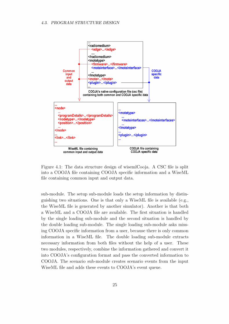
I divided COOJA’s native CSC configuration file (Appendix A file one) into
a WiseML file (Appendix A file two) and a COOJA file (Appendix A file
three). The COOJA file contains COOJA specific information, such as,
plugins and interfaces. The WiseML file stores the common input and out-
put data, such as, node types and node positions. Figure 4.1 depicts the
relations among these three files.
4.3 Program structure design
Based on the modular programing theory, I divided the functionalities of
wisemlCooja into three modules: (1) the loading model, which converts the
WiseML format into COOJA’s native format; (2) the saving model, which
converts COOJA’s native format into WiseML format; and (3) the scenario
generation model, which converts text format testbed temperature logs into
WiseML format scenarios. The advantages of this program structure are
ease of implementation, errors being confined within a single module, and
code reuse. The structure is shown in Figure 4.2.
The left branch of Figure 4.2 shows the structure of the saving model.
The saving module splits COOJA’s configuration file into COOJA specific
information and common information and saves them into a COOJA file (by
the .cooja sub-module) and a WiseML file (by the .wiseml sub-module).
The right branch of Figure 4.2 presents the structure of the loading mod-
ule. It comprises two sub-modules: the setup sub-module and the scenario
24
4.3. PROGRAM STRUCTURE DESIGN
Figure 4.1: The data structure design of wisemlCooja. A CSC file is splitinto a COOJA file containing COOJA specific information and a WiseMLfile containing common input and output data.
sub-module. The setup sub-module loads the setup information by distin-
guishing two situations. One is that only a WiseML file is available (e.g.,
the WiseML file is generated by another simulator). Another is that both
a WiseML and a COOJA file are available. The first situation is handled
by the single loading sub-module and the second situation is handled by
the double loading sub-module. The single loading sub-module asks miss-
ing COOJA specific information from a user, because there is only common
information in a WiseML file. The double loading sub-module extracts
necessary information from both files without the help of a user. These
two modules, respectively, combine the information gathered and convert it
into COOJA’s configuration format and pass the converted information to
COOJA. The scenario sub-module creates scenario events from the input
WiseML file and adds these events to COOJA’s event queue.
25

CHAPTER 4. DESIGN
Figure 4.2: The functional structure of wisemlCooja. It comprises threemodules: the loading module, the saving module, and the scenario buildingmodule.
26

Chapter 5
Implementation
In this chapter, I discuss the core issues with respect to the implementation
of the wisemlCooja. I first present a series of key implementation deci-
sions. Next, some essential assisting internal and external data structures
are discussed. Finally, I describe the package structure of wisemlCooja.
5.1 Implementation decisions
During the implementation, a series of decisions were needed to be made
for various reasons. In the following, some important decisions are listed.
5.1.1 Adaptation v.s. Converter
There are two possible approaches to make COOJA support WiseML. One
is to adapt COOJA’s source code directly, let it accept WiseML as its sole
input and output format. The original COOJA configuration file format
is replaced by WiseML. Another is to build a converter in the form of
a COOJA plugin. The converter converts between WiseML format and
COOJA’s native configuration format on-the-fly. The latter approach allows
for the coexisting of both WiseML and COOJA’s native format.
The advantages of adaptation are that it can make use of COOJA’s existing
code to the largest extent and that it has better performance. The reason
is that it modifies COOJA from inside, hence, reduces method invocations
and saves time and space. The disadvantage of this approach is that the
adaptation of COOJA may interfere with other updates. That is, COOJA is
27
CHAPTER 5. IMPLEMENTATION
an open source software, it is updated at a high frequency, the adaptation
in question can be paralleled with other updates to COOJA. It is very
likely that on the completion of the adaptation, we will find that we will
have implemented the proposed approach on an older version of COOJA.
Further more, COOJA is a well established system with a considerable
extent of complexity, modifying it from the core can be very complicated
and error-prone.
A converter adds extra converting time to the original loading and saving
process. But it is simple, independent and clean. It does not interferes
with other updates of COOJA and does not have the danger of system
collapse caused by changing COOJA’s source code. As a result, I choose
this approach.
5.1.2 Interaction with COOJA
Having decided to develop a converter, the next step is to decide how to
exchange information between COOJA and this converter. There are two
choices: (1) invoking multiple low level methods provided by COOJA di-
rectly; (2) invoking one high level COOJA method, which is responsible to
interact with the low level methods in choice 1. The first choice involves
less method invocations and is hence more efficient. But it requires the
knowledge of COOJA’s low level techniques, hence, more complicated and
error-prone. The second choice is the opposite. It takes slightly more execu-
tion time and space, but significantly simplifies the implementation. Thus,
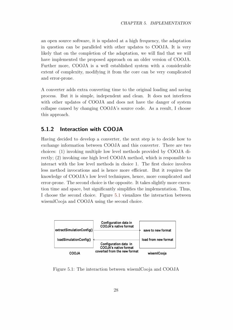
I choose the second choice. Figure 5.1 visualizes the interaction between
wisemlCooja and COOJA using the second choice.
Figure 5.1: The interaction between wisemlCooja and COOJA
28

5.1. IMPLEMENTATION DECISIONS
5.1.3 Assumptions regarding WiseML schema
I make some assumptions regarding the WiseML schema while I am im-
plementing wisemlCooja, because the definition of the WiseML schema has
not been finalized at the time of implementation.
Assumption one: WiseML schema requires that each sensor node should
have a node type associated with it, but it doesn’t specify how to name
different node types. In this implementation, two kinds of node types are
distinguished: the common node types, which are commonly used by WSN
tools, and the tool specific node types, which are only supported by one
or a few tools. I defined a number of node types as standard node types
and assigned them specific names. These standard node types are referred
directly by their names in a WiseML file. For simulator specific node types,
I use the following format:
LLL : simulator’s name : simulator specific node type : other help
info
This format always starts with three capitalized letters (LLL) to distinguish
them from standard node type names. Colons (:) are used to separate each
item of the compound name. The second field is the name of a simulator,
which supports the specific node type. The third field is the node type’s
name used by this simulator. And the last field is an optional field, which
is used to save some help information to ease the implementation.
A simulator supporting WiseML should be able to distinguish common node
types from simulator specific node types by examining the format of the
node type name. If it starts with LLL, then the simulator should go on and
examine the second field to see if it is its own name. If yes, it can simulate
this node, otherwise, it can either ignore this node or choose another type
of node to simulate.
Assumption two: Since one simulation can include multiple scenarios, it
is necessary to assign each scenario an ID. The WiseML schema doesn’t
specify the format of scenario IDs, therefore, I assume scenario IDs are
simply serial numbers.
29

CHAPTER 5. IMPLEMENTATION
5.2 Assisting data structures
I classify the data used by wisemlCooja into two categories: internal data
and external data. As suggested by its name, external data are saved on the
second storage in the form of files. The external files have various usages:
maintaining a relationship between the WiseML format and COOJA’s na-
tive format or maintaining a list of recently opened files. Internal data are
constructed at run-time, they only reside in memory. Internal data are used
to maintain various relations between the WiseML and CSC files.
5.2.1 Internal assisting data structures
In this sub-section, I present the most important internal data structures
used by wisemlCooja. They are described in a structured way: ”Name”
is the name of a JAVA data structure used by wisemlCooja. ”Data type”
defines the type of this data structure (e.g. a list, a tree, or a map). ”Data”
describes the content of a data structure. But it only presents the structure
of the content, specific values are not provided. Different entries of data are
embraced in parenthesis and separated by commas.
1. Name: idMap
Data type: HashMap
Data: {(standard node ID 1, COOJA node ID 1), (standard node ID
2, COOJA node ID 2),...}Usage: Used to maintain mapping relations between a standard node
ID and a COOJA node ID.
Description: In a standard configuration file, a wireless communi-
cation link between a pair of sensor nodes is identified by the source
and the destination node IDs as follows:
<link source="urn:wisebed:node:sics:X1"
target="urn:wisebed:node:sics:Y2">
COOJA only accepts the following format:
<edge>
<src>Sky 4</src>
<dest>Sky 1</dest>
<ratio>0.8</ratio>
30

5.2. ASSISTING DATA STRUCTURES
<delay>8</delay>
</edge>
Therefore, it is necessary to maintain a mapping relation between a
standard node ID (e.g., urn:wisebed:node:sics:X1 in the above exam-
ple) and a COOJA node ID, which is a serial number (e.g., the last
figures between the <src >and </src >tags in the above example) so
that the loading module of wisemlCooja knows what number should
be assigned to a COOJA’s source or destination node when it tries to
load a simulation from a WiseML file.
2. Name: Relations
Data type: User defined class
Data: {standard node type, corresponding COOJA node type, COOJA
node type identifier, application, {ID1, ID2, ...} (IDi is the ID of a
standard node which has the same node type and application as spec-
ified by fields one and four)}Usage: Used to maintain a mapping relation among a standard node
type and the nodes that belong to this type and the corresponding
COOJA node type.
Description: When wisemlCooja loads a simulation from a single
standard configuration file, all COOJA specific information is missing,
hence, it does not know which COOJA node type should be created
when it encounters a node type in the standard configuration file. The
program asks the user to decide which COOJA node type should be
used, and then saves this mapping relation in this data structure. This
mapping relation is revisited by wisemlCooja when it constructs the
mote type, mote, and edge information for COOJA to load.
3. Name: Node
Data type: User defined class
Data: {node ID, {x, y, z} (node position), {(sensor name 1, reading),
(sensor name 2, reading), ...}}Usage: Used to record a sensor node’s position and sensor readings
at a certain time.
Description: The property values (position, sensor readings, etc.)
of a sensor node at a given time recorded by this data structure can
be used to construct scenario events, which specifies the changes of
31

CHAPTER 5. IMPLEMENTATION
the network (including node property changes), at a certain time, and
then is processed by COOJA in chronological order.
4. Name: Link
Data type: User defined class
Data: (source node ID, destination node ID)
Usage: Used to represent a wireless communication link by its source
and destination sensor nodes.
Description: This data structure is used to identify a link in a sce-
nario event, which then is entered into COOJA’s event queue waiting
for processing.
5. Name: linkRatios
Data type: HashMap
Data: {(Link 1, transmission success ratio 1), (Link 2, transmission
success ratio 2), ...}Usage: Used to keep the transmission success ratio of a link.
Description: The scenario section of a standard configuration file
allows the simulation of link failures. This is achieved by change the
success ratio of a link. In COOJA, if the success ratio of a link is 0,
then nothing can be transmitted via this link, which is equivalent to
disabling this link. However, a disabled link can resume work at a later
time, and it should has the same success ratio as before. Therefore, it
is necessary to keep the success ratios of links when they are disabled
and restore these values when they are enabled. Note that, the Link
used in this data structure is the same as the 4th (Link) data structure.
6. Name: ScenarioEvent
Data type: User defined class
Data: {timestamp, {enabled Link 1, enabled Link 2, ...}, {disabled
Link 1, disabled Link 2, ...}, {Node 1, Node 2, ...}}Usage: Used to record the changes of the network at a certain time.
Description: The information presented in the scenario section of a
standard configuration file is organized in a chronological order. All
the changes of the network (including the changes of node positions,
sensor readings, and disabled and enabled links and nodes, etc.) at a
time is associated with a timestamp. A scenario event is constructed
32

5.2. ASSISTING DATA STRUCTURES
for one timestamp to hold the changes at that time. Note that the
Node and Link used here is the same as the data structure presented
in 3 (Node) and 4 (Link).
5.2.2 External assisting data structures
The external data are also presented in a structural manner. ”File name”
is the name of the disk file. ”File structure” defines the content of the file.
1. File name: node type map.mappings
File structure:
{standard node type 1 = COOJA node type 1
standard node type 2 = COOJA node type 2
...}Usage: Used to return the corresponding COOJA node type when
the standard node type is given, or to return the standard node type
when COOJA node type is provided.
Description: There are many times when we need to know the cor-
responding node type, when either COOJA node type or the standard
node type is known. This file stores the mapping relations between
COOJA node types and standard node types in plain text format for
every standardized node type.
2. File name: node class info.mappings
File structure:
{COOJA node type 1 = COOJA node name : prefix of source or
destination node of a COOJA edge : prefix of COOJA mote type
identifier : interfaces of the COOJA node type : the file extension
of the firmware used on this type of nodes : the target platform of a
compilation : the name of the mote ID interface used by COOJA
COOJA node type 2 = ...
...}Usage: Used to retrieve other COOJA specific information when
COOJA node type is given.
Description: When the system loads a simulation from the new for-
mat, the information in the new format should first be converted into
a format that COOJA understands and then be passed to COOJA to
be loaded. During the conversion, a set of COOJA specific parameters
33

CHAPTER 5. IMPLEMENTATION
are needed. Among these parameters, COOJA node type is compar-
atively easy to obtain, but others are hard to get. Fortunately, there
is a fixed relationship between a COOJA node type and other param-
eters. If we store the relationships into a file, like this one, then we
can get other parameters easily as long as we know the COOJA node
type. These relationships are stored in this file in plain text format.
Different parameters are separated by colons.
3. File name: wisemlhistory.txt
File structure: {X.wiseml ; Y.wiseml ... } (max 10 file names)
Usage: Used to keep a history of recently opened WiseML files.
Description: When a user wants to load a simulation from the new
format, she is asked to select a WiseML file for loading. wisemlhis-
tory.txt records the latest 10 files opened by the user. The latest
opened file is displayed in the file choosing dialog as suggestion so
that the user doesn’t need to go through the complicated file selection
process if she just wants to use the same file as the suggested one.
This eases the selection of configuration files.
5.3 Package Structure
The package structure of wisemlCooja is shown in Figure 5.2.
The wisemlCooja package contains two first level class files – WisemlPro-
cessor.java and ScenarioGenerator.java. The first class is the main class
of this package. It comprises the loading module and the saving module.
The ScenarioGenerator.java class is used to convert text format tempera-
ture values logged by a testbed into WiseML format and insert it to an
existing WiseML file as scenario. The gui package contains all the dialogs
used by the system. They provide user friendly graphical interfaces. Fig-
ure 5.3 shows a dialog displayed when the system tries to load a simulation
from a single WiseML file. As we can see, the information from the stan-
dard configuration file is displayed in the upper area and the lower area is
used to gather user input of COOJA specific information. Note that node
type together with the application running on this type of nodes identify
a unique group of nodes, which is called a mote type in COOJA. In Fig-
ure 5.3 there are 2 ESB nodes executing radio-test.esb. The system will
also create exactly 2 nodes in COOJA with the desired COOJA node type
and application provided by the user.
34

5.3. PACKAGE STRUCTURE
Figure 5.2: The package structure of wisemlCooja. It consists of two firstlevel class files (wisemlProcessor.java is the main class) and a gui sub pack-age, which contains dialogs used to provide a graphical interface to theuser.
35

CHAPTER 5. IMPLEMENTATION
Figure 5.3: A screenshot of wisemlCooja. It was captured when wiseml-Cooja was trying to load a simulation when COOJA specific informationwas not available (only a WiseML file available). The upper area of the di-alog displays the information retrieved from the WiseML file, and the lowerpart is the area for user input.
36

Chapter 6
Evaluation
In this chapter, I evaluate the Common Input and Output integration ap-
proach. After the introduction of the experimental setup in section one. I
present the micro-benchmarks evaluation results in section two. It includes
the size, the space, and the time complexity of wisemlCooja. The last sec-
tion is intended to reveal the evaluation results of the cooperation between
tools.
6.1 Experimental setup
The experiments in this chapter are conducted on a DELL Latitude D630
laptop computer. The operating system used is Windows XP with Service
Pack 3. I use Instant Contiki [6] as the experimental platform, because
it introduces a Linux environment on top of the Windows system and has
most of the required software installed. To use the Instant Contiki virtual
machine, a virtual machine player, called VMware player, is needed. A more
detailed description of the hardware and software used by these experiments
is presented below.
– Hardware –
Model: DELL Latitude D630 Laptop.
CPU: x86 Family 6 Model 15 Stepping 13 GenuineIntel 1995 Mhz
BIOS version: Dell Inc. A13, 2008-7-28
Main memory: 1,024.00 MB
Hard disk capacity: 120 GB
37

CHAPTER 6. EVALUATION
– Operating System –
Windows XP with Service Pack 3
– Other software –
Instant Contiki [6]: A virtual machine, which provides a Ubuntu Linux [14]
8.0 OS environment, on which all the necessary tools for developing contiki
software are installed.
VMware player [15]: A virtual machine player.
The experiments in this chapter are carried out after the stablization of the
system. Each simulation is repeated at least 5 times under the same exper-
imental settings, some exceptionally large or small results are discarded to
eliminate the side effects generated by any temporary interferences irrele-
vant to the target system. When the experiments are being conducted, no
other unrelated applications are running.
WisemlCooja allows loading a simulation from a pair of configuration files
(a WiseML file and its corresponding COOJA file) as well as from a single
WiseML file. Because the various processing time used by these two ap-
proaches have similar patterns, for clarity, the following text only presents
the results of the first situation.
Throughout the remainder of this chapter, several types of files are inten-
sively used: a WiseML file – a configuration file written in WiseML, it con-
tains configuration data commonly used by various WSN tools; a COOJA
file – a configuration file produced by wisemlCooja to collaborate with a
WiseML file, it only contains COOJA specific information; a CSC file –
COOJA’s native configuration file.
6.2 Micro-benchmarks
This section aims at assessing the time and space overheads of the target
system.
COOJA supports five types of motes working on three different levels. The
lower the level a mote works on the more the overheads caused by this type
of motes. Due to the constraint of time and experimental infrastructure,
the system is only evaluated with disturber motes, which work on the ap-
plication level, send out disturbing signals to their neighbors, and require
38

6.2. MICRO-BENCHMARKS
the least resources. The time and space overheads caused by other types of
motes can be examined in future work.
A WiseML file consists of three sections – a setup section, a scenario sec-
tion, and a trace section. These three sections are processed at different
time points. The setup section is the first section to be processed so that
the node and link information can be loaded into the current simulation. Af-
ter the topology of the network is set, wisemlCooja builds scenario events
based on the information in the scenario section and inserts these events
into COOJA’s event queue. When a simulation is started, scenario events
are executed and simulation traces are exported to the trace section of a
WiseML file. Due to the different characteristics of these three sections,
they have to be evaluated separately.
6.2.1 Code size
The size of a program reveals, to some extent, the complexity of the system.
It is worthwhile to assess the size of the wisemlCooja converter. Wiseml-
Cooja converts between the WiseML format and COOJA’s native config-
uration format on the fly. It is written in JAVA. It consists of 7 classes,
among them, 5 are Graphical User Interfaces (GUI) handlers. The size of
wisemlCooja is 137.6 KB with the main class WisemlProcessor.java 82.9
KB, accounting for approximately 62 percent of the total size (Figure 6.1).
11 COOJA classes and 54 standard classes are imported into the converter.
Figure 6.1: wisemlCooja’s components and their proportions
39
CHAPTER 6. EVALUATION
6.2.2 Space complexity
The size of a WiseML file affects, to some extent, the viability of the CIO
integration approach. It is essential to know the sizes of WiseML files and
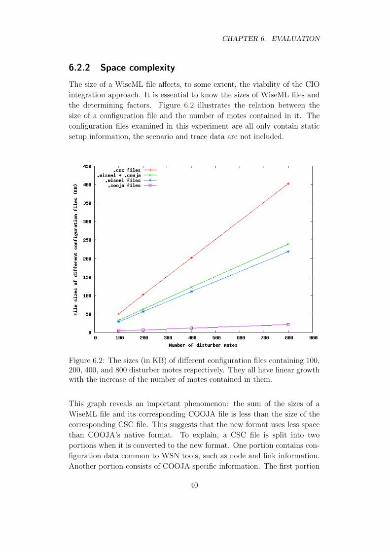
the determining factors. Figure 6.2 illustrates the relation between the
size of a configuration file and the number of motes contained in it. The
configuration files examined in this experiment are all only contain static
setup information, the scenario and trace data are not included.
Figure 6.2: The sizes (in KB) of different configuration files containing 100,200, 400, and 800 disturber motes respectively. They all have linear growthwith the increase of the number of motes contained in them.
This graph reveals an important phenomenon: the sum of the sizes of a
WiseML file and its corresponding COOJA file is less than the size of the
corresponding CSC file. This suggests that the new format uses less space
than COOJA’s native format. To explain, a CSC file is split into two
portions when it is converted to the new format. One portion contains con-
figuration data common to WSN tools, such as node and link information.
Another portion consists of COOJA specific information. The first portion
40

6.2. MICRO-BENCHMARKS
is transformed into WiseML format and stored into a WiseML file. And the
second portion is stored into a COOJA file without any change. Because
WiseML uses a more concise and compact way to describe nodes and links,
the same information takes up less space when it is presented in WiseML.
Therefore, we can conclude that WiseML is an efficient topology description
language. We can also observe that, the sizes of all of these files increase
linearly with the increase of the number of nodes contained in them. In
particular, the sizes of CSC and WiseML files double with the double of the
number of motes contained in them.
A setup only configuration file containing 100 disturber motes has a size of
26.0 KB. If it is expanded with a scenario, which updates nodes’ positions
once per second for 5 minutes, its size becomes 3.8 MB – 1462 times of
the setup only configuration file. If we simulate for 5 minutes and enable
trace exporting while simulation, then after 5 minutes, the file doubles its
size to 7.6 MB. Therefore, scenario and trace account for the majority of a
WiseML file. As we have noticed, the number of motes is the only variable
that determines the size of the setup section. However, the size of the
scenario section is determined by multiple factors, including, the number of
motes, the frequency of scenario events, and the duration of the scenario.
The size of the trace section is determined by the number of motes, the trace
recording frequency, and the exporting duration. In other words, there is
no upper limit for the size of a WiseML file, it is only determined by the
requirement of the application. It is not uncommon that we have a WiseML
file of Giga bytes.
6.2.3 Time complexity
The time used to process WiseML files, such as, loading, saving, scenario
events building, simulating and trace exporting, also plays an important
role in determining the viability of the CIO approach. To time various op-
erations, some statements are inserted into the source code of wisemlCooja
and COOJA. The results are presented below. The conclusions drawn be-
low are based on the assumption that the experimental setup, including
hardware and software, is given.
The loading operation (new format) can be divided into three steps: (1)
Loading the configuration files into memory; (2) Converting WiseML format
to COOJA’s native format; and (3) Creating the simulation. The time used
by the first step is determined by the sizes of the pair of configuration files
41

CHAPTER 6. EVALUATION
(WiseML and COOJA files) to be loaded. The time used by the second
and the third steps, in theory, are only determined by the number of motes
contained in a WiseML file. However, in practice, the time used by these
steps increases with the size of the WiseML file as a whole even if the number
of motes contained in this file does not change. This is because the sizes
of the memory or the caches of the computer confine the number of data
can be loaded into them. When the size of a file exceeds the threshold, the
file has to be split into many parts and different parts have to be swapped
between memory and cache or disk and memory. Please note that this kind
of time overheads are caused by the architecture of the computer, instead of
WiseML or wisemlCooja. Figure 6.3 depicts how the time used by various
operations are affected by the number of motes contained in a configuration
file.
Figure 6.3: Mean loading time (in ms) of different configuration files con-taining 100, 200, 400, and 800 disturber motes respectively. The WiseMLconverter performs well when the number of motes exceeds 400 in a config-uration file.
The gap between the mean total loading time of the new and the old formats
42
6.2. MICRO-BENCHMARKS
is mainly caused by the format conversion operation, because loading from
the old format only involves loading the configuration file into memory and
creating the simulation, but loading from the new format needs an extra
operation – format conversion. The total loading time of the old and new
formats both experience slow increases when the number of motes in a
configuration file does not exceed 200. However, when the number of motes
exceeds the threshold, the loading time of both formats increase faster.
COOJA’s processing time has similar increase pattern as the total loading
time of the new and old formats. But the WiseML converting time follows a
different increase pattern. When the number of motes in a configuration file
is less than or equal to 400, the converting time experiences a sharp linear
increase. After the 400 threshold is exceeded, the increase slows down.
Converting a 800-mote configuration file only takes 79 milliseconds more
than converting a 400-mote file. This suggests that the converter performs
well when loads large scale network simulations.
The saving operation (new format) can also be divided into three steps:
(1) extracting configuration data from current simulation as old format; (2)
converting the old format to WiseML format; and (3) saving configuration
files to the second storage. The time used by the third step is affected by the
size of the pair of configuration files (WiseML and COOJA files) to be saved.
Similarly, the time used by the first and the second steps, theoretically, are
only determined by the number of motes contained in a configuration file. In
reality, the time overheads caused by these steps increase with the increase
of a WiseML file even if the number of motes contained in it does not change.
Figure 6.4 illustrates how the time used by various saving operations are
affected by the number of motes in a configuration file.
The difference between the total saving time of the new format and the
old format is largely caused by the format conversion operation. Saving
as old format only consists of configuration data extraction and saving to
disk operations, format conversion is not necessary. The various processing
time used by saving increase near-linearly with the increase of the number
of motes in a configuration file.
If noticed otherwise, the scenario used in the remainder of this section de-
scribes a mobility scenario where motes move according to the Random
Waypoint model. Motes’ positions are updated once per second for 5 min-
utes. The trace is obtained by logging the nodes’ movement for 5 minutes.
43
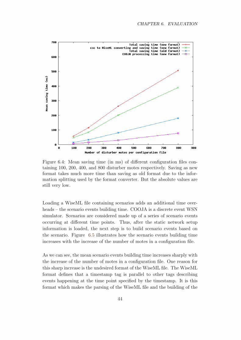
CHAPTER 6. EVALUATION
Figure 6.4: Mean saving time (in ms) of different configuration files con-taining 100, 200, 400, and 800 disturber motes respectively. Saving as newformat takes much more time than saving as old format due to the infor-mation splitting used by the format converter. But the absolute values arestill very low.
Loading a WiseML file containing scenarios adds an additional time over-
heads – the scenario events building time. COOJA is a discrete event WSN
simulator. Scenarios are considered made up of a series of scenario events
occurring at different time points. Thus, after the static network setup
information is loaded, the next step is to build scenario events based on
the scenario. Figure 6.5 illustrates how the scenario events building time
increases with the increase of the number of motes in a configuration file.
As we can see, the mean scenario events building time increases sharply with
the increase of the number of motes in a configuration file. One reason for
this sharp increase is the undesired format of the WiseML file. The WiseML
format defines that a timestamp tag is parallel to other tags describing
events happening at the time point specified by the timestamp. It is this
format which makes the parsing of the WiseML file and the building of the
44

6.2. MICRO-BENCHMARKS
Figure 6.5: Mean scenario events building time (in ms) of different configu-ration files containing 100, 200, 400, and 800 disturber motes respectively.The scenario building time increases sharply with the increase of the numberof motes in a configuration file.
scenario events from this file more complicated. If the WiseML file used
a nested format for the timestamp and its corresponding event tags, the
scenario building process would be pretty much simplified and take much
less time.
Next, let’s take a look at the simulation time of various sized network (Fig-
ure 6.6). The simulated networks comprise 100, 200, 400, and 800 disturber
motes respectively. Each corresponding configuration file can be attached
with a scenario. Simulation times are counted in three different ways: (1)
the time used on static simulation; (2) the time used on simulation with
scenario processing; and (3) the time used on simulation with scenario and
trace processing.
As we can see, with the increase of the number of motes in a configuration
file, all three kinds of simulation have dramatic time increase. Enabling
scenario simulation adds 9% to 11% overheads to static simulation for each
45

CHAPTER 6. EVALUATION
Figure 6.6: The time used by a 5-minute static or dynamic simulation withdifferent sized networks. The simulation time increases dramatically withthe increase of the network scale. Scenario processing adds no more than11% overhead to static simulation, and trace exporting adds up to 10%overhead to scenario enabled simulation.
different sized configuration file. Adding trace exporting can add from 2%
to 10% overheads to dynamic simulations. Trace exporting accounts for 3%
to 9% of the total simulation time (a simulation with scenario and trace
processing). The gaps between the simulation time of the scenario-only and
the scenario-and-trace-enabled simulations are the trace exporting times.
To give the reader a clearer picture, I plot the trace exporting time in a
separate figure (Figure 6.7).
The trace exporting time experiences sharp increase when the number of
motes in a configuration file is less than or equal to 400. When this threshold
is exceeded, the increase slows down.
6.2.4 Conclusion
In conclusion, wisemlCooja is a lightweight (137.6 KB) converter. The size
of a WiseML file only containing the setup section increases linearly with
the increase of the number of motes contained in it. The sizes of the scenario
46

6.3. COOPERATION EVALUATION
Figure 6.7: The trace exporting time of a 5-minute dynamic simulation withdifferent sized networks.
and trace sections depend on specific simulation requirements. The format
converting time used by loading and saving operations, in theory, are only
determined by the number of motes in a network, but in reality, they also
increase with the increase of the size of a WiseML file even if the number of
motes contained in it does not change. They increase near-linearly with the
increase of the network size. Scenario building time increases dramatically
with the increase of the network scale, when the scenario is given. The
simulation and trace exporting time are determined by the network scale,
the scenario events update frequency, the trace exporting frequency and the
required number of simulated seconds.
6.3 Cooperation evaluation
This section tests if by supporting the WiseML format, different tools can
cooperate.
47

CHAPTER 6. EVALUATION
6.3.1 Validation of COOJA generated WiseML files
This subsection aims at validating COOJA generated WiseML files against
the WiseML schema using a validation program.
A WiseML file is an XML file. If a WiseML file is in compliance with XML
syntax, it is well formed. If a WiseML file is not only in compliance with
XML syntax but also conforms to the rules of an XML schema, then it is
valid. [20] lists the XML syntax rules used to validate a well formed XML
file. I use the Linux command xmllint [21] to check the validity of the
WiseML files generated by COOJA. The WiseML files pass the validation
against the wiseml.rng schema.
6.3.2 Cooperating WSN simulators and environment sim-
ulators
This section tests if COOJA, with the help of WiseML, is able to load a
scenario generated by an environment simulator or more specifically a mo-
bility scenario generator, bonnmotion [52], and evaluates the performance
of the cooperation.
Bonnmotion is a mobility scenario generation and analysis tool developed
by University Bonn, Germany. It is the official motion generator used in the
European project Cooperating Object Network of Excellence [3]. The latest
version of bonnmotion supports 5 mobility models: the Random Waypoint
model, the Gauss-Markov model, the Manhattan Grid model, the Reference
Point Group Mobility model, and the Disaster Area model [2]. The gener-
ated scenario is stored in a .movements file. Using bonnmotion’s built-in
translators, this native format can be translated into several other formats
that can be used with ns-2 [9], GloMoSim/QualNet [25], MiXiM [36] and
COOJA. Bonnmotion recently added the support to WiseML. A built-in
WiseML translator can translate a .movements file into a .wml file, which
contains scenario information in WiseML format.
To verify the possibility of the cooperation between bonnmotion and COOJA,
I created a simulation with 6 disturber motes and saved the simulation to
sim.wiseml (14.7 KB) and sim.cooja (2.1 KB). The sim.wiseml file only
contains static information, that is the setup section of a WiseML file. To
generate a mobility scenario for these 6 motes, I issue the following com-
mand in a terminal:
48

6.3. COOPERATION EVALUATION
bm -f mov RandomWaypoint -n 6 -d 600 -i 3600
The command above generates a scenario where 6 motes move according to
the RandomWaypoint model for 600 seconds, the scenario data is recorded
after the initial 3600 seconds has past. The scenario is stored into a file
called mov.movements (3 KB). I use the following command to translate
this file into WiseML format:
bm WiseML -f mov -N nodeIDs.txt
A mov.wml (501 KB) file is generated containing the scenario in WiseML
format. Note that, the mov.wml (501 KB) file is much larger than the
corresponding mov.movements (3 KB) file, because the latter is a node by
row file only containing raw data, but the former has descriptive tags in
addition to position information. nodeIDs.txt (1 KB) contains the node
IDs of all the 6 nodes used in the sim.wiseml file. I Inserted the content of
the mov.wml file into the sim.wiseml file, and let COOJA load the expanded
configuration file. Figure 6.8 shows the movement scenario taking effect in
COOJA. Nodes change their positions from time to time as specified by the
scenario. The network topology at simulated seconds 0, 100, and 600 are
shown in pictures (a), (b), and (c), respectively.
Figure 6.8: Bonnmotion generated scenario taking effect in COOJA. (a)network topology at simulated second 0; (b) network topology at simulatedsecond 100; (c) network topology at simulated second 600
6.3.3 Cooperating WSN simulators
This section inspects the possibility of cooperations between WSN simula-
tors. Cooperation means that one simulator can take, as input, a configu-
ration file generated by another simulator, and simulate accordingly. The
49

CHAPTER 6. EVALUATION
first part of this section examines if COOJA is able to load a non-COOJA
generated WiseML file. The second part looks into if COOJA generated
WiseML file can be loaded by another simulator.
WSNGE
This subsection examines if COOJA is able to load a WiseML file generated
by another WSN simulator WSNGE [34].
WSNGE is a flexible and extensible WSN simulator focusing on user-friendliness,
multiple protocols simulation, and online simulation reconfiguration. WS-
NGE released its support to WiseML 2.0 and posted an exported setup-only
configuration file on its website [19].
The WiseML file contains 6 sensor nodes interconnected by 17 links. Figure
6.9 (a) (copied from WSNGE’s website) illustrates the network’s topology
generated by WSNGE, (b) is the screenshot of COOJA after it successfully
loads the WSNGE generated WiseML file. As we can see, the nodes are in
the same positions. Assign each sensor node a node type and an application,
then we can start a simulation with COOJA. If we want to reload the simu-
lation in the future, we can save it as either COOJA’s native configuration
format (CSC) or WiseML format.
Figure 6.9: WSNGE defined network being loaded into COOJA. (a) networktopology presented in WSNGE, copied from its website [19], (b) the samenetwork being loaded into COOJA.
The size of the WSNGE generated WiseML file is 5.1 KB. The mean total
loading time of this file is 541 ms, in which, 109 ms is used on format
50

6.3. COOPERATION EVALUATION
conversion. In other words, by supporting WiseML, COOJA is able to load
a simulation created by another simulator directly at a cost of 109 ms. The
time overhead is considerably low compared to recreate the same simulation
with COOJA manually by a user.
Shawn
This subsection tests if COOJA exported WiseML files can be loaded by
other WSN simulators, in this case, shawn [39].
Shawn features large scale network simulations. To achieve this goal, it
abandons low level emulation of hardware and network, adopts abstract and
exchangeable models (e.g. communication and transmission models) for low
level effects. This significantly speeds up the simulation, and enables itself
to support up to 106 nodes in one simulation.
Figure 6.10 presents the screenshots captured from both shawn (the first
row) and COOJA (the second row) when they are simulating with the same
configuration file generated by COOJA. This configuration file contains a
node movement scenario generated by bonnmotion. The network topologies
at simulated seconds 0, 30, and 60 are shown in Figure 6.10 (a), (b),
and (c), respectively. The shawn screenshots are provided by Christian
Singer (one of the developers of shawn) from Braunschweig University of
technology, Germany. Because shawn and COOJA use different coordinates
to visualize network topologies, the screenshots generated by shawn are
flipped vertically for easy comparison.
6.3.4 Cooperating WSN simulators and testbeds
This section is intended to test COOJA’s ability to load, as scenario, the
log data exported by a testbed.
The testbed consists of one sink node and three sensing nodes. The three
sensing nodes sense temperature and print out values once per second, these
values are logged into log files and are converted to WiseML format temper-
ature scenario after the completion of the experiment. The sensing nodes
broadcast packets at a speed depending on the current temperature. To
be specific, if the temperature is less than or equal to 25 degrees Celcius,
each of the three nodes sends out 2 packets per second, if the temperature
is greater than 25 but less than or equal to 27 degrees, sends out 4 packets
51

CHAPTER 6. EVALUATION
Figure 6.10: Network topology change overtime presented by two differentsimulators. The first row consists of the screenshots of shawn, the secondrow comprises the screenshots of COOJA. The two simulators simulate withthe same configuration file containing the same node movement scenario.(a) The network topology at simulated second 0. (b) The network topologyat simulated second 30. (c) The network topology at simulated second 60.
per second, otherwise, 8 packets per second. The three nodes keep send-
ing out packets at the fixed speed until a whole second has past and new
temperature values are sensed. The sink counts the number of packets it
receives during one second, and prints out the results.
Figure 6.11 depicts the averaged number of packets per second received by
the sink node over time. To ease observation, the moving average technique
is used. Each value of this graph is obtained by averaging over the next
20 actual packet yields. Three different thicknesses are used to distinguish
different curves when they overlap.
The straight line at the bottom of the graph is generated by COOJA when
no temperature scenario was provided. In this situation, every node always
senses -38 degrees, and sends out packets at the lowest speed. As a result,
the sink always receives the same number of packets per second, hence,
produces a straight line. The testbed curve and the COOJA with tem-
perature scenario curve almost always overlap. This suggests not only that
COOJA is an accurate simulator, but more importantly, that by supporting
52

6.3. COOPERATION EVALUATION
WiseML, testbeds can gather real life scenarios for simulation and realize
realistic simulations. A further insight is that, a WiseML format scenario
generated by a testbed can be used by any WSN simulator that supports
WiseML.
Figure 6.11: Testbed log data being applied to COOJA as scenario throughWiseML. It shows the moving average of the packet yield at the sink node.The testbed and COOJA with scenario curves overlap with each other andincrease and fall with the change of the temperature. COOJA simulatingwithout scenario produces a straight line.
The setup only WiseML file corresponding to this experiment is 2.4 KB, the
testbed produced temperature scenario is 8.1 KB, in total, 10.5 KB. The
mean total loading time is 2961 ms, in which, 109 ms is used on converting.
The scenario events building time is 1 ms. The converting from testbed log
data to WiseML format scenario is carried out by wisemlCooja’s built-in
format converter (ScenarioGenerator.java), the mean converting time is 59
ms. Therefore, COOJA can load a testbed generated scenario directly at a
cost of 169 ms (109 + 1 + 59).
53


Chapter 7
Future Work
One possible future work is to add full WiseML support to a broader range of
WSN tools. The purpose of this work is to evaluate the Common Input and
Output integration approach. The WiseML format is chosen as a concrete
representation of the CIO format. Only a necessary number of WSN tools
are investigated to test this approach. The evaluation results show that the
Common Input and Output approach is feasible. Therefore, the next step is
to bring the integration approach from lab to reality, let more tools support
the WiseML format.
Another future work should aim at adding intelligence to the current im-
plementation. Currently, WSN tools cooperate in an offline manner. That
is, they are completely independent units, they cannot execute parallely,
and the configuration files can only be exchanged manually. A more elegant
system should has an integrated environment, which has a unique user in-
terface to the outside world, the cooperation among different tools should
be transparent to the users. For example, different WSN tools are con-
nected to the Internet, and a website can serve as the unique GUI, through
which, a user can describe her task, the necessary tools for this task can
be chosen automatically, and multiple tools can execute simultaneously, the
configuration data exchange can be done on-the-fly before the whole data
set is produced.
55


Chapter 8
Conclusion
Wireless Sensor Network simulators, testbeds, and environment simulators
are indispensable to WSN researchers. The development of a WSN tech-
nology requires the cooperation between different tools. However, existing
WSN tools were developed for different purposes. They usually have in-
compatible configuration file formats. As a result, the cooperation among
these tools is not easy to achieve.
This work proposes and evaluates the Common Input and Output integra-
tion approach. The philosophy of this approach is that a standard configu-
ration file format should only contain the input and output data common to
WSN tools. By supporting this standard format, WSN tools can cooperate.
I evaluated the CIO approach. The evaluation results show that this ap-
proach is viable. By supporting the WiseML format, different tools can
load each other’s configuration data directly at acceptable time and space
overheads.
57


Bibliography
[1] Avr solutions. http://atmel.com/products/AVR/. [cited at p. 17]
[2] Bonnmotion. http://net.cs.uni-bonn.de/wg/cs/applications/bonnmotion/.
[cited at p. 48]
[3] Cooperating object network of excellence. http://www.cooperating-
objects.eu/. [cited at p. i, 48]
[4] Fire paradox. http://www.fireparadox.org/index.php. [cited at p. 4, 12]
[5] Forces of nature – earthquakes. http://environment.nationalgeographic.com/
environment/natural-disasters/forces-of-nature.html?section=t. [cited at p. 1,
12]
[6] Instant contiki. http://www.sics.se/contiki/instant-contiki.html.
[cited at p. 37, 38]
[7] Mac simulator. http://www.consensus.tudelft.nl/software.html.
[cited at p. 17, 21]
[8] Msp430 mcus. http://focus.ti.com/mcu/docs/mcugettingstarteddetail.tsp?
sectionId=97&tabId=1511&familyId=342. [cited at p. 17]
[9] The network simulator - ns-2. http://www.isi.edu/nsnam/ns/. [cited at p. 18,
48]
[10] Omnet++ community site. http://www.omnetpp.org/. [cited at p. 17]
[11] Positif localization simulation framework.
http://www.consensus.tudelft.nl/software.html. [cited at p. 17, 21]
[12] Source forge – cooja / avrora. http://contiki.cvs.sourceforge.net/viewvc/
contiki/contiki-2.x/tools/cooja/apps/avrora/. [cited at p. 17]
59

BIBLIOGRAPHY
[13] Tsunami simulator. http://chair.pa.msu.edu/applets/tsunami/tsunami.html.
[cited at p. 1]
[14] Ubuntu home page. http://www.ubuntu.com/. [cited at p. 38]
[15] Vmware player. http://www.vmware.com/products/player/. [cited at p. 38]
[16] Volcano simulator. http://www.alaskamuseum.org/features/volcano/.
[cited at p. 12]
[17] W3schools xml tutorial. http://www.w3schools.com/xml/default.asp.
[cited at p. 13]
[18] Wisebed - wireless sensor network testbeds. http://www.wisebed.eu.
[cited at p. 4, 6]
[19] Wsnge wiseml convergence. http://tcslab.unige.ch/index.php?option=com
content&view=article&id=63:wsngewisemlact1&catid=48:wisebed&Itemid=67.
[cited at p. 50, 78]
[20] Xml validation. http://www.w3schools.com/xml/xml dtd.asp. [cited at p. 48]
[21] xmllint. http://xmlsoft.org/xmllint.html. [cited at p. 48]
[22] Deliverable d4.1: First set of well-designed simulations, experiments and
possible benchmarks. Technical report, The WISEBED project group, 2009.
[cited at p. 13]
[23] Wiseml schema. 2009. [cited at p. 4, 6, 7, 13]
[24] Azadeh Abdolrazaghi. Unifying wireless sensor network simulators. Master’s
thesis, KTH, 2009. [cited at p. 5, 19, 23]
[25] Lokesh Bajaj, Mineo Takai, Rajat Ahuja, Ken Tang, Rajive Bagrodia, and
Mario Gerla. Glomosim: A scalable network simulation environment. Tech-
nical report, UCLA Computer Science Department, 1999. [cited at p. 18, 48]
[26] Witold Drytkiewicz, Steffen Sroka, Vlado Handziski, Andreas Kopke, and
Holger Karl. A mobility framework for omnet++. In 3rd International OM-
NeT++ Workshop, at Budapest University of Technology and Economics,
Department of Telecommunications Budapest, Hungary, 2003. [cited at p. 17,
21]
[27] Adam Dunkels and Thiemo Voigt Bjorn Gronvall. Contiki - a lightweight
and flexible operating system for tiny networked sensors. In IEEE Emnets
2004, 2004. [cited at p. 11, 14]
60

BIBLIOGRAPHY
[28] Joakim Eriksson, Adam Dunkels, Niclas Finne, Fredrik Osterlind, and
Thiemo Voigt. Mspsim - an extensible simulator for msp430-equipped sen-
sor boards. In Wireless Sensor Networks: 4th European Conference, EWSN
2007, Delft, The Netherlands, January 2007, Proceedings, 2007. [cited at p. 10,
21]
[29] Stefan Fischer, Dennis Pfisterer, Sandor P. Fekete, and Alexander Kroller.
Wisebed c pan-european wireless sensor network testbeds. [cited at p. 19]
[30] Vlado Handziski, Andreas Kopke, Andreas Willig, and Adam Wolisz. Twist:
A scalable and reconfigurable testbed for wireless indoor experiments with
sensor networks. In Proceedings of the 2nd international workshop on multi-
hop Ad Hoc networks: from theory to reality, (RealMAN 2006), Florence,
Italy, May 2006, 2006. [cited at p. 11, 12]
[31] Huaiqing He, Haohan Liu, Fantao Zeng, and Guoqing Yang. A way to real-
time ocean wave simulation. Computer Graphics, 2005. [cited at p. 12]
[32] John Heidemann, Yuan Li, Affan Syed, Jack Wills, and Wei Ye. Underwater
sensor networking: Research challenges and potential applications. Technical
report, USC/Information Sciences Institute, 2005. [cited at p. 1]
[33] IEEE. IEEE 802.15.4 MAC User Guide. [cited at p. 8]
[34] Marios Karagiannis, Ioannis Chatzigiannakis, and Jose Rolim. Wsnge: A
platform for simulating complexwireless sensor networks supporting rich net-
work visualization and online interactivity. In Proceedings of the 2009 Spring
Simulation Multiconference, 2009. [cited at p. 6, 13, 50]
[35] Holger Karl and Andreas Willig. Protocols and architectures for wireless
sensor networks. John Wiley and Sons, Inc., 2005. [cited at p. 8]
[36] A. Kopke, M. Swigulski, P.T. Klein Haneveld, H.S. Lichte, and D. Willkomm
T.E.V. Parker O.W. Visser S. Valentin, K. Wessel. Simulating wireless
and mobile networks in omnet++ the mixim vision. In Proceedings of the
2nd International Conference on Simulation Tools and Techniques, 2009.
[cited at p. 17, 18, 21, 48]
[37] Bilgin Kosucu, Kerem Irgan, Gurhan Kucuk, and Sebnem Baydere. Fire-
sensetb: A wireless sensor networks testbed for forest fire detection. In Pro-
ceedings of the 2009 International Conference on Wireless Communications
and Mobile Computing: Connecting the World Wirelessly, 2009. [cited at p. 19,
22]
61

BIBLIOGRAPHY
[38] David Kotz, Calvin Newport, Robert S. Gray, Jason Liu, Yougu Yuan, and
Chip Elliott. Experimental evaluation of wireless simulation assumptions.
ACM/IEEE International Symposium on Modeling, Analysis and Simulation
of Wireless and Mobile Systems (MSWiM), 2004. [cited at p. 2, 11]
[39] A. Kroller, D. Pfisterer, C. Buschmann, S. P. Fekete, and S. Fischer. Shawn:
A new approach to simulating wireless sensor networks. In Proceedings De-
sign, Analysis, and Simulation of Distributed Systems (DASD05),, 2005.
[cited at p. 6, 13, 51]
[40] Philip Levis and Nelson Lee. Tossim: A simulator for tinyos networks. 2003.
[cited at p. 11, 18]
[41] Pedro Jose Marron, Robert Sauter, Thiemo Voigt, Adam Dunkels, Nicolas
Tsiftes, Niclas Finne, Fredrik Osterlind, and Joakim Eriksson. Cooja/msp-
sim: Interoperability testing for wireless sensor networks. In Proceedings of
2nd International Conference on Simulation Tools and Techniques (SIMU-
Tools), Rome, Italy, 2009, 2009. [cited at p. 17]
[42] Fredrik Osterlind. A sensor network simulator for the contiki os. Technical
report, SICS, 2006. [cited at p. 7, 14]
[43] Fredrik Osterlind, Adam Dunkels, Joakim Eriksson, Niclas Finne, and
Thiemo Voigt. Cross-level sensor network simulation with cooja. In The
first IEEE International Workshop on Practical Issues in Building Sensor
Network Applications, 2006. [cited at p. 11, 17, 18, 21]
[44] Heemin Park, Weiping Liao, King Ho Tam, Mani B. Srivastava, and Lei
He. A unified network and node level simulation framework for wireless
sensor networks. Technical report, Center for Embedded Network Sensing,
University of California, 2003. [cited at p. 17, 18]
[45] Jonathan Polley, Dionysys Blazakis, Jonathan McGee, Dan Rusk, and
John S. Baras. Atemu: A fine-grained sensor network simulator. Sensor
and Ad Hoc Communications and Networks, 2004. [cited at p. 10]
[46] Olof Rensfelt, Frederik Hermans, Christofer Ferm, Per Gunningberg, and
Lars-Ake Larzon. Sensei-uu: A nomadic sensor network testbed supporting
mobile nodes. Technical report, IT Department, Uppsala University, 2009.
[cited at p. 12]
[47] Lei Shu, Chun Wu, and Manfred Hauswirth. Nettopo: Beyond simulator and
visualizor for wireless sensor networks. Technical report, Digital Enterprise
Research Institute, National University of Ireland, Galway; Simula Research
Laboratory, Norway; Zhejiang University, China; and Dalian University of
Technology, China, 2008. [cited at p. 18, 19, 22]
62
BIBLIOGRAPHY
[48] Kazem Sohraby, Daniel Minoli, and Taieb Znati. Wireless Sensor Networks
- Technology, Protocols, and Applications. John Wiley and Sons, Inc., 2007.
[cited at p. 7, 9, 77]
[49] Kazem Sohraby, Daniel Minoli, and Taieb Znati. Wireless Sensor Networks
- Technology, Protocols, and Applications, chapter Chapter 2. John Wiley
and Sons, Inc., 2007. TABLE 2.1. [cited at p. 9]
[50] Avinash Sridharan, Marco Zuniga, and Bhaskar Krishnamachari. Integrating
environment simulators with network simulators. Technical report, Depart-
ment of Electrical Engineering Systems, University of Southern California,
2004. [cited at p. 18, 19, 22]
[51] Ben L. Titzer, Daniel K. Lee, and Jens Palsberg. Avrora: Scalable sensor
network simulation with precise timing. Information Processing in Sensor
Networks, 2005. [cited at p. 10, 21]
[52] University of Bonn. BonnMotion: a Mobility Scenario Generation and Anal-
ysis Tool, june 10, 2009 edition. [cited at p. 6, 18, 48]
[53] S. Valentin. Chsim c a wireless channel simulator for omnet++, 2006.
TKN Simulation Workshop 2006, Technical University of Berlin, Germany.
[cited at p. 17, 21]
[54] Thiemo Voigt, Joakim Eriksson, Fredrik Osterlind, Robert Sauter, Nils As-
chenbruck, Pedro J. Marron, Vinny Reynolds, Lei Shu, Otto Visser, Anis
Koubaa, and Andreas Kopke. Towards comparable simulations of cooperat-
ing objects and wireless sensor networks. In 1st International Workshop on
Performance Methodologies and Tools for Wireless Sensor Networks, 2009.
[cited at p. 19, 23]
[55] Geoffrey Werner-Allen, Konrad Lorincz, Matt Welsh, Omar Marcillo, Jeff
Johnson, Mario Ruiz, and Jonathan Lees. Deploying a wireless sensor net-
work on an active volcano. IEEE Internet Computing, 2006. [cited at p. 1]
[56] Geoffrey Werner-Allen, Patrick Swieskowski, and Matt Welsh. Motelab: A
wireless sensor network testbed. Information Processing In Sensor Networks,
2005. [cited at p. 12]
[57] ZigBee Alliance. ZIGBEE SPECIFICATION, 2008. [cited at p. 8]
63


Appendices
65


Appendix A
Example configuration files
This appendix presents three configuration files: example.csc, example.wiseml,
and example.cooja. Due to the limitation of the length of this thesis, this example
only contains two sky motes running the same application. The first configuration
file is COOJA’s native configuration file. The last two files are exported by
the WiseML converter wisemlCooja as new format. They describe the same
simulation as the first file does.
A.1 example.csc
<?xml version=” 1 .0 ” encoding=”UTF−8”?>
<s imconf>
<p r o j e c t> [ CONTIKI DIR] / coo ja /apps/mrm</ p r o j e c t>
<p r o j e c t> [ CONTIKI DIR] / coo ja /apps/mspsim</ p r o j e c t>
<p r o j e c t> [ CONTIKI DIR] / coo ja /apps/ avrora</ p r o j e c t>
<p r o j e c t> [CONFIG DIR ] / . . / exjobb / wisemlCooja</ p r o j e c t>
<s imu la t i on>
< t i t l e>Example s imu la t i on</ t i t l e>
<delayt ime>0</ de layt ime>
<randomseed>123456</randomseed>
<motedelay us>1000000</ motedelay us>
<radiomedium>
se . s i c s . coo ja . radiomediums . DirectedGraphMedium
<edge>
<s r c>Sky 1</ s r c>
<dest>Sky 2</ dest>
67

APPENDIX A. EXAMPLE CONFIGURATION FILES
<r a t i o>1 .0</ r a t i o>
<delay>0</ de lay>
</ edge>
<edge>
<s r c>Sky 2</ s r c>
<dest>Sky 1</ dest>
<r a t i o>1 .0</ r a t i o>
<delay>0</ de lay>
</ edge>
</radiomedium>
<events>
<l ogoutput>40000</ logoutput>
</ events>
<motetype>
se . s i c s . coo ja . mspmote . SkyMoteType
< i d e n t i f i e r>sky1</ i d e n t i f i e r>
<d e s c r i p t i o n>Sky Mote Type #sky1</ d e s c r i p t i o n>
<source>
[CONFIG DIR ] / . . / exjobb / con t i k i −2.x/ examples / rime /example−abc . c
</ source>
<commands>make example−abc . sky TARGET=sky</commands>
<f i rmware>
[CONFIG DIR ] / . . / exjobb / con t i k i −2.x/ examples / rime /example−abc . sky
</ f irmware>
<mote in t e r f a c e>
se . s i c s . coo ja . i n t e r f a c e s . Po s i t i on
</ mote in t e r f a c e>
<mote in t e r f a c e>
se . s i c s . coo ja . i n t e r f a c e s . RimeAddress
</ mote in t e r f a c e>
<mote in t e r f a c e>
se . s i c s . coo ja . i n t e r f a c e s . IPAddress
</ mote in t e r f a c e>
<mote in t e r f a c e>
se . s i c s . coo ja . i n t e r f a c e s . Mote2MoteRelations
</ mote in t e r f a c e>
<mote in t e r f a c e>
se . s i c s . coo ja . i n t e r f a c e s . MoteAttr ibutes
</ mote in t e r f a c e>
<mote in t e r f a c e>
se . s i c s . coo ja . mspmote . i n t e r f a c e s . MspClock
68

A.1. EXAMPLE.CSC
</ mote in t e r f a c e>
<mote in t e r f a c e>
se . s i c s . coo ja . mspmote . i n t e r f a c e s . MspMoteID
</ mote in t e r f a c e>
<mote in t e r f a c e>
se . s i c s . coo ja . mspmote . i n t e r f a c e s . SkyButton
</ mote in t e r f a c e>
<mote in t e r f a c e>
se . s i c s . coo ja . mspmote . i n t e r f a c e s . SkyFlash
</ mote in t e r f a c e>
<mote in t e r f a c e>
se . s i c s . coo ja . mspmote . i n t e r f a c e s . SkyCof feeFi l e system
</ mote in t e r f a c e>
<mote in t e r f a c e>
se . s i c s . coo ja . mspmote . i n t e r f a c e s . SkyByteRadio
</ mote in t e r f a c e>
<mote in t e r f a c e>
se . s i c s . coo ja . mspmote . i n t e r f a c e s . MspSeria l
</ mote in t e r f a c e>
<mote in t e r f a c e>
se . s i c s . coo ja . mspmote . i n t e r f a c e s . SkyLED
</ mote in t e r f a c e>
<mote in t e r f a c e>
se . s i c s . coo ja . mspmote . i n t e r f a c e s . MspDebugOutput
</ mote in t e r f a c e>
<mote in t e r f a c e>
se . s i c s . coo ja . mspmote . i n t e r f a c e s . SkyTemperature
</ mote in t e r f a c e>
</motetype>
<mote>
<breakpo int s />
< i n t e r f a c e c o n f i g>
se . s i c s . coo ja . i n t e r f a c e s . Po s i t i on
<x>58.98080655099929</x>
<y>93.71763883822645</y>
<z>0 .0</z>
</ i n t e r f a c e c o n f i g>
< i n t e r f a c e c o n f i g>
se . s i c s . coo ja . mspmote . i n t e r f a c e s . MspMoteID
<id>1</ id>
</ i n t e r f a c e c o n f i g>
69

APPENDIX A. EXAMPLE CONFIGURATION FILES
<m o t e t y p e i d e n t i f i e r>sky1</ m o t e t y p e i d e n t i f i e r>
</mote>
<mote>
<breakpo int s />
< i n t e r f a c e c o n f i g>
se . s i c s . coo ja . i n t e r f a c e s . Po s i t i on
<x>8.22963453917287</x>
<y>95.31941353538868</y>
<z>0 .0</z>
</ i n t e r f a c e c o n f i g>
< i n t e r f a c e c o n f i g>
se . s i c s . coo ja . mspmote . i n t e r f a c e s . MspMoteID
<id>2</ id>
</ i n t e r f a c e c o n f i g>
<m o t e t y p e i d e n t i f i e r>sky1</ m o t e t y p e i d e n t i f i e r>
</mote>
</ s imu la t i on>
<plug in>
se . s i c s . coo ja . p lug in s . SimControl
<width>290</width>
<z>3</z>
<he ight>172</ he ight>
< l o c a t i o n x>0</ l o c a t i o n x>
< l o c a t i o n y>0</ l o c a t i o n y>
<minimized> f a l s e</ minimized>
</ p lug in>
<plug in>
se . s i c s . coo ja . p lug in s . V i s u a l i z e r
<p l u g i n c o n f i g>
<viewport>
5.194685229632315 0 .0 0 .0 5.194685229632315
−29.568542804095088 −369.99399190922446
</ viewport>
</ p l u g i n c o n f i g>
<width>300</width>
<z>2</z>
<he ight>300</ he ight>
< l o c a t i o n x>724</ l o c a t i o n x>
< l o c a t i o n y>0</ l o c a t i o n y>
<minimized> f a l s e</ minimized>
</ p lug in>
70

A.2. EXAMPLE.WISEML
<plug in>
se . s i c s . coo ja . p lug in s . LogLis tener
<p l u g i n c o n f i g>
< f i l t e r />
</ p l u g i n c o n f i g>
<width>1024</width>
<z>1</z>
<he ight>150</ he ight>
< l o c a t i o n x>0</ l o c a t i o n x>
< l o c a t i o n y>374</ l o c a t i o n y>
<minimized> f a l s e</ minimized>
</ p lug in>
<plug in>
se . s i c s . coo ja . p lug in s . TimeLine
<p l u g i n c o n f i g>
<mote>0</mote>
<mote>1</mote>
<showRadioRXTX />
<showRadioHW />
<showLEDs />
< s p l i t>118</ s p l i t>
<zoom>9</zoom>
</ p l u g i n c o n f i g>
<width>1024</width>
<z>0</z>
<he ight>150</ he ight>
< l o c a t i o n x>0</ l o c a t i o n x>
< l o c a t i o n y>524</ l o c a t i o n y>
<minimized> f a l s e</ minimized>
</ p lug in>
</ s imconf>
A.2 example.wiseml
<?xml version=” 1 .0 ” encoding=”UTF−8”?>
<wiseml xmlns=” ht t p : // wisebed . eu/ns/ wiseml /1 .0 ” version=” 1 .0 ”>
<setup>
<coordinateType>c a r t e s i a n</ coordinateType>
<d e s c r i p t i o n>Exported by COOJA</ d e s c r i p t i o n>
<d e f a u l t s>
<node>
71

APPENDIX A. EXAMPLE CONFIGURATION FILES
<gateway> f a l s e</gateway>
<nodeType>TMoteSky</nodeType>
<d e s c r i p t i o n>A mote @ COOJA @ SICS</ d e s c r i p t i o n>
</node>
< l i n k>
<encrypted> f a l s e</ encrypted>
<v i r t u a l> f a l s e</ v i r t u a l>
<c a p a b i l i t y>
<name>u r n : w i s e b e d : n o d e : c a p a b i l i t y : s u c c e s s r a t i o</name>
<datatype>decimal</ datatype>
<uni t>raw</ un i t>
<default>1 .0</default>
</ c a p a b i l i t y>
<c a p a b i l i t y>
<name>u r n : w i s e b e d : n o d e : c a p a b i l i t y : d e l a y</name>
<datatype> i n t e g e r</ datatype>
<uni t>m i l l i s e c o n d s</ un i t>
<default>0</default>
</ c a p a b i l i t y>
</ l i n k>
</ d e f a u l t s>
<node id=” u r n : w i s e b e d : n o d e : s i c s : 1 ”>
<p o s i t i o n>
<x>58.98080655099929</x>
<y>93.71763883822645</y>
<z>0 .0</z>
</ p o s i t i o n>
<programDetai l s>example−abc . sky</ programDetai l s>
<nodeType>TmoteSky</nodeType>
</node>
<node id=” u r n : w i s e b e d : n o d e : s i c s : 2 ”>
<p o s i t i o n>
<x>8.22963453917287</x>
<y>95.31941353538868</y>
<z>0 .0</z>
</ p o s i t i o n>
<programDetai l s>example−abc . sky</ programDetai l s>
<nodeType>TmoteSky</nodeType>
</node>
< l i n k source=” u r n : w i s e b e d : n o d e : s i c s : 1 ”
t a r g e t=” u r n : w i s e b e d : n o d e : s i c s : 2 ”>
72

A.3. EXAMPLE.COOJA
<c a p a b i l i t y>
<name>u r n : w i s e b e d : l i n k : c a p a b i l i t y : l e n g t h</name>
<datatype>decimal</ datatype>
<uni t>meters</ un i t>
<default>50.77644279342993</default>
</ c a p a b i l i t y>
</ l i n k>
< l i n k source=” u r n : w i s e b e d : n o d e : s i c s : 2 ”
t a r g e t=” u r n : w i s e b e d : n o d e : s i c s : 1 ”>
<c a p a b i l i t y>
<name>u r n : w i s e b e d : l i n k : c a p a b i l i t y : l e n g t h</name>
<datatype>decimal</ datatype>
<uni t>meters</ un i t>
<default>50.77644279342993</default>
</ c a p a b i l i t y>
</ l i n k>
</ setup>
</ wiseml>
A.3 example.cooja
<?xml version=” 1 .0 ” encoding=”UTF−8”?>
<s imconf>
<p r o j e c t> [ CONTIKI DIR] / coo ja /apps/mrm</ p r o j e c t>
<p r o j e c t> [ CONTIKI DIR] / coo ja /apps/mspsim</ p r o j e c t>
<p r o j e c t> [ CONTIKI DIR] / coo ja /apps/ avrora</ p r o j e c t>
<p r o j e c t> [CONFIG DIR ] / . . / exjobb / wisemlCooja</ p r o j e c t>
<s imu la t i on>
< t i t l e>Example s imu la t i on</ t i t l e>
<delayt ime>0</ de layt ime>
<randomseed>123456</randomseed>
<motedelay us>1000000</ motedelay us>
<radiomedium>
se . s i c s . coo ja . radiomediums . DirectedGraphMedium
</radiomedium>
<events>
<l ogoutput>40000</ logoutput>
</ events>
<motetype>
se . s i c s . coo ja . mspmote . SkyMoteType
< i d e n t i f i e r>sky1</ i d e n t i f i e r>
73

APPENDIX A. EXAMPLE CONFIGURATION FILES
<d e s c r i p t i o n>Sky Mote Type #sky1</ d e s c r i p t i o n>
<source>
[CONFIG DIR ] / . . / exjobb / con t i k i −2.x/ examples / rime /example−abc . c
</ source>
<commands>make example−abc . sky TARGET=sky</commands>
<f i rmware>
[CONFIG DIR ] / . . / exjobb / con t i k i −2.x/ examples / rime /example−abc . sky
</ f irmware>
<mote in t e r f a c e>
se . s i c s . coo ja . i n t e r f a c e s . Po s i t i on
</ mote in t e r f a c e>
<mote in t e r f a c e>
se . s i c s . coo ja . i n t e r f a c e s . RimeAddress
</ mote in t e r f a c e>
<mote in t e r f a c e>
se . s i c s . coo ja . i n t e r f a c e s . IPAddress
</ mote in t e r f a c e>
<mote in t e r f a c e>
se . s i c s . coo ja . i n t e r f a c e s . Mote2MoteRelations
</ mote in t e r f a c e>
<mote in t e r f a c e>
se . s i c s . coo ja . i n t e r f a c e s . MoteAttr ibutes
</ mote in t e r f a c e>
<mote in t e r f a c e>
se . s i c s . coo ja . mspmote . i n t e r f a c e s . MspClock
</ mote in t e r f a c e>
<mote in t e r f a c e>
se . s i c s . coo ja . mspmote . i n t e r f a c e s . MspMoteID
</ mote in t e r f a c e>
<mote in t e r f a c e>
se . s i c s . coo ja . mspmote . i n t e r f a c e s . SkyButton
</ mote in t e r f a c e>
<mote in t e r f a c e>
se . s i c s . coo ja . mspmote . i n t e r f a c e s . SkyFlash
</ mote in t e r f a c e>
<mote in t e r f a c e>
se . s i c s . coo ja . mspmote . i n t e r f a c e s . SkyCof feeFi l e system
</ mote in t e r f a c e>
<mote in t e r f a c e>
se . s i c s . coo ja . mspmote . i n t e r f a c e s . SkyByteRadio
</ mote in t e r f a c e>
74

A.3. EXAMPLE.COOJA
<mote in t e r f a c e>
se . s i c s . coo ja . mspmote . i n t e r f a c e s . MspSeria l
</ mote in t e r f a c e>
<mote in t e r f a c e>
se . s i c s . coo ja . mspmote . i n t e r f a c e s . SkyLED
</ mote in t e r f a c e>
<mote in t e r f a c e>
se . s i c s . coo ja . mspmote . i n t e r f a c e s . MspDebugOutput
</ mote in t e r f a c e>
<mote in t e r f a c e>
se . s i c s . coo ja . mspmote . i n t e r f a c e s . SkyTemperature
</ mote in t e r f a c e>
</motetype>
</ s imu la t i on>
<plug in>
se . s i c s . coo ja . p lug in s . SimControl
<width>290</width>
<z>3</z>
<he ight>172</ he ight>
< l o c a t i o n x>0</ l o c a t i o n x>
< l o c a t i o n y>0</ l o c a t i o n y>
<minimized> f a l s e</ minimized>
</ p lug in>
<plug in>
se . s i c s . coo ja . p lug in s . V i s u a l i z e r
<p l u g i n c o n f i g>
<viewport>
5.194685229632315 0 .0 0 .0 5.194685229632315
−29.568542804095088 −369.99399190922446
</ viewport>
</ p l u g i n c o n f i g>
<width>300</width>
<z>2</z>
<he ight>300</ he ight>
< l o c a t i o n x>724</ l o c a t i o n x>
< l o c a t i o n y>0</ l o c a t i o n y>
<minimized> f a l s e</ minimized>
</ p lug in>
<plug in>
se . s i c s . coo ja . p lug in s . LogLis tener
<p l u g i n c o n f i g>
75

APPENDIX A. EXAMPLE CONFIGURATION FILES
< f i l t e r />
</ p l u g i n c o n f i g>
<width>1024</width>
<z>1</z>
<he ight>150</ he ight>
< l o c a t i o n x>0</ l o c a t i o n x>
< l o c a t i o n y>374</ l o c a t i o n y>
<minimized> f a l s e</ minimized>
</ p lug in>
<plug in>
se . s i c s . coo ja . p lug in s . TimeLine
<p l u g i n c o n f i g>
<mote>0</mote>
<mote>1</mote>
<showRadioRXTX />
<showRadioHW />
<showLEDs />
< s p l i t>118</ s p l i t>
<zoom>9</zoom>
</ p l u g i n c o n f i g>
<width>1024</width>
<z>0</z>
<he ight>150</ he ight>
< l o c a t i o n x>0</ l o c a t i o n x>
< l o c a t i o n y>524</ l o c a t i o n y>
<minimized> f a l s e</ minimized>
</ p lug in>
</ s imconf>
76

List of Figures
2.1 The architecture of a typical Wireless Sensor Network. The WSN
consists of a collection of sensor nodes interconnected by wireless links
and is connected to the Internet via a sink or gateway. . . . . . . . . . 8
2.2 The architecture of a sensor node (copied from [48]). A sensor node
consists of at least one sensing unit, a micro-controller, a transceiver,
an antenna, a power unit, and some optional units, such as, a location
finding system, a power generator, and an actuator. . . . . . . . . . . 9
2.3 The COOJA simulator screenshot. Four sub-windows correspond to
four plugins: the control panel, the visualizer, the log listener, and the
timeline. Sensor nodes with their positions and LEDs are visualized
in the visualizer. . . . . . . . . . . . . . . . . . . . . . . . . . . . . . . 15
4.1 The data structure design of wisemlCooja. A CSC file is split into a
COOJA file containing COOJA specific information and a WiseML
file containing common input and output data. . . . . . . . . . . . . . 25
4.2 The functional structure of wisemlCooja. It comprises three modules:
the loading module, the saving module, and the scenario building
module. . . . . . . . . . . . . . . . . . . . . . . . . . . . . . . . . . . . 26
5.1 The interaction between wisemlCooja and COOJA . . . . . . . . . . . 28
5.2 The package structure of wisemlCooja. It consists of two first level
class files (wisemlProcessor.java is the main class) and a gui sub pack-
age, which contains dialogs used to provide a graphical interface to
the user. . . . . . . . . . . . . . . . . . . . . . . . . . . . . . . . . . . 35
5.3 A screenshot of wisemlCooja. It was captured when wisemlCooja
was trying to load a simulation when COOJA specific information
was not available (only a WiseML file available). The upper area of
the dialog displays the information retrieved from the WiseML file,
and the lower part is the area for user input. . . . . . . . . . . . . . . 36
77

LIST OF FIGURES
6.1 wisemlCooja’s components and their proportions . . . . . . . . . . . . 39
6.2 The sizes (in KB) of different configuration files containing 100, 200,
400, and 800 disturber motes respectively. They all have linear growth
with the increase of the number of motes contained in them. . . . . . 40
6.3 Mean loading time (in ms) of different configuration files containing
100, 200, 400, and 800 disturber motes respectively. The WiseML
converter performs well when the number of motes exceeds 400 in a
configuration file. . . . . . . . . . . . . . . . . . . . . . . . . . . . . . . 42
6.4 Mean saving time (in ms) of different configuration files containing
100, 200, 400, and 800 disturber motes respectively. Saving as new
format takes much more time than saving as old format due to the
information splitting used by the format converter. But the absolute
values are still very low. . . . . . . . . . . . . . . . . . . . . . . . . . . 44
6.5 Mean scenario events building time (in ms) of different configuration
files containing 100, 200, 400, and 800 disturber motes respectively.
The scenario building time increases sharply with the increase of the
number of motes in a configuration file. . . . . . . . . . . . . . . . . . 45
6.6 The time used by a 5-minute static or dynamic simulation with differ-
ent sized networks. The simulation time increases dramatically with
the increase of the network scale. Scenario processing adds no more
than 11% overhead to static simulation, and trace exporting adds up
to 10% overhead to scenario enabled simulation. . . . . . . . . . . . . 46
6.7 The trace exporting time of a 5-minute dynamic simulation with dif-
ferent sized networks. . . . . . . . . . . . . . . . . . . . . . . . . . . . 47
6.8 Bonnmotion generated scenario taking effect in COOJA. (a) network
topology at simulated second 0; (b) network topology at simulated
second 100; (c) network topology at simulated second 600 . . . . . . . 49
6.9 WSNGE defined network being loaded into COOJA. (a) network
topology presented in WSNGE, copied from its website [19], (b) the
same network being loaded into COOJA. . . . . . . . . . . . . . . . . 50
6.10 Network topology change overtime presented by two different simu-
lators. The first row consists of the screenshots of shawn, the sec-
ond row comprises the screenshots of COOJA. The two simulators
simulate with the same configuration file containing the same node
movement scenario. (a) The network topology at simulated second 0.
(b) The network topology at simulated second 30. (c) The network
topology at simulated second 60. . . . . . . . . . . . . . . . . . . . . . 52
78

LIST OF FIGURES
6.11 Testbed log data being applied to COOJA as scenario through WiseML.
It shows the moving average of the packet yield at the sink node. The
testbed and COOJA with scenario curves overlap with each other and
increase and fall with the change of the temperature. COOJA simu-
lating without scenario produces a straight line. . . . . . . . . . . . . 53
79