Full Terms & Conditions of access and use can be found athttp://www.tandfonline.com/action/journalInformation?journalCode=goms20

Download by: [Matthew Stuber] Date: 20 January 2016, At: 09:50

Optimization Methods and Software

ISSN: 1055-6788 (Print) 1029-4937 (Online) Journal homepage: http://www.tandfonline.com/loi/goms20

Convex and concave relaxations of implicitfunctions

Matthew D. Stuber, Joseph K. Scott & Paul I. Barton

To cite this article: Matthew D. Stuber, Joseph K. Scott & Paul I. Barton (2015) Convex andconcave relaxations of implicit functions, Optimization Methods and Software, 30:3, 424-460,DOI: 10.1080/10556788.2014.924514

To link to this article: http://dx.doi.org/10.1080/10556788.2014.924514

Accepted author version posted online: 20May 2014.Published online: 17 Jun 2014.

Submit your article to this journal

Article views: 153

View related articles

View Crossmark data

Citing articles: 2 View citing articles

Optimization Methods & Software, 2015Vol. 30, No. 3, 424–460, http://dx.doi.org/10.1080/10556788.2014.924514

Convex and concave relaxations of implicit functions

Matthew D. Stuber, Joseph K. Scott and Paul I. Barton∗

Process Systems Engineering Laboratory, Department of Chemical Engineering, Massachusetts Instituteof Technology, 77 Massachusetts Ave., Bldg. 66-464, Cambridge 02139, MA, USA

(Received 28 June 2013; accepted 3 May 2014)

A deterministic algorithm for solving nonconvex NLPs globally using a reduced-space approach is pre-sented. These problems are encountered when real-world models are involved as nonlinear equalityconstraints and the decision variables include the state variables of the system. By solving the modelequations for the dependent (state) variables as implicit functions of the independent (decision) variables,a significant reduction in dimensionality can be obtained. As a result, the inequality constraints and objec-tive function are implicit functions of the independent variables, which can be estimated via a fixed-pointiteration. Relying on the recently developed ideas of generalized McCormick relaxations and McCormick-based relaxations of algorithms and subgradient propagation, the development of McCormick relaxationsof implicit functions is presented. Using these ideas, the reduced space, implicit optimization formula-tion can be relaxed. When applied within a branch-and-bound framework, finite convergence to ε-optimalglobal solutions is guaranteed.

Keywords: global optimization; McCormick relaxations; nonconvex programming

AMS Subject Classifications: 65K05; 65H10; 90C26

1. Introduction

Nonconvex nonlinear programs (NLPs) of the form:

miny∈Y⊂R

nyf (y)

s.t. g(y) ≤ 0

h(y) = 0

(1)

can be formulated to solve a wide variety of problems in diverse disciplines ranging from opera-tions research to engineering design. Local algorithms, such as sequential quadratic programming(SQP) [7], are not guaranteed to find the desired global optima. Thus deterministic global opti-mization algorithms such as branch-and-bound (B&B) [6] and branch-and-reduce [30] have beendeveloped. However, all currently known deterministic global optimization algorithms suffer fromworst-case exponential run time. Therefore, if the original program (1) can be reformulated as anequivalent program with reduced dimensionality, there is potential for a significant reduction incomputational cost. The primary framework of the algorithm presented in this paper is based onthe B&B algorithm.

∗Corresponding author. Email: pib@mit.edu

© 2014 Taylor & Francis

Dow

nloa

ded

by [

Mat

thew

Stu

ber]

at 0

9:50

20

Janu

ary

2016

Optimization Methods & Software 425

‘Selective branching’ strategies (i.e. where only a subset of the variables are branched on)have been developed to reduce the run time. The works [13,14,23,26] all require very specialproblem structures that can be exploited to reduce the number of variables that are branched on.A more general reduced-space B&B approach was first introduced in [4], which builds on theprevious selective branching ideas. In the work of Epperly and Pistikopoulos [4], the variables yare partitioned into two sets of variables and the nonconvex functions are factored according towhich set of variables the factors are dependent upon. It is required that all functions of the firstset of variables are convex and all functions of the second set of variables are continuous. Undersome other assumptions, convergence of the B&B algorithm is guaranteed while only branchingon the second set of variables. The authors of Epperly and Pistikopoulos [4] state that this type offactorization and partitioning is applicable to most practical problems. However, the method wasdeveloped largely with inequality constraints in mind. The authors of Epperly and Pistikopoulos[4] state that equality constraints can be handled using a pair of opposing inequality constraints.However, given the requirements of their algorithm for selective branching, it can be shown that thisrestricts the equality constraints that can be handled to parametric linear systems (Section 3.3).Therefore, general nonlinear systems of equations cannot be addressed. Furthermore, in [19],the authors compared their method of relaxing implicit functions with selective branching andexperienced a significant performance benefit from relaxing implicit functions.

Consider the equality constraints of (1) as the system of equations:

h(y) = 0, (2)

where h : Dy → Rnx is continuously differentiable, with Dy ⊂ R

ny open. Here, it is assumed thatthe vector y ∈ Dy can be separated into dependent and independent variables z ∈ R

nx and p ∈ Rnp ,

respectively, with y = (z, p) such that h can be solved for z in terms of p, with (z,p) ∈ Dy. (2)can then be written as

h(z, p) = 0. (3)

If, for some np-dimensional interval P ⊂ Rnp , such z exist that satisfy (3) at each p ∈ P, then they

define an implicit function of p, that will be expressed as x : P → Rnx . Such a partition of the

vector y is valid, and even natural, for many practical ‘real-world’problems. For instance, considerh as a steady-state model of a chemical process. The variables z would correspond to the processstate variables and p would correspond to the model parameters. Unless otherwise stated, it willbe assumed that for some X ⊂ R

nx , there exists at least one continuously differentiable implicitfunction x : P → X such that h(x(p), p) = 0 holds for every p ∈ P. Conditions under which xis unique in X are given by the so-called semilocal implicit function theorem [24]. Continuousdifferentiability follows from the same result.

Just as y was partitioned into (z, p), the search space of the optimization problem (1) ispartitioned as Y = X × P. The program (1) may then be reformulated as the following program:

minp∈P

f (x(p), p)

s.t. g(x(p), p) ≤ 0.(4)

It can readily be deduced that if ny − nx is small (nx >> np), the formulation (4) offers a significantreduction in dimensionality. Contrasting the selective branching works, no structural assumptionshave been made nor are required beyond the existence of an implicit function.

In order to solve (4) to global optimality with B&B, a method for calculating convex relaxationsof f (x(·), ·) and g(x(·), ·) on P is required. The major complication is that x is not known explicitlyand may not even have a closed algebraic form, but can only be approximated using a fixed-pointalgorithm, for instance. Thus, the objective function, f (x(·), ·), and the inequality constraint(s),

Dow

nloa

ded

by [

Mat

thew

Stu

ber]

at 0

9:50

20

Janu

ary

2016

426 M.D. Stuber et al.

g(x(·), ·), are implicitly defined and must be evaluated with embedded fixed-point iterations.Because of this, the involved functions no longer have a factorable representation. Thereforerelaxation techniques that rely on explicit algebraic and/or factorable functions, such as standardMcCormick [18] relaxations or αBB [1], are no longer applicable. However, if relaxations of theimplicit function x were made available by some method, the functions f and g could be composedwith them, using a generalization of the ideas of McCormick [31], and relaxations of f and g couldbe calculated.

In [19], Mitsos and coworkers laid the foundations for calculating relaxations of implicit func-tions x evaluated by an algorithm with a fixed number of iterations known a priori. They outlinethe automatic construction of McCormick convex/concave relaxations of factorable functionsand automatic subgradient calculation. The automatic construction of McCormick relaxationsand subgradient calculation was done using libMC, a predecessor of the currently availableC++ library MC++ [3]. The types of algorithms considered in their work, however, only includedalgorithms in which the number of iterations is known a priori, such as Gauss elimination, thustheir methods are not applicable to problems in which x is evaluated by more general fixed-pointalgorithms, such as Newton’s method.

In [31], the authors present the generalized McCormick relaxations. This generalization ofMcCormick relaxations allows for the application of McCormick relaxations to a much broaderclass of functions, such as those defined by iterative algorithms [31]. Beyond the importanttheoretical results, the generalized formulation has the important property that they may takepreviously known or calculated relaxations as arguments, say for further refinement. One focusin [31], that is of interest here, was on the relaxation of the successive-substitution fixed-pointiteration. In relaxing the fixed-point iteration, the authors show that relaxations of the sequenceof approximations of x could be calculated [31]. However, in order to relax f and g rigorously,valid relaxations of x are required, not of approximations of x. This will be the primary focus ofthe new theoretical developments contained in this paper.

In the next section, the necessary background information, including interval analysis, fixed-point iterations, and McCormick’s relaxations and subgradients, will be discussed. In Section 3,new ideas and results involved in relaxing implicit functions are presented, followed by the globaloptimization algorithm in Section 4. It should be noted that the theoretical developments in thesesections assume that for some interval X , the implicit function x : P → X is unique. In general,there are multiple implicit functions that are solutions of (3). Details on the uniqueness assumptionand how multiple solution branches can be handled are discussed in Section 4.

2. Background

This section contains the definitions and previously developed material from the literature requiredfor the development of global optimization of implicit functions.

2.1 Fixed-point iterations

The term fixed-point iteration applies to a general class of iterative methods, for which the iterationcount required to satisfy a given convergence tolerance is not typically known a priori. They arecommonly employed to solve systems of equations such as (2). The general ideas are introducedhere. For the focus of this paper, fixed-point iterations will be used to evaluate the embeddedimplicit functions in (4). For a more in-depth look at these iterative methods, the reader is directedto [25].

Dow

nloa

ded

by [

Mat

thew

Stu

ber]

at 0

9:50

20

Janu

ary

2016

Optimization Methods & Software 427

Definition 2.1 (Fixed-Point) Let f : Z ⊂ Rm → R

m. A point z ∈ Z is a fixed point of f ifz = f(z).

An iteration will be referred to as a fixed-point iteration if it takes the form

zk+1 := φ(zk), k ∈ N,

with φ : A ⊂ Z → Rm. The name suggests that the iteration will be used to find a fixed-point of

φ. However, this is ambitious in the sense that these iterations are not guaranteed to do so exceptunder certain conditions. One such condition is if φ is a contraction mapping.

Definition 2.2 (Contraction mapping [29]) Let Z be a metric space with metric d. A functionφ : A ⊂ Z → Z is said to be a contraction mapping or contractive on a set B ⊂ A if φ(B) ⊂ Band there exists an α ∈ (0, 1) such that

d(φ(x), φ(y)) ≤ αd(x, y), ∀ x, y ∈ B.

Definition 2.3 (Jx, ∇x) Let A ⊂ Rm and B ⊂ R

n be open. Suppose h : A × B → Rm is differ-

entiable on A × B. Then for each b ∈ B, let Jxh(z, b) denote the m × m Jacobian matrix of h(·, b)

evaluated at z ∈ A. Similarly, ∇xhi(z, b) denotes the m × 1 gradient vector of hi(·, b) evaluatedat z ∈ A.

Newton-type methods for (2) are based on the form z := φ(z) = z − Y(z)h(z), where it is notguaranteed that φ is contractive on any set. Taking Y(z) to be the inverse of the (nonsingular)Jacobian matrix Jxh evaluated at the current iterate zk gives the standard Newton’s method, whichunder mild assumptions is guaranteed to be contractive in a neighbourhood of an isolated solution.Likewise, taking Y(z) to be a (nonsingular) constant matrix results in the parallel-chord method[25]. In [25], the authors present an in-depth analysis of the theoretical results on fixed-pointiterations including conditions for guaranteed convergence, etc. The key result on which Newton-type methods rely is the mean-value theorem. A slightly modified form of that stated in [21] ispresented here.

Theorem 2.4 (Mean-value theorem) Let A ∈ Rm be open and connected and let f : A → R be

differentiable on A. If A contains the line segment with endpoints a and b, then there exists a pointc = λa + (1 − λ)b with λ ∈ (0, 1) such that

f (b) − f (a) = ∇f (c)T(b − a). (5)

The result that we rely upon is the parametric extension of the mean-value theorem.

Corollary 2.5 (Parametric mean-value theorem) Let A ∈ Rm be open and connected and let

P ⊂ Rnp , and let f : A × P → R be differentiable on A for every p ∈ P. Let v, w : P → A. Suppose

that, for every p ∈ P, the set A contains the line segment with endpoints v(p) and w(p). Thenthere exists y : P → A such that, for each p ∈ P, y(p) = λ(p)v(p) + (1 − λ(p))w(p) for someλ : P → (0, 1), and

f (w(p), p) − f (v(p), p) = ∇xf (y(p), p)T(w(p) − v(p)). (6)

Proof Proof can be found in [34]. �

Dow

nloa

ded

by [

Mat

thew

Stu

ber]

at 0

9:50

20

Janu

ary

2016

428 M.D. Stuber et al.

2.2 Interval analysis

This section contains a very brief overview of interval analysis, specifically for the application ofcalculating convex and concave relaxations of functions below. For more information on intervalarithmetic, the reader is directed to [24].

Definition 2.6 (Intervals) An interval will be defined as the connected compact set

Z = [zL, zU ] = {z ∈ Rm : zL ≤ z ≤ zU},

with zL, zU ∈ Rm (zL ≤ zU) as the lower and upper bounds, respectively. The set of all nonempty

interval subsets of Rm is denoted IR

m. The set of all nonempty interval subsets of any set A ⊂ Rm

is denoted IA.

Definition 2.7 (Interval vector) An interval vector Z ∈ IRm is an m-dimensional vector whose

components are intervals denoted by a subscript Zi for i = 1, 2, . . . , m.

Interval vectors will be referred to as intervals where the context is clear. An interval-valuedfunction F : IA → IR

n, evaluated at any Z ∈ IA, is denoted in capitals as F(Z).

Definition 2.8 (Width) The width of an interval Z ∈ IR is defined as w(Z) = zU − zL.

Definition 2.9 (Interval extension) Let Z ⊂ Rm. An interval-valued function F : IZ → IR

n iscalled an interval extension of the real-valued function f : Z → R

n, if

[f(z), f(z)] = F([z, z]), ∀ z ∈ Z .

Definition 2.10 (Inclusion monotonicity [20,24]) Let Z ⊂ Rm. An interval-valued function F :

IZ → IRn is called inclusion monotonic if for every A, B ∈ IZ ,

B ⊂ A ⇒ F(B) ⊂ F(A). (7)

Definition 2.11 (Inclusion function) Let Z ⊂ Rm. An interval-valued function F : IZ → IR

n iscalled an inclusion function of f on Z if

f(A) ⊂ F(A), ∀ A ∈ IZ ,

where f(A) is the image of A under f .

Theorem 2.12 (Fundamental theorem of interval analysis) Let Z ∈ IRm and let F : IZ → IR

n

be an inclusion monotonic interval extension of f : Z → Rn. Then F is an inclusion function of f

on Z.

2.3 McCormick relaxations

McCormick [18] developed a technique for generating convex and concave relaxations of a givenfunction, defined as follows.

Definition 2.13 (Relaxations of functions [19]) Given a convex set Z ⊂ Rn and a function f :

Z → R, a convex function f c : Z → R is a convex relaxation (or convex underestimator) of fon Z if f c(z) ≤ f (z) for every z ∈ Z. A concave function f C : Z → R is a concave relaxation (orconcave overestimator) of f on Z if f C(z) ≥ f (z) for every z ∈ Z.

Dow

nloa

ded

by [

Mat

thew

Stu

ber]

at 0

9:50

20

Janu

ary

2016

Optimization Methods & Software 429

The relaxations of vector-valued or matrix-valued functions are defined by applying the aboveinequalities componentwise.

Definition 2.14 (Univariate intrinsic function [31]) The function u : B ⊂ R → R is a univari-ate intrinsic function if, for any A ∈ IB, the following are known and can be evaluatedcomputationally:

(1) an interval extension of u on A that is an inclusion function of u on A,(2) a concave relaxation of u on A,(3) a convex relaxation of u on A.

In order to construct relaxations of a function using the rules outlined by McCormick [18], thefunction must be factorable, defined as follows.

Definition 2.15 (Factorable function [31]) A function f : Z ⊂ Rnz → R is factorable if it can

be expressed in terms of a finite number of factors v1, . . . , vm such that, given z ∈ Z , vi(z) = zi fori = 1, . . . , nz, and for each nz < k ≤ m, vk is defined as either

(a) vk = vi + vj, i, j < k, or(b) vk = vivj, i, j < k, or(c) vk = uk ◦ vi, i < k, where uk : Bk → R is a univariate intrinsic function,

and f (z) = vm(z). A vector-valued function f is factorable if every component fi is factorable.

The functions f , g, and h considered in this paper are assumed to be factorable. Such an assump-tion is not very restrictive since this includes almost any function that can be represented finitelyon a computer. McCormick’s [18] relaxation technique computes convex and concave relaxationsof factorable functions by recursively applying simple rules for relaxing binary addition, binarymultiplication, and univariate composition with univariate intrinsic functions.

Definition 2.16 (Composite relaxations: uG , oG ) Let D ⊂ Rnx , Z ∈ ID, and P ∈ IR

np . Let G :D × P → R

nx . The functions uG , oG : Rnx × R

nx × P → Rnx are called composite relaxations of

G on Z × P if for any ψc, ψC : P → Rnx , the functions uG (ψc(·), ψC(·), ·) and oG (ψc(·), ψC(·), ·)

are, respectively, convex and concave relaxations of G (q(·), ·) on P for any function q : P → Zand any pair of convex and concave relaxations (ψc, ψC) of q on P.

Provided that G is factorable, functions uG and oG satisfying the previous definition can becomputed using generalized McCormick relaxations as described in [31]. By the properties ofgeneralized McCormick relaxations, the functions uG and oG are continuous on R

nx × Rnx × P.

Remark 1 Strictly speaking, by the definition of generalized McCormick relaxations and thedefinition of composite relaxations given in [31], the bounding information (i.e. Z × P inDefinition 2.16) is required and should be taken as explicit arguments of uG and oG . How-ever, for notational clarity in this work, the bounding information will not be passed as argumentsof the composite relaxations and instead will be stated explicitly wherever composite relaxationsare used.

Remark 2 More generally, composite relaxations for any arbitrary function G (v(·), w(·), . . . ,z(·), ·), on P, taking arbitrarily many functions as arguments, can be constructed in an analogousmanner. Also, the inner functions need not be vector valued, but can be matrix valued, by treatingeach column vector of the matrix-valued function as a vector-valued function and applying theabove definition.

Dow

nloa

ded

by [

Mat

thew

Stu

ber]

at 0

9:50

20

Janu

ary

2016

430 M.D. Stuber et al.

2.4 Subgradients

Since McCormick relaxations are potentially nondifferentiable, subgradients provide useful infor-mation to a nonsmooth optimization algorithm or can be used to compute affine relaxations of thefunctions. The rules for calculating subgradients of McCormick relaxations and correspondingaffine relaxations are thoroughly discussed in [19].

Definition 2.17 (Subgradients) Let Z ⊂ Rn be a nonempty convex set, f c : Z → R be convex

and f C : Z → R be concave. A vector-valued function scf : Z → R

n is called a subgradient off c on Z if for every z ∈ Z , f c(z) ≥ f c(z) + (sc

f (z))T(z − z), ∀z ∈ Z. Likewise, a vector-valued

function sCf : Z → R

n is called a subgradient of f C on Z if for every z ∈ Z , f C(z) ≤ f C(z) +(sC

f (z))T(z − z), ∀z ∈ Z.

Remark 3 Subgradients are not unique in general. The procedures in [19] compute a singleelement of the subdifferential, therefore the subgradient functions above are well defined. Sub-gradients of vector-valued functions fc, fC : Z → R

m, convex and concave, respectively, will bematrix-valued functions denoted σc

f , σCf : Z → R

n×m. Furthermore, subgradients of matrix-valuedfunctions Fc, FC : Z → R

m×m, convex and concave, respectively, will be 3rd-order tensor-valuedfunctions denoted σ

cF, σC

F : Z → Rn×m×m.

Definition 2.18 (Affine relaxations) Let Z ⊂ Rn be a nonempty convex set and define f : Z →

Rn. The functions fa, fA : Z → R

n are called affine relaxations of f if fa(z) ≤ f(z) ≤ fA(z), ∀z ∈Z , and fa and fA are affine on Z.

In the same notation as the above definition, a natural choice of affine relaxations is given by

fa(z) = fc(z) + (σcf (z))

T(z − z) and fA(z) = fC(z) + (σCf (z))T(z − z).

Definition 2.19 (Composite subgradients: SuG , SoG ) Let D ⊂ Rnx , P ∈ IR

np , and Z ∈ ID. Letq : P → Z and G : D × P → R

nx . Let uG , oG be composite relaxations of G on Z × P. Thefunctions SuG , SoG : R

nx × Rnx × R

np×nx × Rnp×nx × P → R

np×nx are called composite subgra-dients of uG and oG on Z × P, respectively, if for any ψc, ψC : P → R

nx and σcψ : σC

ψ : P →R

np×nx , the functions SuG (ψc(·), ψC(·), σcψ(·), σC

ψ(·), ·), and SoG (ψc(·), ψC(·), σcψ(·), σC

ψ(·), ·) are,respectively, subgradients of uG (ψc(·), ψC(·), ·) and oG (ψc(·), ψC(·), ·), provided ψc and ψC

are, respectively, convex and concave relaxations of q on P and σcψ and σC

ψ are, respectively,subgradients of ψc and ψC on P.

Remark 4 Similar to composite relaxations, composite subgradients of convex and concaverelaxations of any G (v(·), q(·), . . . , z(·), ·) on P, taking arbitrarily many functions as arguments,can be constructed analogously to the case considered in Definition 2.19.Again, the inner functionsneed not be vector-valued, but can be matrix-valued, by treating each column vector of the matrix-valued function as a vector-valued function and applying the above definition. As per Remark 3,subgradients of a matrix-valued function will be third-order tensors.

3. Relaxation of implicit functions

This section contains new developments regarding relaxations of implicit functions. Two differentmethods for constructing relaxations of implicit functions will be discussed. The first technique

Dow

nloa

ded

by [

Mat

thew

Stu

ber]

at 0

9:50

20

Janu

ary

2016

Optimization Methods & Software 431

(Sections 3.1 and 3.2) is directly relaxing fixed-point iterations that are used to approximatesolutions of systems of equations, as in [31]. This method, along with new results are discussedin detail in Section 3.1. This approach can be quite limited, however, and shortcomings of thismethod are discussed in Section 3.2. The second technique (Sections 3.3 and 3.4), referred toas Relaxations of Solutions of Parametric Systems, circumvents the shortcomings of the firstmethod by relaxing the actual implicit functions themselves, without reference to an associatedfixed-point iteration, and is thus more broadly applicable. The case of parametric linear systemsis discussed in Section 3.3. In Section 3.4, the case of parametric nonlinear systems is discussed.

3.1 Direct relaxation of fixed-point iterations

Consider the system of equations in (3). Let the (factorable) function φ : Dx × Dp → Rnx be an

algebraic rearrangement of h such that h(z, p) = z − φ(z, p) = 0 ⇔ z = φ(z, p) and Dx × Dp ⊂Dy. For example, consider h(z, p) = z − sin(z + p) = 0 ⇔ z = sin(z + p) or h(z, p) = z2 + pz +C = 0 ⇔ z = −(z2 + C)/p.

Assumption 3.1 There exists x : P → Rnx such that x(p) = φ(x(p), p), ∀p ∈ P, and an interval

[xL, xU ] ≡ X ∈ IRnx is known such that x(P) ⊂ X and x(p) is unique in X for all p ∈ P.

The parametric extension of the well-known interval-Newton method, which is discussed in[10,24,34], exhibits the theoretical capability of finding an X satisfying this assumption. Findingsuch an X is really a precursor to calculating relaxations since, for the purposes of this paper, itis desired to relax a single implicit function.

In [31], the authors consider the computation of relaxations of xk : P → Rnx , the approximations

of x, defined by the fixed-point iteration:

xk+1(p) := φ(xk(p), p), ∀ p ∈ P. (8)

If φ(·, p) is a contraction mapping on X for every p ∈ P, then this iteration is referred to as asuccessive-substitution fixed-point iteration. Under this assumption, it can be shown that {xk} → xso that this method provides relaxations of arbitrarily good approximations of x. However, thisresult is rather weak in that it does not provide us with guaranteed valid relaxations of the implicitfunction x upon finite termination. In contrast, the following result provides sequences, {xk,c} and{xk,C}, such that xk,c and xk,C are relaxations of x on P, for every k ∈ N. Moreover, this resultdoes not require contractivity of φ on X . Thus, although approximations of the value of x maynot even be available, valid relaxations of x are readily calculable.

Definition 3.2 (uφ , oφ) Let uφ , oφ be composite relaxations of φ on X × P.The functions uφ , oφ :R

nx × Rnx × P → R

nx will be defined as

uφ(zc, zC , p) ≡ max{zc, uφ(zc, zC , p)},oφ(zc, zC , p) ≡ min{zC , oφ(zc, zC , p)},

∀(zc, zC , p) ∈ Rnx × R

nx × P with the max / min operations applied componentwise.

Definition 3.3 (Suφ, Soφ

) Let uφ , oφ be composite relaxations of φ on X × P. Let Suφ, Soφ

becomposite subgradients of uφ and oφ on X × P, respectively. The functions Suφ

, Soφ: R

nx × Rnx ×

Dow

nloa

ded

by [

Mat

thew

Stu

ber]

at 0

9:50

20

Janu

ary

2016

432 M.D. Stuber et al.

Rnp×nx × R

np×nx × P → Rnp×nx will be defined as

Suφ(zc, zC , σc

z, σCz , p) =

{σc

z if uφ(zc, zC , p) = zc

Suφ(zc, zC , σc

z, σCz , p) otherwise

Soφ(zc, zC , σc

z, σCz , p) =

{σC

z if oφ(zc, zC , p) = zC

Soφ(zc, zC , σc

z, σCz , p) otherwise

∀(zc, zC , σcz, σC

z , p) ∈ Rnx × R

nx × Rnp×nx × R

np×nx × P.

It should be noted that the functions Suφand Soφ

define composite subgradients of uφ and oφ

on X × P, respectively.

Theorem 3.4 Let x0,c, x0,C : P → Rnx be defined by x0,c(p) = xL and x0,C(p) = xU for all p ∈ P.

Then the elements of the sequences {xk,c} and {xk,C} defined by xk+1,c(·) = uφ(xk,c(·), xk,C(·), ·)and xk+1,C(·) = oφ(xk,c(·), xk,C(·), ·) are convex and concave relaxations of x on P, respectively,for every k ∈ N.

Proof x0,c and x0,C are trivially convex and concave relaxations of x on P, respectively. Sup-pose this is true of xk,c and xk,C for some k ≥ 0. By Definition 2.16, uφ(xk,c(·), xk,C(·), ·) andoφ(xk,c(·), xk,C(·), ·) are also relaxations of x(·) = φ(x(·), ·) on P. Since the maximum of twoconvex functions is convex and the minimum of two concave functions is concave, xk+1,c(·) =uφ(xk,c(·), xk,C(·), ·) and xk+1,C(·) = oφ(xk,c(·), xk,C(·), ·) are convex and concave relaxations ofx(·) = φ(x(·), ·) on P, respectively. Induction completes the proof. �

Theorem 3.5 Let x0,c, x0,C : P → Rnx be defined by x0,c(p) = xL and x0,C(p) = xU , for all p ∈

P. Let σ0,cx (p) = σ0,C

x (p) = 0, for all p ∈ P. Let relaxations of x on P be given by xk+1,c(·) =uφ(xk,c(·), xk,C(·), ·) and xk+1,C(·) = oφ(xk,c(·), xk,C(·), ·), k ∈ N. Then the sequences {σk,c

x } and{σk,C

x } defined by

σk+1,cx (·) := Suφ

(xk,c(·), xk,C(·), σk,cx (·), σk,C

x (·), ·),σk+1,C

x (·) := Soφ(xk,c(·), xk,C(·), σk,c

x (·), σk,Cx (·), ·)

are, respectively, subgradients of xk+1,c and xk+1,C on P for k ∈ N.

Proof From the hypothesis, x0,c and x0,C are (constant) convex and concave relax-ations of x on P, respectively, and σ0,c

x = σ0,Cx = 0 are subgradients of x0,c and x0,C

on P, respectively. Suppose this holds for k ∈ N. Then we have xk,c and xk,C , con-vex and concave relaxations of x on P, respectively, and σk,c

x (·) and σk,Cx (·), subgradi-

ents of xk,c and xk,C on P, respectively. By the definition of the composite subgradient(Definition 2.19), subgradients of uφ(xk,c(·), xk,C(·), ·) and oφ(xk,c(·), xk,C(·), ·) on P are given bySuφ

(xk,c(·), xk,C(·), σk,cx (·), σk,C

x (·), ·) andSoφ(xk,c(·), xk,C(·), σk,c

x (·), σk,Cx (·), ·), respectively, and by

Definition 3.3, Suφ(xk,c(·), xk,C(·), σk,c

x (·), σk,Cx (·), ·) and Soφ

(xk,c(·), xk,C(·), σk,cx (·), σk,C

x (·), ·) aresubgradients of

xk+1,c(·) := uφ(xk,c(·), xk,C(·), ·) = max{xk,c(·), uφ(xk,c(·), xk,C(·), ·)},xk+1,C(·) := oφ(xk,c(·), xk,C(·), ·) = min{xk,C(·), oφ(xk,c(·), xk,C(·), ·)}

on P, respectively. Induction completes the proof. �

Dow

nloa

ded

by [

Mat

thew

Stu

ber]

at 0

9:50

20

Janu

ary

2016

Optimization Methods & Software 433

It is of great interest to understand when this procedure for calculating relaxations works well.Although improvement on the bounds cannot be guaranteed in general, one can find cases whenimprovement is definitely not possible; thus providing a necessary condition for improvement.

Theorem 3.6 Let {xk} be a sequence generated by the fixed-point iteration (8) starting fromx0(p) ∈ X, ∀p ∈ P. If xk(p) /∈ X for some p ∈ P, k ∈ N, then the sequences {xk,c} and {xk,C} fromTheorem 3.4 are such that there exists a p ∈ P such that xk,c(p) = xL or xk,C(p) = xU for everyk ∈ N.

Proof By hypothesis, x0(p) ∈ X for every p ∈ P and x0,c = xL and x0,C = xU . Therefore x0,c

and x0,C are convex and concave relaxations of x0 on P, respectively. Suppose this is truefor (K − 1) ∈ N where K is the iteration in which xK(p) /∈ X such that xk(p) ∈ X, ∀k < Kfor some p ∈ P. Then by Definition 2.16 and Theorem 3.4, uφ(xK−1,c(p), xK−1,C(p), p) ≤φ(xK−1(p), p) ≤ oφ(xK−1,c(p), xK−1,C(p), p) for every p ∈ P (noting xK−1(p) ∈ X, ∀p ∈ P).Since xK(p) = φ(xK−1(p), p), ∀p ∈ P, this implies uφ(xK−1,c(p), xK−1,C(p), p) ≤ xK(p) ≤oφ(xK−1,c(p), xK−1,C(p), p), ∀p ∈ P. However, since xK(p) /∈ X, it follows that uφ(xK−1,c(p),xK−1,C(p), p) < xL or oφ(xK−1,c(p), xK−1,C(p), p) > xU .Therefore uφ(xK−1,c(p), xK−1,C(p), p) =xL or oφ(xK−1,c(p), xK−1,C(p), p) = xU . Additionally, since uφ and oφ are composite relaxationsof φ on X × P, and will therefore always bound φ, since φ maps X × P outside of X, this impliesthe result holds for every iteration k < K as well. �

3.2 Direct relaxation of Newton-type iterations

According to Theorem 3.6, the property that φ maps X × P into X is desirable in order to calculaterelaxations that are potential improvements on the original bounds of X. This property will beexhibited by any φ that is a contraction mapping. Consider the system of Equations (3) and nowsuppose that h cannot be rearranged algebraically as in the previous section, such that (8) iscontractive. Thus, h will be a member of a more general class of functions. The following resultguarantees that a different form of fixed-point iteration can still be constructed from any suchsystem and under some other fixed-point results, may be guaranteed to be contractive. However,as will be shown in this section, the fact that φ is contractive is not enough to calculate relaxationsof x that are guaranteed to be refinements on the bounds of X using the method of Section 3.1.Although, this property is a necessary condition.

Proposition 3.7 For any function h : A ⊂ Rn → R

n, there existsφ : A → Rn such thatφ(z) = z

if and only if h(z) = 0.

Proof Proof can be found in [34]. �

By the previous proposition, the function φ : X × P → Rnx can be defined as

φ(z,p) ≡ z − Y(z, p)h(z, p) (9)

with Y(z, p) ∈ Rnx×nx being nonsingular for all (z, p) ∈ X × P. Then

xk+1(p) := φ(xk(p), p) (10)

is a fixed-point iteration. Thus, the method of Section 3.1 can still, in principle, be used to constructrelaxations of x on P. However, the following result shows that the relaxations of x constructedin this way cannot be tighter than the bounds xL and xU .

Dow

nloa

ded

by [

Mat

thew

Stu

ber]

at 0

9:50

20

Janu

ary

2016

434 M.D. Stuber et al.

Theorem 3.8 Let φ be defined as in (9) and suppose Assumption 3.1 holds. Let x0,c, x0,C : P →R

nx be defined by x0,c(p) = xL and x0,C(p) = xU for all p ∈ P. Let uφ and oφ be compositerelaxations ofφ on X × P and let uφ and oφ be defined as in Definition 3.2. Let xk,c, xk,C : P → X bedefined by xk+1,c(·) := uφ(xk,c(·), xk,C(·), ·) and xk+1,C(·) := oφ(xk,c(·), xk,C(·), ·). Then xk,c(p) =xL and xk,C(p) = xU for every p ∈ P and all k ∈ N.

Proof Let f(z, p) = −Y(z,p)h(z, p). By the rules of McCormick [31] relaxations, uφ and oφ canbe written as

uφ(xk,c(p), xk,C(p), p) = xk,c(p) + uf(xk,c(p), xk,C(p), p),

oφ(xk,c(p), xk,C(p), p) = xk,C(p) + of(xk,c(p), xk,C(p), p),

where, respectively, uf and of are composite relaxations of f on X × P. By Definition 2.16,uf(xk,c(·), xk,C(·), ·) and of(xk,c(·), xk,C(·), ·) are convex and concave relaxations of f(x(·), ·) onP, respectively, for every k ∈ N. By definition, f(x(p), p) = 0, ∀p ∈ P. Thus

uf(xk,c(p), xk,C(p), p) ≤ 0 ≤ of(xk,c(p), xk,C(p), p)

hold for every p ∈ P for every k ≥ 0. Note that x0,c(p) = xL and x0,C(p) = xU . Suppose the sameis true of xk,c and xk,C , respectively. Then,

xk,c(p) + uf(xk,c(p), xk,C(p), p) ≤ xk,c(p) = xL,

xk,C(p) + of(xk,c(p), xk,C(p), p) ≥ xk,C(p) = xU .

By Definition 3.2, we have

xk+1,c(p) := max{xk,c, xk,c(p) + uf(xk,c(p), xk,C(p), p)} = xL,

xk+1,C(p) := min{xk,C , xk,C(p) + of(xk,c(p), xk,C(p), p)} = xU .

Induction completes the proof. �

The importance of the above theorem is that the convex and concave relaxations of the genericNewton-type form (9), discussed in Proposition 3.7, can be no tighter than the original boundsgiven by X, and will in fact be fixed at these bounds. For those readers that are familiar with theinterval-Newton method [24], this result is analogous to the reason why one cannot simply takean interval extension of the Newton iteration and improve the initial bounds on a locally uniquesolution. This result motivates the need for a different technique for calculating valid convex andconcave relaxations of x. Again, it should be noted that fixed-point iterations of different forms,such as the successive-substitution iteration discussed above and in [31], may not have the sameproblem, per Theorem 3.4, so long as φ maps X × P into X.

The next two sections describe a different method which is capable of constructing relaxationsof x on P that are potentially refinements of the bounds given by X, when no successive substi-tution rearrangement for h exists that is a contraction mapping. First, the method is developedfor parametric linear systems in Section 3.3. The extension to parametric nonlinear systems isdeveloped in Section 3.4.

3.3 Relaxations of solutions of parametric linear systems

Consider the parametric linear system:

A(p)z = b(p), (11)

with A : P → Da ⊂ Rnx×nx and b : P → Db ⊂ R

nx factorable, z ∈ Rnx , and p ∈ P.

Dow

nloa

ded

by [

Mat

thew

Stu

ber]

at 0

9:50

20

Janu

ary

2016

Optimization Methods & Software 435

Assumption 3.9

(1) There exists δ : P → Rnx such that A(p)δ(p) = b(p), ∀p ∈ P, and an interval [δL, δU ] ≡ � ∈

IRnx is available such that δ(P) ⊂ � and δ(p) is unique in � for every p ∈ P.

(2) Intervals A ∈ IDa and B ∈ IDb are known such that A(P) ⊂ A, b(P) ⊂ B, and 0 /∈ Aii forall i.

SinceA and b are factorable, the intervals A and B are easily calculable using interval analysis, e.g.by calculating their natural interval extensions. The set � may be computed using a parametricinterval linear solver such as that in [27]. The assumption that 0 /∈ Aii, ∀i implies that aii(p) �=0 for all p ∈ P. However, this can be relaxed by assuming that there exists a preconditioningmatrix Y ∈ R

nx×nx such that the diagonal elements of YA do not enclose 0 and thus the productYA(p) has nonzero diagonal elements for every p ∈ P. In [24], various results on the relationshipbetween Y, A, and A are discussed. The key result of this section offers a way of calculatingrelaxations of solutions to parametric linear systems. To begin, the solution δ will be characterizedin semi-explicit form.

Definition 3.10 (f) Define the function f : Db × Da × Rnx → R

nx such that f(b, A, δ) = δ∗,

where the ith component of δ∗

is given by the loop:

for i = 1, . . . , nx do

δ∗i := (bi − ∑

j<i aij δ∗j − ∑

j>i aij δj)

aii

end

(12)

where aij is the (i, j)th element of A, bi is the ith component of b, and δi is the ith component of δ.

Lemma 3.11 Suppose Assumption 3.9 holds. Then δ(p) = f(b(p), A(p), δ(p)) for every p ∈ P,i.e. δ(p) is a fixed-point of f(b(p), A(p), ·) for every p ∈ P.

Proof By hypothesis, A(p)δ(p) = b(p) holds and the ith equation can be expressed as

nx∑j=1

aij(p)δj(p) = bi(p), ∀ p ∈ P.

Or, equivalently written

aii(p)δi(p) +∑j<i

aij(p)δj(p) +∑j>i

aij(p)δj(p) = bi(p), ∀ p ∈ P.

Solving for δi:

δi(p) = (bi(p) − ∑j<i aij(p)δj(p) − ∑

j>i aij(p)δj(p))

aii(p), ∀ p ∈ P.

It immediately follows that

f1(b(p),A(p), δ(p)) = δ∗1(p) = (b1(p) − ∑

j>1 a1j(p)δj(p))

a11(p)= δ1(p).

Dow

nloa

ded

by [

Mat

thew

Stu

ber]

at 0

9:50

20

Janu

ary

2016

436 M.D. Stuber et al.

Suppose δk = δ∗k holds for k < nx. Then

fk+1(b(p),A(p), δ(p)) = δ∗k+1(p) = (bk+1(p) − ∑

j<k+1 aij(p)δ∗j − ∑

j>k+1 aij(p)δj)

aii(p)

= (bk+1(p) − ∑j<k+1 aij(p)δj − ∑

j>k+1 aij(p)δj)

aii(p)= δk+1(p).

Induction completes the proof. �

Using the characterization of the implicit function δ provided by Lemma 3.11, convex andconcave relaxations of δ on P can be computed by iteratively refining the bounds δL and δU .

Theorem 3.12 (Relaxations of parametric linear systems) Let Ac, AC : P → Rnx×nx be convex

and concave relaxations of A on P, respectively, and let bc, bC : P → Rnx be convex and concave

relaxations of b on P, respectively. Let uf and of be composite relaxations of f on B × A × � × P.Let δ0,c, δ0,C : P → R

nx be defined by δ0,c(p) = δL and δ0,C(p) = δU for all p ∈ P. Then thesequences {δk,c} and {δk,C} defined by the iteration

δk+1,c(·) := uf(bc(·), bC(·), Ac(·), AC(·), δk,c(·), δk,C(·)),δk+1,C(·) := of(bc(·), bC(·), Ac(·), AC(·), δk,c(·), δk,C(·)),

are convex and concave relaxations of δ on P, respectively, for every k ∈ N, with uf , of definedanalogously to Definition 3.2.

Proof δ0,c and δ0,C are trivially convex and concave relaxations of δ on P. Suppose this holdsfor k ≥ 0. Then δk,c and δk,C are relaxations of δ on P. By Definition 2.16

uf(bc(·), bC(·),Ac(·),AC(·), δk,c(·), δk,C(·)),of(bc(·), bC(·),Ac(·),AC(·), δk,c(·), δk,C(·)),

are convex and concave relaxations of f(b(·),A(·), δ(·)) on P, respectively. By Lemma 3.11,δ(·) = f(b(·),A(·), δ(·)), and hence these are also relaxations of δ on P. Since the maximum oftwo convex functions is convex and the minimum of two concave functions is concave,

δk+1,c(·) = uf(bc(·), bC(·),Ac(·),AC(·), δk,c(·), δk,C(·)),δk+1,C(·) = of(bc(·), bC(·),Ac(·),AC(·), δk,c(·), δk,C(·)),

are convex and concave relaxations of δ on P, respectively. Induction completes the proof. �

Remark 5 The definition of f does not have explicit dependence on p, however, this is just aspecial case of the general form (8). Therefore uf and of are said to be composite relaxations of f onB × A × � × P, which is consistent with the definition of composite relaxations (Definition 2.16).

It should be noted that the functions δk,c and δk,C can be no worse than the original bounds. Thus,Theorem 3.12 offers an efficient procedure for constructing relaxations of solutions to parametriclinear systems that may be, potentially significant, refinements of the original bounds. It should alsobe mentioned that because of how f is defined, each component i makes use of information fromthe previous j < i updated components. It is said that f is evaluated in a sequential componentwisemanner. Similarly, relaxations of f are calculated in a sequential componentwise manner. What this

Dow

nloa

ded

by [

Mat

thew

Stu

ber]

at 0

9:50

20

Janu

ary

2016

Optimization Methods & Software 437

amounts to is the sequential componentwise refinement of relaxations of δj making use of the newlycalculated refinements of the previous components (i < j). This procedure is analogous to howthe Gauss–Seidel method propagates the newly calculated (i < j) information forward to (j > i)components to get better approximations of the solution and potentially speed up convergence.Subgradients of these relaxations can also be calculated.

Theorem 3.13 Let Ac, AC : P → Rnx×nx be convex and concave relaxations of A on P,

respectively, and let bc, bC : P → Rnx be convex and concave relaxations of b on P, respec-

tively. Let δ0,c, δ0,C : P → Rnx be defined by δ0,c(p) = δL and δ0,C(p) = δU for all p ∈ P and

σ0,cδ (p) = σ

0,Cδ (p) = 0, for all p ∈ P. Let σ

cA, σC

A : P → Rnp×nx×nx be subgradients of Ac, AC on

P, respectively. Similarly, let σcb, σC

b : P → Rnp×nx be subgradients of bc, bC on P, respectively.

Let relaxations of δ, (δk,c, δk,C), be given by Theorem 3.12. Let Suf , Sof be composite subgradientsof uf and of on B × A × � × P, respectively. Then the sequences {σk+1,c

δ } and {σk+1,Cδ } defined

by

σk+1,cδ (·) := Suf (b

c(·), bC(·), σcb(·), σC

b (·), Ac(·), AC(·), σcA(·), σC

A(·), δk,c(·), δk,C(·), σk,cδ (·),

σk,Cδ (·)),

σk+1,Cδ (·) := Sof (b

c(·), bC(·), σcb(·), σC

b (·), Ac(·), AC(·), σcA(·), σC

A(·), δk,c(·), δk,C(·), σk,cδ (·),

σk,Cδ (·))

are subgradients of δk+1,c and δk+1,C on P, respectively, with Suf and Sof defined analogously toDefinition 3.5.

Proof The proof is analogous to that for Theorem 3.5. �

3.4 Relaxations of solutions of parametric nonlinear systems

As in Section 3.2, the general form of h will be considered such that h cannot be rearrangedalgebraically as in Section 3.1.

Assumption 3.14

(1) There exists x : P → Dx such that h(x(p), p) = 0, ∀p ∈ P, and an interval X ≡ [xL, xU ] ⊂IDx is available such that x(P) ⊂ X and x(p) is unique in X for all p ∈ P.

(2) Derivative information ∇xhi, i = 1, . . . , nx is available and is factorable, say by automaticdifferentiation [2,8].

(3) A matrix Y ∈ Rnx×nx is known such that M ≡ YJxH(X, P) satisfies 0 /∈ Mii for all i, where

JxH is an inclusion monotonic interval extension of Jxh on X × P.

The matrix M can be calculated by taking natural interval extensions [20,24]. Furthermore,parametric interval-Newton methods [9,10,24,34] offer a way to calculate X satisfying Assump-tion 3.14. The matrix Y is simply a preconditioning matrix and has been the topic of manyarticles. Specifically, Kearfott [16] discusses the application to interval-Newton methods. A fre-quently valid choice is Y = [m(JxH(X , P))]−1, which is popular due to its relatively efficientcomputation. As in Section 3.3, we begin by characterizing x in semi-explicit form.

Dow

nloa

ded

by [

Mat

thew

Stu

ber]

at 0

9:50

20

Janu

ary

2016

438 M.D. Stuber et al.

Lemma 3.15 Choose any z : P → Rnx such that z(P) ⊂ X. There exists a matrix-valued function

M : P → M such that

−Yh(z(p), p) = M(p)(x(p) − z(p)), ∀ p ∈ P

with M ≡ YJxH(X , P).

Proof From the parametric mean-value Theorem 2.5, there exists a function yi : P → X suchthat

hi(x(p), p) − hi(z(p), p) = ∇xhi(yi(p), p)T(x(p) − z(p)), ∀ p ∈ P

for the ith component of h. Writing the mean-value form for i = 1, . . . , nx, and noticing thathi(x(p), p) = 0 for all i, we get

−h(z(p), p) =

⎡⎢⎢⎢⎢⎢⎢⎣

∇xh1(y1(p), p)T

∇xh2(y2(p), p)T

...

∇xhnx (ynx (p), p)T

⎤⎥⎥⎥⎥⎥⎥⎦

(x(p) − z(p)), ∀ p ∈ P.

Multiplying both sides by Y, we get

−Yh(z(p), p) = Y

⎡⎢⎢⎢⎢⎢⎢⎣

∇xh1(y1(p), p)T

∇xh2(y2(p), p)T

...

∇xhnx (ynx (p), p)T

⎤⎥⎥⎥⎥⎥⎥⎦

(x(p) − z(p)), ∀ p ∈ P.

Let B : X × X × · · · × X × P → Rnx×nx be defined so that

M(·) = B(y1(·), y2(·), . . . , ynx (·), ·) ≡ Y

⎡⎢⎢⎢⎢⎢⎢⎣

∇xh1(y1(·), ·)T

∇xh2(y2(·), ·)T

...

∇xhnx (ynx (·), ·)T

⎤⎥⎥⎥⎥⎥⎥⎦

.

ByAssumption 3.14(3), there exists a matrixY so that M ≡ YJxH(X, P) is such that 0 /∈ Mii. Sinceyi(P) ⊂ X holds and the image B(X , X , . . . , X , P) is such that B(X, X, . . . , X, P) ⊂ YJxH(X, P)

holds, then M(P) ⊂ M. �

It is important to notice that, for the purposes of this paper, M need not be calculated explicitly.However, it is required that convex and concave relaxations of M on P can be calculated. This isfortuitous since it is easier to relax M than calculate M explicitly.

Lemma 3.16 Let z, M, and B be as in Lemma 3.15. Let uB, oB be composite relaxations of B onX × X × · · · × X × X × P. Let xc, xC : P → R

nx be convex and concave relaxations of x on P,respectively, such that xc(p) ≤ z(p) ≤ xC(p), ∀p ∈ P. Then the functions

Mc(·) ≡ uB(xc(·), xC(·), . . . , xc(·), xC(·), ·)MC(·) ≡ oB(xc(·), xC(·), . . . , xc(·), xC(·), ·),

are convex and concave relaxations of M on P, respectively.

Dow

nloa

ded

by [

Mat

thew

Stu

ber]

at 0

9:50

20

Janu

ary

2016

Optimization Methods & Software 439

Proof By Assumption 3.14(2), ∇xhi, i = 1, . . . , nx, is available and factorable. We know thatfor each p ∈ P and all i = 1, . . . , nx and j = 1, . . . , nx, either xj(p) ≤ yi

j(p) ≤ zj(p) or zj(p) ≤yi

j(p) ≤ xj(p). Also, we have valid relaxations such that xc(p) ≤ z(p) ≤ xC(p), ∀p ∈ P. Thus,it is clear xc(p) ≤ yi(p) ≤ xC(p), ∀p ∈ P and i = 1, . . . , nx. Since xc and xC are convex andconcave relaxations of yi on P for i = 1, . . . , nx by Definition 2.16, and uB and oB are compositerelaxations of B on X × X × · · · × X × X × P, it follows directly that Mc and MC are valid convexand concave relaxations of M on P. �

Two different techniques for constructing relaxations of solutions of parametric nonlinear sys-tems, that rely on the above results, will now be presented along with very general compositerelaxation results. The complete results and procedures regarding constructing relaxations ofsolutions of parametric nonlinear systems will then be presented.

Definition 3.17 (ψ) Let b : X × P → Rnx such that b ≡ Yh. Define the function ψ : X ×

M × X × P → Rnx such that ∀(z, M, x, p) ∈ X × M × X × P, ψ(z, M, x, p) = x∗, where the ith

component of x∗ is given by the loop:

for i = 1, . . . , nx do

x∗i := zi − (bi(z, p) + ∑

j<i mij(x∗j − zj) + ∑

j>i mij(xj − zj))

mii,

end.

(13)

The reader should note that this is simply a formal definition of a single iteration of the paramet-ric version of the Gauss–Seidel method if M was taken as the Jacobian matrix. If M was taken tobe M as in Lemma 3.15, this is a semi-explicit characterization of the implicit function x throughits mean-value form. This characterization is very closely related to the function f from the linearsystems section above. The following result shows that if relaxations of x are known, they canbe refined. Later, the full method, that is practical computationally, for refining relaxations of xiteratively is presented which relies on this result.

Theorem 3.18 Let z and M be as in Lemma 3.15. Let Mc, MC : P → Rnx×nx be relaxations of

M on P, let xk,c, xk,C : P → Rnx be relaxations of x on P, and let zc, zC : P → R

nx be relaxationsof z on P. Let uψ and oψ be composite relaxations of ψ on X × M × X × P. Then convex andconcave relaxations of x on P are given by

xk+1,c(·) := uψ(zc(·), zC(·), Mc(·), MC(·), xk,c(·), xk,C(·), ·),xk+1,C(·) := oψ(zc(·), zC(·), Mc(·), MC(·), xk,c(·), xk,C(·), ·),

respectively, with uψ and oψ defined analogously to Definition 3.2.

Proof Similar to the linear systems result above, we will show that x is a fixed-point of ψ. ByLemma 3.15

M(p)(x(p) − z(p)) = −Yh(z(p), p), ∀ p ∈ P,

and 0 /∈ Mii ⊃ mii(P), ∀i. Now, it is clear that, for i = 1, . . . , nx, we can write

xi(p) = zi(p) − (bi(z(p), p) + ∑j<i mij(p)(xj(p) − zj(p)) + ∑

j>i mij(p)(xj(p) − zj(p)))

mii(p)

Dow

nloa

ded

by [

Mat

thew

Stu

ber]

at 0

9:50

20

Janu

ary

2016

440 M.D. Stuber et al.

with b = Yh. It immediately follows that

ψ1(z(p), M(p), x(p), p) = x∗1(p) = z1(p) − (b1(z(p), p) + ∑

j>1 m1j(p)(xj(p) − zj(p)))

m11(p)

= x1(p).

Similar to the proof of Lemma 3.11, using induction, xi(p) = ψi(z(p), M(p), x(p), p) = x∗i , ∀i.

Therefore x is a fixed-point of ψ for every p ∈ P. From the hypothesis and Definition 2.16, itfollows that

uψ(zc(·), zC(·), Mc(·), MC(·), xk,c(·), xk,C(·), ·),oψ(zc(·), zC(·), Mc(·), MC(·), xk,c(·), xk,C(·), ·)

are relaxations of ψ(z(·), M(·), x(·), ·) on P that are also relaxations of x(·) = ψ(z(·), M(·), x(·), ·)on P. It immediately follows that

xk+1,c(·) := uψ(zc(·), zC(·), Mc(·), MC(·), xk,c(·), xk,C(·), ·),xk+1,C(·) := oψ(zc(·), zC(·), Mc(·), MC(·), xk,c(·), xk,C(·), ·),

are convex and concave relaxations of x on P, respectively. �

As in Section 3.3, the sequential componentwise refinement of relaxations of x enable thecalculations of subsequent components (j > i) to make use of the newly calculated refinementsof the previous components (j < i).

Theorem 3.19 Let z and M be as in Lemma 3.15. Let Mc, MC : P → Rnx×nx be relaxations of

M on P, let xk,c, xk,C : P → Rnx be relaxations of x on P, and let zc, zC : P → R

nx be relaxationsof z on P. Let σ

cM, σC

M : P → Rnp×nx×nx be subgradients of Mc and MC on P, respectively, let

σk,cx , σk,C

x : P → Rnp×nx be subgradients of xk,c and xk,C on P, respectively, and let σc

z, σCz : P →

Rnp×nx be subgradients of zc and zC on P, respectively. Let Suψ

and Soψbe composite subgradients

of uψ and oψ on X × M × X × P, respectively. Then we have

σk+1,cx (·) := Suψ

(zc(·), zC(·), σcz(·), σC

z (·), Mc(·), MC(·), σcM(·), σC

M(·), xk,c(·), xk,C(·), σk,cx (·),

σk,Cx (·), ·),

σk,Cx (·) := Soψ

(zc(·), zC(·), σcz(·), σC

z (·), Mc(·), MC(·), σcM(·), σC

M(·), xk,c(·), xk,C(·), σk,cx (·),

σk,Cx (·), ·)

are subgradients of

xk+1,c(·) := uψ(zc(·), zC(·), Mc(·), MC(·), xk,c(·), xk,C(·), ·)xk+1,C(·) := oψ(zc(·), zC(·), Mc(·), MC(·), xk,c(·), xk,C(·), ·)

on P, with Suf and Sof defined analogously to Definition 3.3.

Proof The proof is analogous to that for Theorem 3.5. �

A second technique for constructing relaxations of solutions of parametric nonlinear systemswill now be presented.

Dow

nloa

ded

by [

Mat

thew

Stu

ber]

at 0

9:50

20

Janu

ary

2016

Optimization Methods & Software 441

Definition 3.20 (χ) The function χ : X × M × X × P → Rnx will be defined as

χ(z, M, x, p) ≡ z − Yh(z, p) + (I − M)(x − z), (14)

∀(z, M, x, p) ∈ X × M × X × P.

Theorem 3.21 Let z and M be as in Lemma 3.15. Let Mc, MC : P → Rnx×nx be relaxations of

M on P, let xk,c, xk,C : P → Rnx be relaxations of x on P, and let zc, zC : P → R

nx be relaxationsof z on P. Let uχ and oχ be composite relaxations of χ on X × M × X × P. Then convex andconcave relaxations of x on P are given by

xk+1,c(·) := uχ (zc(·), zC(·), Mc(·), MC(·), xk,c(·), xk,C(·), ·),xk+1,C(·) := oχ (zc(·), zC(·), Mc(·), MC(·), xk,c(·), xk,C(·), ·),

respectively, with uχ and oχ defined analogously to Definition 3.2.

Proof First, we will show that x is a fixed-point of χ. By Proposition 3.7, we can write φ(w, p) =w − Yh(w, p) so that φ(w, p) = w ⇔ h(w, p) = 0. Now,

φ(x(p), p = φ(x(p), p) + φ(z(p), p) − φ(z(p), p),

= x(p) − Yh(x(p), p) + z(p) − Yh(z(p), p) − z(p) + Yh(z(p), p),

= z(p) − Yh(z(p), p) + (x(p) − z(p)) − Y(h(x(p), p) − h(z(p), p)),

for all p ∈ P. From the definition of M and z, Y(h(x(p), p) − h(z(p), p)) = M(p)(x(p) − z(p))

holds. Substituting in we get

φ(x(p), p) = z(p) − Yh(z(p), p) + (x(p) − z(p)) − M(p)(x(p) − z(p)),

= z(p) − Yh(z(p), p) + (I − M(p))(x(p) − z(p)),

= χ(z(p), M(p), x(p)).

Thus, x(p) = φ(x(p), p) = χ(z(p), M(p), x(p)). From the hypothesis and by Definition 2.16, itfollows that

uχ (zc(·), zC(·), Mc(·), MC(·), xk,c(·), xk,C(·), ·),oχ (zc(·), zC(·), Mc(·), MC(·), xk,c(·), xk,C(·), ·),

are relaxations of χ(z(·), M(·), x(·), ·) on P that are also relaxations of x(·) = χ(z(·), M(·), x(·), ·)on P. It immediately follows that

xk+1,c(·) := uχ (zc(·), zC(·), Mc(·), MC(·), xk,c(·), xk,C(·), ·),xk+1,C(·) := oχ (zc(·), zC(·), Mc(·), MC(·), xk,c(·), xk,C(·), ·),

are convex and concave relaxations of x on P, respectively. �

Remark 6 Similar to how ψ, from above, and f from Section 3.3 were defined, it is easy torearrange χ to be calculated in a sequential componentwise fashion.

Remark 7 The subgradient result for ψ, Theorem 3.19, trivially holds with ψ replaced by χ.

Dow

nloa

ded

by [

Mat

thew

Stu

ber]

at 0

9:50

20

Janu

ary

2016

442 M.D. Stuber et al.

One hypothesis that the above results rely upon is the existence of an appropriate functionz : P → X, for which relaxations are readily available. Without such a function, convex andconcave relaxations of x that are potential improvements on the initial bounds cannot be calculated.This issue is addressed next.

Definition 3.22 (z) Let xa, xA : P → Rnx be any affine relaxations of x on P, respectively. For

some λ ∈ [0, 1] define the function z : P → Rnx with the following procedure:

for i = 1, . . . , nx do

ξi(·) := λxai (·) + (1 − λ)xA

i (·)

�i := [ξLi , ξU

i ] =[

minp∈P

ξi(p), maxp∈P

ξi(p)

]

if ξLi < xL

i then

xai (·) := xL

i , else xai (·) := xa

i (·)if ξU

i > xUi then

xAi (·) := xU

i , else xAi (·) := xA

i (·)zi(·) := λxa

i (·) + (1 − λ)xAi (·)

end

It should be noted that the interval �i = [minp∈P ξ(p), maxp∈P ξ(p)] can be calculated easilyand efficiently for each i using interval analysis. Also, defining z to be affine is important becauseaffine functions are trivially convex and concave, so that the calculation of valid relaxations istrivial.

Lemma 3.23 Suppose xa, xA : P → Rnx are any affine relaxations of x on P. Then the function

z : P → Rnx , defined in Definition 3.22, is affine and maps P into X.

Proof Consider a single i and set �i := [ξLi , ξU

i ] as in Definition 3.22. It should be noted that thecases where xA

i (p) ≤ xLi and/or xa

i (p) ≥ xUi for any p ∈ P cannot occur since, by definition xa

i (p) ≤xi(p) ≤ xA

i (p), ∀p ∈ P, implying xi(p) ≤ xLi and/or xi(p) ≥ xU

i , violating Assumption 3.14(1).First, consider the case that xL

i ≤ ξLi and ξU

i ≤ xUi . Trivially, zi(·) := λxa

i (·) + (1 − λ)xAi (·)

satisfies xLi ≤ zi(·) ≤ xU

i , ∀p ∈ P, and thus zi maps P into Xi and since it is a convex combi-nation of affine functions, it is affine. Next, consider the case that ξL

i < xLi and xU

i < ξUi . Then

zi(·) := λxLi + (1 − λ)xU

i maps P into Xi, trivially, and since it is a convex combination of twoaffine (constant) functions, it is affine. Consider the case that only one bound is violated, sayξL

i < xLi and ξU

i ≤ xUi . Then zi(·) := λxL

i + (1 − λ)xAi (·) and since xL

i is affine (constant) and xAi

is affine, zi is affine and xLi ≤ λxL

i + (1 − λ)xAi (·). A similar argument can be made for the case

in which the upper bound is violated: ξUi > xU

i and xLi ≤ ξL

i . Therefore z is affine and maps Pinto X. �

The if statements in Definition 3.22 check, for a particular choice of λ, whether or not thehyperplanes defined by λxa(·) + (1 − λ)xA(·), will violate the bounds on X for some ith com-ponent. If that is the case, the hyperplane is calculated so as to not violate the bounds on X. Aconvenient choice for the ith hyperplane is simply the plane that lies in the middle correspondingto λ = 0.5. Other choices for z exist. For instance, in one dimension, the function z can be takento be the secant connecting the endpoints x(pL) and x(pU). The above result together with the

Dow

nloa

ded

by [

Mat

thew

Stu

ber]

at 0

9:50

20

Janu

ary

2016

Optimization Methods & Software 443

definition of the composite subgradient (Definition 2.19), offers an automatic way to calculatez that is valid for all systems in general. In order to simplify the notation for later results, thefollowing procedure will be defined.

Subroutine 3.24 (Aff)

Aff(c, C,σc, σC, λ, X , P, p){for i = 1, . . . , nx do

Xai := ci +

np∑j=1

(σcT)ij(Pj − pj)

XAi := Ci +

np∑j=1

(σCT)ij(Pj − pj)

�i := λXai + (1 − λ)XA

i

if ξLi < xL

i then

(σc)ji := 0, ∀j = 1, . . . , np

ci := xLi

if ξUi > xU

i then

(σC)ji := 0, ∀j = 1, . . . , np

Ci := xUi

end

return {c, C, σc, σC}}

Remark 8 Note that the first three computations in Subroutine 3.24 are interval computationsperformed using interval analysis.

Remark 9 The reader is reminded that, by Definition 3.3 and the previous definitions of sub-gradients, p is the point at which the subgradient information is calculated; referred to as thereference point. The choice of this point is arbitrary from a theoretical point-of-view providedthat it satisfies certain properties. From an application point-of-view, the choice may result intighter or weaker relaxations and is left to the user to modify as a tuning parameter.

Theorem 3.25 Let x0,c, x0,C : P → Rnx be defined as x0,c(p) = xL and x0,C(p) = xU for every

p ∈ P. Let σ0,cx , σ0,C

x : P → Rnp×nx be defined as σ0,c

x (p), σ0,Cx (p) = 0 for every p ∈ P. Let uB, oB

be composite relaxations of B on X × · · · × X × P and uψ , oψ be composite relaxations of ψ onX × M × X × P. Let SuB , SoB be composite subgradients of uB, oB, respectively. Then, for anychoice of {pk}, and {λk} with pk ∈ P and λk ∈ [0, 1] for k ∈ N, the elements of the sequences{xk,c} and {xk,C} defined by the iteration:

(c, C, σc, σC) := Aff(xk,c(pk), xk,C(pk), σk,cx (pk), σk,C

x (pk), λk , X, P, pk)

xk,a(p) := c + (σc)T(p − pk), ∀ p ∈ P

Dow

nloa

ded

by [

Mat

thew

Stu

ber]

at 0

9:50

20

Janu

ary

2016

444 M.D. Stuber et al.

xk,A(p) := C + (σC)T(p − pk), ∀ p ∈ P

zk(·) := λkxk,a(·) + (1 − λk)xk,A(·)σk

z := λkσc + (1 − λk)σC

Mk,c(·) := uB(xk,a(·), xk,A(·), . . . , xk,a(·), xk,A(·), ·)Mk,C(·) := oB(xk,a(·), xk,A(·), . . . , xk,a(·), xk,A(·), ·)σ

k,cM (·) := SuB(x

k,a(·), xk,A(·), σc, σC, . . . , xk,a(·), xk,A(·), σc, σC, ·)σ

k,CM (·) := SoB(x

k,a(·), xk,A(·), σc, σC, . . . , xk,a(·), xk,A(·), σc, σC, ·)xk+1,c(·) := uψ(zk(·), zk(·), Mk,c(·), Mk,C(·), xk,c(·), xk,C(·), ·)xk+1,C(·) := oψ(zk(·), zk(·), Mk,c(·), Mk,C(·), xk,c(·), xk,C(·), ·)σk+1,c

x (·) := Suψ(zk(·), zk(·), σk

z , σkz , Mk,c(·), Mk,C(·), σk,c

M (·), σk,CM (·), xk,c(·),

xk,C(·), σk,cx (·), σk,C

x (·), ·)σk+1,C

x (·) := Soψ(zk(·), zk(·), σk

z , σkz , Mk,c(·), Mk,C(·), σk,c

M (·), σk,CM (·), xk,c(·),

xk,C(·), σk,cx (·), σk,C

x (·), ·)are convex and concave relaxations of x on P, respectively. Furthermore, the elements of thesequences {σk,c

x } and {σk,Cx } are subgradients of the elements of the sequences {xk,c} and {xk,C},

respectively, at the reference points {pk} for k ∈ N.

Proof By definition, x0,c and x0,C are, respectively, convex and concave relaxations of x on P.Similarly, σ0,c

x and σ0,Cx are subgradients of x0,c and x0,C on P, respectively. Suppose this holds

for arbitrary k ∈ N. Then xk,c and xk,C are, respectively, convex and concave relaxations of x onP and σk,c

x and σk,Cx are subgradients on P. Then it follows from the definition of Subroutine 3.24

that xk,a and xk,A are affine relaxations of x on P. Furthermore, zk is affine and maps into X byLemma 3.23. From the definition of zk , it is clear that xk,a(p) ≤ zk(p) ≤ xk,A(p), ∀p ∈ P, whichimplies that Mk,c and Mk,C are relaxations of M on P by Lemma 3.16. Moreover, σc and σC aresubgradients of xk,a and xk,A, respectively, so that σ

k,cM and σ

k,CM are subgradients of Mk,c and Mk,C

on P, respectively, by Definition 2.19. By Theorem 3.18,

xk+1,c(·) := uψ(zk(·), zk(·), Mk,c(·), Mk,C(·), xk,c(·), xk,C(·), ·)xk+1,C(·) := oψ(zk(·), zk(·), Mk,c(·), Mk,C(·), xk,c(·), xk,C(·), ·)

are relaxations of x on P and by Definition 3.3 and Theorem 3.19

σk+1,cx (·) := Suψ

(zk(·), zk(·), σkz , σk

z , Mk,c(·), Mk,C(·), σk,cM (·), σk,C

M (·), xk,c(·),xk,C(·), σk,c

x (·), σk,Cx (·), ·)

σk+1,Cx (·) := Soψ

(zk(·), zk(·), σkz , σk

z , Mk,c(·), Mk,C(·), σk,cM (·), σk,C

M (·), xk,c(·),xk,C(·), σk,c

x (·), σk,Cx (·), ·)

are subgradients of xk+1,c and xk+1,C , respectively. Induction completes the proof. �

Therefore, the iterations outlined in the above theorem can be regarded as methods for poten-tially refining the calculated bounds on x or any other initial convex and concave bounds on x.

Dow

nloa

ded

by [

Mat

thew

Stu

ber]

at 0

9:50

20

Janu

ary

2016

Optimization Methods & Software 445

(a) (b)

Figure 1. Relaxations of the solution in (a) X1 and (b) X2 for the simple example.

However, the above theorem does not guarantee that the calculated convex and concave relaxationswill in fact always be improvements on the initial bounds. Nevertheless, the theorem is importantbecause it does offer a way to calculate relaxations that are no worse than the original boundsand potentially tighter, unlike the situation discussed in Theorem 3.8. To illustrate relaxationsconstructed using this result, the following simple example is given.

Example 3.26 Consider the system h(z, p) = z2 + pz + 4 with p ∈ P = [6, 9]. The two real rootsare given by the quadratic formula. Using the parametric interval-Newton method [10,24,34],two conservative intervals, X1 = [−0.78, −0.4] and X2 = [−10.0, −5.0], were calculated thatare guaranteed to each contain a unique solution x(p) such that h(x(p), p) = 0, ∀p ∈ P. Threedifferent z functions were used, each corresponding to a different λk = λ value, and convex andconcave relaxations of x(p) were constructed. For each λ, pk = p was chosen to be the midpointof P. Figure 1 shows the relaxations for the two solutions corresponding to each λ value afterapplying two iterations of the procedure, after which, no significant refinements could be made.

Another method for refining the bounds of an implicit function through McCormick relaxationscan be derived from Theorem 3.21. The following method is the analogue to the Krawczyk intervalmethod for bounding solutions of nonlinear systems.

Theorem 3.27 Let x0,c, x0,C : P → Rnx be defined as x0,c(p) = xL and x0,C(p) = xU for every

p ∈ P. Let σ0,cx , σ0,C

x : P → Rnp×nx be defined as σ0,c

x (p) = σ0,Cx (p) = 0 for every p ∈ P. Let uB, oB

be composite relaxations of B on X × · · · × X × P and uχ , oχ be composite relaxations of χ onX × M × X × P. Let SuB , SoB be composite subgradients of uB, oB, respectively. Then, for anychoice of {pk}, and {λk} with pk ∈ P and λk ∈ [0, 1] for k ∈ N, the elements of the sequences{xk,c} and {xk,C} defined by the iteration:

(c, C, σc, σC) := Aff(xk,c(pk), xk,C(pk), σk,cx (pk), σk,C

x (pk), λk , X, P, pk)

xk,a(p) := c + (σc)T(p − pk), ∀ p ∈ P

xk,A(p) := C + (σC)T(p − pk), ∀ p ∈ P

zk(·) := λkxk,a(·) + (1 − λk)xk,A(·)σk

z := λkσc + (1 − λk)σC

Mk,c(·) := uB(xk,a(·), xk,A(·), . . . , xk,a(·), xk,A(·), ·)Mk,C(·) := oB(xk,a(·), xk,A(·), . . . , xk,a(·), xk,A(·), ·)

Dow

nloa

ded

by [

Mat

thew

Stu

ber]

at 0

9:50

20

Janu

ary

2016

446 M.D. Stuber et al.

σk,cM (·) := SuB

(xk,a(·), xk,A(·), σc, σC, . . . , xk,a(·), xk,A(·), σc, σC, ·)

σk,CM (·) := SoB

(xk,a(·), xk,A(·), σc, σC, . . . , xk,a(·), xk,A(·), σc, σC, ·)

xk+1,c(·) := uχ

(zk(·), zk(·), Mk,c(·), Mk,C(·), xk,c(·), xk,C(·), ·)

xk+1,C(·) := oχ

(zk(·), zk(·), Mk,c(·), Mk,C(·), xk,c(·), xk,C(·), ·)

σk+1,cx (·) := Suχ

(zk(·), zk(·), σk

z , σkz , Mk,c(·), Mk,C(·), σk,c

M (·), σk,CM (·),

xk,c(·), xk,C(·), σk,cx (·), σk,C

x (·), ·)σk+1,C

x (·) := Soχ

(zk(·), zk(·), σk

z , σkz , Mk,c(·), Mk,C(·), σk,c

M (·), σk,CM (·),

xk,c(·), xk,C(·), σk,cx (·), σk,C

x (·), ·)are convex and concave relaxations of x on P, respectively, for k ∈ N. Furthermore, the elementsof the sequences {σk,c

x } and {σk,Cx } are subgradients of the elements of the sequences {xk,c} and

{xk,C}, respectively, at the reference points {pk} for k ∈ N.

Proof The proof is analogous to the proof of Theorem 3.25. �

Remark 10 There are many alternative implementations of the iterations in Theorems 3.25and 3.27. Computationally, evaluating the relaxations constructed using the iterations in The-orems 3.25 and 3.27 can only be done at a single p. In order to accomplish this, relaxations atpk must first be computed. Therefore, one such alternative implementation is to choose a singlepk = p ∈ P and apply one of the iterations to get affine relaxation information, and subsequently,use this information to define the zk function. With this information calculated up front, the firstnine instructions are no longer dependent on the iteration k.

4. Global optimization of implicit functions

The continuous branch-and-bound (B&B) framework is a popular algorithm for solving globallynonconvex NLPs as in (1). It is discussed in [11,15] thoroughly. The B&B algorithm relies onrefining bounds on the global optima while rigorously ruling out potentially large regions of thesearch space where global optima are guaranteed not to lie, termed fathoming. The algorithmis guaranteed to terminate in finitely many iterations when ε-tolerance has been reached. B&Bwill be employed here to solve programs with embedded implicit functions, as in (4), in a similarfashion. In fact, the B&B algorithm will be applied to (4) without modifying any of its underlyingfeatures or procedures. Therefore, the only difference between the B&B algorithm presentedhere and the B&B algorithm for standard form global optimization problems, is simply how thefunctions involved are evaluated and how their relaxations are calculated. Furthermore, due to therequired properties of the bounding information on implicit functions, namely that X encloses aunique implicit function, the B&B algorithm presented here will only handle one solution branchat a time. For systems with multiple solution branches, as in Example 3.26, the user has thefreedom to decide how the full problem is solved. For instance, for each m solution branches,the B&B algorithm can be called to solve each m problem in a parallel fashion on a multi-corecomputer.Alternatively, the B&B algorithm could be called to solve each m problems sequentiallymaking use of the best upper bound found and potentially fathoming subsequent problems whoselower bound determined at the root node is greater than the best upper bound (fathoming on valuedominance). Before presenting the full B&B algorithm, the NLP subproblems, on which it relies,will be discussed.

Dow

nloa

ded

by [

Mat

thew

Stu

ber]

at 0

9:50

20

Janu

ary

2016

Optimization Methods & Software 447

4.1 Upper-bounding problem

Given a subinterval, Pl, of the decision space P, define the upper-bounding problem:

minz∈X,p∈Pl

f (z, p)

s.t. g(z, p) ≤ 0,

h(z, p) = 0.

(15)

This problem is solved locally to obtain a local solution (zl, pl), if one exists. Lastly, a valid upper

bound on the optimal solution value will be defined as f UBDl ≡ f (zl, pl

).

4.2 Lower-bounding problem

Given a subinterval, Pl, of the decision space P, define the lower-bounding problem:

f LBDl = min

p∈Plf c(p) = uf (xc(p), xC(p), p)

s.t. gc(p) = ug(xc(p), xC(p), p) ≤ 0,(16)

where the composite relaxations uf and ug will be constructed by first using the proceduresoutlined in Section 3 for constructing convex and concave relaxations of the implicit function xon Pl and then applying the rules of generalized McCormick relaxations for composition. Thelower-bounding problem (16) is convex by construction and is solved to global optimality. Denotethe solution found by p, if it exists, and let f LBD

l ≡ uf (xc(p), xC(p), p).

4.3 Global optimization algorithm

The B&B algorithm for global optimization of implicit functions is given.

Algorithm 1

(1) Initialization(a) Set � = {P}.(b) Set k := 0, εtol > 0, α0 = +∞, β0 = −∞.

(2) Termination(a) Check if � = ∅. If true, terminate, the instance is infeasible(b) Check if αk − βk ≤ εtol. If true, terminate, f ∗ := αk is an εtol-optimal estimate for the

optimal objective function value and p∗ is a feasible point at which f ∗ is attained.(c) Delete from � all nodes Pl with f LBD

l ≥ αk and set βk := minPl∈� f LBDl .

(3) Node Selection(a) Pop and delete a node Pl from stack � such that βk = f LBD

l .(4) Lower-Bounding Procedure

(a) Solve convex lower-bounding problem (16) globally on Pl.(b) If no feasible solution exists, set f LBD

l := +∞, otherwise set f LBDl := uf (xc(p), xC(p), p).

If a feasible solution is found that is feasible in (4) and f (x(p), p) < αk , set αk :=f (x(p), p), and p∗ := p.

(5) Upper-Bounding Procedure (optional)(a) Solve the NLP subproblem (15) locally on Pl.(b) If a feasible solution is found and f UBD

l < αk , set αk := f UBDl , p∗ := p.

Dow

nloa

ded

by [

Mat

thew

Stu

ber]

at 0

9:50

20

Janu

ary

2016

448 M.D. Stuber et al.

(6) Fathoming(a) Check if f LBD

l = +∞ or f LBDl ≥ αk. If true, go to 2.

(7) Branching(a) Find j ∈ arg maxi=1,...,np w(Pl

i) and create two new nodes Pl′ and Pl′′ by bisecting Plj .

(b) Set f LBDl′ , f LBD

l′′ := f LBDl and push the new nodes onto top of stack �.

(c) Set k := k + 1, go to 2.

4.4 Finite convergence

Guaranteed finite εtol-optimal convergence of Algorithm 1 is established in this section.

Definition 4.1 (X) Let X : IP → IRnx be a continuous, interval-valued function which is both

an interval extension and inclusion function of x on P such that for each p ∈ P, x(p) is the uniquesolution of h(x(p), p) = 0 in X(P).

It is assumed that such a function X is readily available by some procedure, such as the para-metric extension of interval-Newton methods [10,24,34]. In (15), the set X is the initial intervalbounds on the implicit function that satisfies the previous assumptions (i.e. Assumption 3.1, 3.9,and 3.14). Under Definition 4.1, X has much more specific properties which are required to guar-antee the convergence properties of the relaxations. This stricter definition is not required in orderto solve the upper-bounding problem (15). However, the methods for calculating X satisfying theprevious assumptions also ensure the stricter interval properties in Definition 4.1. Therefore, X in(15) will be equal to X(P) in Definition 4.1.

Assumption 4.2 For Z ≡ X(P), there exist continuous functions F : IZ × IP → IR and G :IZ × IP → IR

ng such that F is both an interval extension and an inclusion function of f onZ × P and G is both an interval extension and an inclusion function of g on Z × P.

For f and g factorable and continuous on open sets containing Z × P, F and G are calculableby taking natural interval extensions [20,24].

Lemma 4.3 Consider a nested sequence of intervals {Pq} (i.e. Pm ⊂ Pq, ∀m > q), Pq ⊂ P, q ∈N, such that {Pq} → [p, p] for some p ∈ P. Let xc

q, xCq be relaxations of x on Pq. Let f c

q (·) =uq

f (xcq(·), xC

q (·), ·) be a convex relaxation of the objective function f on Pq. Let f cq = minp∈Pq f c

q (p).

Then limq→∞ f cq = f (x(p), p).

Proof From continuity of X on IP, it is clear that limq→∞ X(Pq) = X([p, p]) and sinceX is an interval extension of x, X([p, p]) = [x(p), x(p)]. Let Fq be an interval func-tion satisfying Assumption 4.2 on IX(Pq) × IPq. Then, by continuity of Fq, we havelimq→∞ Fq(X(Pq), Pq) = F([x(p), x(p)], [p, p]) = [f (x(p), p), f (x(p), p)] = f (x(p), p). By con-struction, f c

q (p) ∈ Fq(X(Pq), Pq), ∀p ∈ Pq for every q, and therefore it follows limq→∞ f cq =

f (x(p), p). �

Lemma 4.4 Suppose Algorithm 1 generates an infinite sequence of nested nodes {Pq}, thenlimq→∞ Pq = [p, p].

Proof Each node Pq is a subinterval partition of P that is an np-dimensional rectangle. Thebranching rule is a bisection along one of the longest edges of the currently selected node Pq.This result follows analogously from Proposition IV.2 in [15]. �

Dow

nloa

ded

by [

Mat

thew

Stu

ber]

at 0

9:50

20

Janu

ary

2016

Optimization Methods & Software 449

Lemma 4.5 Suppose Algorithm 1 generates an infinite sequence of nested nodes {Pq}, then{Pq} → [p, p] and p is feasible in (4).

Proof By Lemma 4.4, if Algorithm 1 generates an infinite sequence of nested nodes {Pq}, then{Pq} → [p, p]. Suppose p is infeasible in the original problem, i.e. gi(x(p), p) > 0 for somei = 1, 2, . . . , ng. Let gc(·) = ug(xc(·), xC(·), ·). By continuity of g, there exists an open ball, ofradius δ > 0, around p, labelled Bδ(p), such that p ∈ Bδ(p) ⇒ gi(x(p), p) > 0 for some i =1, 2, . . . , ng. This implies that for some finite q′, Pq′ ⊂ Bδ(p). Therefore, there exists a q′′ > q′ suchthat for some i = 1, 2, . . . , ng, we have gc

i (p) > 0, ∀p ∈ Pq′′, where continuity of gc

i (and xc, xC)on P follows from the definition of composite relaxations (Definition 2.16) and the propertiesof generalized McCormick [31] relaxations. Thus, the convex lower-bounding problem (16) isinfeasible for all q > q′′. Finally, the node containing p would be fathomed no later than at nodeq′′ + 1. Therefore, Algorithm 1 cannot generate an infinite sequence of nested nodes that convergeto an infeasible point. �

Lemma 4.6 Suppose an infinite sequence of nested nodes, {Pq}, is generated by Algorithm 1.Let f c

q (·) = uqf (x

cq(·), xC

q (·), ·) and gcq(·) = uq

g(xcq(·), xC

q (·), ·) be convex relaxations of f and g onPq, respectively. Let f ∗,c

q = minp∈Pq f cq (p) : gc

q(p) ≤ 0. Then {Pq} → [p, p] and limq→∞ f ∗,cq =

f (x(p), p).

Proof By Lemma 4.5, {Pq} → [p, p], with p ∈ P feasible. Let f cq = minp∈Pq f c

q (p). Since f cq is

the solution of the convex unconstrained problem, it is clear that f cq ≤ f ∗,c

q . Since f ∗,cq is a rigorous

lower bound of f (x(·), ·) on Pq, we have f cq ≤ f ∗,c

q ≤ f (x(p), p). Since limq→∞ f cq = f (x(p), p)

from Lemma 4.3, it is clear that limq→∞ f ∗,cq = f (x(p), p). �

Lemma 4.7 Let f ∗ denote the globally optimal objective function value for (4). The sequence oflower bounds generated by Algorithm 1 is either finite or satisfies limk→∞ βk = f ∗.

Proof This result follows from Theorem 2.1 in [12] where the hypotheses are guaranteed byLemmas 4.4–4.6 above. �

Lemma 4.8 Suppose that an infinite sequence of nested nodes, {Pq}, is generated by Algorithm 1.Also, suppose that the upper-bounding problem (15) can locate a feasible point for every q ≥ q′for some finite q′, and thus a valid upper bound can be located in every subsequent node. Then,the upper-bounding operation converges to the global solution of (4), i.e. limk→∞ αk = f ∗.

Proof From Lemma 4.5, ifAlgorithm 1 generates an infinite sequence of nested nodes, {Pq}, then{Pq} → [p, p] and p is feasible. From Lemma 4.6, we know that limq→∞ f ∗,c

q (p) = f (x(p), p).Suppose that p is not a global minimizer. Then f ∗ < f (x(p), p) implying that for some q′′ we havef ∗,cq′′ > f ∗. However, using the bound-improving node selection property of Algorithm 1, this node

would have never been selected again for branching. Therefore p must be a global minimizerp∗ = p.

From continuity of f , for some ε > 0, there exists an open ball of radius δ > 0 around p∗, Bδ(p∗),such that p ∈ Bδ(p∗) ⇒ |f (x(p), p) − f (x(p∗), p∗)| < ε, where continuity of x on P follows fromcontinuous differentiability of h and the implicit function theorem.

By hypothesis, after some finite q′, a feasible point p ∈ Pq can be found that provides a validupper bound f UBD

q . By the bound-improving property, if f UBDq is lower than the current upper bound

αk , then αk := f UBDq . For q large enough, a feasible point p will be located such that p ∈ Bδ(p∗). By

continuity of f , we have |f (x(p),p) − f (x(p∗), p∗)| < ε ⇒ |f UBDq − f (x(p∗), p∗)| < ε ⇒ f UBD

q <

Dow

nloa

ded

by [

Mat

thew

Stu

ber]

at 0

9:50

20

Janu

ary

2016

450 M.D. Stuber et al.

f (x(p∗), p∗) + ε. Since f (x(p∗), p∗) ≤ αk ≤ f UBDq , we have f (x(p∗), p∗) ≤ αk < f (x(p∗), p∗) +

ε. Thus limk→∞ αk = f (x(p∗), p∗) = f ∗. �

Theorem 4.9 (Finite Convergence) Let X be as defined in Definition 4.1 and suppose Assump-tion 4.2 holds. Also, suppose the hypotheses of Lemma 4.8 are satisfied. Then, after finitely manyiterations, Algorithm 1 terminates with either ε-optimal global solutions, such that αk − βk ≤ εtol,or a guarantee that the problem is infeasible.

Proof Follows immediately from Lemmas 4.7 and 4.8 and the deletion by infeasibility rule. �

5. Illustrative examples

Example 5.1 For the purposes of illustrating a problem having multiple implicit functionbranches, consider the problem outlined in Example 3.26 with the objective function f : Z × P →R defined as

f (z, p) = z.

The absolute and relative convergence tolerances were set to 10−3 and Algorithm 1 was calledin a sequential fashion with the domain X1 first, followed by X2. The solution p∗ = 9 was foundwith a value of f ∗ = −8.53113. The problem was solved by Algorithm 1 taking five iterationson X1 and nine iterations on X2 with a total time of 8.7 × 10−3s. The lower-bounding problemswere solved using PBUN, a nonsmooth optimization algorithm developed in [17].

If a lower-bounding problem returned a feasible point p, the model equations were solved atthis point using Newton’s method with Gauss–Seidel and the objective function was evaluatedfor an upper bound on the solution, instead of solving (15) locally.

For comparison, this problem was modelled in GAMS version 23.9 [28] using the BARONsolver [35]. For a fairer comparison, the local search procedure for obtaining an upper boundwas turned off. Similarly, since no preprocessing steps were being employed with Algorithm 1,the GAMS preprocessor was turned off. BARON solved the problem after two iterations withguaranteed optimality after 0.04 s.

Example 5.2 Let Z ∈ IR3 and P ∈ IR

3. Consider the objective function f : Z × P → R

defined as

f (z, p) =3∑

j=1

⎛⎝[aj(pj − cj)]2 +

∑i �=j

ai(pi − ci)

−5

((j − 1)(j − 2)(z2 − z1) +

3∑i=1

(−1)i+1zi

))2

(17)

with ai, ci being constants for i = 1, 2, 3, given in Table 1.Consider the equality constraints

h(z, p) =

⎛⎜⎜⎝

1.00 × 10−9(exp[38z1] − 1) + p1z1 − 1.6722z2 + 0.6689z3 − 8.0267

1.98 × 10−9(exp[38z2] − 1) + 0.6622z1 + p2z2 + 0.6622z3 + 4.0535

1.00 × 10−9(exp[38z3] − 1) + z1 − z2 + p3z3 − 6.0

⎞⎟⎟⎠ = 0. (18)

Dow

nloa

ded

by [

Mat

thew

Stu

ber]

at 0

9:50

20

Janu

ary

2016

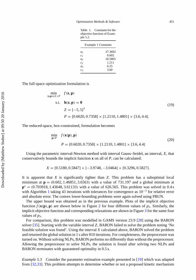
Optimization Methods & Software 451

Table 1. Constants for theobjective function of Exam-ple 5.2.

Example 1 Constants

a1 37.3692c1 0.602a2 18.5805c2 1.211a3 6.25c3 3.60

The full-space optimization formulation is

min(z,p)∈Z×P

f (z, p)

s.t. h(z, p) = 0

Z = [−5, 5]3

P = [0.6020, 0.7358] × [1.2110, 1.4801] × [3.6, 4.4].

(19)

The reduced-space, box-constrained, formulation becomes

minp∈P

f (x(p), p)

P = [0.6020, 0.7358] × [1.2110, 1.4801] × [3.6, 4.4](20)

Using the parametric interval-Newton method with interval Gauss–Seidel, an interval, X, thatconservatively bounds the implicit function x on all of P, can be calculated:

X = [0.5180, 0.5847] × [−3.9748, −3.0464] × [0.3296, 0.5827].

It is apparent that X is significantly tighter than Z . This problem has a suboptimal localminimum at p = (0.602, 1.46851, 3.6563) with a value of 731.197 and a global minimum atp∗ = (0.703918, 1.43648, 3.61133) with a value of 626.565. This problem was solved in 0.4 swith Algorithm 1 taking 43 iterations with tolerances for convergence as 10−3 for relative errorand absolute error. The convex lower-bounding problems were again solved using PBUN.

The upper bound was obtained as in the previous example. Plots of the implicit objectivefunction f (x(p), p) are shown below in Figure 2 for four different values of p3. Similarly, theimplicit objective function and corresponding relaxations are shown in Figure 3 for the same fourvalues of p3.

For comparison, this problem was modelled in GAMS version 23.9 [28] using the BARONsolver [35]. Starting with the variable interval Z , BARON failed to solve the problem noting ‘Nofeasible solution was found’. Using the interval X calculated above, BARON solved the problemand returned the global solution in 1 s after 810 iterations. For completeness, the preprocessor wasturned on. Without solving NLPs, BARON performs no differently than without the preprocessor.Allowing the preprocessor to solve NLPs, the solution is found after solving two NLPs andBARON terminates with guaranteed optimality in 0.5 s.

Example 5.3 Consider the parameter estimation example presented in [19] which was adaptedfrom [32,33]. This problem attempts to determine whether or not a proposed kinetic mechanism

Dow

nloa

ded

by [

Mat

thew

Stu

ber]

at 0

9:50

20

Janu

ary

2016

452 M.D. Stuber et al.

Figure 2. The objective function of Example 5.2 on P1 × P2 at three different p3 values.

sufficiently predicts the behaviour of a reacting system for which experimental data are available.The following kinetic mechanism is proposed:

Z + Yk1−→ A, A + O2

k2f←→k2f /K2

D,

A + O2k3f←→

k3f /K2

B, Bk4−→ M + N ,

2Ak5−→ P,

which is modelled as a system of nonlinear ordinary differential equations (ODEs):

dcA

dt= k1cZcY − cO2(k2f + k3f )cA + k2f

K2cD + k3f

K3cB − k5c2

A,

dcB

dt= k3f cO2 cA −

(k3f

K3+ k4

)cB,

dcD

dt= k2f cAcO2 − k2f

K2cD,

dcY

dt= −k1scY cZ ,

dcZ

dt= −k1cY cZ ,

cA(t = 0) = 0, cB(t = 0) = 0, cD(t = 0) = 0, cY (t = 0) = 0.4, cZ(t = 0) = 140,(21)

Dow

nloa

ded

by [

Mat

thew

Stu

ber]

at 0

9:50

20

Janu

ary

2016

Optimization Methods & Software 453

Figure 3. The objective function of Example 5.2 on P1 × P2 at three different p3 values and corresponding convex andconcave relaxations.

where cj is the concentration (in appropriate units) of species j, T = 273, K2 = 46 exp[6500/T −18], K3 = 2K2, k1 = 53, k1s = k1 × 10−6, k5 = 1.2 × 10−3, and cO2 = 2 × 10−3. The uncer-tain model parameters are p = (k2f , k3f , k4) with k2f ∈ [10, 1200], k3f ∈ [10, 1200], and k4 ∈[0.001, 40]. Each experimental measurement is given in the form of Id = cA + 2

21 cB + 221 cD which

comes from the Beer–Lambert law for relating measured absorbance to concentration with a cor-rection for multiple species [32]. The same data used in [19] is used here and can be downloadedfrom http://yoric.mit.edu/libMC/libmckinexdata.txt.

Using the implicit-Euler discretization scheme, the time domain is discretized into n = 200evenly spaced nodes and the solution of the ODE system (21) can be approximated, with reasonableaccuracy, as the solution of a corresponding nonlinear algebraic system with 5n state variablesand 3 parameters. The method of Mitsos et al. [19] was not applicable to this implicit schemeand so in [19] the method was demonstrated using the explicit-Euler discretization scheme. As anaside, approximating the solution of an ODE system using the explicit-Euler numerical integrationmethod may suffer from numerical instabilities when the problem is stiff (i.e. when the solutionexhibits fast transient behaviour) whereas the implicit technique, albeit more computationallyexpensive per time step, is unconditionally stable and can therefore handle much larger time stepsthan the explicit approach. However, it should be noted that unconditional stability does not implythat the solution is reasonably accurate for large time steps. The ODE (21) is considered to bemoderately stiff and so either approach may work well. For i = 1, . . . , n, the resulting nonlinear

Dow

nloa

ded

by [

Mat

thew

Stu

ber]

at 0

9:50

20

Janu

ary

2016

454 M.D. Stuber et al.

Figure 4. (Left) The sparsity pattern of the system with n = 7 discretization. Each 5 × 5 block is highlighted to showhow the system can be solved in a sequential block-by-block fashion. (Right) An expanded view of three time stepsshowing how information from the previous node is used to solve the 5 × 5 system associated with the current node.

algebraic system is

0 = ci−1A − ci

A + �t

(k1ci

Y ciZ − cO2(k2f + k3f )c

iA + k2f

K2ci

D + k3f

K3ci

B − k5ciA

2)

,

0 = ci−1B − ci

B + �t

(k3f cO2 c

iA −

(k3f

K3+ k4

)ci

B

),

0 = ci−1D − ci

D + �t

(k2f c

iAcO2 − k2f

K2ci

D

),

0 = ci−1Y − ci

Y + �t(−k1sciY ci

Z),

0 = ci−1Z − ci

Z + �t(−k1ciY ci

Z),

(22)

where for n = 200, �t = 0.01. The resulting explicit NLP formulation therefore has 5n + 3variables with

z = (c1A, c1

B, c1D, c1

Y , c1Z , . . . , . . . , . . . , . . . , . . . , c200

A , c200B , c200

D , c200Y , c200

Z ).

By solving the system for the state variables as implicit functions of the parameters, the resultingimplicit NLP formulation has just 3 independent variables. This can be done using two differenttechniques. The first, which is not recommended, is to treat the nonlinear system of equationsas fully coupled and essentially solve for the state variables simultaneously. Thus, in order toconstruct relaxations of implicit functions, using this technique would require relaxing 1000implicit functions simultaneously. The second technique, which is how numerical integration istypically performed, exploits the block structure of the problem.

Taking a look at the sparsity pattern of the system, a portion of which is shown in Figure 4,it is easy to notice that each equation at node i is only dependent on the variables at node i andthe variables at node i − 1. Therefore, if the variables at node i − 1 are known, node i can besolved as a system of five nonlinear equations. Since node 0 is specified by the initial conditions,this technique can be applied sequentially from node 1 to node 200. Again, this is how theimplicit-Euler numerical integration method is applied. Constructing relaxations is then done inan analogous fashion. Relaxations are constructed for each system of 5 equations using the methodof Section 3.4 and subsequently used in the construction of relaxations of each system associated

Dow

nloa

ded

by [

Mat

thew

Stu

ber]

at 0

9:50

20

Janu

ary

2016

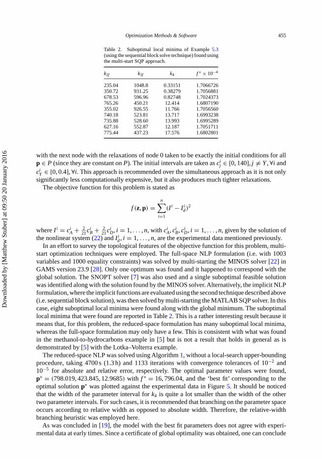
Optimization Methods & Software 455

Table 2. Suboptimal local minima of Example 5.3(using the sequential block solve technique) found usingthe multi-start SQP approach.

k2f k3f k4 f ∗ × 10−4

235.04 1048.8 0.33151 1.7066726350.72 931.25 0.38279 1.7056881678.53 596.96 0.82748 1.7024373765.26 450.21 12.414 1.6807190355.02 926.55 11.766 1.7056560740.18 523.81 13.717 1.6993238735.88 528.60 13.993 1.6995289627.16 552.87 12.187 1.7051711775.44 437.23 17.576 1.6802801

with the next node with the relaxations of node 0 taken to be exactly the initial conditions for allp ∈ P (since they are constant on P). The initial intervals are taken as ci

j ∈ [0, 140], j �= Y , ∀i andci

Y ∈ [0, 0.4], ∀i. This approach is recommended over the simultaneous approach as it is not onlysignificantly less computationally expensive, but it also produces much tighter relaxations.

The objective function for this problem is stated as

f (z, p) =n∑

i=1

(I i − I id)

2

where I i = ciA + 2

21 ciB + 2

21 ciD, i = 1, . . . , n, with ci

A, ciB, ci

D, i = 1, . . . , n, given by the solution ofthe nonlinear system (22) and Ii

d , i = 1, . . . , n, are the experimental data mentioned previously.In an effort to survey the topological features of the objective function for this problem, multi-

start optimization techniques were employed. The full-space NLP formulation (i.e. with 1003variables and 1000 equality constraints) was solved by multi-starting the MINOS solver [22] inGAMS version 23.9 [28]. Only one optimum was found and it happened to correspond with theglobal solution. The SNOPT solver [7] was also used and a single suboptimal feasible solutionwas identified along with the solution found by the MINOS solver. Alternatively, the implicit NLPformulation, where the implicit functions are evaluated using the second technique described above(i.e. sequential block solution), was then solved by multi-starting the MATLAB SQP solver. In thiscase, eight suboptimal local minima were found along with the global minimum. The suboptimallocal minima that were found are reported in Table 2. This is a rather interesting result because itmeans that, for this problem, the reduced-space formulation has many suboptimal local minima,whereas the full-space formulation may only have a few. This is consistent with what was foundin the methanol-to-hydrocarbons example in [5] but is not a result that holds in general as isdemonstrated by [5] with the Lotka–Volterra example.

The reduced-space NLP was solved using Algorithm 1, without a local-search upper-boundingprocedure, taking 4700 s (1.3 h) and 1133 iterations with convergence tolerances of 10−2 and10−5 for absolute and relative error, respectively. The optimal parameter values were found,p∗ = (798.019, 423.845, 12.9685) with f ∗ = 16, 796.04, and the ‘best fit’ corresponding to theoptimal solution p∗ was plotted against the experimental data in Figure 5. It should be noticedthat the width of the parameter interval for k4 is quite a lot smaller than the width of the othertwo parameter intervals. For such cases, it is recommended that branching on the parameter spaceoccurs according to relative width as opposed to absolute width. Therefore, the relative-widthbranching heuristic was employed here.

As was concluded in [19], the model with the best fit parameters does not agree with experi-mental data at early times. Since a certificate of global optimality was obtained, one can conclude

Dow

nloa

ded

by [

Mat

thew

Stu

ber]

at 0

9:50

20

Janu

ary

2016

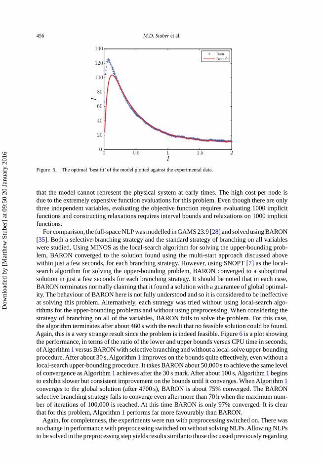
456 M.D. Stuber et al.

Figure 5. The optimal ‘best fit’ of the model plotted against the experimental data.

that the model cannot represent the physical system at early times. The high cost-per-node isdue to the extremely expensive function evaluations for this problem. Even though there are onlythree independent variables, evaluating the objective function requires evaluating 1000 implicitfunctions and constructing relaxations requires interval bounds and relaxations on 1000 implicitfunctions.

For comparison, the full-space NLP was modelled in GAMS 23.9 [28] and solved using BARON[35]. Both a selective-branching strategy and the standard strategy of branching on all variableswere studied. Using MINOS as the local-search algorithm for solving the upper-bounding prob-lem, BARON converged to the solution found using the multi-start approach discussed abovewithin just a few seconds, for each branching strategy. However, using SNOPT [7] as the local-search algorithm for solving the upper-bounding problem, BARON converged to a suboptimalsolution in just a few seconds for each branching strategy. It should be noted that in each case,BARON terminates normally claiming that it found a solution with a guarantee of global optimal-ity. The behaviour of BARON here is not fully understood and so it is considered to be ineffectiveat solving this problem. Alternatively, each strategy was tried without using local-search algo-rithms for the upper-bounding problems and without using preprocessing. When considering thestrategy of branching on all of the variables, BARON fails to solve the problem. For this case,the algorithm terminates after about 460 s with the result that no feasible solution could be found.Again, this is a very strange result since the problem is indeed feasible. Figure 6 is a plot showingthe performance, in terms of the ratio of the lower and upper bounds versus CPU time in seconds,ofAlgorithm 1 versus BARON with selective branching and without a local-solve upper-boundingprocedure. After about 30 s, Algorithm 1 improves on the bounds quite effectively, even without alocal-search upper-bounding procedure. It takes BARON about 50,000 s to achieve the same levelof convergence as Algorithm 1 achieves after the 30 s mark. After about 100 s, Algorithm 1 beginsto exhibit slower but consistent improvement on the bounds until it converges. When Algorithm 1converges to the global solution (after 4700 s), BARON is about 75% converged. The BARONselective branching strategy fails to converge even after more than 70 h when the maximum num-ber of iterations of 100,000 is reached. At this time BARON is only 97% converged. It is clearthat for this problem, Algorithm 1 performs far more favourably than BARON.

Again, for completeness, the experiments were run with preprocessing switched on. There wasno change in performance with preprocessing switched on without solving NLPs. Allowing NLPsto be solved in the preprocessing step yields results similar to those discussed previously regarding

Dow

nloa

ded

by [

Mat

thew

Stu

ber]

at 0

9:50

20

Janu

ary

2016

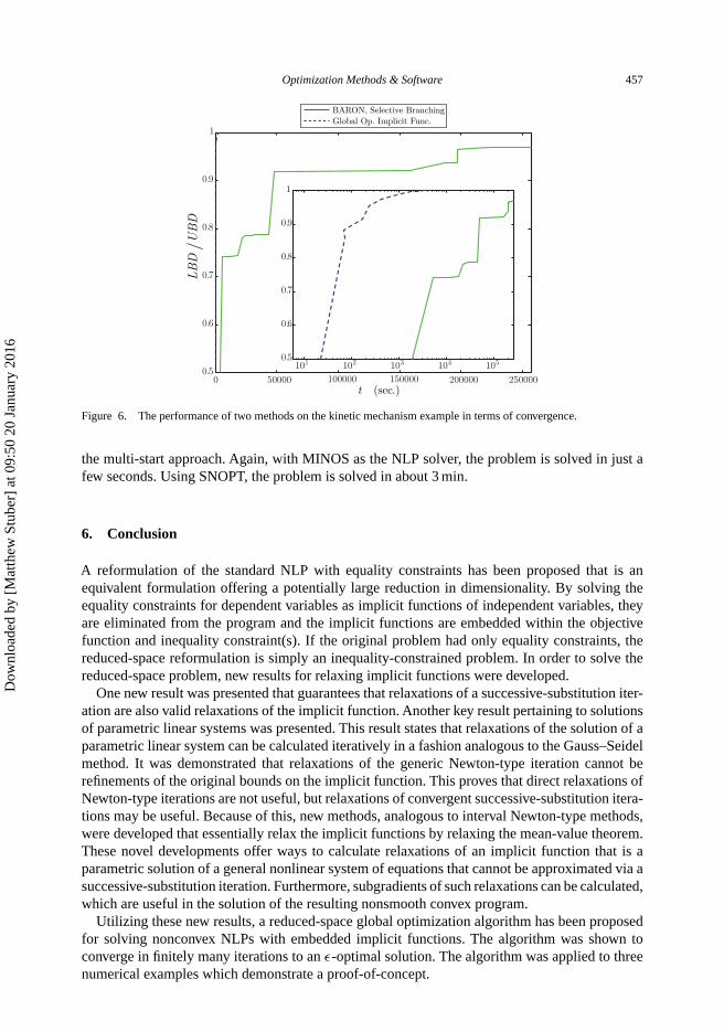
Optimization Methods & Software 457

Figure 6. The performance of two methods on the kinetic mechanism example in terms of convergence.

the multi-start approach. Again, with MINOS as the NLP solver, the problem is solved in just afew seconds. Using SNOPT, the problem is solved in about 3 min.

6. Conclusion

A reformulation of the standard NLP with equality constraints has been proposed that is anequivalent formulation offering a potentially large reduction in dimensionality. By solving theequality constraints for dependent variables as implicit functions of independent variables, theyare eliminated from the program and the implicit functions are embedded within the objectivefunction and inequality constraint(s). If the original problem had only equality constraints, thereduced-space reformulation is simply an inequality-constrained problem. In order to solve thereduced-space problem, new results for relaxing implicit functions were developed.

One new result was presented that guarantees that relaxations of a successive-substitution iter-ation are also valid relaxations of the implicit function. Another key result pertaining to solutionsof parametric linear systems was presented. This result states that relaxations of the solution of aparametric linear system can be calculated iteratively in a fashion analogous to the Gauss–Seidelmethod. It was demonstrated that relaxations of the generic Newton-type iteration cannot berefinements of the original bounds on the implicit function. This proves that direct relaxations ofNewton-type iterations are not useful, but relaxations of convergent successive-substitution itera-tions may be useful. Because of this, new methods, analogous to interval Newton-type methods,were developed that essentially relax the implicit functions by relaxing the mean-value theorem.These novel developments offer ways to calculate relaxations of an implicit function that is aparametric solution of a general nonlinear system of equations that cannot be approximated via asuccessive-substitution iteration. Furthermore, subgradients of such relaxations can be calculated,which are useful in the solution of the resulting nonsmooth convex program.

Utilizing these new results, a reduced-space global optimization algorithm has been proposedfor solving nonconvex NLPs with embedded implicit functions. The algorithm was shown toconverge in finitely many iterations to an ε-optimal solution. The algorithm was applied to threenumerical examples which demonstrate a proof-of-concept.

Dow

nloa

ded

by [

Mat

thew

Stu

ber]

at 0

9:50

20

Janu

ary

2016

458 M.D. Stuber et al.

Acknowledgements

The authors would like to acknowledge the Chevron University Partnership Program for supporting this work through theMIT Energy Initiative (MITEI/UPP). The authors would also like to give a special acknowledgement to Harry Watson forhis contribution to the kinetic model example (Example 5.3).

References

[1] C.S.Adjiman and C.A. Floudas, Rigorous convex underestimators for general twice-differentiable problems, J. GlobalOptim. 9 (1996), pp. 23–40.

[2] C. Bendtsen and O. Stauning, FADBAD, a flexible C++ package for automatic differentiation, Tech. Rep. 1996-x5-94,Technical University of Denmark, Lyngby, Denmark, 1996.

[3] B. Chachuat, MC++: A versatile library for McCormick relaxations and Taylor models. Available athttp://www3.imperial.ac.uk/people/b.chachuat/research.

[4] T.G. Epperly and E.N. Pistikopoulos, A reduced space branch and bound algorithm for global optimization, J. GlobalOptim. 11 (1997), pp. 287–311.

[5] W.R. Esposito and C.A. Floudas, Global optimization for the parameter estimation of differential-algebraic systems,Ind. Eng. Chem. Res. 39 (2000), pp. 1291–1310.

[6] J.E. Falk and R.M. Soland, An algorithm for separable nonconvex programming problems, Manag. Sci. 15 (1969),pp. 550–569.

[7] P.E. Gill, W. Murray, and M.A. Saunders, SNOPT: An SQP algorithm for large-scale constrained optimization,SIAM Rev. 47 (2005), pp. 99–131.

[8] A. Griewank and A. Walther, Evaluating Derivatives: Principles and Techniques of Automatic Differentiation, 2nded., SIAM, Philadelphia, PA, 2008.

[9] E.R. Hansen and R.I. Greenberg, Interval Newton methods, Appl. Math. Comput. 12 (1983), pp. 89–98.[10] E. Hansen and G.W. Walster, Global Optimization Using Interval Analysis, 2nd ed., Marcel Dekker, NewYork, 2004.[11] R. Horst, A general class of branch-and-bound methods in global optimization with some new approaches for

concave minimization, J. Optim. Theory Appl. 51 (1986), pp. 271–291.[12] R. Horst, Deterministic global optimization with partition sets whose feasibility is not known: Application to concave

minimization, reverse convex constraints, DC-programming, and Lipschitzian optimization, J. Optim. Theory Appl.58 (1988), pp. 11–37.

[13] R. Horst and N.V. Thoai, Conical algorithm for the global minimization of linearly constrained decomposableconcave minimization problems, J. Optim. Theory Appl. 74 (1992), pp. 469–486.

[14] R. Horst and N.V. Thoai, Constraint decomposition algorithms in global optimization, J. Global Optim. 5 (1994),pp. 333–348.

[15] R. Horst and H. Tuy, Global Optimization: Deterministic Approaches, 3rd ed., Springer, Berlin, 1996.[16] R.B. Kearfott, Preconditioners for the interval Gauss-Seidel method, SIAM J. Numer. Anal. 27 (1990), pp. 804–822.[17] L. Luksan and J. Vlcek, Algorithms for non-differentiable optimization, ACM Trans. Math. Soft. 27 (2001),

pp. 193–213.[18] G.P. McCormick, Computability of global solutions to factorable nonconvex programs: Part I—convex underesti-

mating problems, Math. Program 10 (1976), pp. 147–175.[19] A. Mitsos, B. Chachuat, and P.I. Barton, McCormick-based relaxations of algorithms, SIAM J. Optim. 20 (2009),

pp. 573–601.[20] R.E. Moore, Methods and Applications of Interval Analysis, SIAM, Philadelphia, PA, 1979.[21] J.R. Munkres, Analysis on Manifolds, Westview Press, Boulder, CO, 1991.[22] B.A. Murtagh and M.A. Saunders, MINOS 5.5 user’s guide, Tech. Rep., Stanford University, Stanford, CA, 1983.[23] L.D. Muu and W. Oettli, Combined branch-and-bound and cutting plane methods for solving a class of nonlinear

programming problems, J. Global Optim. 3 (1993), pp. 377–391.[24] A. Neumaier, Interval Methods for Systems of Equations, Cambridge University Press, Cambridge, 1990.[25] J.M. Ortega and W.C. Rheinboldt, Iterative Solution of Nonlinear Equations in Several Variables, Academic Press,

Inc., Boston, MA, 1970.[26] A.T. Phillips and J.B. Rosen, A parallel algorithm for constrained concave quadratic global optimization, Math.

Program. 42 (1988), pp. 421–448.[27] E.D. Popova, On the solution of parametrised linear systems, in Scientific Computing, Validated Numerics, Interval

Methods, K. Walter von Gudenberg and J. Wolff, eds., KluwerAcademic Publishers, Boston, MA, 2001, pp. 127–138.[28] R.E. Rosenthal, GAMS—A User’s Manual, Washington, DC, 2012.[29] W. Rudin, Principles of Mathematical Analysis, 3rd ed., McGraw-Hill, New York, 1976.[30] H.S. Ryoo and N.V. Sahinidis, A branch-and-reduce approach to global optimization, J. Global Optim. 8 (1996),

pp. 107–138.[31] J.K. Scott, M.D. Stuber, and P.I. Barton, Generalized McCormick relaxations, J. Global Optim. 51 (2011),

pp. 569–606.[32] A.B. Singer, Global dynamic optimization, Ph.D. thesis, Massachusetts Institute of Technology, 2004.[33] A.B. Singer, J.W. Taylor, P.I. Barton, and W.H. Green, Global dynamic optimization for parameter estimation in

chemical kinetics, J. Phys. Chem. A 110 (2006), pp. 971–976.

Dow

nloa

ded

by [

Mat

thew

Stu

ber]

at 0

9:50

20

Janu

ary

2016

Optimization Methods & Software 459

[34] M.D. Stuber, Evaluation of process systems operating envelopes, Ph.D. thesis, Massachusetts Institute of Technology,2013.

[35] M. Tawarmalani and N.V. Sahinidis, A polyhedral branch-and-cut approach to global optimization, Math. Program.103(2) (2005), pp. 225–249.

Appendix 1. Parameterized generalized bisection

Calculating an interval X such that existence and uniqueness of an enclosed implicit function x(p), ∀p ∈ P is guaranteed,a prerequisite for applying Algorithm 1, is still an open research topic. One such method, discussed in length in [34] is theparameterized generalized bisection procedure. This implementation of the generalized bisection procedure accounts forthe parameter dimension by eliminating the situation referred to as a partial enclosure, whereby x(p) ∈ X only for somevalues of p ∈ P. Such a partial enclosure situation is likely if the X dimension were to be blindly bisected as in the standardgeneralized bisection procedure. Furthermore, there may not exist a cut in the X dimension such that the partial enclosuresituation can be avoided without also considering partitioning P. Such is the case when multiple solution branches arelocated near one another. Therefore, both the X and P dimensions must be systematically partitioned. Figure A1 illustratesthis idea.

The overall objective then is to produce intervals Xi × Pj , i = 1, . . . , nj , j = 1, . . . m such that the Pj are as large aspossible. Furthermore, ∪jPj = P and ∪j ∪i=1,...,nj Xi × Pj covers the entire solution set on P with a unique continuoussolution branch in each Xi × Pj . The algorithmic framework is given below.

Algorithm 2

(1) Initialization(a) Pick initial box (X0, P0), initialize solution set � and stack S = {(X0, P0)}. Set iteration count l := 0.

(2) Termination(a) Stack empty? (S = ∅?)

(i) Yes. Algorithm terminates.(ii) No. Pop and delete a box (Z , P) from stack S , set l := l + 1.

(b) If 0 ∈ H(Z , P), go to 4. Else, go to 2 ((Z , P) has been fathomed).(3) Interval Refinement

(a) Apply parametric interval-Newton-type iteration with extended division starting at Z0 := Z.(i) If any iteration k yields two disjoint intervals, labelled ZL and ZR, by extended division, place (ZL , P) and

(ZR, P) on S . Go to 2.(ii) At every iteration k, apply the standard interval inclusion test.

(a). If the interval-Newton-type operator yields an empty interval, go to 2, (Z , P) has been fathomed.(iii) If the iteration converges and the inclusion test has never been passed, go to 4. Else, place (Zk , P) in solution

set �, go to 2.(4) Improved Existence and Uniqueness Test

(a) Apply a sharper existence and uniqueness test.(i) If test is passed, place (Zk , P) on solution set �, go to 2. Else, continue.

(ii) If test is failed but partial enclosure possibility is excluded, go to 5. Else, go to 6.(5) Partition X Direction

(a) Partition Z using some strategy to avoid creating partial enclosures and add the resulting boxes to the stack S .

(a) (b)

Figure A1. (a)A box X × P in which there does not exist a position to cut X (dashed lines) such that no partial enclosuresare produced. (b) After partitioning P, there exist positions to cut X avoiding partial enclosures.

Dow

nloa

ded

by [

Mat

thew

Stu

ber]

at 0

9:50

20

Janu

ary

2016

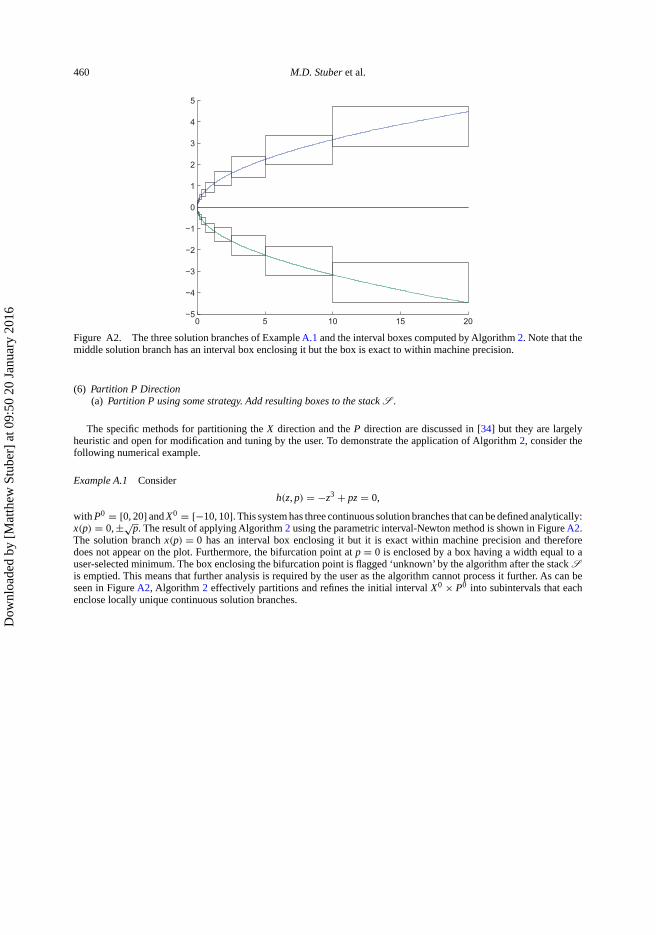
460 M.D. Stuber et al.

Figure A2. The three solution branches of Example A.1 and the interval boxes computed by Algorithm 2. Note that themiddle solution branch has an interval box enclosing it but the box is exact to within machine precision.

(6) Partition P Direction(a) Partition P using some strategy. Add resulting boxes to the stack S .

The specific methods for partitioning the X direction and the P direction are discussed in [34] but they are largelyheuristic and open for modification and tuning by the user. To demonstrate the application of Algorithm 2, consider thefollowing numerical example.

Example A.1 Consider

h(z, p) = −z3 + pz = 0,

with P0 = [0, 20] and X0 = [−10, 10]. This system has three continuous solution branches that can be defined analytically:x(p) = 0, ±√

p. The result of applying Algorithm 2 using the parametric interval-Newton method is shown in Figure A2.The solution branch x(p) = 0 has an interval box enclosing it but it is exact within machine precision and thereforedoes not appear on the plot. Furthermore, the bifurcation point at p = 0 is enclosed by a box having a width equal to auser-selected minimum. The box enclosing the bifurcation point is flagged ‘unknown’ by the algorithm after the stack Sis emptied. This means that further analysis is required by the user as the algorithm cannot process it further. As can beseen in Figure A2, Algorithm 2 effectively partitions and refines the initial interval X0 × P0 into subintervals that eachenclose locally unique continuous solution branches.

Dow

nloa

ded

by [

Mat

thew

Stu

ber]

at 0

9:50

20

Janu

ary

2016