convex analysis of submodular set functions for machine learning
TRANSCRIPT

Convex Analysis for Minimizing and Learning Submodular SetFunctions
Thesis by
Peter Stobbe
In Partial Fulfillment of the Requirements
for the Degree of
Doctor of Philosophy
California Institute of Technology
Pasadena, California
2013
(Defended May 16, 2013)

ii
c© 2013
Peter Stobbe
All Rights Reserved

iii
To Aura

iv
Abstract
The connections between convexity and submodularity are explored, for purposes of mini-
mizing and learning submodular set functions.
First, we develop a novel method for minimizing a particular class of submodular functions,
which can be expressed as a sum of concave functions composed with modular functions.
The basic algorithm uses an accelerated first order method applied to a smoothed version of
its convex extension. The smoothing algorithm is particularly novel as it allows us to treat
general concave potentials without needing to construct a piecewise linear approximation as
with graph-based techniques.
Second, we derive the general conditions under which it is possible to find a minimizer of
a submodular function via a convex problem. This provides a framework for developing sub-
modular minimization algorithms. The framework is then used to develop several algorithms
that can be run in a distributed fashion. This is particularly useful for applications where the
submodular objective function consists of a sum of many terms, each term dependent on a
small part of a large data set.
Lastly, we approach the problem of learning set functions from an unorthodox perspective—
sparse reconstruction. We demonstrate an explicit connection between the problem of
learning set functions from random evaluations and that of sparse signals. Based on the
observation that the Fourier transform for set functions satisfies exactly the conditions needed
for sparse reconstruction algorithms to work, we examine some different function classes
under which uniform reconstruction is possible.

v
Contents
List of Figures vii
List of Algorithms viii
1 Introduction 1
1.1 Main Contributions . . . . . . . . . . . . . . . . . . . . . . . . . . . . . . . . . . . . 3
1.2 Outline of Thesis . . . . . . . . . . . . . . . . . . . . . . . . . . . . . . . . . . . . . 4
2 Background of Convex Analysis 5
2.1 Basic Concepts . . . . . . . . . . . . . . . . . . . . . . . . . . . . . . . . . . . . . . . 5
2.2 Proximal Operators . . . . . . . . . . . . . . . . . . . . . . . . . . . . . . . . . . . . 8
3 Set Functions and Submodularity 12
3.1 Overview . . . . . . . . . . . . . . . . . . . . . . . . . . . . . . . . . . . . . . . . . . 12
3.2 General Set Functions . . . . . . . . . . . . . . . . . . . . . . . . . . . . . . . . . . 12
3.2.1 Set Function Derivatives . . . . . . . . . . . . . . . . . . . . . . . . . . . . 14
3.2.2 Monotone and Low Order Functions . . . . . . . . . . . . . . . . . . . . . 16
3.2.3 Fourier Analysis of Set Functions . . . . . . . . . . . . . . . . . . . . . . . 18
3.2.4 Tensor Product Bases of Set Functions . . . . . . . . . . . . . . . . . . . . 20
3.3 Properties of Submodular Set Functions . . . . . . . . . . . . . . . . . . . . . . . 22
3.3.1 Convex Analysis of Submodularity . . . . . . . . . . . . . . . . . . . . . . 23
3.3.2 Lovász Extension . . . . . . . . . . . . . . . . . . . . . . . . . . . . . . . . . 27
3.3.3 Examples of Base Polytopes . . . . . . . . . . . . . . . . . . . . . . . . . . 29
3.4 Submodular Minimization . . . . . . . . . . . . . . . . . . . . . . . . . . . . . . . . 30
3.4.1 Ellipsoid Method and Polynomial Time Algorithms . . . . . . . . . . . . 31
3.4.2 Fujishige’s Minimal Norm Algorithm . . . . . . . . . . . . . . . . . . . . . 33

vi
3.4.3 Special Cases . . . . . . . . . . . . . . . . . . . . . . . . . . . . . . . . . . . 33
4 Smoothed Gradient Methods for Decomposable Functions 35
4.1 Introduction . . . . . . . . . . . . . . . . . . . . . . . . . . . . . . . . . . . . . . . . 35
4.2 Background on Submodular Function Minimization . . . . . . . . . . . . . . . . 35
4.3 The Decomposable Submodular Minimization Problem . . . . . . . . . . . . . . 38
4.4 Classification of Submodular Functions . . . . . . . . . . . . . . . . . . . . . . . . 40
4.4.1 Submodularity of Decomposable Functions . . . . . . . . . . . . . . . . . 40
4.4.2 Set Cover Functions as Threshold Potentials . . . . . . . . . . . . . . . . 41
4.4.3 Reformulation of a Class of Functions . . . . . . . . . . . . . . . . . . . . 42
4.4.4 Strict Generality of Threshold Potentials . . . . . . . . . . . . . . . . . . 43
4.5 The SLG Algorithm for Threshold Potentials . . . . . . . . . . . . . . . . . . . . . 44
4.5.1 The Smoothed Extension of a Threshold Potential . . . . . . . . . . . . 44
4.5.2 The SLG Algorithm for Minimizing Sums of Threshold Potentials . . . 46
4.5.3 Early Stopping based on Discrete Certificates of Optimality . . . . . . . 48
4.6 Extension to General Concave Potentials . . . . . . . . . . . . . . . . . . . . . . . 50
4.6.1 Formula Derivation . . . . . . . . . . . . . . . . . . . . . . . . . . . . . . . 51
4.7 Experiments . . . . . . . . . . . . . . . . . . . . . . . . . . . . . . . . . . . . . . . . 53
4.8 Conclusion . . . . . . . . . . . . . . . . . . . . . . . . . . . . . . . . . . . . . . . . . 56
5 Distributed Submodular Minimization 57
5.1 Introduction . . . . . . . . . . . . . . . . . . . . . . . . . . . . . . . . . . . . . . . . 57
5.2 Submodular Minimization with General Barrier Functions . . . . . . . . . . . . 58
5.3 Consensus Algorithms for Submodular Minimization . . . . . . . . . . . . . . . 63
5.3.1 Notation . . . . . . . . . . . . . . . . . . . . . . . . . . . . . . . . . . . . . . 63
5.3.2 Outline of Algorithms . . . . . . . . . . . . . . . . . . . . . . . . . . . . . . 64
5.4 Fast Proximal Threshold Potentials . . . . . . . . . . . . . . . . . . . . . . . . . . 66
5.4.1 General Plane Intersection Projection . . . . . . . . . . . . . . . . . . . . 66
5.4.2 Box-Plane Projection Algorithms . . . . . . . . . . . . . . . . . . . . . . . 67
5.5 Experiments . . . . . . . . . . . . . . . . . . . . . . . . . . . . . . . . . . . . . . . . 69
6 Learning Fourier Sparse Set Functions 75
6.1 Introduction . . . . . . . . . . . . . . . . . . . . . . . . . . . . . . . . . . . . . . . . 75

vii
6.2 Background . . . . . . . . . . . . . . . . . . . . . . . . . . . . . . . . . . . . . . . . . 77
6.2.1 The Fourier transform on set functions. . . . . . . . . . . . . . . . . . . . 77
6.3 Conditions for Recovery . . . . . . . . . . . . . . . . . . . . . . . . . . . . . . . . . 78
6.4 Classes of Set Functions . . . . . . . . . . . . . . . . . . . . . . . . . . . . . . . . . 80
6.4.1 Symmetric functions. . . . . . . . . . . . . . . . . . . . . . . . . . . . . . . 81
6.4.2 Low order functions. . . . . . . . . . . . . . . . . . . . . . . . . . . . . . . 81
6.4.3 Submodular functions. . . . . . . . . . . . . . . . . . . . . . . . . . . . . . 82
6.5 Reconstruction Algorithms . . . . . . . . . . . . . . . . . . . . . . . . . . . . . . . 85
6.5.1 Exploiting structure in the Fourier domain. . . . . . . . . . . . . . . . . . 86
6.6 Applications and Experiments . . . . . . . . . . . . . . . . . . . . . . . . . . . . . 86
6.6.1 Sketching graph evolution . . . . . . . . . . . . . . . . . . . . . . . . . . . 86
6.6.2 Approximate submodular optimization . . . . . . . . . . . . . . . . . . . 88
6.6.3 Synthetic Submodular Recovery . . . . . . . . . . . . . . . . . . . . . . . 89
6.7 Related Work . . . . . . . . . . . . . . . . . . . . . . . . . . . . . . . . . . . . . . . . 90
6.8 Conclusion . . . . . . . . . . . . . . . . . . . . . . . . . . . . . . . . . . . . . . . . . 92
7 Conclusion 94
A Matroid Theory 96
Bibliography 99
viii
List of Figures
4.1 Example Regions and Comparision of Submodular Minimization Running Times 54
4.2 Segmentation Experimental Results . . . . . . . . . . . . . . . . . . . . . . . . . . 55
5.1 Synthetic Problem . . . . . . . . . . . . . . . . . . . . . . . . . . . . . . . . . . . . . 71
5.2 Parallelization Speedup . . . . . . . . . . . . . . . . . . . . . . . . . . . . . . . . . . 72
5.3 FISTA convergence . . . . . . . . . . . . . . . . . . . . . . . . . . . . . . . . . . . . . 73
5.4 Barzilai–Borwein Convergence . . . . . . . . . . . . . . . . . . . . . . . . . . . . . . 74
6.1 Graph Reconstruction and Approximate Optimization Results . . . . . . . . . . . 87
6.2 Empirical Study of Submodular Constraints . . . . . . . . . . . . . . . . . . . . . . 91

ix
List of Algorithms
4.1 SLG: Smoothed Lovász Gradient . . . . . . . . . . . . . . . . . . . . . . . . . . . . . 48
4.2 Set Generation by Rounding the Continuous Solution . . . . . . . . . . . . . . . 48
4.3 Set Optimality Check . . . . . . . . . . . . . . . . . . . . . . . . . . . . . . . . . . . . 50
4.4 Gradient for General Concave Functions . . . . . . . . . . . . . . . . . . . . . . . . 53
5.1 Projection onto a Box Intersecting a Plane . . . . . . . . . . . . . . . . . . . . . . . 68
5.2 Piecewise Linear Monotonic Root: Sorted Version . . . . . . . . . . . . . . . . . . 69
5.3 Piecewise Linear Monotonic Root: Unsorted Version . . . . . . . . . . . . . . . . 70

1
Chapter 1
Introduction
There is no doubt that convex optimization has proven to be an invaluable tool throughout all
of the applied sciences and engineering. Consider though: the formal definition of convexity
is a completely abstract concept, yet somehow has proven to be key in the development
of numerical algorithms for countless real-world applications. Given the tremendous track
record of such a powerful abstract idea, the mandate of the applied mathematics community
must be then to attempt to answer the question: “Can convexity be generalized? Can we
discover similar abstract concepts that hold the key for solving new, important problems?” And
while one search direction of this quest is to look into the realm of continuous functions for
quasiconvex or invex functions as generalizations, the other is to look for discrete analogues
of convexity. Indeed, many different such discrete generalizations have been discovered
[Mur03], yet none of them could accurately be described as a perfect mirror image of
convexity. But we would claim that there is one such concept from discrete optimization that
in recent years has proven to be the most similar to convexity, not only in terms of its salient
abstract features, but also its empirical problem solving utility: submodularity.
Submodularity is a property of set functions—meaning functions of some subset of a
finite set of objects. It has numerous equivalent definitions, but perhaps the easiest to parse
is the following inequality. It says that the change in value of the set function when adding a
particular element must be smaller when adding it to a larger1 set:
f (A∪ e)− f (A)≥ f (B ∪ e)− f (B), for all elements e and sets A, B such that e /∈ B ⊇ A.
One amazing property of submodularity is that there are powerful algorithms for both maxi-
1By “larger” we mean a superset, not just any set of greater cardinality!
2
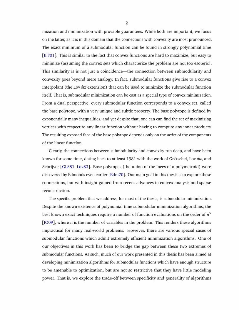
mization and minimization with provable guarantees. While both are important, we focus
on the latter, as it is in this domain that the connections with convexity are most pronounced.
The exact minimum of a submodular function can be found in strongly polynomial time
[IFF01]. This is similar to the fact that convex functions are hard to maximize, but easy to
minimize (assuming the convex sets which characterize the problem are not too esoteric).
This similarity is is not just a coincidence—the connection between submodularity and
convexity goes beyond mere analogy. In fact, submodular functions give rise to a convex
interpolant (the Lovász extension) that can be used to minimize the submodular function
itself. That is, submodular minimization can be cast as a special type of convex minimization.
From a dual perspective, every submodular function corresponds to a convex set, called
the base polytope, with a very unique and subtle property. The base polytope is defined by
exponentially many inequalities, and yet despite that, one can can find the set of maximizing
vertices with respect to any linear function without having to compute any inner products.
The resulting exposed face of the base polytope depends only on the order of the components
of the linear function.
Clearly, the connections between submodularity and convexity run deep, and have been
known for some time, dating back to at least 1981 with the work of Grötschel, Lovász, and
Schrijver [GLS81, Lov83]. Base polytopes (the union of the faces of a polymatroid) were
discovered by Edmonds even earlier [Edm70]. Our main goal in this thesis is to explore these
connections, but with insight gained from recent advances in convex analysis and sparse
reconstruction.
The specific problem that we address, for most of the thesis, is submodular minimization.
Despite the known existence of polynomial-time submodular minimization algorithms, the
best known exact techniques require a number of function evaluations on the order of n5
[IO09], where n is the number of variables in the problem. This renders these algorithms
impractical for many real-world problems. However, there are various special cases of
submodular functions which admit extremely efficient minimization algorithms. One of
our objectives in this work has been to bridge the gap between these two extremes of
submodular functions. As such, much of our work presented in this thesis has been aimed at
developing minimization algorithms for submodular functions which have enough structure
to be amenable to optimization, but are not so restrictive that they have little modeling
power. That is, we explore the trade-off between specificity and generality of algorithms

3
and submodular function classes, not unlike the trade-off of generalization in statistics and
learning. So in this way, the last major part of the thesis is related to what precedes it. Therein
we examine a learning problem, that of set functions. We consider submodular functions in
particular as a class of objects to learn, but what sets this work apart from classical research
on learning set functions is that we use the tools of convex analysis and sparse recovery.
1.1 Main Contributions
In Chapter 4, we develop a novel method for minimizing a particular class of submodular
functions, which can be expressed as a sum of concave functions composed with modular
functions. The basic algorithm uses an accelerated first order method applied to a smoothed
version of the Lovász extension. The smoothing algorithm is particularly novel as it allows us
to treat general concave potentials without needing to construct a piecewise linear approxi-
mation as with graph-based techniques. This is a fully expanded version of work presented
previously [SK10], which did not originally contain the fast method of smoothing.
In Chapter 5, our main technical contribution is elucidating the conditions under which
it is possible to find a minimizer of a submodular function via a convex problem. In general
one minimizes the Lovász extension together with a separable barrier function, and our
Theorem 5.4 gives the weakest conditions yet presented in the literature to guarantee that the
convex problem gives a minimizer of the submodular problem; we demonstrate why these
conditions are necessary, given some mild assumptions. This provides a general framework
for developing submodular minimization algorithms. The framework is then used to develop
several algorithms that can be run in a distributed fashion. This is particularly useful for
applications where the submodular objective function consists of a sum of many terms, each
term dependent on a small part of a large data set.
In Chapter 6 we approach the problem of learning set functions from an unorthodox
perspective—sparse reconstruction. We demonstrate an explicit connection between the
problem of learning set functions from random evaluations and that of sparse signals. Based
on the observation that the Fourier transform for set functions satisfies exactly the conditions
needed for sparse reconstruction algorithms to work, we examine some different function
classes under which uniform reconstruction is possible. In particular, given the values of the
cut function of a graph, we show the graph can be reconstructed. Furthermore, we show

4
how the assumption of submodularity can be encoded as a constraint of a third order set
function and its utility in the reconstruction of a set function.
1.2 Outline of Thesis
• In Chapter 2 we review some concepts from convex analysis and introduce the notation
relevant to convex functions and sets.
• Chapter 3 is dedicated to the background material on submodular set functions. Sec-
tion 3.2 is devoted to the theory of general set functions, whereas in Section 3.3, we
review properties of submodular set functions, deriving several of the main relations to
convexity. In Section 3.4 we discuss submodular minimization.
• In Chapter 4 we describe our Smoothed Lovász Gradient algorithm for the minimization
of decomposable submodular functions. Section 4.4 is dedicated to the classification
and representation of decomposable functions. This was originally presented in [SK10].
• In Chapter 5, we develop consensus algorithms for distributed submodular minimiza-
tion. In Section 5.2, we detail the relationship between convex optimization problems
and the minimizers of a submodular function.
• In Chapter 6, we apply the tools of convex analysis and sparse approximation to the
problem of learning set functions. This was originally presented in [SK12].

5
Chapter 2
Background of Convex Analysis
2.1 Basic Concepts
Throughout this thesis, we will use the convention of convex analysis [Roc70, HUL93, AT03]
that functions are defined everywhere in Rn, but functions can equal +∞. When we refer to
the domain of a function, we mean the set of points where it is finite valued:
dom( f ) := x ∈ Rn | f (x)< +∞
We define the indicator function of a set to be the function that has that set as its domain,
and equals zero there:
δC(x) :=
0 x ∈ C
+∞ x /∈ C(2.1.1)
This means that there is no loss of generality in treating constrained optimization problems as
unconstrained and vice-versa. When we discuss solving minx∈C f (x), where C is some subset
of Rn, it is equivalent to solving the unconstrained problem minx f (x) +δC(x). (Clearly we
can treat an unconstrained problem as a constrained one with empty constraints.) Convex
sets are those which contain every line segment connecting any pair of points in the set.
The convex hull of a set is defined as the intersection of all convex sets containing it:
conv S :=⋂
C⊆S,C convex
C .
We can define convex functions in terms of convex sets. The epigraph of a func-
tion f on Rn is the set of points in Rn+1 that lie above its graph epi f = (x, t) ∈ Rn+1 |
x ∈ dom f , f (x)≤ t . Convex functions are defined as those with a convex epigraph. Con-

6
vex functions are not necessarily differentiable, but instead have subgradients. For convex
f , we define the subdifferential to be the set valued map ∂ f : Rn→ 2Rn
which is the set of
subgradients: linear functionals which bound the function from below.
∂ f (x) := λ ∈ Rn | f (y)≥ f (x) + ⟨y− x,λ⟩ for all y ∈ Rn
Since it is an intersection of half-spaces, the subdifferential is always closed and convex, but
it might be empty, even if the function is convex and finite-valued at that point. At any point
where a convex function is differentiable, the gradient at that point is the unique subgradient:
∂ f (x) = ∇ f (x). Subdifferentials are linear and positive homogenous, where addition is in
the sense of a Minkowski sum:
∂( f1 +α f2) = ∂ f1 +α∂ f2, α≥ 0
A key tool in analyzing the dual of a convex program is the convex conjugate, also known as
the Legendre-Fenchel transform of a function. It is defined as:
f ∗(λ) := supx∈Rn⟨x,λ⟩ − f (x)
This is always convex even if f is not. It is immediate from the definition that:
f (x) + f ∗(λ)≥ ⟨x,λ⟩ for all x,λ ∈ Rn (2.1.2)
Furthermore, note that if λ is a subgradient of f at x, then ⟨y,λ⟩ − f (y)≥ ⟨x,λ⟩ − f (x) for
all y ∈ Rn. So Equation 2.1.2 holds with equality if and only if λ ∈ ∂ f (x).
We denote the set of convex, proper, lower semi-continuous functions as Conv. These
functions obey the useful property that they are equal to their biconjugate.
f ∈ Conv⇔ f ∗∗ = f (2.1.3)
So, for f ∈ Conv, we can make a stronger statement about when Equation 2.1.2 holds with
equality:
f (x) + f ∗(λ) = ⟨x,λ⟩ ⇔ x ∈ ∂ f ∗(λ) ⇔ λ ∈ ∂ f (x)
7
One interpretation of Equation 2.1.3 is that all f ∈ Conv admit the following sort of self-
description:
f (x) = supy,λ
f (y) + ⟨x− y,λ⟩
s.t. λ ∈ ∂ f (y)
In Section 3.3, we show that submodular functions enjoy an analogous property.
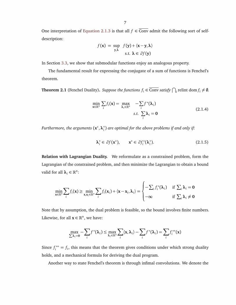
The fundamental result for expressing the conjugate of a sum of functions is Fenchel’s
theorem.
Theorem 2.1 (Fenchel Duality). Suppose the functions fi ∈ Conv satisfy⋂
i relint dom fi 6= ;.
minx∈Rn
∑
ifi(x) = max
λi∈Rn−∑
if ∗(λi)
s.t.∑
iλi = 0
(2.1.4)
Furthermore, the arguments (x∗,λ∗i ) are optimal for the above problems if and only if:
λ∗i ∈ ∂ f (x∗), x∗ ∈ ∂ f ∗i (λ∗i ). (2.1.5)
Relation with Lagrangian Duality. We reformulate as a constrained problem, form the
Lagrangian of the constrained problem, and then minimize the Lagrangian to obtain a bound
valid for all λi ∈ Rn:
minx∈Rn
∑
i
fi(x)≥ minx,xi∈Rn
∑
i
fi(xi) + ⟨x− xi,λi⟩=
−∑
i f ∗i (λi) if∑
i λi = 0
−∞ if∑
i λi 6= 0
Note that by assumption, the dual problem is feasible, so the bound involves finite numbers.
Likewise, for all x ∈ Rn, we have:
max∑
λi=0−∑
i
f ∗(λi)≤ maxλi∈Rn
∑
i
⟨x,λi⟩ −∑
i
f ∗(λi) =∑
i
f ∗∗i (x)
Since f ∗∗i = fi, this means that the theorem gives conditions under which strong duality
holds, and a mechanical formula for deriving the dual program.
Another way to state Fenchel’s theorem is through infimal convolutions. We denote the

8
infimal convolution of functions with the symbol and define it by the following formula:
f g(x) := infy∈Rn
f (x− y) + g(y)
If f and g satisfy conditions sufficient for Fenchel’s duality theorem to hold, then infimal
convolution is essentially the operation which is dual to addition under the Legendre-Fenchel
transform: ( f g)∗ = f ∗ + g∗ and ( f + g)∗ = f ∗ g∗.
2.2 Proximal Operators
A key step in many convex minimization algorithms is solving for the infimal convolution
of an objective function with a quadratic function at the current iterate. For any function
f ∈ Conv, we define its proximal operator or ‘prox’ as:
prox f (x) := arg miny∈Rn
f (y) +1
2‖x− y‖2 (2.2.1)
For a thorough explanation of the proximal operator, see [CP11]. We review a few important
ideas and identities.
By strong convexity of the quadratic term, the minimum is a unique point so the prox
is well-defined. (In its most general form, one can use any Bregman distance [Brè67] in
place of the quadratic, but the present definition is sufficient for our purposes.) The point
p= prox f (x) is uniquely determined by the optimality conditions given by subgradients:
p ∈ x− ∂ f (p) (2.2.2)
One way to interpret this equation is that the proximal operator performs an implicit gradient
descent step. That is, a basic gradient descent method for convex minimization might use
an explicit update rule such as: xk+1 = xk − ε∇ f (xk), where f is a convex differentiable
objective function, xk is the iterate at step k, and ε is some step size. Suppose instead we
use an implicit update rule: xk+1 = xk − ε∇ f (xk+1). This update rule is actually a proximal
operator—by Equation 2.2.2, it is equivalent to xk+1 = proxε f (xk). So in this sense, the prox
is a form of implicit numerical integration of the dynamical system x= −∇ f , but it can be
applied to nondifferentiable convex functions.

9
From another point of view, the proximal operator is a generalization of projection onto
a convex set. When the function f in Equation 2.2.1 is the indicator function of a closed
convex set (as defined in Equation 2.1.1), then the prox is exactly the projection operator,
which we denote with the letter Π.
ΠC(x) := arg miny∈C
‖x− y‖
That is, proxδC(x) = ΠC(x).
If we apply Fenchel’s theorem to the proximal problem, we get an important identity
relating the prox of a function with the prox of its conjugate. By Equation 2.1.4, we have for
all f ∈ Conv:
miny∈Rn
1
2‖x− y‖2 + f (y) =max
λ∈Rn−
1
2‖λx‖2 − ⟨x,λ⟩ − f ∗(−λ)
Furthermore, by Equation 2.1.5, the optimal arguments satisfy λ∗ = y∗ − x, y∗ ∈ ∂ f ∗(−λ∗),
−λ∗ ∈ ∂ f (y∗), so by Equation 2.2.2, we have y∗ = prox f (x) and −λ∗ = prox f ∗(x). We
conclude that:
prox f (x) + prox f ∗(x) = x (2.2.3)
The practical implication of this, from a computational standpoint, is that computing the
prox of a function is of the same complexity as computing the prox of its conjugate function.
In particular, consider convex indicator functions and their conjugates, which we denote
with the letter σ. These are called the support functions of a set:
σC(x) := supλ∈C⟨x,λ⟩
We assume C is a closed convex set, so δ∗∗C = σ∗C = δC . By Equation 2.2.3, we can compute
the prox for σC by projecting onto C .
proxσC(x) = x−ΠC(x)
It is clear by definition that support functions are positive homogenous: βσC(x) = σC(βx)
for β > 0. This means that the proximal operators of σC obey a scaling property that other
convex functions do not: proxβσC(x) = β proxσC
(x/β) = x− βΠC(x/β).

10
An important special case of a support function is when C is symmetric about the origin
and has nonempty interior; if this is true, then σC is a norm and C is the unit ball of the
corresponding dual norm. For example, in the context of sparse approximation, one often
minimizes the `1 norm to promote sparsity of a vector. The proximal step thus involves
subtracting off a projection onto the `∞ ball, which is equivalent to soft thresholding the
components of a vector.
Another interesting case is when the support function of a convex set is itself an indicator
function of another convex set. It is not hard to see that this is true if and only if the sets are
cones. A set K is a cone if it contains all positive multiples of itself: βK ⊆ K for any β > 0. The
corresponding polar cone K is defined as the set of the dual vectors which have nonpositive
inner product for all points in the cone: K := λ ∈ Rn | ⟨x,λ⟩ ≤ 0 for all x ∈ K . If K is
also closed and convex, then δK ∈ Conv, and we have δ∗K = σK = δK . So by Equation 2.2.3,
we can rederive a basic result in conic analysis—for any closed convex cone, every point in
Rn is uniquely decomposed as a sum of a point in the cone and a point in the polar cone:
x= ΠK(x) +ΠK(x).
Prox of a Sum. In general, there is no way to combine and simplify expressions for proximal
operators in closed form. However, we can get an implicit characterization of the proximal
operator of a sum of functions.
Proposition 2.2. Suppose g is a positive combination of convex functions. Specifically, let
g :=∑
iωi fi where∑
iωi = Ω, ωi > 0, and fi ∈ Conv. Then x = proxg(y) if and only if there
are dual vectors λi such that:∑
i
ωiλi = 0 (2.2.4)
x= proxΩ fi(y+λi) for all i (2.2.5)
Proof. To show the forward direction, note that if x= proxg(y), optimality implies:
0 ∈ x− y+ ∂g(x) =1
Ω
∑
i
ωi
x− y+Ω∂ fi(x)
By linearity of subgradients, there must exist λi satisfying Equation 2.2.4 such that
λi ∈ x− y+Ω∂ fi(x) for all i

11
By Equation 2.2.2, this is exactly the optimality condition needed to imply x = proxΩ fi(y+λi).
To show the backward direction, note that if x and λi satisfy Equation 2.2.4 and Equa-
tion 2.2.5, then
x= arg minz∈Rn
1
2Ω‖z− (y+λi)‖2 + fi(z) for all i (2.2.6)
= arg minz∈Rn
∑
i
ωi
1
2Ω‖z− (y+λi)‖2 + fi(z)
= arg minz∈Rn
1
2‖z− y‖2 + g(z) = proxg(y)
Hence, x minimizes each individual term of the sum on the right hand side of Equation 2.2.6,
so therefore x must minimize the sum of those terms. Within the sum, the dual variables λi
cancel each other out.

12
Chapter 3
Set Functions and Submodularity
3.1 Overview
In Section 3.2, we review some basic concepts from the study of general set functions (not
necessarily submodular). We also introduce notation related to set functions that we use
throughout the thesis. In subsection 3.2.1, we define the set function derivative in a way
that emphasizes the symmetric shift operator. In subsection 3.2.2, we define and discuss
monotonic functions of general order; this is the natural generalization of submodular to
higher order differences. In subsection 3.2.3, we define the Fourier transform for set functions,
a key tool in learning theory of set functions. In subsection 3.2.4, we define other linear
tranforms of variables and show the common connection between them in terms of tensor
products.
Finally in Section 3.3, we focus on submodularity in detail. As this material may not
be nearly as well-known outside of specialists in combinatorial optimization, we attempt
to be more thorough by proving some of the key relationships between submodularity and
convexity.
In Section 3.4, we specifically review the problem of submodular minimization, which is
the primary subject of the Chapter 4 and Chapter 5. We derive equivalent of a duality gap,
and then review some of the existing algorithms.
3.2 General Set Functions
While convex analysis provides much of our notation and terminology, our main object of
study in this work are functions over the Boolean cube Zn2 = 0,1n. The term Boolean

13
function refers to functions on the cube which take on Boolean values; real-valued functions
of Boolean vectors are a generalization called pseudoboolean functions. However, since the
power set of a finite set is equivalent to the Boolean cube, in other technical literature the
term set function is used. We will use the terminology and notation of sets and set functions,
which is more common when the functions are submodular. However, it will be useful to use
double brackets [[ ]] to denote the Boolean value of some statement:
[[statement]] :=
1 if the statement is true
0 if the statement is false
Throughout this thesis, we work in some context where there is some finite ground set E of
cardinality n. We let H = R2Ebe the space of real-valued functions on subsets of E. That
is, if f ∈ H then it is a function f : 2E → R, where 2E is the power set of E. We use the
upper-case letters for subsets of E, and lowercase letters for elements of E. Also, we drop
brackets for small sets: denoting b or bc rather than b or b, c when the context is clear.
We occasionally use + to mean union, as in A+ b+ c = A∪ b ∪ c, but only when the sets
are disjoint. When we say that a collection of sets is disjoint, we mean they are pairwise
disjoint.
We treat the elements of E as the indices of vectors in Rn. Then for any A∈ 2E , we define
1A ∈ Rn to be the indicator vector of that set.
1A[e] := [[e ∈ A]] =
1 if e ∈ A
0 if e ∈ E \ A
For example, 1ee∈E is the set of standard unit vectors. Clearly 2E is isomorphic to the
commutative group Zn2 under the mapping of indicator vectors: 1A+1B ≡ 1AB mod 2. That
is, addition over the group 2E is the symmetric set difference (), defined by:
A B := (A\ B)∪ (B \ A)
There are some straightforward consequences of this isomorphism. For example, since ; acts
as the identity element, and every element of the group is of order two, A B = ; if and only

14
if A= B. Furthermore, the group of characters of Zn2 is used to define the Fourier transform
for set functions, as shown in subsection 3.2.3.
3.2.1 Set Function Derivatives
We now define linear operators on set functions in a way that parallels conventions in, for
example, signal processing; this is a slightly different approach than that usually seen in
the literature on set functions. We define the (symmetric) shift operator SB : H→H as the
operator which applies a symmetric difference to the argument of a set function:
SB f (A) := f (A B)
If we shift with respect to a singleton we write Sb = Sb. Clearly these operators are linear
and are isomorphic to the group Zn2, meaning that SBSC = SBC . Hence, the operators
commute since Zn2 is commutative. We define the discrete derivative with respect to a single
element as the difference between a shift operator of the element and the identity.
∆b := Sb − 1
Note that the derivative operator has the same function space H as its domain and range. A
common definition of discrete derivative uses union and intersection rather than symmetric
difference, but the advantage of using the symmetric difference is that it is diagonalized by
the Fourier transform (i.e., it is a convolution), but the operator defined in terms of unions is
not. In any case, the interpretation of the derivative is straightforward; if we evaluate ∆b f
on sets that do not contain the element b, we get the change in value of the function due to
adding the element:
∆b f (A) = f (A b)− f (A)
So if f is interpreted as a valuation function, then ∆b f (A) is the marginal value of item b
relative to the set A. If we evaluate on a set that already contains b, then the derivative is
the change in value from removing the set, which is −1 times the marginal value.
We define the derivative operator with respect to a set B as the product of derivative

15
operators with respect to each element in the set:
∆B :=∏
b∈B
∆b =∏
b∈B
(Sb − 1) (3.2.1)
Because the shift operators commute, this equation does not depend on the ordering of the
product, so the above expression for derivative is well-defined. As is the standard convention
for empty products, we define ∆; to be the identity. It is obvious from our definition that
derivatives with respect to disjoint sets combine to form the derivative with respect to their
union. That is, assuming B, C disjoint,1 we have:
∆B∆C =∏
b∈B
∆b
∏
c∈C
∆c =∏
e∈B∪C
∆e =∆B∪C
If we expand out the terms in the product in Equation 3.2.1, we can get an equivalent
definition of the derivative as a sum of shift operators:
∆B =∑
C∈2E
[[C ⊆ B]] (−1)|B|+|C |SC
For example, the derivative with respect to a pair of elements ∆bc =∆b,c equals:
∆bc f (A) = f (A bc)− f (A b)− f (A c) + f (A)
This also called the second order difference operator. Note that there is also a product rule
for discrete derivatives:
Lemma 3.1 (Product Rule for Set Function Derivatives).
∆B( f g) =∑
C∈2E
[[C ⊆ B]] (∆C f )(SC∆B\C g) (3.2.2)
Proof. When |B|= 1, this is true by the following identity:
∆b( f g) = (Sb f − f )Sb g + f (Sb g − g)
= (∆b f )(Sb∆;g) + (∆; f )(S;∆b g)
1 Since (∆b)2 = −2∆b, the general formula is ∆B∆C = (−2)|B∩C |∆B∪C .
16
If |B|> 1, iterating over all elements b ∈ B results in Equation 3.2.2.
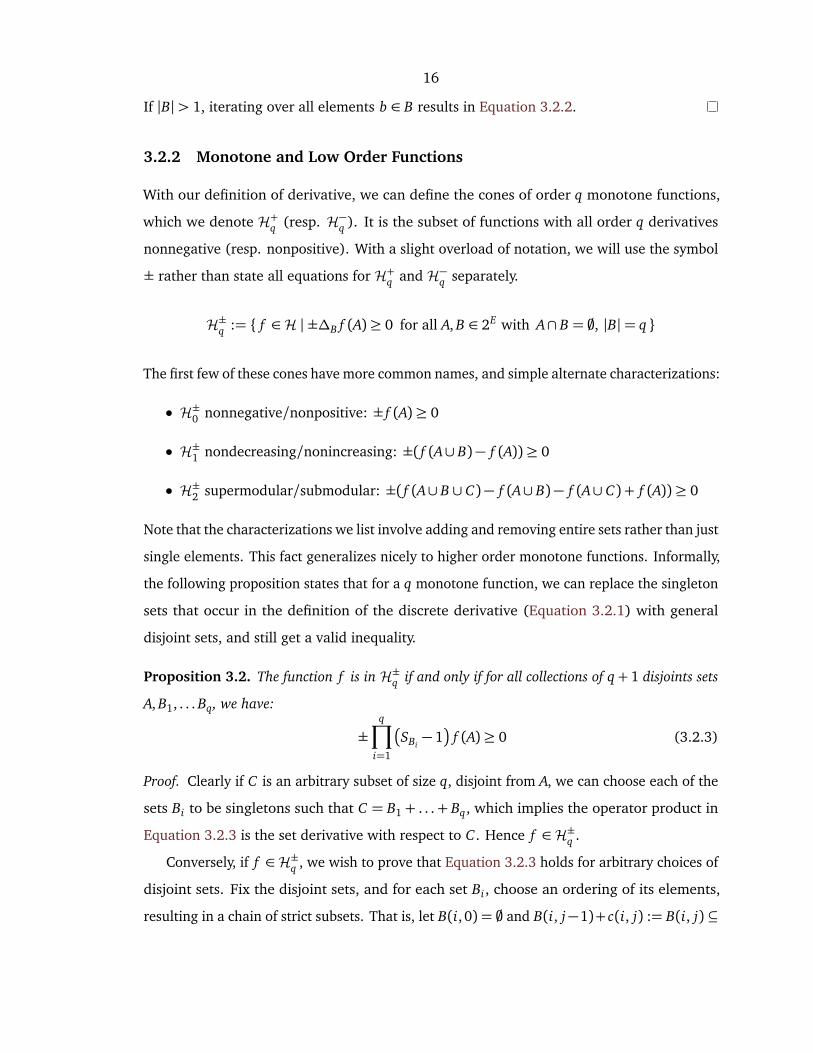
3.2.2 Monotone and Low Order Functions
With our definition of derivative, we can define the cones of order q monotone functions,
which we denote H+q (resp. H−q ). It is the subset of functions with all order q derivatives
nonnegative (resp. nonpositive). With a slight overload of notation, we will use the symbol
± rather than state all equations for H+q and H−q separately.
H±q := f ∈H | ±∆B f (A)≥ 0 for all A, B ∈ 2E with A∩ B = ;, |B|= q
The first few of these cones have more common names, and simple alternate characterizations:
• H±0 nonnegative/nonpositive: ± f (A)≥ 0
• H±1 nondecreasing/nonincreasing: ±( f (A∪ B)− f (A))≥ 0
• H±2 supermodular/submodular: ±( f (A∪ B ∪ C)− f (A∪ B)− f (A∪ C) + f (A))≥ 0
Note that the characterizations we list involve adding and removing entire sets rather than just
single elements. This fact generalizes nicely to higher order monotone functions. Informally,
the following proposition states that for a q monotone function, we can replace the singleton
sets that occur in the definition of the discrete derivative (Equation 3.2.1) with general
disjoint sets, and still get a valid inequality.
Proposition 3.2. The function f is in H±q if and only if for all collections of q+ 1 disjoints sets
A, B1, . . . Bq, we have:
±q∏
i=1
SBi− 1
f (A)≥ 0 (3.2.3)
Proof. Clearly if C is an arbitrary subset of size q, disjoint from A, we can choose each of the
sets Bi to be singletons such that C = B1 + . . .+ Bq, which implies the operator product in
Equation 3.2.3 is the set derivative with respect to C . Hence f ∈H±q .
Conversely, if f ∈H±q , we wish to prove that Equation 3.2.3 holds for arbitrary choices of
disjoint sets. Fix the disjoint sets, and for each set Bi, choose an ordering of its elements,
resulting in a chain of strict subsets. That is, let B(i, 0) = ; and B(i, j−1)+ c(i, j) := B(i, j) ⊆
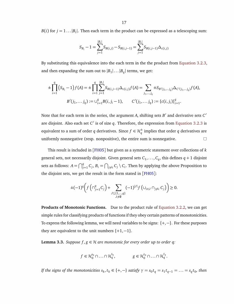
17
B(i) for j = 1 . . . |Bi|. Then each term in the product can be expressed as a telescoping sum:
SBi− 1=
|Bi |∑
j=1
SB(i, j) − SB(i, j−1) =|Bi |∑
j=1
SB(i, j−1)∆c(i, j)
By substituting this equivalence into the each term in the the product from Equation 3.2.3,
and then expanding the sum out to |B1| . . . |Bq| terms, we get:
±q∏
i=1
SBi− 1
f (A) = ±q∏
i=1
|Bi |∑
j=1
SB(i, j−1)∆c(i, j) f (A) =∑
j1,..., jq
±SB′( j1,... jq)∆C ′( j1,... jq) f (A),
B′( j1, . . . jq) := ∪qi=1B(i, ji − 1), C ′( j1, . . . jq) := c(i, ji)
qi=1.
Note that for each term in the series, the argument A, shifting sets B′ and derivative sets C ′
are disjoint. Also each set C ′ is of size q. Therefore, the expression from Equation 3.2.3 is
equivalent to a sum of order q derivatives. Since f ∈H±q implies that order q derivatives are
uniformly nonnegative (resp. nonpositive), the entire sum is nonnegative.
This result is included in [FH05] but given as a symmetric statement over collections of k
general sets, not necessarily disjoint. Given general sets C1, . . . , Cq, this defines q+ 1 disjoint
sets as follows: A=⋂q
j=1 C j, Bi =⋂
j 6=i C j \ Ci. Then by applying the above Proposition to
the disjoint sets, we get the result in the form stated in [FH05]:
±(−1)q
f
∩qj=1C j
+∑
J⊆1,...,qJ 6=;
(−1)|J | f
∪i∈J ∩ j 6=i C j
≥ 0.
Products of Monotonic Functions. Due to the product rule of Equation 3.2.2, we can get
simple rules for classifying products of functions if they obey certain patterns of monotonicities.
To express the following lemma, we will need variables to be signs: +,−. For these purposes
they are equivalent to the unit numbers +1,−1.
Lemma 3.3. Suppose f , g ∈H are monotonic for every order up to order q:
f ∈Hs00 ∩ . . .∩Hsq
q , g ∈Ht00 ∩ . . .∩Htq
q .
If the signs of the monotonicities sk, tk ∈ +,− satisfy γ = s0 tq = s1 tq−1 = . . . = sq t0, then

18
f g ∈Hγq.
Proof. Let B be any set of size q. We use the product rule (Equation 3.2.2) to take the
derivative of f g with respect to B. For simplicity we do not write the argument A, but assume
it is disjoint from B. Within the resulting sum, we use the factorization γ= sk tq−k:
γ∆B( f g) =∑
C∈2E
[[C ⊆ B]] γ(∆C f )(SC∆B\C g)
=q∑
k=0
∑
C∈2E
[[C ⊆ B, |C |= k]] (sk∆C f )(tq−kSC∆B\C g)
For |C | = k, we have sk∆C f ≥ 0 since f ∈ Hsk0 and tq−kSC∆B\C g ≥ 0 since f ∈ Htq−k
q−k and
|B \C | = q− k. So each term in the sum multiplies to a nonnegative sign. Thus γ∆B( f g)≥ 0
for arbitrary B of size q, so indeed f g ∈Hγq.
For example, if f is nonnegative, nondecreasing, submodular (H+0 ∩H+1 ∩H
−2 ), and g is
nonnegative nonincreasing submodular (H+0 ∩H−1 ∩H
−2 ), then the product f g is nonnegative
submodular H+0 ∩H−2 , but neither increasing nor decreasing in general. Another example
of Lemma 3.3 is that the cone of nonnegative, nondecreasing, supermodular functions
(H+0 ∩H+1 ∩H
+2 ) is closed under multiplication.
We define q-th order functions, as functions with all derivatives beyond order q equal to
zero.
Hq := f ∈H |∆B f (A) = 0 for all A, B ∈ 2E with |B|> q
It is easy to see from the definition that: Hq =H+q+1∩H−q+1 and Hq ⊂Hq+1. The set of zeroth
order functions are constant functions. In the context of set functions, first order functions
are known as modular, and admit the description: f (A) = f (;) +∑
a∈A( f (a)− f (;)).
3.2.3 Fourier Analysis of Set Functions
In this section, we briefly introduce the Fourier transform for set functions, but it is primarily
expanded upon in Chapter 6. The characters of the group 2E can be written as ψB(A) :=
(−1)|A∩B| since ψB(A1)ψB(A2) = (−1)|A1∩B|(−1)|A2∩B| = (−1)|(A1A2)∩B| =ψB(A1A2). These
oscillate between 1 and −1 when elements of particular set B are added or removed from the
argument. Thus, we define the Fourier tranform of a set function by taking the appropriately

19
normalized inner product with such functions:
bf (B) :=1
2|E|
∑
A∈2E
f (A)ψB(A)
This is an orthogonal transform, so though the inverse formula has a different normalization
constant, it is otherwise the same: f (A) =∑
B∈2E bf (B)ψB(A). One way to interpret the
Fourier coefficient for a set is that it is the average of all the derivatives with respect to that
set (modulo a factor of −1 for odd sets).
bf (B) =(−1)|B|
2|E\B|
∑
A∈2E
[[A⊆ E \ B]]∆B f (A) (3.2.4)
Next, we define convolutions of set functions:
f ∗ g(A) :=∑
B∈2E
f (A B)g(B)
This satisfies the standard properties of a convolution: Commutivity f ∗g = g∗ f , Associativity,
( f ∗ g) ∗ h= f ∗ (g ∗ h), Linearity (α f + β g) ∗ h= α( f ∗ h) + β(g ∗ h). Also, convolution in
the time domain is multiplication in the Fourier Domain, and vice-versa.
Öf ∗ g(B) = 2nbf (B)bg(B), Óf g(B) = (bf ∗ bg)(B).
The advantage of our definition for set function derivatives is that it is just a convolution.
That is, ∆C f = f ∗ g where g(A) = [[A⊆ C]] (−1)|A|+|C |, and 2nbg(B) = [[C ⊆ B]] (−2)|C |. So a
derivative can be treated as a sort of high-pass filter. After taking the derivative with respect to
C , all coefficients which are not subsets of C are zeroed out: Õ∆C f (B) = [[C ⊆ B]] (−2)|C | bf (B).
This gives us a formula to express a derivative as a sum of Fourier coefficents:
∆C f (A) = (−2)|C |∑
B∈2E
[[C ⊆ B]] bf (B)ψB(A) (3.2.5)
Another important linear operator that can be expressed as a convolution is the projection of
a function onto the space of low order functions. By Equation 3.2.4, the subspace Hq can be
characterized as those functions with Fourier transform supported only on sets of size up to

20
q. That is:
Hq = f ∈H | bf (B) = 0 for all |B|> q
The best q-th order approximation for a set function in an `2 sense is given by setting all higher
order Fourier coefficients to zero: g = arg ming ′∈Hq‖ f − g ′‖ ⇔ bg(B) = [[|B| ≤ q]] bf (B).
This is immediate from the fact that the Fourier transform is an isometry. See [HH92] and
[GMR00] for the formulas of this operation in terms of different function bases.
In elementary signal processing, the domains analyzed are the continuous/discrete
circle/line (Zn, [0,1], Z, or R). Exactly as there, (periodic) shifting, derivatives, and low
pass filtering can all be expressed as convolutions, so unsurprisingly these operations all
commute with each other.
3.2.4 Tensor Product Bases of Set Functions
In addition to the standard basis and the Fourier transform, there are several other useful
bases for representing set functions. For a thorough discussion, see [GMR00], but let us
review two of the more important ones. The feature common to all the bases that we present
is that they can be expressed easily through tensor products.
Möbius Transform and Boolean Polynomials. One way to represent set functions is as a
multilinear (a.k.a. polynomial) function over the Boolean cube p(x) = p0+ p1 x[1]+ p2 x[2]+
. . . p1...n x[1] . . . x[n]. This gives a simple way to interpolate a set function continuously
over the unit cube by letting the variable x take on values [0,1]n ⊂ Rn. In this case, the
interpolation is multilinear by convention since Booleans satisfy x2 = x , and so there is no
reason to include nonlinear terms such as x[i]2.
To calculate the coeffcient of a polynomial that represents a set function, we evaluate the
set function derivative at the empty set. A set function derivative is exactly the stencil of a
mixed derivative of an n dimensional function; an order q discrete derivative is the forward
difference operator tensored in some set of q dimensions. Since the Boolean polynomial
is multilinear, in general, set function derivatives equal the continuous partial derivatives
exactly (provided the argument set and derivative set are disjoint). For example: suppose
E = 1, 2, 3, and the set function f is related to the Boolean polynomial p by f (A) = p(1A).
Then the set function derivative with respect to the set 1, 2 evaluated at the set 3 equals the

21
mixed partial derivative of p at the corresponding corner: ∆12 f (3) = D12p(13) = p12 + p123.
The transformation from set function values to polynomial coefficients is sometimes
called the Möbius transform. We can express this not only as a set derivative, but also we
can use Equation 3.2.5 to equate it with a sum of Fourier coefficients.
g(B) =∆B f (;) = (−2)|B|∑
C
[[B ⊆ C]] bf (C)
f (A) =∑
B
[[B ⊆ A]] g(B)
Disjuction. Functions of the form min(1, |A∩ B|) are equivalent to a disjunction (Boolean
OR) operation. A sum of such functions is equivalent to a set cover function, as described in
subsection 4.4.2. These functions do not quite form a basis of H, since they all have f (;) = 0.
But by including a constant offset, we get a basis for H. The corresponding analysis and
synthesis formulas are:
h(B) = −∆B f (E) = −2|B|∆E\B bf (E)
f (A) = f (;) +∑
B
min(1, |A∩ B|)h(B)
There is an interesting consequence to the formula relating the set cover coefficients to Fourier
coefficients. The original function f is set cover representable (meaning it can be expressed
as a nonnegative combination of such functions, so that h(B)≥ 0 for all nonempty B) if and
only if the Fourier coefficients bf (B) for nonempty sets are nonpositive and nondecreasing.
Tensor Product Notation. The above formulas may seem a bit mysterious and hard to
check for correctness. However, the calculations are fairly simple if you consider set functions
as vectors in R2n, since all of the bases we have described can be expressed in terms of n-fold
tensor products of 2× 2 matrices. Let us denote (⊗n) for the operation of tensoring a matrix
with itself n times. Then the main formulas of this section can be written as:
Fourier: bf =
1/2 1/21/2 −1/2
⊗n
f , f =
1 11 −1
⊗nbf .
Möbius: g =
1 0−1 1
⊗n
f , f =
1 01 1
⊗n
g.

22
Disjunction: h= −
0 11 −1
⊗n
f , f = f (;) +
1 11 1
⊗n
−
1 11 0
⊗n
h.
Therefore, it is straightforward to derive the basic formulas relating different tensor product
bases by simply inverting and/or multiplying 2× 2 matrices.
3.3 Properties of Submodular Set Functions
There are many equivalent characterizations of submodularity. As we have already introduced
the notion of set derivative, we give a few which are directly related to set derivatives:
1. f (A+ b+ c)− f (A+ b)− f (A+ c) + f (A)≤ 0, for all b, c ∈ E, A⊆ E − b− c.
2. f (A∪ B ∪ C)− f (A∪ B)− f (A∪ C) + f (A)≤ 0, for all A, B, C disjoint.
3. f (A∩ B) + f (A∪ B)≤ f (A) + f (B) for all A, B ∈ 2E .
4. f (A+ c)− f (A)≥ f (B + c)− f (B) for all c ∈ E, A⊆ B ⊆ E − c.
There aren
2
2n−2 different inequalities to check in item 1. This is the minimum number of
inequalities needed to check submodularity in general. That is, no subset of these inequalities
implies any other subset of them. Theorem 3.2 gives the characterizations of items 2. The
interpretation of item 4 is that first order differences are decreasing functions. It is an easy
consequence of item 3. To test submodularity, it is generally easiest to use item 1. Besides
the fact that it has fewer inequalities to check, each inequality involves the change in value
when adding only 2 elements to a set.
These properties seem fairly similar in that they involve inequalities of the set derivatives.
However, there are several other characterizations, some of which appear to have nothing to
do with second order differences being negative. For example, a set function f is submodular
if and only if for all c ∈ Rn it holds that A, B ∈ Qc ⇒ A∩ B, A∪ B ∈ Qc, where Qc :=
arg minA f (A) + ⟨1A,c⟩. In words, this means that the collection of minimizers of f plus any
modular function is a lattice. See [Fuj05] for a proof. Another example of a rather striking
necessary and sufficient condition for submodularity is given in Proposition 3.4.
Maximization While the exact maximization of general submodular functions is a hard
problem, maximizing a nonnegative nondecreasing submodular function under a cardinality

23
constraint can be done to within a constant factor of the optimum. That is, if one wishes to
find a maximal set of size k, then a simple greedy algorithm2 will give a set of cardinality k
with function value no less than 1− 1/e of the maximal set of cardinality k [NWF78]. This
useful property of approximate maximization is is a major driving force behind the interest
in submodular functions, as it has many practical applications and useful generalizations.
However, aside from our experiments showcased in Figure 6.1, we otherwise focus on the
problem of submodular minimization.
3.3.1 Convex Analysis of Submodularity
We give an overview of how convex analysis can be used to analyze submodular functions.
While this presentation is original, the material is standard [Sch03, Fuj05, Bac11].
We start by defining some important polyhedra used in the analysis of submodular
functions. We can define the subdifferential of a set function in a form analogous to continous
functions, except modular set functions play the role of linear functionals. Any vector λ ∈ Rn
defines a modular function on E, which we can denote in different ways, depending on what
is convenient for the context:
2E 3 A 7→ λ(A) := ⟨1A,λ⟩=∑
a∈A
λ[a]
Then the subdifferential of a set function at a set is defined as a modular function which
lower bounds the change in value of the function relative to that set. That is, λ is subgradient
for f at the set A, if for all sets B the difference f (B)− f (A) is bounded below by difference
λ(B)−λ(A).
∂ f (A) := λ ∈ Rn | f (B)≥ f (A) + ⟨1B − 1A,λ⟩ for all B ∈ 2E
We also refer to this as the discrete subdifferential. Unlike a continuous subdifferential, which
may be empty if a function is nonconvex, the discrete subdifferential is always nonempty. In
fact, the subdifferential for the set A is unbounded along every ray in the direction 1A−1E\A.
This is true for any set function. This is because ∂ f (A) is a polyhedron defined by the normal
directions 1B − 1A where B ∈ 2E \ A, and for any such direction ⟨1B − 1A,1A− 1E\A⟩ =2Add elements one at a time by choosing whichever element increases the function the most.

24
−|A B| < 0. So moving far enough in the direction 1A − 1E\A will always result in a
subgradient. Precisely, for any λ ∈ Rn, we have:
λ+ t(1A− 1E\A) ∈ ∂ f (A) ⇔ t ≥maxB∈2E
B 6=A
f (A)− f (B) +λ(B)−λ(A)|A B|
In what follows, we will assume that the set function f is ‘normalized’, it has f (;) = 0,
possibly by subtracting an offset. The submodular polyhedron Pf and base polytope B f are
thus defined by:
Pf := λ ∈ Rn | ⟨1A,λ⟩ ≤ f (A) for all A∈ 2E (3.3.1)
B f := λ ∈ Rn | ⟨1,λ⟩= f (E), and ⟨1A,λ⟩ ≤ f (A) for all A∈ 2E (3.3.2)
It is easy to see that that Pf = ∂ f (;). Furthermore,
Pf ∩ ∂ f (A) = Pf ∩ λ ∈ Rn | λ(A) = f (A)
In particular, B f = ∂ f (;)∩ ∂ f (E). Note that all vectors in the set B f must satisfy λ[a]≤ f (a)
and ⟨1,λ⟩= f (E), and thus λ[b]≥ f (E)−∑
a∈E−b f (a). So the set B f is bounded and we
are justified in referring to it as a polytope. The elements of the base polytope are called
the bases of the function. Note when f is the rank function of a matroid (cf. Appendix A),
each extreme point of the base polytope corresponds to the indicator vector of a base (a.k.a.
basis) for the matroid.
The base polytope essentially contains all the subgradients needed to fully characterize a
submodular function. While it is defined by exponentially many constraints, there is a simple
formula to optimize a linear function over it if we have oracle access to the function, if and
only if the function is submodular. The key insight due to Edmonds [Edm70] is that solving
maxλ∈B f⟨x,λ⟩ depends only on the ordering of the components of x.
We say that a permutation π ∈ Sn (Sn is the nth symmetric group, the set of all bijections
from E to itself) is consistent with a vector x, if the components of x are nonincreasing with
respect to that permutation. Let Kπ be the cone of all vectors consistent with π, and Kπ be

25
its polar cone.
Kπ := x ∈ Rn | x[π1]≥ x[π2] . . .≥ x[πn] (3.3.3)
Kπ := λ ∈ Rn | ⟨1,λ⟩= 0, and∑k
i=1λ[πi]≤ 0 for k = 1 . . . n (3.3.4)
Note that these cones are proper with respect to the subspace of vectors orthogonal to 1.
Given a permutation π, consider a sequence of sets starting with the empty set, adding
one element at a time in the order specified by π. Then for a set function f , define νπ, f ∈ Rn
to be the vector with coordinates equal to the changes in value of f over this sequence of
sets. For this, it will be useful to define $k to be the subset of E consisting of the first k
elements in π.
νπ, f [πk] :=∆πkf ($k−1) = f ($k)− f ($k−1) (3.3.5)
$k := π1, . . . ,πk (3.3.6)
The points νπ, f are called the extreme bases of the function f ; we will justify the name by
proving that they are indeed the vertices of the base polytope. First, we need to prove that
they are even in the base polytope.
Proposition 3.4. The set function f is submodular if and only if νπ, f ∈ B f for all π ∈ Sn.
Proof. Suppose f is not submodular. Then f (A+ b + c) + f (A) > f (A+ b) + f (A+ c) for
some b, c ∈ E, A⊆ E − b− c. Let π be a permutation with $k = A, A+ b, A+ b+ c for k =
|A|, |A|+1, |A|+2 respectively. This means ⟨1A,νπ, f ⟩ = f (A), νπ, f [c] = f (A+ b+ c)− f (A+ b)
and thus:
⟨1A+c,νπ, f ⟩= ⟨1A,νπ, f ⟩+ ⟨1c,νπ, f ⟩= f (A) + f (A+ b+ c)− f (A+ b)> f (A+ c)
So we conclude νπ, f violates a constraint and is not in the polytope B f .
Otherwise, suppose f is submodular. Clearly ⟨1,νπ, f ⟩ = f (E) for all permutations π,
so the equality constraint in the definition of B f is satisfied. Let A be any set and π be any
permutation. We wish to show that ⟨1A,νπ, f ⟩ ≤ f (A). Let the increasing sequence k(·) corre-
spond to the indices of A relative to the permutation π. That is, A= πk(1),πk(2), . . . ,πk(|A|).

26
This means we have for j = 1 . . . |A|, A∩$k( j)−1 = πk(1),πk(2), . . . ,πk( j−1)= A∩$k( j−1).
⟨1A,νπ, f ⟩=|A|∑
j=1
f ($k( j))− f ($k( j)−1)
≤|A|∑
j=1
f (A∩$k( j))− f (A∩$k( j)−1) (submodularity)
=|A|∑
j=1
f (A∩$k( j))− f (A∩$k( j−1)) (definition of k(·))
= f (A∩$k(|A|)) = f (A)
So we conclude ⟨1A,νπ, f ⟩ ≤ f (A) for all A∈ 2E so νπ, f ∈ B f .
Note that Proposition 3.4 gives yet another characterization of submodularity. For the
rest of this section, we will assume that f is submodular. Having established that the points
defined by Equation 3.3.5 are bases, we can characterize them further:
Proposition 3.5. The point νπ, f is the unique element of B f which maximizes the inner product
with any element of Kπ.⋂
x∈Kπ
arg maxλ∈B f
⟨x,λ⟩=
νπ, f
Furthermore, νπ, f is extreme in B f .
Proof. First we show that νπ, f is maximal when x is a corner of the unit cube. Let A
be any set such that 1A ∈ Kπ. That is, A = $k for k = |A|. Note that by definition
of B f , the maximal value maxλ∈B f⟨1A,λ⟩ must be no more than f (A). By construction,
⟨1$k ,νπ, f ⟩ =∑k
j=1 f ($ j)− f ($ j−1) = f ($k) = f (A), so νπ, f achieves this maximum value.
By Proposition 3.4, νπ, f is an element of B f . So we conclude νπ, f ∈ arg maxλ∈B f⟨1$k ,λ⟩
for k = 1 . . . n.
Next, suppose x is an arbitrary point in Kπ. Then we can decompose it into a sum:
x= x[πn]1+∑n−1
k=1αk1$k with nonnegative coefficients αk = x[πk]− x[πk+1]≥ 0. Since
⟨1,λ⟩ is constant over B f , and νπ, f is maximal for each term in the sum, we conclude that
νπ, f ∈ arg maxλ∈B f⟨x,λ⟩.
To show uniqueness, suppose λ,λ′ ∈ B f both maximize the inner product for all x ∈ Kπ.
Then ⟨x,λ⟩ ≤ ⟨x,λ′⟩ for all x ∈ Kπ, which is equivalent to λ−λ′ ∈ Kπ. Likewise, λ′−λ ∈ Kπ,

27
but since Kπ is pointed, this implies that λ= λ′.
Similarly, to see that νπ, f is extreme in B f , suppose that νπ, f = θλ1 + (1 − θ)λ2 for
some λ1,λ2 ∈ B f , with θ ∈ (0,1). The optimality of νπ, f implies that ⟨x,λ2⟩ ≤ ⟨x,νπ, f ⟩
for all x ∈ Kπ, which is equivalent to λ2 − νπ, f = θ(λ1 − λ2) ∈ Kπ. Likewise λ1 − νπ, f =
(1−θ )(λ2−λ1) ∈ Kπ. Again by using the fact that Kπ is a pointed cone, we have λ2−λ1 = 0,
and thus νπ, f = λ1 = λ2.
So we have justified the name extreme base for the vectors νπ, f . In fact, these are the
only extreme elements of B f . That is, we can characterize the base polytope as the convex
hull of the collection νπ, f π∈Sn.
Proposition 3.6. B f = conv νπ, f π∈Sn.
Proof. Clearly every x ∈ Rn is contained in some cone Kπ. Thus Proposition 3.5 implies
that maxλ∈B f⟨x,λ⟩ = maxπ∈Sn
⟨x,νπ, f ⟩ for all x ∈ Rn. So if C = conv νπ, f π∈Sn, we have
σB f= σC everywhere. Both sets are closed and convex, thus δB f
= σ∗B f= σ∗C = δC , so we
conclude they are identical.
3.3.2 Lovász Extension
Let us review what we have established about σB f, the support function of the base polytope
of f . First, what does it evaluate to at a corner of the unit cube? By Proposition 3.4, the
points νπ, f are contained in the base polytope, therefore for any set A∈ 2E , the inequality
⟨1A,λ⟩ ≤ f (A) is satisfied with equality for some λ ∈ B f (namely any νπ, f for which
1A ∈ Kπ). Thus σB f(1A) = maxλ∈B f
⟨1A,λ⟩ = f (A). So therefore σB fis an interpolation of
f to the vertices of the unit cube. Furthermore, since it is a support function, it is convex
by construction, making it a natural tool for use in minimization. Since this function is so
important, we will denote it simply f , and we refer to it as the Lovász extension of f .
f (x) := σB f(x) =max
λ∈B f
⟨x,λ⟩
On a historical note, this is named after Lovász, who was the first to consider it as a tool
for minimization [GLS81, Lov83]. It appeared earlier in the work of Edmonds [Edm70]
implicitly, in that he showed how maximizing a linear function over the base polytope can be
done in a greedy fashion.

28
Since B f is bounded, f has full domain. The subgradient of the Lovász extension at a
point x is the convex hull of all base vertices for permutations consistent with that vector:
∂ f (x) = conv νπ, f | x ∈ Kπ (3.3.7)
In particular, the subgradients at a corner of the unit cube are also discrete subgradients for
f .
∂ f (A)∩ B f = conv νπ, f | A= π1, . . . ,π|A| (3.3.8)
Consider what Equation 3.3.7 implies about the relationship between subdifferentials at
different points. If the point y is consistent with at least the permutations with which x is
consistent, then all subgradients at x are also subgradients at y:
x ∈ Kπ for all π such that y ∈ Kπ⇒ ∂ f (x) ⊆ ∂ f (y)
In particular, by relating the subdifferential of x to the corner point 1A, we can derive a
condition for when the continous subgradients for f are also discrete subgradients for f .
Given a point x, defining X+α to be the subset of components of x greater than or equal to α,
it is not hard to see that x ∈ Kπ if and only if 1X+α∈ Kπ for all α ∈ R. So by Equation 3.3.7,
we get:
X+α := e ∈ E | x[e]≥ α
∂ f (x) =⋂
α∈R∂ f (X+α )∩ B f (3.3.9)
Note that there is a subtlety to this characterization that is important for algorithms that use
the Lovász extension to minimize the set function. In order to conclude that the continuous
subdifferential ∂ f (x) is included in the set function subdifferential ∂ f (A), it is necessary
that the components of x in A be strictly separated from the complementary components.
mina∈A
x[a]> maxb∈E\A
x[b] ⇒ ∂ f (x) ⊆ ∂ f (A) (3.3.10)
mina∈A
x[a]≥ maxb∈E\A
x[b] ; ∂ f (x) ⊆ ∂ f (A) (3.3.11)
Note that the premise of Equation 3.3.11 does imply that ∂ f (x)∩ ∂ f (A) is nonempty.

29
3.3.3 Examples of Base Polytopes
Which is more important—a submodular function or its base polytope? Of course, given
the dual relationship between the two, one cannot really be more important than the other,
but historically, base polytopes were discovered first by Edmonds. Any base polytope is the
union of the faces of a polymatroid. (Interestingly, polymatroids can be defined without
mentioning submodularity.)
We start with a short proof of an important property of submodular functions. For any
submodular function, minimizing out a subset of the variables results in another submodular
function. This is exactly analogous to convex functions. Suppose a the function g(A, B) is a
submodular function on 2E×F , where A∈ 2E , B ∈ 2F . Then suppose f is given by minimizing
g over all arguments B:
f (A) =minB⊆F
g(A, B) (3.3.12)
It is simple to show if g is submodular, then f must be as well:
f (A1) + f (A2) = g(A1, B1) + g(A2, B2) Where Bi = arg minB⊆F
g(Ai, B)
≥ g(A1 ∪ A2, B1 ∪ B2) + g(A1 ∩ A2, B1 ∩ B2) (Submodularity of g)
≥ f (A1 ∪ A2) + f (A1 ∩ A2) (Minimality of f )
In particular, when a function f is graph representable, it can be written as a minimum over
submodular g(A, B), where g is a fully general quadratic function.
f (A) = c(A) +minB
s(B) + 1TA W111E\A+ 1TA W121F\B + 1
TB W221F\B
The term graph representable refers to the fact that a second-order submodular function is
a cut function of a graph. We can express points in the base polytope of f through 2|E|+|F |
linear inequalities. That is, λ ∈ B f if:
−1TA (λ− c) + sT1B + 1TA W111E\A+ 1
TA W121F\B + 1
TB W221F\B ≥ 0
for all A∈ 2E , B ∈ 2F .
Now consider a simpler case where all entries of W11 and W22 equal zero. This means the

30
graph is bipartite: one partition for E and and the other for the variables to be minimized
over. Such a function can then be expressed as:
f (A) = 1TA c+minB
1TA W(1− 1B) + sT1B
= c(A) +∑
j
min(s j,w j(A))
For this function, we can introduce new variables to give a simple description of the base
polytope. That is, λ ∈ B f if there exists some Y ∈ R|E|×|F | such that:
λ= c+ YT1, 0≤ Y≤W, Y1= s.
So testing membership in this base polytope is much simpler than the general case. What
happens if we iterate Equation 3.3.12, by introducing a new bipartite graph between sets of
variables. If we do this k times, we get a graph representable function, only now the graph
is a trellis with k levels:
f (A) = 1TA c+ minB1,...Bk
1TA W1(1− 1B1) +
k∑
j=2
1TB j−1W j(1− 1B j
) + sT1Bk(3.3.13)
Again, this function has an efficiently representable base polytope. That is, we have λ ∈ B f
if for some matrices Y1, . . . ,Yk, we have:
λ= c+ YT1 1, 0≤ Y1 ≤W1, (3.3.14)
Y j1= YTj+11, 0≤ Y j+1 ≤W j+1 for j = 1 . . . k− 1,
Yk1= s.
3.4 Submodular Minimization
The general problem we are interested in is finding a global minimizer of a submodular
function. Finding Before discussing specific algorithmic techniques, let us review what the
optimality conditions and duality gap are for solving submodular minimization as a convex
minimization problem. Recall that σ[0,1]n(x) =maxλ∈[0,1]n⟨x,λ⟩=∑
e∈E max(x[e], 0) is the
support function of the unit cube.
31
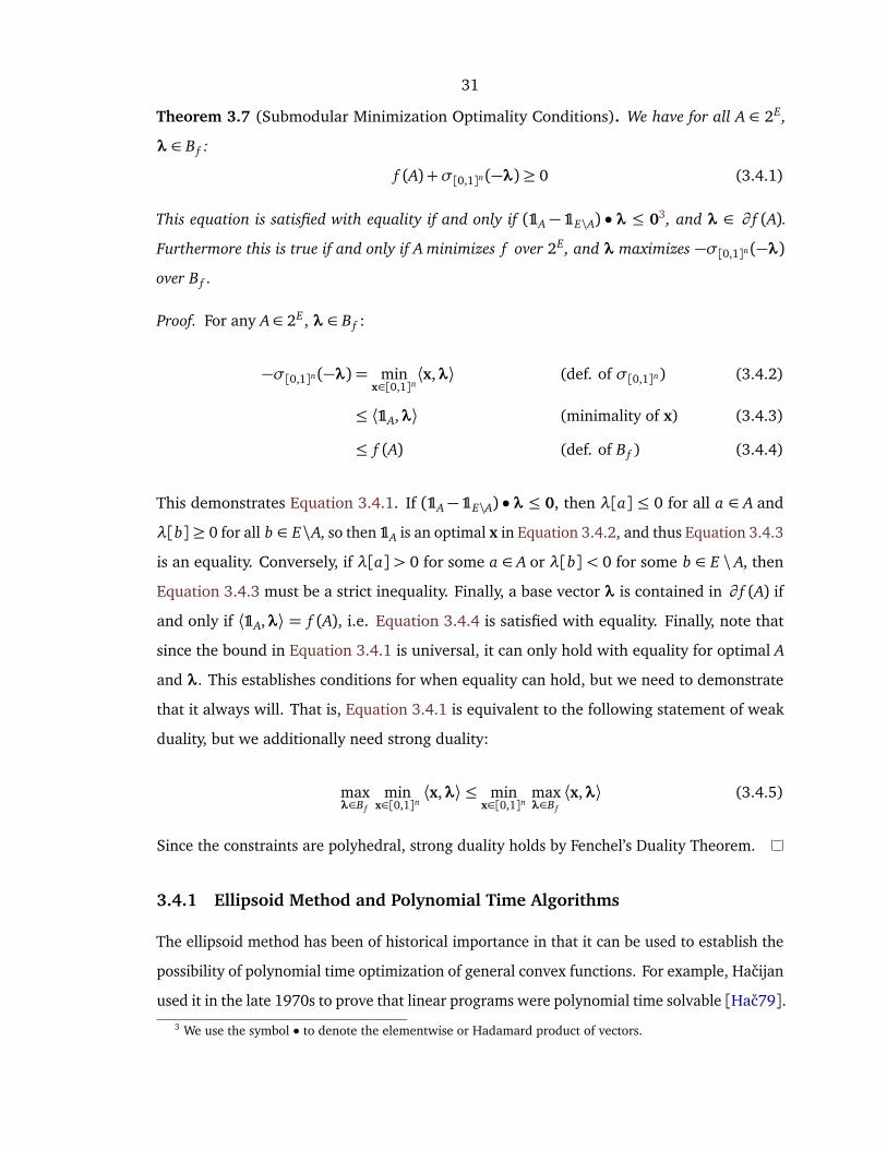
Theorem 3.7 (Submodular Minimization Optimality Conditions). We have for all A ∈ 2E ,
λ ∈ B f :
f (A) +σ[0,1]n(−λ)≥ 0 (3.4.1)
This equation is satisfied with equality if and only if (1A − 1E\A) • λ ≤ 03, and λ ∈ ∂ f (A).
Furthermore this is true if and only if A minimizes f over 2E , and λ maximizes −σ[0,1]n(−λ)
over B f .
Proof. For any A∈ 2E , λ ∈ B f :
−σ[0,1]n(−λ) = minx∈[0,1]n
⟨x,λ⟩ (def. of σ[0,1]n) (3.4.2)
≤ ⟨1A,λ⟩ (minimality of x) (3.4.3)
≤ f (A) (def. of B f ) (3.4.4)
This demonstrates Equation 3.4.1. If (1A− 1E\A) • λ ≤ 0, then λ[a] ≤ 0 for all a ∈ A and
λ[b]≥ 0 for all b ∈ E\A, so then 1A is an optimal x in Equation 3.4.2, and thus Equation 3.4.3
is an equality. Conversely, if λ[a] > 0 for some a ∈ A or λ[b] < 0 for some b ∈ E \ A, then
Equation 3.4.3 must be a strict inequality. Finally, a base vector λ is contained in ∂ f (A) if
and only if ⟨1A,λ⟩ = f (A), i.e. Equation 3.4.4 is satisfied with equality. Finally, note that
since the bound in Equation 3.4.1 is universal, it can only hold with equality for optimal A
and λ. This establishes conditions for when equality can hold, but we need to demonstrate
that it always will. That is, Equation 3.4.1 is equivalent to the following statement of weak
duality, but we additionally need strong duality:
maxλ∈B f
minx∈[0,1]n
⟨x,λ⟩ ≤ minx∈[0,1]n
maxλ∈B f
⟨x,λ⟩ (3.4.5)
Since the constraints are polyhedral, strong duality holds by Fenchel’s Duality Theorem.
3.4.1 Ellipsoid Method and Polynomial Time Algorithms
The ellipsoid method has been of historical importance in that it can be used to establish the
possibility of polynomial time optimization of general convex functions. For example, Hacijan
used it in the late 1970s to prove that linear programs were polynomial time solvable [Hac79].3 We use the symbol • to denote the elementwise or Hadamard product of vectors.

32
While its generality is a great strength for proving theorems, in practice the problems it can
be applied to have specialized methods that work much faster.
Suppose we wish to minimize a convex function using an oracle which takes as input
any point in the function’s domain and returns the function value and a subgradient. We
can use the fact that for any current iterate xk with subgradient λk ∈ ∂ f (xk), a minimizer
x∗ ∈ arg min f must be contained in the half-space ⟨x∗,λk⟩ ≤ ⟨xk,λk⟩+ f kbest − f (xk), where
f kbest is the smallest value of f encountered up to step k. Splitting algorithms are a general
class of algorithms that maintain a feasible region such as a polytope or an ellipsoid, then
use oracle information to splits the feasible region and reduce it somehow.
In particular, a simple variant of the ellipsoid algorithm might proceed as follows. Start
with ellipsoid E0 large enough to be guaranteed to contain a minimizer of f , set k = 0
and begin: Let xk be the the centroid of Ek, and use the oracle to get a subgradient λk ∈
∂ f (xk). This gives a half-space that splits the current ellipsoid, namely Hk := x ∈ Rn |
⟨x,λk⟩ ≤ ⟨xk,λk⟩+ f kbest − f (xk) . Let Ek+1 be the ellipsoid of minimal volume which contains
the intersection Hk∩Ek. Increment k and repeat these iterations until an iterate is sufficiently
close to optimality.
To represent ellipsoids numerically, one can use a positive definite matrix and a vector.
Under this representation, computing the minimal volume ellipsoid for the next iterate
amounts to a rank-one update rule of the matrix. The algorithm can be analyzed by bounding
the rate at which the volume of these ellipsoids decrease.
The Lovász extension f is a convex function, and by Equation 3.3.7, a subgradient at any
point can be generated efficiently, provided evaluation of the set function f is efficient. So one
can use a generic convex minimization algorithm such as an ellipsoid method to minimize
f over the unit cube. Note that the original ellipsoid method proposed for submodular
minimization in [GLS81] differs somewhat from the algorithm outlined above, but the
important ideas are the same: using the convexity of f and an efficient subgradient oracle to
minimize the set function.
However, the asymptotic running time of the ellipsoid method depends on the values of
the function itself, not just the size of the problem. Hence its running time is actually weakly
polynomial. Since then, several strongly polynomial algorithms for submodular minimization
have been developed. [IFF01] [IO09] Unfortunately, these are all of complexity at least
O(n5), and they are not empirically fast enough to be of practical use for all but very small

33
problems.
3.4.2 Fujishige’s Minimal Norm Algorithm
As originally shown by Fujishige [FI11], finding the point of the base polytope B f of minimal
`2 norm is equivalent to solving the submodular minimization problem. (We prove a more
general version of this equivalance in Theorem 5.4.)With access to an oracle that maximizes a
linear function over a basepolytope, one uses the Frank-Wolfe algorithm to find the minimum
norm point in that polytope. The algorithm is guaranteed to converge in finite time because
there are only finitely many possible subsets of vertices, and it is a descent algorithm which
never returns to the same state. In general the algorithm could require exponentially many
calls to an oracle, albeit no problem instance exhibiting this behavior is known.
To satisfy the role of the oracle, we need an an efficient subroutine which can solve
arg maxλ∈B f⟨x,λ⟩ for any x ∈ Rn. By Proposition 3.5, we know that if x ∈ Kπ, the point
νπ, f is a maximizing vertex of the polytope for that functional. So, we just need to sort4
the components of x to find a permutation with which x is consistent, and then our oracle
returns the base vertex given by the formula in Equation 3.3.5. This procedure is known
as the greedy algorithm, because if f is the rank function of a matroid, it is equivalent to
adding elements to an independent set greedily depending on their weight x[e].
Despite there being no subexponential upper bounds on the running time, this algorithm
works quite well in practice. The exact performance will depend some subtleties, such as
how expensive it is to compute the submodular function. If f is a complicated function such
as a log-determinant, then computing νπ, f given π may actually be the bottleneck of the
program.
3.4.3 Special Cases
There are certain special cases of submodular minimization for which faster algorithms are
known to exist. Even these are not necessarily useful in practice, but they are always asymp-
totically faster than the algorithms which make no assumptions other than submodularity.
4This can be a major source of nondeterminacy in an implementation if a sorting routine does not specify howties are broken. Ties are not unlikely because the minimum norm base is expected to have many components ofthe same magnitude.

34
Symmetric Unconstrained minimization of a symmetric submodular function is trivial,
since for such functions we have 2 f (;) = f (;) + f (E) ≤ f (A) + f (E \ A) ≤ 2 f (A) for all A,
so ; and E trivially minimize A. However, if we restrict the search domain to exclude the
extreme sets, the minimization problem is very much of interest. In this case, we can use
an algorithm discovered by Queyranne [Que98] to minimize the a symmetric submodular
function over the range 2E \ ;, E.
Quadratic Potentials and Extensions The minimization of second-order submodular func-
tions can be reformulated as finding the smallest cut of a graph with positive edge weights
which separates two specific vertices. This is dual to finding the maximum flow between those
two vertices, if the edge weights are capacities. This is a classic problem in computer science
and there are a great variety of algorithms for solving it efficiently. One of the conceptually
simplest of these is the Ford-Fulkerson algorithm which, in its simplest form, requires the
weights to be integral.
Yet, even if a submodular function is not second order, it may still be possible to use
min-cut/max-flow algorithms to minimize it. This is done by introducing extra Boolean
variables to create a higher dimensional second order function, such that the original function
is given by minimizing the second order function over the extra variables. Functions that
admit such a representation are called graph representable. Much work has been done over
the years to determine which functions are graph representable, and, furthermore, how to
most efficiently represent the function, or at least approximate it efficiently. See for example,
[KZ04], [JLB11]. Graph representable functions are necessarily submodular.

35
Chapter 4
Smoothed Gradient Methods forDecomposable Functions
4.1 Introduction
Several submodular minimization problems arising in machine learning and other domains
have structure that allows for solving them more efficiently. Examples include symmetric
functions that can be solved in O(n3) evaluations using Queyranne’s algorithm [Que98],
and functions that decompose into attractive, pairwise potentials, that can be solved using
graph cutting techniques [FD05]. In this chapter, we introduce a novel class of submodular
minimization problems that can be solved efficiently with convex optimization. In particular,
we develop an algorithm SLG, that can minimize a class of submodular functions that we call
decomposable. These are functions that can be decomposed into sums of concave functions
applied to modular (additive) functions. Our algorithm is based on recent techniques of
smoothed convex minimization [Nes05] applied to the Lovász extension. We demonstrate
the usefulness of our algorithm on a joint classification-and-segmentation task involving
tens of thousands of variables, and show that it outperforms state-of-the-art algorithms for
general submodular function minimization by several orders of magnitude.
4.2 Background on Submodular Function Minimization
We are interested in minimizing set functions that map subsets of some base set E to real
numbers; i.e. given f : 2E → R we wish to solve for A∗ ∈ arg minA f (A). For simplicity of
notation, we use the base set E = 1, . . . n, but in an application the base set may consist of
nodes of a graph, pixels of an image, etc. Without loss of generality, we assume f (;) = 0. If

36
the function f has no structure, then there is no way solve the problem other than checking
all 2n subsets. In this chapter, we consider functions that satisfy a key property that arises in
many applications: submodularity (c.f., [Lov83]). A set function f is called submodular if
and only if, for all A, B ∈ 2E , we have
f (A∪ B) + f (A∩ B)≤ f (A) + f (B). (4.2.1)
Submodular functions can alternatively, and perhaps more intuitively, be characterized in
terms of their discrete derivatives. First, we define ∆c f (A) = f (A∪ c)− f (A) to be the
discrete derivative of f with respect to c ∈ E at A; intuitively this is the change in f ’s value
by adding the element c to the set A. Then, f is submodular if and only if:
∆c f (A)≥∆c f (B), for all A⊆ B ⊆ E − c.
Note the analogy to concave functions; the discrete derivative is smaller for larger sets, in
the same way that φ(x +h)−φ(x)≥ φ(y +h)−φ(y) for all x ≤ y, h≥ 0 if and only if φ is
a concave function on R. Thus a simple example of a submodular function is f (A) = φ(|A|)
where φ is any concave function. Yet despite this connection to concavity, minimizing a
submodular function can be done in polynomial time, wheras maximizing it is NP-hard.
This is similar to the fact that it is easier to minimize a convex function than to maximize.
One explanation for this is that submodular minimization can be reformulated as a convex
minimization problem.
To see this, consider taking a set function minimization problem, and reformulating it as
a minimization problem over the unit cube [0, 1]n ⊂ Rn. Define 1A ∈ Rn to be the indicator
vector of the set A, i.e.,
1A[e] =
0 if e /∈ A
1 if e ∈ A
We use the notation x[e] for the component of the vector x corresponding to element e. Also
we drop brackets and commas in subscripts, so 1ab = 1a,b and 1a = 1a. For any vector
λ ∈ Rn, we use the shorthand λ(A) for the corresponding modular function:
λ(A) :=∑
a∈A
λ[a] = ⟨1A,λ⟩

37
A continuous extension of a set function is a function with a continuous argument that
interpolates the values of the set function to the corners of the unit cube. That is, we should
have [0, 1]n ⊆ dom f ⊆ Rn and f (A) = f (1A). Furthermore, we do not want the minimum of
the continous function to be completely unrelated to the minimum of the set function. That
is, if a particular set is a minimizer of the set function, then that should necessarily imply
that the corresponding indicator vector is a minimizer of the continous extension over the
unit cube:
A∗ ∈ arg minA∈2E
f (A) ⇒ 1A∗ ∈ arg minx∈[0,1]n
f (x). (4.2.2)
A key result due to Lovász [Lov83] states that each submodular function f has an extension
f that not only satisfies the above property, but is also convex and efficient to evaluate. We
can define the Lovász extension in terms of the base polytope B f :
f (x) =maxλ∈B f
⟨λ,x⟩, B f = λ ∈ Rn | λ(E) = f (E), λ(A)≤ f (A), for all A∈ 2E .
The base polytope B f is defined by exponentially many inequalities, and evaluating f requires
solving a linear program over this polyhedron. Perhaps surprisingly, as shown by Lovász, f
can be very efficiently computed as follows. For a fixed x ∈ Rn, let π: E→ E be a permutation
such that x[π1]≥ . . .≥ x[πn], and then define the set$k = π1, . . . ,πk. Then we have a
formula for f and a subgradient:
f (x) =n∑
k=1
x[πk]( f ($k)− f ($k−1)), ∂ f (x) 3
n∑
k=1
1πk( f ($k)− f ($k−1)). (4.2.3)
Note that if two components of x are equal, the above formula for f is independent of the
permutation chosen, but the subgradient is not unique.
Equation 4.2.2 was used to show that submodular minimization can be achieved in
polynomial time [Lov83]. However, algorithms which directly minimize the Lovász extension
are regarded as impractical. Despite being convex, the Lovász extension is non-smooth, and
hence a simple subgradient descent algorithm would need O(1/ε2) steps to achieve O(ε)
accuracy.
Recently, Nesterov showed that if knowledge about the structure of a particular non-
smooth convex function is available, it can be exploited to achieve a running time of O(1/ε)

38
[Nes05]. One way this is done is to construct a smooth approximation of the non-smooth
function, and then use an accelerated gradient descent algorithm which is highly effective
for smooth functions. Connections of this work with submodularity and combinatorial
optimization are also explored in [CN07] and [Bac10]. In fact, in [Bac10], Bach shows that
computing the smoothed Lovász gradient of a general submodular function is equivalent
to solving a submodular minimization problem. In this chapter, we do not treat general
submodular functions, but rather a large class of submodular minimization functions that
we call decomposable. (To apply the smoothing technique of [Nes05], special structural
knowledge about the convex function is required, so it is natural that we would need special
structural knowledge about the submodular function to leverage those results.) We further
show that we can exploit the discrete structure of submodular minimization in a way that
allows terminating the algorithm early with a certificate of optimality, which leads to dramatic
performance improvements.
4.3 The Decomposable Submodular Minimization Problem
In this chapter, we consider the problem of minimizing submodular functions of the following
form:
f (A) = c(A) +∑
j
φ j(w j(A)), (4.3.1)
where c,w j ∈ Rn and w j ≥ 0 and φ j : [0,w j(E)]→ R are arbitrary one-dimensional concave
functions. Without loss of generality, we will assume, by rescaling if necessary, that ‖w j‖∞ = 1.
It is shown in 4.4.1 that functions of this form are submodular. We call this class of functions
decomposable submodular functions, as they decompose into a sum of concave functions
applied to nonnegative modular functions. Below, we give examples of decomposable
submodular functions arising in applications.
We first focus on the special case where all the concave functions φ j are positive multiples
of threshold functions min(τ, ·) for some threshold τ > 0. Since these functions are of key
importance, we denote Ψ(τ,w, A) to be the submodular function given by thresholding the
modular function w(A) at threshold τ:
Ψ(τ,w, A) :=min(τ,w(A))

39
We refer to these submodular functions as threshold potentials. In Section 4.6, we will show
how to generalize our approach to arbitrary decomposable submodular functions.
Examples. The simplest example is a 2-potential, which has the form φ(|A∩b, c|), where
φ(1) − φ(0) ≥ φ(1) − φ(2). It can be expressed as a sum of a modular function and a
threshold potential:
φ(|A∩ b, c|) = φ(0) + (φ(2)−φ(1))⟨1A,1bc⟩+ (2φ(1)−φ(0)−φ(2))Ψ(1,1bc, A)
An example application where such function arises is in image classification schemes such as
in [SWRC09]. In order to compute the Maximum a Posteriori configuration of a pairwise
Markov Random Field model, one must minimize a sum of these potentials. On a high level,
such an algorithm computes a value p[b] that corresponds to the log-likelihood of pixel b
being of one class vs. another, and for each pair of adjacent pixels, a value rbc related to the
log-likelihood that pixels b and c are of the same class. Then the algorithm classifies pixels
by minimizing a sum of 2-potentials: f (A) = c(A) +∑
b,c rbc(1− |1− ⟨1A,1bc⟩|). If the value
rbc is large, this encourages the pixels b and c to be classified similarly.
More generally, consider a higher order potential function: a concave function of the
number of elements in some activation set D, φ(|A∩D|) where φ is concave. It can be shown
that this can be written as a sum of a modular function and a positive linear combination
of |D| − 1 threshold potentials with boolean weights (w j ∈ 0,1n). However, threshold
potentials with nonuniform weights are strictly more general than those with boolean weights.
That is, there exists τ and w such that Ψ(τ,w, A) cannot be expressed as∑
jφ j(|Dj ∩ A|) for
any collection of concave φ j and sets Dj.
Recent work [KLT09] has shown that classification performance can be improved by
adding terms corresponding to such higher order potentials φ j(|Dj ∩ A|) to the objective
function where the functions φ j are piecewise linear concave functions, and the regions Dj
of various sizes generated from a segmentation algorithm. Minimization of these particular
potential functions can then be reformulated as a graph cut problem [KKT07], but this is
less general than our approach.
Another canonical example of a submodular function is a set cover function. Such a
function can be reformulated as a combination of threshold potentials with boolean weights

40
and unit threshold (details in 4.4.2). Thus all functions that are weighted combinations of
set cover functions can be expressed as threshold potentials.
Another example of decomposable functions arises in multiclass queuing systems [II07].
These are of the form f (A) = u(A)φ(v(A)), where u,v are nonnegative weight vectors and
φ is a nonpositive nonincreasing concave function. We show in 4.4.3, that with the proper
choice of φ j and w j, this can in fact be reformulated as sum of the type in Equation 4.3.1
with n terms.
In our own experiments, shown in Section 4.7, we use an implementation of TextonBoost
[SWRC09] and augment it with quadratic higher order potentials. That is, we use TextonBoost
to generate per-pixel scores c, and then minimize f (A) = c(A) +∑
j |A∩ Dj||Dj \ A|, where
the regions Dj are regions of pixels that we expect to be of the same class (e.g., by running
a cheap region-growing heuristic). The potential function |A∩ Dj||Dj \ A| is smallest when
A contains all of Dj or none of it. It gives the largest penalty when exactly half of Dj is
contained in A. This encourages the classification scheme to classify most of the pixels in a
region Dj the same way. We generate regions with a basic region-growing algorithm with
random seeds. See Figure 4.1a for an illustration of examples of regions that we use. In our
experience, this simple idea of using higher-order potentials can dramatically increase the
quality of the classification over one using only 2-potentials, as can be seen in Figure 4.2.
4.4 Classification of Submodular Functions
In this section we explain why decomposable functions are submodular, describe some
examples of decomposable functions, and show that decomposable functions are more
general than some other classes of submodular functions that have been studied.
4.4.1 Submodularity of Decomposable Functions
Since the sum of submodular functions is submodular, we need only prove the submodularity
of f (A) = φ(w(A)), where φ is an arbitrary one-dimensional concave function and w≥ 0.
By definition of concavity, for all θ ∈ [0,1], we have:
φ(θ (y + h) + (1− θ )x) +φ((1− θ )(y + h) + θ x)≥ φ(y + h) +φ(x)
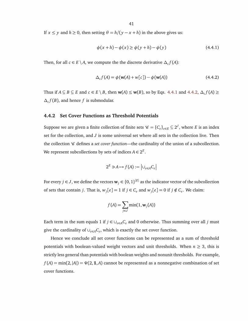
41
If x ≤ y and h≥ 0, then setting θ = h/(y − x + h) in the above gives us:
φ(x + h)−φ(x)≥ φ(y + h)−φ(y) (4.4.1)
Then, for all c ∈ E \ A, we compute the the discrete derivative ∆c f (A):
∆c f (A) = φ(w(A) +w[c])−φ(w(A)) (4.4.2)
Thus if A⊆ B ⊆ E and c ∈ E \ B, then w(A) ≤ w(B), so by Eqs. 4.4.1 and 4.4.2, ∆c f (A) ≥
∆c f (B), and hence f is submodular.
4.4.2 Set Cover Functions as Threshold Potentials
Suppose we are given a finite collection of finite sets C = Cee∈E ⊆ 2J , where E is an index
set for the collection, and J is some universal set where all sets in the collection live. Then
the collection C defines a set cover function—the cardinality of the union of a subcollection.
We represent subcollections by sets of indices A∈ 2E .
2E 3 A 7→ f (A) :=
∪e∈ACe
For every j ∈ J , we define the vectors w j ∈ 0, 1|E| as the indicator vector of the subcollection
of sets that contain j. That is, w j[e] = 1 if j ∈ Ce and w j[e] = 0 if j /∈ Ce. We claim:
f (A) =∑
j∈J
min(1,w j(A))
Each term in the sum equals 1 if j ∈ ∪e∈ACe and 0 otherwise. Thus summing over all j must
give the cardinality of ∪e∈ACe, which is exactly the set cover function.
Hence we conclude all set cover functions can be represented as a sum of threshold
potentials with boolean-valued weight vectors and unit thresholds. When n ≥ 3, this is
strictly less general than potentials with boolean weights and nonunit thresholds. For example,
f (A) =min(2, |A|) = Ψ(2,1, A) cannot be represented as a nonnegative combination of set
cover functions.

42
4.4.3 Reformulation of a Class of Functions
Another example of decomposable functions are the problems under consideration in [II07],
which are of the following form:
f (A) = u(A)φ(v(A))
Where u,v are nonnegative weight vectors and φ is a nonincreasing concave function.
Suppose we can construct a vector we for each e ∈ E and a concave function φ0 such that
the following holds for all A∈ 2E:
φ0(we(A)) =
φ(v(A))−φ(0) if e ∈ A
0 if e ∈ E \ A(4.4.3)
Then we claim the following is an equivalent formulation for f in decomposable form:
g(A) = ⟨1A,φ(0)u⟩+∑
e∈E
u[e]φ0(we(A)) (4.4.4)
Indeed, plugging Equation 4.4.3 to the above gives:
g(A) = ⟨1A,φ(0)u⟩+∑
e∈A
u[e](φ(v(A))−φ(0)) = f (A)
To satisfy Equation 4.4.3 we define φ0 as follows:
φ0(t) =
0 if t ≤ v(E)
φ(t − v(E))−φ(0) if t > v(E)
And let we = v+ v(E) 1e. It is straightforward to check that these definitions satisfy Equa-
tion 4.4.3. Note φ0 is concave because φ is nonincreasing concave. Incidentally, the decom-
position in Equation 4.4.4 proves that f is submodular.

43
4.4.4 Strict Generality of Threshold Potentials
Any concave cardinality function can be decomposed into the sum of several threshold
potentials with Boolean weight vectors. Equivalently, it is representable as a nonnegative
combination of set cover functions.
φ(|A∩ B|) = φ(0) + (φ(|B|)−φ(|B| − 1))⟨1A,1B⟩
+|B|−1∑
k=1
(2φ(k)−φ(k− 1)−φ(k+ 1))min(k, ⟨1A,1B⟩)
Since φ is concave, the coefficients (2φ(k)−φ(k− 1)−φ(k+ 1)) are positive. So without
loss of generality, any sum of concave cardinality functions can be expressed as a sum of a
modular function and a positive combination of threshold potentials with Boolean weights.
f (A) = p0 + p1(A) +∑
B∈2E
|B|≥2
|B|−1∑
k=1
r(B, k)min(k, ⟨1A,1B⟩) (4.4.5)
There are∑n
k=2
nk
(k−1) = 1+2n−1(n−2) coefficients r(B, k) and they all must be nonneg-
ative. If n is small enough, we can evaluate all 2n values of a set function and use a linear
program solver to find a representation of the above form, if one exists. When n= 4, this
is an LP feasibility problem with 5 unconstrained variables (the offset p0 and the modular
part p1), 17 nonnegative variables (the coefficients r(B, k)), and 16 equality constraints
(the values of f ). We discovered that the threshold potential f (A) = min(τ,w(A)) with
w= [1/2, 1/2, 1/2, 1] and τ= 1 does not have a feasible solution to Equation 4.4.5.
Note that any decomposable function can be represented as a finite sum of threshold
potentials. This is because w(A) can only equal finitely many values, and for any concave
function, we can construct a positive combination of threshold potentials that agrees with
the concave function on those values. For any one-dimensional function φ and any finite set
of arguments z1 < . . .< zm, define the piecewise linear interpolant φ:
φ(z) = p0 + p1z +m−1∑
i=2
ri min(z, zi) (4.4.6)
p0 = φ(z1)− z1φ(z2)−φ(z1)
z2 − z1

44
p1 =φ(zm)−φ(zm−1)
zm − zm−1
ri =φ(zi)−φ(zi−1)
zi − zi−1−φ(zi+1)−φ(zi)
zi+1 − zifor i = 2 . . . m− 1 (4.4.7)
It is straightforward to check that φ(zi) = φ(zi) for all zi, which justifies our claim that φ is
an interpolant for φ. By construction in Equation 4.4.6, φ(z) is a linear function plus a linear
combination of threshold functions. The coefficients ri in Equation 4.4.7 are positive for all
choices of zi if and only if φ is concave. Hence to represent a general concave potential as
a sum of threshold potentials, we take zimi=1 = w(A) | A∈ 2E , where m is the number
of possible values of w(A). Thus φ(w(A)) = φ(w(A)) for all A ∈ 2E . However, for general
weight vectors, m could equal 2n. This means that to use the formula in Equation 4.4.6,
we need exponentially many threshold potentials to represent the function φ(w(A)) exactly.
So even though general concave functions do not induce a strictly more general class of
submodular functions, they can provide a much more compact representation for functions
in this class.
4.5 The SLG Algorithm for Threshold Potentials
We now present our algorithm for efficient minimization of a decomposable submodular
function f based on smoothed convex minimization. We first show how we can efficiently
smooth the Lovász extension of f . We then apply accelerated gradient descent to the gradient
of the smoothed function. Lastly, we demonstrate how we can often obtain a certificate of
optimality that allows us to stop early, drastically speeding up the algorithm in practice.
4.5.1 The Smoothed Extension of a Threshold Potential
The key challenge in our algorithm is to efficiently smooth the Lovász extension of f , so that
we can resort to algorithms for accelerated convex minimization. We now show how we can
efficiently smooth the threshold potentials Ψ(τ,w, A) =min(τ,w(A)) of Section 4.3, which
are simple enough to allow efficient smoothing, but rich enough when combined to express
a large class of submodular functions. We denote the base polytope of a single threshold

45
potential Ψ(τ,w, ·) by BΨ(τ,w,·) =B(τ,w). The Lovász extension of Ψ(τ,w, ·) is thus:
Ψ(τ,w,x) = maxλ∈B(τ,w)
⟨x,λ⟩ (4.5.1)
B(τ,w) := λ ∈ Rn | ⟨1,λ⟩= τ, 0≤ λ≤w
We define a smoothed Lovász extension by taking the infimal convolution with the quadratic
function 12µ‖x‖2, where µ is a scale parameter.
Ψµ(τ,w,x) := Ψ(τ,w,x)1
2µ‖x‖2
= minz∈RnΨ(τ,w,z− x) +
1
2µ‖z‖2
= maxλ∈B(τ,w)
⟨x,λ⟩ −µ
2‖λ‖2 (4.5.2)
To give a simple justification for this definition, we note that for small µ, this function
approximates the nonsmooth function uniformly in x. We can take an optimal solution to
Equation 4.5.1 and use it in Equation 4.5.2 to get the following bound:
0≤ Ψ(τ,w,x)− Ψµ(τ,w,x)≤ µτ/2 for all x ∈ Rn
Here we use the fact that ‖λ‖2 ≤ ‖λ‖1‖λ‖∞ ≤ τ for all λ ∈ B(τ,w), since we assumed
‖w‖∞ = 1. We conclude that the smoothed extension converges uniformly to the nonsmooth
as µ→ 0.
To compute this function, we note Equation 4.5.2 is equivalent to the projection of x/µ
ontoB(w, y). Due to the simple structure of the base polytope, this can be solved efficiently.
The optimal base λ∗ is also the gradient of the smoothed extension:
∇Ψµ(τ,w,x) = arg maxλ∈B(τ,w)
⟨x,λ⟩ −µ
2‖λ‖2 = ΠB(τ,w)(x/µ). (4.5.3)
Recall that ΠC(x) := arg minx′∈C ‖x− x′‖ denotes the projection of x onto the convex set C .
To solve for λ∗, we form the Lagrangian and derive the dual problem:
Ψµ(τ,w,x) = mins∈R,y1,y2≥0
maxλ∈Rn⟨x,λ⟩ −
µ
2‖λ‖2 + ⟨y1,λ⟩+ ⟨y2,w−λ⟩+ s(τ− ⟨1,λ⟩)

46
= mint∈R,y1,y2≥0
1
2µ‖x− s1+ y1 − y2‖2 + ⟨y2,w⟩+ sτ.
In the second step the optimal λ = 1µ(x− s1+ y1 − y2). By strong duality, if the variables
s,y1,y2 are optimal for the dual problem, then λ must also be optimal. If we fix s, then we
can solve for the optimal variables y∗1 and y∗2 componentwise. So we have:
y∗1 =max(0,−x+ s∗1)
y∗2 =max(0,x− s∗1−µw)
⇒ λ∗ =max(0,min(w, (x− s∗1)/µ)). (4.5.4)
This expresses λ∗ as a function of the unknown optimal variable s∗. For the simple case of
2-potentials, we can solve for s∗ explicitly and get a closed form expression for the gradient
of the smoothed Lovász extension:
∇Ψµ(1,1bc,x) =
1b if x[b]≥ x[c] +µ
1c if x[c]≥ x[b] +µ
12(1bc +
1µ(x[b]− x[c])(1b − 1c)) if |x[b]− x[c]|< µ
For higher dimensions, it is easier to compute s∗ implicitly from the constraint ⟨1,λ∗⟩ = τ. We
defineρµx,w(s) to be the value of ⟨1,λ(s)⟩, whereλ(s) is given by the formula of Equation 4.5.4.
ρµx,w(s) :=∑
e∈E
max(0,min(w[e], (x[e]− s)/µ))
This function is a monotonic continuous piecewise linear function of s, so one approach is to
use a simple root-finding algorithm to solve ρµx,w(s∗) = τ. Additionally, in Section 5.4, we
outline two algorithms for solving this problem. First, we derive an explicit formula that
requires sorting 2n elements to compute. Also, we show how it is possible to find s∗ with a
linear number of operations (in expectation) via a randomized algorithm.
4.5.2 The SLG Algorithm for Minimizing Sums of Threshold Potentials
Stepping beyond a single threshold potential, we now assume that the submodular function
to be minimized can be written as a nonnegative linear combination of threshold potentials

47
and a modular function, i.e.,
f (A) = c(A) +∑
j
r jΨ(τ j,w j, A). (4.5.5)
So the smoothed Lovász extension of f , and its gradient (cf. Equation 4.5.3) are given by:
f µ(x) = ⟨x,c⟩+∑
j
r jΨµ(τ j,w j,x), (4.5.6)
∇ f µ(x) = c+∑
j
r jΠB(τ j ,w j)(x/µ)
We can use the accelerated gradient descent algorithm of [Nes05] to minimize this function.
This algorithm requires that the smoothed objective have a Lipschitz continuous gradient.
That is, for some constant L, it must hold that ‖∇ f µ(x)−∇ f µ(y)‖ ≤ L‖x−y‖, for all x,y ∈ Rn.
Fortunately, by construction, the smoothed threshold extensions Ψµ(τ j,w j,x) all have 1/µ
Lipschitz gradient, a direct consequence of the characterization in Equation 4.5.3. Hence
we have a loose upper bound for the Lipschitz constant of f µ: L ≤ Dµ
, where D =∑
j r j.
Furthermore, the smoothed threshold extensions approximate the threshold extensions
uniformly: |Ψµ(τ j,w j,x) − Ψ(τ j,w j,x)| ≤µτ j
2for all x, so | f µ(x) − f (x)| ≤ µD2
2, where
D2 =∑
j r jτ j.
One way to use the smoothed gradient is to specify an accuracy ε, then minimize f µ for
sufficiently small µ to guarantee that the solution will also be an approximate minimizer of
f . Then we simply apply the accelerated gradient descent algorithm of [Nes05]. See also
[BBC11] for a description. Note that the projection onto the unit cube is trivial: Π[0,1]n(x) =
max(0, min(1,x)). Algorithm 4.1 formalizes our Smoothed Lovász Gradient (SLG) algorithm.
The optimality gap of a smooth convex function at the iterate yt can be computed from its
gradient:
gapk = − minx∈[0,1]n
⟨x− yk,∇ f µ(yk)⟩= ⟨yk,∇ f µ(yk)⟩+ ⟨1, max(0,−∇ f µ(yk))⟩.
In summary, as a consequence of the results of [Nes05], we have the following guarantee
about SLG:
Theorem 4.1. SLG is guaranteed to provide an ε-optimal solution after running for O (Dε)

48
Algorithm 4.1: SLG: Smoothed Lovász GradientInput: Accuracy ε; decomposable function f .beginµ= ε
2D2, L = D
µ, x0 = z0 = 1
21;
for k = 1, 2, . . . dogk←∇ f µ(xk−1)/L;yk← Π[0,1]n(xk−1 − gk);
zk← Π[0,1]n
z0 − 12
∑kj=1 j g j
;
if gapk ≤ ε/2 then stop;;xk← (k yk + 2zk)/(k+ 2);
xε ← yk;Output: ε-optimal xε to minx∈[0,1]n f (x)
iterations.
SLG is only guaranteed to provide an ε-optimal solution to the continuous optimization
problem. Fortunately, once we have an ε-optimal point for the Lovász extension, we can
efficiently round it to set which is ε-optimal for the original submodular function using
Algorithm 4.2. As shown in Equation 4.2.3, the extension f is a convex combination of the
values of the set function, so it cannot be smaller than the smallest of those values.
Algorithm 4.2: Set Generation by Rounding the Continuous SolutionInput: Vector x ∈ [0, 1]n; submodular function f .begin
By sorting, find any permutation π satisfying: x[π1]≥ . . .≥ x[πn];$k← π1, . . . ,πk;K∗← arg mink∈0,1,...,n f ($k);C ← $k | k ∈ K∗ ;
Output: Collection of sets C , such that f (A)≤ f (x) for all A∈ C
4.5.3 Early Stopping based on Discrete Certificates of Optimality
In general, if the minimum of f is not unique, the output of SLG may be in the interior of
the unit cube. However, if f admits a unique minimum A∗, then the iterates will tend toward
the corner eA∗ . Of course, since we are actually interested in solving a discrete problem, it is
not necessary to wait for the iterates to converge to the optimal corner. Below, we show that

49
it is possible to use information about the current iterates to check optimality of a set and
terminate the algorithm before the continuous problem has converged.
To prove optimality of a candidate set A, we can use a subgradient of f at eA, which is
also a discrete subgradient for f at A. If λ ∈ ∂ f (A), and then we can compute an optimality
gap:
f (A)− f ∗ ≤ maxx∈[0,1]n
⟨1A− x,λ⟩=∑
a∈A
max(0,λ[a]) +∑
b∈E\A
max(0,−λ[b]). (4.5.7)
In particular, if λ[a] ≤ 0 for a ∈ A and λ[b] ≥ 0 for b ∈ E \ A, then A is optimal. With
only knowledge of candidate set A, finding a subgradient λ ∈ ∂ f (A) which demonstrates
optimality may be extremely difficult, as the subdifferential is a polyhedron with exponentially
many extreme points. But our algorithm naturally suggests the subgradient we could use; the
gradient of the smoothed extension is also a discrete sugradient—provided that a particular
condition holds, as described in the following Lemma.
Lemma 4.2. Suppose f is a decomposable submodular function with Lovász smoothed extension
f µ as in Equation 4.5.5 and Equation 4.5.6, respectively. If x ∈ Rn and A∈ 2E satisfy
mina∈A
x[a]≥ µ+ maxb∈E\A
x[b], (4.5.8)
then ∇ f µ(x) ∈ ∂ f (A).
Proof. By linearity of subdifferentials, it is sufficient to consider the case where f is single
threshold potential. Recall the formula for the gradient:
λ=∇Ψµ(τ,w,x) =max(0, min(w, (x− s∗1)/µ)) s∗ chosen so that ⟨1,λ⟩= τ
There are two possibilities to consider. First, if mina∈A x[a] ≤ s∗ − µ, then Equation 4.5.8
implies for all b ∈ E \ A we have x[b]< s∗ and thus λ[k] = 0. This means that λ(E \ A) = 0
and so λ(A) = λ(E) = τ. So clearly λ is a maximing base for the set A. That is, λ ∈
arg maxλ′∈B(τ,w)⟨1A,λ′⟩= ∂Ψ(τ,w,1A) ⊆ ∂Ψ(τ,w, A).
On the other hand, if mina∈A x[a]> s∗−µ, then for all a ∈ A we have (x[a]−s∗)/µ≥ 1≥
w[a] and thus λ[a] = w[a]. Therefore we must have λ(A) =w(A), and since λ′(A)≤w(A)
for any λ′ ∈B(τ,w), again it is true that λ is a maximizing base for A.

50
Lemma 4.2 states that if the components of point x corresponding to elements of A are all
larger than all the other components by at least µ, then the gradient at x is a subgradient for
f at 1A (which by Equation 4.5.7 allows us to compute an optimality gap). In practice, this
separation of components naturally occurs as the iterates move in the direction of the point
1A, long before they ever actually reach the point 1A. But even if the components are not
separated, we can easily add a positive multiple of 1A to separate them and then compute
the gradient there to get an optimality gap. In summary, we have the following algorithm to
check the optimality of a candidate set:
Algorithm 4.3: Set Optimality CheckInput: Set A; decomposable function f ; scale µ; x ∈ Rn.beginγ= µ+maxa∈A,b∈E\A x[a]− x[b];g=∇ f µ(x+ γ1A);δ =
∑
a∈A max(0, g[a]) +∑
b∈E\A max(0,−g[b]);Output: Optimality gap δ ≥ f (A)− f ∗
Of critical importance is how to choose the candidate set A. However, by Equation 4.5.7,
for a set to be optimal, we want the components of the gradient∇ f µ(x+γ1A)[a] to be negative
for a ∈ A and positive for b ∈ E \ A. So it is natural to choose A= a ∈ E | ∇ f µ(x)[a]≤ 0 .
Thus, if adding γ1A does not change the signs of the components of the gradient, then, in fact,
we have found an optimal set. We have found this stopping criterion to be quite effective in
practice, and we use it in all of our experiments.
4.6 Extension to General Concave Potentials
To extend our algorithm to work on general concave functions, we note that an arbitrary
smooth concave function can be expressed as an integral of threshold potential functions
min(x , y). Informally, this is because d2
d y2 min(x , y) = −δ(y − x), the Dirac delta. (To
see why, note min(x , y) is a piecewise linear function with a jump of −1 in its derivative
at x = y.) So, ignoring boundary terms and integrating by parts we should expect that∫
φ′′(y)min(x , y)d y =∫
φ′(y) dd y
min(x , y)d y = −∫
φ(y)δ(y − x)d x = −φ(x). We state
this formally in the following Lemma:

51
Lemma 4.3. For φ ∈ C2([0, T]),
φ(x) = φ(0) +φ′(T )x −∫ T
0
min(x , y)φ′′(y)d y, ∀x ∈ [0, T]
Proof. This is a straightforward application of integration by parts:
∫ T
0
min(x , y)φ′′(y)d y =
∫ x
0
yφ′′(y)d y +
∫ T
xxφ′′(y)d y
= (yφ′(y)−φ(y))
x0 + xφ′(y)
Tx
= xφ′(x)−φ(x) +φ(0) + xφ′(T )− xφ′(x)
= φ(0) + xφ′(T )−φ(x).
This Lemma motivates our definition of the smoothed Lovász extension for a general sum
of concave potentials. If f is decomposable as in Equation (4.3.1), we define the smoothed
extension as:
f µ(x) := ⟨c,x⟩+∑
j
φ j(0) +φ′(T j)⟨x,w j⟩ −
∫ T j
0
Ψµ(τ,w j,x)φ′′j (τ)dτ
. (4.6.1)
Here T j := w j(E). By Lemma 4.3, as µ → ∞, we have f µ → f pointwise since Ψµ → Ψ.
We can apply SLG to f µ essentially unchanged; the conditions for optimality still hold, and
so on. Conceptually, we just use a different smoothed gradient, but calculating it is more
involved. We need to compute the integrals of the form∫ T j
0 ∇Ψµ(τ,w j,x)φ′′j (τ)dτ. Since the
components of the gradient ∇Ψµ(τ,w j,x) are each piecewise linear functions with respect
to τ, we can evaluate the integral by parts. The resulting formula only evaluates φ, but not
its derivatives.
4.6.1 Formula Derivation
Let f (A) = φ(w(A)) be a general concave potential. For ease of notation, in the following
let g(τ) =∇Ψµ(τ,w,x) be the gradient of the smoothed extension of a threshold potential.
Then by Equation 4.6.1, the gradient of smoothed extention of f is given by:
∇ f µ(x) = φ′(T )w−∫ T
0
g(τ)φ′′(τ)dτ (4.6.2)

52
Note that g is a piecewise linear function of τ. Let [τi,τi+1] with 0= τ0 ≤ . . .≤ τN = T =
w(E) be the intervals on which g is linear. Let gi := g(τi). In particular, g0 = 0 and gN =w.
Denote the derivative of g(τ) with respect to τ (wherever it exists) as g′(τ). So within the
interval (τi,τi+1) it is:
g′(τi + ε) =gi+1 − gi
τi+1 −τi= g′(τi+1 − ε) (4.6.3)
So then our smoothed gradient can be evaluated:
∇ f µ(x) = φ′(τN )w−N∑
i=1
∫ τi
τi−1
g(τ)φ′′(τ)dτ
= φ′(τN )w+N∑
i=1
g′(τ)φ(τ)− g(τ)φ′(τ)
τi
τi−1
= φ′(τN )w+N∑
i=1
g′(τi − ε)(φ(τi)−φ(τi−1))−N∑
i=1
(giφ′(τi)− gi−1φ
′(τi−1))
= φ′(τN )w+N∑
i=1
(gi − gi−1)(φ(τi)−φ(τi−1))τi −τi−1
− (gNφ′(τN )− g0φ
′(τ0))
=N∑
i=1
(gi − gi−1)(φ(τi)−φ(τi−1))τi −τi−1
Interestingly, this formula no longer requires φ to be differentiable. To compute the break-
points for τ, note that τ is itself a piecewise linear function of the parameter s, implicitly
defined by the equation: ⟨1,max(0, min(w, (x− s1)/µ))⟩ = τ. The discontinuities of the
derivative occur where x[e]− s equals 0 or µw[e]. Let si be the value of s that corresponds
to τi. For a particular value of s, we say that the component of x indexed by e is an active
component if 0 ≤ x[e]− s ≤ µw[e]. Thus the difference gi − gi−1 is nonzero only in the
active components, and there it equals (si − si−1)/µ. Let Ai be the set of active components
for τ ∈ [τi−1,τi]. Then, in that interval we have dτds= |Ai|/µ and we can simplify a part of
the above sum:gi − gi−1
τi −τi−1=1Ai(si − si−1)/µ
(si − si−1)|Ai|/µ=1Ai
|Ai|. (4.6.4)
In summary, the formulas reduce to:
P = (−x[e], e), (µw[e]− x[e], e)e∈E = (si, ai), where si ≤ si+1 (4.6.5)
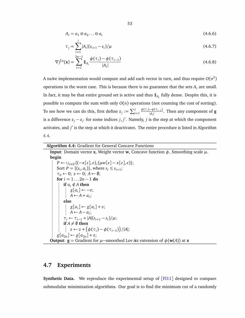
53
Ai = a1 a2 . . . ai (4.6.6)
τ j =j∑
i=1
|Ai|(si+1 − si)/µ (4.6.7)
∇ f µ(x) =2n−1∑
i=1
1Ai
φ(τi)−φ(τi−1)|Ai|
(4.6.8)
A naïve implementation would compute and add each vector in turn, and thus require O(n2)
operations in the worst case. This is because there is no guarantee that the sets Ai are small.
In fact, it may be that entire ground set is active and thus 1Aifully dense. Despite this, it is
possible to compute the sum with only O(n) operations (not counting the cost of sorting).
To see how we can do this, first define z j :=∑ j
i=1φ(τi)−φ(τi−1)
|Ai |. Then any component of g
is a difference z j − z j′ for some indices j, j′. Namely, j is the step at which the component
activates, and j′ is the step at which it deactivates. The entire procedure is listed in Algorithm
4.4.
Algorithm 4.4: Gradient for General Concave FunctionsInput: Domain vector x, Weight vector w, Concave function φ, Smoothing scale µ.begin
P ←∪e∈E(−x[e], e), (µw[e]− x[e], e);Sort P = (si, ai), where si ≤ si+1;τ0← 0; z← 0; A← ;;for i = 1 . . . 2n− 1 do
if ai /∈ A theng[ai]←−z;A← A+ ai;
elseg[ai]← g[ai] + z;A← A− ai;
τi ← τi−1 + |A|(si+1 − si)/µ;if A 6= ; then
z← z +
φ(τi)−φ(τi−1)
/|A|;g[a2n]← g[a2n] + z;
Output: g= Gradient for µ−smoothed Lovász extension of φ(w(A)) at x
4.7 Experiments
Synthetic Data. We reproduce the experimental setup of [FI11] designed to compare
submodular minimization algorithms. Our goal is to find the minimum cut of a randomly

54
R3
R1
R2
(a) Example Regions for Potentials
102
103
100
102
Problem Size (n)
Run
ning
Tim
e (s
)
SLG
SFM3
MinNorm
HYBRID
PR
LEX2
(b) Results for genrmf-long
102
103
100
102
Problem Size (n)
Run
ning
Tim
e (s
)
SLG
SFM3
MinNorm
LEX2
HYBRID
PR
(c) Results genrmf-wide
Figure 4.1: (a) Example regions used for our higher-order potential functions (b-c) Compari-sion of running times of submodular minimization algorithms on synthetic problems fromDIMACS [JM93].
generated graph (which requires submodular minimization of a sum of 2-potentials) with
the graph generated by the specifications in [JM93]. We compare against the state of the
art combinatorial algorithms (LEX2, HYBRID, SFM3, PR [FI03]) that are guaranteed to find
the exact solution in polynomial time, as well as the Minimum Norm algorithm of [FI11], a
practical alternative with unknown running time. Figures 4.1b and 4.1c compare the running
time of SLG against the running times reported in [FI11]. In some cases, SLG was 6 times
faster than the MinNorm algorithm. However, the comparison to the MinNorm algorithm
is inconclusive in this experiment, because while we used a faster machine, we also used a
simple MATLAB implementation. What is clear is that SLG scales at least as well as MinNorm
on these problems, and is practical for problem sizes that the combinatorial algorithms cannot
handle.
Image Segmentation Experiments. We also tested our algorithm on the joint image
segmentation-and-classification task introduced in Section 4.3. We used an implementation
of TextonBoost [SWRC09], then trained on and tested subsampled images from [EVGW+].
As seen in Figures 4.2e and 4.2g, using only the per-pixel score from our TextonBoost imple-
mentation gets the general area of the object, but does not do a good job of identifying the
shape of a classified object. Compare to the ground truth in Figures 4.2b and 4.2d. We then
perform MAP inference in a Markov Random Field with 2-potentials (as done in [SWRC09]).
While this regularization, as shown in Figures 4.2f and 4.2h, leads to improved performance,
it still performs poorly on classifying the boundary.
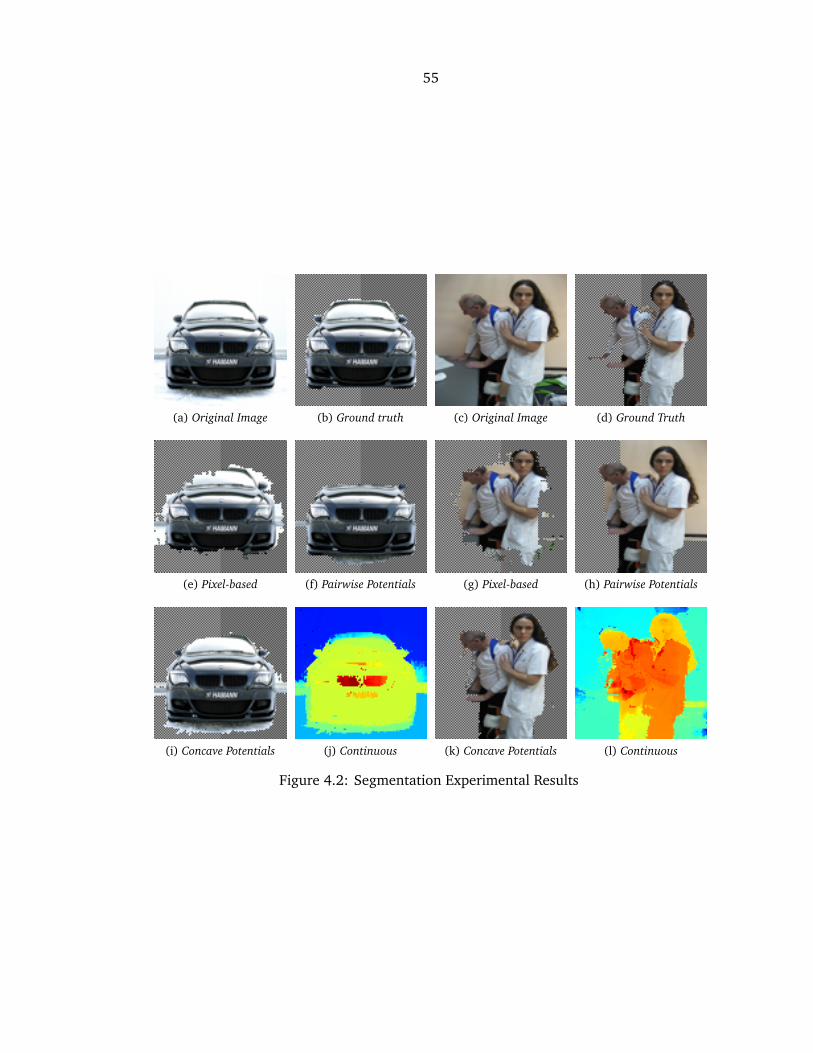
55
(a) Original Image (b) Ground truth (c) Original Image (d) Ground Truth
(e) Pixel-based (f) Pairwise Potentials (g) Pixel-based (h) Pairwise Potentials
(i) Concave Potentials (j) Continuous (k) Concave Potentials (l) Continuous
Figure 4.2: Segmentation Experimental Results

56
Finally, we used SLG to regularize with higher order potentials. To generate regions
for our potentials, we randomly picked seed pixels and grew the regions based on HSV
channels of the image. We picked our seed pixels with a preference for pixels which were
included in the least number of previously generated regions. Figure 4.1a shows what the
regions typically looked like. For our experiments, we used 90 total regions. We used SLG
to minimize f (A) = c(A) +∑
j |A∩ Dj||Dj \ A|, where c was the output from TextonBoost,
scaled appropriately. Figures 4.2i and 4.2k show the classification output. The continuous
variables x at the end of each run are shown in Figures 4.2j and 4.2l; while it has no formal
meaning, in general one can interpret a very high or low value of x[e] to correspond to high
confidence in the classification of the pixel e. To generate the result shown in Figure 4.2k, a
problem with 104 variables and 90 concave potentials, our MATLAB/mex implementation of
SLG took 71.4 seconds. In comparison, the MinNorm implementation of the SFO toolbox
[Kra10] gave the same result, but took 6900 seconds. Similar problems on an image of twice
the resolution (4× 10⁴ variables) were tested using SLG, resulting in a runtimes of roughly
1600 seconds.
4.8 Conclusion
We have developed a novel method for efficiently minimizing a large class of submodular
functions of practical importance. We do so by decomposing the function into a sum of
threshold potentials, whose Lovász extensions are convenient for using modern smoothing
techniques of convex optimization. This allows us to solve submodular minimization problems
with thousands of variables that cannot be expressed using only pairwise potentials. Thus we
have achieved a middle ground between graph-cut-based algorithms, which are extremely
fast but only able to handle very specific types of submodular minimization problems, and
combinatorial algorithms, which assume nothing but submodularity but are impractical for
large-scale problems.

57
Chapter 5
Distributed SubmodularMinimization
5.1 Introduction
Without any doubt, there have been tremendous gains in the efficiency of convex optimization
algorithms over the past century. The fact that one can now routinely solve nonlinear
constrained programs with thousands of variables is not due to advances in hardware alone.
However, there are still domains where the problem is so large that a straightforward
application of optimization algorithms is not practical. This is often due to an abundance of
data; the entire convex optimization problem cannot even be loaded in memory on a single
computer, let be alone solved in a reasonable amount of time. For such problems, the only
option is to develop algorithms that can take advantage of parallel computation. This is a
very active field of research in convex optimization. Given the strong connections between
convex and submodular minimization established in Chapter 3, a natural idea, then, is to
use techniques of distributed convex optimization for distributed submodular minimization.
First, in Section 5.2, we derive a general framework for submodular minimization using
minimization of the Lovász extension with barrier functions. This is not specific to distributed
computation, but it suggests a general technique for developing submodular minimization
algorithms. Then in Section 5.3, we use this framework by applying accelerated first-order
minimization methods to the resulting convex problems to develop submodular minimization
algorithms that can be run in parallel. Finally, in Section 5.5, we give some basic empirical
results of these algorithms on synthetic test problems.

58
5.2 Submodular Minimization with General Barrier Functions
In this section, we dissect the different ways one can formulate submodular minimization
as a convex optimization program. Let f be a submodular set function over the set E with
|E| = n. We assume f is normalized, meaning that f (;) = 0. We wish to find a minimizer of
f —any subset of E that achieves the minimal value of f :
f ∗ :=minA∈2E
f (A) (5.2.1)
Recall that a submodular function f defines a convex function over Rn called the Lovász
extension, which we denote f . It is defined as the support function of the base polytope B f .
That is: f (x) = σB f(x) =maxλ∈B f
⟨x,λ⟩. The base polytope is defined by:
B f = λ ∈ Rn | ⟨1,λ⟩= f (E), and ⟨1A,λ⟩ ≤ f (A) for all A∈ 2E .
Furthermore, minimizing the Lovász extension over the unit cube [0,1]n is equivalent to
minimizing the submodular function in the following sense: given some x∗ ∈ [0,1]n that
minimizes f and any threshold α ∈ (0, 1), the set of components of x∗ greater than or equal
to that threshold must be a minimizer of f . Note that by using an indicator function, we can
express the constrained program of minimizing over the unit cube as an unconstrained convex
program: minx f (x)+δ[0,1]n(x). In the unconstrained program, the unit cube indicator δ[0,1]n
acts as a barrier to ensure that a minimal x exists. Without it, the Lovász extension has
no finite minimizer in general. That is, unless 0 ∈ B f (or equivalently f (E) = f ∗ = 0), we
have infx∈Rn f (x) = −∞. Hence we can consider minimizing f over the unit cube to be a
particular case of a more general technique of minimizing f plus a convex barrier function
φ:
minx
f (x) +φ(x) (5.2.2)
We refer to Equation 5.2.2 as the primal program. Its corresponding dual program is:
maxλ∈B f
−φ∗(−λ) (5.2.3)
It is not immediately obvious that if we let φ be anything other than the indicator of the unit
cube that solving Equation 5.2.2 will lead to a solution of Equation 5.2.1. Indeed, we do

59
need a few conditions beyond convexity to ensure that this is the case. The first three of the
of following Properties will ensure that a minimizer of f can be computed by thresholding a
solution to the primal problem. The fourth Property is only necessary to ensure that solutions
of the dual problem will also give minimizers of f via thresholding.
Properties 5.1. Barrier Function φ with Threshold α
5.1.a The function φ is separable; it can be expressed as a sum of functions each depending
on a single coordinate. This means its conjugate φ∗ is separable as well.
5.1.b All vectors in Rn are subgradients of φ somewhere, which means φ∗ has full domain.
5.1.c At some multiple of the ones vector (α1), the only subgradient of φ is the zero vector.
This means that α1 is a strict subgradient of φ∗ at the origin.
5.1.d [Optional] The function φ is uniquely minimized at α1. This means that α1 is the
unique subgradient of φ∗ at the origin.
In summary:
φ(x) =∑
e∈E
φe(x[e]) ⇔ φ∗(λ) =∑
e∈E
φ∗e (λ[e]) (5.2.4a)
⋃
x∈dom(φ)
∂φ(x) = Rn, ⇔ dom(φ∗) = Rn (5.2.4b)
∂φ(α1) = 0 ⇔ φ∗(λ)> ⟨α1,λ⟩+φ∗(0) for all λ 6= 0 (5.2.4c)
φ(x)> φ(α1) for all x 6= α1 ⇔ ∂φ∗(0) = α1 (5.2.4d)
For example, φ(x) = δ[0,1]n(x) satisfies Properties 5.1.a through 5.1.c with any α ∈ (0, 1),
but violates Property 5.1.d. The functions φ(x) = 12‖x‖2, −
∑
e∈E log(1− x[e]2) satisfy all the
Properties with α = 0. As counterexamples, note that φ(x) = δ0(x) violates 5.1.c, whereas
φ(x)≡ 0 violates b and d, and φ(x) = ‖x‖1 violates b and c.
The purpose of Property 5.1.c is to ensure that the order of the components of the optimal
dual vector are nearly the same as the ordering of the components of the optimal primal
vector. Specifically, we will make use of the following Lemma, whose proof is obvious:
Lemma 5.1. If g is a one-dimensional convex function and ∂g(α) = β and y ∈ ∂g(x), then
y < β only if x < α, and y > β only if x > α. Conversely, we have x < α only if y ≤ β , and
x > α only if y ≥ β .

60
We will first state what we can conclude about the solutions to Equation 5.2.2 and
Equation 5.2.3 under the weaker assumption that all but the last of Properties 5.1 hold. We
state these results separately but prove them together, because the convex programs are dual
to each other.
Proposition 5.2 (Primal form). Suppose f is the Lovász extension of the submodular function
f , and φ ∈ Conv satisfies Properties 5.1.a through 5.1.c with threshold α. Let x∗ be a minimizer
of Equation 5.2.2. Define the set X++α (resp. X+α ) to be the set of components of x∗ greater than
(resp. greater than or equal to) the threshold α.
X++α := e ∈ E | x∗[e]> α
X+α := e ∈ E | x∗[e]≥ α (5.2.5)
Then X+α and X++α are minimizers of f . That is, f (X+α ) = f (X++α ) = f ∗.
Proposition 5.3 (Dual Form). Suppose φ ∈ Conv satisfies Properties 5.1.a through 5.1.c. Let
λ∗ be a maximizer of Equation 5.2.3, wherein B f is the base polytope of the submodular function
f . Define the set Λ−−0 (resp. Λ−0 ) to be the set of components of λ∗ which are negative (resp.
nonpositive).
Λ−−0 := e ∈ E | λ∗[e]< 0
Λ−0 := e ∈ E | λ∗[e]≤ 0 (5.2.6)
Then Λ−0 and Λ−−0 are respectively upper and lower bounds for minimizers of f . That is,
f (A) = f ∗, only if Λ−−0 ⊆ A⊆ Λ−0 .
Proof. Since dom f ∗ is a polyhedron and domφ∗ = Rn, we can apply Fenchel’s Duality
Theorem to the functions f and φ, which gives us:
minx∈Rn
f (x) +φ(x) =maxλ∈Rn
− f ∗(λ)−φ∗(−λ)
Since f = σB f, and f ∗ = δB f
, the right hand side is equivalent to Equation 5.2.3. By
Equation 2.1.5, the optimal solutions (x∗,λ∗) of these programs are characterized by:
λ∗ ∈ ∂ f (x∗)∩−∂φ(x∗), x∗ ∈ ∂ f ∗(λ∗)∩ ∂φ∗(−λ∗).
This implies −λ∗[e] ∈ ∂φe(x∗[e]), where φe is the one-dimensional convex function from

61
the decomposition φ(x) =∑
e∈E φe(x[e]). Thus by Lemma 5.1 and Property 5.1.c we have:
e ∈ Λ−−0 ⇔ λ∗[e]< 0 ⇒ x∗[e]> α ⇔ e ∈ X++α
e /∈ Λ−0 ⇔ λ∗[e]> 0 ⇒ x∗[e]< α ⇔ e /∈ X+α
This means that Λ−−0 ⊆ X++α ⊆ X+α ⊆ Λ−0 , hence:
λ∗[e]≥ 0 for all e ∈ X+α , λ∗[e]≤ 0 for all e ∈ E \ X++α .
Also note by Equation 3.3.9, we have λ∗ ∈ ∂ f (x∗) ⊆ ∂ f (X+α ). So the set X+α and base λ∗
satisfy the premise of Theorem 3.7, and so X+α must be a minimizer of f . Likewise, since
X++α = X+β
for some β > α, we can use Equation 3.3.9 to conclude λ∗ ∈ ∂ f (X++α ), and so by
the same argument X++α is a minimizer of f .
To prove Proposition 5.3, we use the same facts we established in the proof of Proposi-
tion 5.2. Namely, since f (X+α ) = f ∗, λ∗ ∈ ∂ f (X+α ), and Λ−−0 ⊆ X+α ⊆ Λ−0 , we can bound f (A)
for any A∈ 2E:
f (A)− f ∗ ≥ ⟨1A− 1X+α,λ∗⟩=
∑
e∈A\X+α
λ∗[e]−∑
e∈X+α \A
λ∗[e]
=∑
e∈A\Λ−0
|λ∗[e]|+∑
e∈Λ−−0 \A
|λ∗[e]|
Since |λ∗[e]| > 0 for e ∈ E \ (Λ−0 \ Λ−−0 ), if either A \ Λ−0 or Λ−−0 \ A is nonempty we have
f (A) > f ∗. Therefore, any minimizer of f must be sandwiched between Λ−−0 and Λ−0 as
claimed.
Note that if no component of λ∗ equals zero, then Λ−−0 = Λ−0 is the unique minimizer of
f . In general though, a solution to the dual problem might only give nonstrict bounds for
minimizers of f . For example, suppose E = 1,2 and f (A) = min(1, |A|). Then A∗ = ; is
the unique minimizer of f and B f = (θ , 1− θ ) | θ ∈ [0,1] . Suppose we use the barrier
function φ = δ[0,1]2 . Then φ∗(−λ) = σ[0,1]2(−λ) = 0 for all λ ∈ B f . If we take λ∗ = (1,0),
then Λ−0 = 2, which is not a minimizer of f . (This does not contradict the Theorem since
Λ−−0 = ;, hence Λ−−0 ⊆ A∗ ⊆ Λ−0 .) Likewise, it is also possible to construct an example
where Λ−−0 is not a minimizer. Consider an example identical to the previous one except
62
that f (A) = min(1, |A|) − |A|. In this case, A∗ = 1,2 is the unique minimizer of f , and
λ∗ = (−1,0) is maximal for Equation 5.2.3. But then Λ−−0 = 1 is not a minimizer of f .
Finally, note that if we take the direct product of these two examples, then we get a case
where Λ−−0 ( A∗ ( Λ−0 .
These counterexamples are due to the fact that if φ does not have a unique minimizer,
we do not have a strong enough condition on the components x∗[e] for which λ∗[e] = 0.
However, when φ is is uniquely minimized at α1, then the primal and dual problems give
identical results.
Theorem 5.4. Suppose φ ∈ Conv satisfies Properties 5.1. Let x∗ be a minimizer of Equa-
tion 5.2.2 and use it to define X++α , X+α as in Equation 5.2.5. Let λ∗ be a maximizer of Equa-
tion 5.2.3 and use it to define Λ−−0 ,Λ−0 as in in Equation 5.2.6. Then X++α = Λ−−0 is the unique
minimal minimizer of f , and X+α = Λ−0 is the unique maximal minimizer of f .
Proof. The hypothesis of the Theorem is identical to the Propositions, with the additional
assumption that Property 5.1.d holds. This extra condition implies 0 /∈ ∂φe(x) for x 6= α.
Hence:
−λ ∈ ∂φe(x)⇒
x < α ⇔ λ > 0
x = α ⇔ λ= 0
x > α ⇔ λ < 0
Thus, since −λ∗ ∈ ∂φ(x∗), we must have X++α = Λ−−0 and X+α = Λ−0 . The theorem then
follows immediately from the conclusions of Proposition 5.2 and Proposition 5.3.
Discussion The implication of this result is that we have a great deal of flexibility in how we
can solve Equation 5.2.1 through convex optimization. Any barrier function which satisfies
the conditions of the theorem can be used.
Properties 5.1 are, in some sense, necessary for the conclusions of the Theorem to hold.
Clearly B f must be contained in domφ∗, and Property 5.1.b is needed to ensure this is true
for all submodular functions f . Because Property 5.1.d is not necessary to find a minimizer
of f with the primal problem, one might suspect by symmetry that Properties 5.1.a, b and
d would be sufficient to find a minimizer of f with the dual problem. This is not the case,
however. For example, if we tried to use φ(x) = ε‖x‖1 +12‖x‖2, and B f ⊆ [−ε,ε]n, then we
63
would have x∗ = 0, and λ∗ an arbitrary point in B f , so solving this convex program would
tell us nothing useful about the the submodular minimization problem.
Note that we define the Lovász extension to be the support function of the submodular
polytope B f rather than the submodular polyhedron Pf . Using the base polytope is strictly
more general in the following sense: the Theorem still holds with Pf used in place of B f ,
provided that the threshold α > 0. To see this, first note that σPf= σB f
+ δRn+. Hence
minimizing σPf+ φ1 is equivalent to minimizing σB f
+ φ2, where φ2 = φ1 + δRn+, and
φ∗2 = φ∗1 δRn
−. Then φ2 satisfies Properties 5.1 if and only if φ1 does with α > 0.
5.3 Consensus Algorithms for Submodular Minimization
5.3.1 Notation
Using convex analysis, we can develop consensus algorithms for submodular minimization.
In particlar, suppose our submodular functions can be reprsented as a sum of a modular
function plus M submodular functions, each of which depends on a subset of the ground set.
minA
c(A) +M∑
i=1
fi(A∩ Ei)
The assumption that each subfunction fi depends only on a subset of the variables confers
no loss of generality, since we can just take each Ei to be the full ground set E if necessary.
However, it can lead to a substantially more efficient algorthm (in time and memory) in the
case where the average coverage 1M
∑Mi=1 |Ei|/|E| is small.
By Theorem 5.4, we can minimize f by computing the proximal operator of the Lovász
extension f :
minx∈Rn
1
2‖x‖2 + ⟨x,c⟩+
∑
i
fi(Pix)
Here the projection matrices Pi select out the coordinates corresponding to the sets Bi . That
is, for d ∈ Ei, e ∈ E, Pi[d, e] = [[d = e]]. Then by forming the Langragian we get the dual
problem:
maxλi
minx,xi
1
2‖x‖2 + ⟨x,c⟩+
∑
i
fi(xi) +λTi (Pix− xi)

64
maxλi
−1
2‖c+
∑
i
PTi λi‖2 −
∑
i
f ∗i (λi)
The dual functions f ∗i are indicactor functions of the corresponding base polytopes B fi. We
scale and concatenate the λi into a single vector z of size N =∑M
i=1 |Ei|
λi = SiQiz ∈ Rn
R=∑
i
PTi SiQi
The projection matrices Qi select out the appropriate coordinates of z and we choose the
scales Si so that the matrix R is a projection R2 = R. So then the problem can be written in a
form with a single vector variable:
minz∈RN
1
2‖c+Rz‖2 (5.3.1)
SiQiz ∈ B fifor i = 1. . . M
Note that any feasible z gives us a base vector for f : λ = c + Rz ∈ B f . We then apply
accelerated gradient methods to this formulation to derive algorithms. However, in the
implementations we maintain the vectors λi separately, because that is how we parallelize.
5.3.2 Outline of Algorithms
Note that Equation 5.3.1 is in a form to which we can simply apply standard first order
methods to it. We implemented and tested three different first order methods:
1. Proximal Gradient
2. Accelerated Proximal Gradient (FISTA)
3. Proximal Gradient with Barzilai-Borwein stepsizes
The last technique simply applies proximal gradient, but uses aggressive stepsizes. The idea is
that if Lk is an estimate of the Lipschitz constant used in the algorithm, O(1/k2) convergence
is guaranteed if we ensure that our updates satisfy:
Lk ≥‖R(zk+1 − zk)‖2
‖zk+1 − zk‖2(5.3.2)

65
Here R is the hessian of our objective function. A conservative option to guarantee con-
vergence is to backtrack whenever a constraint is violated; that is, discard the update zk+1,
increase Lk and project again. It is then difficult to achieve a balance between making sure
the stepsizes are large enough, but not to waste too many updates backtracking. Instead by
using Barzilai–Borwein stepsize, we simply set Lk+1 to be equal to quantity on the right-hand
side of this Equation 5.3.2 for step k. The overall behavior is to take large steps when the
projection is preventing progress in the objective, at the expense of ocasionally overstepping.
This results in non-montonic convergence.
Accelerating the Min-Norm Algorithm. Can we use accelerated methods even when there
is no algorithm for projection onto the submodular polytope? We outline a procedure that
has worked well in some limited experiments. The problem is to maximize −‖∑
λi‖2 subject
to λi ∈ B fi. Initially let λ
0i = λ
0i .
1. gk = −∑
i λki
2. Choose descent directions by maximizing the first order approximation of the objective
with the greedy method: yki = arg maxy∈B fi
(y− λki )
T gk.
3. Find coefficients β ki through box-constrained least squares:
minβi∈[0,1]
1
2
∑
i
βiyki + (1− βi)λ
ki
2
.
4. Update the vectors using an accelerated update rule: λk+1i = β k
i yki + (1 − β
ki )λ
ki ,
λik+1= λk+1
i + (αk−1)αk+1
(λk+1i −λk
i ), αk+1 =1+q
1+4α2k
2.
5. Repeat until convergence criterion is met.
In our experiments, we use another accelerated gradient method to find the β ki in step 3.
Unfortunately, the vectors λi actually can leave the constraint set, although this appears to
actually speed convergence.

66
5.4 Fast Proximal Threshold Potentials
The general principle of our consensus algorithms is to combine simple submodular functions
for which projection onto the base polytope is efficient in order to project onto the base
polytope of the sum. One class of functions for which projection is efficient are threshold
potentials, introduced in Section 4.3. To review, a threshold potential is a positive modular
function truncated at some treshold: f (A) =min(τ,w(A)), where w≥ 0 and 0< τ <w(E).
The base polytope for such a function is given by the intersection of a box with a plane:
B f = λ ∈ Rn | ⟨1,λ⟩= τ, 0≤ λ≤w . In this section, we outline two algorithms for the
general problem of projecting onto a box-plane intersection (not necessarily a base polytope).
The first method requires sorting the components of the vector to be projected, but is simple
to implement. Our second method is a randomized algorithm that runs in expected linear
time.
5.4.1 General Plane Intersection Projection
The following proposition will be useful for the characterization of projections onto convex
subsets of planes. It suggests a general method for computing the projection of a single plane
intersected with any convex set.
Proposition 5.5. Let C be any closed convex set in Rn, and P be the plane given by ⟨x,a⟩= b.
Then, for t ∈ R,
⟨ΠC(x+ ta),a⟩= b⇔ ΠC(x+ ta) = ΠC∩P(x) (5.4.1)
Proof. The backward direction of the proposition is obvious, since ΠC∩P(x) ∈ P. To prove
the forward direction, we use the following facts:
• If C is any convex set, then y= x−ΠC(x) implies that ΠC(x+ y) = ΠC(x).
• If P is a plane normal to the vector a, then ΠP(x+ a) = ΠP(x).
• If C1, C2 are any convex sets, then z = ΠC1(x + λ) = ΠC2
(x − λ) implies that z =
ΠC1∩C2(x). (This is a special case of Proposition 2.2.)
To prove the proposition we use λ = x+ ta−ΠC(x+ ta), and by the above facts ΠC(x+λ) =
ΠP(x−λ) = ΠC(x+ ta) = ΠC∩P(x).
67
How can we interpret the proposition? Suppose we start at a point x, move in the
direction normal to the plane for some distance, and then project onto C . If the resulting
point is on the plane, then it must be the projection of x onto the intersection of the plane
with C . Therefore to calculate the projection, it is a matter of finding this correct distance.
We conclude that if a convex set C is easy to project onto, this allows us to project almost
as easily onto C ∩ P. In some cases, this will give a closed form formula. For example, when
C itself is an intersection of planes, then this reduces to the matrix inversion problem of
underdetermined least squares. But if there is no closed form solution, then we can at least
say that the Proposition reduces the problem of a multi-dimensional optimization problem
to a 1-dimensional root finding problem. If we let ρ(t) = ⟨ΠC(x+ ta),a⟩, then we can use
any numerical root-finding method to solve ρ(t∗) = b. Of course, in order for this to work,
the projection ΠC must be computationally inexpensive to compute.
5.4.2 Box-Plane Projection Algorithms
For the particular case of Proposition 5.5 in which we are interested, the convex set C is
a box: x ∈ Rn | `≤ x≤ u . This is, of course, an extremely simple set to project onto.
Each component of a vector to be projected need only be compared to the boundaries of
the box and adjusted accordingly. That is, ΠC(x) =max(`,min(u,x)). As a consequence of
the Proposition, we can project onto a box-plane intersection easily, provided that we can
efficiently solve the following equation:
⟨max(`,min(u,x+ t∗a)),a⟩= b (5.4.2)
Once the satisfying value t∗ is known, the projected point is given by:
ΠC∩P(x) =max(`, min(u,x+ t∗a)) (5.4.3)
Though we could use a general numerical method to find the root of Equation 5.4.2, we can
do better with a routine specialized for this particular problem. In this case, the function
ρ(t) is monotonic and piecewise linear, which we can write as:
ρ(t) = −b+ ⟨a, max(`, min(u,x+ t∗a))⟩
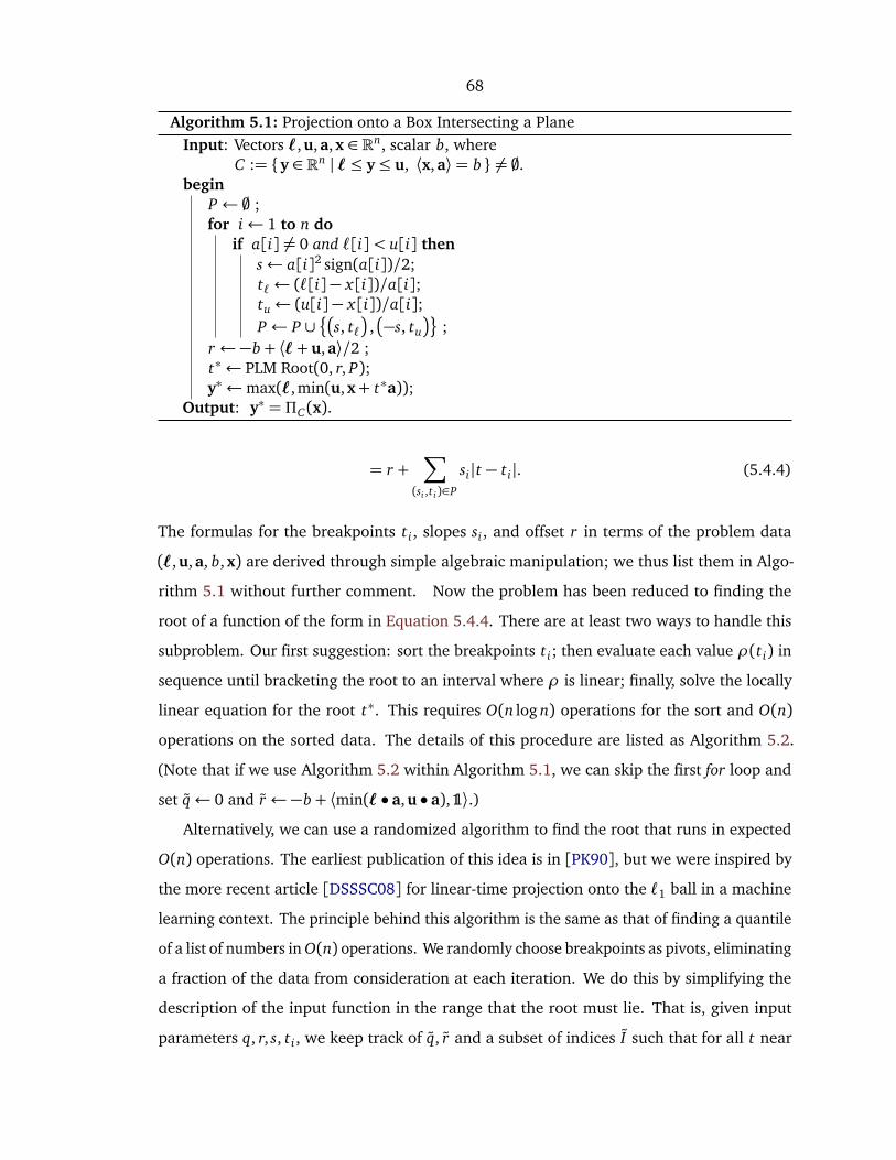
68
Algorithm 5.1: Projection onto a Box Intersecting a PlaneInput: Vectors `,u,a,x ∈ Rn, scalar b, where
C := y ∈ Rn | `≤ y≤ u, ⟨x,a⟩= b 6= ;.begin
P ← ; ;for i← 1 to n do
if a[i] 6= 0 and `[i]< u[i] thens← a[i]2 sign(a[i])/2;t`← (`[i]− x[i])/a[i];tu← (u[i]− x[i])/a[i];P ← P ∪
s, t`
,
−s, tu
;r ←−b+ ⟨`+ u,a⟩/2 ;t∗← PLM Root(0, r, P);y∗←max(`, min(u,x+ t∗a));
Output: y∗ = ΠC(x).
= r +∑
(si ,t i)∈P
si|t − t i|. (5.4.4)
The formulas for the breakpoints t i, slopes si, and offset r in terms of the problem data
(`,u,a, b,x) are derived through simple algebraic manipulation; we thus list them in Algo-
rithm 5.1 without further comment. Now the problem has been reduced to finding the
root of a function of the form in Equation 5.4.4. There are at least two ways to handle this
subproblem. Our first suggestion: sort the breakpoints t i; then evaluate each value ρ(t i) in
sequence until bracketing the root to an interval where ρ is linear; finally, solve the locally
linear equation for the root t∗. This requires O(n log n) operations for the sort and O(n)
operations on the sorted data. The details of this procedure are listed as Algorithm 5.2.
(Note that if we use Algorithm 5.2 within Algorithm 5.1, we can skip the first for loop and
set q← 0 and r ←−b+ ⟨min(` • a,u • a),1⟩.)
Alternatively, we can use a randomized algorithm to find the root that runs in expected
O(n) operations. The earliest publication of this idea is in [PK90], but we were inspired by
the more recent article [DSSSC08] for linear-time projection onto the `1 ball in a machine
learning context. The principle behind this algorithm is the same as that of finding a quantile
of a list of numbers in O(n) operations. We randomly choose breakpoints as pivots, eliminating
a fraction of the data from consideration at each iteration. We do this by simplifying the
description of the input function in the range that the root must lie. That is, given input
parameters q, r, s, t i, we keep track of q, r and a subset of indices I such that for all t near

69
Algorithm 5.2: PLM Root: Sorted Version
Input: Piecewise Linear Monotonic Function ρ(t) = qt + r +∑
i si|t − t i|, representedby: Scalars q, r, List of ordered pairs P = (si, t i)i, sorted so that t i ≤ t i+1.
beginq← q; r ← r;for i = 1 to |P| do
q← q− si ;r ← r + si t i ;
t ← 0;for i = 1 to |P| do
r ← r + q(t i − t);t ← t i;if r ≥ 0 then stop;;q← q+ 2si ;
if q 6= 0 thent ← t − r/q;
Output: t satisfying ρ(t) = 0
the root of the function we have:
qt + r +∑
i∈I
si|t − t i|= qt + r +∑
i∈ I
si|t − t i|
The details of this are shown in Algorithm 5.3.
5.5 Experiments
Since we can easily compute the proximal operator for a threshold potential, we use our
algorithms to minimize a sum of threshold potentials. We tested on a synthetic problem
designed to mimic semi-supervised learning. Given n points in some metric space, we define
weight vectors: w[ j] = w0 exp(−d(i, j)/d0)2) where d(i, j) is the distance between i and j,
and w0 and d0 are model parameters. Then given a vector of partial (possibly noisy) labels
c ∈ −1,0,+1, we minimize the following to classify the points:
f (A) = c(A) +∑
i
min(wi(A),wi(E \ A))
See Figure 5.1 for an example of a problem. Figure 5.4 and Figure 5.3 show examples of
program output using two of our techniques (FISTA and the Barzilai–Borwein proximal

70
Algorithm 5.3: PLM Root: Unsorted Version
Input: Piecewise Linear Monotonic Function ρ(t) = qt + r +∑
i si|t − t i|, representedby: Scalars q, r, Unsorted list of ordered pairs P = (si, t i)i.
beginq← q; r ← r; P ← P;while P 6= ; do
Choose (s0, t0) at random from P ;dq`← 0; dr`← 0; P`← ;;dqu← 0; dru← 0; Pu← ;;for (si, t i) ∈ P do
if t i > t0 thenPu← Pu ∪
(si, t i)
;else
dqu← dqu + si;dru← dru − si t i;
if t i < t0 thenP`← P` ∪
(si, t i)
;else
dq`← dq` − si;dr`← dr` + si t i;
v0← (q+ dqu + dq`)t0 + r + dru + dr` ;if v0 < 0 then
q← q+ dqu;r ← r + dru;P ← Pu;
else if v0 > 0 thenq← q+ dq`;r ← r + dr`;P ← P`;
elset ← t0;stop while;
if P = ; thent ←−r/q ;
Output: t satisfying ρ(t) = 0

71
Figure 5.1: Example Synthetic Semi-Supervised Learning Problem. 10000 total points. 90labeled points.
gradient). Note the nonmonotonic convergence of the latter method. In Figure 5.2, we show
the results dividing up the number of potentials across different simulated processors to
examine the effect of parallelization. Since the main bottleneck of implementation is the
computing the projections, which parallelizes perfectly across processors, we see close to
ideal speedup times.
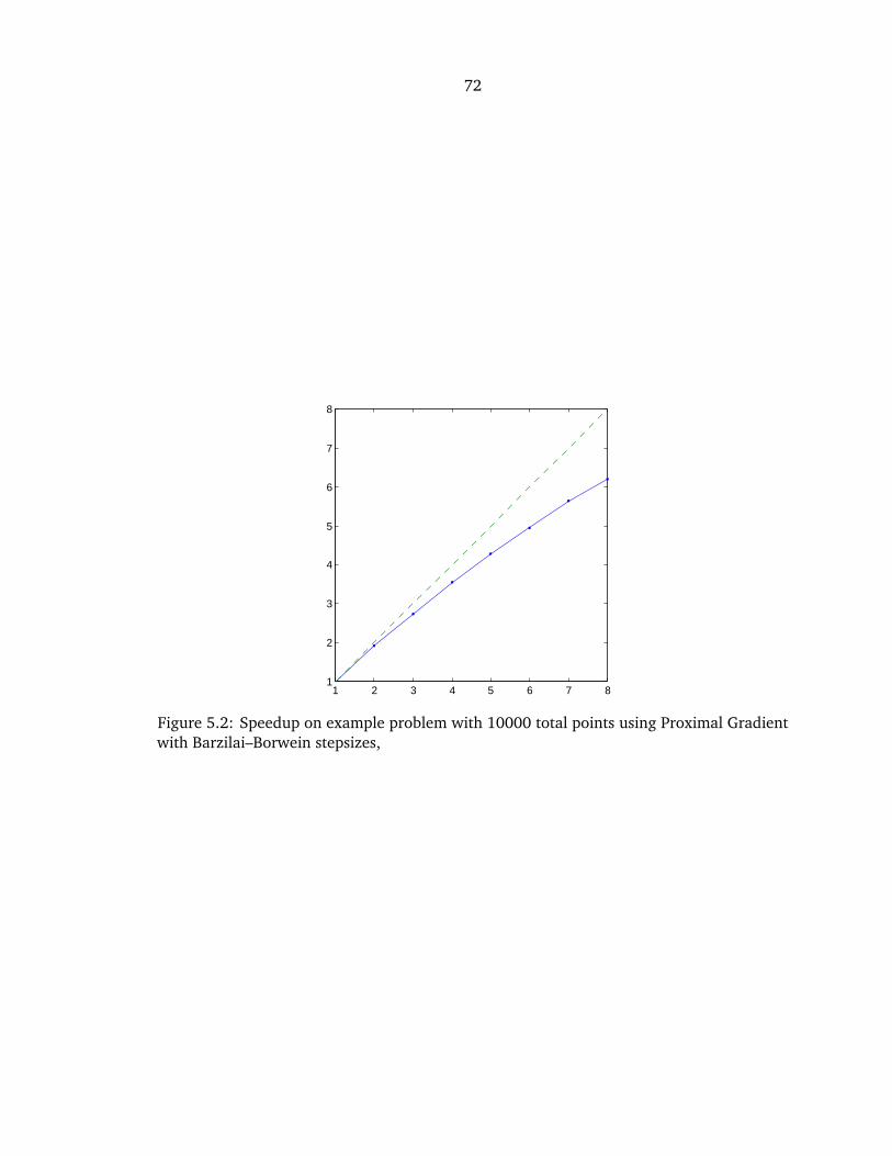
72
1 2 3 4 5 6 7 81
2
3
4
5
6
7
8
Figure 5.2: Speedup on example problem with 10000 total points using Proximal Gradientwith Barzilai–Borwein stepsizes,
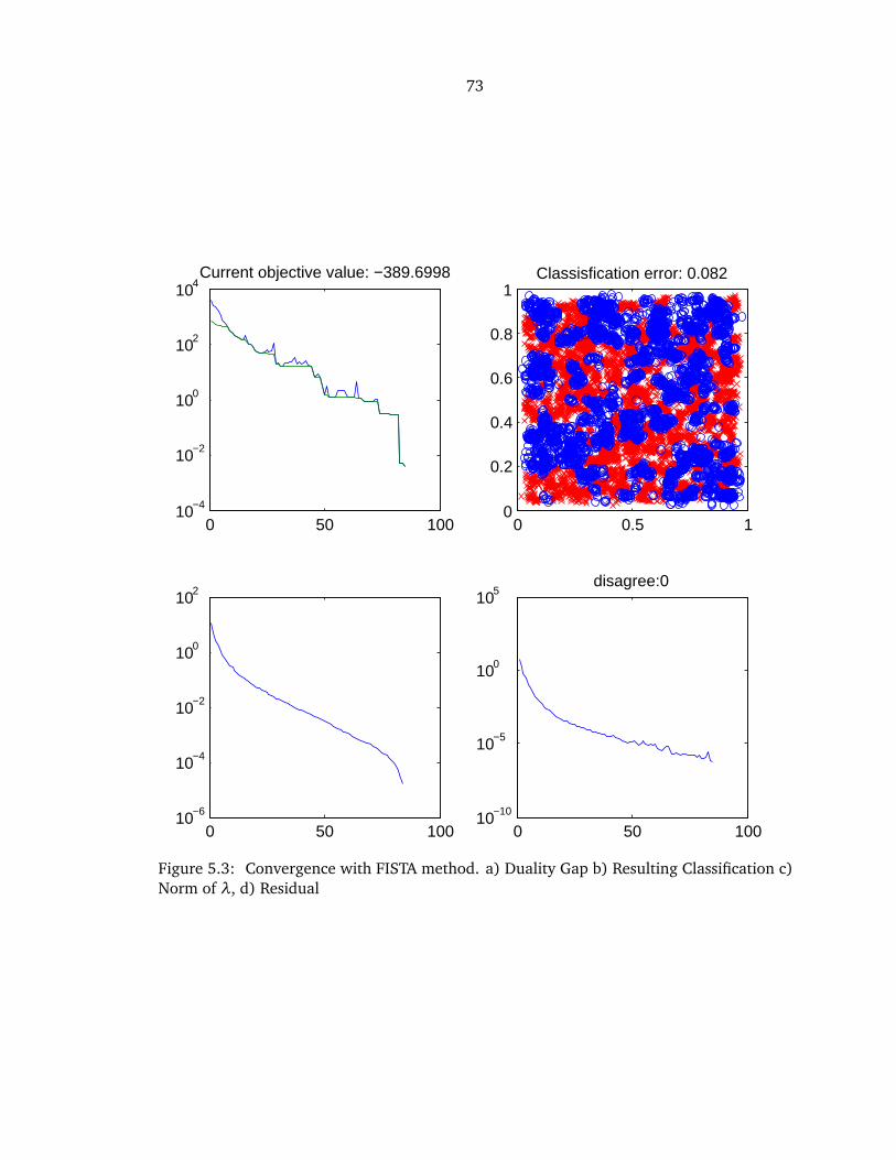
73
0 50 10010−4
10−2
100
102
104Current objective value: −389.6998
0 0.5 10
0.2
0.4
0.6
0.8
1Classisfication error: 0.082
0 50 10010−6
10−4
10−2
100
102
0 50 10010−10
10−5
100
105disagree:0
Figure 5.3: Convergence with FISTA method. a) Duality Gap b) Resulting Classification c)Norm of λ, d) Residual
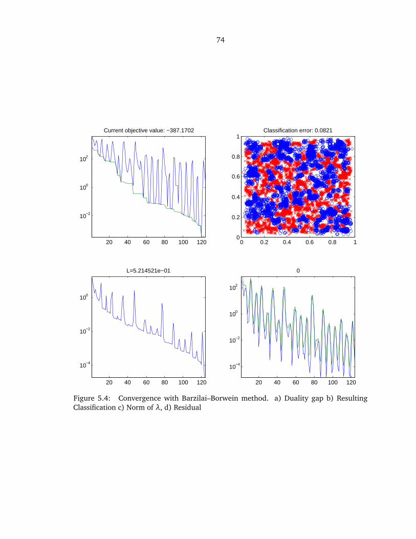
74
0 0.2 0.4 0.6 0.8 10
0.2
0.4
0.6
0.8
1Classification error: 0.0821
20 40 60 80 100 120
10−4
10−2
100
102
0
20 40 60 80 100 120
10−2
100
102
Current objective value: −387.1702
20 40 60 80 100 120
10−4
10−2
100
L=5.214521e−01
Figure 5.4: Convergence with Barzilai–Borwein method. a) Duality gap b) ResultingClassification c) Norm of λ, d) Residual

75
Chapter 6
Learning Fourier Sparse SetFunctions
6.1 Introduction
Suppose we wish to sketch the evolution of a massive network: we are given a sequence of
networks, where between each step, only few edges get added or removed. Can we compute
a small number of statistics, which allow, in hindsight, to reconstruct which edges got added
or removed, without storing the entire network? In this chapter, we show that this is possible
by observing and storing a small number of random cuts and their values.
Formally, we consider the problem of learning a set function f (mapping subsets of some
finite set E of size n to the real numbers) by observing its value on a few sets. Without
observing any structure, we clearly need an exponential (in n) number of observations to
approximate the function well over all sets, so we need an appropriate regularity condition.
To that end, we consider the situation where f is smooth in the sense of having a decaying
Fourier (Hadamard-Walsh) spectrum. One natural example of this is the cut function of a
(possibly directed) graph, or generalized additively independent (GAI) functions [Fis67],
that decompose into a sum of local terms.
By leveraging recent results from sparse recovery [Ver12], we show that if the function is
sparse in the Fourier domain, having at most k nonzero coefficients, and support contained
in a known collection P of size p, then it is possible to efficiently recover the function exactly
from very few samples. In particular, suppose we pick O(k log4
p
) sets uniformly at random.
Then with very high probability (over this random choice), observing the values of the
function on these sets is sufficient to exactly reconstruct it.

76
Besides decaying Fourier spectrum, many set functions encountered in practice satisfy
additional properties. In particular, we consider submodular functions, which form a natural
discrete analogue of convex functions [Lov83]. Submodularity is satisfied by numerous
set functions encountered in practice, such as the cut function in graphs [Sch03], entropy
[KK80], mutual information [KSG08] etc. The problem of learning submodular functions
has received considerable attention recently [GHIM09, BH11]. However, approximating a
submodular function by a factor better thanp
n/ log n uniformly over all sets requires an
exponential number of function evaluations, even if those can be adaptively chosen [GHIM09].
We show that submodularity implies certain structure in the Fourier domain, which can be
exploited to reduce the number of required samples even further.
Besides allowing us to sketch the evolution of large graphs by observing the value of a few
random cuts, as mentioned above, our results show that practically relevant set functions, such
as certain valuation functions, a fundamental concept in economics capturing substitutability
of certain products, can be efficiently learned from few examples. Another natural application
is in speeding up submodular optimization: standard algorithms assume that the function f
is presented by an oracle, which evaluates f on any set. In general, evaluating f can be very
costly (requiring the solution of a large linear system, or perform large-scale simulations). In
such a setting, if f is Fourier-sparse, we can approximate it compactly using a small number
of random sets, and then optimize the compact representation instead.
In summary, our main contributions are:
• We show that it is possible to learn Fourier k-sparse set functions exactly using
O(k log4
p
) random samples. This reconstruction is robust to noise.
• We show that properties such as symmetry and submodularity of f imply structure
in the Fourier domain, which can be exploited to obtain further reduction in sample
complexity.
• We demonstrate our algorithm on a problem of sketching the evolution of a graph, and
on approximate submodular optimization.

77
6.2 Background
Recall that we define H = R2Eto be the space of set functions with ground set E, which
is of size n. Suppose we are given the value of a set function f ∈H on some collection of
subsets. For now, let us assume that these observations are noise free – we will relax this
condition later. Under what conditions can we hope to recover f ? Clearly, without any
assumptions about f , we need an exponential number (in n) of samples in order to obtain
exact reconstruction. However, if f is smooth in some way, we may hope to do better. Similar
to continuous functions, a natural smoothness condition is decaying Fourier spectrum.
6.2.1 The Fourier transform on set functions.
Set functions can equivalently be represented as real-valued functions of boolean vectors,
known as pseudoboolean functions. Just as the set of boolean vectors 0,1n forms the
commutative group Zn2 under addition modulo 2, the power set 2E forms an equivalent group
under the operation of symmetric set difference: A B := (A\ B)∪ (B \ A). So the space H
has a natural Fourier (also called Hadamard-Walsh) basis, and in our set function notation
the corresponding Fourier basis vectors, or Fourier modes, are defined as:
ψB(A) := (−1)|A∩B|.
The space H is endowed with the standard inner product: ⟨ f , g⟩ := 2−n∑
A∈2E f (A)g(A). The
Fourier transform of a function is given by its inner products with Fourier modes:
bf (B) := ⟨ f ,ψB⟩= 2−n∑
A∈2E
f (A)(−1)|A∩B|.
Note that the sum in this definition has exponentially many terms, so it is not practical
to evaluate directly. As with any orthonormal basis, we have a reconstruction formula:
f (A) =∑
B∈2E bf (B)ψB(A).
The Fourier support of a set function is the collection of subsets with nonzero Fourier
coefficient: Supp[bf ] := B ∈ 2E | bf (B) 6= 0 . Given a collection of subsets P ⊆ 2E , let
HP := f ∈H | Supp[bf ] ⊆ P be the subspace with Fourier support contained in P. We
assume we have some a priori knowledge about the Fourier support which gives a natural

78
choice for P. We discuss this in further detail in Section 6.4, but for now assume P is some
known collection of polynomial size. One illustrative example is the collection of sets of size
q or less: Pq := B ∈ 2E | |B| ≤ q . As it is particularly important, we denote this function
space, consisting of all functions of order q or less, by the symbol Hq. The number of free
parameters is p =∑q
j=0
nj
, which is not too large when q = 2.
Now with P fixed, suppose we restrict ourselves to f ∈ HP. Can we recover f with a
subexponential number of samples? In the next section, we show that if the Fourier support
is small, then this is indeed possible by leveraging recent results from sparse reconstruction.
6.3 Conditions for Recovery
Since a set function is uniquely determined by its Fourier transform, recovering a Fourier-
sparse function can be thought of as recovery of a sparse vector in R2n. For large n, even
representing such vectors will be intractable. However, if we know that the Fourier support
of a function is contained in P, then, instead, we treat bf as a sparse vector in Rp. We will
show that it is possible to uniquely recover any f ∈HP with |Supp[bf ]| ≤ k by observing the
values fM (with high probability over the choice of measurement sets M), provided that
m= O(k log4(p)).
Matrix vector notation. In the problems that we consider, we observe the function f
evaluated on sets from a measurement collection M = Ai of size m. We arrange these
measurements in a vector fM ∈ Rm, where fM[i] := f (Ai) for i = 1 . . . m. Note the bold
typeface used to distinguish vectors from set functions. Furthermore, we will assume that the
Fourier support is contained in a known potential support collection P= B j of size p. We
denote fP ∈ Rp for the the corresponding vector of Fourier coefficients, where fP[ j] := bf (B j)
for j = 1 . . . p. Lastly, we denote ΨM,P for the m× p matrix which relates the two vectors,
ΨM,P[i, j] :=ψB j(Ai) = (−1)|Ai∩B j |. (6.3.1)
Then for f ∈HP we have:
fM =ΨM,P fP. (6.3.2)

79
So recovery of f is equivalent to recovery of a sparse vector from linear measurements.
Restricted Isometry. The problem of finding a k-sparse vector from an underdetermined
linear system has received significant attention in the context of compressive sensing [CRT06,
Don06]. A sufficient condition for recovery is that the sensing matrix satisfies a key property,
the Restricted Isometry Property (RIP). In order to ensure that our measurement matrix ΨM,P
satisfies this property, we simply choose the measurement sets M= A1, . . . , Am uniformly
at random. Then, as we will see below, results in random matrix theory imply that with
high probability (for any fixed P), the measurement matrix indeed satisfies RIP. This insight
opens up a vast collection of tools from compressive sensing for the purpose of recovering
set functions.
The idea behind RIP is that a matrix acts approximately as an isometry on sparse vectors.
Specifically, suppose for some sparsity level k and δ ≥ 0 we have:
(1−δ)‖x‖2 ≤ ‖Φx‖2 ≤ (1+δ)‖x‖2 for all x ∈ Rp with Supp[x]≤ k (6.3.3)
We define δk(Φ) as the smallest value of δ such that Equation 6.3.3 holds. An easy conse-
quence of this definition is that the linear measurement vector y = Φx0 uniquely determines
any k-sparse x0 if and only if δ2k < 1. Furthermore, with a stronger assumption on the
isometry constants, the original vector can be recovered by solving a convex optimization
problem:
minx∈Rp
‖x‖1, Φx= y (6.3.4)
Originally, [CT05] showed that Equation 6.3.4 recovers any k-sparse x0 if δ3k + 3δ4k < 2,
but this condition has been weakened several times, most recently in [Fou10], which gives
the condition δ2k (Φ)< 3/(4+p
6)≈ .465. Furthermore, as discussed below, this result can
be generalized to noisy measurements.
Main Reconstruction Result As discussed above, RIP is a very powerful property, but it is
not easy to check that any given matrix satisifies it. In fact, most constructions are based
on choosing measurements with randomness and then calculating the likelihood of RIP.
Perhaps the simplest such case is for random matrices with independent subgaussian entries.
However, in our case, we are randomly sampling rows from an orthonormal matrix with

80
bounded entries. Fortunately, as shown Rudelson and Vershynin [RV08] [Ver12], even in this
setting, as long as m= O(k log4(p)), the expectation of the kth RIP constant is small. More
recently, [Rau10] demonstrated that RIP for such matrices holds with high probability. Our
result below is essentially Theorem 4.4 of [Rau10] as applied to our case of set functions.
Theorem 6.1. For a fixed collection P = B jpj=1 ⊂ 2E , suppose a measurement collection
M = Aimi=1 ⊂ 2E is chosen by selecting the sets Ai uniformly at random. Define the matrix
ΨM,P ∈ Rm×p as in Equation 6.3.1. Then there exist universal constants C1, C2 > 0 such that if
k ≤ p/2, and m≥max(C1k log4(p), C2k log(1/δ)), except for an event of probability no more
than δ, the following holds for all f ∈HP:
For any noise level η≥ 0 and any noisy vector of measurements y ∈ Rm within that noise
level: ‖y − fM‖2 ≤ η, suppose g ∈HP has Fourier transform vector gP ∈ Rp given by :
gP = arg minx∈Rp
‖x‖1, ‖y−ΨM,Px‖2 ≤ η. (6.3.5)
Then the following bound holds for some universal constants C3, C4:
‖ f − g‖2 ≤C3p
kµk (f) +
C4pmη, (6.3.6)
where the quantity µk(·) is defined as the `1 error of the best k-sparse approximation.
µk(x) := minSupp(z)≤k
‖x− z‖1 (6.3.7)
In particular, if fP is k-sparse and η= 0, then g = f .
Therefore, we obtain a strong guarantee for efficiently (using convex optimization)
learning Fourier-sparse set functions, robust against measurement noise. Note that, up to
log factors, this matches lower bounds of [CJK11], who show that Ω(k log n) measurements
are necessary for recovery of a k sparse function in Hq with q fixed.
6.4 Classes of Set Functions
In general, p is superlinear in n, so even though Equation 6.3.4 is equivalent to a Linear
Program, it will not necessarily lead to an efficient recovery algorithm. In the extreme case,

81
if P= 2E , then even calculating a single matrix-vector product ΨTM,Py is difficult. So even
though the recovery guarantees of Theorem 6.1 apply to arbitrary collections P, we need to
make some further assumptions about our function to get a practical algorithm for recovery.
6.4.1 Symmetric functions.
One natural structural property, obeyed by set functions commonly arising in practice, is
symmetry. That is, for all sets A it holds that f (A) = f (E \A). Examples of functions satisfying
this property are the cut function in undirected graphs, as well as the mutual information,
both considered in our experiments (cf. Section 6.6). It turns out that symmetry already
implies interesting structure in the Fourier domain:
Proposition 6.2. Let f be a symmetric set function. Then for all sets B of odd cardinality, it
holds that bf (B) = 0.
Therefore, symmetry already implies that we can restrict P only to sets of odd cardinality.
6.4.2 Low order functions.
In 3.2.2, we defined the subspace Hq of order q functions. The following characterizations
are all equivalent:
Properties 6.1. Low Order Characterizations
1. ∆B f (A) = 0 for all A, B ∈ 2E with |B|> q.
2. bf (B) = 0 for all B ∈ 2E with |B|> q.
3. f (A) =∑
B [[B ⊆ A, |B| ≤ q]]∆B f (;) for all A∈ 2E .
4.∑
J⊆0,1...q+10∈J
(−1)|J | f
i∈JAi
= 0, for all A0, A1 . . . Aq+1 ∈ 2E .
5. There exist gi ∈H and |Bi| ≤ q such that f (A) =∑
i gi(A∩ Bi) for all A∈ 2E .
Many set functions f are low-order, or well-approximated by a low-order function.
Recovery of an order 1 function is equivalent to classical compressed sensing with a Bernoulli
measurement matrix (assuming we ignore the constant offset f (;)). Recovery of a symmetric
order 2 function can be thought of as recovering a graph from values of a cut function,
a problem which received considerable interest, partly due to several problems arising in

82
computational biology [ABK+04, GK00, CK10]. We can see the correspondence as follows:
given a weighted undirected graph, defined by a matrix of edge weights W, define the
symmetric cut function over sets of vertices of the graph:
φW (A) :=∑
u∈A,v /∈A
W [u, v]. (6.4.1)
Then the Fourier transform can be computed explicity:
ÒφW (B) =
12
∑
u,v W [u, v], B = ;
−12W [u, v], B = u, v
0, otherwise.
(6.4.2)
Hence there is a simple linear correspondence between weights of a graph and the 2nd order
Fourier coefficients of φW. Clearly, this correspondence works in reverse, i.e., given any
symmetric 2nd order function f , there is a unique graph such that f (A)− f (;) = φW(A). In
the general case, functions in Hq can be thought of as cut functions of hypergraphs of degree
q, as considered in [BM10].
6.4.3 Submodular functions.
Another structural property exhibited by many set functions of practical importance is
submodularity, a natural discrete analogue of convexity [Lov83]. We present a definition of
submodular functions emphasizing the Fourier transform. The shift operator and discrete
difference operator are eigenfunctions of the Fourier transform. The shift operator applied
to a Fourier mode is SBψC(A) =ψC(B)ψC(A), and the discrete difference of a Fourier mode
is ∆BψC(A) = [[B ⊆ C]] (−2)|B|ψC(A). Submodular functions are those with nonnegative
second order differences: ∆B f (A)≤ 0 where A and B are disjoint, and B is a set of size two.
We can drop the restriction that A and B are disjoint by multiplying by the corresponding
Fourier mode, giving us following characterization of the cone of submodular functions:
H−2 = f ∈H |ψB(A)∆B f (A)≤ 0 for all A, B ∈ 2E , |B|= 2 .

83
While submodularity does not immediately restrict the set P of candidate supports, it immedi-
ately implies dependence among the Fourier coefficients, (a subset of) which can be encoded
as constraints in the convex program solved during recovery. In particular, submodularity
can be characterized in the Fourier domain. By using Equation 3.2.5 to express a second
order difference as a sum of Fourier coefficient, we see that f is submodular if and only if for
all |B|= 2 and A⊆ E \ B:
bf (B) +∑
C∈2E
[[B ( C]] bf (C)ψC(A)≤ 0 (6.4.3)
Checking submodularity is no easier in the Fourier domain; it still requires checking at least
2n−2n
2
inequalities. However, we can get a necessary condition for submodularity.
Proposition 6.3. For all f ∈H−2 , and |B|= 2, B ( C,
bf (B) + |bf (C)| ≤ 0. (6.4.4)
Proof. Given a particular C1 such that B ( C1, let Q := A∈ 2E |ψC1(A) = sign(bf (C1)) . By
summing Equation 6.4.3 over all A∈Q, we have:
∑
A∈Q
bf (B) +∑
C∈2E
[[B ( C]] bf (C)ψC(A)
≤ 0
|Q| bf (B) +∑
C∈2E
[[B ( C]] bf (C)∑
A∈QψC(A)≤ 0 (6.4.5)
Fix a set C2 from the inner sum of Equation 6.4.5. We claim if C1 6= C2, then there is some
set D such that A ∈ Q ⇔ A D ∈ Q, and ψC2(A) = −ψC2
(A D), so∑
A∈QψC2(A) = 0 by
symmetry. To construct a set D which will satisfy the claim, at least one of the following two
possibilities must work:
1. Choose any c ∈ C2 \ C1, and let D = c
2. Choose any b ∈ B, and c ∈ C1 \ C2, and let D = b, c
In summary, we have:
∑
A∈QψC2(A) =
0 if B ⊆ C2 and C2 6= C1
|Q| sign(bf (C1)) if C2 = C1
84
Thus Equation 6.4.5 reduces to |Q| bf (B)+ bf (C1)|Q| sign(bf (C1))≤ 0, which is then equivalent
to Equation 6.4.4 as desired.
This has an immediate simple implication about the support of a submodular function:
Corollary 6.4. For f ∈H−2 , if C ∈ Supp[bf ], then B ∈ Supp[bf ] for all B ⊂ C with |B|= 2.
Besides providing some intuition about the Fourier support of submodular functions,
Equation 6.4.4 gives a relatively simple convex constraint that can be incorporated into our
recovery program. In general, adding any valid convex constraint can never increase our
recovery error (a simple consequnce of convexity), and in practice it often decreases it.
There is another such useful constraint for any function which is low order in addition to
being submodular. We can fully characterize third order submodular functions in terms ofn
2
inequalities.
Proposition 6.5. For all f ∈H3, then f ∈H−2 if and only if for all |B|= 2:
bf (B) +∑
e∈E\B
|bf (B + e)| ≤ 0. (6.4.6)
Proof. For third order submodular functions, Equation 6.4.3 reduces to the following, which
must hold for all |B|= 2 and A⊆ E \ B:
bf (B) +∑
e∈E\B
bf (B + e)ψB+e(A)≤ 0 (6.4.7)
To show that Equation 6.4.6 is necessary for submodularity, apply Equation 6.4.7 to the set
A∗ = e ∈ E \ B | bf (B + e)< 0 . By construction, we have:
bf (B + e)ψB+e(A∗) = |bf (B + e)|
And this implies Equation 6.4.6. For the converse statement, note that A∗ is the choice of
A that maximizes the left-hand side of Equation 6.4.7. That is, for all A ⊆ E \ B, we have
bf (B + e)ψB+e(A)≤ |bf (B + e)|, which means that Equation 6.4.6 implies Equation 6.4.7.
Similarly, for fourth order submodular functions, we can get a necessary but not sufficient

85
condition which is stronger than Equation 6.4.4. For all f ∈H4 ∩H−2 and |B|= 2, we have:
bf (B) + |bf (B + s)± bf (B + t)| ± bf (B + s+ t)≤ 0
The problem of recovering a submodular function has been studied in [CKKL12] through
noise stability. One consequence of this property is that for any submodular function we
have:∑
B∈2E
[[|B| ≥ 2, |B| even]] bf (B) +
∑
B∈2E
[[|B| ≥ 2]] (|B| − 1) bf (B)2!1/2
≤ 0
6.5 Reconstruction Algorithms
In Section 6.3, we have shown that the problem of learning Fourier-sparse set functions can
be reduced to the Compressed Sensing paradigm of recovery of a sparse vector from RIP
measurements. This insight allows us to open up a cornucopia of algorithms that have been
developed for this setup [TW10]. In particular, several greedy algorithms such as Orthogonal
Matching Pursuit can explicitly take advantage of RIP to guarantee recovery, as shown in
[Tro04]. For our experiments, we take the approach of convex optimization. Rather than
solving Equation 6.3.4 exactly, we minimize the Lagrangian formulation so that we can apply
an accelerated proximal method such as that of [AT06],
minx∈Rp
‖x‖1 +1
2µ‖ΨM,Px− y‖2. (6.5.1)
In our experiments, we use the toolbox TFOCS [BCG11], which requires only that we supply
a method to apply ΨM,P and ΨTM,P. In the case of second order set functions, we do not
need to store the entire m × p matrix, and there is a formula that only requires O(mn)
storage. Let ΨM,q :=ΨM,Pqbe the subsampled m×
nq
Fourier matrix where the columns
correspond to the sets of size q. So the matrix ΨM,1 ∈ Rm×n is given by the formula:
ΨM,1[i, j] = 1− 2[[ j ∈ Ai]]. If the 2nd order Fourier coeffients from x ∈ R(n2) are arranged in
the off-diagonal elements of an n×n a matrix X, then the elements of ΨM,2x are the diagonal
elements of ΨM,1XΨTM,1, and the transpose operation is ΨT
M,2r=ΨTM,1 diag(r)ΨM,1.

86
6.5.1 Exploiting structure in the Fourier domain.
In Section 6.4, we have shown that submodularity implies constraints about the relative
magnitudes of the Fourier coefficients. In addition to encoding this structure into the convex
program to improve recovery, this structure can further be exploited to extend our technique
to higher order functions (where the collection P can become intractably large). The key
step in most sparse recovery algorithms is to find the largest magnitude elements of ΨTM,Pr
given a residual vector r. For example, first order methods applied to Equation 6.5.1, such as
the ones we use, are equivalent to iterative soft-thresholding. While we could find the largest
magnitude elements of ΨTM,Pr by simply applying the full transformation and sorting, one
can use submodularity to avoid having to compute the entire set of higher-order coefficients.
For example, if the function is 3rd order and submodular, we can apply Equation 6.4.6, and
note for |B|= 3,
|bf (B)| ≤minb∈B−bf (B − b)−
∑
a∈E\B
|bf (B − b+ a)|
So these constraints can be used to speed up the identification of the largest magnitude
coefficients, as we need only compute the 3rd order coefficients with sufficient slack. We
leave a detailed investigation of this direction open for future work.
6.6 Applications and Experiments
We evaluate our approach towards learning set functions on two real-world data sets. We also
use synthetic data to demonstrate our claim that enforcing submodularity through convex
constraints can improve recovery of submodular functions.
6.6.1 Sketching graph evolution
We consider the problem of reconstructing (differences between) graphs by observing random
cuts. Suppose we are given a sequence of weighted undirected graphs with weight matrices
W1, . . . ,WT that, without loss of generality, share the same set of vertices. Let fi(A) = φWi(A)
be the the corresponding symmetric cut functions as defined in Equation 6.4.1. Note that by
Equation 6.4.2, knowing fi uniquely determines Wi. (To handle the case of directed graphs,
we can use a correspondence with undirected bipartite graphs of twice the size.)
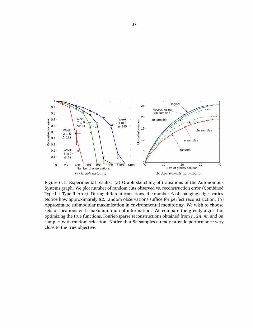
87
0 200 400 600 800 1000 1200 14000
0.1
0.2
0.3
0.4
0.5
0.6
0.7
0.8
0.9
1
Number of observations
Rec
onst
ruct
ion
erro
r
Week 7 to 9∆=161
Week1 to 3∆=245
Week5 to 7∆=62
Week3 to 5∆=122
(a) Graph sketching
0 10 20 30 400
5
10
15
20
25
Size of greedy solution
Mut
ual i
nfor
mat
ion
Original
random
n samples
2n samples
Approx. using8n samples
4n samples
(b) Approximate optimization
Figure 6.1: Experimental results. (a) Graph sketching of transitions of the AutonomousSystems graph. We plot number of random cuts observed vs. reconstruction error (CombinedType I + Type II error). During different transitions, the number ∆ of changing edges varies.Notice how approximately 8∆ random observations suffice for perfect reconstruction. (b)Approximate submodular maximization in environmental monitoring. We wish to choosesets of locations with maximum mutual information. We compare the greedy algorithmoptimizing the true functions, Fourier-sparse reconstructions obtained from n, 2n, 4n and 8nsamples with random selection. Notice that 8n samples already provide performance veryclose to the true objective.

88
As we have observed in Section 6.5, cut functions are contained in H2, and there is one
edge for each nonzero Fourier coefficient. We can thus use Corollary 6.1 to reconstruct the
graph by observing O (|k(t)| log4 n) values of random cuts, where k(t) is the number of edges
at time t. Note that while in practice, typically k = Ω(n), and for large graphs, we would
require a proportionally large number of observations. If, however, we are interested in
how a graph changes over time, and this change happens slowly, we use the fact that the
difference W(t) −W(t+1) is sparse.
In our experiments, we take a sequence of five snapshots of the Autonomous Systems
graph 1. Our experiments are performed on the subgraph induced by the 128 nodes with
largest degree. We first pick an increasing number of sets at random. We then sketch the
graphs at different time steps by computing the cut values associated with those sets. Since
the cut function is linear in the edge weights, the difference in cut values corresponds to
the cuts in the symmetric graph differences. We can therefore reconstruct the difference in
the edge sets by using the reconstruction algorithm described in Section 6.5. Note that the
number of changing edges varies from 62 to 245. Figure 6.1a presents the reconstruction
error (in terms of the fraction of edges correctly classified as changing or not changing). For
all transitions, exact recovery is possible, using a number of samples that is approximately a
factor of 8 larger than the number of changing edges. Also, we observe that, consistently,
with results in compressive sensing, a sharp phase transition occurs between a regime in
which the error is close to 100%, and the regime in which perfect reconstruction occurs.
6.6.2 Approximate submodular optimization
Suppose a submodular function to be optimized is extremely expensive to evaluate, but
can be approximated with our recontruction methods from random samples. Then one can
evaluate the function on random samples to construct an approximation, and optimize the
approximation. We test this approach on submodular function maximization in an environ-
mental monitoring application. We consider the problem of selecting a small number of most
informative observations for the purpose of spatial prediction. We take temperature data from
the NIMS sensor node [HAG+06] deployed at a lake near the University of California, Merced.
The environment is discretized in a set E of n = 86 locations. We train a nonstationary
Gaussian Process using data from a single scan of the lake by the NIMS sensor node, using a1downloaded from http://snap.stanford.edu

89
method described by [KSG08]. In order to quantify the informativeness of a set of locations
A∈ 2E , we use the mutual information
f (A) = I(XA; XE\A) = H(XE\A)−H(XE\A | XA)
that quantifies the reduction of uncertainty in the unobserved locations E \ A by taking
into account the observations XA at the selected observations. As shown by [KSG08], f is
submodular and approximately monotonic (for small sets A). Therefore, an efficient greedy
algorithm produces a set AG with near-maximal informativeness. The algorithm proceeds by
adding observations that maximally increase f (A) until k observations have been selected
[NWF78].
Unfortunately, computing mutual information f (A) for the case of Gaussian processes
requires solving a linear system of n variables, which is very expensive for large n. We
consider approximating f by a low-order function. We evaluate f on an increasing number
of sets, chosen uniformly at random, and then use the algorithm described in Section 6.5 to
approximate f ∈ H2. Notice that even though f not exactly sparse, it appears to be well-
approximated by a order 2 function: the best order 2 approximation explains approximately
86 % of its variance. In order to determine how well suited the approximate function is
for optimization, we run the greedy algorithm on the approximation, and compare the
resulting sets with the (provably near-optimal) solutions obtained by running the greedy
algorithm on the original (expensive to evaluate) function f . As baseline, we also compare
against the performance of sets chosen uniformly at random. Figure 6.1b presents the
results of the experiment, using approximations obtained from n, 2n, 4n and 8n random
function evaluations. Notice that n and 2n function evaluations, not surprisingly, lead to
poor performance. However, even 4n samples lead to strong performance, and 8n samples
leads to solutions almost as good as those obtained when working with the true objective.
These results indicate that the proposed approximations can perform very well even though
the assumption of exact sparsity in the Fourier domain is not met.
6.6.3 Synthetic Submodular Recovery
We claimed in Section 6.4 that if a function is known to be submodular, then incorporating
convex constraints implied by submodularity can improve the recovery of a function. We now
90
describe some experiments on synthetic functions that demonstrate this claim empirically.
We attempt the recovery a 3rd order submodular function by incorporating the constraints
from Equation 6.4.6 into a convex recovery algorithm.
We take n = 16 and restrict to H3, therefore p = 697. By Proposition 5, we can check
submodularity with 120 constraints. These numbers are small enough so that we can use a
standard interior point method solver to get accurate solutions. We construct f by taking a
function with i.i.d. Gaussian entries and then projecting it onto the cone H−2 ∩H3 to get a
target synthetic function. The resulting projection is not exactly sparse; on average it has
200± 10 (out of 697 possible) nonzero Fourier coefficients. However, it is compressible, and
so we can expect a small error even without recovering the support exactly. Then, given
random function samples, we reconstruct the target function by minimizing the Fourier `1
norm, but vary what sets of additional constraints we apply. First, we simply solve Equation
6.3.4 with no additional constraints. For our second way, we assume oracle access to the
signs of the Fourier coefficients and we enforce the known signs of the coefficients. Lastly,
we enforce the constraints of Equation 6.4.6. The results are plotted in Figure 2. Enforcing
submodularity significantly improves the recovery. It gives a relative error of less than 10−3
with only 300 measurements, and it recovers the support exactly with about 350. Using
the `1 norm alone requires about 450 measurements just to get a relative error or 10−3.
The method with oracle access to the signs of the coefficients has better performance than
standard `1, but is still not as good as the submodularity-enforcing method.
6.7 Related Work
Fourier analysis on the Boolean cube The problem of learning Boolean and pseudo-
boolean functions has a long history with many special cases that have been studied, and the
use of discrete Fourier analysis dates back to the work of [Man94] and [LMN93].
The specific problem of reconstructing graphs from few observations has received attention
due to important applications in bioinformatics. [AC04]. The literature distinguishes additive
queries (computing weight of all edges in a subgraph), and less powerful cross-additive queries
(computing the weight of edges between two sets of vertices). Cuts are a special case of
the latter. The literature also distinguishes adaptive queries (that can choose observations
based on past observations) and less powerful nonadaptive queries (that have to commit to all

91
50 100 150 200 250 300 350 400 450 5000
0.2
0.4
0.6
0.8
1Coefficient signs
known and enforced
3rd order submodularity known and enforced
Min l1 with no
additional constraint
Figure 6.2: Empirical study of submodular constraints. Synthetic functions on a base set of16 elements. Attempted recovery with differing types of constraints. The experiments wererepeated with different random synthetic functions and different random measurments, andthe mean relative error ‖ f − g‖2/‖ f ‖2 is plotted vs. number of random measurements.
observations in advance). In general, non-adaptive algorithms only requiring cross-additive
queries are preferred (as these make the fewest assumptions, can be parallelized, etc.). For
graphs with n nodes and k edges, an information theoretic lower bound of Ω k log(n2/k)
log k
additive (possibly adaptive) queries is known. [Maz10] provides an adaptive polynomial
time algorithm that attains this optimal complexity in log n nonadaptive rounds. To our
knowledge, the only existing non-adaptive algorithms with linear dependence on k are non-
constructive (i.e., not polynomial time) [BM10]. This approach also requires additive queries.
To our knowledge, ours is the first efficient nonadaptive approach (and furthermore only
requires cross-additive queries).
Learning of pseudo-boolean functions (and associated hypergraphs) has been considered
in [CJK11], which provides an almost tight adaptive algorithm for computing the Fourier
coefficients of k-bounded pseudoboolean functions. [BM10] provide a non-adaptive, but
also non-constructive approach, requiring additive queries.
Learning submodular functions Unfortunately, even without noise, there are strong lower
bounds, limiting our expectations on learning general submodular functions. Without access

92
to a data set of exponential size, it is not possible to approximate general submodular
functions to a factor better than Ω(p
n/ log n) [GHIM09]. On a more positive side, if the
function is Lipschitz, and sets are sampled uniformly at random, then for any ε > 0, a
O (log 1ε) approximation can be achieved on a fraction of at least 1− ε of all sets [BH11].
However, for optimization purposes, a guarantee that the approximation is of high quality
on only a subset (even a large subset) of sets is problematic, since typically nothing can be
inferred about the resulting minimizer. The problem of approximating a general submodular
function by a simpler one for the purpose of efficient minimization is studied in [JLB11],
who do not exploit the special structure of Fourier-sparse functions.
Compressive sensing There has been vast interest in sparse reconstruction and compressive
sensing [Don06, CW08]. But traditionally this has been motivated by sparsity of signals as a
trigonometric polynomial or in the wavelet domain. However, we are unaware of any work
directly applying these ideas to discrete cube. If work on sublinear Fourier transforms as of
[GGI+02] can be thought of as applying the ideas from learning sparse boolean functions
to sparse trigonmetric polynomials, then our work can be thought of as doing the reverse.
Opening up a toolbox of new methods for this domain is the main contribution of this chapter.
6.8 Conclusion
We have considered the problem of reconstructing set functions with decaying Fourier
(Hadamard-Walsh) spectrum, from a small number of possibly noisy observations. By lever-
aging recent results from random matrices and sparse reconstruction, we have shown that
standard algorithms can be used to obtain perfect reconstruction, with a number of samples
that scales linearly with the support size of the Fourier spectrum. This insight allows us to
open up a vast toolbox of modern optimization methods for learning set functions, which
previously has been mostly the domain of purely theoretical investigation. For example, our
results imply that standard `1 minimization can be used to reconstruct a sparse graph from
observing the values of a number of random cuts, which (up to logarithmic factors) matches
information-theoretic lower bounds in [Maz10]. Furthermore, we show that other properties,
such as submodularity and symmetry, imply structure among the Fourier coefficients that
can be exploited to reduce sample complexity, as well as speed up reconstruction algorithms.

93
We demonstrate the effectiveness of our approach on two applications, showing that we
can indeed sketch changes in real-world networks by measuring random cuts, and that we
can obtain useful approximations of expensive-to-compute set functions for the purpose of
optimization.
94
Chapter 7
Conclusion
One of our main objectives in this work has been to bridge the gap between the two extremes
of submodular functions: on one hand there are very basic or specialized functions that admit
simple and practical minimization algorithms, but are fairly limited in what they can describe,
and, on the other, there are the those for which no specialized minimization algorithms are
known. For the latter case, the only algorithms that have polynomial upper bounds on the
running time are impractical for all but very small problems, and the methods which seem
to work have no guarantees. Our intent has been to the extend the classes of submodular
functions for which there exist fairly efficient algorithms, and to that end in Chapter 4 and 5
we developed several novel techniques for submodular minimization using convex analysis.
The SLG algorithm of Chapter 4 gives a method for minimizing sums of functions of the
form φ(w(A)): these are compositions of nonnegative modular functions w with concave
functions φ. Admittedly, such functions are always representable as a minimum of a second
order submodular function, so in principle they can be solved via graph cut algorithms.
However, if the concave function φ is not piecewise linear, in order to represent the function
exactly, one needs to introduce a breakpoint (corresponding to an extra vertex in the graph)
for every possible value of w(A), which, in the worst case, is 2n. The main innovation of our
algorithm is that it remains efficient and independent of the number of breakpoints. We do
this by computing a gradient of a smoothed version of the Lovász extension and applying an
accelerated descent method.
In Chapter 5, our main result demonstrates that there is a great deal of flexibility in
choosing a barrier function to minimize a submodular function via convex programming. It
might be useful, in fact, to adapt the barrier function to the submodular function. In analogy
to matrix preconditioning: would this help address scaling issues, and how could we estimate

95
an appropriate choice for the barrier function?
The major question we attempted to address, and one which remains unresolved, is
how can we try to discover better representations of submodular functions? A common
theme of this thesis is the utility of having a simple description of the base polytope of a
submodular function. We expect such descriptions to be useful both for learning a submodular
function and projecting onto the base polytope (essentially the same problem as submodular
minimization).
Most of the functions in our experiments are variations of graph representable functions
such as in Equation 3.3.13. Our interest has not been in trying to extend graph cut algorithms
but to take advantage of the efficient base polytope representation of Equation 3.3.14. By
efficient, we mean refer to the fact that the number of variables and additional constraints
scales linearly with the number of nonzero coefficients in the specification. Can we find any
other classes of submodular functions that also have efficient lifted representations—possibly
in terms of the second order cone or the semidefinite cone? And if such classes exist, do
the any of results in Chapter 6 generalize to allow one to learn such a representation in a
reasonable time with a reasonable number of observations?
Lastly, we would like to pose one core question to that seems simple but remains open
to our knowledge—what is the smallest family of submodular functions such that every
submodular function is in their conic hull? Equivalently, what is the smallest number of
half-spaces that intersect to form the submodular polar cone
H−2
? We know this family
must exist, and it must be finite, albeit exponential in size.

96
Appendix A
Matroid Theory
Matroids are a class of set systems which are intimately connected to submodular set functions.
The name “matroid” stems from the fact that they can be treated as an abstract generalization
of matrices. However, there are several different equivalent definitions of matroids, some of
which are quite unexpected. For a gentle introduction to the subject, see [GM12]. Since our
focus is on submodularity, we give merely the original definition of matroid introduced by
Whitney [Whi35] (in terms of independent sets), as well as a formulation (in terms of the
existence of a rank function) which directly invokes submodularity.
A matroid M = (E,I) is defined by a ground set E together with a collection of subsets
I ⊆ 2E that satisfies the following properties:
Properties A.1. Matroid Independence Axioms
I-1. ; ∈ I
I-2. A⊂ B and B ∈ I ⇒ A∈ I
I-3. A, B ∈ I with |A|< |B| ⇒ ∃ b ∈ B \ A such that A+ b ∈ I
It is an exercise in elementary linear algebra to show that if E is a set of vectors from
a common vector space, then the collection of independent subsets of vectors satisfies the
Properties A.1. For general matroids, the sets in the collection I are called the independent
sets of a matroid. If a set of vectors are expressed in the form of a matrix, and the independent
sets of those vectors are in one-to-one correspondence with the independent sets of a matroid,
then that matrix is said to represent the matroid. Matroids are strictly more general than
matrices in that not every matroid can be represented as a matrix, though the simplest
example requires |E| ≥ 8.

97
An alternative characterization of a matroid is through the properties of an associated set
function. One can show that a set E is the ground set for a matroid if and only if it admits a
set function r ∈H with the following properties:
Properties A.2. Matroid Rank Axioms
R-1. r(;) = 0.
R-2. r(A+ b)− r(A) ∈ 0, 1 for all A∈ 2E , b ∈ E \ A.
R-3. r(A+ b+ c)− r(A+ b)− r(A+ c) + r(A)≤ 0 for all A∈ 2E , b, c ∈ E \ A.
Of particular note is the third property: submodularity.
As an example, if E is a set of vectors, then the Properties A.2 are satisfied by the set
function equal to the dimension of the subspace spanned by vectors in a set (a.k.a. the rank).
For general matroids, the rank of a set is defined as the size of the largest independent subset:
r(A) =maxB∈IB⊆A
|B| (A.0.1)
One can check that for any matroid, the rank function defined this way gives rise to a set
function satisfying Properties A.2.
Conversely, given a rank function satisfying Properties A.2, one can define independent
sets as those whose size equals their rank:
I= A∈ 2E | r(A) = |A| (A.0.2)
Then one can check that this collection forms the independence system of a matroid; that is,
Properties A.1 are satisfied.
Other defining features of matroids are their circuits (minimal dependent sets) and their
bases (maximal independent sets). The latter is significant for the theory of submodular
functions, since the set of bases of a matroid forms corresponds to the vertices of the base
polytope (as defined in Equation 3.3.2) of the rank function.
One extremely important generalization of matroids are polymatroids, as introduced by
Edmonds [Edm70]. If the independence system of a matroid is considered to be a subset
of the Boolean cube 0, 1n, then a polymatroid is an analogous subset of Zn+ or Rn
+. In the

98
case of real vectors, it is equivalent to the base polytope of a nonnegative nondecreasing
submodular function.
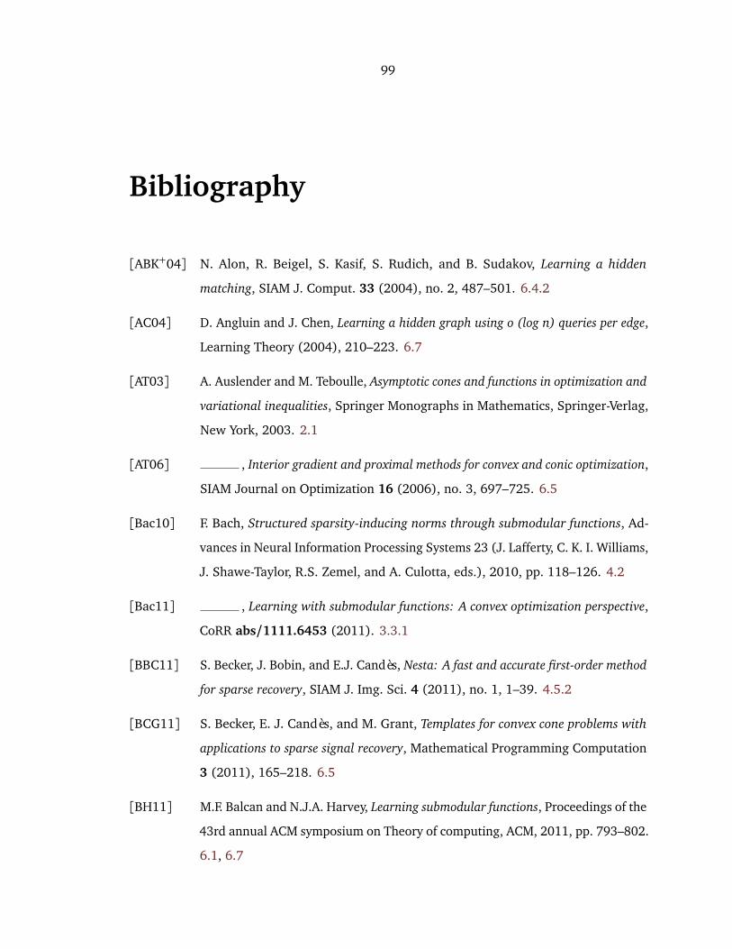
99
Bibliography
[ABK+04] N. Alon, R. Beigel, S. Kasif, S. Rudich, and B. Sudakov, Learning a hidden
matching, SIAM J. Comput. 33 (2004), no. 2, 487–501. 6.4.2
[AC04] D. Angluin and J. Chen, Learning a hidden graph using o (log n) queries per edge,
Learning Theory (2004), 210–223. 6.7
[AT03] A. Auslender and M. Teboulle, Asymptotic cones and functions in optimization and
variational inequalities, Springer Monographs in Mathematics, Springer-Verlag,
New York, 2003. 2.1
[AT06] , Interior gradient and proximal methods for convex and conic optimization,
SIAM Journal on Optimization 16 (2006), no. 3, 697–725. 6.5
[Bac10] F. Bach, Structured sparsity-inducing norms through submodular functions, Ad-
vances in Neural Information Processing Systems 23 (J. Lafferty, C. K. I. Williams,
J. Shawe-Taylor, R.S. Zemel, and A. Culotta, eds.), 2010, pp. 118–126. 4.2
[Bac11] , Learning with submodular functions: A convex optimization perspective,
CoRR abs/1111.6453 (2011). 3.3.1
[BBC11] S. Becker, J. Bobin, and E.J. Candès, Nesta: A fast and accurate first-order method
for sparse recovery, SIAM J. Img. Sci. 4 (2011), no. 1, 1–39. 4.5.2
[BCG11] S. Becker, E. J. Candès, and M. Grant, Templates for convex cone problems with
applications to sparse signal recovery, Mathematical Programming Computation
3 (2011), 165–218. 6.5
[BH11] M.F. Balcan and N.J.A. Harvey, Learning submodular functions, Proceedings of the
43rd annual ACM symposium on Theory of computing, ACM, 2011, pp. 793–802.
6.1, 6.7
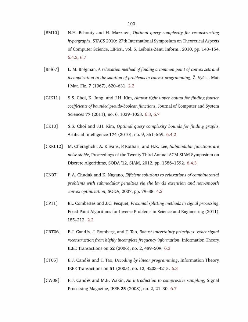
100
[BM10] N.H. Bshouty and H. Mazzawi, Optimal query complexity for reconstructing
hypergraphs, STACS 2010: 27th International Symposium on Theoretical Aspects
of Computer Science, LIPIcs., vol. 5, Leibniz-Zent. Inform., 2010, pp. 143–154.
6.4.2, 6.7
[Brè67] L. M. Brègman, A relaxation method of finding a common point of convex sets and
its application to the solution of problems in convex programming, Z. Vycisl. Mat.
i Mat. Fiz. 7 (1967), 620–631. 2.2
[CJK11] S.S. Choi, K. Jung, and J.H. Kim, Almost tight upper bound for finding fourier
coefficients of bounded pseudo-boolean functions, Journal of Computer and System
Sciences 77 (2011), no. 6, 1039–1053. 6.3, 6.7
[CK10] S.S. Choi and J.H. Kim, Optimal query complexity bounds for finding graphs,
Artificial Intelligence 174 (2010), no. 9, 551–569. 6.4.2
[CKKL12] M. Cheraghchi, A. Klivans, P. Kothari, and H.K. Lee, Submodular functions are
noise stable, Proceedings of the Twenty-Third Annual ACM-SIAM Symposium on
Discrete Algorithms, SODA ’12, SIAM, 2012, pp. 1586–1592. 6.4.3
[CN07] F. A. Chudak and K. Nagano, Efficient solutions to relaxations of combinatorial
problems with submodular penalties via the lovász extension and non-smooth
convex optimization, SODA, 2007, pp. 79–88. 4.2
[CP11] P.L. Combettes and J.C. Pesquet, Proximal splitting methods in signal processing,
Fixed-Point Algorithms for Inverse Problems in Science and Engineering (2011),
185–212. 2.2
[CRT06] E.J. Candès, J. Romberg, and T. Tao, Robust uncertainty principles: exact signal
reconstruction from highly incomplete frequency information, Information Theory,
IEEE Transactions on 52 (2006), no. 2, 489–509. 6.3
[CT05] E.J. Candès and T. Tao, Decoding by linear programming, Information Theory,
IEEE Transactions on 51 (2005), no. 12, 4203–4215. 6.3
[CW08] E.J. Candès and M.B. Wakin, An introduction to compressive sampling, Signal
Processing Magazine, IEEE 25 (2008), no. 2, 21–30. 6.7

101
[Don06] D.L. Donoho, Compressed sensing, Information Theory, IEEE Transactions on 52
(2006), no. 4, 1289–1306. 6.3, 6.7
[DSSSC08] J. Duchi, S. Shalev-Shwartz, Y. Singer, and T. Chandra, Efficient projections onto
the l1-ball for learning in high dimensions, Proceedings of the 25th international
conference on Machine learning, ICML ’08, 2008, pp. 272–279. 5.4.2
[Edm70] J. Edmonds, Submodular functions, matroids, and certain polyhedra, Combina-
torial Structures and their Applications (Proc. Calgary Internat. Conf., Calgary,
Alta., 1969), Gordon and Breach, New York, 1970, pp. 69–87. 1, 3.3.1, 3.3.2, A
[EVGW+] M. Everingham, L. Van Gool, C.K.I. Williams, J. Winn, and A. Zisserman, The PAS-
CAL Visual Object Classes Challenge 2009 (VOC2009) Results, http://www.pascal-
network.org/challenges/VOC/voc2009/workshop/index.html. 4.7
[FD05] D. Freedman and P. Drineas, Energy minimization via graph cuts: settling what
is possible, Computer Vision and Pattern Recognition, 2005. CVPR 2005. IEEE
Computer Society Conference on, vol. 2, june 2005, pp. 939 – 946 vol. 2. 4.1
[FH05] S. Foldes and P.L. Hammer, Submodularity, Supermodularity, and Higher-Order
Monotonicities of Pseudo-Boolean Functions, Mathematics of Operations Research
30 (2005), no. 2, 453. 3.2.2
[FI03] L. Fleischer and S. Iwata, A push-relabel framework for submodular function
minimization and applications to parametric optimization, Discrete Appl. Math.
131 (2003), no. 2, 311–322, Submodularity. 4.7
[FI11] S. Fujishige and S. Isotani, A submodular function minimization algorithm based
on the minimum-norm base, Pac. J. Optim. 7 (2011), no. 1, 3–17. 3.4.2, 4.7
[Fis67] P.C. Fishburn, Interdependence and additivity in multivariate, unidimensional
expected utility theory, International Economic Review 8 (1967), no. 3, 335–342.
6.1
[Fou10] S. Foucart, A note on guaranteed sparse recovery via âDS1-minimization, Applied
and Computational Harmonic Analysis 29 (2010), no. 1, 97–103. 6.3

102
[Fuj05] S. Fujishige, Submodular functions and optimization, second ed., Annals of
Discrete Mathematics, vol. 58, Elsevier B. V., Amsterdam, 2005. MR 2171629
(2006d:90098) 3.3, 3.3.1
[GGI+02] A.C. Gilbert, S. Guha, P. Indyk, S. Muthukrishnan, and M. Strauss, Near-optimal
sparse fourier representations via sampling, Proc. STOC, 2002. 6.7
[GHIM09] M.X. Goemans, N.J.A. Harvey, S. Iwata, and V. Mirrokni, Approximating sub-
modular functions everywhere, Proceedings of the twentieth Annual ACM-SIAM
Symposium on Discrete Algorithms, Society for Industrial and Applied Mathe-
matics, 2009, pp. 535–544. 6.1, 6.7
[GK00] V. Grebinski and G. Kucherov, Optimal Reconstruction of Graphs under the Additive
Model., Algorithmica 28 (2000), no. 1, 104–124. 6.4.2
[GLS81] M. Grötschel, L. Lovász, and A. Schrijver, The ellipsoid method and its consequences
in combinatorial optimization, Combinatorica 1 (1981), no. 2, 169–197. 1, 3.3.2,
3.4.1
[GM12] G. Gordon and J. McNulty, Matroids: a geometric introduction, Cambridge Uni-
versity Press, Cambridge, 2012. A
[GMR00] M. Grabisch, J.L. Marichal, and M. Roubens, Equivalent representations of set
functions, Mathematics of Operations Research 25 (2000), no. 2, 157–178. 3.2.3,
3.2.4
[Hac79] L.G. Hacijan, A polynomial algorithm in linear programming, Dokl. Akad. Nauk
SSSR 244 (1979), no. 5, 1093–1096. 3.4.1
[HAG+06] T.C. Harmon, R.F. Ambrose, R.M. Gilbert, J.C. Fisher, M. Stealey, and W.J. Kaiser,
High Resolution River Hydraulic and Water Quality Characterization using Rapidly
Deployable Networked Infomechanical Systems (NIMS RD), Tech. Report 60, CENS,
2006. 6.6.2
[HH92] P.L. Hammer and R. Holzman, Approximations of pseudo-Boolean functions; ap-
plications to game theory, ZOR Zeitschrift für Operations Research Methods and
Models of Operations Research 36 (1992), no. 1, 3–21. 3.2.3

103
[HUL93] Jean-Baptiste Hiriart-Urruty and Claude Lemaréchal, Convex analysis and mini-
mization algorithms. II, Grundlehren der Mathematischen Wissenschaften [Fun-
damental Principles of Mathematical Sciences], vol. 306, Springer-Verlag, Berlin,
1993, Advanced theory and bundle methods. 2.1
[IFF01] S. Iwata, L. Fleischer, and S. Fujishige, A combinatorial strongly polynomial
algorithm for minimizing submodular functions, J. ACM 48 (2001), no. 4, 761–
777. 1, 3.4.1
[II07] T. Itoko and S. Iwata, Computational geometric approach to submodular func-
tion minimization for multiclass queueing systems, Integer Programming and
Combinatorial Optimization (Matteo Fischetti and DavidP. Williamson, eds.),
Lecture Notes in Computer Science, vol. 4513, Springer Berlin Heidelberg, 2007,
pp. 267–279. 4.3, 4.4.3
[IO09] S. Iwata and J. B. Orlin, A simple combinatorial algorithm for submodular function
minimization, Proceedings of the twentieth Annual ACM-SIAM Symposium on
Discrete Algorithms (Philadelphia, PA, USA), SODA ’09, Society for Industrial
and Applied Mathematics, 2009, pp. 1230–1237. 1, 3.4.1
[JLB11] Stefanie Jegelka, Hui Lin, and Jeff A. Bilmes, On fast approximate submodular
minimization, Advances in Neural Information Processing Systems 24 (J. Shawe-
Taylor, R.S. Zemel, P. Bartlett, F.C.N. Pereira, and K.Q. Weinberger, eds.), 2011,
pp. 460–468. 3.4.3, 6.7
[JM93] D.S. Johnson and C.C. McGeoch (eds.), Network flows and matching: First dimacs
implementation challenge, American Mathematical Society, Boston, MA, USA,
1993. 4.1, 4.7
[KK80] A.K. Kelmans and B.N. Kimelfeld, Multiplicative submodularity of a matrix’s prin-
cipal minor as a function of the set of its rows and some combinatorial applications,
Discrete Mathematics 44 (1980), no. 1, 113–116. 6.1
[KKT07] P. Kohli, M.P. Kumar, and P.H.S. Torr, P3 beyond: Solving energies with higher
order cliques, Computer Vision and Pattern Recognition, 2007. CVPR ’07. IEEE
Conference on, june 2007, pp. 1 –8. 4.3

104
[KLT09] P. Kohli, L. Ladický, and P.H. Torr, Robust higher order potentials for enforcing label
consistency, Int. J. Comput. Vision 82 (2009), no. 3, 302–324. 4.3
[Kra10] A. Krause, Sfo: A toolbox for submodular function optimization, J. Mach. Learn.
Res. 11 (2010), 1141–1144. 4.7
[KSG08] A. Krause, A. Singh, and C. Guestrin, Near-Optimal Sensor Placements in Gaussian
Processes: Theory, Efficient Algorithms and Empirical Studies, Journal of Machine
Learning Research 9 (2008), 235–284. 6.1, 6.6.2
[KZ04] V. Kolmogorov and R. Zabin, What energy functions can be minimized via graph
cuts?, Pattern Analysis and Machine Intelligence, IEEE Transactions on 26 (2004),
no. 2, 147–159. 3.4.3
[LMN93] N. Linial, Y. Mansour, and N. Nisan, Constant depth circuits, Fourier transform,
and learnability, Journal of the ACM (JACM) 40 (1993), no. 3, 607–620. 6.7
[Lov83] L. Lovász, Submodular functions and convexity, Mathematical programming: the
state of the art, Springer, Berlin, 1983, pp. 235–257. 1, 3.3.2, 4.2, 4.2, 4.2, 6.1,
6.4.3
[Man94] Y. Mansour, Learning boolean functions via the fourier transform, Theoretical
advances in neural computation and learning (1994), 391–424. 6.7
[Maz10] H. Mazzawi, Optimally reconstructing weighted graphs using queries, Proc. SODA,
2010. 6.7, 6.8
[Mur03] K. Murota, Discrete convex analysis, SIAM Monographs on Discrete Mathemat-
ics and Applications, Society for Industrial and Applied Mathematics (SIAM),
Philadelphia, PA, 2003. 1
[Nes05] Y. Nesterov, Smooth minimization of non-smooth functions, Mathematical Pro-
gramming 103 (2005), 127–152. 4.1, 4.2, 4.5.2, 4.5.2
[NWF78] G.L. Nemhauser, L.A. Wolsey, and M.L. Fisher, An analysis of approximations for
maximizing submodular set functions - I, Mathematical Programming 14 (1978),
no. 1, 265–294. 3.3, 6.6.2

105
[PK90] P.M. Pardalos and N. Kovoor, An algorithm for a singly constrained class of
quadratic programs subject to upper and lower bounds, Mathematical Program-
ming 46 (1990), 321–328. 5.4.2
[Que98] M. Queyranne, Minimizing symmetric submodular functions, Mathematical Pro-
gramming 82 (1998), 3–12. 3.4.3, 4.1
[Rau10] H. Rauhut, Compressive sensing and structured random matrices, Theoretical
foundations and numerical methods for sparse recovery, Radon Ser. Comput.
Appl. Math., vol. 9, Walter de Gruyter, Berlin, 2010, pp. 1–92. 6.3
[Roc70] R.T. Rockafellar, Convex analysis, Princeton Mathematical Series, No. 28, Prince-
ton University Press, Princeton, N.J., 1970. 2.1
[RV08] M. Rudelson and R. Vershynin, On sparse reconstruction from Fourier and Gaussian
measurements, Communications on Pure and Applied Mathematics 61 (2008),
no. 8, 1025–1045. 6.3
[Sch03] A. Schrijver, Combinatorial optimization. Polyhedra and efficiency. Vol. B, Algo-
rithms and Combinatorics, vol. 24, Springer-Verlag, Berlin, 2003, Matroids, trees,
stable sets, Chapters 39–69. 3.3.1, 6.1
[SK10] P. Stobbe and A. Krause, Efficient minimization of decomposable submodular
functions, NIPS, 2010, pp. 2208–2216. 1.1, 1.2
[SK12] , Learning fourier sparse set functions, Journal of Machine Learning Re-
search - Proceedings Track 22 (2012), 1125–1133. 1.2
[SWRC09] J. Shotton, J. Winn, C. Rother, and A. Criminisi, Textonboost for image under-
standing: Multi-class object recognition and segmentation by jointly modeling
texture, layout, and context, International Journal of Computer Vision 81 (2009),
2–23. 4.3, 4.7
[Tro04] J.A. Tropp, Greed is good: algorithmic results for sparse approximation., IEEE
Transactions on Information Theory 50 (2004), no. 10, 2231–2242. 6.5
[TW10] J.A. Tropp and S.J. Wright, Computational Methods for Sparse Solution of Linear
Inverse Problems, Proceedings of the IEEE 98 (2010), no. 6, 948–958. 6.5

106
[Ver12] R. Vershynin, Introduction to the non-asymptotic analysis of random matrices,
Compressed sensing, Cambridge Univ. Press, Cambridge, 2012, pp. 210–268.
6.1, 6.3
[Whi35] H. Whitney, On the Abstract Properties of Linear Dependence, Amer. J. Math. 57
(1935), no. 3, 509–533. A