Converting Unstructured into Semi-StructuredProcess Models

Rik Eshuisa, Akhil Kumarb

aEindhoven University of Technology, School of Industrial EngineeringP.O. Box 513, 5600 MB Eindhoven, The Netherlands

bDepartment of Supply Chain and Information Systems, Smeal College of Business, PennState University, University Park, PA 16802, USA

Abstract

Business process models capture process requirements that are typically ex-pressed in unstructured, directed graphs that specify parallelism. However,modeling guidelines or requirements from execution engines may require thatprocesses models are structured in blocks. The goal of this paper is to define anautomated method to convert an unstructured process model containing paral-lelism into an equivalent semi-structured process model, which contains blocksand synchronization links between parallel branches. We define the method bymeans of an algorithm that is based on dominators, a well-known techniquefrom compiler theory for structuring sequential flow graphs. The method runsin polynomial time. We implemented and evaluated the algorithm extensively.In addition we compared the method in detail with the BPStruct method fromliterature. The comparison shows that our method can handle cases that BP-Struct is not able to and that the method coincides with BPStruct for the casesthat BPStruct is able to handle.

Keywords: Business process management, process models, semi-structuredprocesses, model transformation.

1. Introduction

Business processes management (BPM) [1, 2] focuses on the automation ofbusiness processes using middleware information technology. Business processmodels play a key role in BPM. They can be conceptual-level designs of businessprocesses, but they can also specify the coordination logic for execution enginesthat support the operational management of business processes. Communi-cation of business process models between different stakeholders, end users orsystem engineers is of utmost importance to realize a successful implementation.

An important subclass of process models are structured process models,which consist of nested blocks and each block has a single entry point and

Email addresses: h.eshuis@tue.nl (Rik Eshuis), akhilkumar@psu.edu (Akhil Kumar)

Preprint submitted to Elsevier November 3, 2015

2

a single exit point. Examples of structured languages are the Business Pro-cess Execution Language (BPEL) [3] and OWL-S [4], a language for describingsemantic web services using the Web Ontology Language (OWL). Structuredprocess models are also required by advanced BPM techniques such as processviews in inter-organizational collaborations [5, 6], rule-driven implementationsof process models [7], and dynamic changes of running processes [8].

A structured process model is similar to a (parallel) program without gotostatements. While every unstructured program has a structured equivalent [9],this is not true for unstructured process models, since synchronization linksbetween parallel blocks cannot be expressed in a structured process model [10,11]. Therefore, established BPM languages like BPEL [3] and Adept [8] allowsemi-structured process models, which are structured into blocks with additionalsynchronization links between parallel blocks.

Structured process models are easier to read and understand than unstruc-tured models [12] and contain fewer errors [13]. Structuredness has been pro-posed as modeling guideline [14]. But business processes are typically modeledin graph-based notations such as BPMN [15] or UML activity diagrams [16] thatdo not syntactically enforce structuredness. A graphical representation enableseasy communication with end-users in the organization in which the process isused. Nodes are either activities (tasks) or routing constructs like a choice splitor a parallel join while edges represent ordering constraints.

In a structured process graph, each split has a matching join, and the splitand join demarcate a subprocess that corresponds to a single-entry, single-exitblock. Since a split does not need to have a matching join, process graphs areusually not structured into blocks. Therefore translations have been proposedto structure graph-based process models [11, 17, 18]. But these approaches dono construct semi-structured process models.

We aim to define an automated method for converting an unstructuredprocess model into an equivalent semi-structured process model The method isdescribed as a formal algorithm, using well-known concepts from the field ofcompiler design [19] for structuring control flow graphs. However, a control flowgraph only specifies sequential behavior while a process model also specifies par-allel behavior, which complicates the structuring procedure. Another differenceis that the approach allows the identification of semi-structured process modelsin which parallel branches use cross-synchronization.

For every input process model, the method delivers output, but the resultis only meaningful (i.e., the output process is equivalent to the input process)if the input process model is correct, i.e., it is free of deadlocks and there is nolack of synchronization (see Section 3). Moreover, the approach only outputs asemi-structured process model if no equivalent structured process model exists.

Compared to existing approaches for structuring unstructured process mod-els [11, 17, 18], our method is more powerful, since it can generate both struc-tured and semi-structured processes, while existing approach can only generatestructured processes and fail for correct process models that have no equivalentstructured process. The overall time complexity of the method is polynomial,which ensures that the method scales well to large process models. Other ap-

3

proaches are either as efficient but less powerful [11, 17] or have a much highertime complexity [18]. An extensive discussion of related work can be found inSection 7.

To simplify the presentation, we restrict ourselves in the main text to acyclicprocess models. In the Appendix, we extend the algorithms of the main textto deal with cyclic process models in which each loop has a single entry and asingle exit point. Other papers [20, 21, 22] already discuss techniques to turna process model with unstructured loops into an equivalent process model inwhich each loop has a single entry and a single exit point. These techniques arecomplementary to our method and can be easily integrated.

The rest of this paper is organized as follows. Section 2 presents a motivatingexample. Section 3 defines process flow graphs, which formalize business processmodels, and a functional notation for representing semi-structured processes.To simplify the definition of the structuring algorithm, we apply in Section 4preprocessing steps to the input process flow graphs. Section 5 defines thestructuring algorithm that transforms a process flow graph into an equivalentsemi-structured process. The correctness of the algorithm is also analyzed inSection 5. To simplify the exposition, we consider acyclic process flow graphs inSection 4 and 5. Appendix A explains how the algorithm extends to process flowgraphs with loops. Section 6 discusses evaluation of the method. To evaluatefeasibility, we have implemented a prototype implementation of the method. Toevaluate the utility, we have applied the method to several benchmark examplestaken from the literature. Section 7 discusses related work. Finally, Section 8concludes this paper and gives directions for further work.

2. Motivating example

We motivate the approach with an example process model shown in Figure 1.The notation is explained in the next section. The process is about handlinginsurance claims for damaged vehicles. Each received claim is assessed. Forsmall amounts, the claim is accepted without further ado. For large paymentamounts, the vehicle is inspected and the payment is determined and approvedby a manager. In both cases, the claim is paid and in parallel a decision letter issent, where the decision is subject to the manager approval for large amounts.In parallel, each assessed claim is monitored and a report is created. Finally,the claim is archived if all previous tasks have completed.

The resulting process flow graph in Figure 1 cannot be converted into astructured process since there is a cross-synchronization between two parallelbranches (arrow from AND split A3 to AND join A4). Therefore, all existingapproaches for structuring process flow graphs [11, 17, 18] fail for this example.

The approach defined in this paper converts the process flow graph intothe semi-structured process shown in Figure 2. The synchronization constraintbetween A3 and A4 in Figure 1 is translated into condition done(A3) for taskFile report in Figure 2, where A3 is a dummy task whose sole purpose is to ensurethat File report starts at the proper moment. In the remainder of this paper, werevisit this example to explain and highlight key elements of the approach.

4

A1

X1

A2 A3X2

A5 X3

A6

A4

Figure 1: Process flow graph

[done(A3)]

Figure 2: Semi-structured process for Figure 1

3. Preliminaries

We define semi-structured process flow graphs. We also introduce definitionsbased on dominators from compiler theory [19] to identify structure in processflow graphs. These definitions are used in the structuring algorithm presentedin the next section.

3.1. Process flow graphs

We define a process flow graph as a generalization of a program flow graph [19].The main difference is that process flow graphs allow parallelism, while programflow graphs are strictly sequential.

A process flow graph P is a tuple (N,T,A,X, start, end,E, synch) where

– N is a set of nodes, partitioned in sets T , A, X, and {start, end}.

– T is a set of tasks,

– A is a set of AND connector nodes,

– X is a set of XOR connector nodes,

5

– start is the unique start node,

– end is the unique end node,

– E ⊆ N ×N is the control flow (transition) relation,

– synch ∶ N → BExp is a partial function that maps nodes to synchroniza-tion conditions, which are boolean expressions of set BExp. In the figures,each synchronization condition is demarcated with square brackets. Syn-chronization conditions only exist for semi-structured processes, definedbelow, not for unstructured processes.

For process flow graphs we use some standard definitions from graph the-ory [23]. If (n1, n2) ∈ E, then n1 is predecessor of n2 and n2 is successor of n1.A directed path is a sequence of nodes n1n2..nl such that for every i, 0 ≤ i < l,(ni, ni+1) ∈ E.

We use the following syntactic constraints on process flow graphs. As usualfor program flow graphs, we require that node start has no incoming edges,node end no outgoing edges, and each node in N lies on a directed path fromstart to end. Moreover, each task node should have exactly one incoming andone outgoing edge; start has one outgoing edge but no incoming edge; and endhas one incoming edge but no outgoing edge.

Next, we identify several other kinds of nodes in process flow graphs. Anode with more than one outgoing edge is called a split node. A node withmore than one incoming edge is called a join node. Since we require that thestart, end and task nodes have at most one incoming and one outgoing edge,each split and each join node is always an AND or a XOR connector node. Tosimplify the presentation, we require that a split node is not also a join node.For technical reasons, we do allow that an AND or XOR node is neither a splitnor a join, in which case it has one incoming and one outgoing edge.

Semi-structured process flow graphs

Structured process graphs are graphs with the property that the (AND andXOR) control nodes occur in (split, join) pairs, and these pairs are properlynested inside each other [11]. Each pair demarcates a block with a single entryand a single exit point. For such graphs we can represent blocks in a simplefunctional notation using A and X as pairs of AND and XOR splits respectively,and ‘;’ as the sequence operator. Semi-structured process graphs are structuredprocess graphs that use synchronization conditions on tasks, specified with func-tion synch. The synchronization condition of a task restricts when the task isallowed to start. Synchronization conditions are expressed in square brackets.Thus, the semi-structured process of Figure 2 is expressed in our notation as:

Start; Assess claim; P(Monitor claim; File report [done(A3)], X(Inspectvehicle; A3; P(Send decision, Approve payment; Pay), Accept claim;A3; P(Send decision, Pay))); Activate; End

6

Notice how the synchronization condition done(A3) appears next to File re-port task indicating that it is a precondition for this task. This notation isconvenient for textual representation. Given a process flow graph in this nota-tion it is straightforward to convert it to its visual representation.

Visualization

We visualize process flow graphs using the Business Process Modeling Nota-tion (BPMN)[15]. Rectangles represent tasks, a circle represents start, a circlewith a bold border represents end, AND nodes are represented by diamondswith a ‘+’ , and XOR nodes by diamonds with an ‘X’.

Correctness

A process flow graph can be incorrect in the sense that during execution itmay get stuck. Sadiq and Orlowska [24] have identified two correctness proper-ties for process models that apply directly to process flow graphs as well. Theyuse the auxiliary notation of an instance subgraph, which is a maximal sub-graph such that for each XOR node in the subgraph, one predecessor and onesuccessor is also in the subgraph, and for each AND node all predecessors andsuccessors are in the subgraph. An instance subgraph contains a deadlock ifit contains some predecessor nodes of an AND node but not all. An instancesubgraph has lack of synchronization if it contains more than one predecessornode of a XOR join.

A process flow graph is correct if each instance subgraph derived from it hasno deadlock and no lack of synchronization. More elabore and precise definitionscan be found elsewhere [24, 25]. These citations also contain efficient approachesfor verifying correctness. Structured process models are by construction correct.For the remainder of this paper, we only consider correct process flow graphs.

3.2. Identifying structure in process flow graphs

We introduce mathematical notions on process flow graphs that help todefine the structuring algorithm in Section 5. The notions build on the well-known concept of a dominator [19].

For a process flow graph (N,T,A,X, start, end,E, grd), node p dominatesanother node q ≠ p if every path from start to q passes through p. Node p isthe immediate dominator of node q, if p ≠ q and every dominator of q otherthan p also dominates p. Let IDOM(q) denote the immediate dominator of q.Symmetrically, node p post-dominates a node q ≠ p, if every path from q to endpasses through p. Let IPDOM(q) denote the unique immediate post-dominatorof q, so every post-dominator of q other than p also post-dominates IPDOM(q).The immediate dominator and immediate post-dominator are unique [19].

Example 1. Figure 3 shows the dominators for Figure 1 in a dominator tree [19].In the tree, each parent of a child is the immediate dominator of that child. Ina similar way, post-dominators can be represented in a tree. For instance, theimmediate post-dominator of A1 is A3. ◻

7

X1

Assess claim

File report Accept claim

A5

Inspect vehicle

A4

start

X3X2

Send decision

Pay

A6

Archive

end

A1

Monitor claim

A2 A3

Approve payment

Figure 3: Dominator tree for Figure 1

Table 1: FOLLOW sets for nodes in Figure 1

Node n FOLLOW (n) Node n FOLLOW (n)

start {Assess claim } A3 ∅

Assess claim {A1} Send decision ∅

A1 {A6} Approve payment ∅

Monitor claim ∅ Accept claim {A5}A4 {File report} A5 ∅

File report ∅ X3 {Pay}X1 ∅ Pay ∅

Inspect vehicle {A2} A6 {Archive}A2 ∅ Archive endX2 {A3} end ∅

We use IDOM and IPDOM to identify for each node n a set FOLLOW (n)containing its successor nodes at the same level of nesting in the structuredprocess model. For each node n1, n2 ∈ N , let

FOLLOW (n1) = { n2 ∣ n1 = IDOM(n2) ∧ n2 = IPDOM(n1) }.

If n1 is a split node and n1 = IDOM(n2), node n2 must have two or moreincoming edges, hence it is a join. The split and join can have different types.

If FOLLOW (n1) = {n2} for n1, n2 ∈ N , then the pair n1, n2 demarcates asingle entry single exit (SESE) region, where n1 is the entry node and n2 theexit node. However, set FOLLOW (n1) can be empty, as the following exampleillustrates.

Example 2. Consider the process flow graph in Figure 1. Table 1 shows theFOLLOW sets for the nodes in the process flow graph.

8

Table 2: Properties satisfied by acyclic process flow graphs

Property Definition How satisfied?

P1 For each pair of distinct nodes n1, n2,FOLLOW (n1) ∩ FOLLOW (n2) = ∅

By default

P2 For each node n, ∣FOLLOW (n)∣ ≤ 1 By defaultP3 For each split s, there is no join j such that

(s, j) is an edge in ERefactoring transi-tive edges

P4 For each AND join j, there is a split s such thatj ∈ FOLLOW (s)

Removing cross-synchronization

1: procedure Preprocess(P)2: P ∶= RemoveTransitiveEdges(P)3: P ∶= InsertSplits(P)4: P ∶= RemoveCrossSynchronization(P)5: P ∶= InsertSplits(P)6: end procedure

Figure 4: Preprocessing algorithm

Note that FOLLOW sets were introduced by Baker [26] for program flowgraphs. We adapted the definition slightly: the original definition does notrequire that for a split node n, each node in FOLLOW (n) post-dominates n.Consequently, the original definition allows that a split node has more thanone node in set FOLLOW . The definition allows the structuring algorithmdescribed in Section 5 to duplicate nodes, which is not catered for by the originalstructuring algorithm of Baker.

Table 2 lists properties of FOLLOW that are important for the algorithmdescribed in Section 5. Properties P3 and P4 only hold after applying prepro-cessing steps defined in Section 4. In Appendix B we prove that the propertieshold.

4. Preprocessing

We outline three preprocessing steps that have to be applied to an unstruc-tured process model before invoking the structuring algorithm described in thenext section (see Figure 4).

4.1. Refactoring transitive edges

Consider a split s and join j. If there is an edge (s, j) in E, and a path pfrom s to j that does not include (s, j), then edge (s, j) represents a transitiverelation, and we therefore call (s, j) transitive. To simplify the definition of thealgorithm in the next section, we refactor all transitive edges (Figure 5).

If s is an AND split, then transitive edge (s, j) is redundant and is thereforeremoved. If s is an XOR split, then (s, j) specifies a bypass edge: by taking(s, j) join j can be reached directly and the other nodes on path p are passed by.

9

1: procedure RefactorTransitiveEdges(P)2: for each transitive edge (s, n) ∈ E do3: remove (s, n) from E4: if s is a XOR split then5: d ∶= a dummy task such that d ∉ T6: T ∶= T ∪ {d}7: E ∶= E ∪ {s, d), (d,n)}8: end if9: end for

10: return P11: end procedure

Figure 5: Algorithm for removing transitive edges

A bypass edge is similar to an empty else-clause inside an if-then-else statement.For each bypass edge (s, j), we insert a dummy task d between s and j, andreplace edge (s, j) with edges (s, d) and (d, j).

After this preprocessing step, the process flow graph satisfies P3 (cf. Table 2).

4.2. Inserting splits

If a join j does not occur in the FOLLOW set of any (split) node, sometimesa split s can be inserted such that j ∈ FOLLOW (s). Each join has, by definition,an immediate dominator s, so s = IDOM(j), that is a split. An extra split s′

can be inserted immediately after s such that FOLLOW (s′) = {j}. Splits s′

gets the same connector type as s, so either s, s′ ∈ A or s, s′ ∈X.

Example 3. In Figure 6(a), AND join A2 is not in the FOLLOW set of ANDsplit A1, but A1 is the immediate dominator of A2. AND split A4 can be insertedimmediately after A1; see Figure 6(b). AND split A4 corresponds to AND joinA2; so FOLLOW (A4) = {A2}. ◻

However, a split can only be inserted if there are two or more successor nodesof s that are post-dominated by j. If j post-dominates only one successor of s,then the inserted split would have only one successor and one predecessor (s),and thus would be redundant. Note that if all successor nodes of s are post-dominated by j, then j ∈ FOLLOW (s); thus, no split needs to be inserted.

Example 4. In Figure 1 join A4 is not in the FOLLOW set of A1 but A1is the immediate dominator of A6. However, only one successor of split A1 ispost-dominated by join A6. Inserting a split that corresponds to join A3 is notpossible. ◻

The algorithm in Figure 7 details how splits are inserted. For each join jthat does not occur in the FOLLOW set of any node, a split s′ is insertedif s = IDOM(j) and two or more successors of s are post-dominated by j.The connector type of s′ (AND/XOR) is the same as the type of s. For everysuccessor n of s that is post-dominated by j, (s, n) is replaced with (s′, n) inE. Finally, edge (s, s′) is added to E.

10

A1

A2

A3

(a)

A1

A2

A3

A4

(b)

Figure 6: Process flow graph to illustrate inserting splits

4.3. Removing cross-synchronization

After the second preprocessing step, a process flow graph may have anAND join that is not in any FOLLOW set, so for every node n we havej ∉ FOLLOW (n). In that case, cross synchronization between parallel branchesoccurs at j. For example, in Figure 1 AND join A4 is not in the FOLLOWset of any split. AND split A1 starts two parallel branches which are cross-synchronized by the path from A3 to A4.

Such cross synchronization cannot be expressed in a structured process [10,11]. However, the cross synchronization can be expressed in a semi-structuredprocess, which is a structured process with additional synchronization con-straints between parallel blocks. While every correct process flow graph canbe expressed in an equivalent semi-structured process [18], there is currently notranslation that actually realizes this transformation.

We now define a two-step preprocessing rule that removes cross-synchronizationedges, called links, from the process model such that a semi-structured processcan be constructed by the algorithm defined in the next section. To ensure thatthe behavior of the changed process flow is equivalent to the original processflow graph, we use additional synchronization conditions in the process flowgraph to capture the constraints expressed by the removed links.

In the first step (Figure 8), the set links ⊆ E of cross-synchronization edgesis computed. Initially, links = ∅. To compute links, we first identify the ANDsplit and AND join that ‘causes’ the link (see Figure 9). For an AND join jthat is not in the FOLLOW set of any split, we first identify the split s′ thatis the immediate dominator of j. That split starts a block that contains j. Theblock is closed by the unique node j′ ∈ FOLLOW (s′).

11

1: procedure InsertSplits(P)2: for each join j ∈ A ∪X do3: if j is not in any FOLLOW set then4: s ∶= IDOM(j)5: if two or more successors of s are post-dominated by j then6: s′ ∶= a new split such that s′ ∉ A ∪X7: if s ∈ A then8: A ∶= A ∪ {s′}9: else

10: X ∶=X ∪ {s′}11: end if12: for each successor n of s such that n is post-dominated by j

do13: replace (s, n) with (s′, n) in E14: end for15: insert (s, s′) in E16: end if17: end if18: end for19: return P20: end procedure

Figure 7: Algorithm for inserting splits

1: procedure computeLinks(P)2: links ∶= ∅3: for j ∈ A that is an AND join do4: if there is no split s ∈ A such that j ∈ FOLLOW (s) then5: s′ ∶= IDOM(j)6: j′ ∶= IPDOM(s′)7: for each s ∈ A that is an AND split do8: if FOLLOW (s) = ∅ and j′ = IPDOM(s) then9: for each predecessor p of j do

10: if there is a path from s to p then11: links ∶= links ∪ {(p, j)}12: end if13: end for14: end if15: end for16: end if17: end for18: return links19: end procedure

Figure 8: Algorithm for computing synchronization links

12

j

ss’ j’

Figure 9: Structure of process flow graph with cross-synchronization

Since j is not in FOLLOW (s′), there is a split s inside the block that allowsto bypass j (see Figure 9). Since the process flow graph is correct, s has to be anAND node. (If s is a XOR node and during execution the second branch froms to j′ not passing j is chosen, a deadlock occurs at j.) However, j′ is not animmediate post-dominator of s because of j. Therefore FOLLOW (s) = ∅. Nodes is not unique, so there can be multiple splits that satisfy these constraints.

Every incoming edge (x, j) of j such that the source x of the edge is on thepath from s to j is a link (line 10 in Figure 8). The preprocessing algorithm inFigure 8 computes all links as specified above.

Example 5. AND join A4 in the process flow graph in Figure 1 does not occurin any FOLLOW set (see Table 1). The pattern in Figure 9 occurs as followsin Figure 1: j = A4, s = A3, s′ = A1, j′ = A6. Therefore links = {(A3,A4)}. ◻

In the second step (see Figure 10), the process flow graph is changed First, ifthe source of a link has a single predecessor x which is a task (line 4), then thesource of the link can be replaced with x. Symmetrically, if the target of a linkhas a single successor x which is a task, the target of the link can be replacedwith x (line 9).

Next, the algorithm removes each synchronization link (p, j) and adds done(p)to the synchronization condition of j, expressed using function synch. If j is tar-get of multiple links, then the synchronization condition for j is a conjunction ofdone predicates, one for every link source (line 17). The empty synchronizationcondition is true (line 14).

If the source p of a synchronization edge e = (p, j) is an AND split, then eis removed from set E (line 19). Otherwise, p is a task or a join, so e is theonly outgoing edge of x. In that case removing e would destroy the path fromp to end and violate the syntax of process flow graphs. Therefore, if p is nota split, e is replaced in E with edge (p, j′) (line 23). This edge does not addany new constraints: since FOLLOW (s) = {j′}, the edge does not affect thecontrol flow after j′.

Since this change affects the definition of the process flow graph, the secondpreprocessing step is repeated, so some additional splits might be inserted (seeFigure 4). The first preprocessing step does not need to be repeated.

Example 6. For the process flow graph in Figure 1, the set links returnedby ComputeLinks is {(A3,A4)}. Since the single successor of A4 is task

13

1: procedure RemoveCrossSychronization(P)2: links ∶= ComputeLinks(P)3: for (p, j) ∈ links such that p ∈ A do4: if p has a single predecessor x ∈ T then5: replace (p, j) with (x, j) in links6: end if7: end for8: for (p, j) ∈ links such that j ∈ A do9: if j has a single successor x ∈ T then

10: replace (p, j) with (p, x) in links11: end if12: end for13: for n ∈ Nodes do14: sync(n) ∶= true15: end for16: for (p, j) ∈ links do17: synch(j) ∶= synch(j) ∧ done(p)18: if p is a split then19: remove (p, j) from E20: else// p is a task or an AND join21: s′ = IDOM(j)22: j′ = IPDOM(s′)23: replace (p, j) with (p, j′) in E24: end if25: end for26: return P27: end procedure

Figure 10: Algorithm for removing cross-synchronization

File report, algorithm RemoveCrossSynchronization replaces (A3,A4) with(A3,File report). Next, the algorithm computes synchronization conditionsynch(File report) = done(A3), which is used in Figure 2. All the other synchro-nization conditions equal true.

For the process flow graph in Figure 11, the edge leaving D is the only syn-chronization link. Since the target of the synchronization link has a single succes-sor task F, preprocessing algorithm RemoveCrossSynchronization replacesthe synchronization link with (D,F) and sync(F) = done(D)(see Figure 12). ◻

After applying this preprocessing rule, each process flow graph satisfies prop-erty P4 (see Table 2) since the rule removes synchronization links from processflow graphs.

The next section describes how preprocessed process flow graphs are con-verted into structured processes.

14

Figure 11: Process flow graph with cross-synchronization

[done(D)]

Figure 12: Process flow graph of Figure 11 after preprocessing

5. Structuring algorithm

We define an algorithm that structures process flow graphs in an automatedway. The input to the algorithm is a process flow graph that has been prepro-cessed as explained in Section 4. The output is a semi-structured process flowgraph.

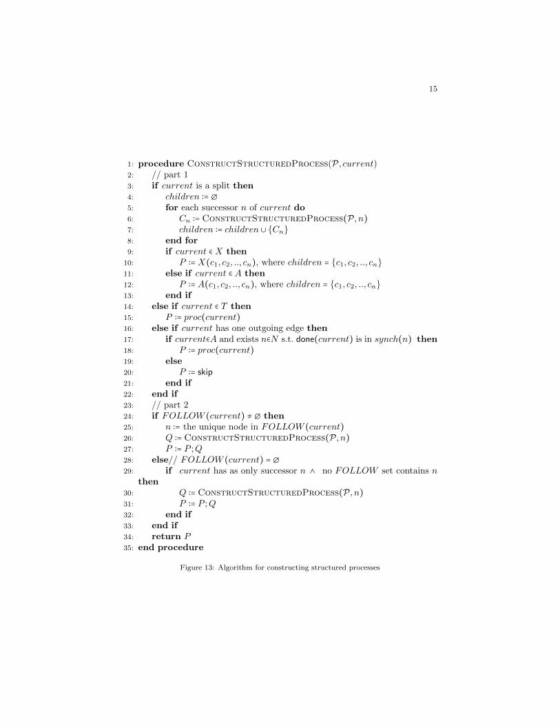
The algorithm is listed in Figure 13. It takes as input a process flow graphP = (N,T,A,X, start, end,E, synch), and the node current that is to be pro-cessed. The algorithm returns a sequential block that starts with current. Theinitial call is ConstructStructuredProcess(P, start).

The algorithm has two main parts.

– In Part 1 (l. 3-22), the node current is processed by creating a sequentialblock P containing current and all its indirect successors that are not inFOLLOW (current). By definition, these indirect successors are on thepath from current to the unique node in FOLLOW (current).

– In Part 2 (l. 24-33), the nodes in FOLLOW (current) are processed by re-cursively calling ConstructStructuredProcess; the resulting blockis appended to P . If FOLLOW (current) = ∅ then under certain con-ditions (see l.29) the successor of current is processed, in which case theprocess block starting with current is duplicated in the structured process.Finally (l. 34), P is returned as the structured composition for current.

We now explain these parts in more detail. We illustrate the different partsby Examples 7-11, which form a running example that refers to the process inFigure 1 after preprocessing.

Part 1. The algorithm first processes the node current, which creates a sequen-tial block P containing current and all its (in)direct successors that are not inFOLLOW (current) There are three cases.

15

1: procedure ConstructStructuredProcess(P, current)2: // part 13: if current is a split then4: children ∶= ∅5: for each successor n of current do6: Cn ∶= ConstructStructuredProcess(P, n)7: children ∶= children ∪ {Cn}

8: end for9: if current ∈X then

10: P ∶=X(c1, c2, .., cn), where children = {c1, c2, .., cn}11: else if current ∈ A then12: P ∶= A(c1, c2, .., cn), where children = {c1, c2, .., cn}13: end if14: else if current ∈ T then15: P ∶= proc(current)16: else if current has one outgoing edge then17: if current∈A and exists n∈N s.t. done(current) is in synch(n) then18: P ∶= proc(current)19: else20: P ∶= skip21: end if22: end if23: // part 224: if FOLLOW (current) ≠ ∅ then25: n ∶= the unique node in FOLLOW (current)26: Q ∶= ConstructStructuredProcess(P, n)27: P ∶= P ;Q28: else// FOLLOW (current) = ∅29: if current has as only successor n ∧ no FOLLOW set contains n

then30: Q ∶= ConstructStructuredProcess(P, n)31: P ∶= P ;Q32: end if33: end if34: return P35: end procedure

Figure 13: Algorithm for constructing structured processes

16

– If current is a split node (l. 3, then each successor n of current is pro-cessed in a for-loop (l. 5). By the first preprocessing step, n is not a join.Therefore, n is a task or a split or a loop node. By definition node n doesnot appear in the FOLLOW set of any node, so n is not processed in thesecond part of the algorithm. First, algorithm ConstructStructured-Process is recursively called for n and returns a block Cn that containsn (l. 6). Finally, block Cn is added to the set children (l. 7). After thefor-loop has finished, all child blocks have been computed and a compositeblock P containing all child blocks in children is created. The type of Pdepends upon the connector type of current (l. 9 and l. 11).

Example 7. If current = A1, then the algorithm creates two child blocks,one starting with Inspect vehicle, the other with Accept claim; see Figure 2.

– If current is a task (l. 14), then a process flow graph only containingcurrent is created, denoted proc(current) (l. 15). Unlike the previous twocases, the successor nodes of current are now not processed immediately.Since current is not a split or a loop node, the unique successor node xof current is in some set FOLLOW (n), where n is a node. If current isthe only predecessor of x, then x ∈ FOLLOW (current), so current = n.Otherwise, x is a join node and n is a split node. In both cases, node x isprocessed in l. 24-33 if node n is processed as current.

Example 8. If current = Inspect vehicle, then the algorithm creates ablock only containing task Inspect vehicle. The unique successor of Inspectvehicle is AND split A2 which is processed at l. 24; see Example 10.

– If current has one outgoing edge but is not a task (l. 16), then currentis a join. If current ∈ A and current is referenced in a synchronizationcondition of a node n ∈ N , i.e. synch(n) contains done(current), thenblock P has to contain a task current. Therefore in line 18 a new dummytask current is created using proc(current). Otherwise, an empty block(skip) is created. The empty block is removed if it is concatenated withanother block, so skip;Q is equivalent to Q.

Example 9. If current = X2, then the algorithm creates an empty blockskip. If current = A3 then the algorithm creates at line 18 a block only con-taining dummy task A3, since A3 is an AND split and the synchronizationcondition of File report contains done(A3) (cf. Example 6).

Part 2. Next, the algorithm processes set FOLLOW (current). There are twooptions.

– If FOLLOW (current) ≠ ∅ (l. 24), then by definition there is a uniquenode n such that FOLLOW (current) = {n}. Variable n gets assignedthis node n. The algorithm is invoked for node n (l. 26), and the returnedblock is appended to the block P created for current (l. 27).

17

Example 10. If current = X2, then n = A3. The block P created for X2 isskip (cf. Example 9). The block Q created for A3 is A3;Send decision. Thenew block P at line 27 becomes A3;Send decision, since the empty blockskip created for X2 is removed when concatenated with the block createdfor A3.

For current = Inspect vehicle, node n = A2. The block Q created for A2 isA(A3;Send decision , Approve payment;Pay). The next Example 11 explainshow block Approve payment;Pay is constructed.

– If FOLLOW (current) = ∅ (l. 28), then if current has a single successorn for which is there is no node x such that n ∈ FOLLOW (x), then nis processed next by invoking the algorithm for n (l. 30). Since currenthas only one successor n yet n ∉ FOLLOW (current), n has to be a join.By property P4, n ∈ X so n is a XOR join. The block created for n isappended to P .

Example 11. For current = Approve payment, set FOLLOW (Approvepayment) = ∅ and its unique successor X3 is not contained in any FOLLOWset (cf. Table 1). The block Q created for X3 only contains Pay, thereforeP becomes Approve payment;Pay.

Finally, block P is returned (l. 34).

Example 12. Applying the algorithm to the process flow graph in Figure 1 re-sults in the semi-structured process flow graph visualized in Figure 2. Dummytask (A3) is needed to specify the cross-synchronization between the parallelbranches using condition [done(A3)]. Example 9 explains how the algorithmgenerates dummy task A3.

The part of the process flow graph between X2, X3 and A6 is duplicated bythe algorithm. Node X2 gets processed twice as a result of processing splits A2and A5 (recursive invocation at l. 6). Node X2 is not processed at l. 30 when A2(or A5) is current: although FOLLOW (A2) = ∅, node A2 (A5) has more thanone successor.

Node X3 is also processed twice. The first processing of X3 starts at l. 6when A5 is current. The second one starts if Approve payment is processed ascurrent, explained in Example 11. Since X3 is processed twice, two duplicateblocks containing Pay have been created for the semi-structured process in Fig-ure 2. Without introducing duplicates, no structured process equivalent existsfor the process flow graph, unless auxiliary variables are used [11]. ◻

We prove the correctness of the algorithm in two propositions, the proofs ofwhich are in Appendix B. First we show that every node in an input processflow graph gets processed by the algorithm.

18

Proposition 1. Let P be a process flow graph that is an input parameter to theinitial invocation of algorithm ConstructStructuredProcess. Each noden of P is processed at least once by ConstructStructuredProcess, i.e.,there is an invocation with current = n.

The algorithm can process a node multiple times, subject to a maximumbounded of the number of its incoming edges. For instance, X2 in Figure 1 isprocessed two times because it has two incoming edges, from A1 and A2. Eachprocessing of a node n results in a separate block in the structured process (cf.line 6). The algorithm therefore runs in time linear to the number of nodes andedges of the input process flow graph. However, the worst-case time complex-ity of the whole approach is slightly higher, since computing dominators takesalmost linear time [27], but still polynomial.

Next, the main proposition shows that the algorithm converts a processflow graph satisfying properties P1-P4 into an equivalent structured processes,neither reducing nor adding behavior. Note that properties P1-P4 hold for everypreprocessed process flow graph.

Proposition 2. If a process flow graph P satisfies properties P1-P4 and iscorrect, then P is equivalent to the structured process returned by Construct-StructuredProcess for P.

Next, we discuss the validation of the approach.

6. Evaluation

To evaluate the feasibility of the method, we have implemented the prepro-cessing rules and the algorithm, including its extensions in Appendix A, in Struc-tXPDL, a Java-based tool which reads process models in XPDL format [28], anXML standard for exchanging process models. To compute dominators, we usethe polynomial time algorithm developed by Lengauer and Tarjan [27].

To evaluate the utility of the method, we compare it with the approachdeveloped by Polyvyanyy et al. [18]. We perform the comparison by applyingthe method, using the tool StructXPDL, to eleven correct benchmark examplesdeveloped for the BPStruct tool [29] — which implements the approach devel-oped by Polyvyanyy et al. [18] — and comparing the outcomes. The modelsare acyclic and contain mixtures of AND and XOR splits and joins. A com-panion online appendix lists the examples as well as the outputs generated bythe tool. Table 3 compares the performance of BPStruct and StructXPDL onthese benchmark examples. Several interesting conclusions can be drawn fromthe comparison.

First, for the seven models that BPStruct can structure, StructXPDL alsooutputs a structured process model. Moreover, the structured process modelsthat are constructed by BPStruct and StructXPDL for each of these sevenmodels are identical, which indicates the StructXPDL method is sound for theseexamples. In addition, StructXPDL outputs semi-structured process models for

19

Table 3: Comparing BPStruct and StructXPDL on benchmark examples

Inputmodel

BPStructoutput

StructXPDLoutput

identical? identical afterextra prepro-cessing?

7817 structured structured yes7818 structured structured yes7819 – semi-structured –7820 structured semi-structured no yes7821 – semi-structured –7822 structured structured no yes7823 – semi-structured –7824 structured structured no yes7825* structured structured yes7826 – semi-structured –7827 structured structured no yes*Loop modified into repeat-until structure

the four models that BPStruct cannot structure. All these four structured modelscontain cross-synchronization and are constructed using the algorithm detailedin Section 5, which clearly shows the benefit of the method. For instance,Figure 14(a) shows the original model 7826, which does not have a structuredequivalent, so BPStruct does not generate an output model. However, ouralgorithm constructs after preprocessing the semi-structured process shown inFigure 14(c). Notice that for a reader Figure 14(c) is much more understandablethan Figure 14(a). In the figure, X is the label of the XOR node that is thesource of the synchronization edge in Figure 14(b). Node X is included byprocessing line 18 in Figure 13. Semantically, done(X) is true when node Xhas been activated by any of its incoming edges. The process can be simplifiedfurther by replacing the parallel subprocess containing X and skip with theprocess containing a single task X.

Second, for some models StructXPDL outputs a structured process that isdifferent from the structured process created by BPStruct. In all these cases, theinput model contains a subgraph consisting of j splits and n joins for n, j ≥ 2,where for every split-join pair, there is an edge from the split to the join, andevery edge entering the subgraph enters a split while every edge leaving thesubgraph exits a join. To illustrate this subgraph structure, Figure 15(a) showsmodel 7827, where j = n = 2. Since the splits have type AND and the joins areXOR, the algorithm duplicates c and d; it returns the structured process shownin Figure 15(b).

To remove duplication, we experimented with an additional preprocessingrule, which replaces the subgraph with one join and subsequent split; Fig-ure 15(c) shows the process flow graph of (a) after additional preprocessing.If StructXPDL with the additional preprocessing rule is applied to model 7827,it produces the structured process shown in Figure 15(c), so the output is then

20

(a) Input model

X

[done(X)]

(b) Input model after preprocessing

[done(X)]

(c) Generated semi-structured process model

Figure 14: Preprocessing of benchmark model 7826

21

identical to the output model produced by BPStruct. More generally, withthis additional preprocessing rule StructXPDL and BPStruct produce identicalmodels for all input models listed in Table 3.

We also applied the tool to another unstructured process which containsseveral cross-synchronizations between parallel branches [30]. While the modelcannot be structured with BPStruct, StructXPDL outputs a semi-structuredprocess model.

From the comparison based on these examples, we conclude that the pro-posed method outputs (semi-)structured process models for all (correct) inputmodels. The BPStruct tool is able to convert only some of the process modelsto equivalent structured models, because it restricts itself to structured models.Since cross-synchronization between parallel branches occurs quite frequently,this is a useful improvement over the current state of the art implemented in theBPStruct tool. Next, the comparison shows that the algorithm does not alwaysreturn minimal models. But for all these cases, if an additional preprocessingrule is used, the algorithm does return a minimal model that is equivalent tothe models created by BPStruct.

7. Related Work

Early works addressing structured process models are [10, 11], in which theclass of structured process models is defined and their expressiveness is ana-lyzed. Informal transformations are proposed to convert unstructured processpatterns to structured patterns, extending existing translation patterns usedto structure sequential programs. However, no complete overall conversion ap-proach is proposed in these early works.

Ouyang et al. [17] focus on recognizing structured patterns in unstructuredprocess models and mapping them to structured BPEL fragments, but they donot address how an unstructured process model can be structured. For example,the unstructured process model in Figure 1 cannot be structured using theapproach of Ouyang et al.

Other related work [31] proposes to decompose a process flow graph intoSESE regions, based on transformation rules that build the regions incremen-tally. A SESE region has a unique entry and a unique exit node. Our approachdoes not use SESE regions; instead, the complete process flow graph is processed.Citation [31] also sketches how each atomic SESE region (not containing anyother SESE region) can be converted into a structured process but does notprovide a complete specification for that conversion. In particular, it is notdiscussed in what circumstances duplications are required. The algorithm inSection 5 defines precisely when duplications of tasks and blocks are made.

The work most closely related to ours is by Polyvyanyy et al. [18], whooutline a method for structuring acyclic process models; the method has beenimplemented in the BPStruct tool [29], discussed in Section 6. In the BPStructmethod, first a process model is translated into Petri nets and decomposed intoa refined process structure tree (RPST) consisting of SESE regions. Next, each

22

(a) Input model

(b) Generated structured model for (a)

(c) Generated structured model for (a) after additional preprocessing

Figure 15: Additional preprocessing of benchmark model 7827.

23

Table 4: A comparison of our approach with the BPStruct approach [18]

Aspect BPStruct approach Our approach

Language Petri nets Process flow graphsBasis for structuring Petri-net unfoldings, Dominators

ordering relations graphsOutput Structured process models Semi-structured, structured

process modelsDuplicate tasks Allowed AllowedOptional tasks Not allowed AllowedLoops Not allowed SESE loops allowedTime complexity Exponential Polynomial

region is unfolded into an equivalent region that contains no XOR joins. Theunfolding may lead to duplication of tasks. A graph containing ordering rela-tions between tasks is derived from the unfolding. The ordering relations graphcan be translated (sometimes) into a structured region. The complete approachcombines techniques from different areas, in particular Petri net unfoldings andordering relations graphs. In a follow-up paper, Polyvyanyy et al. [32] refinethe approach to obtain maximally structured process models, i.e., models thatcontain as many structured subprocesses as possible.

There are several differences between BPStruct and our work. The worst-case time complexity of BPStruct is exponential, though the authors argue thatthe average complexity is much lower in practice. In contrast, our approachruns in polynomial time. Another difference is that they do not consider semi-structured process models which can be generated with the algorithm proposedin this paper. Finally, for process models that contain optional tasks the order-ing graph does not capture the process behavior accurately since the orderinggraph will treat all tasks as mandatory. For instance, a process in which firsttask A is done, then either B or nothing, and finally C, translates using theordering graph into a structured process in which A, B, C are done in sequence.Like the extended BPStruct approach [32], our approach constructs maximallystructured process models. A summary of the comparison is shown in Table 4.

Finally, there is a large body of work on structuring control flow graphs(see [33] for an overview), but these are sequential while the process flow graphsunderlying process models contain parallelism. There are a few papers thatanalyze concurrent flow graphs [34, 35]. However, these flow graphs are de-rived from programs that contain structured parallelism, i.e. a block containingparallelism is demarcated with a cobegin and a coend statement, and differentblocks containing parallelism are either disjoint or properly nested. In con-trast, the process flow graphs in this paper can contain arbitrary, unstructuredparallelism, for instance the example presented in Figure 1.

The contribution of this paper is the formal definition of a polynomial timealgorithm for converting correct, unstructured process models into equivalent(semi-)structured ones.

24

8. Conclusion

We have presented an algorithm that converts any correct, unstructuredprocess flow graph into a (semi-)structured process. Such processes are easier tounderstand and implement than unstructured ones. Process flow graphs extendcontrol flow graphs with unstructured but bounded concurrency and underlyprocess model notations such as Petri nets [36], UML activity diagrams [16]and BPMN [15]. Semi-structured process models are structured processes thatcontain concurrency and cross-synchronization between parallel branches andunderly notations such as BPEL [3] and OWL-S [4]. The algorithm enables asmooth translation from user requirements on business processes documentedin process flow graphs into deployable process models that support the businessprocesses. One drawback is that the algorithm sometimes generates duplicateparts when a structured model without duplicates may also exist, so the modelsare not always minimal. For the examples we checked, the duplicates can beremoved using one additional preprocessing rule.

Further work includes adding more pre- and post-processing rules to ourprototype. It would also help to extend the translation to other operators thansequence, choice, and parallelism. For instance, BPMN uses the notion of an ORsplit: a connector in which the number of outgoing edges taken is determinedat run-time when the connector is visited. Implementing this approach in anexisting workflow system is also an interesting exercise.

References

[1] M. Dumas, M. L. Rosa, J. Mendling, H. A. Reijers, Fundamentals of Busi-ness Process Management, Springer, 2013.

[2] M. Weske, Business Process Management - Concepts, Languages, Archi-tectures, 2nd Edition, Springer, 2012.

[3] A. Alves, A. Arkin, S. Askary, C. Barreto, B. Bloch, F. Curbera,M. Ford, Y. Goland, A. Guzar, N. Kartha, C. K. Liu, R. Kha-laf, D. Koenig, M. Marin, V. Mehta, S. Thatte, D. Rijn,P. Yendluri, A. Yiu, Web services business process executionlanguage version 2.0 (OASIS standard), WS-BPEL TC OASIS,http://docs.oasis-open.org/wsbpel/2.0/wsbpel-v2.0.html (2007).

[4] D. Martin (editor), M. Burstein, J. Hobbs, O. Lassila, D. McDermott,S. McIlraith, S. Narayanan, M. Paolucci, B. Parsia, T. Payne, E. Sirin,N. Srinivasan, K. Sycara, Owl-s: Semantic markup for web services,http://www.w3.org/Submission/OWL-S/ (2004).

[5] D.-R. Liu, M. Shen, Workflow modeling for virtual processes: an order-preserving process-view approach, Inf. Syst 28 (6) (2003) 505–532.

[6] R. Eshuis, P. Grefen, Constructing customized process views, Data andKnowledge Engineering 64 (2) (2008) 419–438.

25

[7] J. Bae, H. Bae, S.-H. Kang, Y. Kim, Automatic control of workflow pro-cesses using eca rules, IEEE Trans. Knowl. Data Eng. 16 (8) (2004) 1010–1023.

[8] M. Reichert, P. Dadam, ADEPTflex: Supporting Dynamic Changes ofWorkflow without Loosing Control, Journal of Intelligent Information Sys-tems 10 (2) (1998) 93–129.

[9] C. Bohm, G. Jacopini, Flow diagrams, turing machines and languages withonly two formation rules, Commun. ACM 9 (5) (1966) 366–371.

[10] B. Kiepuszewski, A. ter Hofstede, C. Bussler, On structured workflow mod-elling, in: B. Wangler, L. Bergman (Eds.), Proc. CAiSE ’00, Springer, 2000,pp. 431–445.

[11] R. Liu, A. Kumar, An analysis and taxonomy of unstructured workflows.,in: W. van der Aalst, B. Benatallah, F. Casati, F. Curbera (Eds.), Proc.3rd Conference on Business Process Management (BPM 2005), Vol. 3649of Lecture Notes in Computer Science, 2005, pp. 268–284.

[12] M. Dumas, M. L. Rosa, J. Mendling, R. Maesalu, H. A. Reijers, N. Seme-nenko, Understanding business process models: The costs and benefits ofstructuredness, in: J. Ralyte, X. Franch, S. Brinkkemper, S. Wrycza (Eds.),CAiSE, Vol. 7328 of Lecture Notes in Computer Science, Springer, 2012,pp. 31–46.

[13] R. Laue, J. Mendling, Structuredness and its significance for correctness ofprocess models, Inf. Syst. E-Business Management 8 (3) (2010) 287–307.

[14] J. Mendling, H. A. Reijers, W. M. P. van der Aalst, Seven process modelingguidelines (7PMG), Information & Software Technology 52 (2) (2010) 127–136.

[15] BPMN Task Force, Business Process Model and Notation (BPMN) Ver-sion 2.0, Object Management Group, 2011, oMG Document Numberformal/2011-01-03.

[16] UML Revision Taskforce, UML 2.3 Superstructure Specification, ObjectManagement Group, 2010, oMG Document Number formal/2010-05-05.

[17] C. Ouyang, M. Dumas, A. ter Hofstede, W. van der Aalst, Pattern-basedtranslation of BPMN process models to BPEL web services, InternationalJournal of Web Services Research 5 (1) (2008) 42–61.

[18] A. Polyvyanyy, L. Garcıa-Banuelos, M. Dumas, Structuring acyclic processmodels, Inf. Syst. 37 (6) (2012) 518–538, prelimary version appeared inProc. BPM 2010.

[19] A. Aho, R. Sethi, J. Ullman, Compilers: Principles, Techniques, and Tools,Addison Wesley, 1986.

26

[20] J. Koehler, R. Hauser, Untangling unstructured cyclic flows - a solu-tion based on continuations., in: R. Meersman, Z. Tari (Eds.), Proc.CoopIS/DOA/ODBASE 2004, Lecture Notes in Computer Science 3290,Springer, 2004, pp. 121–138.

[21] W. Zhao, R. Hauser, K. Bhattacharya, B. Bryant, F. Cao, Compiling busi-ness processes: untangling unstructured loops in irreducible flow graphs,Int. Journal of Web and Grid Services 2 (2006) 68–91.

[22] Y. Choi, P. Kongsuwan, C. M. Joo, J. L. Zhao, Stepwise structural verifi-cation of cyclic workflow models with acyclic decomposition and reductionof loops, Data Knowl. Eng. 95 (2015) 39–65.

[23] R. Diestel, Graph Theory, Vol. 173 of Graduate Texts in Mathematics,Springer, 2005.

[24] W. Sadiq, M. Orlowska, Analyzing process models using graph reductiontechniques, Information Systems 25 (2) (2000) 117–134.

[25] R. Eshuis, A. Kumar, An integer programming based approach for verifica-tion and diagnosis of workflows, Data Knowl. Eng. 69 (8) (2010) 816–835.

[26] B. Baker, An algorithm for structuring flowgraphs, Journal of the ACM24 (1) (1977) 98–120.

[27] T. Lengauer, R. Tarjan, A fast algorithm for finding dominators in a flow-graph, ACM Transactions on Programming Languages and Systems 1 (1)(1979) 121–141.

[28] Workflow Management Coalition, Workflow process definition interface –XML process definition language, Tech. Rep. WFMC-TC-1025, WorkflowManagement Coalition (2002).

[29] BPstruct team, http://bpt.hpi.uni-potsdam.de/Public/BPStruct

(2012).

[30] H. Lin, Z. Zhao, H. Li, Z. Chen, A novel graph reduction algorithm toidentify structural conflicts, in: Proc. of the 35th Ann. Hawaii InternationalConference on System Science (HICSS-35), IEEE Computer Society Press,2002.

[31] R. Hauser, M. Friess, J. M. Kuster, J. Vanhatalo, An incremental approachto the analysis and transformation of workflows using region trees, IEEETransactions on Systems, Man, and Cybernetics, Part C 38 (3) (2008)347–359.

[32] A. Polyvyanyy, L. Garcıa-Banuelos, D. Fahland, M. Weske, Maximal struc-turing of acyclic process models, Comput. J. 57 (1) (2014) 12–35.

[33] F. Zhang, E. H. D’Hollander, Using hammock graphs to structure pro-grams, IEEE Trans. Software Eng. 30 (4) (2004) 231–245.

27

X1

X2 X3

X4

Figure A.16: Process flow graph with loop

[34] J. Krinke, Static slicing of threaded programs, in: T. Ball, F. Tip, A. M.Berman (Eds.), Proc. SIGPLAN/SIGSOFT Workshop on Program Analy-sis For Software Tools and Engineering, PASTE ’98, ACM, 1998, pp. 35–42.

[35] J. Lee, S. P. Midkiff, D. A. Padua, A constant propagation algorithm forexplicitly parallel programs, International Journal of Parallel Programming26 (5) (1998) 563–589.

[36] T. Murata, Petri nets: Properties, analysis, and applications, Proc. of theIEEE 77 (4) (1989) 541–580.

[37] R. Eshuis, P. Grefen, Composing services into structured processes, Int. J.Cooperative Inf. Syst. 18 (2) (2009) 309–337.

Appendix A. Loops

As explained in Section 1, the main text considers acyclic process flow graphsto simplify the exposition. This Appendix shows how to extend the algorithmof Section 5 to deal with process flow graphs with structured loops, in whicheach loop has a single entry and a single exit point. Other papers [37, 20, 21]already discuss techniques to turn a process model with unstructured loops intoan equivalent process model in which each loop has a single entry and a singleexit point. These techniques are complementary to our approach and can beeasily integrated.

Appendix A.1. Definitions

We introduce additional definitions to deal with loops. A back edge is anedge (x, y) ∈ E in the process flow graph such that y dominates x [19], thusevery path from start to x passes through y. Intuitively, a back edge (x, y)closes a cycle that is started at y. An edge that is not a back edge is called aforward edge.

Example 13. Figure 1 only has forward edges. Figure A.16 has one back edge:(X3,X2). Note that node X2 dominates node X3.

A node l that is the target of some back edge is called a loop node. Themodified algorithm defined below creates a repeat-until statement for l. In acorrect process flow graph, each loop node is a XOR node that has multiple

28

incoming edges. To simplify the presentation, we require that each loop nodehas a single outgoing forward edge, so each loop node is a XOR merge. Ifa node violates this constraint because the loop node has multiple outgoingforward edges, the graph can be easily repaired by splitting the loop node in aXOR merge and subsequent XOR split.

For a non-loop node n, its loop head, denoted HEAD(n), is the most nestedloop node l such that l strictly dominates n (so there is a path from l to n) andthere is a reverse path from n to l via a back edge (x, l), where x ∈ N . In theconstructed semi-structured process, n is contained in the body of the repeat-until statement constructed for HEAD(n). If n is not contained in a loop, nodeHEAD(n) is undefined. For convenience, if HEAD(n1) and HEAD(n2) areundefined, then HEAD(n1) = HEAD(n2) by definition. Note that for a loopnode l, HEAD(l) is either another loop node or undefined.

Example 14. For Figure A.16, X2 is header for nodes Repair damage, Checkrepair, and X3. All the other nodes, including X2 itself, have no header. In par-ticular, X2 is not header for Determine bill since there is no path from Determinebill to X2 via X3.

For a loop node l, so some back edge enters l, define

FOLLOW (l) = { n ∣ HEAD(n) =HEAD(l) ∧ HEAD(IDOM(n)) = l }.

So n ∈ FOLLOW (l) if and only if n and l have the same loop header and theimmediate dominator of n is in a loop headed by l. In that case, we call nodeIDOM(n) a loop-exit for the loop started at l. By definition, IDOM(n) is asplit node. We require that IDOM(n) is a XOR node; if IDOM(n) were anAND node, each execution would remain in the loop after reaching IDOM(n)and in parallel start a new copy of the subprocess started at l. This results inunbounded many instantiations of the subprocess, which cannot be expressedin structured process models.

Next, we have to redefine the existing definition of FOLLOW . For everyother node n1 ∈ N , so n1 is not a loop node, define

FOLLOW (n1) = { n2 ∣ n1 = IDOM(n2) ∧ n2 = IPDOM(n1)

∧ HEAD(n1) =HEAD(n2) }.

So for a non-loop node n, each node y in the FOLLOW set of n must have thesame loop header as n.

Example 15. For Figure A.16, for example FOLLOW (X2) = {Determine bill},FOLLOW (Repair damage) = {Check repair}, FOLLOW (Check repair) = {X3},and FOLLOW (X3) = ∅. Furthermore, X3 is a loop-exit for the loop started atX2.

In the sequel we only consider process flow graphs in which each loop nodel has exactly one node in its FOLLOW set. This means that in addition to theproperties listed in Table 2, we have new property:

29

P5 For each loop node l, ∣FOLLOW (l)∣ = 1.

Furthermore, to simplify the presentation, we only consider process flowgraphs with repeat-until loops, which have a single exit point. That is, for aloop node l there is exactly one exit point x and x is a XOR split that has anoutgoing backedge to l, so (x, l) ∈ E. For structuring loops with multiple exits,the approaches outlined in [20, 21] can be used.

To encode loops in structured processes, we extend the notation from Sec-tion 3 with construct repeat P until grd, which specifies that block P is executeduntil condition grd holds.

Appendix A.2. Modification of Algorithm for handling loops

We add the following else-if clause after line 13 in Figure 13:

else if current is a loop node with FOLLOW (current) = {n} thens ∶= the unique successor of currentPx ∶= ConstructStructuredProcess(P, x)x ∶= the loop-exit of currentP ∶= repeat Ps until condition on edge (x,n)

end if

If current is a loop node (l. 1), then by P5 there is a unique node sthat is the successor of current. For s, a block Ps is created by invokingConstructStructuredProcess(P, s) (l. 3). By assumption the loop hasa single exit point x, which is a split. There is an edge from x to a uniquenode n outside the loop such that FOLLOW (current) = {n}. If node x isreached and the condition annotated on (x,n) is true, the loop is exited. Sincewe focus on repeat-until loops, split x has no outgoing forward edges that targetnodes inside the loop. Therefore, x closes the block started at s and the blockrepeat Ps until condition on (x,n) represents the entire loop.

Appendix B. Proofs of Section 5

This Appendix contains the proofs of the propositions defined in Section 5.We first prove new Proposition 3, used in the other proofs, that states thatproperties P1-P5 (cf. Table 2) hold for preprocessed process flow graphs.

Proposition 3. After preprocessing each process flow graph P =

(N,T,A,X, start, end,E, synch) satisfies properties P1-P5.

Proof. The first two properties hold for any process flow graph. Property P3holds after refactoring transitive edges. Property P4 holds after synchroniza-tion links have been removed from the set E of edges in a process flow graph.Property P5 follows from our definition of loops. ◻

We now prove the propositions stated in Section 5.Proof of Proposition 1. Let n be an arbitrary node of P that is processedby the algorithm ConstructStructuredProcess as current. We show thateach successor node of current is processed too. Since the process flow graph is

30

connected, and in the initial invocation the start node is processed as current,this proves the claim.

There are two cases:

1. If current is a split, then each successor n is processed directly (l. 6).

2. If current is a task or an AND/XOR node with one outgoing edge, thencurrent has by constraint a unique successor x. In that case, by P2 either(i) FOLLOW (current) = {x} or (ii) FOLLOW (current) = ∅. (i) ByP1, there is no other node n′ such that x ∈ FOLLOW (n′). Node x istherefore processed exactly once at l. 26. (ii) There are two subcases forx. (a) Either there is a split s such that FOLLOW (s) = {x}. Thenx is processed when s is processed as current. (b) Or x is not in theFOLLOW set of any node. Then by P4, x is not in A, therefore x ∈ X.Since x is the only successor of current, node x gets processed at l. 30. ◻

Proof of Proposition 2. (Sketch.) By preprocessing link edges are re-moved from P. It is straightforward to check that the synchronization con-ditions created by Algorithm RemoveCrossSynchronization preserve thesynchronization constraints expressed by the removed link edges. We now focuson the correctness of algorithm ConstructStructuredProcess.

We prove the proposition for any process flow graph P obtained after prepro-cessing. We consider the different blocks (parts) of the semi-structured processflow graph created by ConstructStructuredProcess for P. Each block hasa single entry and a single exit node such that each edge from a node outside theblock that targets a node inside the block must target the entry node, and eachedge from a node inside the block to an outside node must leave the exit node.

Let P = (N,T,A,X, start, end,E, synch) be a process flow graph after pre-processing and let n ∈ N be a node of P. The block created by Construct-StructuredProcess when processsing n as current corresponds to a sub-graph of P. We first identify this subgraph, and then show that each subgraphis equivalent to its corresponding block.

First, observe that if ConstructStructuredProcess(P, n) is invoked,then processing n can result in a recursive invocation of ConstructStruc-turedProcess in which an (indirect) successor of n is processed as current andalso included in the block for n. For a node n ∈ N , we now define a set range(n)containing all nodes processed as current by the algorithm when the initial invo-cation is ConstructStructuredProcess(P, n). Formally, range(n) is thesmallest non-empty set of nodes S ⊆ N satisfying

– n ∈ S;

– if x is a forward successor of some node in S, and either:

– x is not in the FOLLOW set of any node in N , or

– x is in the FOLLOW set of a node y ∈ S,

then x ∈ S.

31

The construction of range(n) stops when one or more nodes y are reached suchthat y ∈ FOLLOW (z) for some node z ∉ range(n). Such a node y is processedwhen ConstructStructuredProcess(P, z) is invoked, and is therefore notcontained in the block created for n.

For each node n ∈ N , we define the subgraph S that is induced by range(n).Formally, the subgraph S of P induced by range(n) is a tuple (T ′,A′,X ′, start′,E′, synch′), where:

– T ′ = T ∩ range(n) is a set of tasks,

– A′ = A ∩ range(n) is a set of AND nodes,

– X ′ =X ∩ range(n) is a set of XOR nodes,

– start′ = n is the unique start node,

– E′ = E ∩ (range(n) × range(n)) is the control flow (transition) relation,

– synch′ = synch ∩ (A→ BExp).

The subgraph S typically has no unique end node. For instance, for A1 andA2 in Figure 1 after preprocessing, so edge (A3,A4) has been removed, we haverange(A2) = range(A5) = {X2,A3,Send decision,Approve payment,X3,Pay}, sothe range contains end nodes Send decision and Pay.

To prove the proposition, we now prove the following claim: for each node n ∈

N , the subgraph S induced by n is equivalent to the structured process returnedby ConstructStructuredProcess(P, n). The proof is by induction on thenesting level of the induced subgraphs. A subgraph induced by node n is nestedinside a subgraph induced by node n′ if range(n) ⊂ range(n′). The base case,where the subgraph induced by n does not contain any other subgraph, i.e.range(n) = {n}, is trivially true.

For the induction case: we prove the claim for a subgraph induced by node n,assuming the claim holds for all subgraphs nested inside the subgraph inducedby n. We consider the different cases for n.

1. n is an AND or XOR split. If the algorithm ConstructStructured-Process is invoked when n is current, an AND or XOR block is created (l. 3and further), depending on the connector type of n. The block created for eachsuccessor x of n is a child of this block. By properties P3 and P4, x is not anAND join, so the block for x does not need synchronization with another blockbefore it can start. By the induction hypothesis, the block created for x at l. 5is equivalent to the subgraph induced by x.

The block opened for n can be closed in two different ways. If FOLLOW (n) ={y} then y is by definition a join that closes the block P started at n andy ∈ range(n). By P3, y is not an immediate successor of n, so no block fory has been created at line 5. Therefore for y only one block Q is created, atline 26. By the induction hypothesis, Q is equivalent to the subgraph inducedby y. Consequently, P ;Q is equivalent to the subgraph induced by n.

If FOLLOW (n) = ∅ then the block created for n is P . In particular, Pdoes not contain the post dominator IPDOM(n) of n. By construction, set

32

range(n) does not include IPDOM(n). Consequently, P is equivalent to thesubgraph induced by n.

2. n is a loop node. (Defined in Appendix A.) By P5, n has a uniquesuccessor s. Next, there is a unique exit point x and FOLLOW (n) = {e} with(x, e) ∈ E. By the induction hypothesis, the subgraph started at s is equiva-lent to the block Ps returned by recursively calling the algorithm Construct-StructuredProcess at l. 3. Since the loop has by constraint only one exitpoint, node x has no outgoing forward edges that target nodes in the loop headedby n. The block Ps is therefore closed by x and exited when the condition onedge (x, e) is true. Therefore block P = repeat Ps until condition on edge (x,n)(l. 5) is equivalent to the first part of subgraph induced by n, which ends at e.Next, a block Pe is created by recursively invoking the algorithm Construct-StructuredProcess at l. 26 and Pe is appended to P . By the inductionhypothesis, block Pe is equivalent to the subgraph induced by e. The resultingblock P is therefore equivalent to the entire subgraph induced by n.

3. n is a task, or an AND or XOR node with one outgoing edge. If thealgorithm ConstructStructuredProcess is invoked when n is current, ablock n is created if n is a task (l. 15) and a block skip is created if n is anAND/XOR node with one outgoing edge (l. 20).

Next, let y be the single successor of n in P. There are two subcases.

3.1 FOLLOW (n) = {y}. By the induction hypothesis, for the subgraph in-duced by y an equivalent block Q is created, by recursively calling thealgorithm ConstructStructuredProcess (l. 26). The block n;Q orskip;Q is therefore equivalent to the subgraph induced by n, dependingon whether n is a task or an AND/XOR node.

3.2 FOLLOW (n) = ∅. Since y ∉ FOLLOW (n), y is a join node. There aretwo further subcases.

3.2.1 No FOLLOW set contains y. By the induction hypothesis, forthe subgraph induced by y an equivalent block Q is created, byrecursively calling the algorithm ConstructStructuredProcess(l. 30). By property P4 y is not an AND join, so y is a XOR join. Asthe process flow graph is correct, there is no lack of synchronizationat y, and P ;Q is equivalent to the subgraph induced by n.

3.2.2 y ∈ FOLLOW (z) for some node z ≠ n. In that case, the condition ofthe if-statement at l. 29 is false, and the complete block P createdfor n is either P = n, if n is task, or P = skip if n is an AND/XORjoin. By construction y /∈ range(n), so P is the block equivalent tothe subgraph induced by n.

Thus, by induction and case by case enumeration, we have shown that theproposition is true. ◻