convergence time improvement of precise point positioning · convergence time improvement of...

TS04J - Geodetic Applications in Various Situations, 5249 Mohamed Elsobeiey and Ahmed El-Rabbany Convergence Time Improvement of Precise Point Positioning FIG Working Week 2011 Bridging the Gap between Cultures Marrakech, Morocco, 18-22 May 2011

1/15

Convergence Time Improvement of Precise Point Positioning

Mohamed Elsobeiey and Ahmed El-Rabbany, Canada

Key words: GPS, Precise Point Positioning, satellite orbit, clock corrections, ionosphere

SUMMARY Presently, precise point positioning (PPP) requires about 30 minutes or more to achieve centimetre- to decimetre-level accuracy. This relatively long convergence time is a result of the un-modelled GPS residual errors. A major residual error component, which affects the convergence of PPP solution, is higher-order ionospheric delay. In this paper, we rigorously model the second-order ionospheric delay, which represents the bulk of higher-order ionospheric delay, for PPP applications. Firstly, raw GPS measurements from a global cluster of international GNSS service (IGS) stations are corrected for the effect of second-order ionospheric delay. The corrected data sets are then used as input to the Bernese GPS software to estimate the precise orbit, satellite clock corrections, and global ionospheric maps (GIMs). It is shown that the effect of second-order ionospheric delay on GPS satellite orbit ranges from 1.5 to 24.7 mm in radial, 2.7 to 18.6 mm in along-track, and 3.2 to 15.9 mm in cross-track directions, respectively. GPS satellite clock corrections, on the other hand, showed a difference of up to 0.067 ns. The estimated precise orbit, clock corrections have been used in all of our PPP trials. NRCan’s GPSPace software was modified to accept the second-order ionospheric corrections. To examine the effect of the second-order ionospheric delay on the PPP solution, new data sets from several IGS stations were processed using the modified GPSPace software. It is shown that accounting for the second-order ionospheric delay improved the PPP solution convergence time by about 15% and improved the accuracy estimation by 3 mm.


2/15

Convergence Time Improvement of Precise Point Positioning

Mohamed Elsobeiey and Ahmed El-Rabbany

1. INTRODUCTION

Traditionally, differential mode is used for GPS precise positioning applications. A major disadvantage of GPS differential positioning, however, is its dependency on the measurements or corrections from a reference receiver; i.e., two or more GPS receivers are required to be available. Unlike the differential mode where most GPS errors and biases are essentially cancelled, all errors and biases must be rigorously modeled in PPP. Typically, ionosphere-free linear combination of code and carrier-phase observations is used to remove the first-order ionospheric effect. This linear combination, however, leaves a residual ionospheric delay component of up to a few centimeters representing higher-order ionospheric terms (Hoque and Jakowski, 2007, 2008). Satellite orbit and satellite clock errors can be accounted for using the IGS precise orbit and clock products. Receiver clock error can be estimated as one of the unknown parameters. Effect of ocean loading, Earth tide, carrier-phase windup, sagnac, relativity, and satellite and receiver antenna phase-center variations can sufficiently be modeled or calibrated. Tropospheric delay can be accounted for using empirical models (e.g. Saastamoinen or Hopfield models) or by using tropospheric corrections derived from regional GPS networks such as the NOAA tropospheric corrections (NOAATrop). The NOAATrop model incorporates GPS observations into numerical weather prediction (NWP) models (Gutman et al., 2003). At present, the IGS precise orbit and clock products do not take the second-order ionospheric delay into consideration. This leaves a residual error component, which is expected to slow down the convergence time and deteriorate the PPP solution. To overcome this problem, higher order ionospheric delay corrections must be considered when estimating the precise orbit and clock corrections and when forming the PPP mathematical model. In this paper, we restrict our discussion to the second-order ionospheric delay as it is much higher than all remaining higher order terms (Lutz et al., 2010). The second-order ionospheric delay results from the interaction of the ionosphere and the magnetic field of the Earth (Hoque and Jakowski, 2008). It depends on the slant total electron content (STEC), magnetic field parameters at the ionospheric pierce point, and the angle between the magnetic field and the direction of signal propagation. This paper estimates the second-order ionospheric delay and studies its impact on the accuracy of the estimated GPS satellite orbit and satellite clock corrections. In addition, the effect of accounting for the second-order ionospheric delay on the PPP solution is examined. It is shown that neglecting the second-order ionospheric delay introduces an error of up to 2 cm in the GPS satellite orbit and clock corrections, based on DOY125 of 2010 ionospheric and geomagnetic activities. In addition, accounting for the second-order ionospheric delay


3/15

improves the PPP convergence time by about 15% and the accuracy of the estimated parameters up to 3 mm. 2. GPS OBSERVATION EQUATIONS

The mathematical models of undifferenced GPS pseudorange and carrier-phase measurements can be found in Hofmann-Wellenhof et. al. (2008) and Leick (2004). Considering the second-order ionospheric delay (Bassiri and Hajj, 2003) and satellite and receiver differential code bias (Schaer and Steigenberger, 2006; Dach et al., 2007), the mathematical models of undifferenced GPS pseudorange and carrier-phase measurements can be written as:

1 1 1 2 1 12 31 1

( ) 1.546 sr rP P P P

q sP c dt dt T cd cDCB dm e

f f (1)

2 2 1 2 2 22 32 2

( ) 2.546 sr rP P P P

q sP c dt dt T cd cDCB dm e

f f (2)

1 1 1 1 1 1 2 1 12 31 1

( ) ( 2.546 1.546 )2

s s s sr r P PN

q sc dt dt T c d d m

f f (3)

2 2 2 2 2 1 2 2 22 32 2

( ) ( 2.546 1.546 )2

s s s sr r P PN

q sc dt dt T c d d m

f f (4)

where, 1 2,P P are pseudorange measurements on L1 and L2, respectively; 1 2, are carrier-

phase measurements on L1 and L2, respectively, scaled to distance (m); 1 2,f f are L1 and L2

frequencies, respectively, 1 1 2 2( : 1.57542 ; : 1.22760 ) L f GHz L f GHz ; , srdt dt are receiver

and satellite clock errors, respectively; 1 2,dm dm are code multipath effect; 1 2, m m are

carrier-phase multipath effect; 1 2 1 2, , , e e are the un-modeled error sources including receiver

and satellite hardware delays; 1 2, are the wavelengths for L1 and L2 carrier frequencies,

respectively; 1 2,N N are integer ambiguity parameters for L1 and L2, respectively; DCB is the

satellite differential code bias; , sr are frequency-dependent carrier-phase hardware delay for

receiver and satellite, respectively; , srd d are code hardware delay for receiver and satellite,

respectively; c is the speed of light in vacuum; and is the true geometric range from receiver antenna phase-centre at reception time to satellite antenna phase-centre at transmission time (m); q expresses the total electron content integrated along the line of sight, i.e.,

40.3 40.3*eq N dl STEC ; eN is the electron density (electrons/m3); s represents the

second-order ionospheric effect; STEC is the slant total electron content.


4/15

The well-known ionosphere-free linear combination can be formed to eliminate the first-order ionospheric delay as,

\

1 2 1 2( )

IF IF

sP T e

f f f f (5)

\

1 2 1 22 ( )

IF IF

sT

f f f f (6)

07527* * *cos( )*s c B STEC (7)

where, ,IF IFP are the first-order ionosphere-free code and carrier-phase combinations,

respectively; \ includes the geometric range, receiver and satellite clock errors; ,IF IFe are

the first-order ionosphere-free combination of 1 2,e e and 1 2, , respectively; 0B is the magnetic

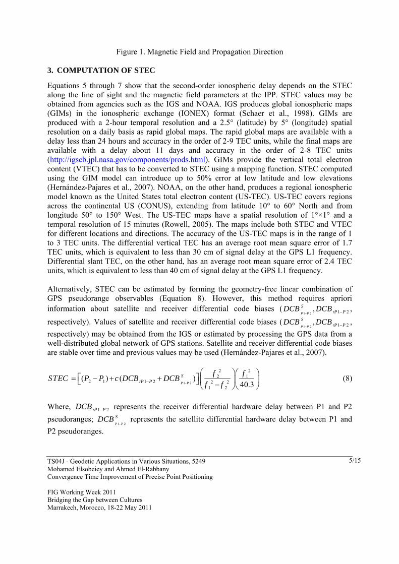
field at the ionospheric pierce point (IPP), i.e., the intersection of the line of sight with the ionospheric single layer at height hion; and is the angle between the magnetic field and the propagation direction (Figure 1).

X

Y

B0

θPiercePoint

Satellite

hion

Receiver

z

z'Z

Rα


5/15

Figure 1. Magnetic Field and Propagation Direction 3. COMPUTATION OF STEC

Equations 5 through 7 show that the second-order ionospheric delay depends on the STEC along the line of sight and the magnetic field parameters at the IPP. STEC values may be obtained from agencies such as the IGS and NOAA. IGS produces global ionospheric maps (GIMs) in the ionospheric exchange (IONEX) format (Schaer et al., 1998). GIMs are produced with a 2-hour temporal resolution and a 2.5° (latitude) by 5° (longitude) spatial resolution on a daily basis as rapid global maps. The rapid global maps are available with a delay less than 24 hours and accuracy in the order of 2-9 TEC units, while the final maps are available with a delay about 11 days and accuracy in the order of 2-8 TEC units (http://igscb.jpl.nasa.gov/components/prods.html). GIMs provide the vertical total electron content (VTEC) that has to be converted to STEC using a mapping function. STEC computed using the GIM model can introduce up to 50% error at low latitude and low elevations (Hernández-Pajares et al., 2007). NOAA, on the other hand, produces a regional ionospheric model known as the United States total electron content (US-TEC). US-TEC covers regions across the continental US (CONUS), extending from latitude 10° to 60° North and from longitude 50° to 150° West. The US-TEC maps have a spatial resolution of 1°×1° and a temporal resolution of 15 minutes (Rowell, 2005). The maps include both STEC and VTEC for different locations and directions. The accuracy of the US-TEC maps is in the range of 1 to 3 TEC units. The differential vertical TEC has an average root mean square error of 1.7 TEC units, which is equivalent to less than 30 cm of signal delay at the GPS L1 frequency. Differential slant TEC, on the other hand, has an average root mean square error of 2.4 TEC units, which is equivalent to less than 40 cm of signal delay at the GPS L1 frequency. Alternatively, STEC can be estimated by forming the geometry-free linear combination of GPS pseudorange observables (Equation 8). However, this method requires apriori information about satellite and receiver differential code biases (

1 2 1 2, P P

SrP PDCB DCB ,

respectively). Values of satellite and receiver differential code biases (1 2 1 2, P P

SrP PDCB DCB ,

respectively) may be obtained from the IGS or estimated by processing the GPS data from a well-distributed global network of GPS stations. Satellite and receiver differential code biases are stable over time and previous values may be used (Hernández-Pajares et al., 2007).

1 2

2 22 1

2 1 1 2 2 21 2

( ) ( )40.3

P P

SrP P

f fSTEC P P c DCB DCB

f f (8)

Where, 1 2rP PDCB represents the receiver differential hardware delay between P1 and P2

pseudoranges; 1 2P P

SDCB represents the satellite differential hardware delay between P1 and

P2 pseudoranges.


6/15

4. MAGNETIC FIELD MODEL

Geomagnetic field of the Earth can be approximated by a magnetic dipole placed at the Earth’s centre and tilted 11.5° with respect to the axis of rotation. The magnetic field inclination is downwards throughout most of the northern hemisphere and upwards throughout most of the southern hemisphere. A line that passes through the centre of the Earth along the dipole axis intersects the surface of the Earth at two points, referred to as the geomagnetic poles. Unfortunately, dipole model accounts for about 90% of the Earth’s magnetic field at the surface (Merrill and McElhinny, 1983). After the best fitting geocentric dipole is removed from the magnetic field at the Earth’s surface, the remaining part of the field, about 10%, is referred to as non-dipole field. Both dipole and non-dipole parts of the Earth’s magnetic field change with time (Merrill and McElhinny, 1983). The dipole approximation is more or less valid up to a few Earth radii; beyond this distance limit the Earth’s magnetic field significantly deviates from the dipole field because of the interaction with the magnetized solar wind (Houghton et al., 1998). A more realistic model for the Earth’s geomagnetic field, which is used in this paper, is the international geomagnetic reference field (IGRF). The IGRF model is a standard spherical harmonic representation of the Earth's main field. The model is updated every 5 years. The international association of geomagnetism and astronomy (IAGA) has released the 11th generation of the IGRF in December 2009. The coefficients of the IGRF11 model are based on data collected from different sources, including geomagnetic measurements from observatories, ships, aircrafts, and satellites (NOAA, 2010). The relative difference between the dipole and IGRF models ranges from -20% in the east of Asia up to +60% in the so-called south Atlantic anomaly (Hernández-Pajares et al., 2007). 5. EFFECT OF SECOND-ORDER IONOSPHERIC DELAY ON THE

DETERMINATION OF SATELLITE ORBIT AND CLOCK CORRECTIONS

To investigate the effect of second-order ionospheric delay on the GPS satellite orbit and clock corrections, Bernese GPS software was used. A global cluster of 284 IGS reference stations (Figure 2) was formed based on a priori information about the behaviour of each receiver’s clock and the total number of carrier-phase ambiguities in the corresponding observation file. GPS measurements collected at the 284 IGS stations have been downloaded from the IGS website for DOY125 of 2010 (May 05, 2010). The raw data was first corrected for the second-order ionospheric delay using Equations 5 through 7. Equation 8 was used to compute the STEC values and the IGS published DCBs are applied. The corrected data along with the broadcast ephemeris were used as input to the Bernese GPS software to estimate the satellite orbit and clock corrections.


7/15

Figure 2. Global Cluster of IGS Stations Used to Estimate GPS Satellite Orbit, Satellite Clock Corrections, and GIMs

In comparison with the IGS final orbit, our results show that the effect of second-order ionospheric delay on GPS satellite orbit ranges from 1.5 to 24.7 mm in radial, 2.7 to 18.6 mm in the along-track, and 3.2 to 15.9 mm in cross-track directions, respectively (Figure 3).

Figure 3. Effect of Second-Order Ionospheric Delay on GPS Satellite Orbit

GPS Satellite

G02

G03

G04

G05

G06

G07

G08

G09

G10

G11

G12

G13

G14

G15

G16

G17

G18

G19

G20

G21

G22

G23

G24

G26

G27

G28

G29

G30

G31

G32

Orb

it D

iffe

renc

e (m

)

0.000

0.005

0.010

0.015

0.020

0.025

0.030

Radial Along-trackCross-track


8/15

Because only the difference between receiver and satellite clock parameters ( ) src dt dt

appears in the GPS observation equations, it is only possible to solve for the clock parameters in the relative sense. All clock parameters but one can be estimated, i.e., either a receiver or a satellite clock correction has to be fixed or selected as a reference. The only requirement is that the reference clock must be available for each epoch where the clock values are estimated (Dach et al., 2007). A reference clock should be easily modelled by an offset and a drift. A polynomial is fitted to the combined values of the clock corrections. In this way the time scale presented by the reference clock is the same for the entire solution. When the reference clock is synchronized to the GPS broadcast time, all aligned clocks to the reference clock will refer to the same time scale. All deviations of the real behaviour of the reference clock are reflected in all other clocks of the solution; therefore, the reference clock must be carefully selected. To determine the reference clock, Bernese GPS software fits a polynomial of the first-order as a default (with the option to use up to the 10th order) to all clocks and the mean RMS is computed. The reference clock is selected as the clock which leads to the smallest mean fit RMS and is available for all epochs. Our study showed that the effect of second-order ionospheric delay on the estimated satellite clock solution differences were within 0.067 ns (2 cm). These values are comparable to the corresponding values of the IGS analysis centres and the final IGS clock corrections. Figure 4 shows the RMS (in picoseconds) of the estimated satellites clock corrections compared with the corresponding values of the IGS final satellites clock corrections.

Figure 4. RMS of GPS Satellites Clock Corrections

GPS Satellite

G02

G03

G04

G05

G06

G07

G08

G09

G10

G11

G12

G13

G14

G15

G16

G17

G18

G19

G20

G21

G22

G23

G24

G26

G27

G28

G29

G30

G31

G32

Clo

ck R

MS

(ps

)

0

10

20

30

40

50

IGS Clock RMSEstimated Clock RMS


9/15

6. EFFECT OF SECOND-ORDER IONOSPHERIC DELAY ON PPP SOLUTION

The GPSPace PPP processing software, which was developed by Natural Resources Canada (NRCan), was modified to accept the second-order ionospheric correction. GPS data from 12 IGS stations (Figure 5) were processed using the modified GPSPace. The stations were chosen randomly and were not included in the satellite orbit and clock corrections estimation. The data used were the ionosphere-free (with both first- and second-order corrections included) linear combination of pseudorange and carrier-phase measurements. The estimated precise satellite orbit and clock corrections, from the previous step, were used in the data processing. The results show that improvements are attained in all three components of the station coordinates. Figures 6 through 11 show the 3D solutions obtained with and without the second-order ionospheric corrections included, for stations TAH1 and DRAG, as examples. As can be seen, the amplitude variation of the estimated coordinates during the first 15 minutes is reduced when considering the second-order ionospheric delay. In addition, the convergence time for the estimated parameters is reduced by about 15%. The final PPP solution shows an improvement in the order of 3 mm in station coordinates. It should be pointed out that the solution improvement is much higher at low latitudes where the second-order ionospheric effect is much higher. Table 1 summarizes the RMS of the final solution of all stations.

Figure 5. IGS Stations Used in Verification of the Estimated GPS satellite Orbit and Clock Corrections


10/15

Table 1: RMS of the Final Solution of the Tested IGS Stations

Processing Mode

1st Order IONO

RMS (mm) 1st and 2nd Order IONO

RMS (mm) Station Lat. Lon. Ht. 3D Lat. Lon. Ht. 3D BAN2 2.1 2.5 3.1 4.5 1 1.2 1.8 2.4 BUCU 1.2 2 2.6 3.5 0.8 1.9 2 2.9 DAEJ 2 2.2 2.9 4.2 0.5 0.8 1.3 1.6 DRAG 2.2 2.4 3.3 4.6 1.1 0.9 1.2 1.9 FLIN 2 2.1 2.3 3.7 1.8 1.9 2 3.3 GUAT 2 2.8 3.5 4.9 0.6 1.9 2.1 2.9 HARB 1.5 1.5 1.8 2.8 1.2 1.4 1.5 2.4 JPLM 1.1 1.8 1.9 2.8 1 1.5 1.6 2.4 LPGS 1.7 2.1 2.8 3.9 1.1 1.8 2 2.9 MOBS 1.5 1.7 2.2 3.2 1.2 1.4 1.8 2.6 NANO 1.8 2.2 2.7 3.9 1.2 2 2.5 3.4 TAH1 1.2 2.1 2.4 3.4 0.9 1.8 2 2.8

Figure 6. Latitude Improvement by Accounting for Second-Order Ionospheric Delay at DRAG IGS Station, DOY125, 2010

Time (Minutes)0 10 20 30 40 50 60

Lat

itude

Err

or (

m)

-0.4

-0.2

0.0

0.2

0.4

0.6

0.8

1.0

1.2

1.4

1.6

First-Order IONO Only First+Second-order IONO


11/15

Figure 7. Longitude Improvement by Accounting for Second-Order Ionospheric Delay at DRAG IGS Station, DOY125, 2010

Figure 8. Ellipsoidal Height Improvement by Accounting for Second-Order Ionospheric Delay at DRAG IGS Station, DOY125, 2010

Time (Minutes)

0 10 20 30 40 50 60

Lon

gitu

de E

rror

(m

)

-3.0

-2.5

-2.0

-1.5

-1.0

-0.5

0.0

0.5


Time (Minutes)0 10 20 30 40 50 60

Hei

ght E

rror

(m

)

-12

-10

-8

-6

-4

-2

0

2



12/15

Figure 9. Latitude Improvement by Accounting for Second-Order Ionospheric Delay at THA1 IGS Station, DOY125, 2010

Figure 10. Longitude Improvement by Accounting for Second-Order Ionospheric Delay at THA1 IGS Station, DOY125, 2010

Time (Minutes)0 10 20 30 40 50 60

Lat

itude

Err

or (

m)

-3

-2

-1

0

1

2

3


Time (Minutes)0 10 20 30 40 50 60

Lon

gitu

de E

rror

(m

)

-5

-4

-3

-2

-1

0

1

2



13/15

Figure 11. Ellipsoidal Height Improvement by Accounting for Second-Order Ionospheric Delay at THA1 IGS Station, DOY125, 2010

7. CONCLUSIONS

It has been shown that rigorous modelling of GPS residual errors can improve the PPP convergence time and solution. STEC derived from the code measurements on L1 and L2, along with the IGRF geomagnetic field model (IGRF11), were used to estimate the correction for the second-order ionospheric delay. A global cluster consisting of 284 IGS stations is used to estimate the GPS satellite orbit, clock corrections, and GIMs after accounting for the second-order ionospheric delay using Bernese GPS software. It has been shown that neglecting the second-order ionospheric delay can produce an orbital error ranging from 1.5 to 24.7 mm in radial, 2.7 to 18.6 mm along-track, and 3.2 to 15.9 mm in cross-track directions, respectively. As well, neglecting the second-order ionospheric delay results in a satellite clock error of up to 0.067 ns (i.e. equivalent to a ranging error of 2 cm). Furthermore, accounting for the second-order ionospheric delay can improve the final PPP 3D positioning solution by about 3 mm and improve the convergence time of the estimated parameters by about 15%. 8. ACKNOWLEDGMENTS

This research was supported in part by the GEOIDE Network of Centres of Excellence (Canada) and by the Natural Sciences and Engineering Research Council (NSERC) of Canada. The authors would like to thank the Geodetic survey division of NRCan for providing the source code of the GPSPace PPP. The data sets used in this research were obtained from the IGS website http://igscb.jpl.nasa.gov/.

Time (Minutes)0 10 20 30 40 50 60

Hei

ght E

rror

(m

)

-2

-1

0

1

2

3

4



14/15

9. REFERENCES

Bassiri, S. and G. Hajj, 1993. High-order ionospheric effects on the global positioning system observables and means of modeling them, Manuscr. Geod., 18, pp 280– 289

Dach, R., U. Hugentobler, P. Fridez, and M. Meindl, 2007. Bernese GPS Software Version 5.0. Astronomical Institute, University of Berne, Switzerland.

Gutman, S., T. Fuller-Rowell, D. Robinson, 2003. Using NOAA Atmospheric Models to Improve Ionospheric and Tropospheric Corrections. U.S. Coast Guard DGPS Symposium, Portsmouth, VA, 19 June.

Hernández-Pajares, M., J. M. Juan, J. Sanz, and R. Orús, 2007. Second-order Ionospheric Term in GPS: Implementation and Impact on Geodetic Estimates. Journal of Geophysical Research, VOL. 112, B08417

Hofmann-Wellenhof, B., H. Lichtenegger, and E. Walse, 2008. GNSS Global Navigation Satellite Systems; GPS, Glonass, Galileo & more. Springer Wien, New York

Hoque, M. and N. Jakowski, 2007, Higher order ionospheric effects in precise GNSS positioning. Journal of Geodesy Vol. 81, pp 259-268.

Hoque, M. and N. Jakowski, 2008. Mitigation of higher order ionospheric effects on GNSS users in Europe. GPS solutions Vol. 12, No. 2, pp 87-97.

Houghton, J. T., M. J. Rycroft, and A. J. Dessler, 1998. Physics of the space environment. Cambridge University Press, 1998.

Leick, A., 2004. GPS Satellite Surveying. 3rd edition, John Wiley and Sons.

Lutz, S., S. Schaer, M. Meindl, R. Dach, and P. Steigenberger, 2010. Higher-order Ionosphere Modeling for CODE’s Next Reprocessing Activities. Proceeded in the IGS Analysis Centre Workshop, Newcastle upon Tyne, England , 28 June – 2 July 2010

Merrill, R. T. and M. W. McElhinny, 1983. The Earth’s Magnetic Field, its History, Origin and Planetary Perspective. International Geophysics series, Volume 32. Academic press Inc

National Oceanic and Atmospheric Administration (NOAA) website, http://www.ngdc.noaa.gov/IAGA/vmod/igrf.html. Accessed June 2010

Rowell, T. F., 2005. USTEC: a new product from the Space Environment Centre characterizing the ionospheric total electron content. GPS Solutions, Springer-Verlag. Vol. 9, pp. 236-239.

Schaer, S., G. Beutler, and M. Rothacher, 1998. Mapping And Predicting The Ionosphere. Proceeded in the IGS Analysis Centre Workshop, Darmstadt, Germany, February 9–11


15/15

Schaer, S., S. Steigenberger, 2006. Determination and Use of GPS Differential Code Bias Values. IGS Analysis Centre Workshop, Darmstadt, Germany.

BIOGRAPHICAL NOTES

Mohamed Elsobeiey is a Ph.D. candidate in the Department of Civil Engineering (Geomatics Engineering Program), Ryerson University. He has a B.Sc. and M.Sc. in Civil Engineering from Zagazig University, Egypt. He is interested in navigation and satellite positioning software development. Dr. Ahmed El-Rabbany obtained his PhD degree in GPS from the Department of Geodesy and Geomatics Engineering, University of New Brunswick. He is currently a professor and the graduate program director at Ryerson University in Toronto, Canada. He also holds an Honorary Research Associate position at the Department of Geodesy and Geomatics Engineering, University of New Brunswick. His areas of expertise include satellite positioning and navigation, integrated navigation systems, and hydrographic surveying. Dr. El-Rabbany authored an easy-to-read GPS book, which received a 5-star rating on the Amazon website and was listed as a bestselling GPS book. He also published numerous journal and conference papers. Dr. El-Rabbany received a number of awards in recognition of his academic achievements, including three merit awards from Ryerson University.

CONTACTS

Mohamed Elsobeiey

Dept. of Civil Engineering Ryerson University 350 Victoria Street, Toronto, Ontario, Canada M5B 2K3 Tel. +1 (416) 979-5000 ext. 6472 Fax +1 (416) 979-5122 Email: [email protected] Dr. Ahmed El-Rabbany Department of Civil Engineering Ryerson University 350 Victoria Street, Toronto, Ontario, Canada M5B 2K3 Tel. +1 (416) 979-5000 ext. 6472 Fax +1 (416) 979-5122 Email: [email protected] Web site: http://www.civil.ryerson.ca

convergence time improvement of precise point positioning · convergence time improvement of...

Documents