Department of Economics, Umeå University, S-901 87, Umeå, Sweden

www.cere.se

CERE Working Paper, 2014:15

Convergence in global environmental performance

Assessing country heterogeneity Runar Brännlund and Amin Karimu

Centre for Environmental and Resource Economics

Umeå School of Economics and Business

Umeå University

The Centre for Environmental and Resource Economics (CERE) is an inter-disciplinary and inter-university research centre at the Umeå Campus: Umeå University and the Swedish University of Agricultural Sciences. The main objectives with the Centre are to tie together research groups at the different departments and universities; provide seminars and workshops within the field of environmental & resource economics and management; and constitute a platform for a creative and strong research environment within the field.

i

Convergence in global environmental performance

Assessing country heterogeneity

Runar Brännlund and Amin Karimu

Centre for Environmental and Resource Economics Umeå School of Economics and Business

Umeå University

 

 

Abstract A large body of literature explores convergence in environmental performance (EP) using a simple measure of the percentage change of per capita CO2 as dependent variable and the level of per capita CO2 and GDP as explanatory variables. As such it conforms to the standard convergence literature in the economic growth literature. This study differs from these studies by constructing a measure based on production theory, where production processes explicitly results in the production of two outputs; a good output (GDP) and a bad output (CO2). Based on this we derive an EP index that can be expressed as the ratio of the inverse of the change of the emission intensity. We use the derived EP index to test the β-convergence hypothesis for a panel of 94 countries. The results reveal strong evidence in support of β-convergence in environmental, or carbon, performance. Moreover we find evidence of heterogeneity between groups of countries in line with the concept of “club” convergence and also heterogeneity between countries within country groups, especially for the high-income group. Additionally, we find evidence of a negative relation between environmental performance and fossil fuel share both at the global level as well as within sub-samples, which tend to vary with capital intensity. As such the results conform to the results from studies of the dynamics of per capita emissions. These results are therefore very informative and can help in both regional and international negotiations regarding burden sharing of global CO2 emissions. The results also suggest a balanced policy mix between efficiency and conservation policies in order to promote good environmental performance.

Keywords: Convergence, Environmental Performance, Fossil fuel, Kyoto Protocol,

Spillovers

JEL Classification:

1

1. Introduction

The impact of economic activity on the environment is attracting increasing attention from

policy makers, firms and the academia. This is partly due to the increasing evidence of the

negative impact that human activity have on the environment. Furthermore, there has been an

increasing interest concerning the dynamic properties of emissions; how they change over time

as a result of changes in income, income distribution, technical development, etc. As a result of

the latter a number of studies have been carried out to analyze the relationship between

economic growth and changes of emission based on the Environmental Kuznets Curve

hypothesis (EKC). The EKC hypothesis states that environmental degradation follows an

inverted U-shaped relationship as a country’s GDP grows over time (Grossman and Krueger,

1991, 1995). Comprehensive reviews of the EKC literature can be found in Levinson (2002),

Dinda (2004), Stern (2004), Lieb (2004) and Kijima et al. (2010).

A recent strand in the literature is related to finding an appropriate measure for environmental

performance (EP), as an assessment tool for economic and environmental policy, and to assess

if EP converges across countries and over time for a given country. Whether there is

convergence or not in EP across countries has implications for future global emissions

negotiations, such as the Kyoto protocol in terms of quota allocations and also on regional level

negotiations. Therefore having an appropriate measure of EP and consequently providing

evidence for convergence/divergence is extremely important. The majority of the studies in

this strand of the literature measure EP using CO2 emissions as a ratio of population, GDP or

energy consumption. Recent papers in this line of research includes; Strazicich and List (2003),

Ngugen (2005), Aldy (2006, 2007), Ezcerra (2007), Panopoulou and Pantelidis (2007)

Camarero et al. (2008), Westerlund and Basher (2008), Brock and Taylor (2010), Camarero et

al. (2012), and Brännlund et.al (2014a). These studies implemented various econometric

methods from both parametric to non-parametric approaches to address the question of

convergence in environmental performance measured simply as per capita CO2 emissions, as a

ratio of GDP or energy consumption. However, according to Ramanathan (2002) these studies

only provide a partial picture of environmental performance as they only consider emissions

originating from economic activities.

There are other existing approaches in measuring environmental performance, as an alternative

to these measures. These other approaches in measuring EP are diverse but can be grouped into

three main perspectives, (1) the product cycle analysis/assessment, (2) the environmental

2

accounting perspective, and (3) the production theory framework. Each of these approaches

focus on different aspects of EP, albeit with different strengths and weaknesses, which are well

documented in Tyteca (1996) and Olsthoorn et al. (2001).

Our focus in this paper is to propose to use a simple but relevant theory for measuring EP, that

is based on production theory, inspired by recent work that includes Färe et al. (2006), Zaim

and Taskin (2000), Zofio and Prieto (2001), Zaim (2004), Zhou et al.(2006) and Picazo-Tadeo

and García-Reche (2007). Therefore our paper makes three key contributions to the literature.

Firstly, we propose to use a simple theory in measuring EP that explicitly considers that the

production process simultaneously results in both good and bad outputs. This framework is

based on Färe et al. (2006). Secondly, based on this, we calculate, in a first step, an EP index

for each country for a sample of 94 countries for the period (1971 to 2008). In a second step we

use the EP index in a regression analysis in order to test for β-convergence in environmental

performance. As far as we know we are among the first to do this based on a production theory

framework. The only paper in the literature that studied convergence based on the production

theory framework is Camarero et al. (2008) and Brännlund et al. (2014), but unlike our paper,

Camarero et al. focus only on a sample of OECD countries, while Brännlund et al. focus on

Swedish industries. Hence our work can therefore be seen as an extension of Camarero et al.

(2008) on two fronts; it extends to a global sample, and it looks specifically at it from a β-

convergence perspective as done in Brännlund et al. (2014) for Swedish industries.

Thirdly, we also consider heterogeneity in the rate of convergence both between groups of

countries, in line with “club” convergence, and also between countries. This is important for

both regional and international negotiations regarding burden sharing in global environmental

emissions, especially CO2 emissions. It is important to know the contributions to growth in CO2

emissions by regions and by countries to aid the negotiations in burden sharing of global CO2

emissions. We also use econometric techniques that accommodate both country and time

specific effects that help to reduce spillover effects (cross-sectional dependence) from common

shocks, and therefore reduce the possible bias that spillover effects can generate on the

estimated parameters and also reduces possible cofounding effects.

The rest of the paper is organized as follows. Section two provides the theory and method for

measuring the EP index, and section three provides details on the empirical approach for the

study. The data is presented in section four, and the results are presented in section five.

3

Section six, finally, contains some concluding comments and policy implications from the

study.

2. Theory and method

The theoretical approach outlined here follows primarily Färe et al. (2006). The theory as such

is thus not novel, and the theoretical presentation here is motivated mainly to lay the foundation

to the performance index that will be used subsequently in the empirical analysis.1

In particular the environmental performance index, EP, that will be used here is based on

neoclassical production theory, which explicitly recognize that the production process results in

both good and bad outputs. More specifically, this means that we will use a quantity approach

based on ratios of output distance functions. In this particular case, with one good (GDP) and

one bad (CO2) output it turns out that this ratio of distance functions results in a simple

expression showing the growth path of the inverse of the emission intensity.

The distance functions are here defined on the output possibility set, P(x), expressed as

. Here y is good output, b is bad output, and x a vector of

inputs. In general y and b are vectors. P(x) is assumed to be convex, closed, and bounded, i.e.,

compact, with inputs and good outputs being freely disposable. Good outputs being freely

disposable is formally expressed as , which means

that a good output can always be reduced without reducing any other output.

In addition to these technological properties, shaping the frontier of P(x), additional properties

must be introduced to distinguish good outputs from bad outputs. Firstly, good and bad outputs

are assumed to be weakly disposable. This means that good and bad outputs can always be

simultaneously reduced proportionally. Since bad outputs are weakly disposable, a reduction in

a bad output, or emissions, cannot be accomplished without giving up some good output

directly or indirectly (Färe et al., 2006, p. 261).

A second technological property, imposed to distinguish good outputs from bad outputs, is that

(y, b) is null-joint, i.e. good output cannot be produced without producing any bad output.In

order to form a good output quantity index, Shephard output distance functions are defined for

1 See also Brännlund & Lundgren (2014), and Brännlund et.al. (2014), for applications on Swedish industry data.

{ }),( producecan :),()( byxbyxP =

)(),( then and )(),( xPbyyyxPby ∈′≤′∈

4

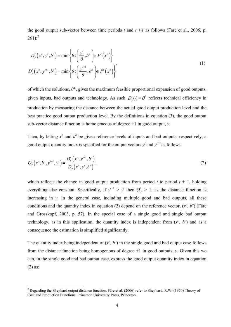
the good output sub-vector between time periods t and t +1 as follows (Färe et al., 2006, p.

261):2

( ) ( )

( ) ( )1

1

, , min : ,

, , min : ,

tt o t o o t oy

tt o t o o t oy

yD x y b b P x

yD x y b b P x

θθ

θθ

++

⎧ ⎫⎛ ⎞⎪ ⎪= ∈⎨ ⎬⎜ ⎟⎪ ⎪⎝ ⎠⎩ ⎭⎧ ⎫⎛ ⎞⎪ ⎪= ∈⎨ ⎬⎜ ⎟⎪ ⎪⎝ ⎠⎩ ⎭

, (1)

of which the solutions, θ*, gives the maximum feasible proportional expansion of good outputs,

given inputs, bad outputs and technology. As such *( )tyD θ⋅ = reflects technical efficiency in

production by measuring the distance between the actual good output production level and the

best practice good output production level. By the definitions in equation (3), the good output

sub-vector distance function is homogeneous of degree +1 in good output, y.

Then, by letting xo and bo be given reference levels of inputs and bad outputs, respectively, a

good output quantity index is specified for the output vectors yt and yt+1 as follows:

( ) ( )( )

11

, ,, , ,

, ,

t o t oyt o o t t

y t o t oy

D x y bQ x b y y

D x y b

++ = , (2)

which reflects the change in good output production from period t to period t + 1, holding

everything else constant. Specifically, if yt+1 > yt then Qty > 1, as the distance function is

increasing in y. In the general case, including multiple good and bad outputs, all these

conditions and the quantity index in equation (2) depend on the reference vector, (xo, bo) (Färe

and Grosskopf, 2003, p. 57). In the special case of a single good and single bad output

technology, as in this application, the quantity index is independent from (xo, bo) and as a

consequence the estimation is simplified significantly.

The quantity index being independent of (xo, bo) in the single good and bad output case follows

from the distance function being homogenous of degree +1 in good outputs, y. Given this we

can, in the single good and bad output case, express the good output quantity index in equation

(2) as:

2 Regarding the Shephard output distance function, Färe et al. (2006) refer to Shephard, R.W. (1970) Theory of Cost and Production Functions. Princeton University Press, Princeton.

5

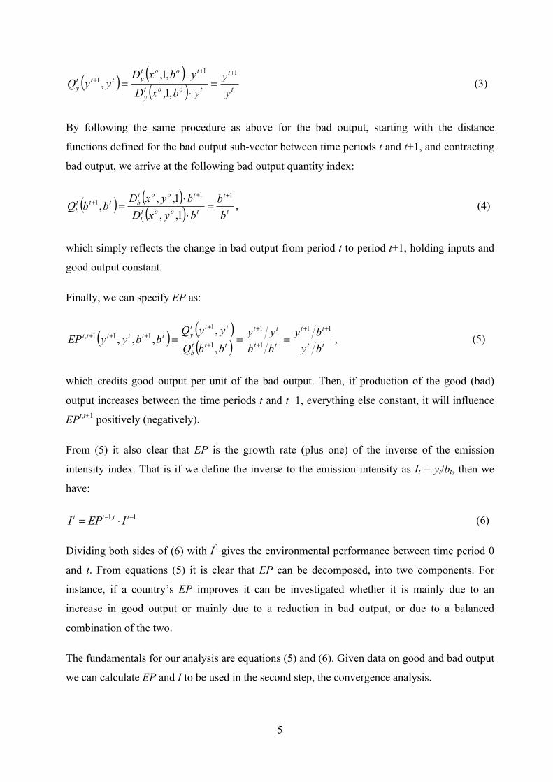
( ) ( )( ) t

t

tooty

tootyttt

y yy

ybxDybxD

yyQ11

1

,1,,1,

,++

+ =⋅⋅

= (3)

By following the same procedure as above for the bad output, starting with the distance

functions defined for the bad output sub-vector between time periods t and t+1, and contracting

bad output, we arrive at the following bad output quantity index:

( ) ( )( ) t

t

tootb

tootbttt

b bb

byxDbyxD

bbQ11

1

1,,1,,

,++

+ =⋅⋅

= , (4)

which simply reflects the change in bad output from period t to period t+1, holding inputs and

good output constant.

Finally, we can specify EP as:

( ) ( )( ) tt

tt

tt

tt

tttb

tttytttttt

byby

bbyy

bbQyyQ

bbyyEP11

1

1

1

1111,

,,

,,,++

+

+

+

++++ === , (5)

which credits good output per unit of the bad output. Then, if production of the good (bad)

output increases between the time periods t and t+1, everything else constant, it will influence

EPt,t+1 positively (negatively).

From (5) it also clear that EP is the growth rate (plus one) of the inverse of the emission

intensity index. That is if we define the inverse to the emission intensity as It = yt/bt, then we

have:

1, 1t t t tI EP I− −= ⋅ (6)

Dividing both sides of (6) with I0 gives the environmental performance between time period 0

and t. From equations (5) it is clear that EP can be decomposed, into two components. For

instance, if a country’s EP improves it can be investigated whether it is mainly due to an

increase in good output or mainly due to a reduction in bad output, or due to a balanced

combination of the two.

The fundamentals for our analysis are equations (5) and (6). Given data on good and bad output

we can calculate EP and I to be used in the second step, the convergence analysis.

6

3. Empirical approach

The empirical analysis is performed in two steps. First we specify and calculate the EP index at

country level. In the second step we specify a typical “growth equation” with EP as the

dependent variable and I as the independent variable together with other control variables, such

as capital and fossil fuels use. The choice of controls is based on production theory where each

production process depends on a given technology that combines effective capital, energy and

labor services to produce a unit of output and in the process of converting the inputs (effective

capital and energy) also generate pollution. This production process at the firm level can be

aggregated to the macro-level to provide aggregate output and emissions levels that are

generated from input combination via a given level of technology. We therefore assume

environmental performance to depend on the inverse of the initial emission intensity, capital

and fossil fuel use, where fossil fuels is used as a proxy for energy use, since most of the

emissions is generated from the use of fossil fuels.

The main focus of this study is to examine the convergence hypothesis, specifically,

convergence in EP (growth in the inverse of CO2 intensity) by analyzing a cross-country data

than spans a period of over 30 years. Three main approaches are commonly applied to analyses

the convergence hypothesis both in the environmental and economic growth literature. In this

study, however, we focus on the β-convergence approach in a panel data framework. Formally

we specify the basic empirical model as:

, , 1 1 , 2 , ,ln ln ln ln ,

1,... , 1,....

i t i t i t i t i t i tEP I K FF

i N Countries t T time periods

α φ β γ γ ε−= + + + + +

= = = = (7)

where β is the convergence parameter (the parameter of our central interest), 1tI − is the initial

level of the inverse in emission intensity, lnKi,t is capital in logs and lnFFi,t is fossil fuel use in

logs.3 Our interest is to test the hypothesis that β < 0, which, if the hypothesis holds, implies the

existence of so-called β-convergence. This means that countries with relatively low level of the

inverse of initial emissions intensity (high level of emission intensity) tends to grow faster in

terms of environmental performance, and hence tend to catch up with countries that start at a

3 Note that this is a year-to-year, panel data specification of convergence. Alternatively we could specify a cross-sectional model that relates the mean of the environmental performance index over a time period to an initial time period intensity level.

7

higher initial level of inverse of emissions intensity. If this is the case it may be because the low

performance countries can benefit from the experience and technologies developed and used by

the high performers. We also include time specific effects (ϕt) as well as country specific

effects (αi) to account for unobservables that are time specific and country specific,

respectively. Thus, if β < 0, αi = α for all i, and γ1 = γ2 = 0, then we have what has been called

absolute convergence, i.e. all countries converges to the same inverse emission intensity level.

If the above does not hold true, apart from β < 0, we have what has been called conditional

convergence, which means that the growth paths differs, and hence do not converge to the same

emission intensity level.

Further, to allow for more flexibility and to account for heterogeneity in convergence, a more

general specification of equation (7) is proposed that can be expressed as;

ln EPi,t = α i +φt +β ln Ii,t−1 + γ 1 ln Ki,t + γ 2 ln FFi,t + γ 3 ln Ii,t−1 ⋅ ln Ki,t + γ 4 ln Ii,t−1 ⋅ ln FFi,t +

γ 5 ln Ki,t ⋅ ln FFi,t + ε it

(8)

The convergence parameter, corresponding to β in equation (7), is then found by taking the

partial derivative of equation (8) with respect to the inverse of the initial emission intensity.

Correspondingly the effect on EP from the level of fossil fuel use is the derivative with respect

to fossil fuel use:

3 4 ,, 1

2 4 , 1 5

ln ln ln

ln ln ln .ln

itit i t

i t

iti t it

it

EP K FFIEP I KFF

β γ γ

γ γ γ

−

−

∂ = + +∂∂ = + +∂

%

%

As a result, using equation (8) allows the rate of convergence to vary between countries due to

differences in capital intensity and fossil fuel use.

The specifications, as presented in equation (7) and (8), are estimated using a fixed effects

model (time and country) due to the following reason. Firstly, we do not think that country

specific unobservables, such as norms or culture, are uncorrelated with the explanatory

variables such as the inverse of emissions intensity or capital. It is most likely that norms and

culture influence how policies are adopted to influence capital accumulation and its association

with labor and the combination of this on output-emissions relations. Secondly, given the long

time period, times series proprties cannot be ignored. We assess this via various diagnostic tests

8

on the residual to check for stationarity and also check for cross-sectional dependence. We also

include time fixed effects that can capture common factors that are time specific since it

otherwise could lead to spillover effects (cross-sectional dependence), which may lead to

biased estimates in either direction. It is important to clarify that the time fixed effects cannot

account for all forms of common factor effects, but only for time specific common factors.

4. Data

The data used for the analysis is a panel data set covering 1971 to 2008 for 94 countries (list of

the countries is presented in Table A1 in the appendix) and includes data on CO2 emissions in

kilo tons, gross domestic product (GDP) in constant 2000 US dollars, gross fixed capital as a

ratio of GDP, total fossil fuels as a ratio of total energy use. All variables are taken from the

World Development Indicator (WDI) database of the World Bank. The CO2 data together with

the GDP are used to calculate, or construct, the environmental performance index.

The CO2 data were originally gathered and developed by Marland et al. (1989), and were

constructed as estimates of CO2 emissions from fossil burning and manufacturing of cement.

This method was adopted by the World Bank in the construction of the recent CO2 series. One

shortcoming of this data series is that it omits carbon dioxide emissions stemming from

deforestation, land-use changes, and the burning of wood fuel. But irrespective of this, we think

this variable is reliable, and most of all consistent across the world and can reasonable

approximate global CO2 emissions despite an error of uncertainty of 6-10% (Strazicich and

List, 2003).

The data on capital is constructed based on capital investments that include plant, machinery

and equipment purchases, land development, rail and road constructions, buildings, and net

acquisition of valuables. The capital variable is expressed as a ratio of GDP. It is possible that

some of the variables included in the construction of the capital stock might not directly require

energy services in their use but might do so in their production and therefore their contribution

to CO2 emissions might be due to both processes (consumption and production).

9

Fossil fuel data comprises of coal, oil, petroleum, and natural gas products, expressed as a ratio

of total energy use. Total energy use data is constructed from primary energy use that includes

indigenous production plus imports and stock changes, and excludes exports and fuels supplied

to ships and aircraft engaged in international transport. It is expressed in kilo tons of oil

equivalents.

Summary statistics for the variables used for the analysis, which is presented in Table 1, reveals

a large variation between countries for all variables. The variability of each of the variables is

shown by the standard deviation with large values indicating more variability. Furthermore, we

calculated the cumulative EP (geometric mean) and its two components (good output and bad

output) and presented in figure 1. The figure indicates that before 1990, changes in bad output

(cumulative) tend to dominate changes in good output and consequently result in lower

environmental performance in relative terms. However, after 1990, the changes in bad output is

lower relative to changes in good output and implies higher environmental performance, which

appear to indicate decoupling between GDP (good output) and CO2 (bad output) after the

1990s.The implication of this is that over the years, both production and consumption

technologies have either become more efficient in the use of fossil energy, or that a shift has

occurred towards more use of non-fossil energy, or both.  

Table 1. Summary statistics for 94 countries, 1971-2008. Variable Obs Mean Std. Dev. Min Max CO2 (in 1000) 3570 189.3656 631.0257 .022002 7035.444 GDP (in 1000) 3572 273074.9 810098.5 448.0554 9532562 Fossil energy (in 1000) 3562 59.94908 203.7318 0.060494 2000.829 Capital (% GDP) 3494 21.70239 6.285652 2.000441 60.56181 EPI 3476 1.0108934 .1476797 .2634722 4.322163

The world GDP series also depicts a positive trend over the period under study, implying that at

the global level the world is producing more goods and services over time, which then put more

pressure on the use of energy, especially fossil energy with consequences on CO2 emissions.

However, the gap between the mean GDP series and that of CO2 widens over time. This

relationship provides some evidence of a decoupling between CO2 and GDP. The upper panel

in figure 1 also reveals a positive relationship between GDP and the CO2 series but with

different slopes, implying that other factors in addition to GDP influences the trend dynamics

of global CO2 emissions.

4 Is the geometric mean

10

Figure 1: Cummulative EP and its components (good output and bad output)

5. Results

Given the construction, or calculation, of the EP and the inverse of the emission intensity index

according to equations (5) and (6), the empirical strategy in our analysis follow a two-step

procedure: firstly, we will estimate equation (7) using the whole panel to examine the β-

convergence hypothesis, while allowing for heterogeneity in the convergence parameter via

interaction terms between previous I, K, and FF (inverse in emission intensity, capital and

share of fossil fuel use); secondly, we divide the sample into three groups of countries (low

income, middle income and high income) based on per capita income levels consistent with the

World Bank classification. The idea is to assess if the test for β-convergence is sample

dependent, and to examine possible heterogeneity in β-convergence in line with the so call

“club” convergence by testing if countries with different per capita income levels converge

differently or otherwise.

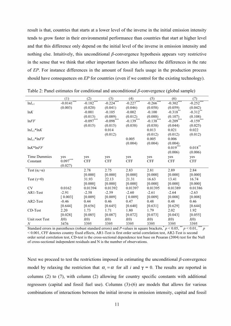
The results presented in Table 2 is based on the global sample, where we first test for

unconditional β-convergence by estimating equation (7) and (8) with the restriction that

for all i and γ = 0. The results for the unconditional β-convergence are presented in column (1)

in Table 2. The estimated coefficient of the inverse in the initial emission intensity (the β-

convergence) parameter is negative and significant at the 5% level. The implication of this

.7.8

.91

1.1

1970 1980 1990 2000 2010Year

Cummulative EPI Cummulative Good OutputCummulative Bad Output

α i =α

11

result is that, countries that starts at a lower level of the inverse in the initial emission intensity

tends to grow faster in their environmental performance than countries that start at higher level

and that this difference only depend on the initial level of the inverse in emission intensity and

nothing else. Intuitively, this unconditional β-convergence hypothesis appears very restrictive

in the sense that we think that other important factors also influence the differences in the rate

of EP. For instance differences in the amount of fossil fuels usage in the production process

should have consequences on EP for countries (even if we control for the existing technology).

Table 2: Panel estimates for conditional and unconditional β-convergence (global sample) (1) (2) (3) (4) (5) (6) (7) lnIt-1 -0.0141*** -0.182*** -0.224*** -0.227*** -0.266*** -0.302*** -0.252*** (0.003) (0.020) (0.041) (0.046) (0.058) (0.059) (0.042) lnK -0.001 -0.105 -0.002 -0.100 -0.318** -0.312** (0.013) (0.089) (0.012) (0.088) (0.107) (0.108) lnFF -0.097*** -0.098*** -0.139*** -0.138*** -0.209*** -0.159*** (0.015) (0.015) (0.038) (0.038) (0.044) (0.025) lnIt-1*lnK 0.014 0.013 0.021 0.022 (0.012) (0.012) (0.012) (0.012) lnIt-1*lnFF 0.005 0.005 0.006 (0.004) (0.004) (0.004) lnK*lnFF 0.019*** 0.018** (0.006) (0.006) Time Dummies yes yes yes yes yes yes yes Constant 0.097*** CFF CFF CFF CFF CFF CFF (0.027) Test (αi=α) 2.78 2.75 2.83 2.81 2.89 2.84 [0.000] [0.000] [0.000] [0.000] [0.000] [0.000] Test (γ=0) 31.93 22.13 21.31 16.63 13.41 16.74 [0.000] [0.000] [0.000] [0.000] [0.000] [0.000] CV 0.0162 0.01394 0.01392 0.01397 0.01395 0.01389 0.01386 AR1-Test -2.91 -2.58 -2.59 -2.60 -2.61 -2.64 -2.63 [ 0.003] [0.009] [0.009] [ 0.009] [0.009] [0.008] [0.008] AR2-Test -0.46 0.44 0.46 0.47 0.48 0.48 0.46 [0.644] [0.656] [0.645] [0.640] [0.631] [0.629] [0.644] CD-Test 2.20 1.73 1.71 1.80 1.79 2.02 1.92 [0.028] [0.085] [0.087] [0.072] [0.073] [0.043] [0.055] Unit root Test I(0) I(0) I(0) I(0) I(0) I(0) I(0) N 3476 3395 3395 3395 3395 3395 3395 Standard errors in parentheses (robust standard errors) and P-values in square brackets,* p < 0.05, ** p < 0.01, *** p < 0.001, CFF denotes country fixed effects, AR1-Test is first order serial correlation test, AR2-Test is second order serial correlation test, CD-test is the cross-sectional dependence test base on Pesaran (2004) test for the Null of cross-sectional independent residuals and N is the number of observations.

Next we proceed to test the restrictions imposed in estimating the unconditional β-convergence

model by relaxing the restriction that for all i and γ = 0. The results are reported in

columns (2) to (7), with column (2) allowing for country specific constants with additional

regressors (capital and fossil fuel use). Columns (3)-(6) are models that allows for various

combinations of interactions between the initial inverse in emission intensity, capital and fossil

α i =α

12

fuel, while column (7) reports the results for a model that adds interaction between fossil fuel

use and capital to the model in column (3). The test that is rejected for each of the

models presented in column (2) to (7), also the test that γ = 0 is rejected at the 5% level of

significance, implying that the unconditional β-convergence is not appropriate in exploring the

β-convergence hypothesis for this study. Henceforth we will therefore focus on the conditional

β-convergence hypothesis. However in order to discriminate between the conditional β-

convergence models, we apply cross-validation (CV) criteria to the models presented in

columns (2) to (7) and base our conclusions on the model with the smallest CV value as well as

correcting for cross-section dependence. The CV values show little differences but indicate

that the model presented in column 7 has the smallest CV value and also the errors do not

suffer from cross-sectional dependence at the 5% significance level, hence we focus our

interpretation on the results presented in column 7 in Table 2.

The results from the preferred model indicate evidence of conditional β-convergence in

environmental convergence, as the coefficient of the inverse of the initial emission intensity is

significantly negative. Further, the results indicates that the convergence parameter does not

vary with the level of capital for the global sample, since the coefficient of the interaction term

between the inverse of the initial emission intensity and that of capital is insignificant. The

capital elasticity is -0.3, which is significant at the 5% level and implies that capital, on

average, tend to reduce environmental performance. The implication of this is that the carbon

energy conservation investments that have been undertaken are not large enough to offset the

additional amount of carbon that is needed for having more capital, and as a consequence the

energy requirements outweigh the energy saving potentials from these investments.

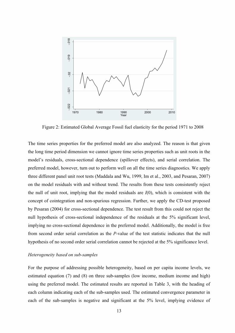
The estimated effect on EP from the fossil fuel share, on the other hand, depends on the capital

stock since the interaction effect is statistically significant. The fossil fuel share elasticity is

then calculated by taking the partial derivative of EP with respect to the fossil fuel share, which

then varies over time and across country due to variation in the capital stock over time and

between countries. Figure 2 present the graph for the average global fossil fuel share elasticity,

and it shows variation from -0.21 to -0.02 for the period under study. The implication of this is

that, EP appears to be less responsive to changes in the global average fossil fuel share in 2008

relative to say 1971. One possible interpretation of this is that even if the share of fossil fuels

increases on average, its effect on EP has become smaller due to improvements in energy

efficiency/productivity. That is, more good output (y) for the same amount of bad outbut (b).

α i =α

13

Figure 2: Estimated Global Average Fossil fuel elasticity for the period 1971 to 2008

The time series properties for the preferred model are also analyzed. The reason is that given

the long time period dimension we cannot ignore time series properties such as unit roots in the

model’s residuals, cross-sectional dependence (spillover effects), and serial correlation. The

preferred model, however, turn out to perform well on all the time series diagnostics. We apply

three different panel unit root tests (Maddala and Wu, 1999, Im et al., 2003, and Pesaran, 2007)

on the model residuals with and without trend. The results from these tests consistently reject

the null of unit root, implying that the model residuals are I(0), which is consistent with the

concept of cointegration and non-spurious regression. Further, we apply the CD-test proposed

by Pesaran (2004) for cross-sectional dependence. The test result from this could not reject the

null hypothesis of cross-sectional independence of the residuals at the 5% significant level,

implying no cross-sectional dependence in the preferred model. Additionally, the model is free

from second order serial correlation as the P-value of the test statistic indicates that the null

hypothesis of no second order serial correlation cannot be rejected at the 5% significance level.

Heterogeneity based on sub-samples

For the purpose of addressing possible heterogeneity, based on per capita income levels, we

estimated equation (7) and (8) on three sub-samples (low income, medium income and high)

using the preferred model. The estimated results are reported in Table 3, with the heading of

each column indicating each of the sub-samples used. The estimated convergence parameter in

each of the sub-samples is negative and significant at the 5% level, implying evidence of

-.022

-.021

-.02

-.019

-.018

Foss

il Fu

el E

last

icity

( G

loba

l Ave

rage

)

1970 1980 1990 2000 2010Year

14

conditional convergence. However a chi-square test to check if the differences in the estimated

convergence parameter are significant reveals that both the low and middle income samples are

significantly different from the high income sample, but the difference between the low and

middle income sample is not significant.

Table 3: Panel estimates for conditional β-convergence (sub-samples based on income level) (2) (3) (4) Low Income Middle Income High Income lnIt-1 -0.397*** -0.351*** -0.873*** (0.064) (0.074) (0.238) lnK 0.190 -0.502* -2.318*** (0.266) (0.221) (0.700) lnFF -0.238* -0.201*** -0.252*** (0.106) (0.035) (0.061) lnIt-1*lnK -0.014 0.039 0.244** (0.018) (0.021) (0.080) lnK*lnFF -0.014 0.026** 0.043** (0.035) (0.009) (0.015) Time Dummies yes yes yes Country effects yes yes yes N 361 2349 682

Equality test for β in the three samples

Chsq-test ( low middle highβ β β= = ) 11.47 [0.000]

Chsq-test ( )low middleβ β= 0.24 [0.623]

Chsq-test ( low highβ β= ) 4.16 [0.041]

Chsq-test ( middle highβ β= ) 4.83 [0.027]

Standard errors in parentheses,* p < 0.05, ** p < 0.01, *** p < 0.001, we also tested the equality of β (the coefficient for lnIt-1) across the three sub-samples by combining the three estimates that allows for testing restrictions across different samples using chi-square test (the suest command in STATA allows for the combination of estimates across different samples), where Chsq is chi-square and the P-values in square brackets. Moreover, we find that the interaction term between capital and the inverse of initial emission

intensity to be significant only for the high income sample. The results are thus revealing

heterogeneity at the country level within the high income group (since the partial derivative of

EP with respect to the inverse of initial emission intensity depends on the level of capital). The

estimated rate of convergence for low income and middle income groups are -0.40 and -0.35,

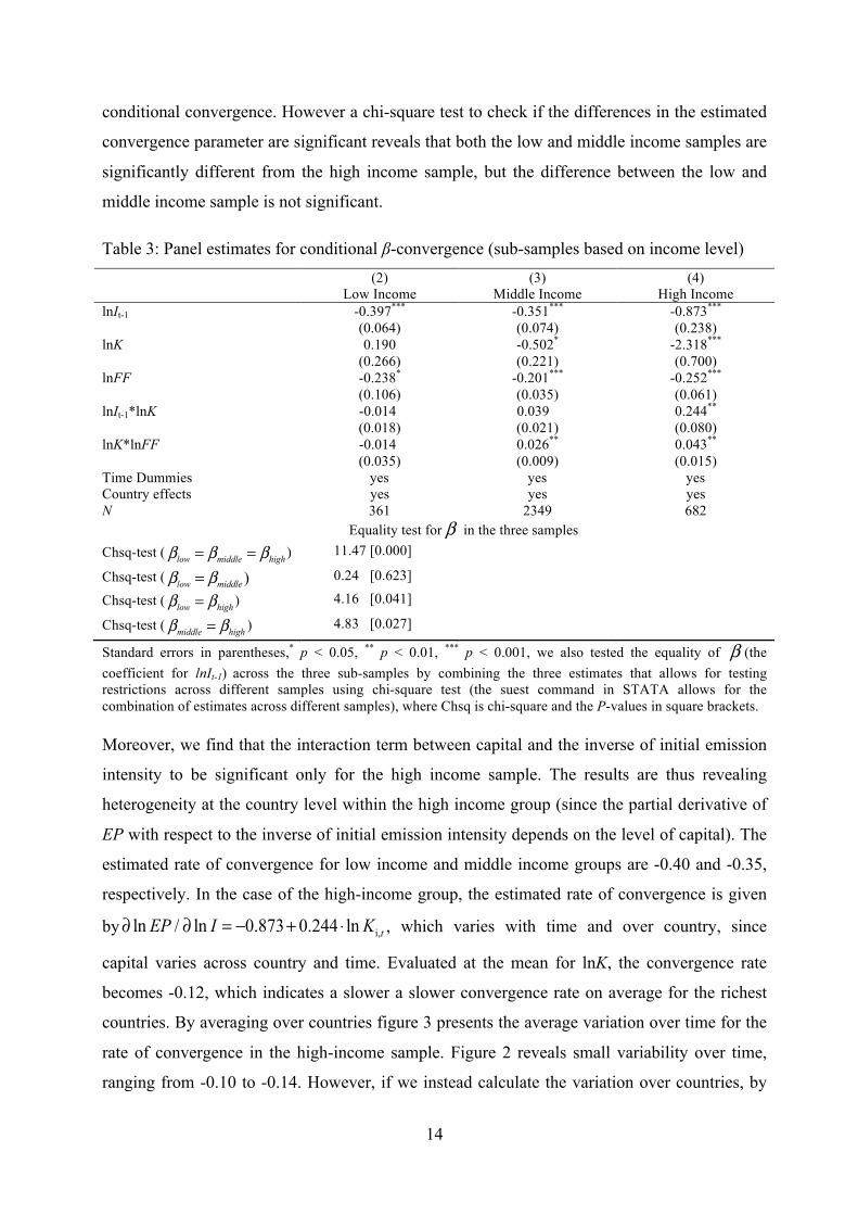
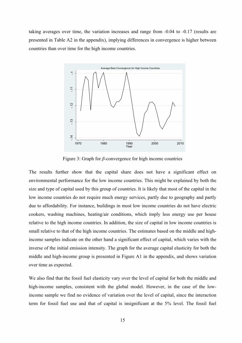
respectively. In the case of the high-income group, the estimated rate of convergence is given

by i,ln / ln 0.873 0.244 ln tEP I K∂ ∂ = − + ⋅ , which varies with time and over country, since

capital varies across country and time. Evaluated at the mean for lnK, the convergence rate

becomes -0.12, which indicates a slower a slower convergence rate on average for the richest

countries. By averaging over countries figure 3 presents the average variation over time for the

rate of convergence in the high-income sample. Figure 2 reveals small variability over time,

ranging from -0.10 to -0.14. However, if we instead calculate the variation over countries, by

15

taking averages over time, the variation increases and range from -0.04 to -0.17 (results are

presented in Table A2 in the appendix), implying differences in convergence is higher between

countries than over time for the high income countries.

Figure 3: Graph for β-convergence for high income countries

The results further show that the capital share does not have a significant effect on

environmental performance for the low income countries. This might be explained by both the

size and type of capital used by this group of countries. It is likely that most of the capital in the

low income countries do not require much energy services, partly due to geography and partly

due to affordability. For instance, buildings in most low income countries do not have electric

cookers, washing machines, heating/air conditions, which imply less energy use per house

relative to the high income countries. In addition, the size of capital in low income countries is

small relative to that of the high income countries. The estimates based on the middle and high-

income samples indicate on the other hand a significant effect of capital, which varies with the

inverse of the initial emission intensity. The graph for the average capital elasticity for both the

middle and high-income group is presented in Figure A1 in the appendix, and shows variation

over time as expected.

We also find that the fossil fuel elasticity vary over the level of capital for both the middle and

high-income samples, consistent with the global model. However, in the case of the low-

income sample we find no evidence of variation over the level of capital, since the interaction

term for fossil fuel use and that of capital is insignificant at the 5% level. The fossil fuel

-.14

-.13

-.12

-.11

-.1

Rat

e of

Con

verg

ence

1970 1980 1990 2000 2010Year

Average Beta Convergence for High Income Countries

16

elasticity for the low-income sample is -0.24, which implies fossil fuel usage tend to have a

negative impact on environmental performance. We also calculated the average middle and

high income fossil fuel elasticity and these are presented in Figure 4. As can be seen, the

elasticity is lower on average, and varies slightly over time. One possible explanation to the

difference in fossil fuel share elasticity between low and high income countries is that high

income countries have a more carbon efficient technology, i.e. more good output can be

produced for the same amount of bad output.

Figure 4: Estimated average fossil fuel elasticity for middle and high income samples

Additionally, we also examine the effect of the Kyoto protocol on EP by including a dummy

for the Kyoto implementation period in equation (8). The results are reported in Table A3 in the

appendix and indicate evidence of a significant positive effect of Kyoto on EP for both the

global sample and each of the sub-samples. However, the results based on the sub-sample

reveal that the shifts are higher for the low and middle income countries in comparison to the

high income countries, irrespective of no specific binding commitments for the low income

countries. As a robustness check on the construction of the Kyoto dummy, we also used a

different dummy that consider both the implementation and signing period for the protocol (the

signing of the Kyoto protocol was in 1997, while its implementation takes effects in 2005). We

did not, however, find any significant differences in the results, hence we decided to only report

the results based only on the implementation period.

-.125

-.12

-.115

1970 1980 1990 2000 2010Year

Elasticity (high income countries) Elasticity(middle income countries)

Average Fossil Fuel Elasticity for High and Middle Income Countries

Foss

il Fu

el E

last

icity

17

From the results above we can draw a number of overall conclusions. Firstly, there is strong

evidence of conditional convergence in environmental performance (EP) on the global scale.

Secondly, in general, there is evidence of heterogeneity in convergence in EP both between

groups of countries, based on income level, and between countries within the high income

group. Thirdly, both the share of capital and the share of fossil fuel use tend to have a negative

effect on environmental performance, particularly for the middle and high income countries. To

achieve better EP more effort seems to be needed in both reducing the share of fossil fuels and

to increase the use of more energy efficient capital in both production and consumption

processes in the economy.

A potential important corollary from the results above is that the abatement costs, due to a

relative fast transition to a lower global emission path, may become very high and also vary

substantially between countries depending on the capital intensity and the current dependency

on fossil fuels. The reason for this is that if there is a hurry to stabilize the CO2 concentration

level, and hence urgent to quickly reduce emissions, then capital has to be replaced at a faster

rate than business as usual. As a result, overall abatement costs will increase, and in the

presence of large variations in convergence patterns multi-lateral agreements may be more

difficult to achieve. These kinds of difficulties may increase as more countries, especially in

Asia, is on a path of fast growth, implying among other things, an increase in capital intensity.

6. Conclusion  Three key issues are addressed in this study. Firstly, we provide a simple framework in the

construction of environmental performance (EP) based on production theory. The theory

provides an easy procedure in constructing an index that does not require much data in terms of

the relevant variables to construct the index. Secondly, we address the question of convergence

in EP at the global level, and thirdly address the question of possible heterogeneity in EP both

between groups of countries (in line with the so call “club convergence”) and between

countries.

Our findings can be summarized as follows. First, the simple theory shows that the EP index

we construct is simply the rate of change in the ratio of the inverse in emission intensity

(emission intensity is define as the ratio of CO2 emission over GDP). This is because the

production process is assumed to result in two outputs, a good output (GDP in this case) and a

bad output (CO2). Since our interest is in EP in relation to CO2 emissions, the construction of

the index via this approach is appropriate, given that the GDP variable capture most of the good

18

output in the economy and that the CO2 variable capture most of the CO2 emissions in

producing the good output. The emphasis here is on CO2 related EP, not EP in general.

Secondly, based on the constructed EP index, we tested both the unconditional and conditional

β-convergence hypothesis at the global level. Here we find strong evidence in support of

conditional β-convergence in EP in the global sample. This finding is consistent with the

finding in Brännlund et al. (2014), which finds evidence of convergence in EP for Swedish

industries and Camarero et al. (2008) based on 22 OECD countries. Further, the results here

indicate that the rate of convergence does not vary with capital and fossil fuel when we employ

the whole global sample. The results also show a significant negative effect of capital and the

use of fossil fuel on EP.

Moreover, the results reveal heterogeneity in conditional β-convergence when the data was

divided into three sub-samples based on per capita income (low, middle, and high income

samples). It further reveals that not only do the rates of convergence vary between groups of

countries, but also vary between countries within the high income sample. However, we find no

evidence of differences in convergence between countries within the low-income sample. This

means that differences in the rate of convergence tend to be more pronounced between

countries within the high income group, likely due to the differences in the share of fossil fuels.

Furthermore, our findings show that the rate of convergence for the high-income sample varies

with the share of the capital stock, with high capital intensity countries having a low rate of

convergence to the steady state relative to countries with low capital intensity. This result is

new, compared to the findings from previous research in this area. This heterogeneity between

countries, and especially the slow convergence rate among countries with abundant capital,

may cause severe problems in negotiations over burden sharing. At one hand low

income/capital countries will argue that high income/capital countries have a responsibility to

reduce emissions more. On the other hand this would imply high abatement costs for those

countries since capital has to be scrapped at a much faster rate than the rather slow process in

business as usual.

Lastly, the level of the fossil fuel share has a negative effect on environmental performance for

each of the samples, but it tends to vary with capital in the case of the middle and high-income

countries. Interestingly we also find a significant effect of the Kyoto protocol on EP, which

reflects significant positive shifts for the periods that the Kyoto protocol came into effect

relative to other years.

19

These findings suggest that we need policies that promote both efficiency and conservation

policies in order to improve EP, since both fossil fuel use and capital inversely impact EP.

Additionally, since every production process result in a good output (GDP) as well as a bad

output (CO2), and since most of the CO2 is generated from the use of fossil fuel, it is important

that economic stimulus policies are well balanced with energy conservation policies in order to

promote growth without compromising environmental performance. Finally, since there seems

to be significant differences concerning the growth path for different groups of countries, as

well as differences in the steady state, a global agreement on burden sharing, concerning CO2

emissions, has to take these differences into account.

Our findings further suggests that investments in energy conservative measures, especially

capital investments tend to have positive impact on EP after the year 2000 for the high income

countries, implying that conservative measures in terms of capital investment are yielding

positive results in terms of producing more good output with less bad output. We also see

declining capital elasticity over the study period for the middle-income countries. This implies

among other things that both middle and high-income countries are able to produce more

output with less carbon emission in later years, compared to the earlier years, which translates

to improvement in environmental performance across these countries. The finding on the effect

of capital intensity in addition to the positive effect of Kyoto protocol complement the finding

in Zhou et al. (2010), irrespective of the differences in data set, time period, focus of the study

and methodology.

20

References  Aldy, J.E., 2006. Per capita carbon dioxide emissions: convergence or divergence?

Environmental and Resource Economics 33,533–555.

Aldy, J. E., 2007. Divergence in state-level per capita carbon dioxide emissions. Land Economics 83(3), 353-369.

Brock, W. A., and Taylor, M .S., 2010. The green Solow model. Journal of Economic Growth 15, 127–153

Brännlund, R., Lundgren, T., och Söderholm, P. (2014). Convergence of Carbon Dioxide Performance across Swedish Industrial Sectors: An Environmental Index, CERE Working Paper Nr. 2014:10. Centre for Environmental and Resource Economics, Umeå university.

Camarero, M., Picazo-Tadeo, A. J., and Tamarit, C., 2008. Is the environmental performance of industrialized countries converging? A ‘SURE’ approach to testing for convergence. Ecological Economics 66(4), 653-661.

Camarero, M., Picazo-Tadeo, A. J., and Tamarit, C., 2012. Are the determinants of CO2 emissions converging among OECD countries? Economic Letters 118(1), 159-162.

Dinda, S., 2004. Environmental Kuznets curve hypothesis: a survey. Ecological Economics 49(4) 431-455.

Ezcurra, R., 2007. Is there cross-country convergence in carbon dioxide emissions? Energy Policy 35, 1363–1372.

Forsund, F. (2009). Good modelling of bad outputs. Review of Environmental and Resource Economics, 1-38.

Färe, R., S. Grosskopf (2003). New directions: efficiency and productivity. Kluwer Academic Publishers.

Färe, R., S. Grosskopf , C.A. Pasurka Jr. (2006). Social responsibility: U.S. power plants 1985–1998. Journal of Productivity analysis 26, 259-267.

Grossman, G., and Krueger, A., (1991). Environmental impacts of North American free trade agreement. National Bureau of Economic Analysis. Technical report

Grossman G. and A. Krueger (1995), ‘Economic Growth and the Environment’, Quarterly Journal of Economics 3, 53–77.

Im, K., Pesaran, H., and Shin, Y., 2003.Testing for Unit Roots in Heterogeneous Panels, Journal of Econometrics 115, 53-74.

Kijima, M., Nishide, K., and Ohyama, A., 2010. Economic models for the environmental Kuznets curve: A survey. Journal of Economic Dynamics and Controls, 34, 1187-1201.

21

Levinson, A., 2002. The ups and downs of the environmental Kuznets curve. In J. List, & A. de Zeeuw (Eds.), Recent advances in environmental economics. Northhampton, MA: Edward Elgar Publishing

Lieb, C., 2004. Possible causes of the environmental Kuznets curve: A theoretical analysis. In European University Studies, Series V: Economics and Management Lang, New York.

Maddala, G.S., Wu, S., 1999. A comparative study of unit root tests with panel data and a new simple test. Oxford Bulletin of Economics and Statistics 61, 631–652 (special issue).

Marland, G. et al., 1989, Estimates of CO2 Emissions from Fossil Fuel Burning and Cement Manufacturing,Based on United Nations Energy Statistics and the U.S. Bureau of Mines Cement Manufacturing Data. ORNL, Oak Ridge, Tennessee.

Nguyen, P., 2005. Distribution dynamics of CO2 emissions. Environmental and Resource Economics 32, 495–508.

Olsthoorn, X., Tyteca, D., Wehrmeyer, W., Wagner, M., 2001. Environmental indicators for business: a review of the literature and standardisation methods. Journal of Cleaner Production 9, 453–463

Panopoulou, E. and Pantelidis, T.,2009. Club convergence in carbon dioxide emissions. Environmental and Resource Economics 44(1), 47-70.

Pesaran, M. H.,2004.General Diagnostic Tests for Cross Section Dependence in Panels, Cambridge Working Papers in Economics No. 0435, University of Cambridge,June 2004.

Pesaran, M. H., 2007. A simple panel unit root test in the presence of cross-section dependence, Journal of Applied Econometrics Vol. 22, No. 2, pp. 265-312.

Picazo-Tadeo, A., García-Reche, A., 2007.Whatmakes environmental performance differs between firms? The case of the Spanish tile industry. Environment and Planning 39, 2232–2247.

Ramanathan, R., 2002. Combining indicators of energy consumption and CO2 emissions: a cross-country comparison. International Journal of Global Energy Issues 17, 214–227.

Shephard, R.W., 1970. Theory of Cost and Production Functions. Princeton University Press, Princeton.

Stegman, A. and W. J. McKibbin. 2005. Convergence and Per Capita Carbon Emissions. Brookings Discussion Papers in International Economics, No. 167.

Stern, D.I., 2004. The rise and fall of the environmental Kuznets curve. World Development 32(8), 1419-1439.

Strazicich, M.C., List, J.A., 2003. Are CO2 emissions levels converging among industrial countries? Environmental and Resource Economics 24, 263–271.

Tyteca, D., 1996. On the measurement of the environmental performance of firms: a literature review and a productive efficiency perspective. Journal of Environmental Management 46, 281–308.

22

Westerlund, J., Basher, S.A., in press. Testing for convergence in carbon dioxide emissions using a century of panel data. Environmental and Resource Economics.

Zaim, O., Taskin, F., 2000. Environmental efficiency in carbon dioxide emissions in the OECD: A non-parametric approach. Journal of Environmental Management 58, 95–107.

Zaim, O., 2004. Measuring environmental performance of state manufacturing through changes in pollution intensities: a DEA framework. Ecological Economics 48, 37–47.

Zofio, J.L., Prieto, A.M., 2001. Environmental efficiency and regulatory standards: The case of CO2 emissions from OECD. Ecological Economics 48, 37–47.

Zhou, P., Ang, B., Poh, K., 2006. Slacks-based efficiency measures for modelling environmental performance. Ecological Economics 60, 111–118.

Zhou,P., Ang, B.W,, Han,J.Y., 2010. Total factor carbon emission performance: A Malmquist index analysis. Energy Economics 32, 194-201.

23

Appendix

Table A1: List of Countries for the Study Albania Algeria

Greece Guatemala

Paraguay Peru

Angola Honduras Philippines Argentina Hungary Poland Australia India Portugal Austria Indonesia Qatar Bahrain Iran. Islamic Rep. Romania Bangladesh Iraq Saudi Arabia Belgium Ireland Senegal Benin Israel Singapore Bolivia Italy South Africa Botswana Jamaica Spain Brazil Japan Sri Lanka Bulgaria Jordan Sudan Cameroon Kenya Sweden Canada South Korea. Switzerland Chile Kuwait Syrian Arab Republic China Lebanon Tanzania Colombia Libya Thailand Congo. Dem. Rep. Malaysia Togo Costa Rica Mexico Tunisia Cuba Morocco Turkey Denmark Mozambique United Kingdom Dominican Republic Nepal United States Ecuador Netherlands Uruguay Egypt. Arab Rep. New Zealand Venezuela. RB El Salvador Nicaragua Vietnam Finland Nigeria Yemen. Rep. France Norway Zambia Gabon Oman Zimbabwe Germany Pakistan Ghana Panama

24

Table A2: Estimated β-convergence for high income countries average over time

Country   β- Coefficient   Country   β-Coefficient  Australia   -­‐0,077   Japan   -­‐0,069  Austria   -­‐0,102   South  Korea   -­‐0,041  Belgium   -­‐0,134   Kuwait   -­‐0,169  Canada   -­‐0,130   Netherlands   -­‐0,126  Chile   -­‐0,127   New  Zealand   -­‐0,119  Denmark   -­‐0,138   Norway   -­‐0,106  Finland   -­‐0,122   Portugal   -­‐0,092  France   -­‐0,145   Singapore   -­‐0,047  Germany   -­‐0,129   Spain   -­‐0,079  Greece   -­‐0,109   Sweden   -­‐0,150  Ireland   -­‐0,119   Switzerland   -­‐0,101  Israel   -­‐0,143   United  Kingdom   -­‐0,174  Italy   -­‐0,127   United  States   -­‐0,157  

25

Figure A1: Graph for capital elasticity for middle and high income Countries, calculated as ln 1

,ln 0.502 0.026 lnffm

EPIi tK N

∂∂ = − + × and ln 1 1

, 1ln 2.318 0.244 ln 0.043 lnffh h

EPIi t tK N NI∂−∂ = − + × + × , respectively.

-.29

-.28

-.27

-.26

-.25

Capi

tal E

last

icity

(mid

dle

inco

me

coun

tries

)

1970 1980 1990 2000 2010Year

-.2-.1

5-.1

-.05

0.0

5Ca

pita

l Ela

stici

ty (h

igh

inco

me

coun

tries

)

1970 1980 1990 2000 2010Year

26

Table A3: Estimates for the impact of Kyoto on environmental performance

(1) (2) (3) (4) Full Sample Low-Income Middle-Income High-Income lnIt-1 -0.252*** -0.397*** -0.351*** -0.873*** (0.042) (0.064) (0.074) (0.238) lnK -0.312** 0.190 -0.502* -2.318*** (0.108) (0.266) (0.221) (0.700) lnFF -0.159*** -0.238* -0.201*** -0.252*** (0.025) (0.106) (0.035) (0.061) lnIt-1*lnK 0.0221 -0.0142 0.0398 0.244** (0.012) (0.018) (0.021) (0.080) lnK*lnFF 0.0184** -0.0149 0.0262** 0.0432** (0.006) (0.035) (0.009) (0.015) kyoto 0.177*** 0.235*** 0.200*** 0.115* (0.023) (0.064) (0.029) (0.049) Time Dummies yes yes yes yes cons 3.025*** 4.361*** 4.066*** 9.298*** (0.416) (0.842) (0.763) (2.270) N 3395 361 2349 682 Standard errors in parentheses * p < 0.05, ** p < 0.01, *** p < 0.001