controlled sources of reactive power used for improving voltage
TRANSCRIPT
CONTROLLED SOURCES OF REACTIVE POWER
USED FOR IMPROVING VOLTAGE STABILITY
MACIEJ PIKULSKI
(ERASMUS STUDENT)
10th
semester project
Institute of Energy Technology
Electrical Power Systems and High Voltage Engineering
Aalborg University
Aalborg
June 2008

Aalborg University
Institute of Energy Technology
Electrical Power Systems and High Voltage Engineering
CONTROLLED SOURCES OF REACTIVE POWER USED
FOR IMPROVING VOLTAGE STABILITY
Project period: 01.03.2008 – 04.06.2008
Project Group: EPSH10-1012
Presented by:
Maciej Pikulski
Supervisor:
Hans Nielsen
Number of copies: 3
Number of pages: 85
CD included.

Acknowledgments
First of all I would to thank my supervisor, Professor Hans Nielsen for his guidance and
encouragement. I am very grateful for the time he spent with me on this project, which
resulted in final report. He always put trust in me, hence I was motivated to complete this
project.
I would also express my thanks to Professor Birgitte Bak-Jensen for her help with arranging
all formal aspects of my stay in Denmark.
This report was writing during my stay in Aalborg. My visit there was connected with the
student exchange program funded by The ERASMUS Organization. I would like to thank all
the people who were involved in this program.
Special thanks goes to my family who always believed in me and was helping me in hard
moments.

1
ABSTRACT This report investigates steady state voltage stability and issues related to it like:
voltage collapse, maximum loading point and voltage stability margin of 400kV overhead line. The overhead line impedance is taken from line that connects two stations KASSO and TJELE in Jutland in Denmark. The reports investigates also which factors affecting above mentioned phenomena.
Simulation was developed in load flow program PowerWorld, which solves
power-flow equations using Newton-Raphson power flow algorithm. Three different models of above mentioned line were used, the models gradually included more and more factors affecting voltage stability and for each of them power transfer was simulated for various load demands.
Results show that main factors affecting voltage stability are: line length, active
load demand, reactive load demand, shunt compensation, short-circuit power, load power factor, load tap changer (LTC) transformer. It is also shown that if we include more and more factors in system modeling the maximum loading point, which can be shown on PV curves is gradually decreasing. For example, for line model which does not include short-circuit power, for load power factor tgφ=1 maximum loading point is 1200MW approximately, and for line model which includes short-circuit power for the same load power factor maximum loading point is just 1000MW approximately. The conclusion is that to simulate real life models simulation must include as many factors as possible, but we have to keep in mind that line models used in this report were very simple and they can be used for academic purposes only.
Keywords: Voltage stability, voltage collapse, maximum loading point, voltage stability
margin, PV curves, QV curves, PowerWorld
2
TABLE OF CONTENTS 1 INTRODUCTION 1.1 Background……………………………………………………………………4 1.2 Objectives and contributions of a project………………………......................6 2 POWER SYSTEM STABILITY 2.1 Basic concepts and definitions ………………………………………………..7 2.2 Classification of Power System Stability….…………………………………..8 2.2.1Connection between Voltage and Rotor Angle stability....................9 2.2.2 Head problem………………………………………………………………10 2.3 Voltage stability... ……………………………………………………...……11 2.3.1 Power-voltage relationship P-V, Q-V curves……………………...11 2.3.2 Voltage collapse…………………………………………….……...21 2.3.2.1 Examples of voltage collapse…………………………….22 3 REACTIVE POWER AND VOLTAGE CONTROL 3.1 Introduction…………………………………………………………………..24 3.2 Elements of the system which are producing or absorbing reactive power….24 3.3 Ways of improving voltage stability…………………………………………25 3.3.1 Shunt capacitors……………………………………………………26 3.3.2 Synchronous condensers…………………………………………...28 3.3.3 Introduction to FACTS…………………………………………….29 3.3.3.1 SVC………………………………………………………30 3.3.3.1.1 TCR…………………………………………….31 3.3.3.1.2 TSC…………………………………………….34 3.3.3.2 SVS………………………………………………………37 3.3.3.2.1 FC-TCR………………………………………..37 3.3.3.2.2.TSC-TCR………………………………………39 3.3.3.3 STATCOM………………………………………………41 4 SIMULATION OF GIVEN CASE…………………………………………………..43 4.1 Given case……………………………………………………………………44 4.2 Part 1…………………………………………………………………………46 4.2.1 Influence of line length on Voltage Stability………………………47 4.2.2 Shunt compensation of 566 km line by shunt capacitor bank……..50 4.2.3 Influence of load demand on bus voltage magnitude……………...53 4.2.3.2 Influence of load demand (active and reactive) on bus voltage magnitude………………………………………56 4.2.3.3 Influence of load power factor tgφ on maximum loading point…………………………………………………….58
3
4.1.4 Influence of shunt compensation on receiving bus voltage……….59 4.3 Part 2 Influence of short circuit power on voltage stability…………………63
4.4 Part 3 Influence of LTC transformer on voltage stability……………………71 4.5 Part 4: A solution for improving voltage stability of simulated model……...78 5. Conclusions of whole project………………………………………………….83 REFERENCES………………………………………………………………………….84
INTRODUCTION
4
1 INTRODUCTION
1.1 Background
Voltage stability problems usually occur in heavily loaded systems. While the disturbance leading to voltage collapse may be initiated by a different kinds of contingencies, the underlining problem is an inherent weakness in the power system [1].
This project will illustrate the basic issues related to voltage instability by considering the characteristics of transmission system and afterwards examining how we can improve voltage stability by using reactive power compensation devices.
The transmission networks need to be used ever more efficiently. The transfer capacity of an existing transmission grid needs to be increased without major investments but also without compromising the security of the power system. Power systems are operating more often and longer close to voltage stability limits, this situation is caused by using a power grid with higher efficiency. A power system stressed by heavy loadings response to disturbances in a different way than non-stressed system. The potential size and effect of disturbance has increased as well. When a power system is operating closer to the stability limit, a relatively small disturbance may cause a system upset. In addition larger areas of the interconnected system may be affected by a disturbance [6].
Environmental and political constraints limit the expansion of transmission network and generation near load centers, which has a negative influence on power system voltage stability, because an electrical distance from a generator to load increases and the voltage support weakens in the load area. Planning a power system is a technical and economic optimization task. Investments made in the production and networks have to be set against the benefits to be derived from improving the reliability of power system. Hence, when planning the power system we have to compromise between reliability and outage costs [6].
Loss of power system stability may cause a total blackout of the system. It is the interconnection of power systems, for reasons of economy and of improved availability of supply across the boarder areas, that makes widespread disruptions possible. Current civilization is susceptible to case of power system blackout, the consequences of systems failure are social and economical as well. Even short disturbance can be harmful for industrial companies, because restarting of process might take several hours.

INTRODUCTION
5
In recent years, voltage instability has been responsible for several major
network collapses [1]: - New York Power Pool disturbances of September 22, 1970
- Florida system disturbance of December 28,1982
- French system disturbance of December 19, 1978
- Northern Belgium system disturbance of August 4, 1982
- Swedish system disturbance of December 27, 1983
- Japanese system disturbance of July 23, 1987

OBJECTIVE AND CONTRIBUTIONS OF PROJECT
6
1.2 Objectives and contributions of a project
Objective of the project is the use of static method to analyze steady state voltage stability. The main tool which will be used in this project will be load flow program. This program will allow me to examine, what are the factors affecting voltage stability, and what can be done to improve it. What is more in this project I want to show what kind of steady state methods we can use to estimate voltage stability margins and what are the indices of voltage stability margins. The sub tasks needed to solve the problem are:
Introducing the PV and VQ curves
Explaining basic relation between power system variables
Explaining basic principles of equipment used for
improving voltage stability
In order to confirm the theory about the voltage stability, the main focus of the
project will be on the simulation of a given case.
Main consideration in this project will be focused on delivering the reactive power directly to buses in a distributing system, by installing sources of reactive power. The reason is that transmission lines can be operated with varying load and nearly constant voltage at both ends if adequate sources of reactive power are available at both ends. Before these considerations, there will be the description of the voltage stability phenomena and ways of improving it, because only with the description and researches this project will be understandable and complete.
POWER SYSTEM STABILITY
7
2 POWER SYSTEM STABILITY
2.1 Basic concepts and definitions
Chapters from 2.1 to 2.2.1 are based one references [1] [2]
Power system stability may be defined as that property of a power system that enables it to remain in a state of operating equilibrium under normal operating conditions and to regain an acceptable state of equilibrium after being subjected to a disturbance [1]. Traditionally, the stability problem has been the rotor angle stability, maintaining the synchronous operation between two or more interconnected synchronous machines. Instability may also occur without loss of synchronism, in which case the concern is the control and stability of voltage. A criterion for voltage stability is that, at a given operating condition for every bus in the system, the bus voltage magnitude increases as the reactive power injection in the same bus is increased. A system is voltage unstable if, for at least one bus, the bus voltage magnitude decreases as the reactive power injection in the same bus is increased [1].
In other words, power system is voltage stable if voltages after disturbances are
close to voltages at normal operating conditions. A power systems becomes unstable when voltages uncontrollably decrease due to outage of equipment, increment in load, decrement in production or in voltage control [6].
Even though the voltage stability is generally the local problem, the consequences
of voltage instability may have a widespread impact. The result of this impact is voltage collapse, which results from a sequence of contingencies rather than from one particular disturbance. It leads to really low profiles of voltage in a major part of power system.
The main factors causing voltage instability are [6]:
• The inability of the power system to meet demands for reactive power in the heavily stressed system to keep voltage in the desired range
• Characteristics of the reactive power compensation devices • Action and coordination of the voltage control devices • Generator reactive power limits • Load characteristics • Parameters of transmission lines and transformers
In later chapters will be a closer explanation of the influence of the transmission
lines parameters on voltage stability problem and on the restriction of maximum power transfer.

POWER SYSTEM STABILITY
8
2.2 Classification of power system stability
This chapter is based on reference [6]
For good understanding of the stability problem we have to classify the power system stability in more detailed way, not only by dividing it in to rotor angle stability and voltage stability. The subsequent classification is based on time scale and driving force criteria. Time scale is divided into short-term and long-term durations, and the driving forces for instability are generator-driven and load-driven.
Table 2.2 Classification of power system stability [6], Time scale Generator-driven Load-driven Short-term Rotor angle
stability Short-term voltage stability
Small-signal
transient Long-term voltage stability
Long-term Frequency stability
Small disturbance Large disturbance
The rotor angle stability is divided into small signal and transient stability and is
generator-driven. Small signal stability is the ability of power system to maintain the synchronism under small disturbances in the form of undumped eletromechanical oscillations [6]. Such disturbances occur continually on the power system because of small variation in load and generation. The transient stability is due to lack of synchronizing torque and is initiated by a large disturbance. The resulting system response involves large swings of generator rotor angles and is influenced by a non-linear power-angle relationship [1]. The time frame of rotor angle stability is called short- term time scale, because the dynamics typically last for a few seconds [6].
The voltage stability is divided into short-term and long-term voltage stability and
it is load-driven. The distinction between long and short-term voltage stability is according to the time scale of load component dynamics. Short term voltage stability is characterized by components like induction motors, excitation of synchronous generators and devices like high voltage direct current (HVDC) or static var compensators. The time scale of short-term voltage stability is the same as rotor-angle stability. The distinction between these two phenomena is sometimes difficult, because voltage stability does not always occur in its pure form and it goes hand to hand with rotor-angle stability [6]. However, the distinction between these two stabilities is necessary for understanding of the underlying causes of the problem in order to develop appropriate designs and operating procedures [2].
POWER SYSTEM STABILITY
9
The system enters the slower time frames after the short-terms dynamics has came
to end. The duration of long-term dynamics is up to several minutes. In long-term consideration we have two types of stability problem as it is shown in table 2.2. First of it is frequency stability, this problem appears after a major disturbance resulting in power system islanding [1]. This form of instability is related to active power imbalance between generators and loads.
The long-term voltage stability is divided into small-disturbance and large-
disturbance. Large-disturbance voltage stability analyses the response of power system to a large disturbance, like for example faults, loss of load or loss of generation [1]. The ability to control voltages following large disturbance is determined by the system load characteristic and the interactions of both continuous and discrete controls and protections [1].
Small-disturbance voltage stability considers the power system’s ability to control
voltages after small disturbances like for instance changes in load [6]. It is determined by load characteristics, continuous and discrete controls at a given instant of time [1]. The analysis of small-disturbance voltage stability can be done in steady state by static methods like for examples load-flow programs. However, voltage stability is a single problem on which a combination of both linear and non-linear tools can be used [6].
2.2.1 Connection between Voltage Stability and Rotor Angle Stability
Voltage stability and rotor angle stability are interlinked. Transient voltage stability is often interlinked with transient rotor angle stability, and slower forms of voltage stability are interlinked with small disturbance rotor angle stability. Off course, there are examples of pure voltage stability, like for instance a synchronous generator or large system connected by transmission line to asynchronous load and pure angle stability for example, a remote synchronous generator connected by transmission lines to a large system [2].
However, rotor angle stability, as well as voltage stability, is affected by reactive
power control. In particular, small disturbance instability involving aperiodical increasing angles was major problem before continuously acting generator automatic voltage control regulators become available. We now can see the connection between small-disturbance angle stability and longer-term voltage stability: generator current limiting prevents normal automatic voltage regulation [2].
Voltage stability is concerned with load area and load characteristics. Rotor angle
stability is concerned with integrating remote power plants to a large power system over a long transmission lines. Voltage stability is basically load stability, and rotor angle stability is basically generator stability. For instance, if voltage collapse at a point in a transmission system remote from loads, it is an angle stability problem. If voltage collapse in a load area, it is probably mainly a voltage instability problem [2].
HEAD PROBLEM
10
2.2.2HEAD PROBLEM OF THE PROJECT The head problem of this project is the investigation of steady state small
disturbance voltage stability of power system. To examine this problem the project will answer to the following questions:
• What is the steady state small disturbance stability?? • Why is it important issue in power system stability?? • What are the factors affecting it?? • What kind of analysis we have to use to find these factors??
• What is the influence of these factors on voltage stability??
• How we can improve voltage stability??
• When system is unstable and what are the indices showing the
proximity to voltage instability??
• What kind of devices we can use to improve it??
• Which of these devices are the best for this case??
To find answers to these questions the project is divided into two main parts. The
first part of the project is the theoretical description of above mentioned problems and the second part consists of the experiments confirming the theory.
According to previous questions the project shows a classification of voltage stability depended on time frames and methods of analyzing it. After this division the project will be focused on steady state small disturbance voltage stability. It will be shown that this kind of voltage stability can be examined by using steady state methods, like for example PV and QV curves. What is more, it will be shown that we can investigate the factors affecting this phenomenon by using very simple model of two bus system, which can be modeled in steady-state load flow program. When the factors are introduced, the project will investigate how we can improve or increase voltage stability margins of power system and how we can control these factors, because the main problem considered in this work is how we can prevent the system from voltage instability and in the worst situation from voltage collapse. Another very important issue which will be brought up in this report is how we can increase the utilization of exciting power systems, because nowadays there are problems with building new transmission networks and generation plants while the load demand is constantly increasing.
VOLTAGE STABILITY
11
2.3 Voltage Stability
Main reason for voltage instability is that the reactive power cannot be transmitted
over long distances and has to be delivered directly to the point, which needs reactive power support. There is couple of reasons for reducing reactive power transfer [2]:
• Reactive power cannot be transmitted across large power angles,
even with substantial voltage magnitudes. High angles are due to long lines and high power transfers
• Minimizing active and reactive power losses. Real losses should be minimized for economic reasons, reactive losses should be minimized to reduce investments in reactive power devices. Both active and reactive losses depend on reactive power transfer,
because: RV
QPPloss 2
22 += and X
VQPQloss 2
22 += thus to
minimize losses we have to minimize reactive power transfer and keep voltage high.
• Minimizing over-voltage load rejection • Reactive power transfer requires larger equipment sizes for
transformers and cables
2.3.1 Power voltage relationship P-V and Q-V curves
The reason for this chapter is to explain the importance of PV and QV curves in examining steady state voltage stability.
In the following chapter will be the notion of V-Q curves that express the relationship between voltage and reactive power at given bus. The reactive power reserve, which is one of the voltage stability indices, will be shown on the QV curves. In subsequent chapter will be also introduction of PV curves, which show the relation between transferred active power to load area and voltage at a particular bus. The chapter 2.3.1 is based on reference [3].
VOLTAGE STABILITY: PV-curves
12
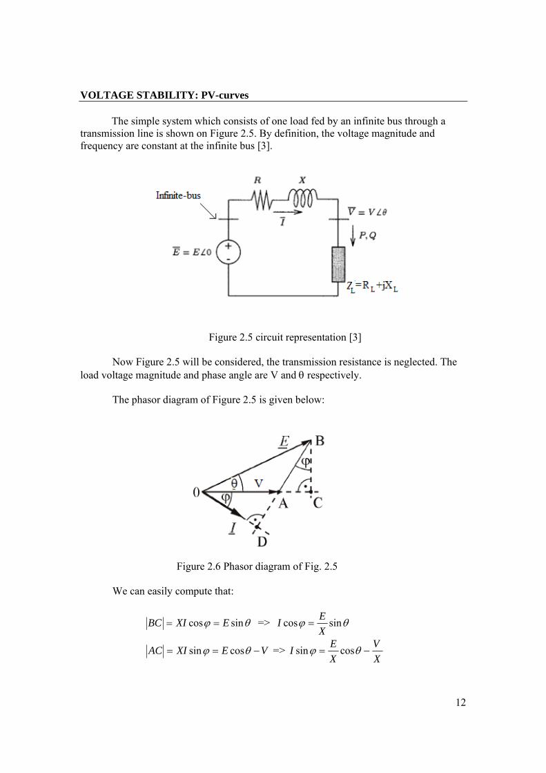
The simple system which consists of one load fed by an infinite bus through a
transmission line is shown on Figure 2.5. By definition, the voltage magnitude and frequency are constant at the infinite bus [3].
Figure 2.5 circuit representation [3]
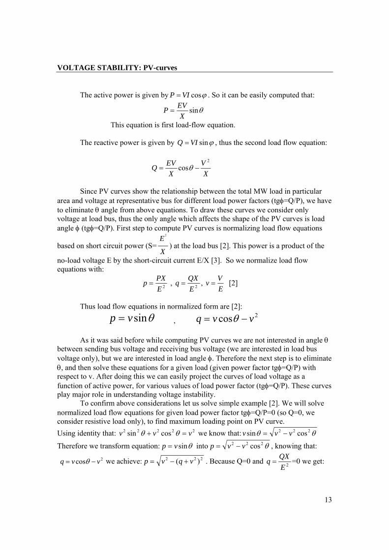
Now Figure 2.5 will be considered, the transmission resistance is neglected. The load voltage magnitude and phase angle are V and θ respectively. The phasor diagram of Figure 2.5 is given below:
Figure 2.6 Phasor diagram of Fig. 2.5 We can easily compute that:
θϕ sincos EXIBC == => θϕ sincosXEI =
VEXIAC −== θϕ cossin => XV
XEI −= θϕ cossin
VOLTAGE STABILITY: PV-curves
13
The active power is given by ϕcosVIP = . So it can be easily computed that:
θsinX
EVP =
This equation is first load-flow equation.
The reactive power is given by ϕsinVIQ = , thus the second load flow equation:
X
VX
EVQ2
cos −= θ
Since PV curves show the relationship between the total MW load in particular
area and voltage at representative bus for different load power factors (tgφ=Q/P), we have to eliminate θ angle from above equations. To draw these curves we consider only voltage at load bus, thus the only angle which affects the shape of the PV curves is load angle φ (tgφ=Q/P). First step to compute PV curves is normalizing load flow equations
based on short circuit power (S=X
E 2
) at the load bus [2]. This power is a product of the
no-load voltage E by the short-circuit current E/X [3]. So we normalize load flow equations with:
2EPXp = , 2E
QXq = , EVv = [2]
Thus load flow equations in normalized form are [2]:
θsinvp = , 2cos vvq −= θ
As it was said before while computing PV curves we are not interested in angle θ
between sending bus voltage and receiving bus voltage (we are interested in load bus voltage only), but we are interested in load angle φ. Therefore the next step is to eliminate θ, and then solve these equations for a given load (given power factor tgφ=Q/P) with respect to v. After doing this we can easily project the curves of load voltage as a function of active power, for various values of load power factor (tgφ=Q/P). These curves play major role in understanding voltage instability.
To confirm above considerations let us solve simple example [2]. We will solve normalized load flow equations for given load power factor tgφ=Q/P=0 (so Q=0, we consider resistive load only), to find maximum loading point on PV curve. Using identity that: 22222 cossin vvv =+ θθ we know that: θθ 222 cossin vvv −=
Therefore we transform equation: θsinvp = into θ222 cosvvp −= , knowing that:
2cos vvq −= θ we achieve: 222 )( vqvp +−= . Because Q=0 and 2EQXq = =0 we get:
VOLTAGE STABILITY: PV-curves
14
42 vvp −= . To find maximum loading point we have to find critical voltage corresponding to maximum power. We do it by taking a derivative (dp/dv)=0. Thus we
get: 0)42()(21 32/142 =−−= − vvvv
dvdp . We have two solutions: 0=v and
21
=v
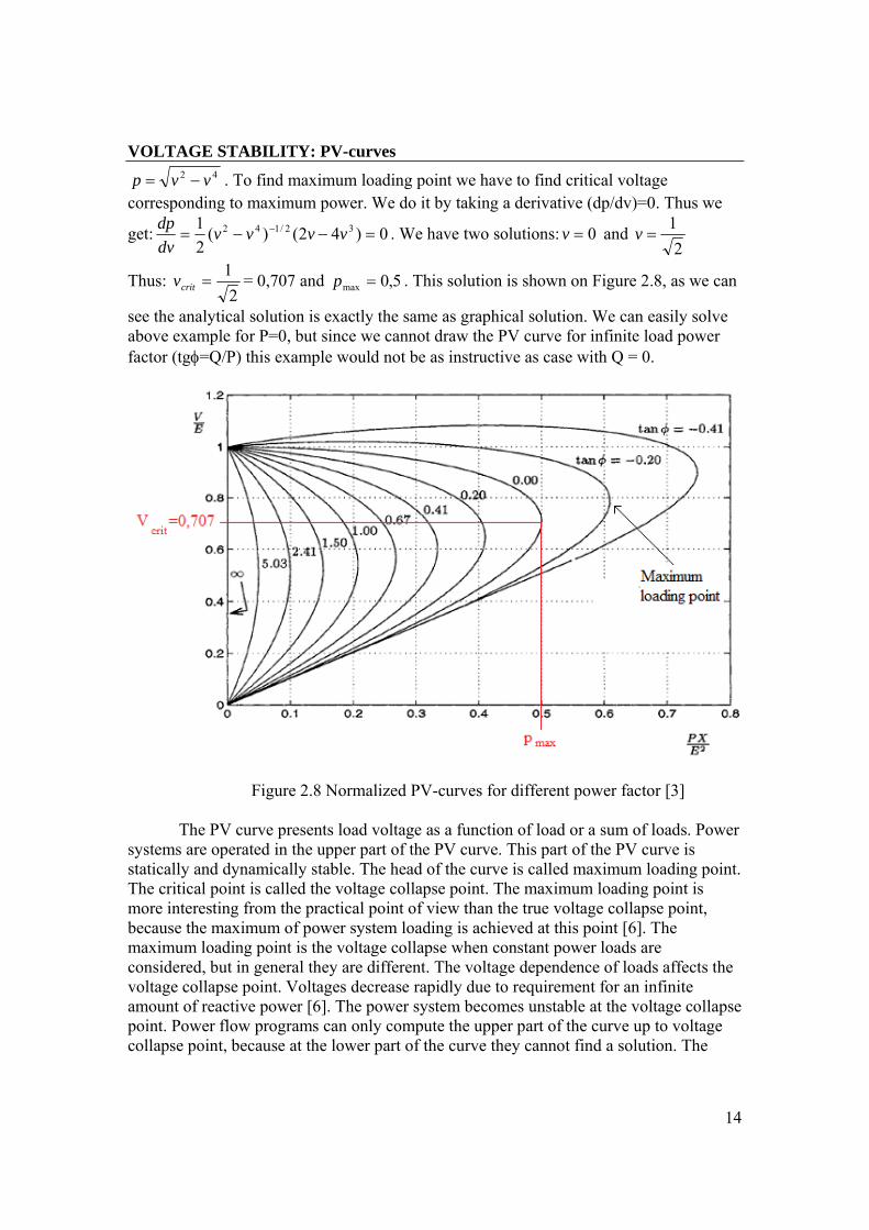
Thus: 2
1=critv = 0,707 and 5,0max =p . This solution is shown on Figure 2.8, as we can
see the analytical solution is exactly the same as graphical solution. We can easily solve above example for P=0, but since we cannot draw the PV curve for infinite load power factor (tgφ=Q/P) this example would not be as instructive as case with Q = 0.
Figure 2.8 Normalized PV-curves for different power factor [3]
The PV curve presents load voltage as a function of load or a sum of loads. Power
systems are operated in the upper part of the PV curve. This part of the PV curve is statically and dynamically stable. The head of the curve is called maximum loading point. The critical point is called the voltage collapse point. The maximum loading point is more interesting from the practical point of view than the true voltage collapse point, because the maximum of power system loading is achieved at this point [6]. The maximum loading point is the voltage collapse when constant power loads are considered, but in general they are different. The voltage dependence of loads affects the voltage collapse point. Voltages decrease rapidly due to requirement for an infinite amount of reactive power [6]. The power system becomes unstable at the voltage collapse point. Power flow programs can only compute the upper part of the curve up to voltage collapse point, because at the lower part of the curve they cannot find a solution. The
VOLTAGE STABILITY: PV-curves
15
iteration process is divergent below the voltage collapse point. Thus the whole computation in this project will be finished at voltage collapse point.
As the load is more and more compensated, which corresponds to smaller tanφ, maximum power increases and voltage increases as well. This situation is dangerous, because the maximum transfer capability may be reached at voltages close to normal operation values [3]. For overcompensated loads tanφ < 0, there is a portion of the upper PV curve along which the voltage increases with the load power [3].
Figure 2.8 presents PV curves for the system. These curves represent different load compensation cases (tanφ =Q/P). Since inductive line losses make it inefficient to supply a large amount of reactive power over long transmission lines, the reactive power loads must be supported locally [6]. According to figure 2.8 addition of the load compensation (decrement of the value of tanφ ) is beneficial for the power system. The load compensation makes it possible to increase the loading of the power system according to voltage stability. Thus, the monitoring of power system security becomes more complicated because critical voltage might be close to voltages of normal operation range [6].
The opportunity to increase power system loading by load and line compensation
is valuable nowadays. Compensation investments are usually less expensive and more environmental friendly than line investments. Furthermore, construction of new line has become time-consuming if not even impossible in some cases [6]. At the same time new generation plants are being constructed farther away from loads centers, fossil-fired power plants are being shut down in the cities and more electricity is being exported and imported. This trend inevitably requires addition of transmission capacity in the long run [6].
Although they are probably the most popular, the PV curves are not only possible projection of load-flow equations, which are solved for given load P, Q with respect to V and θ. We can similarly produce QV curves.
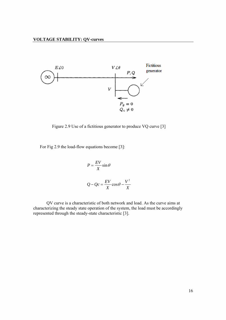
A QV curves expresses the relationship between the reactive support Qc at a given bus and the voltage at that bus. It can be determined by connecting a fictitious generator with zero active power and recording the reactive power Qc as the terminal voltage is being varied. Because, it does not produce the active power, the fictitious generator can be treated as a synchronous condenser. Since voltage is taken as an independent variable, it is common practice to use V as the abscissa and produce VQ instead of QV curves [3].
VOLTAGE STABILITY: QV-curves
16
Figure 2.9 Use of a fictitious generator to produce VQ curve [3]
For Fig 2.9 the load-flow equations become [3]:
XV
XEVQcQ
XEVP
2
cos
sin
−=−
=
θ
θ
QV curve is a characteristic of both network and load. As the curve aims at characterizing the steady state operation of the system, the load must be accordingly represented through the steady-state characteristic [3].
VOLTAGE STABILITY: QV-curves
17
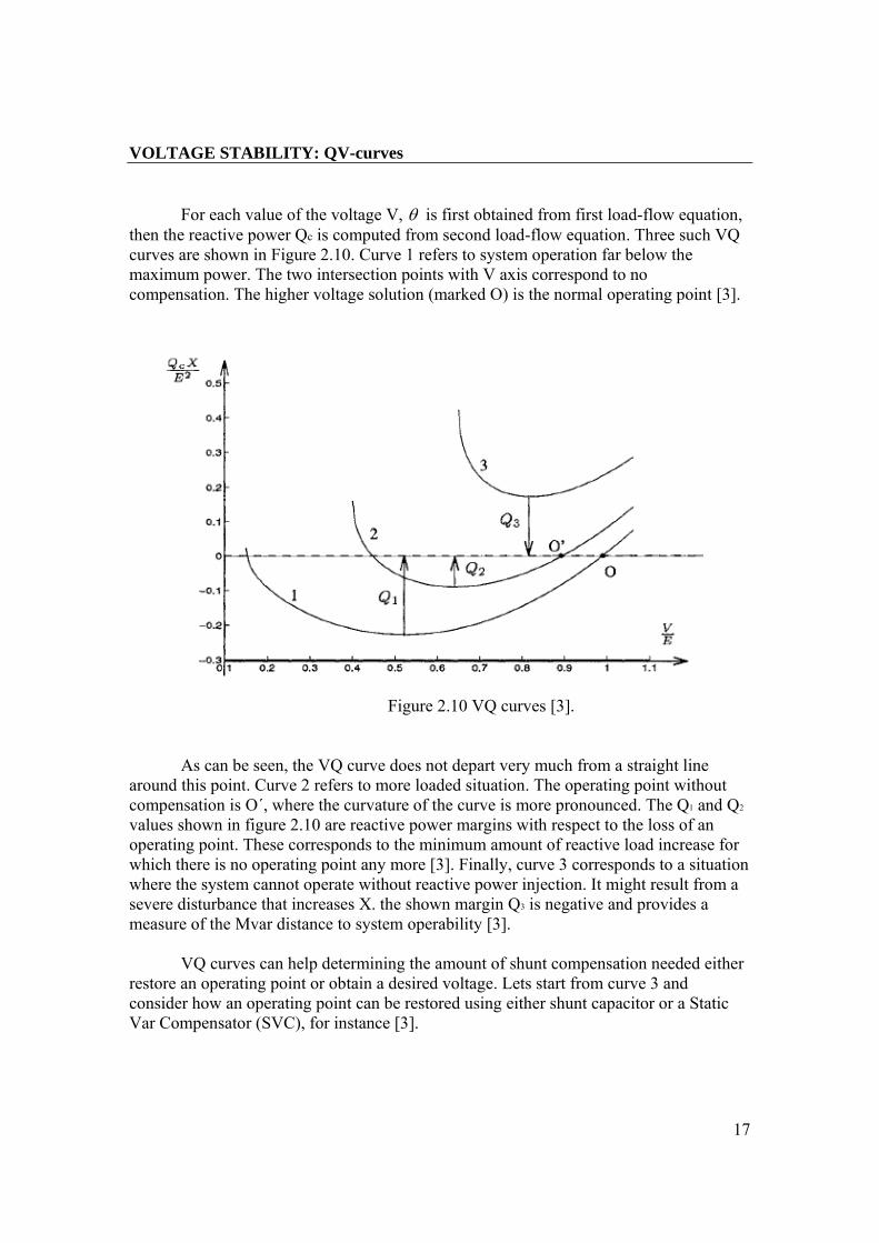
For each value of the voltage V, θ is first obtained from first load-flow equation, then the reactive power Qc is computed from second load-flow equation. Three such VQ curves are shown in Figure 2.10. Curve 1 refers to system operation far below the maximum power. The two intersection points with V axis correspond to no compensation. The higher voltage solution (marked O) is the normal operating point [3].
Figure 2.10 VQ curves [3].
As can be seen, the VQ curve does not depart very much from a straight line around this point. Curve 2 refers to more loaded situation. The operating point without compensation is O´, where the curvature of the curve is more pronounced. The Q1 and Q2 values shown in figure 2.10 are reactive power margins with respect to the loss of an operating point. These corresponds to the minimum amount of reactive load increase for which there is no operating point any more [3]. Finally, curve 3 corresponds to a situation where the system cannot operate without reactive power injection. It might result from a severe disturbance that increases X. the shown margin Q3 is negative and provides a measure of the Mvar distance to system operability [3].
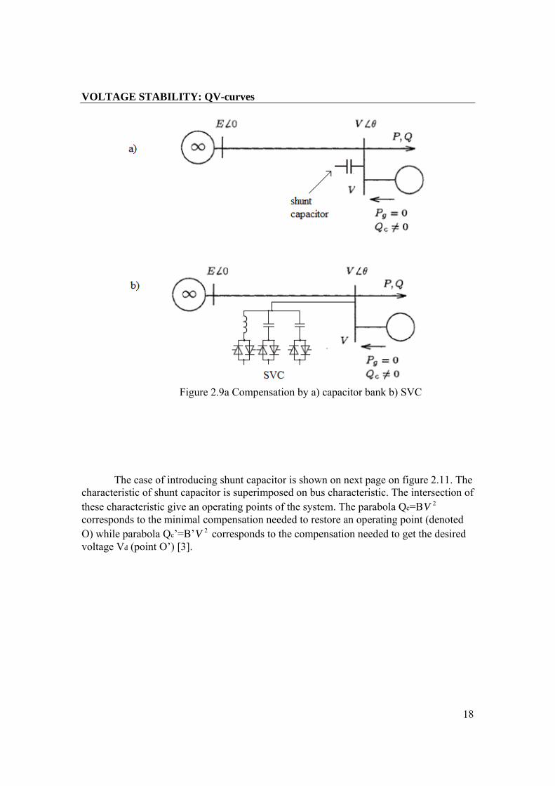
VQ curves can help determining the amount of shunt compensation needed either
restore an operating point or obtain a desired voltage. Lets start from curve 3 and consider how an operating point can be restored using either shunt capacitor or a Static Var Compensator (SVC), for instance [3].
VOLTAGE STABILITY: QV-curves
18
Figure 2.9a Compensation by a) capacitor bank b) SVC
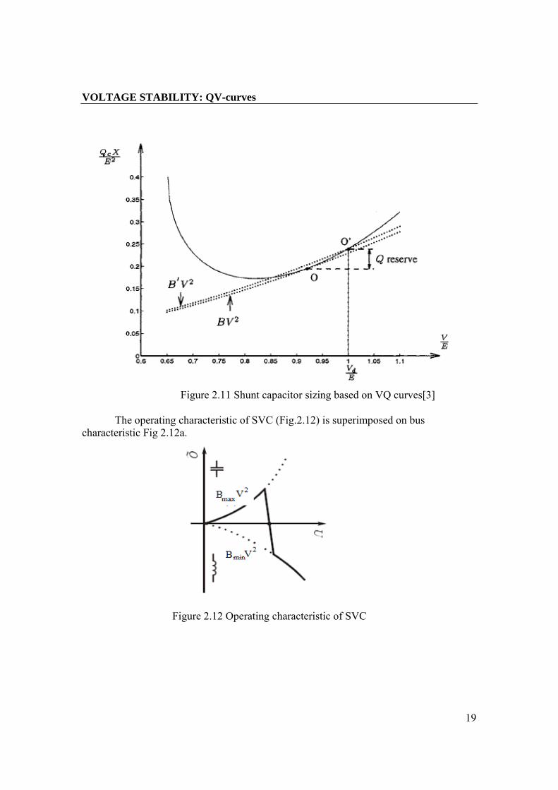
The case of introducing shunt capacitor is shown on next page on figure 2.11. The
characteristic of shunt capacitor is superimposed on bus characteristic. The intersection of these characteristic give an operating points of the system. The parabola Qc=B 2V corresponds to the minimal compensation needed to restore an operating point (denoted O) while parabola Qc’=B’ 2V corresponds to the compensation needed to get the desired voltage Vd (point O’) [3].
VOLTAGE STABILITY: QV-curves
19
Figure 2.11 Shunt capacitor sizing based on VQ curves[3] The operating characteristic of SVC (Fig.2.12) is superimposed on bus characteristic Fig 2.12a.
Figure 2.12 Operating characteristic of SVC
VOLTAGE STABILITY: QV-curves
20
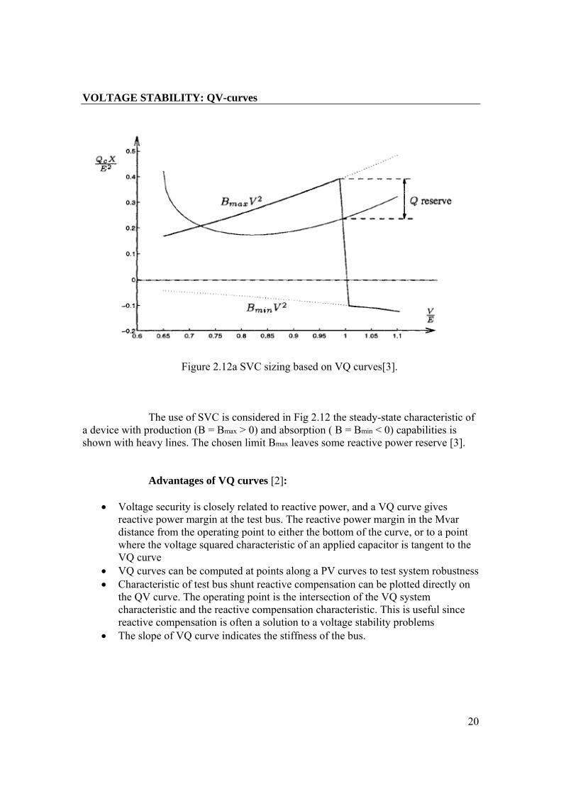
Figure 2.12a SVC sizing based on VQ curves[3]. The use of SVC is considered in Fig 2.12 the steady-state characteristic of a device with production (B = Bmax > 0) and absorption ( B = Bmin < 0) capabilities is shown with heavy lines. The chosen limit Bmax leaves some reactive power reserve [3]. Advantages of VQ curves [2]:
• Voltage security is closely related to reactive power, and a VQ curve gives reactive power margin at the test bus. The reactive power margin in the Mvar distance from the operating point to either the bottom of the curve, or to a point where the voltage squared characteristic of an applied capacitor is tangent to the VQ curve
• VQ curves can be computed at points along a PV curves to test system robustness • Characteristic of test bus shunt reactive compensation can be plotted directly on
the QV curve. The operating point is the intersection of the VQ system characteristic and the reactive compensation characteristic. This is useful since reactive compensation is often a solution to a voltage stability problems
• The slope of VQ curve indicates the stiffness of the bus.
VOLTAGE COLLAPSE
21
2.3.2 Voltage collapse
Voltage collapse is the process by which the sequence of events accompanying voltage instability leads to a low unacceptable voltage profile in a significant part of the power system. It can be manifested in several different ways [1].
When a power system is subjected to a sudden increase of reactive power demand
following a system contingency, the additional demand is met by the reactive power reserves carried by the generators and compensators. Usually there are sufficient reserves and the power system settles to a stable voltage level. However, it is possible, because of o combination of events and system conditions, that the additional reactive power demand may lead to voltage collapse causing to major brake down of part of the system [1].
The typical voltage collapse caused by long term stability is characterized as
follows [6] [1]: - Some extra high voltage (EHV) transmission lines are heavily loaded,
the available generation capacity of the critical area is temporarily reduced due to maintenance of unit or to market conditions, and reactive power reserves are at the minimum or are located far from the critical area
- Due to a fault or any other reason a heavily loaded line is lost. The loading and reactive power losses of remaining lines increases. The total reactive power demand increases due to these reasons.
- Immediately after the loss of EHV line, there would be reduction of voltage at adjacent load centers due to an extra reactive power demand. This would cause a load reduction, and resulting in reduction of power flow in remaining EHV lines and thus has a stabilizing effect. The voltage control of the system, however, quickly restores generator terminal voltages by increasing excitation. The additional reactive power flow at the transformers and transmission lines causes additional voltage drop at these components.
- The EHV level voltage reduction at load centers would be reflected into the distribution system. The on load tap changers of distribution substation transformer restore the distribution network voltages and loads to prefault levels. With each tap change operation, the resulting
VOLTAGE COLLAPSE
22
increment in load on EHV lines would increase the line loses, which would cause a grater drop in EHV levels.
- The increased reactive power demand increases the reactive output of generators. When the generator hits the reactive power limit, its terminal voltage decreases. Its share of reactive power demand is shifted to another generator further away from critical area. This will lead to cascading overloading of generators. Fewer generators are available for voltage control and they are located far from critical areas. The decreased voltage at the transmission system reduces the effectiveness of shunt capacitors.
The process will eventually lead to voltage collapse, possibly leading to loss of synchronism of generating units and a major blackout.
2.3.2.1 Examples of voltage collapse
France 1978 [2]: The load increment was 1600MW higher than
one at previous day between 7am and 8am. Voltages on the eastern 400 kV transmission network were between 342 and 347 kV at 8.20am. Low voltage reduced some thermal production and caused an overload relay tripping on major 400kV line at 8.26am. During restoration process another collapse occurred. Load interruption was 29GW and 100GWh. The restoration was finished at 12.30am.
Belgium 1982 [2]: A total collapse occurred in about four minutes due to the disconnection of a 700MW unit during commissioning test.
Southern Sweden 1983 [6]: The loss of a 400\220kV substation due to a fault caused cascading line outages and tripping of nuclear power units by over-current protection, which led to the isolation of Southern Sweden and total blackout in about one minute.
Florida USA 1985 [2]: A brush fire caused the tripping of 500kV lines and resulted in voltage collapse in a few seconds.
Western France 1987 [2]: Voltages decayed due to the tripping of four thermal units which resulted in the tripping of nine other thermal units and defect of eight unit over-excitation protection, thus voltages stabilized at a very low level 0,5-0,8 pu. After about six minutes of voltage collapse load shedding recovered the voltage.
VOLTAGE COLLAPSE
23
Southern Finland August 1992 [6]: The power system was
operated close to security limits. The import from Sweden was large, thus there were only three units directly connected to 400kV network in Southern Finland. The tripping of a 735MW generator unit, simultaneous maintenance work on 400kV line manual decrease of reactive power in another remaining unit caused a disturbance where the lowest voltage at a 400kV network was 344kV. The voltages restored to normal level about in 30 minutes by starting gas turbines, by some load shedding and by increasing reactive power production.
WSCC USA 1996 [6]: A short-circuit on a 345 kVline started a chain of events leading to a brake-up of the western North American power system. The final reason for the break-up was rapid overload/voltage collapse/angular instability.
Following chapter introduces basic principles of shunt compensation devices. It is basically a theoretical explanation of different shunt compensating equipment. After subsequent explanation, there will be a selection of particular shunt devices, which will be used in the experiments on improving voltage stability. The first part of this project is about steady state voltage stability, and the second part is about ways of improving it, thus it is necessary to understand how we can improve voltage stability and which kind of devices can be useful for this purpose. According to that, next chapter is very important part of this report, because it connects both theoretical parts in one harmonious whole. Therefore, the experiments on steady state voltage stability, which will be done in this project, will be easily understandable and no will have a problem to compare the results to theoretical basis.
REACTIVE POWER AND VOLTAGE CONTROL
24
3 REACTIVE POWER AND VOLTAGE CONTROL
3.1 INTRODUCTION
For efficient and reliable operation of power system, the control of voltage and reactive power should satisfy the following objectives [1]:
• Voltages at all terminals of all equipment in the system are within acceptable limits
• System stability is enhanced to maximize utilization of the transmission system
• The reactive power flow is minimized so as to reduce R 2I and X 2I losses. This ensures that the transmission system operates mainly for active power.
Thus the power system supplies power to a vast number of loads and is feeding from many generating units, there is a problem of maintaining voltages within required limits. As load varies, the reactive power requirements of the transmission system vary. Since the reactive power cannot be transferred over long distances, voltage control has to be effected by using special devices located through the system. The proper selection and coordination of equipment for controlling reactive power and voltage are among the major challenges of power system engineering [1].
3.2 Elements of the system, which are producing and absorbing
reactive power [1] Loads- a typical load bus supplied by a power system is composed of a large number of devices. The composition changes depending on the day, season and weather conditions. The composite characteristics are normally such that a load bus absorbs reactive power. Both active and reactive powers of the composite loads vary due to voltage magnitudes. Loads at low-lagging power factors cause excessive voltage drops in the transmission network. Industrial consumers are charged for reactive power and this convinces them to improve the load power factor. Underground cables- they are always loaded below their natural loads, and hence generate reactive power under all operating conditions Overhead lines- depending on the load current, either absorb or supply reactive power. At loads below the natural load, the lines produce net reactive power, on the contrary, at loads above natural load lines absorb reactive power.
WAYS OF IMPROVING VOLTAGE STABILITY
25
Synchronous generators- can generate or absorb reactive power depends on the excitation. When overexcited they supply reactive power, and when underexcited they absorb reactive power. Compensating devices- they installed in power system to either supply or absorb reactive power.
3.3 Ways of improving voltage stability and control
Reactive power compensation is often most effective way to improve both power transfer capability and voltage stability. The control of voltage levels is accomplished by controlling the production, absorption and flow of reactive power. The generating units provide the basic means of voltage control, because the automatic voltage regulators control field excitation to maintain scheduled voltage level at the terminals of the generators. To control voltage throughout the system we have to use addition devices to compensate reactive power [1]. Reactive compensation can be divided into series and shunt compensation. It can be also divided into active and passive compensation [2]. In next chapters of my work will be brief introduction of different solutions for improving system stability. But mostly consideration will be focused on shunt capacitor banks, static var compensator (SVC) and Static Synchronous Compensators (STATCOM), which are the part of group of active compensators called Flexible AC Transmission Systems (FACTS).
The devices used for these purposes may be classified as follows:
• Shunt capacitors
• Series capacitors
• Shunt reactors
• Synchronous condensers
• SVC
• STATCOM
Shunt capacitors and reactors and series capacitors provide passive compensation.
They are either permanently connected to the transmission and distribution system or switched. They contribute to voltage control by modifying the network characteristics. Synchronous condensers, SVC and STATCOM provide active compensation [2]. The
WAYS OF IMPROVING VOLTAGE STABILITY: SHUNT CAPACITORS
26
reactive power absorbed or supplied by them is automatically adjusted so as to maintain voltages of the buses to which they are connected. Together with the generating units, they establish voltages at specific points in the system. Voltages at other locations in the system are determined by active and reactive power flows through various elements, including the passive compensating devices [1].
3.3.2 SHUNT CAPACITORS
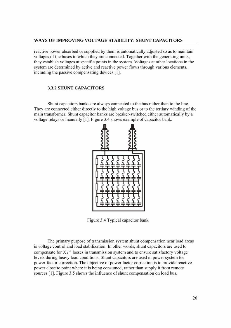
Shunt capacitors banks are always connected to the bus rather than to the line. They are connected either directly to the high voltage bus or to the tertiary winding of the main transformer. Shunt capacitor banks are breaker-switched either automatically by a voltage relays or manually [1]. Figure 3.4 shows example of capacitor bank.
Figure 3.4 Typical capacitor bank The primary purpose of transmission system shunt compensation near load areas
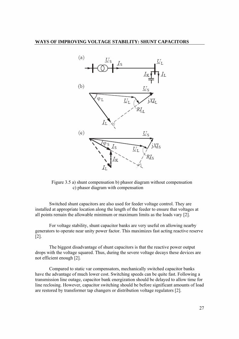
is voltage control and load stabilization. In other words, shunt capacitors are used to compensate for X 2I losses in transmission system and to ensure satisfactory voltage levels during heavy load conditions. Shunt capacitors are used in power system for power-factor correction. The objective of power factor correction is to provide reactive power close to point where it is being consumed, rather than supply it from remote sources [1]. Figure 3.5 shows the influence of shunt compensation on load bus.
WAYS OF IMPROVING VOLTAGE STABILITY: SHUNT CAPACITORS
27
Figure 3.5 a) shunt compensation b) phasor diagram without compensation c) phasor diagram with compensation Switched shunt capacitors are also used for feeder voltage control. They are
installed at appropriate location along the length of the feeder to ensure that voltages at all points remain the allowable minimum or maximum limits as the loads vary [2].
For voltage stability, shunt capacitor banks are very useful on allowing nearby generators to operate near unity power factor. This maximizes fast acting reactive reserve [2].
The biggest disadvantage of shunt capacitors is that the reactive power output drops with the voltage squared. Thus, during the severe voltage decays these devices are not efficient enough [2].
Compared to static var compensators, mechanically switched capacitor banks have the advantage of much lower cost. Switching speeds can be quite fast. Following a transmission line outage, capacitor bank energization should be delayed to allow time for line reclosing. However, capacitor switching should be before significant amounts of load are restored by transformer tap changers or distribution voltage regulators [2].
WAYS OF IMPROVING VOLTAGE STABILITY: SYNCHRONOUS CONDENSERS
28
Despite of many advantages of mechanically switched capacitors, there is couple of disadvantages as well. Firstly, for transient voltage instability, the switching may not be fast enough to prevent induction motor stalling. If voltage collapse results in system breakdown, the stable parts of the system may experience damaging overvoltages immediately following separation. Overvoltages would be aggravated by energizing of shunt capacitors during the period of voltage decay [2]. 3.3.3 SYNCHRONOUS CONDENSERS
Rotating synchronous condensers is fundamentally a synchronous motor that is attached to any driven equipment. It is started and connected to the electrical network as required to support a system’s voltage or to maintain the system power factor at specified level. The condenser’s installation and operation are identical to large electric motors.
A synchronous condenser provides a step less automatic power factor correction
with the ability to produce up 150% additional Mvars. Condensers can be installed inside or outside and are relatively small in size. The system produces no switching transients and is not affected by system electrical harmonics, some harmonics can even be absorbed by condensers. Condensers will not produce excessive voltage levels and are not susceptible to electrical resonances. Because of the rotating inertia of the condenser, it can provide voltage support even during a short power outage.
However, because of higher initial and operating costs, synchronous condensers
are generally not competitive with static var compensators. The capital cost may be 20-30% higher than SVCs. The full load losses of condensers are around 1.5% and no-load losses are around 1,5%. Synchronous condensers have couple advantages over SVC. They contribute to system short-circuit capability. The reactive power production is not affected by the system voltage. During power swings there is an exchange of kinetic energy between a synchronous condenser and the power system. During such swings, a synchronous condenser can supply a huge amount of reactive power. Unlike other form of shunt compensation it has an internal voltage source and is better able to cope with low system voltage conditions [1].
Recent applications of synchronous condensers have been mostly at HVDC
converter stations connected to the weak systems. They are used there to increase the network strength, by improving short-circuit capacity, and to improve commutation voltage [1].
WAYS OF IMPROVING VOLTAGE STABILITY: INTRODUCTION TO FACTS
29
3.3.4 INTRODUTCTION TO FACTS Chapters about reactive power compensation are based on references [4] [5]. The collective acronym FACTS has been adopted in recent years to describe a wide range of controllers, many of them incorporating large power electronic converters, which may, at present or in the future, used to increase the flexibility of power systems and thus make them more controllable [14]. Large interconnected systems develop too heavy loaded systems, especially if new lines can not be built because of lack of right-of-ways. Further, the location for new generation is often far away from the load and the system takes over also the task of transmitting power over longer distances. Due to the deregulation in electric power industry the requirements arise to transmit the power through given corridors. In some countries with remote power sources main problems result from requirement to transmit power over long distances through weak system leading to insufficient power quality. Problems resulting from above mentioned development may be at least partly economically improved by the use of Flexible AC Transmission System FACTS controllers [14]. FACTS have been defined as “alternating current transmission systems incorporating electronic-based and other static controllers to enhance controllability and increase power transfer capability” [14]. The fast development of power electronic in last two decades made it possible to design power electronic equipment of high rating for high voltage systems. Due to the fast control abilities of this equipment the operating conditions can be controlled in the system. This equipment are known as FACTS-Controller. The development of turn off devices e.g. GTO, IGTB, MCT for larger ratings opens a new possibility to build new more improved and sophisticated FACTS controllers [14]. FACTS controllers generally fall into two families: one comprises mainly the conventional thyristor-controlled SVC, TCSC and phase shifter, the other the converter-based STATCOM, static synchronous series compensator [SSSC], unified power flow controller [UPFC] and interline power flow controller [IPFC]. Although presently a large number of SVC installations exist, the converter based FACTS controllers like STATCOM clearly represent the future trend due to their superior performance and to their greater functional operating flexibility (which will be shown in following chapters) [4]. FACTS technology crates the following opportunities [14]:
• Control of power so that the desired amount of flows through the prescribed routes. This could be in the context of ownership, contract path, or to shift power away from overloaded lines.
• Secure loading of transmission lines near their steady state, short time and dynamic limits. Various contingency conditions can be accommodated to enhance the value off assets.
WAYS OF IMPROVING VOLTAGE STABILITY: INTRODUCTION TO FACTS
30
• Reduced generation and reserve margins through enhanced, secure
transmission interconnections for emergency power with neighboring utilities
• Contain cascading outages by limiting the impact of multiple faults leading to major blackouts.
• Undertake and effectively utilize upgrading of transmission lines by increasing voltage and/or current ratings. In a gross sense, the concept of building a higher voltage grid for accommodating future load growth is now modified in that, current upgrading is also a valid alternative.
Impact of controller location The shunt device operates by change of voltage and has its maximum impact on
power flow if located at the point of the transmission line where voltage is weakest. The location of the equipment has a significant impact on power flow control performance. Therefore, the best place for compensation in radial lines is the end of the line, where is the biggest variation of load. If we consider line which connects two system buses, the best place for compensation is the middle of the line.
3.3.4.1 Static Var Compensator SVC Static var compensators are shunt-connected static generators or/and absorbers
whose outputs are varied so as to control specific parameters of an electric power system. SVCs overcome the limitation of mechanically switched shunt capacitors or reactors. Advantages include fast, precise regulation of voltage and unrestricted, transient free capacitor switching. The basic elements of SVCs are capacitor banks or reactors in series with a bidirectional thyristors [1].
Basic types of SVCs: • Saturated reactor (SR) • Thyristor-controlled reactor (TCR) • Thyristor-switched capacitor (TSC) • Thyristor-switched reactor (TSR) • Thyristor control transformer (TCT) • Self- or line-commutated converter (SCC/LCC)
In subsequent chapters the most popular SVC devices will be presented and
different combination of these devices, which creates a Static Var System (SVS). Static var systems are capable of controlling individual phase voltages of the buses to which they are connected. Therefore they can be used for control of negative-sequence as well as positive-sequence of voltage deviations. But this issue will be discussed in the following chapters.

WAYS OF IMPROVING VOLTAGE STABILITY: TCR
31
3.3.4.1.1 The Thyristor-Controlled reactor TCR An elementary single-phase thyristor-controlled reactor TCR consists of fixed
reactor of inductance L, and a bidirectional thyristor valve [4].
Figure 3.10 thyristor-controlled reactor The thyristor conducts on alternate half cycles of the supply frequency depending
on the firing angle α. The magnitude of the current in the reactor can be varied continuously by this method of delay angle control form maximum (α=0) to zero at (α=90), as illustrated in the Figure 3.11. The adjustment of current in the reactor can take place only once in each half cycle, in the zero to 90 0 interval. This restriction results in a delay of attainable current control. The worst case delay, when changing the current from maximum to zero, is a half cycle of the applied voltage [4].
Figure 3.11 TCR operating waveforms [4] The amplitude IL(α) of the fundamental reactor current iL(α) can be expressed as a
function of angle α [4]:
WAYS OF IMPROVING VOLTAGE STABILITY: TCR
32
)2sin121()( ααω
αΠ
−Π
−=L
VI L
Where V is the amplitude of the applied ac voltage, L is the inductance of the
thyristor-controlled reactor, and ω is the angular frequency of the applied voltage. It is clear that the TCR can control the fundamental current continuously from zero (valve open) to a maximum (valve closed) as if it was a variable reactive admittance. Thus, an effective admittance, BL(α), can be defined as [4]:
)2sin121(1)( ααω
αΠ
−Π
−=L
BL
As we can see the admittance varies in the same manner as fundamental current.
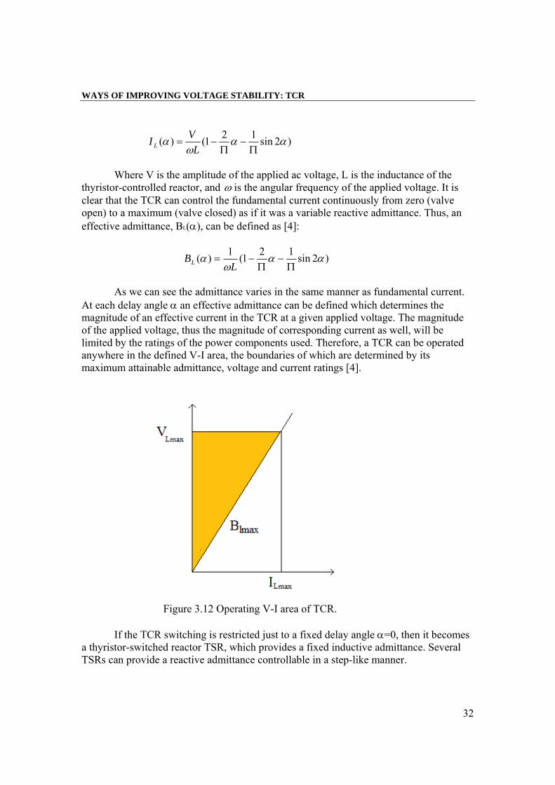
At each delay angle α an effective admittance can be defined which determines the magnitude of an effective current in the TCR at a given applied voltage. The magnitude of the applied voltage, thus the magnitude of corresponding current as well, will be limited by the ratings of the power components used. Therefore, a TCR can be operated anywhere in the defined V-I area, the boundaries of which are determined by its maximum attainable admittance, voltage and current ratings [4].
Figure 3.12 Operating V-I area of TCR. If the TCR switching is restricted just to a fixed delay angle α=0, then it becomes
a thyristor-switched reactor TSR, which provides a fixed inductive admittance. Several TSRs can provide a reactive admittance controllable in a step-like manner.
WAYS OF IMPROVING VOLTAGE STABILITY: TCR
33
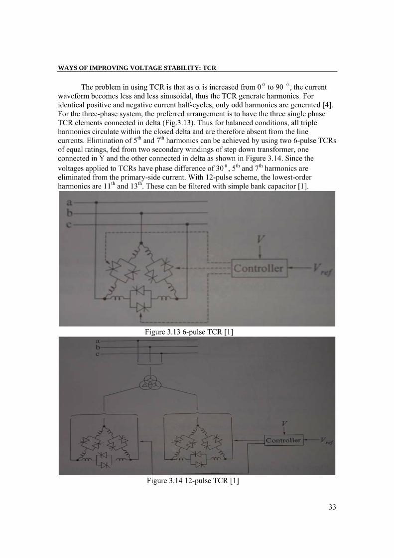
The problem in using TCR is that as α is increased from 0 0 to 90 0 , the current
waveform becomes less and less sinusoidal, thus the TCR generate harmonics. For identical positive and negative current half-cycles, only odd harmonics are generated [4]. For the three-phase system, the preferred arrangement is to have the three single phase TCR elements connected in delta (Fig.3.13). Thus for balanced conditions, all triple harmonics circulate within the closed delta and are therefore absent from the line currents. Elimination of 5th and 7th harmonics can be achieved by using two 6-pulse TCRs of equal ratings, fed from two secondary windings of step down transformer, one connected in Y and the other connected in delta as shown in Figure 3.14. Since the voltages applied to TCRs have phase difference of 30 0 , 5th and 7th harmonics are eliminated from the primary-side current. With 12-pulse scheme, the lowest-order harmonics are 11th and 13th. These can be filtered with simple bank capacitor [1].
Figure 3.13 6-pulse TCR [1]
Figure 3.14 12-pulse TCR [1]
WAYS OF IMPROVING VOLTAGE STABILITY: TSC
34
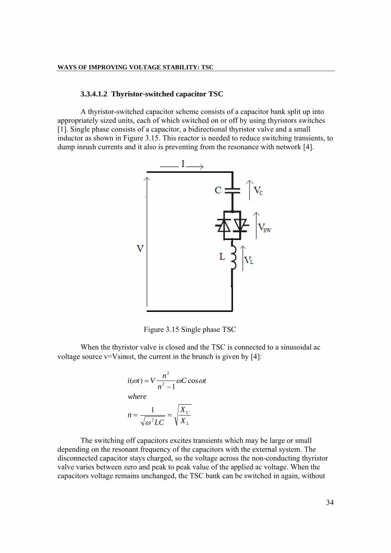
3.3.4.1.2 Thyristor-switched capacitor TSC A thyristor-switched capacitor scheme consists of a capacitor bank split up into
appropriately sized units, each of which switched on or off by using thyristors switches [1]. Single phase consists of a capacitor, a bidirectional thyristor valve and a small inductor as shown in Figure 3.15. This reactor is needed to reduce switching transients, to dump inrush currents and it also is preventing from the resonance with network [4].
Figure 3.15 Single phase TSC When the thyristor valve is closed and the TSC is connected to a sinusoidal ac
voltage source v=Vsinωt, the current in the brunch is given by [4]:
L
C
XX
LCn
where
tCn
nVti
==
−=
2
2
2
1
cos1
)(
ω
ωωω
The switching off capacitors excites transients which may be large or small
depending on the resonant frequency of the capacitors with the external system. The disconnected capacitor stays charged, so the voltage across the non-conducting thyristor valve varies between zero and peak to peak value of the applied ac voltage. When the capacitors voltage remains unchanged, the TSC bank can be switched in again, without
WAYS OF IMPROVING VOLTAGE STABILITY: TSC
35
any transient, at the appropriate peak voltage of the applied voltage. For positively charged capacitor the switching in is at positive peak of applied voltage, for negatively charged capacitor switching in is at negative peak of applied voltage. Usually, the capacitor bank is discharged after disconnection, therefore the reconnection can be done at some residual capacitor voltage [4].
The transient free conditions can be summarized as two simple rules. One, if the residual capacitor voltage is lower than the peak ac voltage, then the correct instant of switching is when the instantaneous ac voltage becomes equal to the capacitor voltage. Two, if the residual voltage of the capacitor is higher or equal to the peak ac voltage, then the correct switching is at the peak of ac voltage at which the thyristor valve voltage is minimum [4].
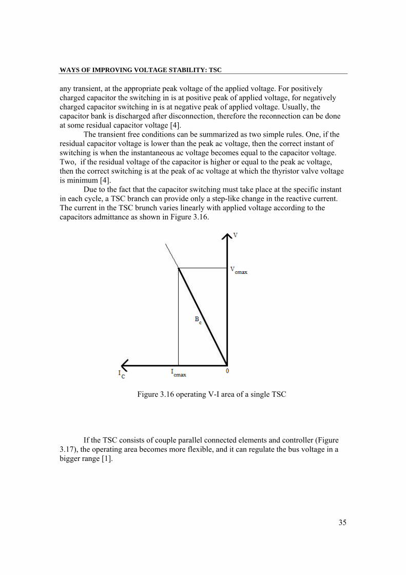
Due to the fact that the capacitor switching must take place at the specific instant in each cycle, a TSC branch can provide only a step-like change in the reactive current. The current in the TSC brunch varies linearly with applied voltage according to the capacitors admittance as shown in Figure 3.16.
Figure 3.16 operating V-I area of a single TSC If the TSC consists of couple parallel connected elements and controller (Figure
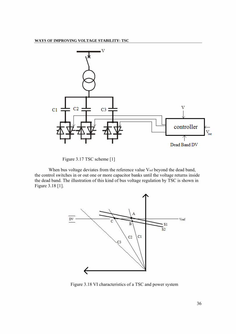
3.17), the operating area becomes more flexible, and it can regulate the bus voltage in a bigger range [1].
WAYS OF IMPROVING VOLTAGE STABILITY: TSC
36
Figure 3.17 TSC scheme [1] When bus voltage deviates from the reference value Vref beyond the dead band,
the control switches in or out one or more capacitor banks until the voltage returns inside the dead band. The illustration of this kind of bus voltage regulation by TSC is shown in Figure 3.18 [1].
Figure 3.18 VI characteristics of a TSC and power system
WAYS OF IMPROVING VOLTAGE STABILITY: FC-TCR
37
We can see that the voltage control is stepwise. It is determined by the rating and
number of parallel connected units. The bus voltage in this example is controlled within the range Vref (+/-)DV/2, where DV is dead band. When the system is operating so that its characteristic is S1, then capacitor C1 will be switched in and the operating point of the system will be in A [1]. If some fault happens, and system characteristic will change to S2 there will be a sudden bus voltage drop to the value represented by operating point B. The TSC control switches in bank C2 to change the operating point to C, and thus bringing the voltage within desired range. The time taken for executing a command from the controller ranges from half cycle to one cycle [1].
3.3.4.2 Static var systems SVS A static var compensation scheme with any desired control range can be formed
by using combinations of the elements described above. The SVS configuration depends on the different system requirements: the required speed of response, size range, flexibility, losses and costs.
In following chapter there will be description of different configuration of SVS which are facing different requirements of the system.
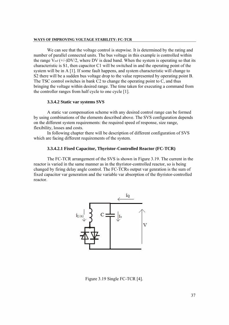
3.3.4.2.1 Fixed Capacitor, Thyristor-Controlled Reactor (FC-TCR) The FC-TCR arrangement of the SVS is shown in Figure 3.19. The current in the
reactor is varied in the same manner as in the thyristor-controlled reactor, so is being changed by firing delay angle control. The FC-TCRs output var genration is the sum of fixed capacitor var generation and the variable var absorption of the thyristor-controlled reactor.
Figure 3.19 Single FC-TCR [4].
WAYS OF IMPROVING VOLTAGE STABILITY: FC-TCR
38
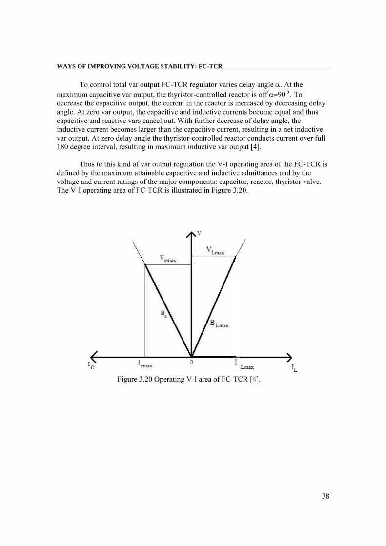
To control total var output FC-TCR regulator varies delay angle α. At the
maximum capacitive var output, the thyristor-controlled reactor is off α=90 0 . To decrease the capacitive output, the current in the reactor is increased by decreasing delay angle. At zero var output, the capacitive and inductive currents become equal and thus capacitive and reactive vars cancel out. With further decrease of delay angle, the inductive current becomes larger than the capacitive current, resulting in a net inductive var output. At zero delay angle the thyristor-controlled reactor conducts current over full 180 degree interval, resulting in maximum inductive var output [4].
Thus to this kind of var output regulation the V-I operating area of the FC-TCR is
defined by the maximum attainable capacitive and inductive admittances and by the voltage and current ratings of the major components: capacitor, reactor, thyristor valve. The V-I operating area of FC-TCR is illustrated in Figure 3.20.
Figure 3.20 Operating V-I area of FC-TCR [4].
WAYS OF IMPROVING VOLTAGE STABILITY: TSC-TCR
39
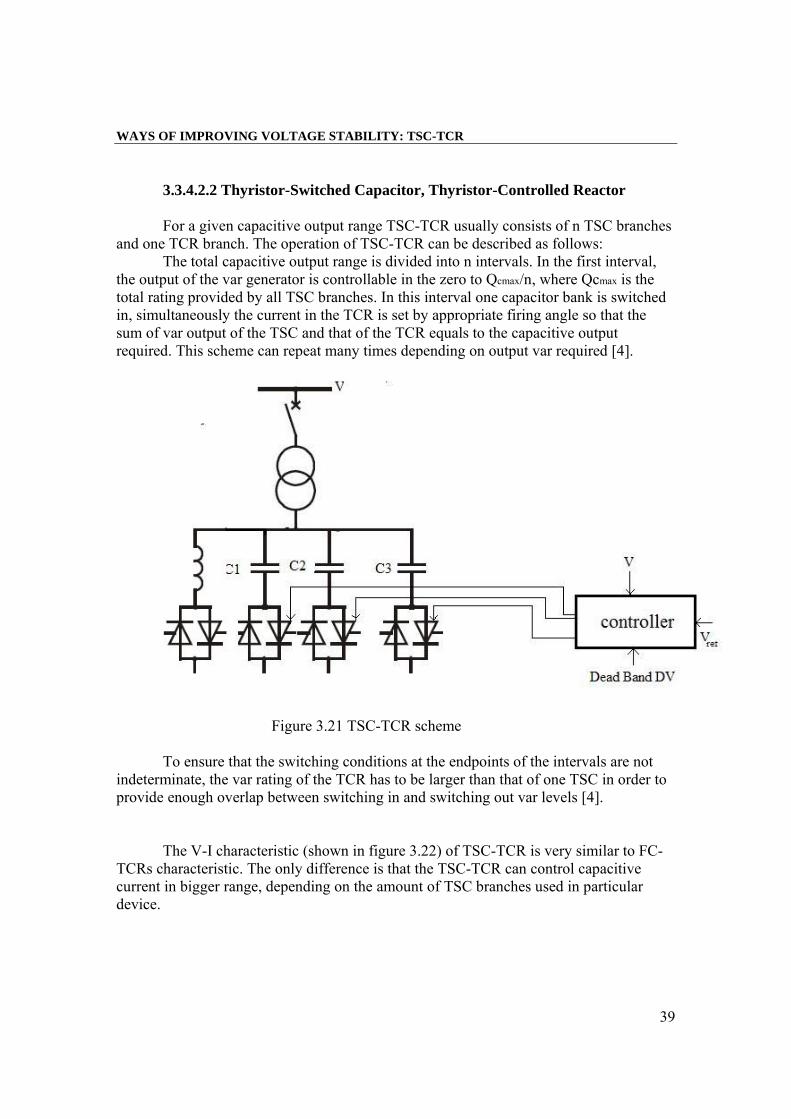
3.3.4.2.2 Thyristor-Switched Capacitor, Thyristor-Controlled Reactor For a given capacitive output range TSC-TCR usually consists of n TSC branches
and one TCR branch. The operation of TSC-TCR can be described as follows: The total capacitive output range is divided into n intervals. In the first interval,
the output of the var generator is controllable in the zero to Qcmax/n, where Qcmax is the total rating provided by all TSC branches. In this interval one capacitor bank is switched in, simultaneously the current in the TCR is set by appropriate firing angle so that the sum of var output of the TSC and that of the TCR equals to the capacitive output required. This scheme can repeat many times depending on output var required [4].
Figure 3.21 TSC-TCR scheme To ensure that the switching conditions at the endpoints of the intervals are not
indeterminate, the var rating of the TCR has to be larger than that of one TSC in order to provide enough overlap between switching in and switching out var levels [4].
The V-I characteristic (shown in figure 3.22) of TSC-TCR is very similar to FC-
TCRs characteristic. The only difference is that the TSC-TCR can control capacitive current in bigger range, depending on the amount of TSC branches used in particular device.

WAYS OF IMPROVING VOLTAGE STABILITY: TSC-TCR
40
Figure 3.22 Operating V-I area of the TSC-TCR The response of the TSC-TCR, depending on the number of TCR branches used.
The maximum switching delay in a single TSC, with a charged capacitor, is one cycle, whereas the, maximum switching delay of the TCR is only half of a cycle. However, if the TSC consists of more than two branches, there is high probability that one or more capacitor banks will be available with the charge of desired polarity [4].
Above described examples of SVS are treated recently as technically out of date
solutions, because of many limitation like for example, their performance depends on the ac system voltage. If some fault in the system causes big drop in voltage the SVS will not be able to react properly. This dependence is shown in Figure 3.23.
Figure 3.23 Static characteristic of SVS
WAYS OF IMPROVING VOLTAGE STABILITY: STATCOM
41
Devices, which performance does not depend on ac system voltage generate
reactive power directly, without the use of ac capacitors or reactors, by various switching of power converters. These devices are called Static Synchronous Compensators STATCOM. Following chapter will provide basic information about STATCOM.
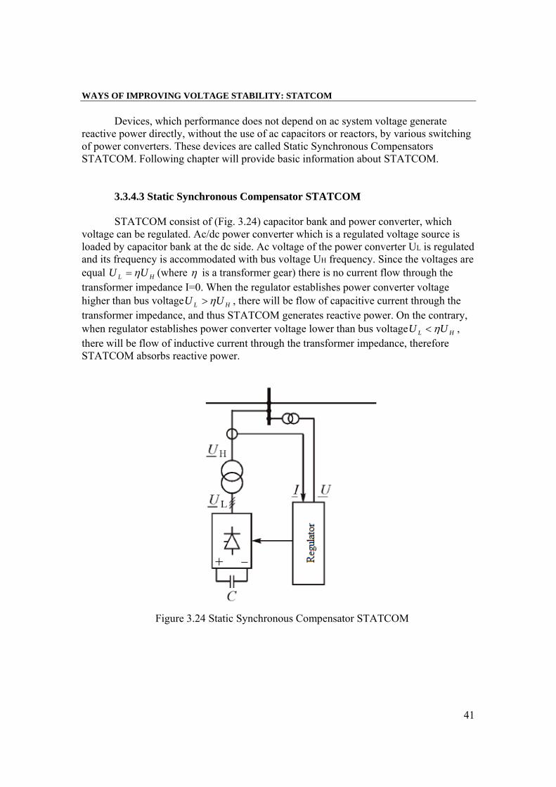
3.3.4.3 Static Synchronous Compensator STATCOM STATCOM consist of (Fig. 3.24) capacitor bank and power converter, which
voltage can be regulated. Ac/dc power converter which is a regulated voltage source is loaded by capacitor bank at the dc side. Ac voltage of the power converter UL is regulated and its frequency is accommodated with bus voltage UH frequency. Since the voltages are equal HL UU η= (where η is a transformer gear) there is no current flow through the transformer impedance I=0. When the regulator establishes power converter voltage higher than bus voltage HL UU η> , there will be flow of capacitive current through the transformer impedance, and thus STATCOM generates reactive power. On the contrary, when regulator establishes power converter voltage lower than bus voltage HL UU η< , there will be flow of inductive current through the transformer impedance, therefore STATCOM absorbs reactive power.
Figure 3.24 Static Synchronous Compensator STATCOM

WAYS OF IMPROVING VOLTAGE STABILITY: STATCOM
42
Above described compensator consists of capacitor bank only, but thanks to
power converter which voltage can be regulated, it can work as absorber or generator of reactive power.
Small size, lower costs and flexible regulation from capacitive range to inductive range are big advantages of STATCOM, which contribute to wider use of this kind of compensators in power system.
Figure 3.25 U-I operating area of STATCOM Figure 3.25 shows that the STATCOM can be operated over its full output current
range even at very low voltage, typically 0,2 p.u. system voltage levels. The maximum capacitive or inductive output current of the STATCOM can be maintained independently of the ac system voltage.
According to above chapters there are many of different devices which can improve voltage stability by injecting reactive power directly into load area. But in the researches only two of these devices will be investigated. First of them will be shunt capacitor bank which is used world wide. Shunt capacitor banks are usually installed at major substations in load area. The big advantage of shunt capacitor is much lower cost compared to other devices. It regulates the voltage in step manner and helps generators, which are close to operate with unity power factor and it allows keeping high level of fast acting reactive reserve.
Second device used in experiments is SVC, it was chosen because it is much cheaper than STATCOM and synchronous condensers and it is more often used all over the world. SVC gives a continuous and fast regulation of voltage, which is regulated according to the slope of SVC
SIMULATION OF GIVEN CASE
43
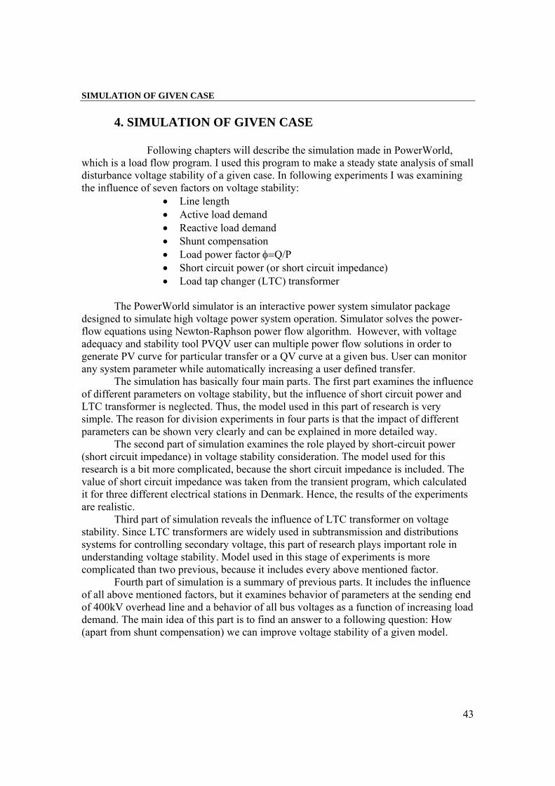
4. SIMULATION OF GIVEN CASE Following chapters will describe the simulation made in PowerWorld,
which is a load flow program. I used this program to make a steady state analysis of small disturbance voltage stability of a given case. In following experiments I was examining the influence of seven factors on voltage stability:
• Line length • Active load demand • Reactive load demand • Shunt compensation • Load power factor φ=Q/P • Short circuit power (or short circuit impedance) • Load tap changer (LTC) transformer
The PowerWorld simulator is an interactive power system simulator package designed to simulate high voltage power system operation. Simulator solves the power-flow equations using Newton-Raphson power flow algorithm. However, with voltage adequacy and stability tool PVQV user can multiple power flow solutions in order to generate PV curve for particular transfer or a QV curve at a given bus. User can monitor any system parameter while automatically increasing a user defined transfer.
The simulation has basically four main parts. The first part examines the influence of different parameters on voltage stability, but the influence of short circuit power and LTC transformer is neglected. Thus, the model used in this part of research is very simple. The reason for division experiments in four parts is that the impact of different parameters can be shown very clearly and can be explained in more detailed way.
The second part of simulation examines the role played by short-circuit power (short circuit impedance) in voltage stability consideration. The model used for this research is a bit more complicated, because the short circuit impedance is included. The value of short circuit impedance was taken from the transient program, which calculated it for three different electrical stations in Denmark. Hence, the results of the experiments are realistic.
Third part of simulation reveals the influence of LTC transformer on voltage stability. Since LTC transformers are widely used in subtransmission and distributions systems for controlling secondary voltage, this part of research plays important role in understanding voltage stability. Model used in this stage of experiments is more complicated than two previous, because it includes every above mentioned factor.
Fourth part of simulation is a summary of previous parts. It includes the influence of all above mentioned factors, but it examines behavior of parameters at the sending end of 400kV overhead line and a behavior of all bus voltages as a function of increasing load demand. The main idea of this part is to find an answer to a following question: How (apart from shunt compensation) we can improve voltage stability of a given model.
SIMULATION OF GIVEN CASE
44
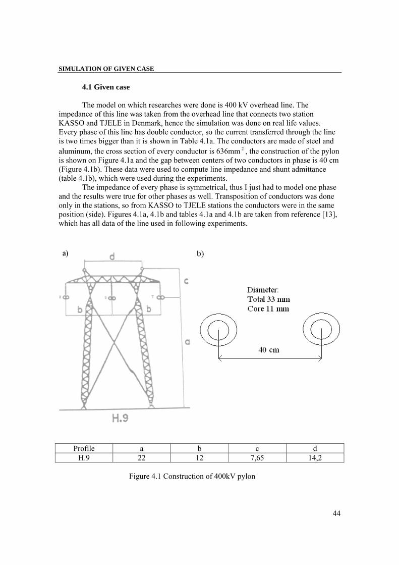
4.1 Given case The model on which researches were done is 400 kV overhead line. The
impedance of this line was taken from the overhead line that connects two station KASSO and TJELE in Denmark, hence the simulation was done on real life values. Every phase of this line has double conductor, so the current transferred through the line is two times bigger than it is shown in Table 4.1a. The conductors are made of steel and aluminum, the cross section of every conductor is 636mm 2 , the construction of the pylon is shown on Figure 4.1a and the gap between centers of two conductors in phase is 40 cm (Figure 4.1b). These data were used to compute line impedance and shunt admittance (table 4.1b), which were used during the experiments.
The impedance of every phase is symmetrical, thus I just had to model one phase and the results were true for other phases as well. Transposition of conductors was done only in the stations, so from KASSO to TJELE stations the conductors were in the same position (side). Figures 4.1a, 4.1b and tables 4.1a and 4.1b are taken from reference [13], which has all data of the line used in following experiments.
Profile a b c d H.9 22 12 7,65 14,2 Figure 4.1 Construction of 400kV pylon
SIMULATION OF GIVEN CASE
45
Thermal limits for current [A] in ambient temperature 20 0 C Conductor
temperature 50 0 C 65 0 C 80 0 C
Conductor type: 636 mm 2 FINCH
800 1036 1217
Table 4.1a Current thermal limits for 400 kV overhead line [13] Experiments will be performed for the conductor temperature 50 0 C. Parameters for this conditions are shown in Table 4.1b, current limit in table 4.1b is twice bigger than shown in Table 4.1a, because line has two conductors per phase.
Un [kV] R’ [Ω/km] X’ [Ω/km] B [μS/km] I limit [kA] 400 0,027 0,333 3,429 1,6
Table 4.1b parameters of overhead line used in experiments [13]
The modeling of above described 400 kV overhead line was done in PowerWorld simulator. Station in generation area was treated as a constant voltage and angle bus and the station in load area was treated as a load bus. Power transfer was modeled from generation area to load area through the impedance and admittance of above mentioned line. To investigate voltage stability I observed the behavior of bus voltage magnitude in the load area.
In PowerWorld the modeling of different line length can not be done directly, thus
to do that I was changing the impedance and admittance given in table 4.1 according to the line length. To model a change in power transfer I was changing load demand in the load area and according to this generation was being changed, thus power transmitted through tested line changed as well. Thanks to this I was able to observe behavior of bus voltage magnitude in the load area.
Next part of this paper shows the results of above mentioned experiments. As it
was said before the experiments have four main parts. In the first part the impact of short circuit power (short circuit impedance) and LTC transformer is excluded, but it is examined very deeply in the second and third part of research.

SIMULATION OF GIVEN CASE: PART 1
46
4.2 Part 1 Figure 4.1.1 illustrates a simple model of 400 kV overhead line connecting two
Danish stations. As it can be easily seen the short circuit impedance is not considered in this part of experiments. During first part of researches investigating of steady state small disturbance voltage stability is focused on such factors as:
Line length
Active load demand
Reactive load demand
Load power factor φ=Q/P
Shunt compensation
Figure 4.1.1 model of 400kV overhead line connecting generator bus and load bus.

SIMULATION OF GIVEN CASE: PART 1 results
47
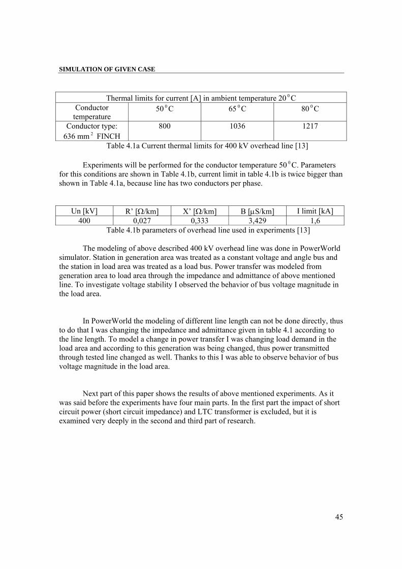
4.2.1 The influence of line length on voltage stability In this part of experiments the variable was line length and other parameters were
constant (load active and reactive power, no shunt compensation). The idea of this research was to check what is the influence of the line length on load bus voltages, while the load demand is constant. What is the maximum line length with given load, which in this case is 500 MW. Following table and plots show the results of above mentioned experiments.
Table 4.2 Results length
km line MW line Mvar
bus Voltage
pu load MW
load Mvar
MW losses
Mvar losses
I begin A I end A angle
50 500,12 -1,09 1 500 0 0,12 -1,09 724,75 724,71 -3
100 504,29 -1,05 0,99 500 0 4,29 -1,05 727,88 727,78 -6,04
150 506,49 -1,21 0,99 500 0 6,49 -1,21 731,06 730,97 -9,12
200 508,73 -0,15 0,98 500 0 8,73 -0,15 734,28 734,36 -12,2
250 511 1,85 0,98 500 0 11 1,85 737,57 738,14 -15,4
300 513,35 5 0,97 500 0 13,35 5 740,99 742,53 -18,6
350 515,77 9,72 0,97 500 0 15,77 9,72 744,88 747,87 -21,6
400 518,31 16,69 0,96 500 0 18,31 16,69 748,5 754,74 -25,4
425 519,62 21,46 0,95 500 0 19,62 21,46 750,65 759,08 -27,0
450 521 27,44 0,94 500 0 21 27,44 753,05 764,35 -29,0
480 522,77 36,98 0,93 500 0 22,77 36,98 756,44 772,49 -31,4
500 524,09 45,67 0,93 500 0 24,09 45,67 759,33 779,78 -33,1
510 524,8 51,04 0,92 500 0 24,8 51,04 761,06 784,24 -34
520 525,56 57,44 0,91 500 0 25,56 57,44 763,1 789,54 -34,9
530 526,4 65,15 0,91 500 0 26,4 65,15 765,59 795,95 -35,9
540 527,36 74,93 0,9 500 0 27,36 74,93 768,82 804,8 -37,1
550 528,46 87,95 0,89 500 0 28,46 87,95 773,26 814,93 -38,4
555 529,12 96,62 0,88 500 0 29,12 96,62 776,34 822,19 -39,2
560 529,99 108,42 0,87 500 0 29,99 108,42 780,81 832,15 -40,1
562 530,34 113,76 0,86 500 0 30,34 113,76 782,89 836,67 -40,5
564 520,79 120,67 0,86 500 0 20,79 120,67 785,68 842,55 -41,0
566 531,53 131,92 0,85 500 0 31,53 131,92 790,48 852,21 -41,4
SIMULATION OF GIVEN CASE: PART 1 results
48
Figure 4.2 The influence of line length on bus voltage
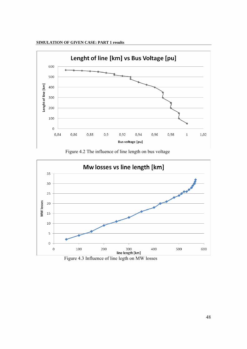
Figure 4.3 Influence of line legth on MW losses
SIMULATION OF GIVEN CASE: PART 1 results
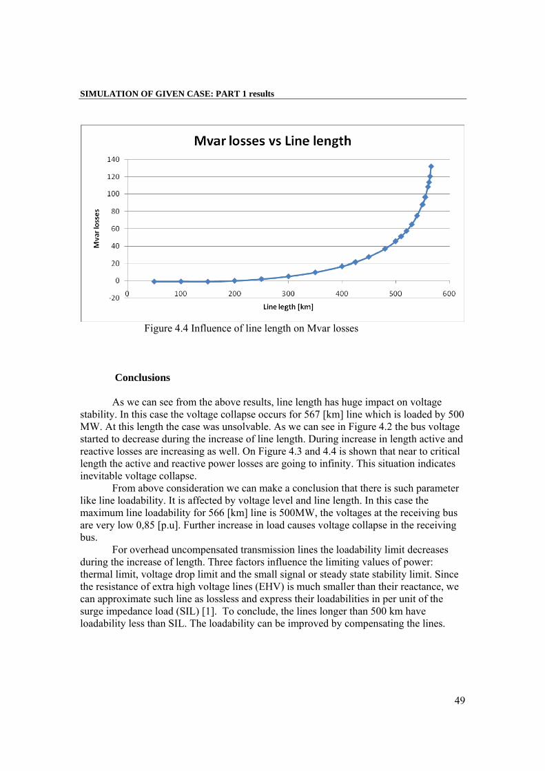
49
Figure 4.4 Influence of line length on Mvar losses Conclusions As we can see from the above results, line length has huge impact on voltage stability. In this case the voltage collapse occurs for 567 [km] line which is loaded by 500 MW. At this length the case was unsolvable. As we can see in Figure 4.2 the bus voltage started to decrease during the increase of line length. During increase in length active and reactive losses are increasing as well. On Figure 4.3 and 4.4 is shown that near to critical length the active and reactive power losses are going to infinity. This situation indicates inevitable voltage collapse. From above consideration we can make a conclusion that there is such parameter like line loadability. It is affected by voltage level and line length. In this case the maximum line loadability for 566 [km] line is 500MW, the voltages at the receiving bus are very low 0,85 [p.u]. Further increase in load causes voltage collapse in the receiving bus. For overhead uncompensated transmission lines the loadability limit decreases during the increase of length. Three factors influence the limiting values of power: thermal limit, voltage drop limit and the small signal or steady state stability limit. Since the resistance of extra high voltage lines (EHV) is much smaller than their reactance, we can approximate such line as lossless and express their loadabilities in per unit of the surge impedance load (SIL) [1]. To conclude, the lines longer than 500 km have loadability less than SIL. The loadability can be improved by compensating the lines.
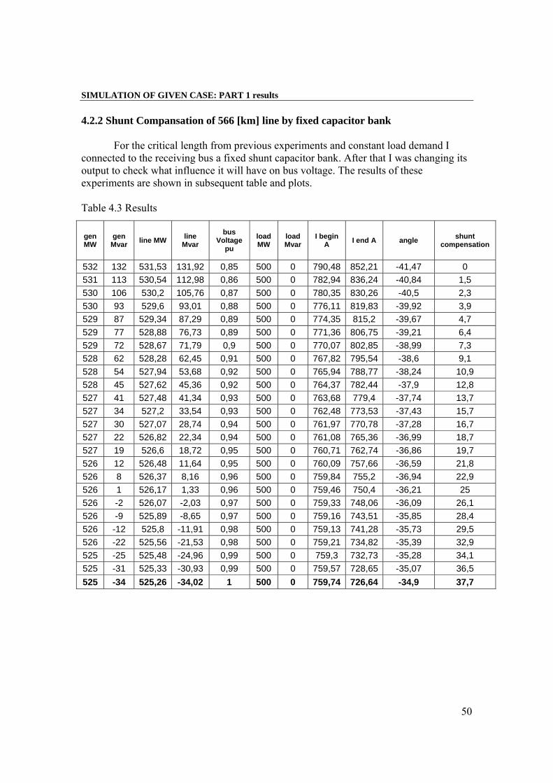
SIMULATION OF GIVEN CASE: PART 1 results
50
4.2.2 Shunt Compansation of 566 [km] line by fixed capacitor bank For the critical length from previous experiments and constant load demand I connected to the receiving bus a fixed shunt capacitor bank. After that I was changing its output to check what influence it will have on bus voltage. The results of these experiments are shown in subsequent table and plots. Table 4.3 Results
gen MW
gen Mvar line MW line
Mvar bus
Voltage pu
load MW
load Mvar
I begin A I end A angle shunt
compensation
532 132 531,53 131,92 0,85 500 0 790,48 852,21 -41,47 0 531 113 530,54 112,98 0,86 500 0 782,94 836,24 -40,84 1,5 530 106 530,2 105,76 0,87 500 0 780,35 830,26 -40,5 2,3 530 93 529,6 93,01 0,88 500 0 776,11 819,83 -39,92 3,9 529 87 529,34 87,29 0,89 500 0 774,35 815,2 -39,67 4,7 529 77 528,88 76,73 0,89 500 0 771,36 806,75 -39,21 6,4 529 72 528,67 71,79 0,9 500 0 770,07 802,85 -38,99 7,3 528 62 528,28 62,45 0,91 500 0 767,82 795,54 -38,6 9,1 528 54 527,94 53,68 0,92 500 0 765,94 788,77 -38,24 10,9 528 45 527,62 45,36 0,92 500 0 764,37 782,44 -37,9 12,8 527 41 527,48 41,34 0,93 500 0 763,68 779,4 -37,74 13,7 527 34 527,2 33,54 0,93 500 0 762,48 773,53 -37,43 15,7 527 30 527,07 28,74 0,94 500 0 761,97 770,78 -37,28 16,7 527 22 526,82 22,34 0,94 500 0 761,08 765,36 -36,99 18,7 527 19 526,6 18,72 0,95 500 0 760,71 762,74 -36,86 19,7 526 12 526,48 11,64 0,95 500 0 760,09 757,66 -36,59 21,8 526 8 526,37 8,16 0,96 500 0 759,84 755,2 -36,94 22,9 526 1 526,17 1,33 0,96 500 0 759,46 750,4 -36,21 25 526 -2 526,07 -2,03 0,97 500 0 759,33 748,06 -36,09 26,1 526 -9 525,89 -8,65 0,97 500 0 759,16 743,51 -35,85 28,4 526 -12 525,8 -11,91 0,98 500 0 759,13 741,28 -35,73 29,5 526 -22 525,56 -21,53 0,98 500 0 759,21 734,82 -35,39 32,9 525 -25 525,48 -24,96 0,99 500 0 759,3 732,73 -35,28 34,1 525 -31 525,33 -30,93 0,99 500 0 759,57 728,65 -35,07 36,5 525 -34 525,26 -34,02 1 500 0 759,74 726,64 -34,9 37,7
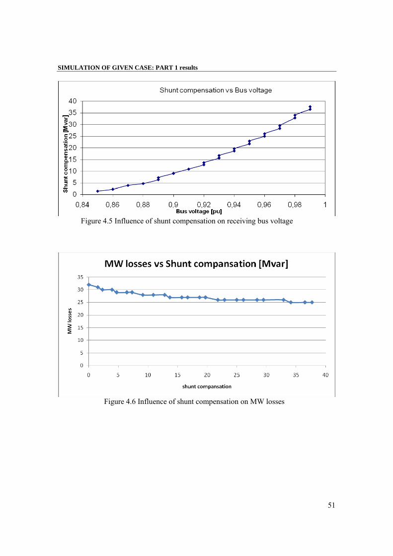
SIMULATION OF GIVEN CASE: PART 1 results
51
Figure 4.5 Influence of shunt compensation on receiving bus voltage
Figure 4.6 Influence of shunt compensation on MW losses
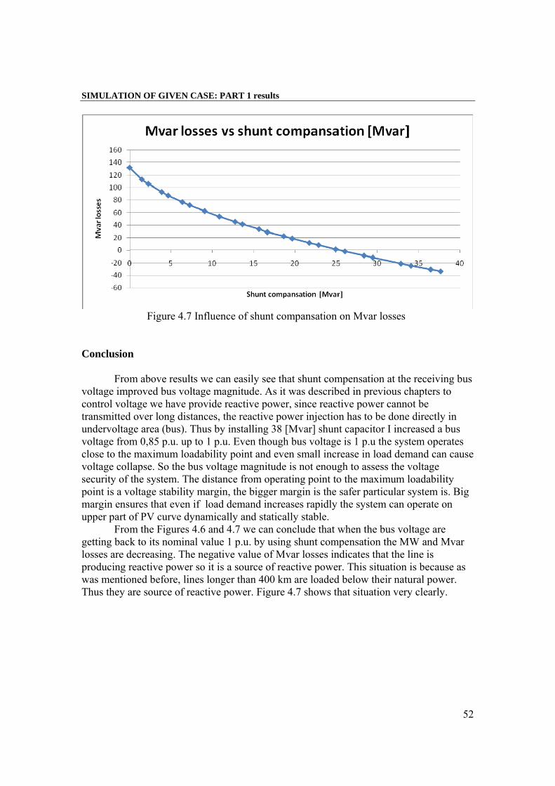
SIMULATION OF GIVEN CASE: PART 1 results
52
Figure 4.7 Influence of shunt compansation on Mvar losses Conclusion From above results we can easily see that shunt compensation at the receiving bus voltage improved bus voltage magnitude. As it was described in previous chapters to control voltage we have provide reactive power, since reactive power cannot be transmitted over long distances, the reactive power injection has to be done directly in undervoltage area (bus). Thus by installing 38 [Mvar] shunt capacitor I increased a bus voltage from 0,85 p.u. up to 1 p.u. Even though bus voltage is 1 p.u the system operates close to the maximum loadability point and even small increase in load demand can cause voltage collapse. So the bus voltage magnitude is not enough to assess the voltage security of the system. The distance from operating point to the maximum loadability point is a voltage stability margin, the bigger margin is the safer particular system is. Big margin ensures that even if load demand increases rapidly the system can operate on upper part of PV curve dynamically and statically stable. From the Figures 4.6 and 4.7 we can conclude that when the bus voltage are getting back to its nominal value 1 p.u. by using shunt compensation the MW and Mvar losses are decreasing. The negative value of Mvar losses indicates that the line is producing reactive power so it is a source of reactive power. This situation is because as was mentioned before, lines longer than 400 km are loaded below their natural power. Thus they are source of reactive power. Figure 4.7 shows that situation very clearly.
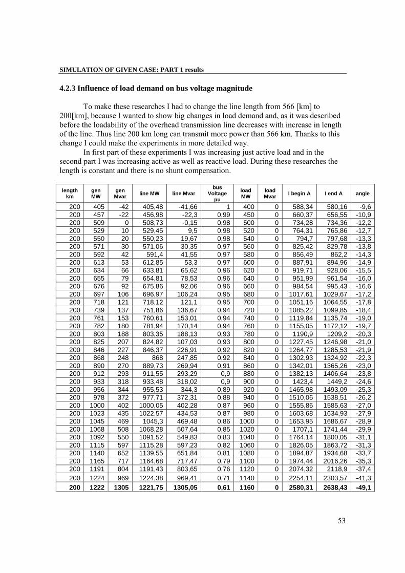
SIMULATION OF GIVEN CASE: PART 1 results
53
4.2.3 Influence of load demand on bus voltage magnitude To make these researches I had to change the line length from 566 [km] to 200[km], because I wanted to show big changes in load demand and, as it was described before the loadability of the overhead transmission line decreases with increase in length of the line. Thus line 200 km long can transmit more power than 566 km. Thanks to this change I could make the experiments in more detailed way. In first part of these experiments I was increasing just active load and in the second part I was increasing active as well as reactive load. During these researches the length is constant and there is no shunt compensation. length
km gen MW
gen Mvar line MW line Mvar
bus Voltage
pu load MW
load Mvar I begin A I end A angle
200 405 -42 405,48 -41,66 1 400 0 588,34 580,16 -9,6200 457 -22 456,98 -22,3 0,99 450 0 660,37 656,55 -10,9200 509 0 508,73 -0,15 0,98 500 0 734,28 734,36 -12,2200 529 10 529,45 9,5 0,98 520 0 764,31 765,86 -12,7200 550 20 550,23 19,67 0,98 540 0 794,7 797,68 -13,3200 571 30 571,06 30,35 0,97 560 0 825,42 829,78 -13,8200 592 42 591,4 41,55 0,97 580 0 856,49 862,2 -14,3200 613 53 612,85 53,3 0,97 600 0 887,91 894,96 -14,9200 634 66 633,81 65,62 0,96 620 0 919,71 928,06 -15,5200 655 79 654,81 78,53 0,96 640 0 951,99 961,54 -16,0200 676 92 675,86 92,06 0,96 660 0 984,54 995,43 -16,6200 697 106 696,97 106,24 0,95 680 0 1017,61 1029,67 -17,2200 718 121 718,12 121,1 0,95 700 0 1051,16 1064,55 -17,8200 739 137 751,86 136,67 0,94 720 0 1085,22 1099,85 -18,4200 761 153 760,61 153,01 0,94 740 0 1119,84 1135,74 -19,0200 782 180 781,94 170,14 0,94 760 0 1155,05 1172,12 -19,7200 803 188 803,35 188,13 0,93 780 0 1190,9 1209,2 -20,3200 825 207 824,82 107,03 0,93 800 0 1227,45 1246,98 -21,0200 846 227 846,37 226,91 0,92 820 0 1264,77 1285,53 -21,9200 868 248 868 247,85 0,92 840 0 1302,93 1324,92 -22,3200 890 270 889,73 269,94 0,91 860 0 1342,01 1365,26 -23,0200 912 293 911,55 293,29 0,9 880 0 1382,13 1406,64 -23,8200 933 318 933,48 318,02 0,9 900 0 1423,4 1449,2 -24,6200 956 344 955,53 344,3 0,89 920 0 1465,98 1493,09 -25,3200 978 372 977,71 372,31 0,88 940 0 1510,06 1538,51 -26,2200 1000 402 1000,05 402,28 0,87 960 0 1555,86 1585,63 -27,0200 1023 435 1022,57 434,53 0,87 980 0 1603,68 1634,93 -27,9200 1045 469 1045,3 469,48 0,86 1000 0 1653,95 1686,67 -28,9200 1068 508 1068,28 507,64 0,85 1020 0 1707,1 1741,44 -29,9200 1092 550 1091,52 549,83 0,83 1040 0 1764,14 1800,05 -31,1200 1115 597 1115,28 597,23 0,82 1060 0 1826,05 1863,72 -31,3200 1140 652 1139,55 651,84 0,81 1080 0 1894,87 1934,68 -33,7200 1165 717 1164,68 717,47 0,79 1100 0 1974,44 2016,26 -35,3200 1191 804 1191,43 803,65 0,76 1120 0 2074,32 2118,9 -37,4200 1224 969 1224,38 969,41 0,71 1140 0 2254,11 2303,57 -41,3200 1222 1305 1221,75 1305,05 0,61 1160 0 2580,31 2638,43 -49,1
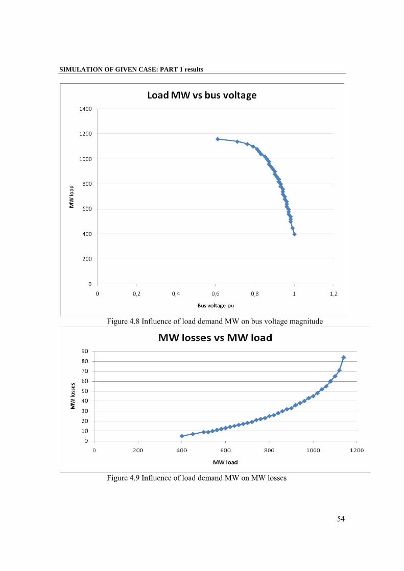
SIMULATION OF GIVEN CASE: PART 1 results
54
Figure 4.8 Influence of load demand MW on bus voltage magnitude
Figure 4.9 Influence of load demand MW on MW losses
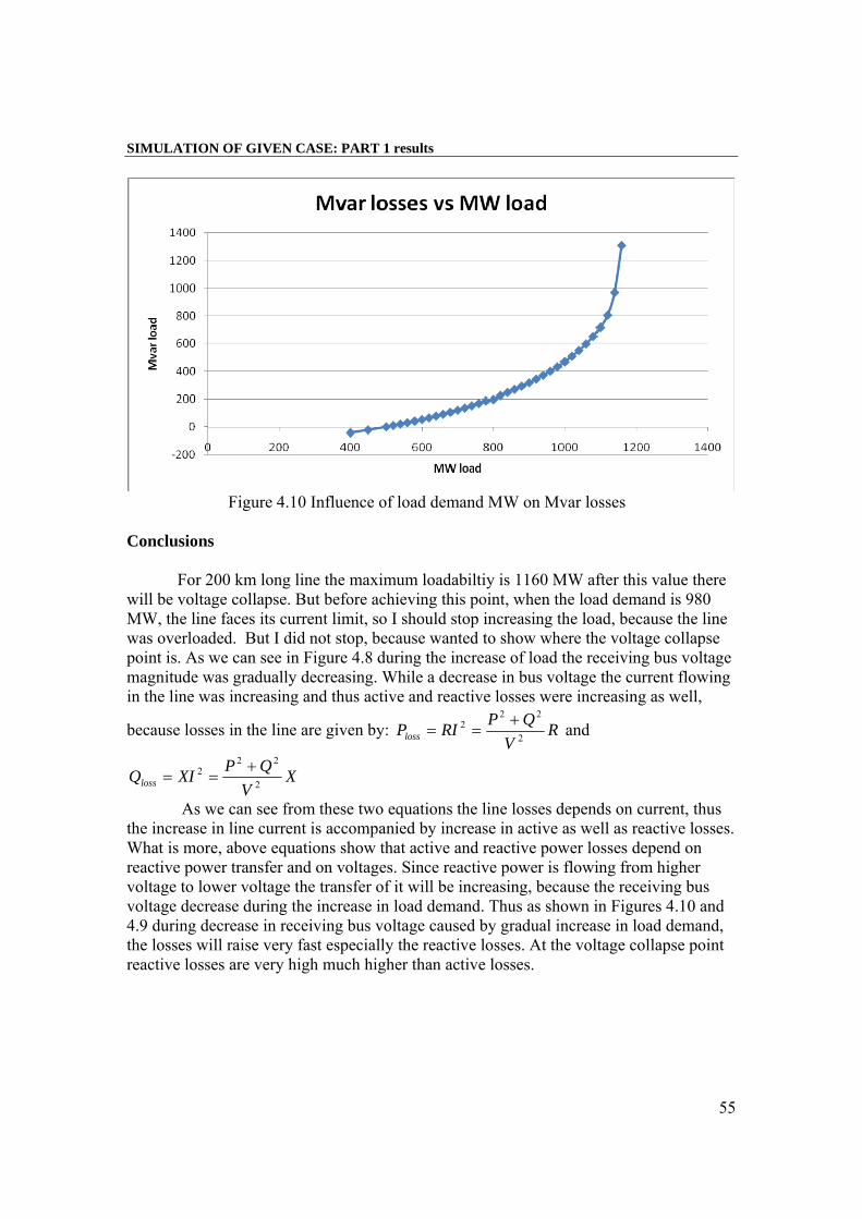
SIMULATION OF GIVEN CASE: PART 1 results
55
Figure 4.10 Influence of load demand MW on Mvar losses Conclusions
For 200 km long line the maximum loadabiltiy is 1160 MW after this value there will be voltage collapse. But before achieving this point, when the load demand is 980 MW, the line faces its current limit, so I should stop increasing the load, because the line was overloaded. But I did not stop, because wanted to show where the voltage collapse point is. As we can see in Figure 4.8 during the increase of load the receiving bus voltage magnitude was gradually decreasing. While a decrease in bus voltage the current flowing in the line was increasing and thus active and reactive losses were increasing as well,
because losses in the line are given by: RV
QPRIPloss 2
222 +
== and
XV
QPXIQloss 2
222 +
==
As we can see from these two equations the line losses depends on current, thus the increase in line current is accompanied by increase in active as well as reactive losses. What is more, above equations show that active and reactive power losses depend on reactive power transfer and on voltages. Since reactive power is flowing from higher voltage to lower voltage the transfer of it will be increasing, because the receiving bus voltage decrease during the increase in load demand. Thus as shown in Figures 4.10 and 4.9 during decrease in receiving bus voltage caused by gradual increase in load demand, the losses will raise very fast especially the reactive losses. At the voltage collapse point reactive losses are very high much higher than active losses.
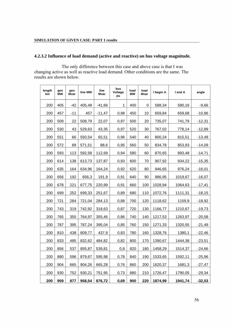
SIMULATION OF GIVEN CASE: PART 1 results
56
4.2.3.2 Influence of load demand (active and reactive) on bus voltage magnitude. The only difference between this case and above case is that I was
changing active as well as reactive load demand. Other conditions are the same. The results are shown below.
length km
gen MW
gen Mvar line MW line
Mvar bus
Voltage pu
load MW
load Mvar I begin A I end A angle
200 405 -42 405,48 -41,66 1 400 0 588,34 580,16 -9,66
200 457 -11 457 -11,47 0,98 450 10 659,84 659,68 -10,96
200 509 22 508,79 22,07 0,97 500 20 735,07 741,79 -12,31
200 530 43 529,63 43,35 0,97 520 30 767,02 778,14 -12,89
200 551 66 550,54 65,51 0,96 540 40 800,24 815,51 -13,48
200 572 89 571,51 88,6 0,95 560 50 834,78 853,93 -14,09
200 593 113 592,58 112,69 0,94 580 60 870,65 893,48 -14,71
200 614 138 613,73 137,87 0,93 600 70 907,92 934,22 -15,35
200 635 164 634,96 164,24 0,92 620 80 946,65 976,24 -16,01
200 656 192 656,3 191,9 0,91 640 90 986,95 1019,67 -16,07
200 678 221 677,75 220,99 0,91 660 100 1028,94 1064,63 -17,41
200 699 252 699,33 251,67 0,89 680 110 1072,76 1111,31 -18,15
200 721 284 721,04 284,13 0,88 700 120 1118,62 1159,9 -18,92
200 743 319 742,92 318,63 0,87 720 130 1166,77 1210,67 -19,73
200 765 355 764,97 355,46 0,86 740 140 1217,53 1263,97 -20,58
200 787 395 787,24 395,04 0,85 760 150 1271,33 1320,55 -21,49
200 810 438 809,77 437,9 0,83 780 160 1328,76 1380,1 -22,46
200 833 485 832,62 484,82 0,82 800 170 1390,67 1444,38 -23,51
200 856 537 855,87 539,81 0,8 820 180 1458,29 1514,37 -24,66
200 880 596 879,67 595,98 0,78 840 190 1533,65 1592,11 -25,96
200 904 665 904,26 665,28 0,76 860 200 1620,37 1681,3 -27,47
200 930 752 930,21 751,95 0,73 880 210 1726,47 1790,05 -29,34
200 959 877 958,54 876,72 0,69 900 220 1874,99 1941,74 -32,03
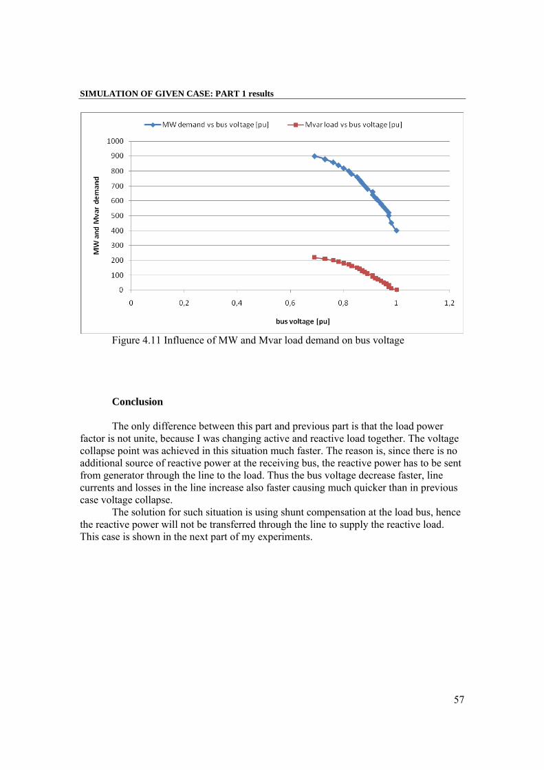
SIMULATION OF GIVEN CASE: PART 1 results
57
Figure 4.11 Influence of MW and Mvar load demand on bus voltage Conclusion The only difference between this part and previous part is that the load power
factor is not unite, because I was changing active and reactive load together. The voltage collapse point was achieved in this situation much faster. The reason is, since there is no additional source of reactive power at the receiving bus, the reactive power has to be sent from generator through the line to the load. Thus the bus voltage decrease faster, line currents and losses in the line increase also faster causing much quicker than in previous case voltage collapse.
The solution for such situation is using shunt compensation at the load bus, hence the reactive power will not be transferred through the line to supply the reactive load. This case is shown in the next part of my experiments.
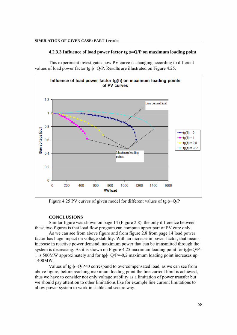
SIMULATION OF GIVEN CASE: PART 1 results
58
4.2.3.3 Influence of load power factor tg φ=Q/P on maximum loading point This experiment investigates how PV curve is changing according to different
values of load power factor tg φ=Q/P. Results are illustrated on Figure 4.25.
Figure 4.25 PV curves of given model for different values of tg φ=Q/P CONCLUSIONS Similar figure was shown on page 14 (Figure 2.8), the only difference between these two figures is that load flow program can compute upper part of PV cure only.
As we can see from above figure and from figure 2.8 from page 14 load power factor has huge impact on voltage stability. With an increase in power factor, that means increase in reactive power demand, maximum power that can be transmitted through the system is decreasing. As it is shown on Figure 4.25 maximum loading point for tgφ=Q/P= 1 is 500MW approximately and for tgφ=Q/P=-0,2 maximum loading point increases up 1400MW.
Values of tg φ=Q/P<0 correspond to overcompensated load, as we can see from above figure, before reaching maximum loading point the line current limit is achieved, thus we have to consider not only voltage stability as a limitation of power transfer but we should pay attention to other limitations like for example line current limitations to allow power system to work in stable and secure way.
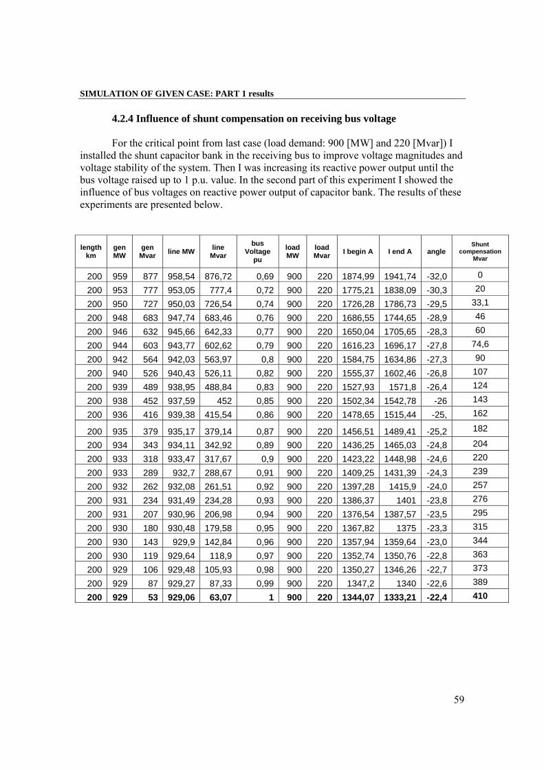
SIMULATION OF GIVEN CASE: PART 1 results
59
4.2.4 Influence of shunt compensation on receiving bus voltage For the critical point from last case (load demand: 900 [MW] and 220 [Mvar]) I
installed the shunt capacitor bank in the receiving bus to improve voltage magnitudes and voltage stability of the system. Then I was increasing its reactive power output until the bus voltage raised up to 1 p.u. value. In the second part of this experiment I showed the influence of bus voltages on reactive power output of capacitor bank. The results of these experiments are presented below.
length km
gen MW
gen Mvar line MW line
Mvar bus
Voltage pu
load MW
load Mvar I begin A I end A angle
Shunt compensation
Mvar
200 959 877 958,54 876,72 0,69 900 220 1874,99 1941,74 -32,0 0
200 953 777 953,05 777,4 0,72 900 220 1775,21 1838,09 -30,3 20
200 950 727 950,03 726,54 0,74 900 220 1726,28 1786,73 -29,5 33,1
200 948 683 947,74 683,46 0,76 900 220 1686,55 1744,65 -28,9 46
200 946 632 945,66 642,33 0,77 900 220 1650,04 1705,65 -28,3 60
200 944 603 943,77 602,62 0,79 900 220 1616,23 1696,17 -27,8 74,6
200 942 564 942,03 563,97 0,8 900 220 1584,75 1634,86 -27,3 90
200 940 526 940,43 526,11 0,82 900 220 1555,37 1602,46 -26,8 107
200 939 489 938,95 488,84 0,83 900 220 1527,93 1571,8 -26,4 124
200 938 452 937,59 452 0,85 900 220 1502,34 1542,78 -26 143
200 936 416 939,38 415,54 0,86 900 220 1478,65 1515,44 -25, 162
200 935 379 935,17 379,14 0,87 900 220 1456,51 1489,41 -25,2 182
200 934 343 934,11 342,92 0,89 900 220 1436,25 1465,03 -24,8 204
200 933 318 933,47 317,67 0,9 900 220 1423,22 1448,98 -24,6 220
200 933 289 932,7 288,67 0,91 900 220 1409,25 1431,39 -24,3 239
200 932 262 932,08 261,51 0,92 900 220 1397,28 1415,9 -24,0 257
200 931 234 931,49 234,28 0,93 900 220 1386,37 1401 -23,8 276
200 931 207 930,96 206,98 0,94 900 220 1376,54 1387,57 -23,5 295
200 930 180 930,48 179,58 0,95 900 220 1367,82 1375 -23,3 315
200 930 143 929,9 142,84 0,96 900 220 1357,94 1359,64 -23,0 344
200 930 119 929,64 118,9 0,97 900 220 1352,74 1350,76 -22,8 363
200 929 106 929,48 105,93 0,98 900 220 1350,27 1346,26 -22,7 373
200 929 87 929,27 87,33 0,99 900 220 1347,2 1340 -22,6 389
200 929 53 929,06 63,07 1 900 220 1344,07 1333,21 -22,4 410
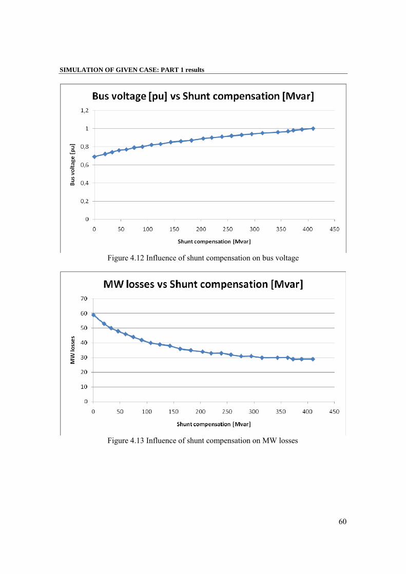
SIMULATION OF GIVEN CASE: PART 1 results
60
Figure 4.12 Influence of shunt compensation on bus voltage
Figure 4.13 Influence of shunt compensation on MW losses
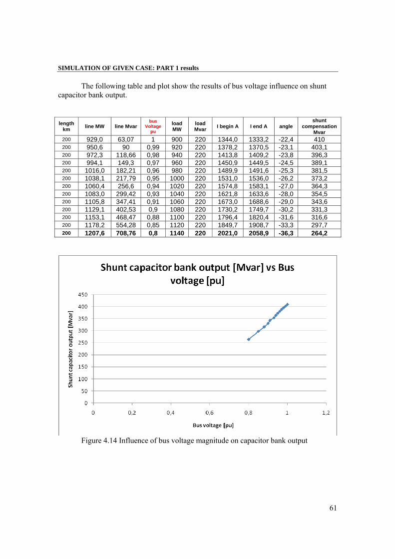
SIMULATION OF GIVEN CASE: PART 1 results
61
The following table and plot show the results of bus voltage influence on shunt capacitor bank output. length
km line MW line Mvar bus
Voltage pu
load MW
load Mvar I begin A I end A angle
shunt compensation
Mvar 200 929,0 63,07 1 900 220 1344,0 1333,2 -22,4 410 200 950,6 90 0,99 920 220 1378,2 1370,5 -23,1 403,1 200 972,3 118,66 0,98 940 220 1413,8 1409,2 -23,8 396,3 200 994,1 149,3 0,97 960 220 1450,9 1449,5 -24,5 389,1 200 1016,0 182,21 0,96 980 220 1489,9 1491,6 -25,3 381,5 200 1038,1 217,79 0,95 1000 220 1531,0 1536,0 -26,2 373,2 200 1060,4 256,6 0,94 1020 220 1574,8 1583,1 -27,0 364,3 200 1083,0 299,42 0,93 1040 220 1621,8 1633,6 -28,0 354,5 200 1105,8 347,41 0,91 1060 220 1673,0 1688,6 -29,0 343,6 200 1129,1 402,53 0,9 1080 220 1730,2 1749,7 -30,2 331,3 200 1153,1 468,47 0,88 1100 220 1796,4 1820,4 -31,6 316,6 200 1178,2 554,28 0,85 1120 220 1849,7 1908,7 -33,3 297,7 200 1207,6 708,76 0,8 1140 220 2021,0 2058,9 -36,3 264,2
Figure 4.14 Influence of bus voltage magnitude on capacitor bank output

SIMULATION OF GIVEN CASE: PART 1 results
62
Conclusions What we can conclude from above experiments is that shunt compensation can really improve bus voltage magnitude and voltage stability, but it has some disadvantages as well. Capacitor banks are rather bus than line connected devices. The purpose of installing them is to give the reactive power injection directly in the load area to improve voltage control and load stabilization. As we can see from Figure 4.12 while the increase of shunt capacitor output the bus voltages were also increasing, thus by keeping voltages high the compensation reduces the line losses, because the line current decreases and since active as well as reactive power losses are given by: P=RI 2 and Q=XI 2 they also decrease. What is more, the shunt compensation increase the bus voltage because, if there is source of reactive power directly connected to load bus, there is no need of transmitting this power through the line. The influence of shunt capacitor bank compensation on line losses is shown in Figure 4.13. Another advantage of shunt compensation is that it improves load power factor (tg φ=Q/P) decreases it. As it is shown on Figure 2.8, page 14 additional load compensation (decrement of the value of tg φ=Q/P) is beneficial for the power system, because it extend its characteristic. Thus the maximum loading point is much higher than without compensation. The opportunity to increase power system loading by shunt compensation is valuable nowadays. Usually the compensation investments are cheaper and more environmental friendly than line investments. However, as was mentioned before shunt compensation has also disadvantages. The main one is the dependence of reactive power output of shunt capacitor bank, on voltages. According to equation Q = BU 2 , the obvious shortcoming of shunt capacitor banks is that the reactive power output drops with the voltage squared. This situation is shown in Figure 4.14. As we can see from this Figure during low voltage profiles shunt capacitor bank does not work properly, and thus they may contribute to faster voltage collapse.
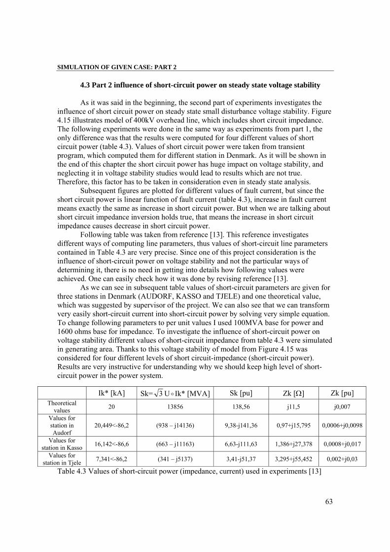
SIMULATION OF GIVEN CASE: PART 2
63
4.3 Part 2 influence of short-circuit power on steady state voltage stability As it was said in the beginning, the second part of experiments investigates the
influence of short circuit power on steady state small disturbance voltage stability. Figure 4.15 illustrates model of 400kV overhead line, which includes short circuit impedance. The following experiments were done in the same way as experiments from part 1, the only difference was that the results were computed for four different values of short circuit power (table 4.3). Values of short circuit power were taken from transient program, which computed them for different station in Denmark. As it will be shown in the end of this chapter the short circuit power has huge impact on voltage stability, and neglecting it in voltage stability studies would lead to results which are not true. Therefore, this factor has to be taken in consideration even in steady state analysis.
Subsequent figures are plotted for different values of fault current, but since the short circuit power is linear function of fault current (table 4.3), increase in fault current means exactly the same as increase in short circuit power. But when we are talking about short circuit impedance inversion holds true, that means the increase in short circuit impedance causes decrease in short circuit power.
Following table was taken from reference [13]. This reference investigates different ways of computing line parameters, thus values of short-circuit line parameters contained in Table 4.3 are very precise. Since one of this project consideration is the influence of short-circuit power on voltage stability and not the particular ways of determining it, there is no need in getting into details how following values were achieved. One can easily check how it was done by revising reference [13].
As we can see in subsequent table values of short-circuit parameters are given for three stations in Denmark (AUDORF, KASSO and TJELE) and one theoretical value, which was suggested by supervisor of the project. We can also see that we can transform very easily short-circuit current into short-circuit power by solving very simple equation. To change following parameters to per unit values I used 100MVA base for power and 1600 ohms base for impedance. To investigate the influence of short-circuit power on voltage stability different values of short-circuit impedance from table 4.3 were simulated in generating area. Thanks to this voltage stability of model from Figure 4.15 was considered for four different levels of short circuit-impedance (short-circuit power). Results are very instructive for understanding why we should keep high level of short-circuit power in the power system.
Table 4.3 Values of short-circuit power (impedance, current) used in experiments [13]
Ik* [kA] Sk= 3 U o Ik* [MVA] Sk [pu] Zk [Ω] Zk [pu] Theoretical
values 20 13856 138,56 j11,5 j0,007
Values for station in Audorf
20,449<-86,2 (938 – j14136) 9,38-j141,36 0,97+j15,795 0,0006+j0,0098
Values for station in Kasso 16,142<-86,6 (663 – j11163) 6,63-j111,63 1,386+j27,378 0,0008+j0,017
Values for station in Tjele 7,341<-86,2 (341 – j5137) 3,41-j51,37 3,295+j55,452 0,002+j0,03
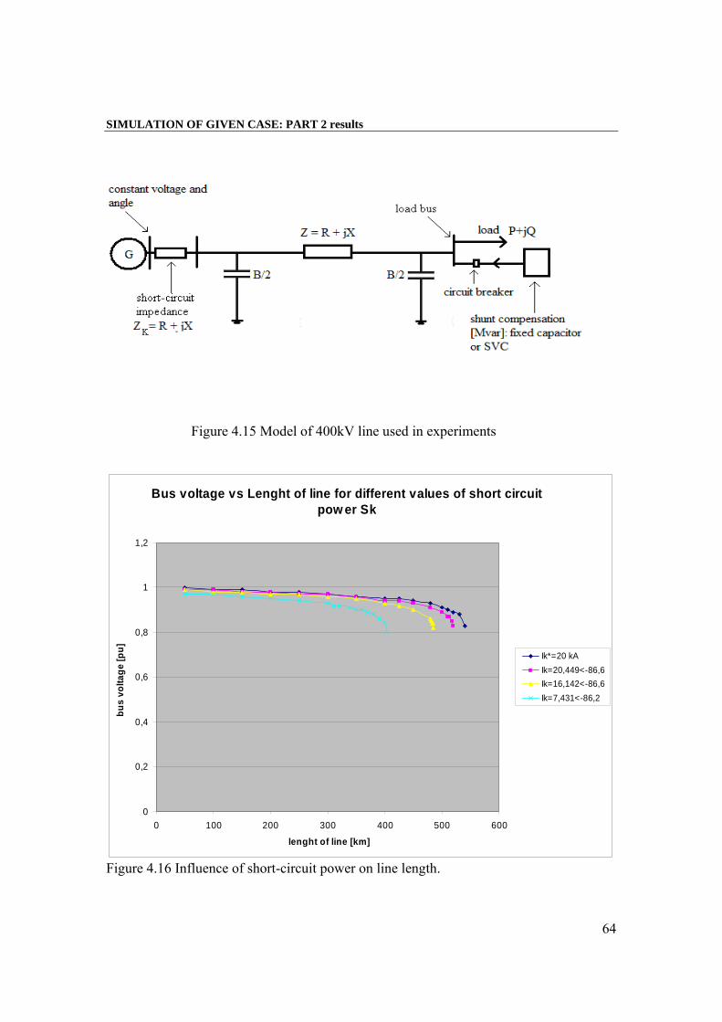
SIMULATION OF GIVEN CASE: PART 2 results
64
Figure 4.15 Model of 400kV line used in experiments
Bus voltage vs Lenght of line for different values of short circuit pow er Sk
0
0,2
0,4
0,6
0,8
1
1,2
0 100 200 300 400 500 600
lenght of line [km]
bus
volta
ge [p
u]
Ik*=20 kAIk=20,449<-86,6Ik=16,142<-86,6Ik=7,431<-86,2
Figure 4.16 Influence of short-circuit power on line length.
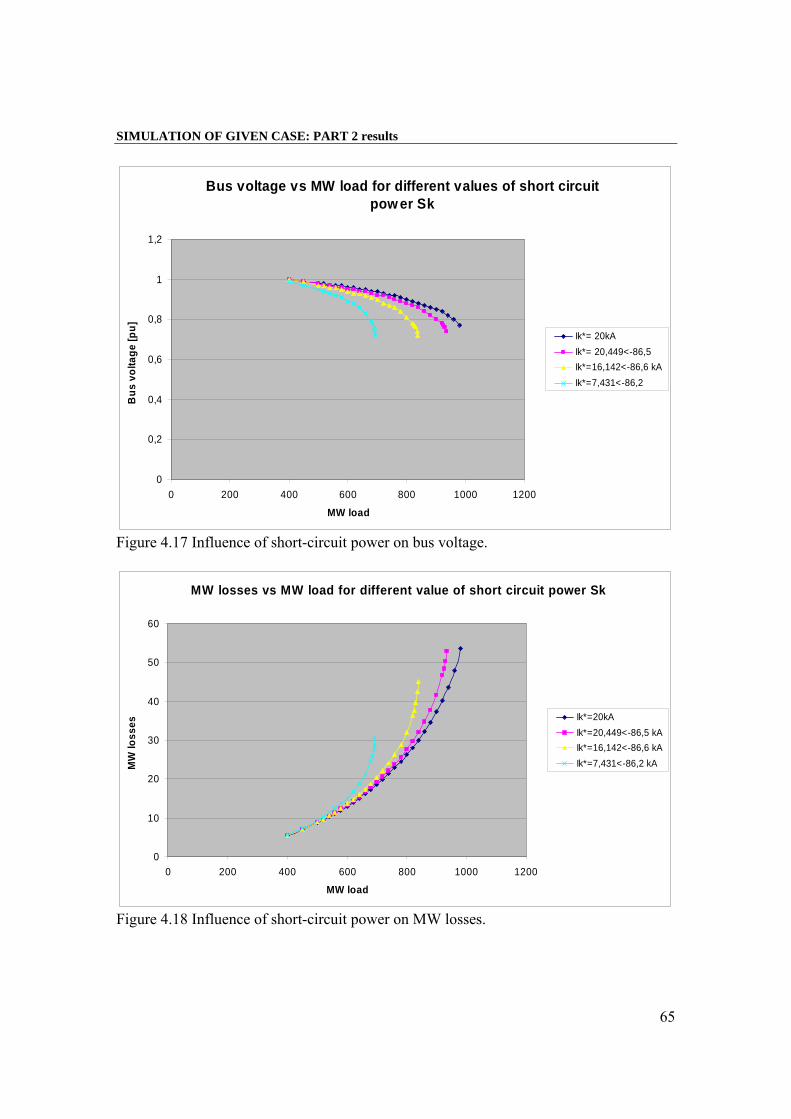
SIMULATION OF GIVEN CASE: PART 2 results
65
Bus voltage vs MW load for different values of short circuit pow er Sk
0
0,2
0,4
0,6
0,8
1
1,2
0 200 400 600 800 1000 1200
MW load
Bus
vol
tage
[pu]
Ik*= 20kAIk*= 20,449<-86,5Ik*=16,142<-86,6 kAIk*=7,431<-86,2
Figure 4.17 Influence of short-circuit power on bus voltage.
MW losses vs MW load for different value of short circuit power Sk
0
10
20
30
40
50
60
0 200 400 600 800 1000 1200
MW load
MW
loss
es
Ik*=20kAIk*=20,449<-86,5 kAIk*=16,142<-86,6 kAIk*=7,431<-86,2 kA
Figure 4.18 Influence of short-circuit power on MW losses.
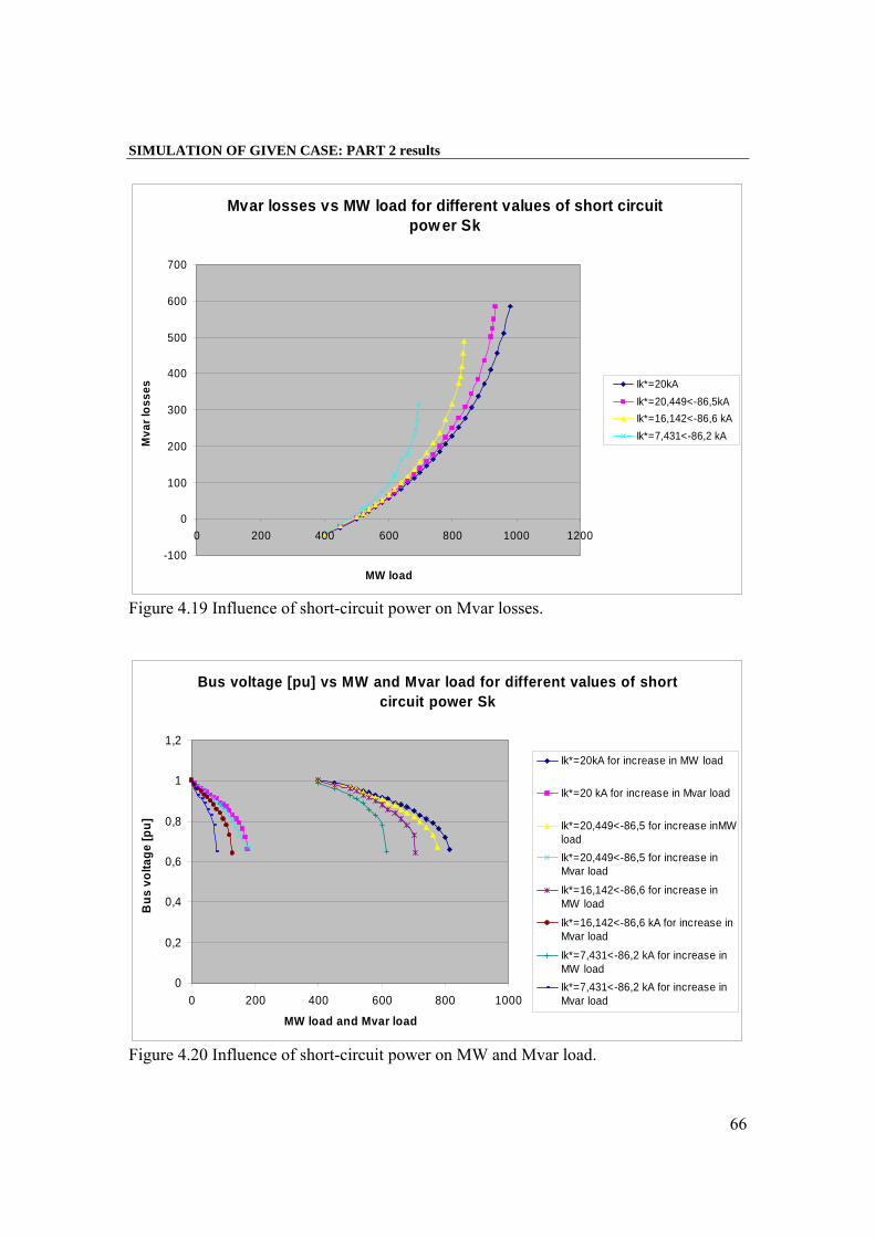
SIMULATION OF GIVEN CASE: PART 2 results
66
Mvar losses vs MW load for different values of short circuit pow er Sk
-100
0
100
200
300
400
500
600
700
0 200 400 600 800 1000 1200
MW load
Mva
r los
ses Ik*=20kA
Ik*=20,449<-86,5kAIk*=16,142<-86,6 kAIk*=7,431<-86,2 kA
Figure 4.19 Influence of short-circuit power on Mvar losses.
Bus voltage [pu] vs MW and Mvar load for different values of short circuit power Sk
0
0,2
0,4
0,6
0,8
1
1,2
0 200 400 600 800 1000
MW load and Mvar load
Bus
vol
tage
[pu]
Ik*=20kA for increase in MW load
Ik*=20 kA for increase in Mvar load
Ik*=20,449<-86,5 for increase inMWloadIk*=20,449<-86,5 for increase inMvar load
Ik*=16,142<-86,6 for increase inMW load
Ik*=16,142<-86,6 kA for increase inMvar load
Ik*=7,431<-86,2 kA for increase inMW loadIk*=7,431<-86,2 kA for increase inMvar load
Figure 4.20 Influence of short-circuit power on MW and Mvar load.
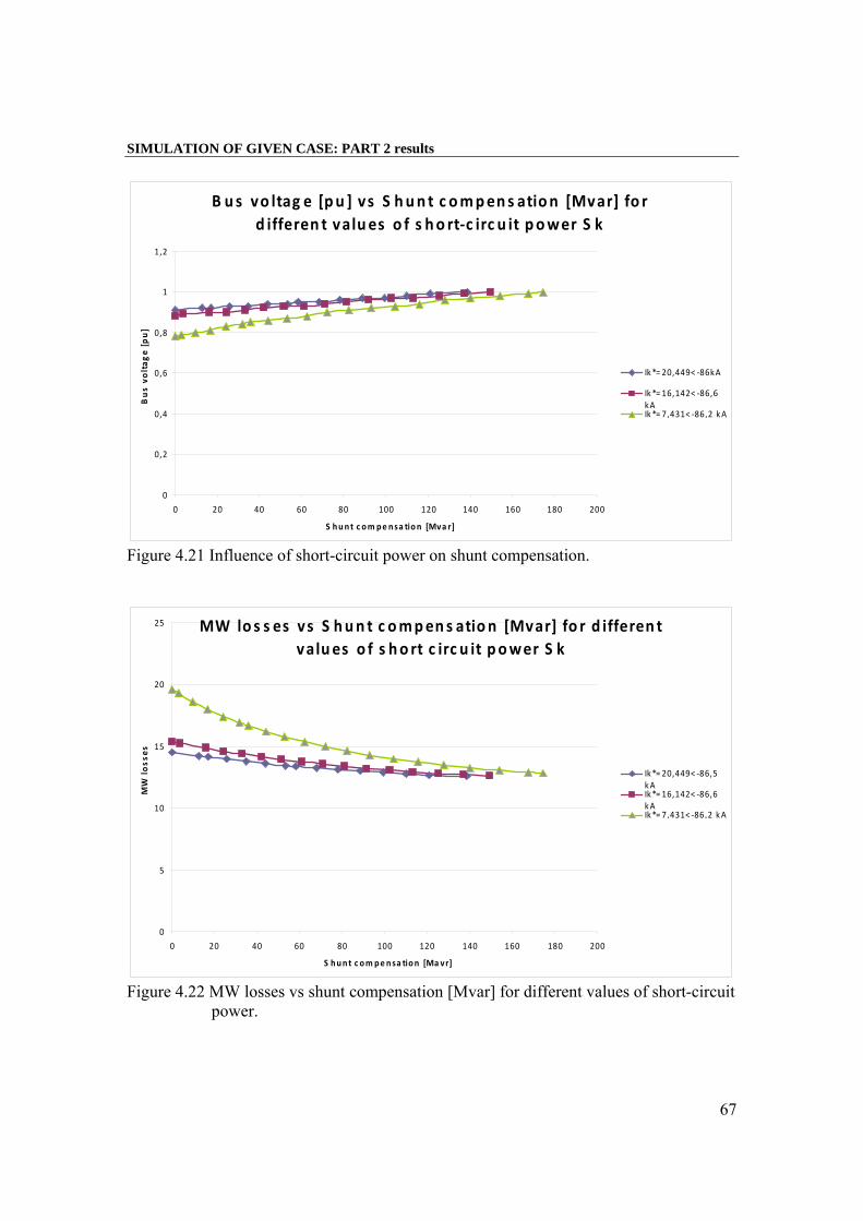
SIMULATION OF GIVEN CASE: PART 2 results
67
B us vo ltag e [pu ] vs S hun t c ompens ation [Mvar] fo r d ifferen t values o f s ho rt‐c irc u it power S k
0
0,2
0,4
0,6
0,8
1
1,2
0 20 40 60 80 100 120 140 160 180 200
S hunt c om pe nsa tion [Mva r]
Bus vo
ltag
e [pu]
Ik*= 20,449< ‐86kA
Ik*= 16,142< ‐86,6kAIk*= 7,431< ‐86,2 kA
Figure 4.21 Influence of short-circuit power on shunt compensation.
MW lo s s es vs S hun t c ompens ation [Mvar] fo r d ifferen t values o f s ho rt c irc u it power S k
0
5
10
15
20
25
0 20 40 60 80 100 120 140 160 180 200
S hunt c om pensa tion [Ma vr]
MW
loss
es
Ik*= 20,449< ‐86,5kAIk*= 16,142< ‐86,6kAIk*= 7,431< ‐86,2 kA
Figure 4.22 MW losses vs shunt compensation [Mvar] for different values of short-circuit power.
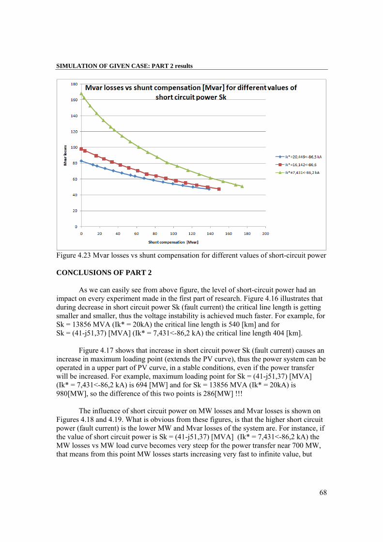
SIMULATION OF GIVEN CASE: PART 2 results
68
Figure 4.23 Mvar losses vs shunt compensation for different values of short-circuit power CONCLUSIONS OF PART 2 As we can easily see from above figure, the level of short-circuit power had an impact on every experiment made in the first part of research. Figure 4.16 illustrates that during decrease in short circuit power Sk (fault current) the critical line length is getting smaller and smaller, thus the voltage instability is achieved much faster. For example, for Sk = 13856 MVA (Ik* = 20kA) the critical line length is 540 [km] and for Sk = (41-j51,37) [MVA] (Ik* = 7,431<-86,2 kA) the critical line length 404 [km]. Figure 4.17 shows that increase in short circuit power Sk (fault current) causes an increase in maximum loading point (extends the PV curve), thus the power system can be operated in a upper part of PV curve, in a stable conditions, even if the power transfer will be increased. For example, maximum loading point for Sk = (41-j51,37) [MVA] (Ik* = 7,431<-86,2 kA) is 694 [MW] and for Sk = 13856 MVA (Ik* = 20kA) is 980[MW], so the difference of this two points is 286[MW] !!! The influence of short circuit power on MW losses and Mvar losses is shown on Figures 4.18 and 4.19. What is obvious from these figures, is that the higher short circuit power (fault current) is the lower MW and Mvar losses of the system are. For instance, if the value of short circuit power is Sk = (41-j51,37) [MVA] (Ik* = 7,431<-86,2 kA) the MW losses vs MW load curve becomes very steep for the power transfer near 700 MW, that means from this point MW losses starts increasing very fast to infinite value, but
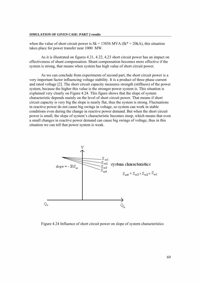
SIMULATION OF GIVEN CASE: PART 2 results
69
when the value of short circuit power is Sk = 13856 MVA (Ik* = 20kA), this situation takes place for power transfer near 1000 MW. As it is illustrated on figures 4.21, 4.22, 4,23 short circuit power has an impact on effectiveness of shunt compensation. Shunt compensation becomes more effective if the system is strong, that means when system has high value of short circuit power. As we can conclude from experiments of second part, the short circuit power is a very important factor influencing voltage stability. It is a product of three phase current and rated voltage [2]. The short circuit capacity measures strength (stiffness) of the power system, because the higher this value is the stronger power system is. This situation is explained very clearly on Figure 4.24. This figure shows that the slope of system characteristic depends mainly on the level of short circuit power. That means if short circuit capacity is very big the slope is nearly flat, thus the system is strong. Fluctuations in reactive power do not cause big swings in voltage, so system can work in stable conditions even during the change in reactive power demand. But when the short circuit power is small, the slope of system’s characteristic becomes steep, which means that even a small changes in reactive power demand can cause big swings of voltage, thus in this situation we can tell that power system is weak.
Figure 4.24 Influence of short circuit power on slope of system characteristics

SIMULATION OF GIVEN CASE: PART 2 results
70
We have to keep in mind that the power plants are main source of short circuit power. If for example some contingency will lead to tripping off the power plant, the short circuit power of particular power system will decrease rapidly. Moreover, the sudden decrease in short circuit power makes system weak, thus even small changes in reactive power cause voltage swings, and when voltages started to decrease the need for reactive power increases even more which can lead to voltage instability and further to voltage collapse. From stability point of view we should keep the fault current (short circuit capacity) level as highest as possible, but from economical point of view it is not so obvious. Because the high fault current means that we have to use bigger circuit-barkers, bigger circuit-barkers mean more expensive circuit-breakers. Thus the decision about short-circuit level should be a compromise between these two points of view, because stability reasons as well as economical reasons are very important for making particular decision.
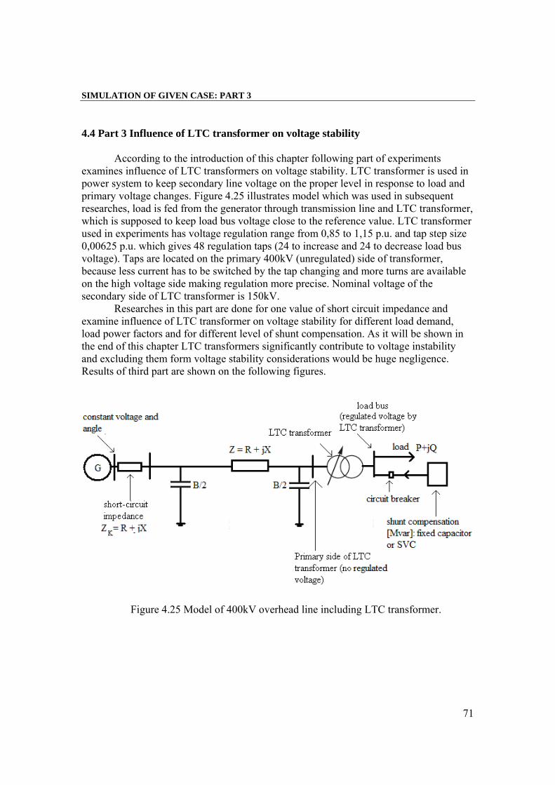
SIMULATION OF GIVEN CASE: PART 3
71
4.4 Part 3 Influence of LTC transformer on voltage stability According to the introduction of this chapter following part of experiments examines influence of LTC transformers on voltage stability. LTC transformer is used in power system to keep secondary line voltage on the proper level in response to load and primary voltage changes. Figure 4.25 illustrates model which was used in subsequent researches, load is fed from the generator through transmission line and LTC transformer, which is supposed to keep load bus voltage close to the reference value. LTC transformer used in experiments has voltage regulation range from 0,85 to 1,15 p.u. and tap step size 0,00625 p.u. which gives 48 regulation taps (24 to increase and 24 to decrease load bus voltage). Taps are located on the primary 400kV (unregulated) side of transformer, because less current has to be switched by the tap changing and more turns are available on the high voltage side making regulation more precise. Nominal voltage of the secondary side of LTC transformer is 150kV. Researches in this part are done for one value of short circuit impedance and examine influence of LTC transformer on voltage stability for different load demand, load power factors and for different level of shunt compensation. As it will be shown in the end of this chapter LTC transformers significantly contribute to voltage instability and excluding them form voltage stability considerations would be huge negligence. Results of third part are shown on the following figures.
Figure 4.25 Model of 400kV overhead line including LTC transformer.
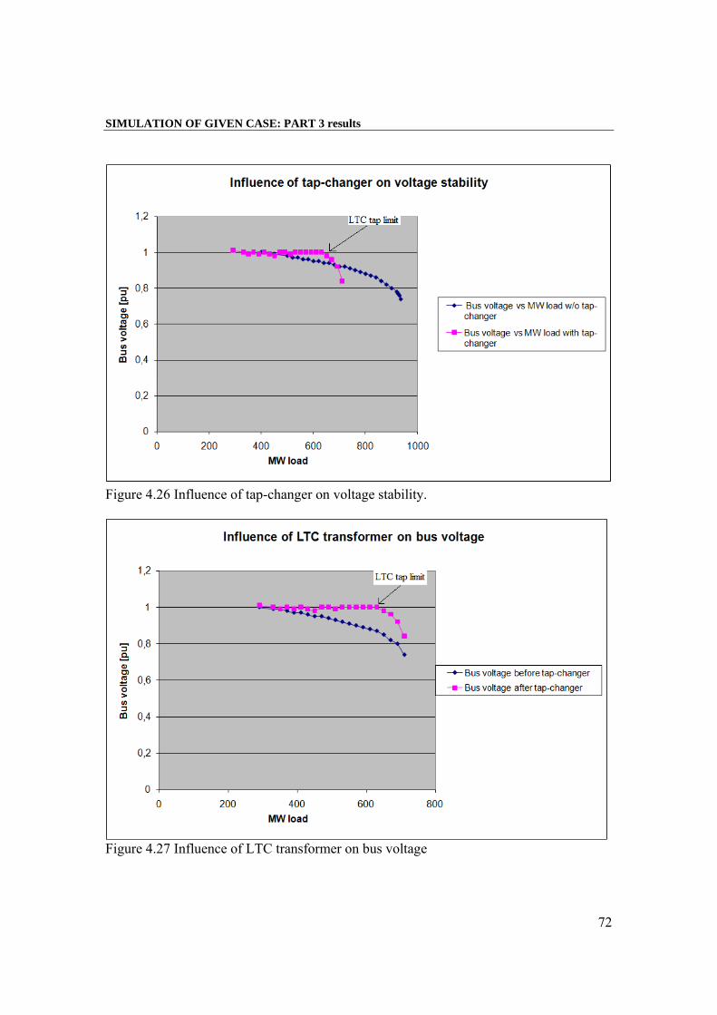
SIMULATION OF GIVEN CASE: PART 3 results
72
Figure 4.26 Influence of tap-changer on voltage stability.
Figure 4.27 Influence of LTC transformer on bus voltage
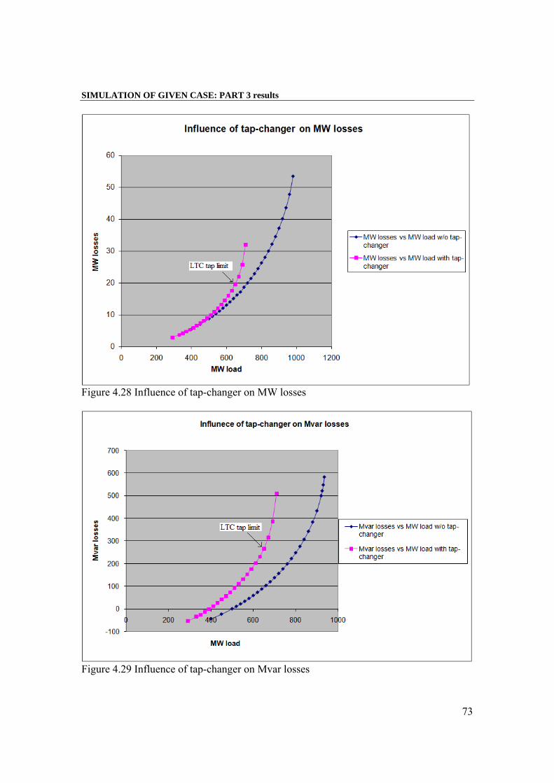
SIMULATION OF GIVEN CASE: PART 3 results
73
Figure 4.28 Influence of tap-changer on MW losses
Figure 4.29 Influence of tap-changer on Mvar losses

SIMULATION OF GIVEN CASE: PART 3 results
74
Figure 4.30 Influence of load power factor and tap-changer on maximum loading point.
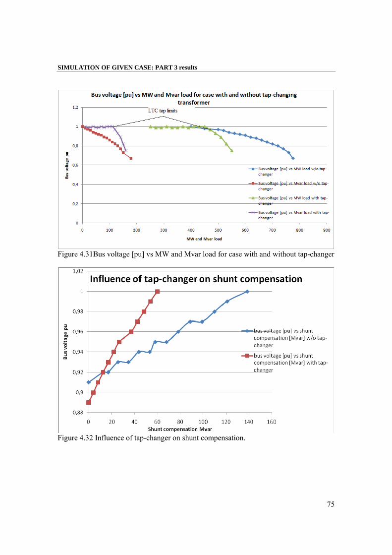
SIMULATION OF GIVEN CASE: PART 3 results
75
Figure 4.31Bus voltage [pu] vs MW and Mvar load for case with and without tap-changer
Figure 4.32 Influence of tap-changer on shunt compensation.
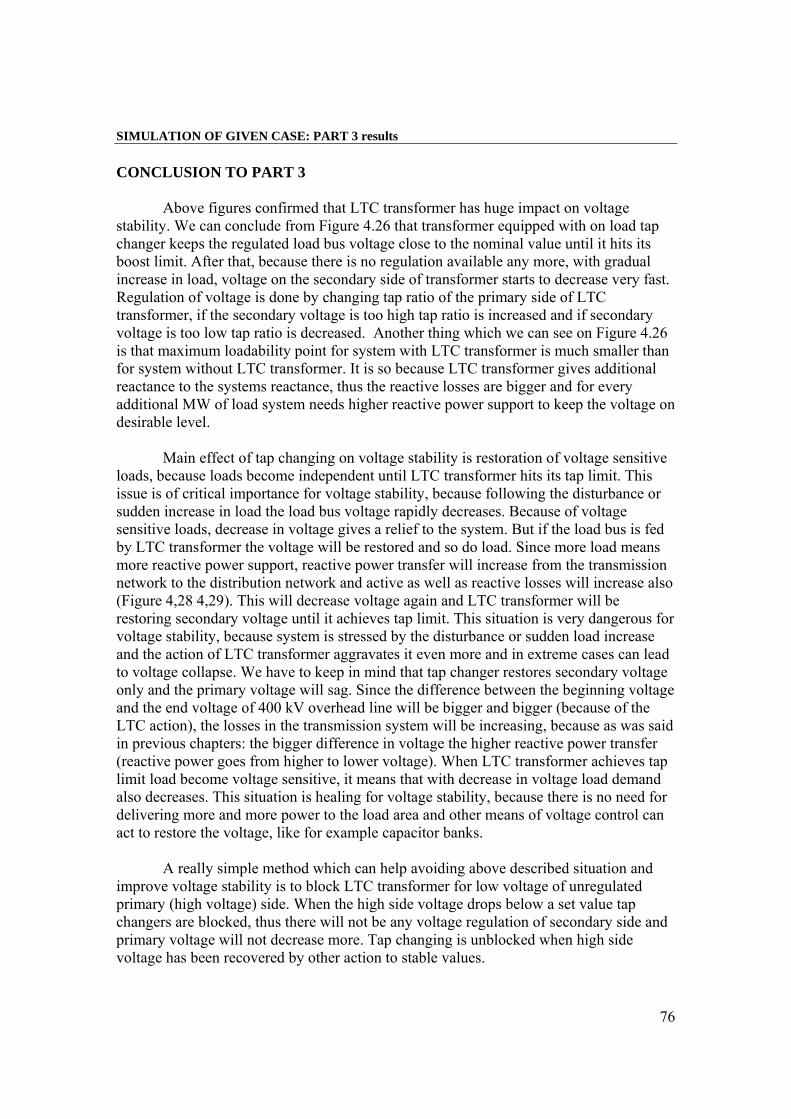
SIMULATION OF GIVEN CASE: PART 3 results
76
CONCLUSION TO PART 3 Above figures confirmed that LTC transformer has huge impact on voltage stability. We can conclude from Figure 4.26 that transformer equipped with on load tap changer keeps the regulated load bus voltage close to the nominal value until it hits its boost limit. After that, because there is no regulation available any more, with gradual increase in load, voltage on the secondary side of transformer starts to decrease very fast. Regulation of voltage is done by changing tap ratio of the primary side of LTC transformer, if the secondary voltage is too high tap ratio is increased and if secondary voltage is too low tap ratio is decreased. Another thing which we can see on Figure 4.26 is that maximum loadability point for system with LTC transformer is much smaller than for system without LTC transformer. It is so because LTC transformer gives additional reactance to the systems reactance, thus the reactive losses are bigger and for every additional MW of load system needs higher reactive power support to keep the voltage on desirable level.
Main effect of tap changing on voltage stability is restoration of voltage sensitive loads, because loads become independent until LTC transformer hits its tap limit. This issue is of critical importance for voltage stability, because following the disturbance or sudden increase in load the load bus voltage rapidly decreases. Because of voltage sensitive loads, decrease in voltage gives a relief to the system. But if the load bus is fed by LTC transformer the voltage will be restored and so do load. Since more load means more reactive power support, reactive power transfer will increase from the transmission network to the distribution network and active as well as reactive losses will increase also (Figure 4,28 4,29). This will decrease voltage again and LTC transformer will be restoring secondary voltage until it achieves tap limit. This situation is very dangerous for voltage stability, because system is stressed by the disturbance or sudden load increase and the action of LTC transformer aggravates it even more and in extreme cases can lead to voltage collapse. We have to keep in mind that tap changer restores secondary voltage only and the primary voltage will sag. Since the difference between the beginning voltage and the end voltage of 400 kV overhead line will be bigger and bigger (because of the LTC action), the losses in the transmission system will be increasing, because as was said in previous chapters: the bigger difference in voltage the higher reactive power transfer (reactive power goes from higher to lower voltage). When LTC transformer achieves tap limit load become voltage sensitive, it means that with decrease in voltage load demand also decreases. This situation is healing for voltage stability, because there is no need for delivering more and more power to the load area and other means of voltage control can act to restore the voltage, like for example capacitor banks.
A really simple method which can help avoiding above described situation and
improve voltage stability is to block LTC transformer for low voltage of unregulated primary (high voltage) side. When the high side voltage drops below a set value tap changers are blocked, thus there will not be any voltage regulation of secondary side and primary voltage will not decrease more. Tap changing is unblocked when high side voltage has been recovered by other action to stable values.
SIMULATION OF GIVEN CASE: PART 3 results
77
Figure 4.32 illustrates very important principle, which says that voltage regulation
by tap changing can improve voltage stability. This is true for the loads which are heavy compensated. The explanation is very simple, since the shunt capacitor compensation has a voltage squared reactive power sensitivity the main effect of tap changing is supporting the capacitor bank output [2]. According to this principle whenever is possible we should place capacitor banks on the regulated side of tap changers, because capacitor bank becomes constant reactive power source.
As we can see from above consideration LTC transformers play really important
role in power system voltage stability. They are commonly used throughout almost all levels of voltages in power system, thus we have to take into account the influence of these devices while examining voltage stability phenomena. Neglecting it might lead to too optimistic results, because as it is illustrated on Figure 4.30 the maximum loading point, which is shown on PV curves, is much smaller than in case without LTC transformer. Another very important thing is that with tap changers regulating the load bus voltage, bus voltage magnitude is very bad indicator of proximity to voltage instability, because as we can see on Figures 4.26, 4.27, 430 and 4.31 LTC keeps almost constant secondary voltage (close to the reference value, usually 1 pu) until it hits tap limit, then bus voltage decreases very fast and the maximum loading point is achieved very fast also.
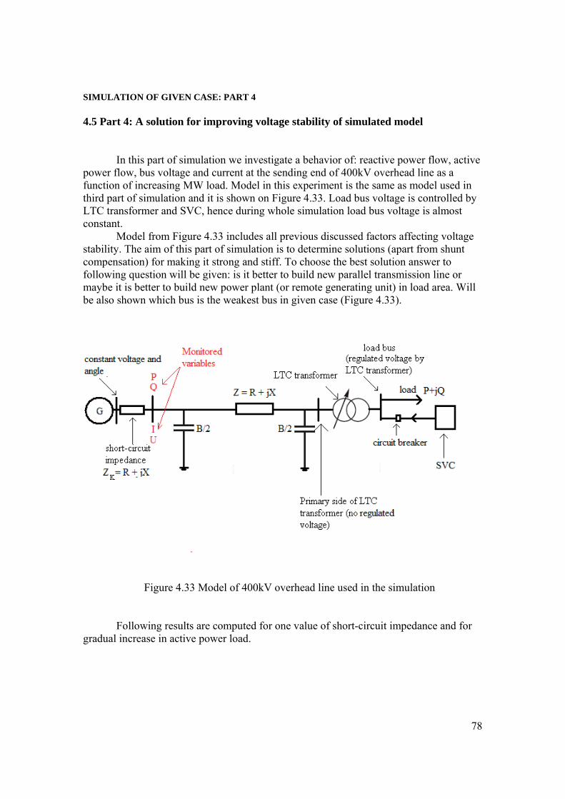
SIMULATION OF GIVEN CASE: PART 4
78
4.5 Part 4: A solution for improving voltage stability of simulated model In this part of simulation we investigate a behavior of: reactive power flow, active power flow, bus voltage and current at the sending end of 400kV overhead line as a function of increasing MW load. Model in this experiment is the same as model used in third part of simulation and it is shown on Figure 4.33. Load bus voltage is controlled by LTC transformer and SVC, hence during whole simulation load bus voltage is almost constant. Model from Figure 4.33 includes all previous discussed factors affecting voltage stability. The aim of this part of simulation is to determine solutions (apart from shunt compensation) for making it strong and stiff. To choose the best solution answer to following question will be given: is it better to build new parallel transmission line or maybe it is better to build new power plant (or remote generating unit) in load area. Will be also shown which bus is the weakest bus in given case (Figure 4.33).
Figure 4.33 Model of 400kV overhead line used in the simulation Following results are computed for one value of short-circuit impedance and for gradual increase in active power load.
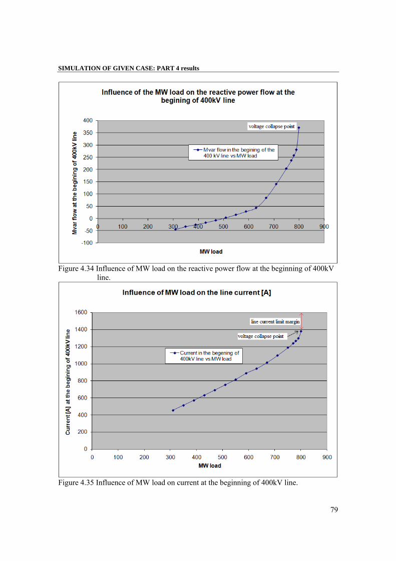
SIMULATION OF GIVEN CASE: PART 4 results
79
Figure 4.34 Influence of MW load on the reactive power flow at the beginning of 400kV line.
Figure 4.35 Influence of MW load on current at the beginning of 400kV line.
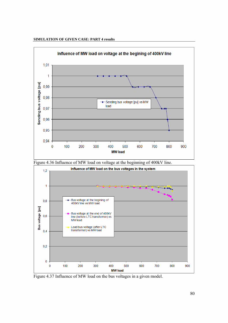
SIMULATION OF GIVEN CASE: PART 4 results
80
Figure 4.36 Influence of MW load on voltage at the beginning of 400kV line.
Figure 4.37 Influence of MW load on the bus voltages in a given model.
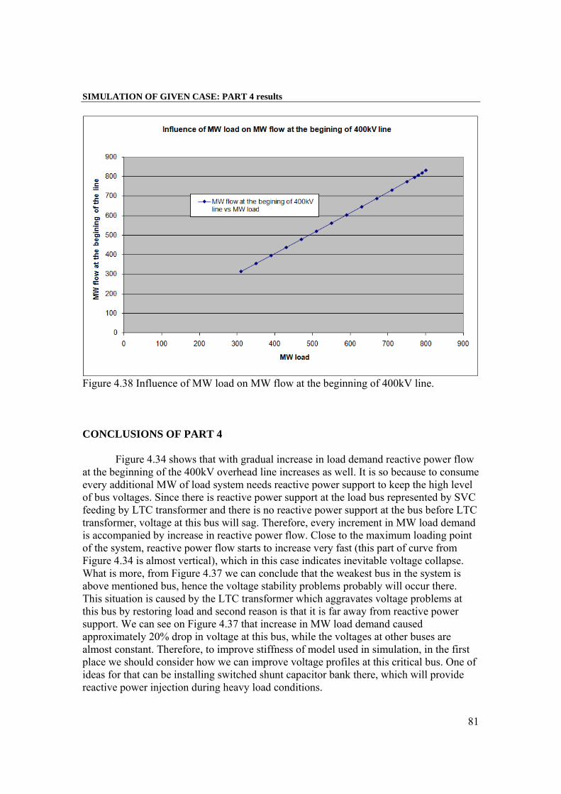
SIMULATION OF GIVEN CASE: PART 4 results
81
Figure 4.38 Influence of MW load on MW flow at the beginning of 400kV line. CONCLUSIONS OF PART 4 Figure 4.34 shows that with gradual increase in load demand reactive power flow at the beginning of the 400kV overhead line increases as well. It is so because to consume every additional MW of load system needs reactive power support to keep the high level of bus voltages. Since there is reactive power support at the load bus represented by SVC feeding by LTC transformer and there is no reactive power support at the bus before LTC transformer, voltage at this bus will sag. Therefore, every increment in MW load demand is accompanied by increase in reactive power flow. Close to the maximum loading point of the system, reactive power flow starts to increase very fast (this part of curve from Figure 4.34 is almost vertical), which in this case indicates inevitable voltage collapse. What is more, from Figure 4.37 we can conclude that the weakest bus in the system is above mentioned bus, hence the voltage stability problems probably will occur there. This situation is caused by the LTC transformer which aggravates voltage problems at this bus by restoring load and second reason is that it is far away from reactive power support. We can see on Figure 4.37 that increase in MW load demand caused approximately 20% drop in voltage at this bus, while the voltages at other buses are almost constant. Therefore, to improve stiffness of model used in simulation, in the first place we should consider how we can improve voltage profiles at this critical bus. One of ideas for that can be installing switched shunt capacitor bank there, which will provide reactive power injection during heavy load conditions.
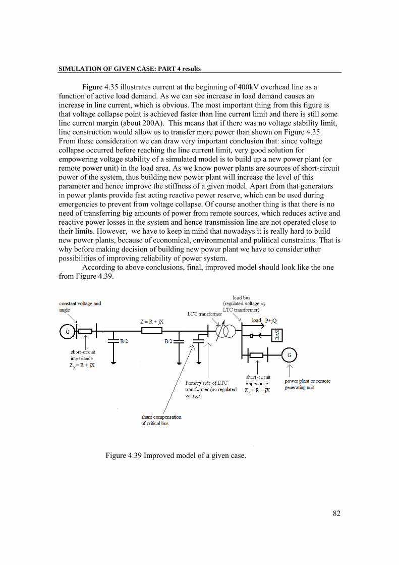
SIMULATION OF GIVEN CASE: PART 4 results
82
Figure 4.35 illustrates current at the beginning of 400kV overhead line as a function of active load demand. As we can see increase in load demand causes an increase in line current, which is obvious. The most important thing from this figure is that voltage collapse point is achieved faster than line current limit and there is still some line current margin (about 200A). This means that if there was no voltage stability limit, line construction would allow us to transfer more power than shown on Figure 4.35. From these consideration we can draw very important conclusion that: since voltage collapse occurred before reaching the line current limit, very good solution for empowering voltage stability of a simulated model is to build up a new power plant (or remote power unit) in the load area. As we know power plants are sources of short-circuit power of the system, thus building new power plant will increase the level of this parameter and hence improve the stiffness of a given model. Apart from that generators in power plants provide fast acting reactive power reserve, which can be used during emergencies to prevent from voltage collapse. Of course another thing is that there is no need of transferring big amounts of power from remote sources, which reduces active and reactive power losses in the system and hence transmission line are not operated close to their limits. However, we have to keep in mind that nowadays it is really hard to build new power plants, because of economical, environmental and political constraints. That is why before making decision of building new power plant we have to consider other possibilities of improving reliability of power system. According to above conclusions, final, improved model should look like the one from Figure 4.39.
Figure 4.39 Improved model of a given case.
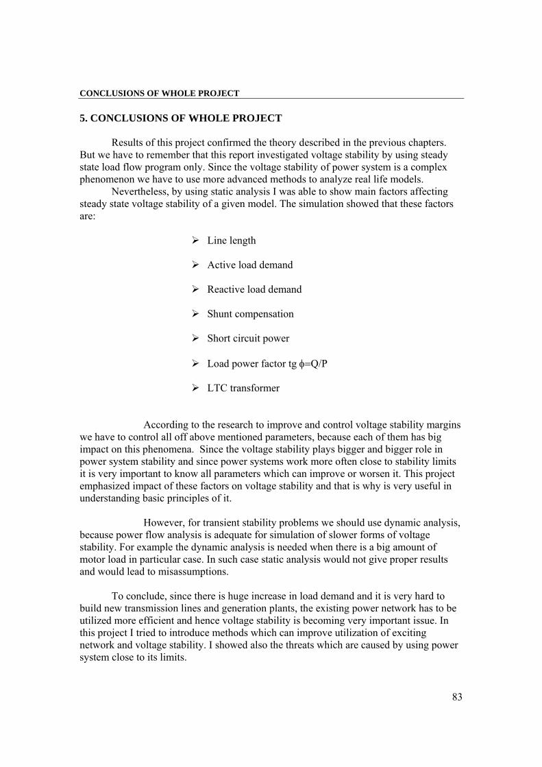
CONCLUSIONS OF WHOLE PROJECT
83
5. CONCLUSIONS OF WHOLE PROJECT
Results of this project confirmed the theory described in the previous chapters. But we have to remember that this report investigated voltage stability by using steady state load flow program only. Since the voltage stability of power system is a complex phenomenon we have to use more advanced methods to analyze real life models.
Nevertheless, by using static analysis I was able to show main factors affecting steady state voltage stability of a given model. The simulation showed that these factors are:
Line length
Active load demand
Reactive load demand
Shunt compensation
Short circuit power
Load power factor tg φ=Q/P
LTC transformer
According to the research to improve and control voltage stability margins
we have to control all off above mentioned parameters, because each of them has big impact on this phenomena. Since the voltage stability plays bigger and bigger role in power system stability and since power systems work more often close to stability limits it is very important to know all parameters which can improve or worsen it. This project emphasized impact of these factors on voltage stability and that is why is very useful in understanding basic principles of it.
However, for transient stability problems we should use dynamic analysis,
because power flow analysis is adequate for simulation of slower forms of voltage stability. For example the dynamic analysis is needed when there is a big amount of motor load in particular case. In such case static analysis would not give proper results and would lead to misassumptions.
To conclude, since there is huge increase in load demand and it is very hard to
build new transmission lines and generation plants, the existing power network has to be utilized more efficient and hence voltage stability is becoming very important issue. In this project I tried to introduce methods which can improve utilization of exciting network and voltage stability. I showed also the threats which are caused by using power system close to its limits.

REFERENCES
84
REFERENCES [1] “Power system stability and control” Prabha Kundur ISBN 0-07-035958-X [2] “Power system voltage stability” Carson W. Taylor ISBN 10-0071137084 [3] “Voltage stability of electric power systems” Thierry Van Cutsen, Costas Vournas ISBN 0-7923-8139-4 [4] “Understanding FACTS” Narain G. Hingorani, Laszlo Gyugyi ISBN 0-7803- 3455-8 [5] H. L. Thanavala D. J. Young and M. H. Baker publication about FACTS Controllers, published by The Institution of Electrical Engineers, London 1999 ISBN 0-85296-771-3 [6] “On-line Voltage Stability Assessment of Power System- An Approach of Black-box Modelling” Sami Repo PhD Thesis
[7] „ Power system analysis” Hadi Saadat ISBN 0-07-116758-7 [8] Lof P-A “On static analysis of long term voltage stability” PhD Thesis, Royal Institute of Technology, Sweden [9] Hirvonen R. and Pottonen L. Low voltages after a disturbance in the Finish 400 kV network [10] Taylor C. W. and Erikson D.C. Recording and analyzing the July 2 Cascading outage, IEEE Computer applications in power, January 1997 [11] “Electrical power distribution and transmission” L. M. Faulkenberry, Walter Coffer ISBN 0-13-249947-9 [12] “Transmission and distribution of electrical energy” Walter L. Weeks ISBN 0-06-046982 [13] “Bestmmelse af ledningskonstanter til netberegniger” ELASAM, Notat N90/NP-201a BCG/BT. 26 August 1991
[14] “Use of series FACTS devices in modern transmission system” Rafał Bukowski MSc. Thesis, Warsaw University of Technology, Poland 1999

REFERENCES
85