HAL Id: hal-02536995https://hal.archives-ouvertes.fr/hal-02536995

Submitted on 8 Apr 2020

HAL is a multi-disciplinary open accessarchive for the deposit and dissemination of sci-entific research documents, whether they are pub-lished or not. The documents may come fromteaching and research institutions in France orabroad, or from public or private research centers.

L’archive ouverte pluridisciplinaire HAL, estdestinée au dépôt et à la diffusion de documentsscientifiques de niveau recherche, publiés ou non,émanant des établissements d’enseignement et derecherche français ou étrangers, des laboratoirespublics ou privés.

Control strategy for the combustion optimization forwaste-to-energy incineration plant

Franco Falconi, Hervé Guillard, Stefan Capitaneanu, Tarek Raissi

To cite this version:Franco Falconi, Hervé Guillard, Stefan Capitaneanu, Tarek Raissi. Control strategy for the combustionoptimization for waste-to-energy incineration plant. 21st IFAC World Congress, Jul 2020, Berlin,Germany. �hal-02536995�

Control strategy for the combustionoptimization for waste-to-energy

incineration plant ?

Franco Falconi ∗ ∗∗ Herve Guillard ∗ Stefan Capitaneanu ∗∗

Tarek Raıssi ∗

∗ Conservatoire National des Arts et Metiers, Paris, France (e-mail:franco.falconi@se.com, herve.guillard@lecnam.net,

tarek.raissi@cnam.fr).∗∗ Schneider Electric, Rueil-Malmaison, France (e-mail:

franco.falconi@se.com, stefan.capitaneanu@se.com)

Abstract: Waste disposal is becoming more and more challenging. Indeed, global population isstill increasing and countries that do not have enough space to create big landfills need to findother solutions to deal with this problem. The incineration of municipal solid waste (MSW), ifwell controlled, is a possible solution. According to Cheng and Hu (2010) incineration can reducethe volume occupied by MSW up to 90% while producing thermal and/or electrical energy. Alsothe bottom ash of incineration can be used in road building and the construction industry. Butair pollution control remains a major problem in the implementation of incineration for solidwaste disposal. Despite the long history of work in this area, the proposed control schemesof these waste-to-energy plants are quite basic. This paper presents a way to optimize such aplant by using Advanced Control techniques. The aim of this operation is to control the steamflow rate, and, therefore the energy production, while ensuring a complete combustion, whichis synonym of minimal pollution emission.

Keywords: Power and Energy Systems, Automation, Modelling, Linear Control, RobustControl, Optimal Control.

1. INTRODUCTION

Waste incineration is a very complex process, mainly be-cause of the high variability of the fuel composition and theinterconnection between the combustion parameters. Theindustry still mostly relies on the use of PID controllersthat tend to greatly simplify the physical model of theplant (monovariable approach). This inaccurate approachwas observed during the visit of an incineration plant inParis. The operators need to change often (several times byshift) some set points when the control is not good enough.So basically the control loop is not any more a closedloop but an open loop where the controller is the operatorchanging the set-point when needed. The classical PIDcontrol is not very effective because of the multivariablenature of the combustion process. In order to take intoaccount this interconnection between the variables a moreaccurate model has to be made. There have been a lot ofpapers that use adaptative fuzzy logic such as Shen et al.(2005), and Krause et al. (1994) in order to control theprocess. The problem of fuzzy logic is that it relies a loton the experience of the operator for the fuzzy rule baseimplementation and very little on the physical model of theplant. So some cases can be interpreted falsely by the oper-ator and lead to an error. Also some papers have modeled

? I would like to particularly thank the ANRT (Association nationalede la recherche et de la technologie) for giving me the chance andthe opportunity of making thi PhD

the physical system and proposed other advanced controltechniques. For instance Leskens et al. (2005) proposed amodel predictive control strategy for the automation of theincineration plant. Bardi and Astolfi (2010) made a non-linear control strategy for the combustion optimisation.These two strategies are based on physical and empiricalmodels (mass, energy, etc). This paper uses a different con-trol technique called Linear Quadratic Regulator (LQR),which is also based on the plant model. This advancedcontrol strategy will be used with a different modelingthan the previous ones in order to perform the combustioncontrol of the incineration plant. The advantage of thiscontrol strategy is that the tuning of the controller is easierthan in the previous techniques.Therefore this paper willfirstly present the modeling of the combustion process thenthe control strategy for the optimization and finally someresults and comparisons with the real process value.

2. PLANT MODELLING

2.1 Presentation

The MSW incinerator that we will model has the config-uration showed in Fig. 1. The plant has slight differencescompared to standard waste-to-energy (WTE) plants. Wecan see in Fig. 1 the classical layout of a combustionchamber with the entrance of the fuel (MSW), the airnecessary to the combustion (Primary + Secondary airs)and, the heat source which is the already existing flame.

Secondary air Secondary air

Primary air

Waste entryFlame

To superheaters

smoke treatmentand

Water+steam tosteam-water

separator

High-pressureair

High-pressureair

Ashes

EvaporatorWater fromsteam-water

separator

Fig. 1. Configuration of the incinerator

There are 4 transformations that the fuel will undergo :

• Drying at the entrance of the combustion chamberwhich liberates some water vapour contained in thefuel;• Pyrolysis which will liberate gases (mainly hydrocar-

bons: CxHy, carbon monoxide: CO, carbon dioxide:CO2, water vapour: H2O(g) and hydrogen: H2) andtransforms the remaining solid fuel into char;• Gasification which transforms some part of the char

that is not volatile into gases (H2 and CO);• Combustion which transforms the char and the

gaseous products of the two previous steps into car-bon dioxide and water vapour.

Unlike most incineration plants, this one does not havean auxiliary burner. We can observe that there is also ahigh-pressure air injector above the secondary air, whichpurpose is to lower the temperature of the gas and toprotect the furnace’s walls against flames. The hot flue ofgas which is mainly composed of water vapour (H2O(g)),carbon dioxide (CO2(g)), nitrogen (N2(g)), and some oxy-gen (O2(g)) exchanges heat with the water contained inthe evaporator as shown in Fig. 2.

Top collector

Bottom collector

Hea

t ex

chan

ger

(va

por

iser

)

Water vapourSteam

Separator

Water

colector

Steam

Water

Water

Water

Preheated water

From economiser

To superheaters

Fig. 2. Boiler: water vapour separator

This water boils and a buoyancy force sets in motionthe mixture water+steam creating a flow rate. Then the

remaining water is separated from the steam in a sepa-rator. The separator has 2 inputs (water+steam comingfrom the evaporator and, the preheated water coming fromthe economiser) and 2 outputs (pure steam going to theturbines/heat-exchangers and, preheated water going tothe evaporator). Finally the steam is superheated by 3heat-exchangers in order to obtain the nominal steam tem-perature for the turbines. Our modelling will be focusedon the combustion chamber, before the separator.

2.2 Characteristics of the fuel and the combustion

On of the main challenges for the combustion modeling isthe evaluation of the calorific value of the MSW. Thereare two types of approach for the analysis of a fuel :

• Ultimate analysis : which aim is to find the chemicalcomposition of the fuel;

• Proximate analysis : which aim is to characterizea fuel by some parameters, in general 4 (moisture,volatile matter, ash and fixed carbon).

Once the composition of the fuel is well known we candeduce the fuel main properties :

• High heating value (HHV) : The amount of energyreleased by the combustion of the fuel when theproducts of the combustion are taken at 0◦C, withwater being entirely in the liquid state (vaporisationenthalpy is recovered). This value is used for instancein condensing boilers where water latent heat ofvaporization is recovered.

• Low heating value (LHV) : The amount of energyreleased by the combustion of the fuel when theproducts of the combustion are taken at 0◦C, withwater being entirely in the vapour state (vaporizationenthalpy is not recovered). This value is used forclassical boilers where the smokes at the exit ofthe process contain water vapour of the combustion.Which means that water latent heat of vaporizationhas not been recovered.

• Stoichiometric air-fuel ratio (Va) : The volume of airneeded for the theoretical total combustion of oneunit of fuel mass (for solid fuels) or volume (for liquidand gaseous fuels). It has therefore the following unitsNm3

air/kgfuel or Nm3air/Nm

3fuel.

• Stoichiometric dry smoke-fuel ratio (Vds) : Thevolume of dry flue gas (without water vapour) gener-ated by the theoretical total combustion of one unitof fuel mass (for solid fuels) or volume (for liquidand gaseous fuels). It has therefore the following unitsNm3

air/kgfuel or Nm3air/Nm

3fuel.

• Stoichiometric wet smoke-fuel ratio (Vws) : Thevolume of wet flue gas (with water vapour) generatedby the theoretical total combustion of one unit offuel mass (for solid fuels) or volume (for liquid andgaseous fuels). It has therefore the following unitsNm3

air/kgfuel or Nm3air/Nm

3fuel.

In real-life, combustion is not stoichiometric. The reactionis done in excess of air (the volume of air is bigger than thestoichiometric air-fuel ratio) or absence of air (the volumeof air is smaller than the stoichiometric air-fuel ratio). LetV ′a be the real amount of air used for the combustion. Wecan define the air excess e (in %) by

e = 100×(V ′aVa− 1

). (1)

This parameter is very important because it is linkedto the quality of the combustion. Table 1 shows thedifferent types of combustion according to the value ofthis coefficient.

Table 1. Different types of combustion

CoefficientOxidative

combustionStoichiometric

combustionReductive

combustion

e > 0 = 0 < 0

This definition of the air-fuel ratio and the excess of airdoes not take into account the moisture content of the airused. In most industrial process atmospheric air is used,which contains a certain amount of water vapour. Theamount of moisture of air is characterised by the relativehumidity given by

ϕ =pw

psat(Tair)(2)

where pw is the partial pressure of water vapour in the airin Pa, psat(Tair) is the saturation pressure of water vapourat the temperature of the air in Pa.

If we consider that all the gases in the air are perfect we canuse Dalton’s law which states that the partial pressure ofwater vapour is equal to the total pressure times the molarfraction of water vapour, that is

pw = xw · pair (3)

Where pair is the total pressure of the air in Pa.

For perfect gases it is completely equivalent to calculatethe molar fraction or the volume fraction because they areboth related by the molar volume of perfect gases which isconstant for a given temperature and pressure. So we candefine the quality of the combustion air by considering thevolume (or molar) ratio φwd of water vapour to dry air

φwd = xwd =pw

pair − pw=

ϕ · psat(Tair)pair − ϕ · psat(Tair)

(4)

where φwd is the volume ratio of water vapour to dry air,xwd is the molar ratio of water vapour to dry air.

All incineration plants have O2 sensors that measures theratio of O2 in the flue gas. This ratio enable us to calculatethe excess of air of the combustion in real time as

e = 100× VdsVa· γd,O2

0.21− γd,O2

(5)

In France a comprehensive study of the MSW compositionwas conducted by Lopez et al. (2013). The ultimate andproximate analysis of the MSW led to table 2 whichsummarises the bulk composition and characteristics ofwaste.

2.3 Primary, secondary and high-pressure air

The incineration plant under study has three different airinputs as shown in Fig. 1. The primary and secondary air

Table 2. Proximate and ultimate analysis

Element Mean composition (% dry weight)

C 39

H 5.73

O 33.00

S 0.16

N 0.75

Total 78.64

Characteristics Mean value (% total weight)

Moisture 36.7

Energetic characteristics Mean value (MJ/kgwaste)

LHV (dry basis) 16.12

LHV (wet basis) 9.28

stoichiometric characteristics Mean value (Nm3/kgwaste)

Va 3.9

Vds 3.8

Vws 4.4

are both preheated to maximize the combustion efficiency,whereas the high pressure air is at the atmospheric tem-perature in order to regulate the temperature within thecombustion chamber. We can therefore assume that high-pressure air has little effect on the combustion process.So the combustion of MSW in the grate will be mainlycontrolled by the primary and secondary air, and moreprecisely by the first one. The flow rate of burnt fuel isgiven by

qcomb =(1− β) ·Qp +Qs(

1 + e100

)· Va

(6)

where β is the percentage of primary air used for the dryingand the cooling of the MSW, φwd is the volume ratio ofwater vapour to dry air, Qp is the primary air volumetricflow rate in Nm3/s, Qs is the secondary air volumetric flowrate in Nm3/s, qcomb is the combustion rate of MSW in thegrate on kg/s.

It is important to keep in mind that Va does not take intoaccount the composition in inerts and moisture of the fuel.So the real mass that has been incinerated is

q′comb =qcomb

1− wmoisture − winerts(7)

where q′comb is the combustion rate of MSW in the grate inkg/s, wmoisture is the total moisture content of the MSW,winerts is the total inert content of the MSW.

2.4 Combustion on the grate

The second key point of the modeling in the combustionprocess, after the evaluation of the LHV, is the combustionof MSW on the grate. In order to do so we must make someassumptions that are illustrated in Fig. 3 :

Hypothesis 1. The primary and secondary air flows areevenly distributed on the grate.

Hypothesis 2. We will consider that for a given position onthe grate, density is homogeneous in the waste bed alongy and z axis.

Hypothesis 3. We will consider an horizontal grate.

Hypothesis 4. We will consider that the waste bed has anoverall constant speed of Vw.

Hypothesis 5. We will consider that the waste bed isdistributed in 3 zones which are an homogeneous waste bedat the beginning, a combustion zone and an homogeneousash (clinker) zone at the end.

Hypothesis 6. We will consider that only inerts and com-bustible matter contribute to the height of the waste bed.So the following equations will take into account the drywaste feed-rate.

x

y

h1

h2

Homogeneous

waste bed

Clinker

L1 L2

Primary combustion airPrimary drying air Primary ash cooling air

Lgrate

Secondary air Secondary air

Combustion zone

Fig. 3. Waste bed model

When modeling the combustion of the waste bed, it iscommon to make an energetic balance that will lead to adifferential equation of the bed surface temperature as it isdone by Bardi and Astolfi (2010). The bed temperature isnot an easy thing to measure but it can be done by infra-red cameras. These cameras are expensive and if they arenot already installed it is hard to evaluate the return ofinvestment of such sensor. A control strategy, using aninfra-red camera filming the waste bed from above, hasbeen proposed by Schuler et al. (1994). The conclusion ofthe study showed that this control strategy was effectivefor the reduction of pollutant emission (up to 30% forCxHy and up to 10% for CO) and unburned material (upto 10%). But the steam flow-rate and the concentration ofoxygen γO2

were comparable to the control that does notuse the camera. So instead of using the camera and thebed temperature, our control strategy for the waste bed isbased on its height. This height can be measured by usingthe fact that the height is a function of the pressure underthe grate zone h = f(∆P ). So by putting pressure sensorsunder in the primary air zone we can deduce the height.Indeed we can see in Fig. 3 that there are two importantvariables which are

• The height of the bed at the beginning of the com-bustion h1(t) = h(x = L1, t).• The height of the bed at the end of the combustionh2(t) = h(x = L2, t).

The first variable is ruled by

dh1dt

=(1− wmoisture) · qfeed

ρw · lg · L1− h1 ·

VwL1

(8)

where

• qfeed is the feeding rate of the furnace kg/s;• ρw is the mean density of the MSW flow rate in

kg/m3;• lg is the width of the grate in m;• Vw is the average speed of the waste bed in m/s;• wmoisture is the moisture of MSW.

We can consider that the total height of the waste bed isthe sum of the height due to combustible matter hc and

the height due to inerts hi. If h2 is the total height atthe end of combustion then h2 = hi + hc. hi is fixed bythe initial composition of the waste bed and hc will varyduring the combustion. The differential equation of hc isestablished by a spatial discretization of

∂hc(x, t)

∂t= −Vw ·

∂hc(x, t)

∂x− qcombρc · lg · (L2 − L1)

(9)

Where :

• ρc is the density of the combustible part of the wastebed kg/m3;

2.5 Combustion energy

As explained before, the incinerator smokes that are re-jected to the atmosphere contain water vapour. Thus thelatent heat of vaporization is not recovered in the process.The pertinent variable to use here is LHV. This value isfundamental for the combustion and with MSW its vari-ability is large. An on-line calorific value sensor has beenproposed by Kessel et al. (2002). This device needs thecomposition of flue gas which is not commonly measuredin the combustion chamber. A quick evaluation of the LHVcan be done by evaluating the energy received by the water(heating, evaporation and superheating), the bottom ashes(unburnt metals) and the energy not used in the flue gas.Once the LHV is known, the combustion can be modeledas shown in Fig. 4.

ΔH

11'

Combustion at 0°C

ΔH

2'2

1

1' 2'

2Real combustion

Fuel +

Air

Com

bust

ion p

roduct

s

ΔH12

ΔrH0 = -LHV

Fig. 4. Combustion cycle

The energy released by the combustion can therefore bewritten as

∆h1→2 = ∆h1→1′ + ∆h1′→2′ + ∆h2′→2 (10)

where

• ∆hi→j corresponds to the change of specific enthalpyduring the transformation from i to j in J/kg.

2.6 Flame temperature

By assuming that the transformation is adiabatic (no heattransfer) and that there is no other energy applied to thesystem, we can estimate the flame temperature of thecombustion gas. For this calculus we take into accountthe energy received by the inerts that do not participate

to the combustion and the energy needed to elevate thewater, contained in the MSW, to its the boiling point

Pinerts = winerts · q′comb · Cp,inerts · (Tflame − Tout) (11)

and

Pwater = wmoisture · q′comb · Cp,water · (Tsat − Tout) (12)

Cp,inerts is the average mass heat capacity of inertsJ/kg/K; wmoisture is the proportion of water in thefuel; Cp,water is the average mass heat capacity of waterJ/kg/K; Tflame is the flame temperature K; Tout is theoutside temperature in K, at which MSW is supposed to bein equilibrium with; Tsat is the evaporation temperatureof water at the furnace temperature K. Cp,inerts is theaverage mass heat capacity of inerts J/kg/K; wmoistureis the proportion of water in the fuel; Cp,water is theaverage mass heat capacity of water J/kg/K; Tflame is theflame temperature K; Tout is the outside temperature atwhich MSW is supposed to be in equilibrium withK; Tsatis the evaporation temperature of water at the furnacetemperature K. The flame temperature is calculated byconsidering ∆h1→2 = 0 in (10) and by solving the equationf(Tflame) = 0.

2.7 Radiative heat transfer

In the combustion chamber radiation represents the majorpart of heat transfer. It can be assumed that the walltemperature corresponds to the vaporization temperatureof the water at the circuit pressure (Pcircuit). This tem-perature can be calculated thanks to a formula proposedby Osborne and Meyers (1934) that covers the range0◦ to 374◦ corresponding to the critical temperature ofwater. Therefore we can use the Stefan-Boltzmann law ofradiation which states that

Pgas = ε · Swall · σ · (T 4gas − T 4

wall) (13)

In order to calculate the emission coefficient Leckner(1972) proposed a method that presents a good accuracyat high temperatures, that is to say Tgas > 400K. Thetotal emission of the gas flue is given by

εH2O−CO2

= εH2O

+ εCO2−∆ε

H2O−CO2(14)

where

• εH2O−CO2

is the total gas mixture emissivity;

• εCO2

is the carbon dioxide emissivity;

• εH2O

is the water vapour emissivity;

• ∆εH2O−CO2

is the correction term for the overlap.

For these calculus, given that the radiation evolves withtemperature, we will use the average temperature of the

flue gas that is to say Tgas =Tflame+Tarch

2

2.8 Arch temperature

The arch temperature can then be found by consideringan energy balance between the energy generated by thecombustion, the energy lost by radiation, the energy takenby the inerts and the energy needeed to evaporate the

water of the MSW. The energy balance will have thefollowing form

dEgasdt

= Pradiation + Pcombustion + Pinerts + Pmoisture.

(15)

2.9 Steam flow-rate

The steam flow-rate can be estimated by different ways.Indeed we can suppose that the heat lost by the flue ofgas is equivalent to the heat received by the water andtherefore we can estimate the steam-flow rate. Anothermethod will be to consider the total radiative heat transferreceived by the walls. The thermal energy received by thewater through the wall gives us an estimation of the steamflow-rate. The problem with these two methods is that therelationship between the output vector and the state spacevector is non-linear. It is known that the arch temperatureis closely linked to the steam produced, so by using thedata available of the real plant a model has been found byusing the least squares regression

Qsteam = a · Tarch + b. (16)

3. RESULTS

Once this model has been implemented in a simulationsoftware the first thing that has been done was to compareit to the real process. Table 3 summarises the differentcharacteristics of the simulations.

Mean Standard deviation

Measured arch temperature in ◦C 964 38

Simulated arch temperature in ◦C 948 42

Arch temperature error 3% 2%

Measured steam flow-rate in t/h 95 8

Simulated steam flow-rate in t/h 100 5

Steam flow-rate error 5% 6%

Table 3. Comparison between the model andthe real values

Fig. 5. Relative error between the model and the measuredvalues for the temperature

The high variability of the results is due to the fact thatthe most influencing factor, that is the LHV, is calculatedby an indirect method. This parameter changes a lot withthe composition of the waste and the error done in theexact calculation of this parameter is very influent on theaccuracy of the prediction. Also the simplified model addssome error to the simulated values.

Fig. 6. Relative error between the model and the measuredvalues for the steam flow

4. CONTROL STRATEGY

As mentioned before in this article, we are going to use aLQ regulator in order to perform the combustion control.The advantage of this technique in comparison to the basicPID controller is that the configuration of the latter isreally hard for multivariable systems. The model used forthe above simulations is non linear so we are going tolinearize it around an operating point according to thevalue wanted by the client. The setting of the controllerwill be done with the linearized system and then appliedto the real plant (non linear system).

4.1 Full-state feedback with integral loop

Let us consider the LTI system represented by :

x(t) = Ax(t) +B[u(t) + du

]y(t) = Cx(t) +Du(t) + dy

(17)

where :

• x(t) is the state vector ∈ Rn;• y(t) is the output vector ∈ Rp;• u(t) is the input vector ∈ Rm.• A is the state matrix ∈ Rn×n;• B is the input matrix ∈ Rn×m;• C is the output matrix ∈ Rp×n;• D is the feedthrough matrix ∈ Rp×m.• du is the constant disturbance vector at the input∈ Rn;

• dy is the constant disturbance vector at the output∈ Rp;

Matrix D is generally the null matrix (which is the casein our model) so we will consider for what follows thatD = 0p×m.A simple gain feedback is not feasible in real life becauseconstant disturbances will lead to a static error. In orderto cope with this problem an integral correction is appliedto the simple gain feedback. By taking the derivative ofequation (17) the disturbances du and dy are eliminated.The resulting system is called the augmented system givenby

xa(t) = Aaxa(t) +Baua(t) (18)

where

• xa =

[xe

]is the augmented state vector ∈ R(n+p);

• e = y − yc is the error vector ∈ Rp;

• ua is the new input vector ∈ Rm.

• Aa =

[A 0n×pC 0p×p

]is the augmented state matrix ∈

R(n+p)×(n+p);

• Ba =

[B

0p×m

]is the augmented input matrix ∈

R(n+p)×m;

Control gain matrix Kc = [Kp, Ki] with Kp ∈ Rm×n andKi ∈ Rn×p defines the feedback ua(t) = −Kc · xa(t), sothat the original control vector is equal to

u(t) = −Kp · x(t)−Ki ·∫ t

0

e(t)dt. (19)

This control strategy can be summarize by Fig. 7

Kp

Ki

Fig. 7. Full-state feedback with integral loop

4.2 LQR principle

The LQR (infinite-horizon) method consists in minimizinga quadratic cost function according to the state-spacerepresentation of the plant. In our method, this functionis based on the augmented system as follows :

J =

∫ ∞0

e2·αc·t·(xa(t)T ·Q·xa(t)+ua(t)T ·R·ua(t))dt (20)

where Q ∈ Rn+p×n+p and R ∈ Rm×m are weightingmatrices, while αc ∈ R+ is a speed parameter. A feedbackua minimizing cost function J can be computed via aRiccati algebraic equation. Then, modifying weightingmatrices Q and R as well as parameter αc easily leadsto a controller satisfying some given specifications.

4.3 Command results

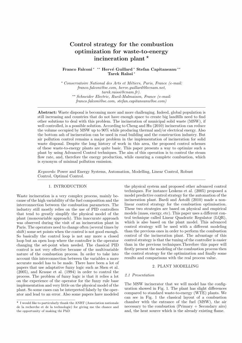
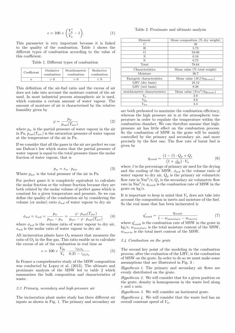
The command was tested for a typical case that is oftenencountered in incinerators. We consider a negative distur-bance of the steam flow rate and we want to see the effectof the command on our system. As it is shown in Fig. 9the disturbance rejection is done by a complementary workbetween high pressure air and primary air.

Fig. 8. Disturbance compensation of steam

Fig. 9. Air supply command, primary air in blue and highpressure air in red

The matrices values for the simulation are :

A =

−8.3333 · 10−4 00 −0.0042 00 0 −0.4179

B =

5.33 · 10−5 0 00 −4.7336 · 10−6 00 26.3468 −32.2946

C =

[1 0 00 1 00 0 0.1136

]

5. CONCLUSION

This paper propose a new way to optimize the combustionof a WTE facility by setting new optimisation criteria. In-deed the control of the waste bed height, at the beginningand at the end of the process, ensures a good combustionquality. Also in order to implement our control strategya new model of an incineration plant has been presented.Finally a multivariable control strategy has been proposedin order to cope with the insufficiency of a classical SISO(Single Input Single Output) control strategy.

REFERENCES

Bardi, S. and Astolfi, A. (2010). Modeling and control ofa waste-to-energy plant [applications of control]. IEEEControl Systems Magazine, 30(6), 27–37.

Cheng, H. and Hu, Y. (2010). Municipal solid waste (msw)as a renewable source of energy: Current and futurepractices in china. Bioresource Technology, 101(11),3816 – 3824.

Kessel, L.V., Leskens, M., and Brem, G. (2002). On-linecalorific value sensor and validation of dynamic modelsapplied to municipal solid waste combustion. ProcessSafety and Environmental Protection, 80(5), 245 – 255.

Krause, B., von Altrock, C., Limper, K., and Schafers,W. (1994). A neuro-fuzzy adaptive control strategyfor refuse incineration plants. Fuzzy Sets and Systems,63(3), 329 – 338. Industrial Applications.

Leckner, B. (1972). Spectral and total emissivity of watervapor and carbon dioxide. Combustion and Flame,19(1), 33 – 48.

Leskens, M., van Kessel, L., and Bosgra, O. (2005). Modelpredictive control as a tool for improving the process op-eration of msw combustion plants. Waste Management,25(8), 788 – 798.

Lopez, A., Roizard, D., Favre, E., and Dufour, A. (2013).Les procedes de capture du CO2. cas des unites detraitement et de valorisation thermique des dechets.Etat de l’art. RECORD, n◦11-0236/1A, 118.

Osborne, N.S. and Meyers, C.H. (1934). A formula andtables for the pressure of saturated water vapor in therange 0 to 374◦c. Research paper RP691, NationalBureau of Standards, Washington, DC, USA.

Schuler, F., Rampp, F., Martin, J., and Wolfrum, J.(1994). Taccos—a thermography-assisted combustioncontrol system for waste incinerators. Combustion andFlame, 99(2), 431 – 439. 25th Symposium (Interna-tional) on Combustion Papers.

Shen, K., Lu, J., Li, Z., and Liu, G. (2005). An adaptivefuzzy approach for the incineration temperature controlprocess. Fuel, 84(9), 1144 – 1150.